Loughborough UniversityInstitutional Repository

Experimental study of theunsteady aerodynamics the

compressor-combustorinterface of a lean burn

combustion system

This item was submitted to Loughborough University's Institutional Repositoryby the/an author.

Citation: WALKER, A.D. ...et al., 2013. Experimental study of the unsteadyaerodynamics the compressor-combustor interface of a lean burn combustionsystem. IN: 49th AIAA/ASME/SAE/ASEE Joint Propulsion Conference, SanJose, California, 14-17th July. http://dx.doi.org/10.2514/6.2013-3603

Additional Information:

• This is a conference paper.

Metadata Record: https://dspace.lboro.ac.uk/2134/19070

Version: Accepted

Publisher: Copyright c© 2013 by A. Duncan Walker , Jonathon F. Carrotte ,Graham L. Peacock , Adrian Spencer and James J. McGuirk. Published by theAmerican Institute of Aeronautics and Astronautics, Inc., with permission

Rights: This work is made available according to the conditions of the Cre-ative Commons Attribution-NonCommercial-NoDerivatives 4.0 International(CC BY-NC-ND 4.0) licence. Full details of this licence are available at:https://creativecommons.org/licenses/by-nc-nd/4.0/

Please cite the published version.

1

Experimental Study of the Unsteady Aerodynamics in the Compressor-Combustor Interface of a Lean Burn Combustion System

A. Duncan Walkeri, Jonathon F. Carrotteii, Graham L. Peacockiii, Adrian Spenceriv and James J. McGuirkv Department of Aeronautical and Automotive Engineering, Loughborough University, Loughborough,

Leicestershire, LE11 3PE, United Kingdom

Abstract To meet the technological challenges of lean burn, low emission combustion knowledge based design methodologies must be developed. This paper presents back-to-back, time-averaged and time-resolved aerodynamic measurements made using a unique state-of-the-art fully annular isothermal test facility incorporating a ½ stage axial compressor and a typical lean burn, low emission combustor geometry and either a clean or a strutted OGV/pre-diffuser system. The various measurement techniques employed (miniature five-hole probe, hot-wire anemometry, PIV) show a good level of agreement highlighting both the effect of including pre-diffuser struts and the notable unsteadiness present in the OGV/pre-diffuser system. The data presented provide the first evidence of the highly unsteady nature of the flow issuing from a pre-diffuser and potentially influencing the downstream external combustor aerodynamics.

Nomenclature

A = Area AR = Area ratio CFD = Computational Fluid Dynamics CO = Carbon monoxide CO2 = Carbon dioxide

= Static pressure coefficient h = Height L = Length LES = Large Eddy Simulations Ls = Turbulent length scale N = Rotor speed (rpm) NOx = Nitrous Oxides

= Mass flow rate M = Mach number OGV = Outlet Guide Vane P, p = Total, static pressure PIV = Particle Image Velocimetry q = Dynamic pressure r = Radius R = Gas constant T, t = Total, static temperature Tu = Turbulence Intensity

U, V, W = Velocity components in axial, radial

and circumferential direction Ublade = Rotor blade speed UHC = Unburned Hydro Carbons Va = Mid-passage axial velocity x, r, = Axial, radial and circumferential

coordinate system = Density

= Rotor flow coefficient = Total pressure loss coefficient

Superscripts: ~ = Mass weighted spatially averaged

mean value - = Area weighted spatially averaged

mean value Subscripts: 1, 2 = Arbitrary inlet, outlet stations Z = Rotor exit traverse plane A = OGV exit traverse plane B = Pre-diffuser exit traverse plane

i Lecturer in Applied Aerodynamics, e-mail: a.d.walker@lboro.ac.uk. ii Reader in Experimental Propulsion Aerodynamics, e-mail: j.f.carrotte@lboro.ac.uk. iii Research Associate, e-mail: g.l.peacock@lboro.ac.uk. iv Senior Lecturer in Thermo-fluid Dynamics, e-mail: a.spencer@lboro.ac.uk. v Professor of Aerodynamics, e-mail: j.j.mcguirk@lboro.ac.uk.

2

1.0 Introduction

Air traffic is expected to grow significantly over the next twenty years and, unless new technology is introduced, this will negatively impact the environment with increased greenhouse effects (CO2 emissions) and degradation of local air quality (NOx, particulates, CO emissions and UHC). Consequently, stringent legislation is in place and drives ambitious technological objectives agreed by the European aeronautics industry and described in ACARE’s Vision 20201. This prescribes an 80% reduction in NOx and a 50% reduction in CO2 emissions by 2020 for large civil aircraft (relative to the state-of-the-art in 2000). To meet these challenges and remain competitive in the global market the European engine industry has been addressing engine emissions in several ambitious research projects; for example INTELLECT_DMvi, IMPACT_AEvii, KIAIviii, NEWACix and LEMCOTECx.

Lean burn combustion is currently the preferred technology to meet the increasingly stringent

low NOx targets. However, the increased air flow through lean burn fuel injectors means that, in order to maintain a similar pressure drop to current rich burn designs, they are significantly larger than their rich-burn counterparts (Fig. 1). Consequently, the performance of compressor outlet guide vanes, pre-diffusers and lean burn fuel injectors are now much more closely coupled. The pre-diffuser/dump concept is currently the de facto design philosophy for the compressor-combustor interface and it is well known their performance is sensitive to both the upstream and downstream flow conditions. The effect of inlet condition and the importance of compressor exit conditions (outlet guide vane or OGV) wakes has been well characterised by, for example, Stevens et al.2, Klein3, Zierer4, Carrotte et al.5, and Barker and Carrotte6,7. Indeed diffusers in turbomachinery environments achieve a considerably higher pressure recovery than with classical “clean” ducted flow inlet conditions due to the increased turbulent mixing associated with compressor exit flow-fields. The effect of downstream flow conditions has also been characterised. For example, Walker et al.8 demonstrated that the increased air flow through the fuel injector can significantly modify the flow field within the upstream pre-diffuser, outlet guide vanes and even the last stage rotor. As the flow fraction through the injector was systematically increased from rich to lean burn levels Walker et al.8 found initially that the pre-diffuser performance deteriorated and moved close to separation. This was as a result of the reduction in the beneficial blockage effect generated by the downstream flame tube. Subsequently the overall combustor loss, which is a direct function of the pre-diffuser performance, deteriorated with Walker et al.8 measuring a 20% increase. Furthermore, at the highest injector flow rates Walker et al.8 observed that circumferential variations in the static pressure field generated by the injectors was sufficiently strong enough to significantly modify the performance of the OGV row and cause local forcing of the rotor. In order to limit this potentially damaging coupling in a further study Walker et al.9 examine the influence of dump gap at high injector flow rates. With an increase of dump gap by 50% over conventional rich burn combustion systems the forcing reduced but so did the beneficial blockage effect and as a result pre-diffuser and system performance deteriorated. As higher dump gaps, although interaction with the turbomachinery was eliminated, the pre-diffuser no longer felt any beneficial influence from the flame tube and Walker et al.9 reported evidence of flow separation.

Similarly, Barker and Carrotte10 and Ford et al.11 demonstrated that the air flow feed to fuel

injectors is strongly influenced the compressor exit conditions. Ford et al.11 numerically

vi Integrated Lean Low-Emission Combustor Design Methodology, www.intellect-dm.org vii Intelligent Design Methodologies for Low Pollutant Combustors, www.impact-ae.eu viii Knowledge for Ignition, Acoustics and Instabilities, www.kiai-project.eu ix New Aero Engine Core Concepts, www.newac.eu x Low Emissions Core-Engine Technologies, www.lemcotec.eu

3

investigated the injector feed mechanism in a lean burn system highlighting the influence of the pre-diffuser and the mismatch between the injector mean diameter and the diffuser exit height. For the centre passages of the injector, which sit directly in the compressor efflux, the feed uniformity was relatively good. However, the redistribution of flow necessary for flow to enter the injector outer passages leads to significant flow field non-uniformities. Experimental measurements downstream of an injector showed that variations attributed to the injector itself (e.g. swirl vane wakes, feed arms etc.) amounted to ±5% whereas variation generated by the upstream flow field supplying the fuel injector amounted to ±10%. These spatial non-uniformities are potentially very important as they will affect the local air-to-fuel ratio and hence the emissions performance.

In addition to increased component interaction and feed uniformity it is also important to

consider the unsteady aerodynamics of the system. It is well known, for example, that the flow field downstream of a swirl stabilised fuel injector contains unsteady features such as vortex breakdown as processing vortex cores. Several authors such as Midgely et al.12 and Dunham et al.13 have studied this experimentally and numerically but in isolation from a realistic combustor aerodynamic environment. Ford et al.11 made some limited time-resolved measurements in a representative combustor which highlighted (i) the presence of an aerodynamic instability in the injector flow field and (ii) a link in the spectral content to the upstream feed. Furthermore, it is also known that lean combustion can be fundamentally prone to thermo-acoustic instabilities (see for example Rupp et al.14). A feedback mechanism between the unsteady heat release and the system aerodynamics can potentially become self-exciting and cause damage to the combustion system. Thus, an understanding of the unsteady aspects of combustor external aerodynamics in the absence of any acoustic effects would provide important baseline information.

Ultimately, in order to realise the benefits of lean combustion and achieve low NOx and low

fuel burn (CO2) the compressor-combustor interface must be carefully managed in both a spatial and temporal sense. However, there is currently a limited amount of time-resolved experimental data available which can be used to develop understanding of the fundamental processes and subsequently establish validated knowledge based design methods. In particular, designers rely heavily on computational fluid dynamics (CFD) to understand and develop a design prior to committing to an expensive engine test programme. Unsteady CFD methodologies such are large eddy simulations (LES) are moving from the realms of academic research into mainstream design methods but they still require significant validations and are reliant on the provision of representative unsteady boundary conditions. Hence in order to address and fill this gap, the main aims of the current work were to:

To develop a fully annular isothermal test facility representative of a lean burn combustion system and use this facility to produce a database of both mean flow and unsteady flow data taken in the compressor outlet guide vane/pre-diffuser assembly.

Establish the feasibility of using Particle Image Velocimetry (PIV) in a complex fully annular test facility in order to provide planer time-resolved data which may be used to analyse coherent flow structures.

By way of illustration, the paper compares the flow in a clean pre-diffuser and one containing radial struts. In some moderns engines radial struts are often included to transfer loads or to pass various engine services (e.g. cooled-cooling air). However, they present a limiting factor in the design of the pre-diffuser. For example the interaction of the strut and end-wall boundary layers under the action of an adverse pressure gradient can generate unsteady secondary flows

4

leading to flow separation earlier than observed in un-strutted designs. Further, there is potential for the strut to be at incidence, particularly at off-design operation, exacerbating the problem. Finally, struts generate wakes incorporating unsteady vortex shedding which has been observed by Barker and Carrotte10 to influence both the flow passing down the combustor annuli and through the fuel injector. Initially a datum clean pre-diffuser was examined where the only source of unsteadiness was that issuing from the rotor and OGV. Subsequently, struts were added and their effect assessed.

The work reported herein was undertaken as part of the KIAI project (Knowledge for Ignition,

Acoustics and Instabilities). This was a four year European initiative which started in May 2009 and was financed by the European Community's Seventh Framework Programme (FP7/2007-2013) under Grant Agreement No. ACP8-GA-2009-234009FP7 .The overall aim of KIAI was to addresses innovative solutions for the development of new combustors in aero-engines. It aims at providing low NOx methodologies to be applied to design these combustors.

(a) rich

(b) lean

Figure 1: Rich and Lean Burn Combustor Architecture

5

2.0 Experimental Test Facility

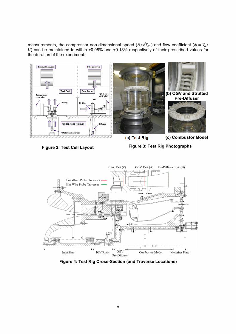
2.1 Test Cell Layout During this project all experimental data were obtained on a low speed isothermal test facility

operating at nominally atmospheric conditions. As shown in Fig. 2-4 the fully-annular test rig is mounted vertically to the test cell floor with filtered ambient air delivered to an 80 m3 under-floor plenum chamber via a large centrifugal fan. The air passes through a honeycomb flow straightener and is then accelerated over a bell-mouth intake prior to entering into the test rig. As discussed earlier, it is widely acknowledged2-6 that the inlet conditions presented to a combustor pre-diffuser have a crucial influence on its aerodynamic performance. The upstream compressor generates inlet conditions which vary both spatially and temporally and capturing the effect of these is essential to the project goals. Hence, the use of a bespoke 1½ stage axial flow compressor provides a good compromise in terms of capturing the unsteady blade wakes, secondary flows and rotor tip leakage flows that will have an important influence on downstream components whilst avoiding the costs associated with a multi-stage compressor. Downstream of the rotor are located an engine representative OGV/pre-diffuser and the combustor simulation aft of which the air exhausts into the test cell and to atmosphere via a set of louvers.

2.2 Compressor Design and Operation Design of the 1½ stage axial flow compressor (Fig. 5) was undertaken in conjunction with

Rolls-Royce plc. The philosophy in this type of test facility is to design a bespoke inlet guide vane (IGV) and rotor which will provide the correct inlet conditions (radial profiles of total pressure, pitch angles and yaw angles) to an engine representative OGV. The IGV and the rotor are not intended to directly represent engine components. However, the OGV are designed to experience nominally the same loading, in terms of DeHaller number, diffusion factor, hub/tip ratio and inlet/exit swirl angle as a typical engine OGV. Ideally, the flow in the test facility would be such that the engine non-dimensional mass flow ( √ / ) and compressor blade Reynolds number are faithfully reproduced. However, rig temperatures and pressures are so low that these operating conditions cannot be achieved. To ensure dynamic similarity with the engine aerodynamics the test rig mass flow is set sufficiently high to ensure the OGV Reynolds number, based on the chord, is greater than 1.9 x 105. According to Cumpsty15 this means that boundary layer transition occurs early enough to ensure that the OGV exit flow (unsteady wakes and secondary flows) are fully engine representative. The IGV row consists of 140 vanes which impart approximately 15º of pre-swirl onto the rotor. The rotor itself consists of 81 blades and has a tip clearance equal to 1.5% of the span. The compressor was operated at a fixed non-dimensional mass flow and non-dimensional rotor speed. At standard day conditions this amounts to a design speed of 3500 rpm ( /√ = 206.2) and flow co-efficient ( / ) of 0.379 producing a pressure ratio 1.055, a stage temperature rise of 4.9 K, an air mass flow rate of approximately 2.9 kgs-1, a mean axial velocity of 42.5 ms-1 (M = 0.125), and an OGV Reynolds number of 2.0 x 105. The flow leaves the rotor with a mean swirl angle of 45º and is returned to a nominally axial direction by the 140 OGV.

During operation of the rig the centrifugal fan, which is located in series with the test rig, is

initially used to assist in starting the compressor and then subsequently to maintain the correct operating condition (flow coefficient and mass flow rate). The operating condition of the axial flow compressor is monitored using three Furness FCO44 pressure transducers. Two of these record the inlet total, static and hence dynamic pressure giving the inlet velocity and mass flow. The third provides a reference gauge pressure at a suitable location within the test section. A single K-type thermocouple provides the inlet stagnation temperature ( ). Using these

6

measurements, the compressor non-dimensional speed ( /√ ) and flow coefficient ( /) can be maintained to within ±0.08% and ±0.18% respectively of their prescribed values for

the duration of the experiment.

(a) Test Rig

(b) OGV and Strutted

Pre-Diffuser

(c) Combustor Model

Figure 2: Test Cell Layout Figure 3: Test Rig Photographs

Figure 4: Test Rig Cross-Section (and Traverse Locations)

7

2.3 Pre-Diffuser Design Two pre-diffuser configurations were designed to sit downstream of the OGV row; one with

and one without radial struts. In line with a typical modern combustor designs geometry both pre-diffusers have a non-dimensional length (L/h1) of 3.0 and a slight outboard cant of 3.9º (see Fig. 6 and Table 1). With reference to the diffuser loading chart shown in Fig. 7 this enables an area ratio of 1.65 to be achieved for the un-strutted design. The chart illustrates the line-of- first-stall generated by Howard et al.16 and it is common design practice to back-off somewhat from this line. However, the experiments used to generate these data generally did not include compressor generated inlet conditions. As described earlier, the increased turbulent mixing and flow redistribution associated with a compressor generated flow field has been shown to reduce the likelihood of flow separation in the pre-diffuser. Consequently, the line-of-first-stall becomes a relatively good design criterion for un-strutted gas turbine combustor pre-diffusers.

As described earlier the problems associated with the addition of struts prevent area-ruling of

the strutted diffuser in order to return the area ratio to that of the clean design. Consequently the strutted diffuser utilises the same annulus lines as the clean design and, with the addition of 14 struts, has a reduced area ratio of 1.53. A corresponding line of first stall is shown in Fig. 7. The struts themselves begin at approximately 50% diffuser length, have a relatively blunt leading edge in order to tolerate any flow incidence variations and a trailing edge thickness set by the need to achieve a certain cross-sectional area (in order to meet structural requirements).

Parameter Clean Strutted Non-dimensional Length, L/h1

3.0 3.0

Area Ratio (A2/A1) 1.65 1.53 Strut Leading Edge, R/h1 - 0.09 Strut Trailing Edge, t/h1 - 0.43 Strut Blockage - 7.3% Strut Fillet Radius, r/h1 - 0.16

Table 1: Pre-Diffuser Geometry

2.4 Lean Burn Combustor Simulation The test rig was designed to include a combustor simulation representative of a modern lean

burn configuration (Fig. 3, 4 and 8) and the simulation is wholly representative up to the point at which the flow enters the combustor annuli. The fuel injectors and the cowl consist of rapid prototype models which include all the main air-washed surfaces such as the swirl vanes etc. However, to simplify the downstream geometry and limit overall costs no attempt was made to model small scale features, such as cooling flows, which have limited influence on the external aerodynamics. Similarly, the combustor annuli and the flame tube are modelled by a solid surface omitting all flow features (dilution holes, cooling tile flows etc.). The mass flow distribution through the combustor simulation was set at the aft end of the test rig using suitably sized and metered orifice holes such that 50% of the compressor efflux passed through the injector models with the remaining split equally between the inner and outer annuli. Ultimately the combustor simulation is more than sufficient to ensure that any downstream/upstream component interaction caused by the proximity of the cowl or the circumferential variation in cowl/injector flow will be captured in the experiment.

8

Figure 5: Schematic of IGV, Rotor and OGV

Figure 6: Pre-Diffuser Geometry

Figure 7: Diffuser Loading Chart Figure 8: Solid Model of Test Rig

2.5 Instrumentation and Data Acquisition The test rig utilised a bespoke control system which can be integrated with various data

acquisition techniques to monitor/adjust the compressor operating point, perform probe traversing and acquire experimental data. The test rig instrumentation relies upon a PC running LabView in communication with a 16-bit National Instruments data acquisition system. The latter provides analogue to digital conversion of up to 16 channels of time-averaged voltage information, together with the conditioning and recording of up to five K-type thermocouple signals. In addition, up to four RS232 serial links enable the PC to communicate with a DC servo probe traverse system, two motor controllers and a digital barometer. The two motor controllers provide full control of the DC motors used to drive both the centrifugal fan and the rotor of the 1½ stage compressor. Furness FCO44 differential pressure transducers are used both to monitor the operating conditions and to record information from pneumatic probes. The LabView software developed to integrate the PC and the instrumentation system employs an

9

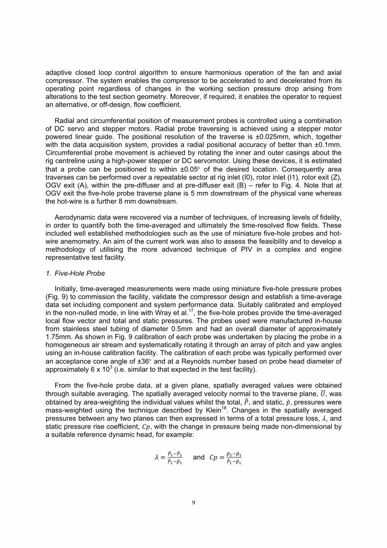
adaptive closed loop control algorithm to ensure harmonious operation of the fan and axial compressor. The system enables the compressor to be accelerated to and decelerated from its operating point regardless of changes in the working section pressure drop arising from alterations to the test section geometry. Moreover, if required, it enables the operator to request an alternative, or off-design, flow coefficient.

Radial and circumferential position of measurement probes is controlled using a combination

of DC servo and stepper motors. Radial probe traversing is achieved using a stepper motor powered linear guide. The positional resolution of the traverse is ±0.025mm, which, together with the data acquisition system, provides a radial positional accuracy of better than ±0.1mm. Circumferential probe movement is achieved by rotating the inner and outer casings about the rig centreline using a high-power stepper or DC servomotor. Using these devices, it is estimated that a probe can be positioned to within ±0.05 of the desired location. Consequently area traverses can be performed over a repeatable sector at rig inlet (I0), rotor inlet (I1), rotor exit (Z), OGV exit (A), within the pre-diffuser and at pre-diffuser exit (B) – refer to Fig. 4. Note that at OGV exit the five-hole probe traverse plane is 5 mm downstream of the physical vane whereas the hot-wire is a further 8 mm downstream.

Aerodynamic data were recovered via a number of techniques, of increasing levels of fidelity,

in order to quantify both the time-averaged and ultimately the time-resolved flow fields. These included well established methodologies such as the use of miniature five-hole probes and hot-wire anemometry. An aim of the current work was also to assess the feasibility and to develop a methodology of utilising the more advanced technique of PIV in a complex and engine representative test facility.

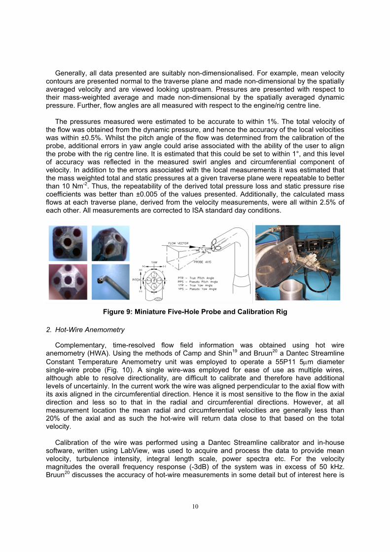
1. Five-Hole Probe

Initially, time-averaged measurements were made using miniature five-hole pressure probes

(Fig. 9) to commission the facility, validate the compressor design and establish a time-average data set including component and system performance data. Suitably calibrated and employed in the non-nulled mode, in line with Wray et al.17, the five-hole probes provide the time-averaged local flow vector and total and static pressures. The probes used were manufactured in-house from stainless steel tubing of diameter 0.5mm and had an overall diameter of approximately 1.75mm. As shown in Fig. 9 calibration of each probe was undertaken by placing the probe in a homogeneous air stream and systematically rotating it through an array of pitch and yaw angles using an in-house calibration facility. The calibration of each probe was typically performed over an acceptance cone angle of ±36 and at a Reynolds number based on probe head diameter of approximately 6 x 103 (i.e. similar to that expected in the test facility).

From the five-hole probe data, at a given plane, spatially averaged values were obtained

through suitable averaging. The spatially averaged velocity normal to the traverse plane, , was obtained by area-weighting the individual values whilst the total, , and static, ̌, pressures were mass-weighted using the technique described by Klein18. Changes in the spatially averaged pressures between any two planes can then expressed in terms of a total pressure loss, , and static pressure rise coefficient, , with the change in pressure being made non-dimensional by a suitable reference dynamic head, for example:

and

10

Generally, all data presented are suitably non-dimensionalised. For example, mean velocity contours are presented normal to the traverse plane and made non-dimensional by the spatially averaged velocity and are viewed looking upstream. Pressures are presented with respect to their mass-weighted average and made non-dimensional by the spatially averaged dynamic pressure. Further, flow angles are all measured with respect to the engine/rig centre line.

The pressures measured were estimated to be accurate to within 1%. The total velocity of

the flow was obtained from the dynamic pressure, and hence the accuracy of the local velocities was within ±0.5%. Whilst the pitch angle of the flow was determined from the calibration of the probe, additional errors in yaw angle could arise associated with the ability of the user to align the probe with the rig centre line. It is estimated that this could be set to within 1°, and this level of accuracy was reflected in the measured swirl angles and circumferential component of velocity. In addition to the errors associated with the local measurements it was estimated that the mass weighted total and static pressures at a given traverse plane were repeatable to better than 10 Nm-2. Thus, the repeatability of the derived total pressure loss and static pressure rise coefficients was better than ±0.005 of the values presented. Additionally, the calculated mass flows at each traverse plane, derived from the velocity measurements, were all within 2.5% of each other. All measurements are corrected to ISA standard day conditions.

Figure 9: Miniature Five-Hole Probe and Calibration Rig

2. Hot-Wire Anemometry

Complementary, time-resolved flow field information was obtained using hot wire

anemometry (HWA). Using the methods of Camp and Shin19 and Bruun20 a Dantec Streamline Constant Temperature Anemometry unit was employed to operate a 55P11 5m diameter single-wire probe (Fig. 10). A single wire-was employed for ease of use as multiple wires, although able to resolve directionality, are difficult to calibrate and therefore have additional levels of uncertainly. In the current work the wire was aligned perpendicular to the axial flow with its axis aligned in the circumferential direction. Hence it is most sensitive to the flow in the axial direction and less so to that in the radial and circumferential directions. However, at all measurement location the mean radial and circumferential velocities are generally less than 20% of the axial and as such the hot-wire will return data close to that based on the total velocity.

Calibration of the wire was performed using a Dantec Streamline calibrator and in-house

software, written using LabView, was used to acquire and process the data to provide mean velocity, turbulence intensity, integral length scale, power spectra etc. For the velocity magnitudes the overall frequency response (-3dB) of the system was in excess of 50 kHz. Bruun20 discusses the accuracy of hot-wire measurements in some detail but of interest here is

11

the accuracy of the techniques as the flow becomes increasingly unsteady and approaches separation. For turbulence intensities approaching 30% the errors are generally less than 4%. However, a single hot wire cannot resolve any flow reversal which may occur at higher turbulence intensities. This is referred to as a rectification error and begins at intensities in excess of 35% although the frequency of rectification is less than 2% up to intensities of 50%.

Figure 10: 5m Diameter Hot-Wire and DAQ Software

3. Particle Image Velocimetry (PIV)

One of the main aims of this piece of work was to develop a methodology to enable PIV

measurements to be made in existing complex fully annular test facility. The advantages of PIV are that, to a large degree, it is a non-intrusive technique which can provide instantaneous measurement of velocity over an entire two-dimensional plane (or field of view). In addition to providing traditional data such as mean velocity, turbulence intensity, integral length scale, power spectra etc., the planar nature of PIV allows for the potential of the unsteady flow field to be analysed in much more detail. For example, with advanced PIV it is possible to extract information on coherent structures which may exist in the unsteady flow field. However, the challenges of successfully employing PIV on such a complex test facility should not be underestimated. These include:

suitable seeding of the flow, delivery of the laser light sheet correctly and accurately positioned with the light intensity

and thickness of the sheet optimised for the experiment, a camera (or cameras) properly orientated and the focal parameters optimised to ensure

the best quality image, and optimisation of the timing synchronisation and inter-frame settings. The specifics of how these issues were addressed will be presented later in the paper

(Section 4.0). However, for more detail on the fundamentals of the technique to reader is referred to Raffel et al.21.

12

3.0 Results and Discussion: Five-Hole Probe and Hot-Wire Measurements

As part of commissioning a check was made to ensure that there was no notable

circumferential variation in the flow entering the test rig and passing through the rotor and OGV. This was achieved by circumferentially traversing wall static tappings positioned on the outer casing at rotor and OGV exit as shown in Fig. 11. No notable circumferential variation was observed at rotor exit; the small saw-tooth variations amount to less than 2% of the rotor exit dynamic pressure and are due to the upstream potential field from the OGV. However at OGV exit there are variations in both the clean and strutted case. For the clean diffuser a slight variation (5% of dynamic) can be seen in line with the location of the fuel injectors. This circumferential variation is generated by the localised high mass flow rates of the lean burn injectors. However, the magnitude of this variation at OGV exit is little more than the local variation caused by the OGV. For strutted pre-diffuser there is a much larger circumferential variation caused by the introduction of the struts. An increase of the local static pressure in line with the struts of order 15% of the OGV exit dynamic is seen. These results are significant and suggest that the rotor itself does not feel any influence from the pre-diffuser struts or the fuel injectors but the OGV certainly do. The latter will be examined further in Section 3.2.

(a) Rotor Exit (b) OGV Exit

Figure 11: Influence of Struts - Circumferential Variation of Wall Static Pressure at Rotor and OGV Exit

3.1 Rotor Exit (Z) Figure 12 plots circumferentially averaged profiles constructed from five-hole probe area

traverses at rotor exit. These were performed over a repeatable OGV sector (~2.57°) for both the clean and strutted pre-diffusers, in line and between the struts. The profiles confirm that the introduction of struts has negligible effect on the flow at rotor exit. Indeed, for the profiles shown the data are identical within experimental accuracy. In general the rotor produces a hub-bias flow with a reduced velocity on the outer wall and it is usual for the outer casing boundary layer to be larger due to rotor tip leakage flows. This can be seen in the total pressure profile which shows a notable reduction in performance over the last 20% of the passage. As will be seen later, this has a fundamental impact on the performance of the OGV and, in particular, the pre-diffuser. The rotor is designed to give an average of approximately 45 of swirl and the profile indicates that over the mid-passage this is achieved. However, as expected in regions of lower axial velocity near the casings this increases the local flow angle and towards the outer casing the flow angle increases above 60. Contours from the five-hole probe measurements are presented in Fig. 13. The rotor exit measurements were not phase locked, data were not captured with the rotor blade (and wake) in the same spatial location and the time-averaged

13

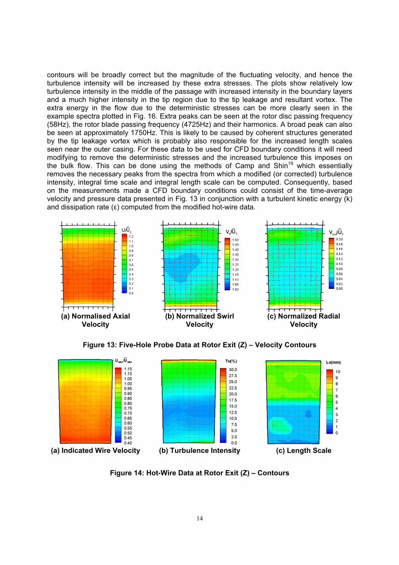
period was equated to nearly 20,000 blade passing incidents. Consequently, the contour plots give an averaged view of the flow field including any bulk effect of the rotor blade wake but do not show directly the rotor wake itself. The contours still show some amount of circumferential non-uniformity due to the propagation of the wake from the IGV and the upstream potential field of the OGV; these are most evident in the contours of axial velocity.

(a) Normalised Axial Velocity

(b Yaw (Swirl) Angle

(c) Normalised Total Pressure

(d) Normalised Static Pressure

Figure 12: Five-Hole Probe Data at Rotor Exit (Z) - Circumferentially Averaged Profiles

The corresponding hot-wire data are presented in Fig. 14. The contours of velocity exhibit

some differences to the axial velocity contours due to the fact that the single wire is also partly influenced by the circumferential and radial velocity components. Additionally, the fluctuating velocity and length scales plotted in Fig. 15 are not a true reflection of the turbulence at rotor exit as the measurements were not phase locked. Hence the turbulent data include the extra deterministic stresses induced by the periodic passing of the rotor wake. The shape of the

14

contours will be broadly correct but the magnitude of the fluctuating velocity, and hence the turbulence intensity will be increased by these extra stresses. The plots show relatively low turbulence intensity in the middle of the passage with increased intensity in the boundary layers and a much higher intensity in the tip region due to the tip leakage and resultant vortex. The extra energy in the flow due to the deterministic stresses can be more clearly seen in the example spectra plotted in Fig. 16. Extra peaks can be seen at the rotor disc passing frequency (58Hz), the rotor blade passing frequency (4725Hz) and their harmonics. A broad peak can also be seen at approximately 1750Hz. This is likely to be caused by coherent structures generated by the tip leakage vortex which is probably also responsible for the increased length scales seen near the outer casing. For these data to be used for CFD boundary conditions it will need modifying to remove the deterministic stresses and the increased turbulence this imposes on the bulk flow. This can be done using the methods of Camp and Shin19 which essentially removes the necessary peaks from the spectra from which a modified (or corrected) turbulence intensity, integral time scale and integral length scale can be computed. Consequently, based on the measurements made a CFD boundary conditions could consist of the time-average velocity and pressure data presented in Fig. 13 in conjunction with a turbulent kinetic energy (k) and dissipation rate (ε) computed from the modified hot-wire data.

(a) Normalised Axial

Velocity (b) Normalized Swirl

Velocity (c) Normalized Radial

Velocity

Figure 13: Five-Hole Probe Data at Rotor Exit (Z) – Velocity Contours

(a) Indicated Wire Velocity (b) Turbulence Intensity (c) Length Scale

Figure 14: Hot-Wire Data at Rotor Exit (Z) – Contours

15

Figure 15: Sample Hot-Wire Spectra at Rotor Exit (Z)

3.2 OGV Exit (A) To quantify any upstream effect of the struts at OGV exit five-hole probe area traverses were

made both in line with and between the fuel injectors, and therefore, both between and in line with the pre-diffuser struts respectively (note that the struts are located mid-way between injectors – refer to Fig. 16). Mass-weighted performance data computed from these traverses confirm that the overall performance of the OGV is indeed slightly modified by the presence of the fuel injectors and pre-diffuser struts (Table 2). Locally, in line with the injectors the pre-diffuser efflux accelerates whereas between it stagnates on the flame tube head. This sets up a circumferential variation in static pressure, which although small at OGV exit, is sufficient to marginally alter the OGV performance. With the struts fitted the OGV performance between the struts does not alter and the OGV (and the pre-diffuser) are effectively ignorant to the presence of the struts. However, in line with the struts the OGV performance is slightly increased; the blockage generated by the struts is beneficial to the diffusion process through the OGV row giving rise to an increased static pressure recovery. However, the effect of the injector and the struts at OGV exit is not clearly evident in the flow field in either the circumferentially averaged profiles (Fig. 17) or the contour plots (Fig. 18). Indeed within experimental error there is no difference in the measured non-dimensional velocity or flow angle and only a small variation in the total pressure in line with or between injectors and/or struts. In fact it is only in the static pressure where a slight measurable difference is seen.

Clean Diffuser 0.144 / 0.129 0.466 / 0.477 Strutted Diffuser

0.139 / 0.124 0.450 / 0.490

Table 2: OGV Performance Data (in line / between injectors)

Figure 16: OGV Exit Traverse Locations

At OGV exit the velocity the velocity profile seems less hub bias than at rotor exit but the total

pressure profile still shows a large deficit in the outer portion of the passage. Similarly the yaw angle, which is designed to be nominally zero, increases significantly toward the outer wall. The velocity contours show the clearly defined OGV wakes and illustrate that the wake noticeably

16

increases in thickness towards the outer casing. This is due to a combination of the inboard bias at rotor exit, a high outboard incidence onto the OGV, rotor tip vortices and the secondary flows developing within the OGV. The flow vectors in Fig. 18 represent the radial and circumferential velocity components and show the rotational nature of the secondary flows. This type of flow has been intensely studied (see for example Langston22, Sieverding and Van den Bosche23 and Sharma and Butler24) and is generated as the approaching boundary layer rolls up to produce horse-shoe vortices which then combine to form a passage vortex (often referred to as loss cores). Although these flows are a source of extra loss they are also beneficial to the diffuser flow. They promote turbulent mixing and encourage movement of higher momentum core flow into the end-wall boundary layers thus enabling them to tolerate higher levels of diffusion.

In summary, the five-hole probe data suggest that the flow entering the pre-diffuser is not ideal. The profile is inboard biased, the outer wall boundary layer relatively thick, there is high localised swirl near the outer wall and the OGV loss cores are relatively large. Given that the pre-diffuser is also outboard canted and the aerodynamic loading highest on the outer wall these feature can potentially combine to contribute to the earlier onset of flow separation.

The corresponding hot-wire data are plotted in Fig. 19-21. The non-dimensional velocity agrees well with the five-hole probe data. The flow is almost axial at OGV exit so the velocity indicated by the hot-wire should be close to the axial velocity measured by five-hole probe. The fluctuating velocity highlights the high shear either side of the wake which promotes the rapid circumferential mixing of the wake. The data also reveal two regions of high turbulence intensity. Firstly, as expected the outer region exhibits high turbulence levels due to the rotor tip vortices. However, secondly, in the mid-passage the turbulence intensity is also significantly high at 25-30%. For levels above 35% rectification of the hot-wire signal occurs as a single hot-wire cannot resolve flow direction. Thus, although the time-averaged velocity of the flow in this region is relatively high, the turbulence intensity suggests that some upstream transient separation may exist. This observation was supported by examination of the CFD used to design the OGV which revealed (Fig. 22) a region of flow reversal on the OGV at the corresponding location. Although it is not uncommon to have small region of flow separation on compressor OGV it is undesirable as far as the diffuser is concerned. It contributes to the larger measured wakes and loss cores, increases the total pressure loss, introduces an aerodynamic blockage which may cause an undesirable redistribution of the flow, and ultimately can promote earlier separation.

Some example spectra are presented in Fig. 23. Small peaks are still seen corresponding to the rotor disc and blade passing frequencies but these are much reduced in energy content from rotor exit. There is no longer any evidence of a peak corresponding to the rotor tip vortex and the only point which reveals any energy containing structure is point 160 which shows a weak broad band at approximately 700Hz probably produced by the OGV separation.

17

(a) Normalised Axial Velocity

(b) Yaw (Swirl) Angle

(c) Normalised Total Pressure

(d) Normalised Static Pressure

Figure 17: Five-Hole Probe Data at OGV Exit (A) - Circumferentially Averaged Profiles

18

Clean Diffuser Strutted Diffuser

(a) Between Injectors (b) In line Injectorsr

(c) Between Injectors

(d) In line Injectors

Figure 18: Five-Hole Probe Data at OGV Exit (A) - Velocity Contours and Secondary Flow Vectors

Clean Diffuser Strutted Diffuser

(a) Between Injectors (b) In line Injectorsr

(c) Between Injectors

(d) In line Injectors

Figure 19: Hot-Wire Data at OGV Exit (A) – Velocity Contours

Clean Diffuser Strutted Diffuser

(a) Between Injectors (b) In line Injectorsr

(c) Between Injectors

(d) In line Injectors

Figure 20: Hot-Wire Data at OGV Exit (A) – Turbulence Intensity

19

Clean Diffuser Strutted Diffuser

(a) Between Injectors (b) In line Injectorsr

(c) Between Injectors

(d) In line Injectors

Figure 21: Hot-Wire Data at OGV Exit (A) – Length Scales

Figure 22: Design CFD – showing iso-surface of U = 0 ms-1

Figure 23 Hot-Wire Data at OGV Exit (A) - Selected Spectra

20

3.3 Pre-Diffuser Exit (B)

At diffuser exit five-hole probe area traverses were made over a complete sector (strut-to-strut) but to maintain the measurement resolution this had to be broken down into ten separate sectors each equivalent to one OGV space (Fig. 24). Axial velocity, total and static pressure contours are plotted over the full sector for both the clean and the strutted diffuser in Fig. 25-27. The contours show that the OGV wakes are still evident, particularly in the inboard section. Outboard, the wakes are less evident and there is a much greater flow deficit leading to a strongly inboard bias in the profile. Around the outer wall there are small regions of low velocity (less than 20% of the mean). This suggests that the flow in these regions may be exhibiting some transient separation. Comparing the clean and strutted diffusers shows that there is no noticeable difference in the flow field between the struts. The diffuser flow only seems to “feel” the presence of the struts in the immediately adjacent sectors. Here the merging of the strut wall and diffuser end wall boundary layers results, not unexpectedly, in a corner stall. This appears slightly worse on the right hand side of the plot and is a result of the strut being slightly at incidence; the OGV exit swirl angle is not quite zero. The time-averaged data suggest that the corner stall is not particularly large but as this is an unsteady phenomenon it will potentially grow and propagate either periodically or indeed randomly. Of interest would be what time-resolved effect this would have in the downstream combustor.

The mean velocity contours from the hot-wire data (Fig. 28) show a good general agreement

with the five-hole probe data although they suggest that the flow closer to the outer wall has a lower velocity and therefore closer to separation. Indeed in these regions the measured turbulence intensity (Fig. 29) suggests a high level of fluctuation. However, in these regions the accuracy of the single hot-wire technique comes into question. As mentioned before a single wire is insensitive to the direction of the fluctuating velocity and at high turbulence intensities rectification of the signal can occur. At turbulence intensities above 35% this begins to increase the absolute error in the hot-wire data. Figure 29 shows intensities well in excess of 50% near the tip region and adjacent to the strut. Although, this means that the absolute values of mean and RMS velocity are perhaps unreliable it confirms that the flow in these regions contains a high degree of unsteady behaviour. However, selected spectra from the hot-wire measurements (Fig. 30) show that the disc frequency can still be observed but there are no broad peaks and hence no indication of any coherent structures.

21

Figure 24: Pre-Diffuser Exit Traverse Locations

(a) Clean Diffuser (b) Strutted Diffuser

Figure 25: Five-Hole Probe Data at Pre-Diffuser Exit (B) - Velocity Contours

(a) Clean Diffuser (b) Strutted Diffuser

Figure 26: Five-Hole Probe Data at Pre-Diffuser Exit (B) – Total Pressure Contours

(a) Clean Diffuser (b) Strutted Diffuser

Figure 27: Five-Hole Probe Data at Pre-Diffuser Exit (B) – Total Pressure Contours

22

Between Injectors In line with Injectors Between Injectors In line with Injectors

(a) Clean Diffuser (b) Strutted Diffuser

Figure 28: Hot-Wire Data at Pre-Diffuser Exit (B) – Velocity Contours

Between Injectors In line with Injectors Between Injectors In line with Injectors

(a) Clean Diffuser (b) Strutted Diffuser

Figure 29: Hot-Wire Data at Pre-Diffuser Exit (B) – Turbulence Intensity

Figure 30: Hot-Wire Data at Pre-Diffuser Exit (B) - Selected Spectra

23

4.0 Results and Discussion: PIV Measurements

4.1 Preliminary Measurements One of the main challenges of introducing PIV into an existing complex fully annular test

facility was obtaining suitable optical access for both laser light sheet and camera. Thus, for initial development of the measurement strategy, attention was focussed on the flow at OGV exit but with the pre-diffuser removed. In this simplified the light sheet was delivered directly through the Perspex outer casing of the rig with viewing of the illuminated area via a camera endoscope with a 90° side port adapter (this is referred to as an ‘r-θ plane’ measurement). The complexities of rotor flow and OGV interaction were thus fully included, but optical access was as simple as possible. To ensure that removal of the pre-diffuser did not alter the OGV efflux a series of 5-hole probe measurements were made in this simplified configuration. Figure 31 illustrates the resultant measurements showing only very small differences with and without the pre-diffuser. Hence the proposed simplification was a valid set-up to begin development of the best optical arrangements for PIV measurement.

With Diffuser Without Diffuser With Diffuser Without Diffuser (a) Axial Velocity (b) Total Pressure

Figure 31: Five-Hole Probe Data at Pre-Diffuser Exit (B)

4.2 PIV Set-up Details

Seeding

For PIV measurements it is vital that appropriate tracer particles are used that accurately follow the flow and scatter sufficient light for accurate recording. Atomised Shell Ondina oil, a low-viscosity oil with particles of maximum 2μm diameter, was selected based on previous airflow PIV measurements at Loughborough. The oil particles have a density somewhat greater than air, but have been shown by Hollis25 to be suitable for airflow applications, having a particle velocity lag of only Us = 0.294 ms-1 and a low particle response time of τp = 9.8 μs. The oil-based nature of the seeding presents issues related to condensation and dispersal to atmosphere; alcohol-based seeding was considered, however this was dismissed due to health and safety concerns. The oil seeding was produced and distributed to the flow using a TSI six-jet atomiser. This was positioned upstream of the rig, at inlet to the bell-mouth, and it was found that seeding could easily be tracked through the rotor (with only small circumferential deviation)

24

to measurement location. Thus seeding was supplied such the same OGV sector was used in the PIV measurements as for the five-hole probe. Care was taken to adjust the level of seeding to ensure there were three or more particle pairs per interrogation window, in order to increase signal to noise ratio, but also to use the minimum number of jets to achieve this in order to prevent condensation of the seed oil on rig surfaces.

Light Sheet Generation

For illumination of seed particles a laser light sheet was generated using a Litron Nano L120-20 Nd: YAG laser. The light sheet was directed at the plane of interest using a light arm with a cylindrical (50 mm) lens to produce a sheet of approximately 1 mm thickness. Throughout the course of testing the biggest challenge to successful measurements was achieving sufficient illumination of the particles for optimum capture by the camera. This issue was exacerbated by the use of the endoscope attachment described later. The camera and light sheet arrangement was such that particles could be tracked in the majority of locations; however several factors contributed to reduced seeding visibility in particular regions of the field of view (FoV). The primary factor contributing to this was reflection from rig surfaces, most significantly the OGV ring and pre-diffuser ring, resulting in glare and scattered light. Condensation of seeding oil mist on these same components and the inner wall of the annular outer casing was also found to increase the effect of reflection, and led to further light scattering through increased diffraction of the light sheet by the thick casing. Reflections from the specified components caused seeding particles in particular areas of the FoV to be obscured, in some cases making measurement impossible. This was particularly pronounced at OGV exit, since the OGV ring was manufactured from opaque white material as opposed to the clear Perspex pre-diffuser ring. Continued deposition of seeding particles led to an increase in reflection with time.

Diffraction of the light sheet through the thick outer casing resulted in an expansion of the

beam, also marginally reducing the power of the sheet. This effect was initially minor, but was observed to increase significantly due to condensation of oil mist on the inside wall of the casing at the point where the beam enters the rig. Seeding deposition on the outer casing produced localised dropout of vectors not restricted to the vicinity of the structural components visible within the FoV. An alternative technique that would eliminate the problem of light sheet diffraction through the casing would be to employ a laser endoscope. This was considered but not followed up since additional mechanical alterations to the rig would be required. For future experiments, benefits may be achieved by blowing a film of air over the inside wall of the outer casing to prevent condensation, this should significantly reduce the impact without affecting the flow field emerging from the OGV.

Camera Details

Figure 32 illustrates three configurations used to observe the flow in an x-r plane and an r- plane at OGV exit and pre-diffuser exit. In order to view these planes deep within the test rig it was necessary to use an endoscope with a 90° side port adapter. Images were then captured using an Imager Intense 1-Megapixel camera with a 60mm lens. The 60mm lens was preferred over 50mm and 120mm lenses based upon a compromise between FoV and aperture size, influencing the light intensity. The FoV for the 50mm lens was too wide, giving insufficient resolution, whereas the aperture for the 120mm lens did not allow sufficient light into the camera. The use of an endoscope impacts negatively upon the image clarity that can be achieved due to a reduced orifice size and the associated significant reduction in image light intensity. Despite this, illumination levels remained sufficient for particle motion to be tracked adequately for successful PIV measurements. Additionally, images captured through an endoscope demonstrate a greater degree of radial distortion, although use of a calibration plate allowed the impact of the distorted ‘fish-eye’ effect to be removed. In addition to reduced light

25

intensity, positioning the endoscope within the rig between the OGV or pre-diffuser and the combustor placed it directly in the path of the seeding particles. Not surprisingly this was found to result in the oil mist condensing on the endoscope and eventually obscuring the view. To negate this effect a purge device was used to pass compressed air over the endoscope mirror and prevent oil from condensing on the end of the periscope attachment.

(a) OGV Exit r-� (b) OGV Exit x-r (c) Pre-Diffuser Exit x-r

Figure 32: Laser Optics and Camera/Endoscope Set-Up

4.3 Experimental Procedure

Measurement Planes Both an r-θ plane and an x-r plane were used at OGV exit, whilst only x-r plane data were

taken at pre-diffuser exit (Fig. 32). Secondary (radial and circumferential) velocity components were captured by arranging the camera endoscope and light sheet to view an r-θ plane whereas the x-r plane gave axial and radial velocity components. However, the ability to rotate the rig circumferentially meant that r-θ plane data were also captured at various circumferential locations by traversing the rig circumferentially over a single OGV passage azimuthal sector (~2.57º) with measurements taken on 11 uniformly spaced x-r planes to enable a complete r-θ map of either axial or radial velocity to be constructed.

Data capture

Image pairs were captured at a frequency of 3Hz (individual frames should be statistically independent of each other) with an inter-frame time of ∆t = 2 μs for measurements in the r-θ plane and ∆t = 6-10 μs in the x-r plane. This variation was due to the large difference in the through-plane velocity for the two planes. The range of times for the x-r measurements was due to the varying circumferential velocity for planes between and in-line with the OGVs. Example instantaneous vectors and processed time-mean axial velocity contours for single x-r plane measurements at OGV and pre-diffuser exit are illustrated in Fig. 33. Typically 750 instantaneous image pairs were captured for each measurement plane from which time-averaged mean and RMS fluctuating velocities were determined. Vector time-averaging was based on at least 500 frames for 85% of locations in the FoV; typically 95% of these were first choice vectors. However, the combined effect of condensation and reflections resulted in local regions in which significantly fewer vectors were returned. This is illustrated by the white regions in Fig. 33(b). In total at pre-diffuser exit 8% of measurement locations returned less than 50% of

26

the possible instantaneous vectors, and a small number (4%) returned fewer than 25% validated vectors. At most points a sufficiently large sample size was available, but at a few points the small sample size produced spurious turbulence RMS values and these points have been omitted in the plotted data. Due to the larger reflection problem at OGV exit more data dropout occurred with (in the worst case) only 33% of locations returning validated vectors in more than 500 frames. This level of dropout was largely restricted to locations less than 8 mm downstream of the pneumatic probe OGV exit measurement plane. For x > 8 mm 85% of measurement locations returned vectors in more than 500 frames. For this for this reason the OGV exit r-θ plane for the PIV measurements was positioned at x = 8 mm (as indicated by the dashed line in Fig. 33). This analysis means that axial and radial velocity statistical data could not be accurately extracted from the PIV data precisely at x = 0 mm (i.e. corresponding to the five-hole probe data at OGV exit), which makes direct comparison between pneumatic probe and PIV data problematic as will be discussed below. However, due to the reduced reflection problem at pre-diffuser exit, axial and radial velocity data can be directly compared at the exit (B) between five-hole probe, hot-wire and PIV data.

(a) Instantaneous Vectors (b) Mean Axial Velocity Contours

Figure 33: PIV Data on Single x-r Plane

4.4 Mean Velocity Data

OGV Exit (A)

PIV measurements of axial velocity, non-dimensionalised using the area-weighted average velocity in the OGV exit plane, are presented in Fig. 34. The PIV data potted were extracted from a compilation of x-r plane information at the closest distance downstream where valid data over the whole sector were available. It can be seen that the distribution obtained using PIV is very similar compared to previous five-hole probe and hot-wire data. Some of the difference can be explained because, for reasons discussed above, a measurement comparison at precisely the same axial plane is not possible. In fact the hot-wire data, due to probe geometry, were taken at slightly different axial locations. In terms of velocity magnitude, the difference in axial position, and the extra mixing out of the OGV wake that has occurred, results in the maximum velocity for PIV measurements being approximately 10% lower. The hot-wire and PIV are closer (because of the smaller axial shift), indicating a wider OGV wake towards the outer wall. Note also there is a small shift circumferentially of the OGV wake between data sets, possibly caused by extra circumferential movement as result of the small residual swirl left by the OGV.

A similar comparison of time-averaged radial velocity contours is presented in Fig. 35 and

compared to the five-hole probe data. Similar regions of high and low velocity, and in broadly similar locations, may be identified in both measurements (although note the maximum value of the radial velocity is only ~12% of the mean axial velocity). Variation in the peak positive

27

magnitude is apparent, but again the axial shift of 10 mm between the measurement planes must be considered. As a cross-check on the PIV data, the radial velocity contours shown in Fig. 35(b) were extracted from PIV measurements conducted directly with an the r-θ plane FoV and in Fig. 35(c) they were compiled from a series of measurement planes in x-r plane. Whilst there is some degree of deviation between the two the agreement is encouraging – given there will likely be quite different measurement errors for the two PIV data sets. There is little doubt that differences are primarily a function of the single camera arrangement and it is considered that the quality of secondary velocity measurements could be improved significantly through the use of stereo-PIV.

(a) Five-Hole

Probe Data (x = 0 mm)

(b) Hot-Wire Probe Data (x = 8 mm)

(c) PIV Data (x = 10 mm), r-��Plane Constructed from x-r

Plane Data

Figure 34: Comparison of Axial Velocity Contours at OGV Exit

(a) Five-Hole Probe Data

(x = 0 mm) (b) PIV Data (x = 10 mm) r-��Plane Measurement

(c) PIV Data (x = 10 mm) r-��Plane Constructed

from x-r Plane Measurements

Figure 35: Comparison of Radial Velocity Contours at OGV Exit

Pre-Diffuser Exit (B)

A comparison of normalised axial velocity contours measured at pre-diffuser exit using PIV, a five-hole probe and a hot-wire is presented in Fig. 36. Again the agreement is good; a small

28

region is visible in the bottom right of the PIV image where data quality was in sufficient, but apart from this the contour maps are close. In this case no significant axial shift is present between various measurement planes. In all three images there is clear evidence that all the low momentum fluid has accumulated near the outer wall of the pre-diffuser, and this is obviously the critical region for flow separation. On the evidence of these images it is highly unlikely that the area ratio of the pre-diffuser could have been further increased without separation occurring.

A comparison of mean radial velocity presented in Fig. 37 and again the agreement is good,

with only minor deviations apparent around small regions where the PIV data is poor. Unlike at the OGV exit plane, this time there is no discrepancy in peak magnitudes between five-hole probe and PIV data.

(a) Five-Hole Probe (b) Hot-Wire Probe (c) PIV Data

Figure 36: Comparison of Axial Velocity Contours at Pre-Diffuser Exit

(a) Five-Hole Probe Data (b) PIV Data

Figure 37: Comparison of Radial Velocity Contours at Pre-Diffuser Exit

29

4.5 . Turbulence Statistics Given the disparity in axial location problem at OGV exit explained earlier, although

turbulence data was available from PIV measurements, it was decided that for data quality reasons attention should be focussed on pre-diffuser exit only.

Pre-Diffuser Exit (B)

Figure 38 presents a comparison of turbulence intensity between hot-wire and PIV data at pre-diffuser exit. The PIV data represent an evaluation based on axial component only, whereas the single hot-wire wire used will respond mainly to the velocity component normal to the wire. This comparison is believed reasonable as the axial component dominates the flow as indicated the above discussion. The contours of turbulence intensity broadly show good agreement. Again, due to reflection problems, the PIV data show signs of noise and low data quality near the inner wall. However, in terms of the unsteady flow characteristics, it is the outer wall which is of most interest. Here the peak turbulence intensities are very high (> 50%). As previously discussed this calls into question the validity of the hot-wire data due to linearization and rectification errors. The PIV data were extracted from an x-r plane where there was no high through-flow component and therefore the PIV data quality was high. Since PIV involves no linearization approximation and can resolve change in sign of the in-plane components, the high levels captured by the PIV are likely to be accurate. Thus, despite the mean velocity data from all techniques showing a time-averaged positive velocity, this suggests the occurrence of intermittent separation is highly likely. Indeed this is confirmed in Fig. 39 which shows the variation of axial velocity with time for a point close to the outer wall and within the region of high turbulence. The flow is intermittently changing from positive to negative (although remaining positive for most of the time); it is highly unsteady, and the high turbulence intensities are entirely consistent.

(a) Hot-Wire Data (b) PIV Data

Figure 38: Turbulence Intensity Pre-Diffuser Exit

Figure 39: Temporal Variation of Axial

Velocity

30

5.0 Conclusion Back-to-back, time-averaged and time-resolved measurements have been made using a

unique state-of-the-art fully annular isothermal test facility incorporating a ½ stage axial compressor, a typical lean burn, low emission combustor geometry and either a clean or a strutted OGV/pre-diffuser system. The various measurement techniques employed (miniature five-hole probe, hot-wire anemometry, PIV) show a good level of agreement highlighting both the effect of including pre-diffuser struts and the notable unsteadiness present in the OGV/pre-diffuser system.

At rotor exit the flow field is hub-biased and contains high levels of turbulence associated

with tip leakage vortices. The rotor is not influenced by either the presence of the high mass flow lean injectors or the pre-diffuser radial struts. The overall structure of the OGV exit flow field does not appear altered by the injectors or struts. However, the actual performance of the OGV is modified both by presence of the lean burn injectors and the pre-diffuser struts. The loss through the OGV varies by approximately 8% in line and between the injectors in the clean system and this increased to close to 15% with the addition of pre-diffuser struts. Again, the OGV exit flow field contains notable unsteady flow features such as secondary flow vortices and a region of high turbulence generated by a separation on the suction side of the OGV.

The pre-diffuser has a relatively high aerodynamic loading on the outer wall and although

close to separation the time-averaged data suggest that the pre-diffuser has not separated. However, time-resolved data suggest there is some transient behaviour and the PIV data confirm that the flow is separated for a small time. It is significant that this unsteady behaviour is not seen in the time-averaged data and would be of interest to further study the effect of this on the injector and other external combustor flows. Overall, the pre-diffuser exit flow field is not greatly influenced by the presence of the lean burn injectors. The addition of struts results in the generation of a corner stall but the influence limited to a small sector adjacent to the strut. Mid way between struts the bulk flow field appears identical to that of the clean diffuser, although there is a suggestion that there is some modification to the secondary flows.

The measurements reported herein provide the first evidence of the highly unsteady nature

of the flow issuing from a pre-diffuser and potentially influencing the downstream external combustor aerodynamics. It is significant that these measurements have been made in a representative OGV and pre-diffuser combination, with realistic OGV exit profiles and diffuser length and area ratio. It is also significant that PIV has been implemented into a complex test facility designed to be engine representative rather than specifically designed around accommodating the measurement procedure. Although notable success was achieved further development of the PIV would be beneficial in order to eliminate some of the problems encountered. Nevertheless, the data are extremely useful in improving understanding of the fundamental processes and subsequently establishing validated knowledge based design methods. For example, modelling of high turbulence intensity intermittently separated flow is likely to be problematic for RANS CFD and LES CFD will be required if it is necessary to predict this accurately.

31

Acknowledgments

This work was undertaken as part of the four year KIAI project. This European initiative started in May 2009 and was financed by the European Community's Seventh Framework Programme under Grant Agreement No. ACP8-GA-2009-234009FP7 .The overall aim of KIAI was to addresses innovative solutions for the development of new combustors in aero-engines. It aimed to provide low NOx methodologies to be applied to design these combustors.

References

1 ACARE, Advisory Council on Aeronautics Research in Europe, “European Aeronautics: A Vision for 2020”, www.acare4europe.org., 2001 2 Stevens, S. J., Nayak, U. S. L., Preston, J. F., and Scrivener, C. T. J., “Influence of compressor exit conditions on diffuser performance”, Journal of Aircraft, Vol. 15(8), 1978, pp. 482-488. 3 Klein, A., “The Relation Between Losses and Entry Flow Conditions in Short Dump Diffusers for Combustors,” Z. Flugwiss. Weltraumforsch., Vol. 12, 1988, pp. 286–292. 4 Zierer, T., “Experimental Investigation of the Flow in Diffusers Behind an Axial Flow Compressor”, ASME Paper No. 93-GT-347, 1993. 5 Carrotte, J. F., Young, K. F., and Stevens, S. J., “Measurements of the Flow Field Within a Compressor Outlet Guide Vane Passage”, Journal of Turbomachinery, Vol. 117(1), 1995, pp. 29-37. 6 Barker, A. G., and Carrotte, J. F., “The Influence of Compressor Exit Conditions on Combustor Annular Diffusers I: Diffuser Performance”, Journal of Propulsion and Power, Vol. 17(3), 2001, pp. 678–686. 7 Barker, A. G., and Carrotte, J. F., “The Influence of Compressor Exit Conditions on Combustor Annular Diffusers II: Flow Redistribution Within the Diffuser”, Journal of Propulsion and Power, Vol. 17(3), 2001, pp. 687–694. 8 Walker, A. D., Carrotte, J. F. and McGuirk, J. J., “Compressor/Diffuser/Combustor Aerodynamic Interactions in Lean Module Combustors”, Journal of Engineering for Gas Turbines and Power, Vol. 130(1), 2008. 9 Walker, A. D., Carrotte, J. F. and McGuirk, J. J., “Influence of Dump Gap on External Combustor Aerodynamics at High Fuel Injector Flow Rates”, Journal of Engineering for Gas Turbines and Power, Vol. 131(3), 2009. 10 Barker, A. G., and Carrotte, J. F., “Compressor Exit Conditions and their Impact on Flame Tube Injector Flows”, Journal of Engineering for Gas Turbines and Power, Vol. 124(1), 2002, pp. 10-19. 11 Ford, C. L., Carrotte, J. F.,and Walker, A. D., “The Impact of Compressor Exit Conditions on Fuel Injector Flows”, Journal of Engineering for Gas Turbines and Power, Vol. 134(11), 2012. 12 Midgley, K., Spencer, A., and McGuirk, J. J., “Vortex Breakdown in Swirling Fuel Injector Flows”, Journal of Engineering for Gas Turbines and Power, Vol. 130(2), 2008. 13 Dunham, D., Spencer, A., McGuirk, J. J., and Dianat, M., “Comparison of the Performance of URANS and LES CFD Methodologies for Air Swirl Fuel Injectors”, Journal of Engineering for Gas Turbines Power, Vol. 131(1), 2009. 14 Rupp, J., Carrotte, J. F., and Spencer, A., “Interaction between the Acoustic Pressure Fluctuations and the Unsteady Flow Field through Circular Holes”, Journal of Engineering for Gas Turbines and Power, Vo. 132(6), 2010. 15 Cumpsty, N. A., “Compressor Aerodynamics”, Longman Scientific and Technical, 1989. 16 Howard, J. H. G., Henseler, H. J. and Thornton-Trump, A. B., “Performance and Flow Regimes for Annular Diffusers”, ASME Conference Paper 67-WA/FE-21, 1967.

32

17 Wray, A. P., and Carrotte, J. F., , “The Development of a Large Annular Facility for Testing Gas Turbine Combustor Diffuser Systems.” Paper No. AIAA-93-2546, 1993. 18 Klein, A., , “Characteristics of Combustor Diffusers,” Progress in Aerospace Science, Vol. 31(9), 1995, pp. 171–271. 19 Camp, T. R., and Shin, H. W., “Turbulence Intensity and Length Scale Measurements in Multistage Compressors”, ASME Journal of Turbomachinery, Vol. 117(1), 1995, pp. 38-46. 20 Bruun H., “Hot Wire Anemometry”, Oxford University Press, New York, 1995. 21 Raffel, M., Willert, C.E., Wereley, S.T., and Kompenhans, J., “Particle Image Velocimetry: A Practical Guide”, Springer, 2007. 22 Langston, L. S., “Crossflows in a Turbine Cascade Passage”, Journal of Engineering for Power, Vol. 102, 1980, pp. 21-28. 23 Sieverding, C. H. and Van den Bosche, “The Use of Coloured Smoke to Visualise Secondary Flows in a Turbine-Blade Cascade”, Journal of Fluid Mechanics, Vol. 134, 1983, pp. 85-89. 24 Sharma, O. P. and Butler, T. L., “Predictions of Endwall Losses and Secondary Flows in Axial Flow Turbine Cascades”, Journal of Turbomachinery, Vol. 109, 1987, pp. 229-236. 25 Hollis, D., “Particle Image Velocimetry in Gas Turbine Combustor Flow Fields”, PhD Thesis, Dept. Aeronautical and Automotive Engineering, Loughborough University, UK, 2004.