Experimental validation of

flexible multibody dynamics beam formulations∗

Olivier A. Bauchau∗, Shilei Han∗, Aki Mikkola†,Marko K. Matikainen†, and Peter Gruber‡

∗University of Michigan-Shanghai Jiao Tong University Joint Institute

800 Dong Chuan Road, Shanghai, 200240, China†Department of Mechanical Engineering

Lappeenranta University of Technology, 53851 Lappeenranta, Finland‡Austrian Center of Competence in Mechatronics GmbH

4040 Linz, Austria

July 12, 2015

Abstract

In this paper, the accuracies of the geometrically exact beam and absolute nodal coordi-

nate formulations are studied by comparing their predictions against an experimental data set

referred to as the “Princeton beam experiment.” The experiment deals with a cantilevered

beam experiencing coupled flap, lag, and twist deformations. In the absolute nodal coordinate

formulation, two different beam elements are used. The first is based on a shear deformable

approach in which the element kinematics is described using two nodes. The second is based on

a recently proposed approach featuring three nodes. The numerical results for the geometrically

exact beam formulation and the recently proposed three-node absolute nodal coordinate formula-

tion agree well with the experimental data. The two-node beam element predictions are similar

to those of linear beam theory. This study suggests that a careful and thorough evaluation of

beam elements must be carried out to assess their ability to deal with the three-dimensional

deformations typically found in flexible multibody systems.

1 Introduction

The simulation of helicopter rotor blade dynamics is a difficult problem because nonlinearities affectthe response of the system. In 1958, Houbolt and Brooks [1] derived the differential equations ofmotion for the combined flapwise bending, chordwise bending, and torsion of twisted nonuniformrotor blades. Their approach was based on a modal representation of the blade’s response and theequations of motion were developed in a frame of reference that rotated with the rotor. Due topoor correlation with flight test measurements, the accuracy of this formulation was questioned.

In 1974, Hodges and Dowell [2] developed a more accurate set of equations for the same problem:nonlinear terms were handled carefully, although terms of order higher than second were neglected.To assess the accuracy of these equations, Dowell and Traybar [3, 4] carried out an experimentalstudy of the nonlinear stiffness of a rotor blade undergoing flap, lag, and twist deformations, often

∗Multibody System Dynamics, 34(4): pp 373-389, 2015

1

referred to as the “Princeton beam experiment.” Although the correlation of the Hodges-Dowellpredictions with this data set was not very good, the analysis was deemed sufficiently accurate forhingeless helicopter rotor blade dynamics and aeroelasticity, because they involve moderately largedeformations only.

The Princeton beam experiment presents the static deflections of a simple cantilevered beamunder various loading conditions. Yet, this static experiment was used for the validation of beammodels developed for rotor dynamics. In this paper, a similar approach is followed: the same staticexperimental data will be used for the validation of flexible multibody dynamics beam formulations.

The dynamic response of bearingless rotor blades is affected more significantly by nonlinearbehavior than that of articulated blades. In the late 1970s, it was recognized that bearingless rotorproblems demanded a more accurate theory, and many researchers started focusing on geometricallyexact beam theories. The kinematics of the geometrically exact beam formulation was first presentedby Simo et al. [5, 6], but similar developments were proposed by Borri and Merlini [7], Danielsonand Hodges [8, 9], or Bauchau and Hong [10, 11, 12]. The Princeton beam experiment was used asa benchmark to assess the accuracy of these formulations.

The previous paragraphs have summarized in a succinct manner some the milestones in thedevelopment of accurate equations for the modeling of helicopter rotor blades. Similar steps canbe found in the development of simulation tools for flexible multibody dynamics, which originallyfocused on simple tree-like topologies composed of rigid bodies. As the need to model flexibilityarose, the floating frame of reference formulation [13, 14, 15] was developed; this solution strategyis akin to the approach of Houbolt and Brooks for helicopter rotors.

Because floating frame of reference formulations were found to yield inaccurate results whenelastic deformations become large, the multibody dynamics community began to turn its attentionto geometrically exact beam formulations (GEBF). other approaches have been proposed for theanalysis of beams undergoing large motion, the GEBF is probably the best established formulation.The authors cited above have proposed different numerical implementations of the theory, butall solve the geometrically exact beam equations. In recent years, the absolute nodal coordinateformulation (ANCF) has been developed and has received considerable attention for the modelingof flexible multibody systems. Clearly, the developments in the multibody dynamics communityparallel those of the rotorcraft community. The GEBF and ANCF involve fewer assumptionsthan the floating frame of reference approach, but little effort has been devoted to the systematiccomparison of these two approaches.

Romero [16] has presented a comparison of both qualitative and quantitative aspects of the twoapproaches. He concluded that the ANCF is more straightforward, while GEBF involves thornyissues, such as the treatment of finite rotations. Unfortunately, the ANCF suffers from a numberof locking mechanisms that must be eliminated to obtain accurate results. As pointed out byGerstmayr et al. [17], this can be accomplished in a number of ways, but the proposed techniquescomplicate the description of elastic forces, leading to more arduous implementations and movingaway from the simplicity of the initial implementation. In some of the examples treated by Romero,the ANCF and GEBF did not converge to the same solution. In all cases, the computationalefficiency of the GEBF was found to be far superior to that of the ANCF.

Bauchau et al. [18] further compared the GEBF and ANCF to identify the causes of their differingcomputational efficiencies for the two-dimensional beam case. First, they performed a kinematicsolution, in which the exact nodal displacements were prescribed and the interpolated displacementand strain fields were compared for the two methods. The accuracies of the interpolated strain fieldswere found to differ markedly: the predictions of the GEBF were far more accurate than those ofthe ANCF. They attributed this phenomenon to the fact that the curvature field is obtained as asecond derivative of the displacement in the ANCF, but as a first derivative only for the GEBF.Next, they carried out a static solution to determine the solution of the problem. For the GEBF,the predictions of the static solution are far more accurate than those obtained from the kinematic

2

solution; in contrast, the same order of accuracy was obtained for the two solution procedures whenusing ANCF. In all cases, they reported that the predictions of the GEBF are more accurate thanthose of the ANCF.

The comparative studies of Romero and Bauchau et al. were of a purely numerical nature, andhence, validation against experimental data is needed to come to a definite conclusion. Becausethe Princeton beam experiment focused on applications to helicopter rotor blades, this data sethas received little attention outside the rotorcraft community. The goal of this paper is to validateseveral beam theories used in flexible multibody dynamics simulations against the Princeton beamexperiment.

2 Formulation of beam elements

In Euler-Bernoulli beam and Kirchhoff plate formulations, transverse shear strains are assumed tovanish and hence, rotation of the cross-sectional plane and of the normal material line, respectively,are obtained from derivatives of the displacement field, and curvatures are expressed in terms secondderivatives of the same field [19]. In contrast, shear deformable beams and plates, often calledTimoshenko beams [20, 21] and Reissner-Mindlin plates [22, 23], respectively, are Cosserat solids:the kinematics of these structural components are described in terms of two independent fields, adisplacement field and a rotation field. Reissner investigated beam theory for large strains [24] andlarge displacements of spatially curved members [25, 26].

In two- and three-dimensional elasticity, the rotation field is not independent of the displacementfield. Indeed, the polar decomposition theorem can be used to decompose the deformation gradienttensor into a stretch tensor and an orthogonal rotation tensor [27]. Because this decompositionis unique, the deformation gradient tensor, a function of the displacement field only, defines therotation field unambiguously. This contrasts with Cosserat solids for which the displacement androtation fields are independent.

A beam is defined as a structure having one of its dimensions much larger than the other two,as depicted in fig. 1. The axis, or reference line, of the beam is defined along that longer dimensionand its cross-section is normal to this axis. The cross-section’s geometric and physical propertiesare assumed to vary smoothly along the beam’s span.

Reference

configuration

Deformed

configuration

B

B

Reference

line

P

P

Figure 1: Curved beam in the reference and deformed configurations.

Figure 1 depicts an initially curved and twisted beam of length L, with a cross-section of arbitraryshape and area A. The volume of the beam is generated by sliding the cross-section along thereference line of the beam, which is defined by an arbitrary curve in space. Curvilinear coordinateα1 defines the intrinsic parameterization of this curve, i.e., it measures length along the beam’s

3

reference line. Point B is located at the intersection of the reference line with the plane of thecross-section.

2.1 Kinematics of the problem

In the reference configuration, an orthonormal basis, B0(α1) = (b01, b02, b03), is defined at point B.Vector b01 is the unit tangent vector to the reference curve at that point, and unit vectors b02 andb03 define the plane to the cross-section. An inertial reference frame, FI = [O, I = (ı1, ı2, ı3)], isdefined, and the components of the rotation tensor that brings basis I to B0, resolved in basis I,are denoted R

0(α1).

The position vector of point B along the beam’s reference line is denoted u0(α1). The positionvector of material point P of the beam then becomes x(α1, α2, α3) = u0(α1)+α2 b02+α3 b03, whereα2 and α3 are the material coordinates along unit vectors b02 and b03, respectively. Coordinates α1,α2, and α3 form a natural choice of coordinates to represent the configuration of the beam.

In the deformed configuration, all the material points located on a cross-section of the beammove to new positions. This motion is decomposed into two parts, a rigid-body motion and awarping displacement field. The rigid-body motion consists of a translation of the cross-section,characterized by displacement vector u(α1) of reference point B, and of a rotation of the cross-section, which brings basis B0 to B(α1) = (b1, b2, b3), see fig. 1. The components of the positionvector of point B in the deformed configuration is denoted x(α1) and the components of the rotationtensor that brings basis B0 to B are denoted R(α1); all tensor components are resolved in basis I.

For shear deformable beams, the deformation is characterized by six sectional strains: the axialstrain, the two transverse shear strains, the twist rate, and the two bending curvatures. Of course,for Euler-Bernoulli beams, the two transverse shear strains are assumed to vanish.

2.2 Geometrically exact beam formulation

In this section, the geometrically exact beam theory will be summarized. The kinematic descriptionof the problem developed in section 2.1 accounts for arbitrarily large displacements and rotation,hence the term “geometrically exact,” although the strain components are assumed to remain small.

2.2.1 Definition of strain measures

The sectional strain measures for beams are defined as

E =

{

ΓΛ

}

=

{

x′0 + u′ − (RR

0) ı1

axial(R′RT )

}

, (1)

The sectional strain vector is defined as ΓT ={

Γ11,Γ12,Γ13

}

, where Γ11 is the sectional axialstrain, and Γ12 and Γ13 the two components of transverse shearing strains. The curvature vector isdefined as ΛT =

{

Λ1,Λ2,Λ3

}

, where Λ1 is the sectional twist rate, and Λ2 and Λ3 the two bendingcurvatures. Notation (·)′ indicates a derivative with respect to α1. The strain components resolvedin the convected material basis, B, are denoted Γ∗ = (RR

0)TΓ. The curvature components resolved

in the same material basis are denoted Λ∗ = (RR0)TΛ. Notation (·)∗ indicates the components of

vectors and tensors resolved in the material basis.By definition, a rigid-body motion is a motion that generates no strains. This implies that the

following rigid-body motion, u(α1) = uR+(RR− I)x0(α1), R(α1) = RR, consisting of a translation,

uR, and a rotation about the origin characterized by a rotation tensor, RR, should not strain thebeam. It can be verified readily with the help of eqs. (1) that such rigid-body motion results inΓ = 0 and Λ = 0, as expected.

4

2.2.2 Equations of motion

The derivation of the equations of motion for geometrically exact beams can be found in textbookssuch as those of Hodges [28] or Bauchau [29] and will not be repeated here. The governing equationsare

h−N ′ = f, (2a)

g + ˙u h−M ′ − (x′

0 + u′)N = m. (2b)

The externally applied forces and moments per unit span of the beam are denoted f and m,respectively. The beam’s sectional forces and moments are denoted N and M , respectively. Finally,the components of the sectional linear and angular momenta are denoted h and g, respectively.Notation (·)· indicates a derivative with respect to time. The governing equations of motion (2)express the dynamic equilibrium conditions of the beam at each instant. To form a complete set,constitutive laws for both sectional forces and momenta are required.

The sectional forces and moments are related to the sectional strain and curvature componentsthrough the following constitutive laws

{

N ∗

M ∗

}

= D∗

{

Γ∗

Λ∗

}

, (3)

where N ∗ and M∗ are the beam’s sectional forces and moments, respectively, and Γ∗ and Λ∗ thesectional strains and curvatures, respectively, resolved in the material basis. In eq. (3), D∗ is thebeam’s 6×6 sectional stiffness matrix. This matrix is a byproduct of a two-dimensional finite elementanalysis over the beam’s cross-section, as discussed in refs. [30, 28, 31]. For homogeneous sections ofsimple geometry, exact or approximate analytical expressions are available for the stiffness matrix.The strain energy stored in the beam is then

A =1

2

∫ L

0

E∗TD∗E∗ dα1. (4)

The linear and angular momenta are related to the sectional linear and angular velocities throughthe following constitutive laws

{

h∗

g∗

}

=

[

mI mη∗T

mη∗ ∗

]

{

(RR0)T u

(RR0)Tω

}

, (5)

where h∗ and g∗ the components of the sectional linear and angular momenta resolved in thematerial system, respectively, and u and ω the inertial linear and angular velocities of the cross-section, respectively. The components of linear and angular momenta resolved in the material basisare related to their counterparts in the inertial system as h = (RR

0)h∗ and g = (RR

0)g∗. In

eq. (5), the following sectional mass constants were defined

m =

∫

A

ρ dA, η∗ =1

m

∫

A

ρ s∗ dA, ∗ =

∫

A

ρs∗s∗T dA, (6)

where m is the mass of the beam per unit span, η∗ the components of the position vector of thesectional center of mass with respect to point B, see fig. 1, and ∗ the components of the sectional

tensor of inertia per unit span, all resolved in the material basis.

5

2.3 Absolute nodal coordinate formulation

According to Gerstmayr et al. [17], beam elements based on the ANCF fall into two groups. Thefirst group is based on Euler-Bernoulli kinematics, i.e., transverse shear deformations are assumedto vanish. These elements, often referred to as “gradient deficient elements,” are approximatedas line elements and use position coordinates and longitudinal slopes variables only. The secondgroup is based on Timoshenko kinematics, i.e., transverse shear deformations do not vanish. Inaddition to the variables found in their gradient deficient counterparts, these elements, referredto as “fully parameterized elements,” also feature variables that describe transverse slope vectors,thereby allowing the description of transverse shear and cross-sectional deformations.

In this study, two- and three-node shear deformable beam elements [32, 33] are used to assessthe ANCF. The two-node elements introduced by Dufva et al. [32] have longitudinal and transverseslope vectors, while the recently introduced three-node elements [33] have transverse slope vectorsonly. Both elements are based on a structural mechanics approach, but use different strain energydefinitions. Furthermore, both elements use a different interpolation order.

The fully parameterized, two-node beam elements first introduced by Shabana and Yakoub [34]used cubic interpolation of displacements along the beam’s span and linear interpolation over itscross-section. This element converged slowly due to transverse shear locking: indeed, the transverseand longitudinal slope vectors were approximated using different polynomial orders. This mismatchof interpolation orders led to shear locking, which can be eliminated using a mixed interpolationapproach, as presented Dufva et al. [32].

Nachbagauer et al. [33] proposed three-node beam elements featuring quadratic interpolation ofdisplacements along the beam’s span and linear interpolation over its cross-section. This approach,combined with a proper description of elastic forces, led to higher accuracy and convergence ratesthan those observed for the two-node elements.

2.3.1 Kinematics of the ANCF beam elements

Like typical three-dimensional finite element formulations, the ANCF uses shape functions andinertial coordinates. The position vector of an arbitrary material point in inertial frame I isinterpolated as

r = Sm(α1, α2, α3)e, (7)

where matrix Sm

stores the shape functions expressed in terms of the element local coordi-nates α1, α2, and α3, and array e stores the nodal coordinates. Array e is partitioned ase = {e(1)T , e(2)T , . . . , e(n)T }, where n is the number of nodes of the element. For fully parame-terized ANCF beam elements the nodal coordinates are

e(i) =[

r(i)T r(i)T,1 r

(i)T,2 r

(i)T,3

]T

, (8)

where r(i) is the inertial position of node i, r(i),1 the longitudinal slope vector, and r

(i),2 and r

(i),3 the

transverse slope vectors used to define cross-sectional orientations and deformations. Notation (·),jindicates a derivative with respect to coordinate αj , i.e., r,j = ∂r/∂αj for j = 1, 2, 3.

2.3.2 Two-node ANCF beam element

In this section, the two-node beam element introduced by Dufva et al. [32] is summarized succinctly.The kinematic description of the element is similar to that proposed by Yakoub and Shabana [35],while the strain energy is different. The rotation of the cross-section is defined using linear inter-polation over the beam’s span. In the case of the two-node element, transverse shear deformationsvary linearly over the beam length to alleviate shear locking [32]. For this reason, the kinematics

6

uses local coordinate systems that describe distinct cross-section rotations due to bending and sheardeformations. The position vector of a material point in the beam element is expressed as

rp = r0 +R3A

2y +R

2A

3z, (9)

where r0 = r(α1, 0, 0) is the position vector of the beam’s reference line and vectors y = {0, α2, 0}T

and z = {0, 0, α3}T define the plane of the cross-section. The position vector of a material point is

defined using third-order interpolation. The shape functions for the element are defined in terms ofthe non-dimensional axial variable ξ = 2α1/L and transverse variables η = 2α2/H and ζ = 2α3/W ,where L, H , andW are the element length, height, and width, respectively. For the present element,the shape functions are

S1 = (ξ + 1)(ξ − 2)2/4, S2 = Lξ(ξ − 2)2/8,

S3 = Hη(ξ + 2)/4, S4 = Wζ(ξ + 2)/4,

S5 = ξ2(ξ + 3)/4, S6 = Lξ2(ξ − 2)/8,

S7 = Hξη/4, S8 = Wξζ/4.

(10)

Rotation matrices A2and A

3describe the rotations of the cross-section due to bending defor-

mations [32] about the local α2- and α3-axes, respectively. The first rotation tensor is written asA

2= [t2, n2, b2], where the tangent to the reference line is t2 = r,1/‖r,1‖, b2 = (r,1×r,2)/(‖r,1×r,2‖)

and n2 = (b2 × r,1)/(‖b2 × r,1‖). Similarly, the second rotation tensor is A3= [t2, n3, b3], where

n3 = (r,3 × r,1)/(‖r,3 × r,1‖) and b3 = (r,1 × n3)/(‖r,1 × n3‖).Rotation tensor R

2gives the additional rotation due to transverse shear deformation along the

local α2-axis. To obtain this rotation tensor, the kinematics of the ANCF are used to approximatethe shear angle in terms of the slope vectors as γ2 ≈ sin γ2 = (rT,1 r,3)/(‖r,1‖‖r,3‖). The nodal

shear strains are denoted γ(1)2 and γ

(2)2 and to alleviate shear locking, the shear angle within the

element is interpolated using linear shape functions, γ2 = N1γ(1)2 +N2γ

(2)2 , where N1 and N2 are the

conventional linear shape functions. Finally, for small shear angles, the following approximationsare made: R

2≈ I + γ2b

∗2. A similar development yields rotation tensor R

3that gives the additional

rotation due to transverse shear deformation along the local α3-axis. Nodal values are evaluated asγ3 ≈ sin γ3 = −(rT,1 r,2)/(‖r,1‖‖r,2‖) and linear interpolation of nodal values leads to R

z≈ I + γzb

∗3.

The components of the Green-Lagrange strain tensor are obtained readily as

ǫxx = (rTp,1rp

,1− 1)/2, ǫyy = (rT,2r,2 − 1)/2, ǫzz = (rT,3r,3 − 1)/2,

ǫxy = (rTp,1rp

,2)/2, ǫxz = (rTp

,1rp

,3)/2, ǫyz = (rTp

,2rp

,3)/2.

(11)

For a beam made of a homogeneous isotropic material of Young’s modulus E and shear modulusG, the strain energy stored in one beam element of volume V is

A =1

2

∫

V

[

E(ǫ2xx + ǫ2yy + ǫ2zz) + 4G(k2ǫ2xz + k3ǫ

2xy + ǫ2yz)

]

dV, (12)

where k2 and k3 are the shear correction factors.

2.3.3 Three-node ANCF beam element

The second ANCF element to be used in this study is the three-node ANCF beam element intro-duced by Nachbagauer et al. [33], in which the position vector and sectional rotations are inter-polated quadratically and linearly, respectively, over the element. Due to a different definition ofthe strain energy and an improved integration scheme, the accuracy and convergence order of thisthree-node element are better than those of the two-node element described in the previous section.

7

This three-node element has a long history. Initially, the choice of degrees of freedom wasproposed by Kerkkanen et al. [36] and Garcıa-Vallejo et al. [37], in which longitudinal slope vectorswere omitted. The strain components are identical to those presented by Gerstmayr et al. [38]and Nachbagauer et al. [39]. A two-node version of the element was proposed by Matikainen et

al. [40]. Additional elements without longitudinal slope vectors are described by Matikainen et

al. [41]. In addition to these changes in kinematics, the strain energy expression proposed by Simowas introduced in two- and three-dimensional ANCF by Gerstmayr et al. [38] and Nachbagauer etal. [39], respectively.

In Nachbagauer et al. [33], the kinematics of the beam element is defined using three nodes,each of which has nine degrees of freedom. The vector of nodal coordinates for the beam elementis expressed as

eT ={

r(1)T r(1)T,2 r

(1)T,3 r(2)T r

(2)T,2 r

(2)T,3 r(3)T r

(3)T,2 r

(3)T,3

}

, (13)

where r(i) are the inertial position vectors of the nodes, and r(i),2 and r

(i),3 the transverse slope vectors

that define the orientation of the beam’s cross-section. The shape functions for the element arewritten as

S1 = ξ(ξ − 1)/2, S2 = HηS1, S3 = WζS1,

S4 = ξ(ξ + 1)/2, S5 = HηS4, S6 = WζS4,

S7 = 1− ξ2, S8 = HηS7, S9 = WζS7,

(14)

and matrix Smdefined by eq. (7) becomes S

m= [S1I, . . . , S9I].

The kinematics of the element rely on a single rotation tensor, (RR0) =

[

b1, b2, b3]

, where

unit vectors b1, b2, and b3 are shown in fig. 1. In the present formulation, the axial unit vectorb1 = (r,2 × r,3)/‖r,2 × r,3‖ and the transverse unit vectors are selected as b2 = r,2/‖r,2‖, and b3 =(r,3× b1)/‖r,3× b1‖. The sectional strain components are now given by eq. (1), where x′

0 +u′ = r,1.The strain energy stored in the beam is given by eq. (4), where the section stiffness matrix is

selected as D∗ = diag(S,K22, K33, H11, H22, H33), where S = EA is axial stiffness, H22 = EI2 and

H33 = EI3 the bending stiffnesses about unit vectors b2 and b3, respectively, and H11 = GJ istorsional stiffness. The shear stiffnesses are K22 = GAk2 and K33 = GAk3 along unit vectors b2and b3, respectively, where k2 and k3 are the shear correction factors.

In the present formulation, the transverse slope vectors, r,2 and r,3, do not remain unit vectorsnor do they remain mutually orthogonal. Hence, they describe cross-sectional deformations andneglecting Poisson’s effect, the associated strain energy is found as

Acsd =1

2

∫ L

0

[

EA(E2yy + E2

zz) + 2GAE2yz

]

dα1, (15)

where Eyy = (rT,2r,2−1)/2 and Ezz = (rT,3r,3−1)/2 are the in-plane strains and Eyz = rT,2r,3/2 the in-plane shear strain, all computed at the beam’s reference line. The beam’s total strain energy is thesum of two components, A and Acsd, defined by eqs (4) and (15), respectively. To alleviate locking,selective integration is used in the element: a two-point Gauss and a three-point Lobatto integrationschemes were used to integrate the strain energies defined by eqs. (4) and (15), respectively.

2.4 Summary

This section has summarized in a very succinct manner three beam element formulations that arewidely used in flexible multibody dynamics simulations. The geometrically exact beam formulationsummarized in section 2.2 is a classical formulation that has been used for decades; initially proposedby Simo et al. [5, 6], then by Borri and Merlini [7], Danielson and Hodges [8, 9], and Bauchau and

8

Hong [10, 11, 12]. These formulations are characterized by the sectional strains and strain energydefined by eqs. (1) and (4), respectively. The various authors mentioned above have used differentshape functions and various integration schemes.

Furthermore, different parameterizations of rotation and many rational techniques for their in-terpolation have been proposed [42, 43, 44]. It is also possible to use a redundant representation ofrotation, such as that proposed by Betsch et al. [45, 46, 47], who used nine degrees of freedom torepresent rotation. Six constraint equations are then imposed, because three independent parame-ters only are required to represent three-dimensional rotations. Yet all these formulations use thesectional strains and strain energy definitions that characterize geometrically exact beams.

The ANCF element presented in section 2.3.2 is rooted in the original formulation of Shabanaand Yakoub [34, 35] and presents a radical departure from the GEBF. Indeed, rather than usingthe sectional strains and strain energy defined by eqs. (1) and (4), respectively, it is based on three-dimensional expressions for the Green-Lagrange strain components and strain energy defined byeqs. (11) and (12), respectively. Here again, various authors have used different shape functionsand various integration schemes.

Finally, the formulation presented in section 2.3.3 can be viewed as a GEBF with a redundantrepresentation of rotation. Indeed, it uses the sectional strains and strain energy defined by eqs. (1)and (4), respectively, that characterize the GEBF. The two transverse slope vectors use six degreesof freedom to represent three rotation components. Instead of imposing holonomic constraints,this formulation enforces these three constraints via the penalty method. Indeed, eq. (15) can beinterpreted as a penalty term that enforces the unit norms and mutual othogonality of the transverseslope vectors using penalty coefficients EA and GA, respectively.

3 Experimental validation

The various formulations presented in the previous section will be validated by comparing theirpredictions against the measurements of the Princeton beam experiment.

3.1 The Princeton beam experiment

The Princeton beam experiment [3, 4] is a study of the large displacement and rotation behavior ofa simple cantilevered beam under a gravity tip load. A straight aluminum (T 7075) beam of lengthL = 0.508 m with a rectangular cross-section of nominal thickness t = 3.175 mm and nominal heighth = 12.7 mm was cantilevered at its root and subjected to a static concentrated load P at its tip.

Reference axis

of the beam

θRoot

bearing Cross-section

at beam root

+90o-90o

0o

180o

i2

_

i3

_

Applied load

(at beam tip)

b3

_

b2

_

Figure 2: Configuration of the Princeton beam experiment.

Figure 2 shows an end-view of the test set-up. An inertial frame of reference is selected asF I = [O, I = (ı1, ı2, ı3)] and material frame FB = [O,B = (b1, b2, b3)] is attached at the beam’s

9

root section, which is cantilevered into a bearing that allows rotation of the beam about its referenceaxis by an angle θ, called the “loading angle.” The gravity load applied at the beam tip is acting inthe opposite direction of unit vector ı3. Variation of the loading angle from 0 to 90 degrees yieldsa wide range of nonlinear problems where torsion and bending in two directions are coupled.

Experimental results [3] consist of measurements of the beam’s tip deflection along the materialunit vectors b2 and b3, denoted u2 and u3, respectively, and called the “flapwise” and “chord-wise displacements,” respectively. Furthermore, the beam’s tip twist was also measured. LetRE =

[

bE1 , bE2 , b

E3

]

denote the rotation tensor of the beam’s tip cross-section. In the absence

of tip load, RE(P = 0) =[

bE1 , bE2 , b

E3

]

, where bET3 =

{

0, sin θ, cos θ}

, and it then follows that

θ = arctan(RE23(P = 0)/RE

33(P = 0)). Under a tip load P , the orientation of the tip section isdefined as arctan(RE

23(P )/RE33(P )) and the beam’s tip twist is defined as

φ = arctan(RE

23

RE33

)− θ. (16)

The procedure used to measure the twist angle experimentally is detailed in the report by Dowelland Traybar [3].

Data was acquired at loading angles of θ = 0,±15,±30,±45,±60,±75,±90, and 180 degrees.For a perfect system, symmetry implies that the absolute values of the tip displacements and twistshould be identical for loading angles ±θ. In the experimental setting, these measurements differed,providing an estimate of their accuracy. Three loading conditions were used, P1 = 4.448 N (1 lb),P2 = 8.896 N (2 lbs), and P3 = 13.345 N (3 lbs). Figures 3, 4, and 5 show the experimentalmeasurements for the absolute value of the tip flapwise displacement, chordwise displacement, andtwist, respectively. Symbols indicate the average of the measurements and error bars are alsoprovided.

Note that the Dowell and Traybar report [3] provides no measurements for loading conditionP2 at loading angles θ = 75 and 90 degrees and for loading condition P3 at loading angles θ = 60,75, and 90 degrees. A cursory look at fig. 3 reveals that those loading cases would result in largeflapwise deflections, which could generate permanent plastic deformations in the beam. It is likelythat the authors of the study did not want to damage the test article and hence, did not acquiredata at those loading conditions.

3.2 Correlation using linear theory

The linear solution of the problem is found using the shear deformable beam theory described instructural analysis textbooks such as that of Bauchau and Craig [19]. The tip transverse displace-ment components are

uT2 =

[

PL3

3H33

+PL

K22

]

sin θ, (17a)

uT3 =

[

PL3

3H22+

PL

K33

]

cos θ. (17b)

Of course, for the linear theory, the tip twist vanishes.For θ = 0 or 180 and θ = ±90, the beam undergoes planar deformation and elementary formulæ

of Timoshenko beam theory (17) provide the tip deflection in the linear regime. Using the Young’smodulus of T 7075 aluminum as E = 71.7 GPa and Poisson’s ratio ν = 0.31, hand calculations yielduT2 = 5.004 and uT

3 = 80.034 mm for the chordwise and flapwise tip displacements, respectively,at loading level P1. This compares favorably with experimental measurements of uT

2 = 5.3594 anduT3 = 77.635 mm, respectively, resulting in -6.6 and +3.1% error, respectively. In this effort, the

10

dimensions of the cross-section were adjusted slightly to achieve good correlation between measure-ments and predictions of linear theory in these two cases. The following data was used for thiscorrelation effort. Beam dimensions: L = 0.508 m, t = 3.2024 mm and height h = 12.377 mm;material properties: E = 71.7 GPa, Poisson’s ratio ν = 0.31, and shear modulus G = E/2(1 + ν)= 27.37 GPa.

Because the distributed mass of the beam is far smaller than the applied tip weight, it wasneglected in the simulations. Consequently, rather than rotating the beam, it was kept at a fixed,vertical orientation at the root, and the direction of the applied load was varied from 0 to 90 degrees.

LOADING ANGLE [DEG]

DIS

PL

AC

EM

EN

T,

u2 [

10

-1m

]

0 15 30 45 75 900.0

0.5

1.0

1.5

2.0

2.5

60

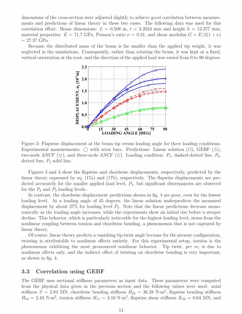
Figure 3: Flapwise displacement at the beam tip versus loading angle for three loading conditions.Experimental measurements: © with error bars. Predictions: Linear solution (✷), GEBF (△),two-node ANCF (▽), and three-node ANCF (♦). Loading condition: P1, dashed-dotted line, P2,dotted line, P3 solid line.

Figures 3 and 4 show the flapwise and chordwise displacements, respectively, predicted by thelinear theory expressed by eq. (17a) and (17b), respectively. The flapwise displacements are pre-dicted accurately for the smaller applied load level, P1, but significant discrepancies are observedfor the P2 and P3 loading levels.

In contrast, the chordwise displacement predictions shown in fig. 4 are poor, even for the lowestloading level. At a loading angle of 45 degrees, the linear solution underpredicts the measureddisplacement by about 27% for loading level P3. Note that the linear predictions decrease mono-tonically as the loading angle increases, while the experiments show an initial rise before a steeperdecline. This behavior, which is particularly noticeable for the highest loading level, stems from thenonlinear coupling between torsion and chordwise bending, a phenomenon that is not captured bylinear theory.

Of course, linear theory predicts a vanishing tip twist angle because for the present configuration,twisting is attributable to nonlinear effects entirely. For this experimental setup, torsion is thephenomenon exhibiting the most pronounced nonlinear behavior. Tip twist, per se, is due tononlinear effects only, and the indirect effect of twisting on chordwise bending is very important,as shown in fig. 4.

3.3 Correlation using GEBF

The GEBF uses sectional stiffness parameters as input data. These parameters were computedfrom the physical data given in the previous section and the following values were used: axialstiffness S = 2.84 MN, chordwise bending stiffness H22 = 36.28 N·m2, flapwise bending stiffnessH33 = 2.43 N·m2, torsion stiffness H11 = 3.10 N·m2, flapwise shear stiffness K22 = 0.64 MN, and

11

chordwise shear stiffness K33 = 0.90 MN. The stiffness parameters of the beam’s rectangular cross-section were evaluated using the three-dimensional elasticity solution developed by Bauchau andHan [48]. If the strain energy stored per unit span of the beam is evaluated with the help ofthese stiffness coefficients, it is identical to that stored in the three-dimensional structure of infinitelength. Different shear coefficients result for the beam’s flapwise and chordwise directions.

The beam was modeled with 12 four-node elements. Each node features six degrees of freedom,three displacement and three rotation components. Cubic interpolation functions were used for bothdisplacement and rotation fields. Interpolation of the rotation field is based on the interpolation ofthe relative rotation parameter vector [44]. To eliminate shear locking effects, a three-Gauss pointreduced integration scheme was used.

LOADING ANGLE [DEG]

DIS

PL

AC

EM

EN

T,

u3 [

10

-2m

]

0 15 30 45 60 75 900.0

0.4

0.8

1.2

1.6

2.0

Figure 4: Chordwise displacement at the beam tip versus loading angle for three loading conditions.Experimental measurements: © with error bars. Predictions: Linear solution (✷), GEBF (△), two-node ANCF (▽), and three-node ANCF (♦). Loading condition: P1, dashed-dotted line, P2, dottedline, P3 solid line.

The predictions of the GEBF for the three loading cases are shown in figs 3, 4, and 5 that depictthe tip flapwise displacement, chordwise displacement, and twist, respectively. For all loading casesand loading angles, excellent correlation with experiment is observed.

3.4 Correlation using two-node ANCF beam element

Next, the predictions of the two-node ANCF beam element were correlated with experimentalresults. The beam was modeled with eight two-node elements. Twelve degrees of freedom aredefined at each node and include three displacement and nine slope components that describecross-sectional rotation and deformation. As explained in section 2.3.2, each two-node elementemploys cubic and linear shape functions in the axial and transverse directions, respectively. Inthis study, the beam has a rectangular cross-section and volume integrals were performed using fullGaussian integration: four points in the axial direction and 2× 2 points over the cross-section.

The predictions the two-node ANCF beam element for the three loading cases are shown in figs 3,4, and 5 that depict tip flapwise displacement, chordwise displacement, and twist, respectively. Forthe tip flapwise displacement, the predictions are in good agreement with the measured data. Incontrast, for the tip chordwise displacement and twist, poor correlation is observed. The predictionsare close to those of linear theory, because the two-node element does not predict torsion correctly,as shown in fig 5.

12

3.5 Correlation using three-node ANCF beam element

Finally, the predictions of the three-node ANCF beam element were correlated with experimentalresults. The beam was modeled with eight three-node elements. Nine degrees of freedom are definedat each node and include three displacement and six slope components that describe cross-sectionalrotation. Each element uses quadratic and linear shape functions in the axial and transverse direc-tions, respectively. For the three-node beam, line integrals were evaluated using selective Gaussianintegration: a two-point Gauss and a three-point Lobatto integration schemes were used to integratethe strain energies defined by eqs. (4) and (15), respectively.

The predictions for the three-node ANCF beam element for the three loading cases are shown infigs 3, 4, and 5 that depict tip flapwise displacement, chordwise displacement, and twist, respectively.For all loading cases and loading angles, excellent correlation with experiment data is observed. Notethat the predictions of the three-node ANCF element are nearly identical to those of the GEBF.This is to be expected since both formulations are nearly identical.

LOADING ANGLE [DEG]

TW

IST

AN

GL

E [

10

-2 R

AD

]

0 60 900.0

1.0

2.0

4.0

6.0

7.0

Figure 5: Twist at the beam tip versus loading angle for three loading conditions. Experimentalmeasurements: © with error bars. Predictions: GEBF (△), two-node ANCF (▽), and three-nodeANCF (♦). Loading condition: P1, dashed-dotted line, P2, dotted line, P3 solid line. Note that thelinear solution predicts a vanishing twist angle.

3.6 Convergence study for the three beam elements

To further compare the three elements used in this paper, a convergence study is presented next.Four different cases will be compared: the GEBF 3-node element (i.e., with quadratic shape func-tions), the GEBF 4-node element (i.e., with cubic shape functions), the two-node ANCF element,and three-node ANCF element. For each element, simulations were run with increasingly finermeshes for loading case P3. In each case, the reference solution was selected as that obtained withthe finest mesh and relative errors with respect to the reference solutions were then obtained.

Figure 6 shows the result of the convergence study for tip flapwise displacement at loading angleθ = 0 deg and fig. 7 the corresponding results at loading angle θ = 30 deg. Finally, fig. 8 shows therelative error in tip chordwise displacement at loading angle θ = 30 deg. Note that all results arepresented on log-log plots.

As expected from the studies of Romero [16] and Bauchau et al. [18], at equal numbers ofdegrees of freedom, the predictions of the GEBF elements are more accurate than those of theANCF elements.

13

Figure 6: Relative error in the tip flapwise displacement at loading angle θ = 0 deg, loadingconditions P3: GEBF 3-node element (✷), GEBF 4-node element (⋄), two-node ANCF (▽), andthree-node ANCF (△).

Figure 7: Relative error in tip flapwise displacement at loading angle θ = 30 deg, loading conditionsP3: GEBF 3-node element (✷), GEBF 4-node element (⋄), two-node ANCF (▽), and three-nodeANCF (△).

4 Conclusions

In this paper, the accuracies of the geometrically exact beam and absolute nodal coordinate formu-lations were assessed by comparing their respective predictions against experimental data. In theexperiment, a cantilever beam was subjected to coupled flap, lag, and twist deformations.

The predictions of the two-node beam element based on the ANCF did not correlate well withthe experimental data. In fact, for the tip chordwise displacement and twist, predictions were closeto those of linear theory. These poor predictions stemmed from the inability of this formulationto capture the torsional behavior of the beam accurately. The inadequate modeling of torsionalbehavior resulted, in turn, in poor predictions of the coupled chordwise displacements that werefound to be up to 27% in error compared to experimental measurements. This two-node beamelement is rooted in the original ANCF proposed by Shabana and Yakoub. Although accuratepredictions can be obtained for planar beam problems, this study suggests that this formulationshould not be used for three-dimensional beams undergoing coupled bending and torsion.

The numerical predictions of the GEBF and of the recently proposed three-node element based

14

Figure 8: Relative error in tip chordwise displacement at loading angle θ = 30 deg, loading conditionsP3: GEBF 3-node element (✷), GEBF 4-node element (⋄), two-node ANCF (▽), and three-nodeANCF (△).

on the ANCF agree well with the experimental data at all loading angles and for the three loadingcases. Although the numerical implementations of the elements differ, both elements share thesectional strain and strain energy definitions that characterize the GEBF. The GEBF presentedhere uses a minimum set of variables, three nodal displacements and rotations. In contrast, thethree-node ANCF element uses a redundant set of coordinates: six degrees of freedom are used torepresent rotation of the cross-section. Constraints are enforced via the penalty method.

This study demonstrates the crucial need for thorough validation of the beam elements usedfor the simulation of flexible multibody systems before they are used to solve practical problems.Comparison with available experimental data seems indispensable. Predictions of the original ab-solute nodal coordinate formulation have been widely presented in the literature, primarily forplanar problems, yet this study shows that this formulation cannot handle three-dimensional beamproblems accurately.

5 Acknowledgements

The authors would like to thank the Academy of Finland (Application No. 259543) for supportingMarko K. Matikainen.

References

[1] J.C. Houbolt and G.W. Brooks. Differential equations of motion for combined flapwise bending,chordwise bending, and torsion of twisted nonuniform rotor blades. Technical Report 1348,NACA Report, 1958.

[2] D.H. Hodges and E.H. Dowell. Nonlinear equations of motion for the elastic bending andtorsion of twisted nonuniform rotor blades. Technical report, NASA TN D-7818, 1974.

[3] E.H. Dowell and J.J. Traybar. An experimental study of the nonlinear stiffness of a rotor bladeundergoing flap, lag, and twist deformations. Aerospace and Mechanical Science Report 1257,Princeton University, 1975.

15

[4] E.H. Dowell, J.J. Traybar, and D.H. Hodges. An experimental-theoretical correlation studyof non-linear bending and torsion deformations of a cantilever beam. Journal of Sound and

Vibration, 50(4):533–544, February 1977.

[5] J.C. Simo. A finite strain beam formulation. The three-dimensional dynamic problem. Part I.Computer Methods in Applied Mechanics and Engineering, 49(1):55–70, 1985.

[6] J.C. Simo and L. Vu-Quoc. A three-dimensional finite strain rod model. Part II: Computationalaspects. Computer Methods in Applied Mechanics and Engineering, 58(1):79–116, 1986.

[7] M. Borri and T. Merlini. A large displacement formulation for anisotropic beam analysis.Meccanica, 21:30–37, 1986.

[8] D.A. Danielson and D.H. Hodges. Nonlinear beam kinematics by decomposition of the rotationtensor. Journal of Applied Mechanics, 54(2):258–262, 1987.

[9] D.A. Danielson and D.H. Hodges. A beam theory for large global rotation, moderate localrotation, and small strain. Journal of Applied Mechanics, 55(1):179–184, 1988.

[10] O.A. Bauchau and C.H. Hong. Finite element approach to rotor blade modeling. Journal of

the American Helicopter Society, 32(1):60–67, 1987.

[11] O.A. Bauchau and C.H. Hong. Large displacement analysis of naturally curved and twistedcomposite beams. AIAA Journal, 25(11):1469–1475, 1987.

[12] O.A. Bauchau and C.H. Hong. Nonlinear composite beam theory. Journal of Applied Mechan-

ics, 55:156–163, March 1988.

[13] A.A. Shabana and R.A. Wehage. A coordinate reduction technique for dynamic analysis ofspatial substructures with large angular rotations. Journal of Structural Mechanics, 11(3):401–431, March 1983.

[14] O.P. Agrawal and A.A. Shabana. Application of deformable-body mean axis to flexible multi-body system dynamics. Computer Methods in Applied Mechanics and Engineering, 56(2):217–245, 1986.

[15] A.A. Shabana. Flexible multibody dynamics: Review of past and recent developments. Multi-

body System Dynamics, 1(2):189–222, June 1997.

[16] I. Romero. A comparison of finite elements for nonlinear beams: the absolute nodal coordinateand geometrically exact formulations. Multibody System Dynamics, 20:51–68, 2008.

[17] J. Gerstmayr, H. Sugiyama, and A. Mikkola. An overview on the developments of the absolutenodal coordinate formulation. In Proceedings of the Second Joint International Conference on

Multibody System Dynamics, Stuttgart, Germany, May 2012.

[18] O.A. Bauchau, S.L. Han, A. Mikkola, and M.K. Matikainen. Comparison of the absolutenodal coordinate and geometrically exact formulations for beams. Multibody System Dynamics,32(1):67–85, June 2014.

[19] O.A. Bauchau and J.I. Craig. Structural Analysis with Application to Aerospace Structures.Springer, Dordrecht, Heidelberg, London, New-York, 2009.

[20] S.P. Timoshenko. On the correction factor for shear of the differential equation for transversevibrations of bars of uniform cross-section. Philosophical Magazine, 41:744–746, 1921.

16

[21] S.P. Timoshenko. On the transverse vibrations of bars of uniform cross-section. PhilosophicalMagazine, 43:125–131, 1921.

[22] E. Reissner. The effect of transverse shear deformation on the bending of elastic plates.Zeitschrift fur angewandte Mathematik und Physik, 12:A.69–A.77, 1945.

[23] R.D. Mindlin. Influence of rotatory inertia and shear on flexural motions of isotropic elasticplates. Journal of Applied Mechanics, 18:31–38, 1951.

[24] E. Reissner. On one-dimensional finite-strain beam theory: the plane problem. Zeitschrift furangewandte Mathematik und Physik, 23:795–804, 1972.

[25] E. Reissner. On one-dimensional large-displacement finite-strain beam theory. Studies in

Applied Mathematics, 52:87–95, 1973.

[26] E. Reissner. On finite deformations of space-curved beams. Zeitschrift fur angewandte Math-

ematik und Physik, 32:734–744, 1981.

[27] L.E. Malvern. Introduction to the Mechanics of a Continuous Medium. Prentice Hall, Inc.,Englewood Cliffs, New Jersey, 1969.

[28] D.H. Hodges. Nonlinear Composite Beam Theory. AIAA, Reston, Virginia, 2006.

[29] O.A. Bauchau. Flexible Multibody Dynamics. Springer, Dordrecht, Heidelberg, London, New-York, 2011.

[30] V. Giavotto, M. Borri, P. Mantegazza, G. Ghiringhelli, V. Carmaschi, G.C. Maffioli, andF. Mussi. Anisotropic beam theory and applications. Computers & Structures, 16(1-4):403–413, 1983.

[31] O.A. Bauchau and S.L. Han. Three-dimensional beam theory for flexible multibody dynamics.Journal of Computational and Nonlinear Dynamics, 9(4):041011 (12 pages), 2014.

[32] K.E. Dufva, J.T. Sopanen, and A.M. Mikkola. A three-dimensional beam element based on across-sectional coordinate system approach. Nonlinear Dynamics, 43(4):311–327, 2005.

[33] K. Nachbagauer, P. Gruber, and J. Gerstmayr. Structural and continuum mechanics ap-proaches for a 3d shear deformable ancf beam finite element: Application to static andlinearized dynamic examples. ASME Journal of Computational and Nonlinear Dynamics,8(2):021004, 2013.

[34] A.A. Shabana and R.Y. Yakoub. Three dimensional absolute nodal coordinate formulation forbeam elements: Theory. ASME Journal of Mechanical Design, 123:606–613, 2001.

[35] R.Y. Yakoub and A.A. Shabana. Three dimensional absolute nodal coordinate formulationfor beam elements: Implementation and applications. ASME Journal of Mechanical Design,123:614–621, 2001.

[36] K. S. Kerkkanen, J. T. Sopanen, and A. M. Mikkola. A linear beam finite element based on theabsolute nodal coordinate formulation. Journal of Mechanical Design, 127(4):621–630, 2005.

[37] D. Garcıa-Vallejo, A. Mikkola, and J.L. Escalona. A new locking-free shear deformable finiteelement based on absolute nodal coordinates. Nonlinear Dynamics, 50(1-2):249–264, 2007.

17

[38] J. Gerstmayr, M.K. Matikainen, and A.M. Mikkola. A geometrically exact beam elementbased on the absolute nodal coordinate formulation. Multibody System Dynamics, 20(4):359–384, 2008.

[39] K. Nachbagauer, S.A. Pechstein, H. Irschik, and J. Gerstmayr. A new locking free formulationfor planar, shear deformable, linear and quadratic beam finite elements based on the absolutenodal coordinate formulation. Journal of Multibody System Dynamics, 26(3):245–263, 2011.

[40] M.K. Matikainen, R. von Hertzen, A.M. Mikkola, and J. Gerstmayr. Elimination of highfrequencies in the absolute nodal coordinate formulation. Proceedings of the Institution of

Mechanical Engineers, Part K: Journal of Multi-body Dynamics, 224(1):103–116, 2010.

[41] M.K. Matikainen, O. Dmitrochenko, and A.M. Mikkola. Beam elements with trapezoidal cross-section deformation modes based on the absolute nodal coordinate formulation. In International

Conference of Numerical Analysis and Applied Mathematics, Rhodes, Greece, 19-25 September2010.

[42] M.A. Crisfield and G. Jelenic. Objectivity of strain measures in the geometrically exact three-dimensional beam theory and its finite-element implementation. Proceedings of the Royal So-

ciety, London: Mathematical, Physical and Engineering Sciences, 455(1983):1125–1147, 1999.

[43] O.A. Bauchau, A. Epple, and S.D. Heo. Interpolation of finite rotations in flexible multibodydynamics simulations. Proceedings of the Institution of Mechanical Engineers, Part K: Journal

of Multi-body Dynamics, 222(K4):353–366, 2008.

[44] O.A. Bauchau and S.L. Han. Interpolation of rotation and motion. Multibody System Dynamics,31(3):339–370, 2014.

[45] P. Betsch. The discrete null space method for the energy consistent integration of constrainedmechanical systems. Part I: Holonomic constraints. Computer Methods in Applied Mechanics

and Engineering, 194(50-52):5159–5190, 2005.

[46] P. Betsch and S. Leyendecker. The discrete null space method for the energy consistent integra-tion of constrained mechanical systems. Part II: Multibody dynamics. International Journal

for Numerical Methods in Engineering, 67:499–552, 2006.

[47] S. Leyendecker, P. Betsch, and P. Steinmann. The discrete null space method for the en-ergy consistent integration of constrained mechanical systems. Part III: Flexible multibodydynamics. Multibody System Dynamics, 19(1-2):45–72, 2008.

[48] S.L. Han and O.A. Bauchau. Nonlinear three-dimensional beam theory for flexible multibodydynamics. Multibody System Dynamics, 34(3):211–242, July 2015.

18