Robotics and Autonomous Systems 54 (2006) 864–872www.elsevier.com/locate/robot

Experiments in learning distributed control for a hexapod robot

T.D. Barfoot, E.J.P. Earon, G.M.T. D’Eleuterio∗

Institute for Aerospace Studies, University of Toronto, 4925 Dufferin Street, Toronto, Ontario, Canada M3H 5T6

Received 29 June 2004; received in revised form 24 April 2006; accepted 24 April 2006Available online 28 August 2006

Abstract

This paper reports on experiments involving a hexapod robot. Motivated by neurobiological evidence that control in real hexapod insects isdistributed leg-wise, we investigated two approaches to learning distributed controllers: genetic algorithms and reinforcement learning. In the caseof reinforcement learning, a new learning algorithm was developed to encourage cooperation between legs. Results from both approaches arepresented and compared.c© 2006 Published by Elsevier B.V.

Keywords: Hexapod robot; Distributed control; Reinforcement learning; Genetic algorithm; Coevolution

1. Introduction

Insects and spiders are examples of relatively simplecreatures from nature which are able to successfully operatemany legs at once in order to navigate a diversity of terrains.Inspired by these biological marvels, robotics researchers haveattempted to mimic insect-like behaviour in legged robots [6,10]. As Schroer et al. [28] and Allen et al. [1] make clearin their work inspired by the ambulation of cockroaches, it isproductive to try and abstract biological principles which canthen motivate the engineering of a walking robot. Typically,however, the control algorithms for these types of robot arequite complicated (e.g., dynamic neural networks), requiringfairly heavy on-line computations to be performed in realtime. Here a simpler approach is presented which reduces theneed for such computations by using a coarsely coded controlscheme. This representation is suitable for our primary focus,which is to learn distributed controllers from feedback. This isan important problem in, for example, planetary exploration,where the nature of the terrain may not be known a priori andthus controllers need to be learned in situ.

Work has been done to increase the feasibility of usingsimulation to develop evolutionary control algorithms for

∗ Corresponding author.E-mail addresses: tim.barfoot@utoronto.ca (T.D. Barfoot),

e.earon@utoronto.ca (E.J.P. Earon), gabriele.deleuterio@utoronto.ca(G.M.T. D’Eleuterio).

0921-8890/$ - see front matter c© 2006 Published by Elsevier B.V.doi:10.1016/j.robot.2006.04.009

mobile robots [15,20,21,40]. It has been suggested thathardware simulation is often too time-consuming, and softwareexperimentation can accurately develop control strategiesinstead. It has been argued that the primary drawback tosoftware simulation is the difficulty in modeling hardwareinteractions in software. While adequate behaviours can beevolved [17,18] and while Jacobi [21] has developed “minimalsimulations” in order to derive such controls, it has been foundthat there are still hardware concerns that are difficult to predictusing minimal simulations (e.g. damaging current spikes in theleg drive motors) [19].

Gomi and Ide [19] use a genetic algorithm to developwalking controllers for, an octopod robot. However, ratherthan reducing the search space through preselecting a reducedset of behaviours, they very precisely shaped [13] the fitnessfunction for reinforcement. One benefit of this is that suchfitness function optimization is much more easily scaled up toallow for more complicated behaviour combinations.

What is important to note, though, is that while Gomi andIde [19] used measurements of the electric current supplied tothe leg drive motors as one feature of their fitness function, asopposed to using only the observable success of the controller(i.e., the distance walked as measured with an odometer) as isdone in the present work, the results have similar attributes.For example, behaviours that could cause a high current flowin the leg motors, such as having two or more legs in directopposition, are also behaviours that would exhibit low fitnessvalues when measuring the forward distance travelled. Thus

T.D. Barfoot et al. / Robotics and Autonomous Systems 54 (2006) 864–872 865

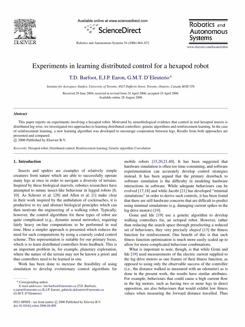
Fig. 1. (Left) Behavioural coupling between legs in stick insects [11]. (Right) Kafka, a hexapod robot, and treadmill setup designed to evolve walking gaits.

when the controllers are evolved on hardware such parametersare often taken into account by the robot itself, and modeling isnot necessarily required.

As with dynamic neural network approaches, each leg ofa robot is given its own controller rather than using a centralpattern generator. Communication between controllers is local(legs “talk” to their neighbours) resulting in a global behaviour(walking gait) for the robot. There is some neurobiologicalevidence that this notion of local control holds for somebiological insects [11]. This paradigm of interacting simpleparts has also been popular in robotics [8,9].

Støy et al. [30] have studied how identical multipleunits can be connected into a larger robotic structure whilehaving their roles automatically defined through a coordinationmechanism. Although the focus of their work is chain-typeself-reconfigurable robots, the role-based control approach hasbeen used to implement a particular type of specified gait.The controllers in our work for each leg are locally coupledbut they are not preprogrammed to produce a particular gait.Wei et al. [36] have addressed the problem of tailoring therobot’s gait based on its environment. Their robot is designedto transition passively and mechanically from a tripod gaitto an in-phase gait for climbing. While our method is alsoaimed at tailoring the gait to a robot’s environment, we relyon feedback to make active modifications to the gait. Theapproach of Wei et al. is likely better suited to high-speedlocomotion whereas the present work was motivated by suchtasks as robotic planetary exploration. We furthermore see ourbiologically motivated control approach as complementing thenonadaptive control schemes in the biologically inspired workof Schroer [28] and Allen [1] on walking robots.

The controllers used here are cellular automata (simplelookup tables). Each leg is given its own cellular automaton(CA) which can be in one of a finite number of states [34].Based on its state and those of its neighbours, a new state ischosen according to the lookup table. Each state correspondsto a fixed basis behaviour but can roughly be thought of as a

specific leg position. Thus, new leg positions are determinedby the old leg positions. Typically, all legs are updatedsynchronously such that the robot’s behaviour is represented bya set of locally coupled difference equations which are muchquicker to compute in real time than differential equations,making this approach suitable for learning.

Under this framework, design of a control algorithm isreduced to coming up with the cellular automata which producesuccessful walking gaits. We look at two approaches to do this.First, we look at genetic algorithms [4,14,16,31] in simulationand on real hardware. Second, we develop a distributedreinforcement learning approach [3,5,31] in an attempt to speedup the learning process. The paper concludes with discussionsand recommendations.

2. Controller representation

According to neurobiological evidence [11], the behaviourof legs in stick insects is locally coupled as in Fig. 1. Thispattern of ipsilateral and contralateral connections will beadopted for the purposes of discussion although any patterncould be used in general (however, only some of them wouldbe capable of producing viable walking gaits).

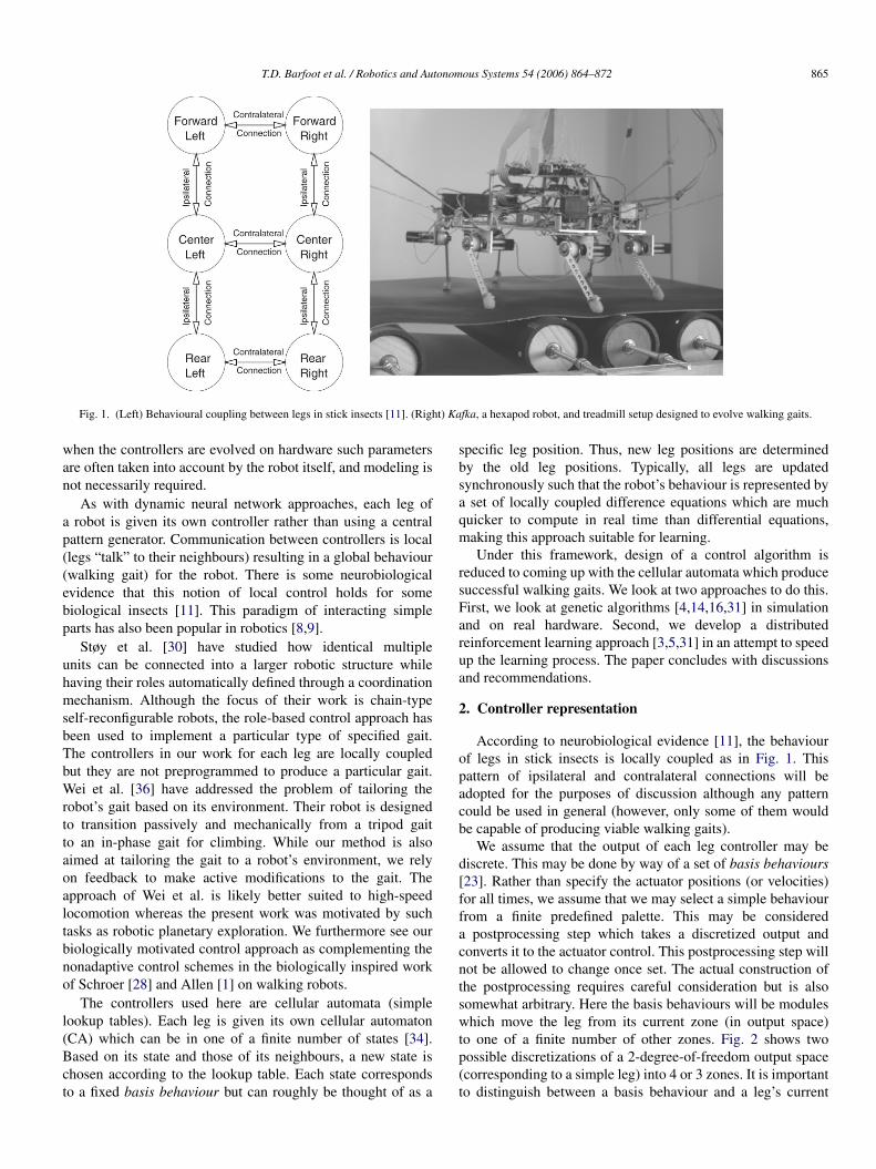
We assume that the output of each leg controller may bediscrete. This may be done by way of a set of basis behaviours[23]. Rather than specify the actuator positions (or velocities)for all times, we assume that we may select a simple behaviourfrom a finite predefined palette. This may be considereda postprocessing step which takes a discretized output andconverts it to the actuator control. This postprocessing step willnot be allowed to change once set. The actual construction ofthe postprocessing requires careful consideration but is alsosomewhat arbitrary. Here the basis behaviours will be moduleswhich move the leg from its current zone (in output space)to one of a finite number of other zones. Fig. 2 shows twopossible discretizations of a 2-degree-of-freedom output space(corresponding to a simple leg) into 4 or 3 zones. It is importantto distinguish between a basis behaviour and a leg’s current

866 T.D. Barfoot et al. / Robotics and Autonomous Systems 54 (2006) 864–872

Fig. 2. Example discretizations of output space for 2 degree of freedom legsinto (Left) 4 zones and (Right) 3 zones.

zone. If legs always arrive where they are asked to go, there islittle difference. However, in a dynamic robot moving on roughterrain, the requested leg action may not always be successful.The key difference is that the output state of a leg willcorrespond to the current basis behaviour being activated, ratherthan the leg’s current zone in output space. The input state of aleg could be either the basis behaviour or leg zone, dependingon whether one wanted to try and account for unsuccessfulrequests. By using basis behaviours, the leg controllers may beentirely discrete. Once all the postprocessing has been set up,the challenge remains to find an appropriate arbitration schemewhich takes in a discrete input state, s, (current leg positionsor basis behaviours of self and neighbours) and outputs theappropriate discrete output, a, (one of M basis behaviours)for each leg. There are several candidates for this role but theone affording the most general decision surfaces between inputand output is a straightforward lookup table similar to cellularautomata (CA).

Das et al. [12] showed that genetic algorithms were ableto evolve cellular automata which performed prescribed tasksrequiring global coordination. This is essentially what we wishto achieve but we have the added difficulty of dealing with thephysical environment of our robot. This type of lookup tablecontrol in autonomous robots is often called reactive. For everypossible input sequence the CA scheme stores a discrete outputvalue. In other words, for every possible input sequence thereis an output corresponding to one of the basis behaviours. Ateach time-step, the leg controller looks up the action whichcorresponds to its current input sequence and carries it out. Thesize of the lookup table for a leg which communicates withk − 1 other legs will then be Mk . The approach is thereforeusually rendered feasible for only modest numbers for k andM . The number of all possible lookup tables is M (Mk ). Again,modest numbers of basis behaviours keep the size of the searchspace reasonable. For example, with a hexapod robot withcoupling as in Fig. 1 and output discretization as in Fig. 2 (left)the forward and rear legs will require lookup tables of size43 and the central legs 44. If we assume left–right pairs oflegs have identical controllers the combined size of the lookuptables for forward, center, and rear legs will be 43

+ 43+

44= 384 and the number of possible table combinations for

the entire robot will be 4384. From this point on, the termCA lookup table will refer to the combined set of tables forall legs in the robot (i.e., the concatenation of individual leglookup tables).

3. Evolutionary search

The crucial step in this approach is the discovery ofparticular CA lookup tables which cause the connected legs toproduce successful walking gaits. We must discover the localrules which produce the desired global behaviour, if they indeedexist, and then find out why those rules stand out. The obviousfirst method to attempt is to design the local rules by hand.It turns out to be very difficult to do this for all but the mosttrivial examples as we are typically faced with a combinatorialexplosion. Another method is to employ an evolutionary globaloptimization technique, namely a genetic algorithm (GA), tosearch for good cellular automata [2].

GAs are based on biological evolution [16]. A randominitial population of P CA lookup tables is evolved over Ggenerations. Each CA lookup table, φ, has a chromosome whichconsists of a sequence of all the discrete values taken fromthe table. At each generation, a fitness is assigned to each CAlookup table (based on how well the robot performs on somewalking task when equipped with that CA lookup table). ACA lookup table’s fitness determines its representation in thenext generation. Genetic crossovers and mutations introducenew CA lookup tables into the population. The best K ≤ PCA lookup tables are copied exactly from one generation tothe next. The remaining (P − K ) CA lookup tables are madeup by single site crossovers where both parents are takenfrom the best K individuals. Furthermore, they are subjectedto random site mutations with probability, pm , per site. Thevariable used to determine mutation is selected from a uniformrandom distribution.

4. Example controller

In this section, the results of constructing an examplecontroller in simulation will be presented. The purpose ofthe simulation is not to model an insect robot, but rather todemonstrate that a network of cellular automata controllerscould produce patterns which resemble known walking gaits.Furthermore, we would like to show that a genetic algorithmis indeed capable of finding particular CA lookup tables whichperform well on a user defined task.

One well established gait for hexapod robots is the “tripod”gait. The legs are divided into two sets

Forward Left, Center Right, Rear Left

Forward Right, Center Left, Rear Right

While one set is on the ground, the other is lifted, swungforward, and then lowered.

For the discretization of Fig. 2 (left), there are I = 46=

4096 possible initial states for a hexapod robot. The fitness of aparticular CA lookup table will be defined as

ftotal =

I∑i=1

fi

I(1)

fi =

1 if tripod gait emerges within T time-stepsstarting from initial condition, i

0 otherwise.(2)

T.D. Barfoot et al. / Robotics and Autonomous Systems 54 (2006) 864–872 867

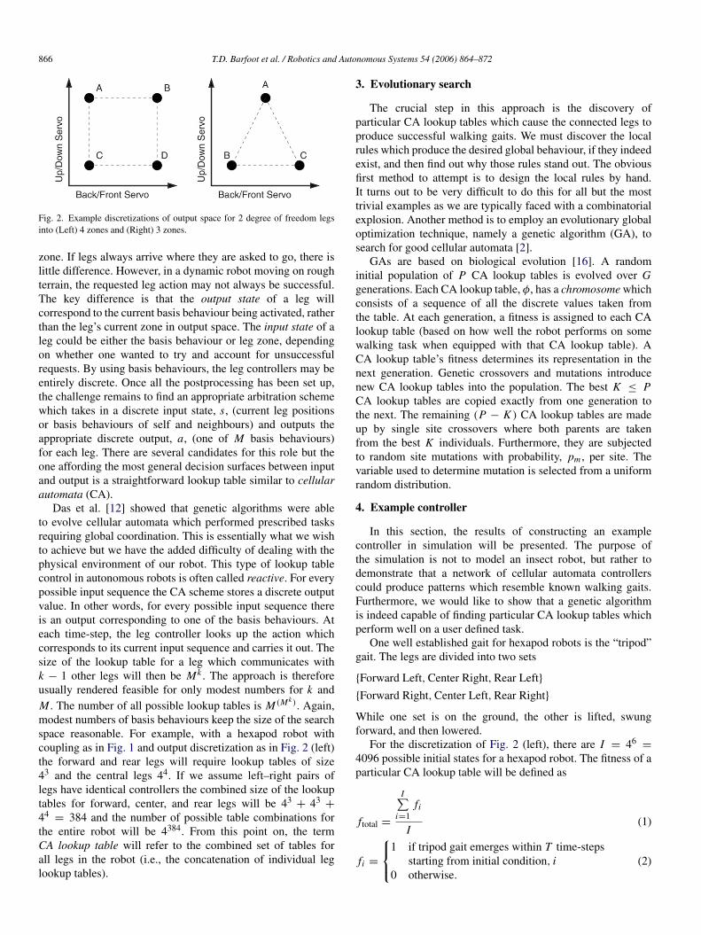
Fig. 3. (Left) Gait diagram (time history) of φtripod on a particular initial condition. Each 6-state column represents an entire leg configuration of the robot; theleft-most column is the initial condition. (Right) Attractor basin portrait of φtripod. Each node represents an entire 6-state leg configuration of the robot. Linesrepresent transitions from one leg configuration to another. The inner hexagon represents the AB DDCC . . . tripod gait.

This fitness function was used to evolve a particular CA lookuptable named φtripod, which has a fitness of 0.984. That is, from98.4% of all possible initial conditions, a tripod gait is reached.In our experiments, we have used a GA population size ofP = 50, number of generations G = 150, keepsize K = 15,and mutation probability pm = 0.005. The number of initialconditions per fitness evaluation was I = 4096 (all possibleinitial conditions) and the number of time-steps before testingfor a tripod pattern was T = 50. Fig. 3 depicts two aspects ofφtripod. The left side shows a typical gait diagram or time historyof φtripod on a particular initial condition. Each column showsthe states of the 6 legs at a given time-step (different shades ofgrey represent different leg states). The left-most column is theinitial condition. The right side is an attractor basin portrait ofφtripod as described by [39]. Each node in this plot represents anentire 6-state leg configuration of the robot (i.e., one column ofthe left plot). The inner hexagon represents the tripod gait whichis unidirectional (indicated by a clockwise arrow). The purposeof the right plot is to draw a picture of φtripod as a whole andto make a connection with the concept of stability. Beginningfrom any node on the attractor basin portrait, and following thetransitions inward (one per time-step), one will always wind upon the inner hexagon (tripod gait).

Note that only 98.4% of the 4096 possible leg configurationsare contained within the attractor basin. The remaining 1.6%of leg configurations are made up of left–right symmetricalleg configurations which can never lead to a non-symmetricalconfiguration since identical controllers have been used forleft–right pairs of legs. For a real robot this could be a problembut we will not go into the matter too deeply. Possible solutionsare to use non-identical controllers for left–right pairs of legs,to occasionally mutate individual leg states randomly (thus

breaking the symmetry), or to use asynchronous updating oflegs.

The conclusion we may draw from this simple exerciseis that this type of distributed controller certainly is able toproduce patterns resembling known walking gaits and thatgenetic algorithms are capable of finding them. The questionwe would now like to answer is whether a robot could actuallylearn such a controller from very simple feedback.

5. Evolutionary experiments

In this section we describe the results of coevolvingdistributed controllers on hardware. Fig. 1 shows Kafka [24],a hexapod robot, mounted on a treadmill. Kafka’s legs arepowered by twelve JR Servo NES 4721 hobby servomotorscontrolled by a 386 66 MHz PC, which was more than sufficientfor the purposes of this experiment. The control signals to theservos are absolute positions to which the servos then move asfast as possible. In order to control the speed of the leg motions,the path of the leg is broken down into many segments andthe legs are commanded through each of these. The fewer theintervening points, the faster the legs move.

The robot has been mounted on an unmotorized treadmillin order to automatically measure controller performance (forwalking in a straight line only). As Kafka walks, the belton the treadmill causes the rollers to rotate. An odometerreading from the rear roller is fed to Kafka’s computer suchthat distance versus time-step plots may be used to determinethe performance of the controller. The odometer measures netdistance travelled.

For this experiment, the states for Kafka’s legs wereconstrained to move only in a clockwise, forward motion which

868 T.D. Barfoot et al. / Robotics and Autonomous Systems 54 (2006) 864–872

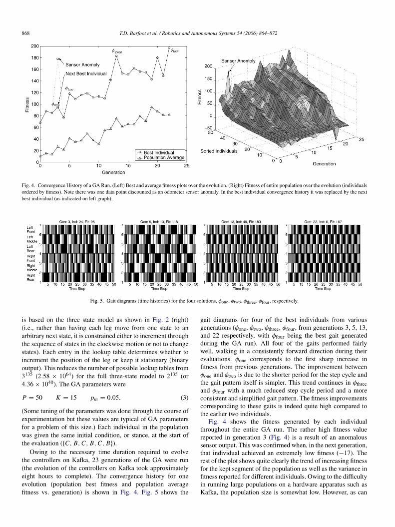
Fig. 4. Convergence History of a GA Run. (Left) Best and average fitness plots over the evolution. (Right) Fitness of entire population over the evolution (individualsordered by fitness). Note there was one data point discounted as an odometer sensor anomaly. In the best individual convergence history it was replaced by the nextbest individual (as indicated on left graph).

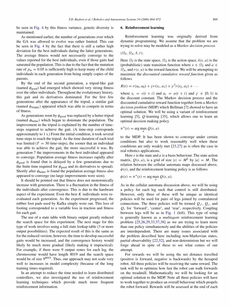
Fig. 5. Gait diagrams (time histories) for the four solutions, φone, φtwo, φthree, φfour, respectively.

is based on the three state model as shown in Fig. 2 (right)(i.e., rather than having each leg move from one state to anarbitrary next state, it is constrained either to increment throughthe sequence of states in the clockwise motion or not to changestates). Each entry in the lookup table determines whether toincrement the position of the leg or keep it stationary (binaryoutput). This reduces the number of possible lookup tables from3135 (2.58 × 1064) for the full three-state model to 2135 (or4.36× 1040). The GA parameters were

P = 50 K = 15 pm = 0.05. (3)

(Some tuning of the parameters was done through the course ofexperimentation but these values are typical of GA parametersfor a problem of this size.) Each individual in the populationwas given the same initial condition, or stance, at the start ofthe evaluation (C, B, C, B, C, B).

Owing to the necessary time duration required to evolvethe controllers on Kafka, 23 generations of the GA were run(the evolution of the controllers on Kafka took approximatelyeight hours to complete). The convergence history for oneevolution (population best fitness and population averagefitness vs. generation) is shown in Fig. 4. Fig. 5 shows the

gait diagrams for four of the best individuals from variousgenerations (φone, φtwo, φthree, φfour, from generations 3, 5, 13,and 22 respectively, with φfour being the best gait generatedduring the GA run). All four of the gaits performed fairlywell, walking in a consistently forward direction during theirevaluations. φone corresponds to the first sharp increase infitness from previous generations. The improvement betweenφone and φtwo is due to the shorter period for the step cycle andthe gait pattern itself is simpler. This trend continues in φthreeand φfour with a much reduced step cycle period and a moreconsistent and simplified gait pattern. The fitness improvementscorresponding to these gaits is indeed quite high compared tothe earlier two individuals.

Fig. 4 shows the fitness generated by each individualthroughout the entire GA run. The rather high fitness valuereported in generation 3 (Fig. 4) is a result of an anomaloussensor output. This was confirmed when, in the next generation,that individual achieved an extremely low fitness (−17). Therest of the plot shows quite clearly the trend of increasing fitnessfor the kept segment of the population as well as the variance infitness reported for different individuals. Owing to the difficultyin running large populations on a hardware apparatus such asKafka, the population size is somewhat low. However, as can

T.D. Barfoot et al. / Robotics and Autonomous Systems 54 (2006) 864–872 869

be seen in Fig. 4 by this fitness variance, genetic diversity ismaintained.

As mentioned earlier, the number of generations over whichthe GA was allowed to evolve was rather limited. This canbe seen in Fig. 4 by the fact that there is still a rather highdeviation for the best individuals during the latter generations.The average fitness would not necessarily converge to thevalues reported for the best individuals, even if those gaits hadsaturated the population. This is due to the fact that the mutationrate of pm = 0.05 is sufficiently high to keep many of the childindividuals in each generation from being simply copies of theparents.

By the end of the second generation, a tripod-like gait(named φgood) had emerged which showed very strong fitnessover the other individuals. Throughout the evolutionary history,this gait and its derivatives dominated. For the first fewgenerations after the appearance of the tripod, a similar gait(named φsloppy) appeared which was able to compete in termsof fitness.

As generations went by φgood was replaced by a better tripod(named φbetter) which began to dominate the population. Theimprovement in the tripod is explained by the number of time-steps required to achieve the gait. (A time-step correspondsapproximately to 1 s.) From the initial condition, it took severaltime-steps to reach the tripod. As the time duration of each trialwas limited (T = 30 time-steps), the sooner that an individualwas able to achieve the gait, the more successful it was. Bygeneration 7 the improvements in the best individual appearedto converge. Population average fitness increases rapidly afterφgood is found (but is delayed by a few generations due tothe finite time required for φgood and its derivatives to spread).Shortly after φbetter is found the population average fitness alsoappeared to converge (no large improvements were seen).

It should be pointed out that fitness does not monotonicallyincrease with generation. There is a fluctuation in the fitness ofthe individuals after convergence. This is due to the hardwareaspect of the experiment. Even the best K individuals were re-evaluated each generation. As the experiment progressed, therubber foot pads used by Kafka simply wore out. This loss offooting corresponded to a variable loss in traction and fitnessfor each gait.

The use of a state table with binary output greatly reducedthe search space for this experiment. The next stage for thistype of work involves using a full state lookup table (3 or moreoutput possibilities). The expected result of this is the same asfor the reduced version; however, the time to develop successfulgaits would be increased, and the convergence history wouldlikely be much more gradual (likely making it impractical).For example, if there were 9 output zones for each leg, thechromosome would have length 8019 and the search spacewould be of size 98019. Thus, our approach may not scale verywell to increases in model complexity (because of the longtraining times required).

In an attempt to reduce the time needed to learn distributedcontrollers, we also investigated the use of reinforcementlearning techniques which provide much more frequentreinforcement information.

6. Reinforcement learning

Reinforcement learning was originally derived fromdynamic programming. We assume that the problem we aretrying to solve may be modeled as a Markov decision process

(ΩS,ΩA, δ, r).

Here ΩS is the state space, ΩA is the action space, δ(s, a) is the(probabilistic) state transition function where s ∈ ΩS and a ∈ΩA, and r(s, a) is the reward function. We will be attempting tomaximize the discounted cumulative reward function given asfollows

R(t) = r(s0, a0)+ γ r(s1, a1)+ γ 2r(s2, a2)+ · · ·

where si = s(t + i) and ai = a(t + i) and γ ∈ [0, 1) isthe discount constant. The Markov decision process and thediscounted cumulative reward function together form a Markovdecision problem (MDP) which Bellman [7] showed to have anoptimal solution. We will be using a variant of reinforcementlearning [5], Q-learning [35], which allows one to learn anoptimal decision making policy

π∗(s) = arg maxa

Q(s, a)

to the MDP. It has been shown to converge under certainconditions but also to work reasonably well when theseconditions are only weakly met [23,27] as is often the case inreal robotics applications.

Here s is the state and a is a basis behaviour. The state actionmatrix, Q(s, a), is a grid of size |s| = Mk by |a| = M . Therelation between the cellular automata maps discussed above,φ(s), and the reinforcement learning policy is as follows

φ(s) = π∗(s) = arg maxa

Q(s, a).

As in the cellular automata discussion above, we will be usinga policy for each leg such that control is still distributed.However, only three of these will be unique as identicalpolicies will be used for pairs of legs joined by contralateralconnections. The three policies will be termed Q f , Qc, andQr for ‘forward’, ‘center’, and ‘rear’, respectively. Couplingbetween legs will be as in Fig. 1 (left). This type of setupis generally known as a multiagent reinforcement learningproblem [25,26,29,33,37,38] as we are trying to learn morethan one policy simultaneously and the abilities of the policiesare interdependent. There are many issues associated withthe problem described here including non-Markovian states,partial observability [22,32], and non-determinism but we willforge ahead in spite of these to see what comes of ourattempt.

For rewards we will be using the net distance travelled(positive is forward, negative is backwards) by the hexapodrobot. All three policies will be receiving the same reward. Thetask will be to optimize how fast the robot can walk forwardson the treadmill. Mathematically we will be looking for anoptimal solution to the MDP. Note all three policies will haveto work together to produce an overall behaviour which propelsthe robot forward. Rewards will be assessed at the end of each

870 T.D. Barfoot et al. / Robotics and Autonomous Systems 54 (2006) 864–872

action taken (each “step” of the robot). Typically in Q-learning,each policy is updated according to

Q(s, a)← r(s, a)+ γ maxa′

Q(s′, a′)

where s = s(t) is the old state, s′ = s(t + 1) is the new state,and r(s, a) is the reward for starting at s and selecting action a.

Unfortunately, this algorithm does not suffice for ourpurposes as we are working with a multiagent system wherethe reward is based on the performance of the entire system (notjust one leg). Specifically, the reward depends on the actions ofall six legs, not just one of them and as a result, a leg couldreceive very different values for the reward associated withfollowing an action from a given state, r(s, a) (depending onwhat the other legs decide). It does not make sense to averagethe rewards (as in stochastic Q-learning) as this can lead tosuboptimal policies.

Instead, we introduce a memory that keeps track of the bestreward earned by following action a from state s,

rmax(s, a)

which has the same dimensions as Q(s, a). We call the modifiedlearning algorithm, cooperative Q-learning, as it promotescooperation between concurrent learners (who are receivingidentical rewards). The cooperative Q-learning algorithm is asfollows

rmax(s, a)← max[rmax(s, a), r(s, a)]

Q(s, a)← rmax(s, a)+ γ maxa′

Q(s′, a′)

where s = s(t), a = a(t), s′ = s(t + 1).

7. Reinforcement learning experiments

This section briefly describes implementation of the abovealgorithm. The experiment setup is identical to that of theevolutionary experiments described above.

Cooperative Q-learning was tested on Kafka using the legcoupling of Fig. 1 (left) and the leg discretization of Fig. 2(right). To keep the size of the search space small, only twoactions were permitted for each leg: (stay in the current state)or (move one state forward in the counter-clockwise cycle,ABC ABC ABC . . .). Furthermore, the learning occurred in anepisodic manner. An episode consisted of starting the robot inthe configuration BC BC BC and allowing it 10 time-steps tochoose actions. A typical run consisted of 300 episodes. Thisepisodic-style training sped up the experiment by allowing therobot to only learn part of the Q-matrix rather than learning itin its entirety.

The last issue to discuss is the trade-off between explorationof new actions and exploitation of the best known actions.Typically in Q-learning, new actions are explored with someprobability, pexplore, otherwise the best action is chosenaccording to the Q-matrix. Here we used a linear time-varyingpexplore as depicted in Fig. 6 (bottom). This allowed manynew actions to be explored initially and fewer later on. Thisis of course a heuristic, which often needs to be “tuned” in Q-learning experiments.

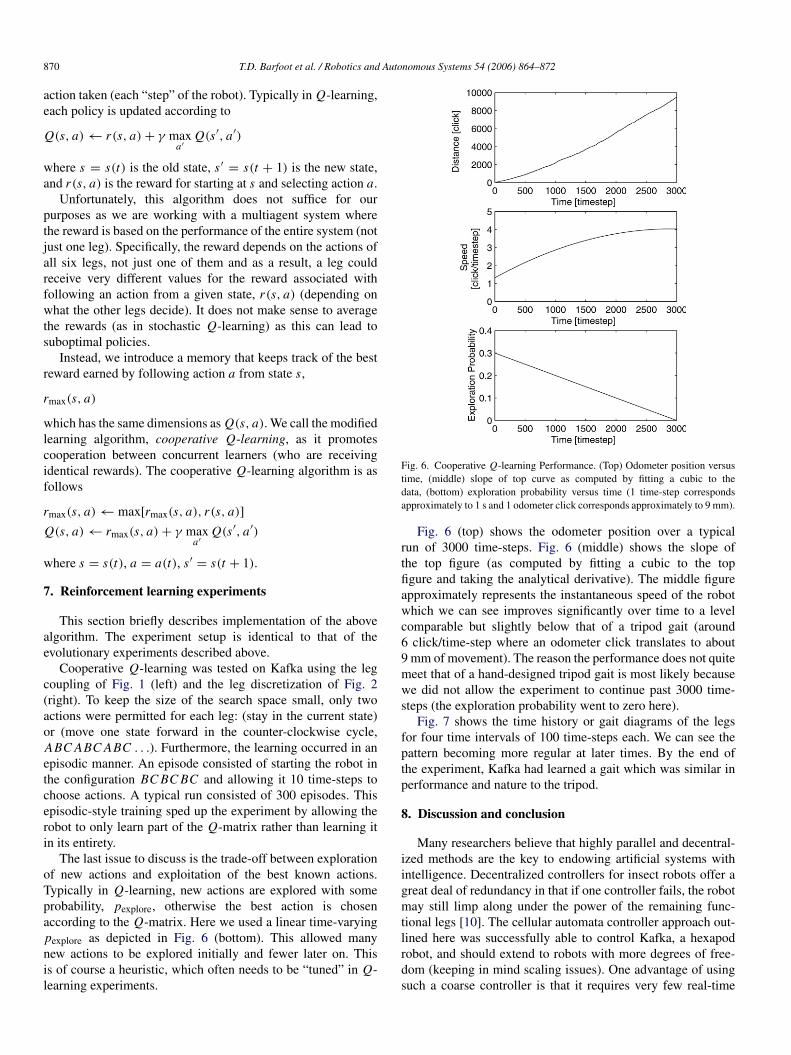
Fig. 6. Cooperative Q-learning Performance. (Top) Odometer position versustime, (middle) slope of top curve as computed by fitting a cubic to thedata, (bottom) exploration probability versus time (1 time-step correspondsapproximately to 1 s and 1 odometer click corresponds approximately to 9 mm).

Fig. 6 (top) shows the odometer position over a typicalrun of 3000 time-steps. Fig. 6 (middle) shows the slope ofthe top figure (as computed by fitting a cubic to the topfigure and taking the analytical derivative). The middle figureapproximately represents the instantaneous speed of the robotwhich we can see improves significantly over time to a levelcomparable but slightly below that of a tripod gait (around6 click/time-step where an odometer click translates to about9 mm of movement). The reason the performance does not quitemeet that of a hand-designed tripod gait is most likely becausewe did not allow the experiment to continue past 3000 time-steps (the exploration probability went to zero here).

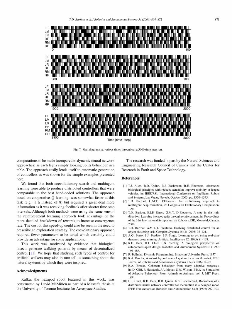
Fig. 7 shows the time history or gait diagrams of the legsfor four time intervals of 100 time-steps each. We can see thepattern becoming more regular at later times. By the end ofthe experiment, Kafka had learned a gait which was similar inperformance and nature to the tripod.

8. Discussion and conclusion

Many researchers believe that highly parallel and decentral-ized methods are the key to endowing artificial systems withintelligence. Decentralized controllers for insect robots offer agreat deal of redundancy in that if one controller fails, the robotmay still limp along under the power of the remaining func-tional legs [10]. The cellular automata controller approach out-lined here was successfully able to control Kafka, a hexapodrobot, and should extend to robots with more degrees of free-dom (keeping in mind scaling issues). One advantage of usingsuch a coarse controller is that it requires very few real-time

T.D. Barfoot et al. / Robotics and Autonomous Systems 54 (2006) 864–872 871

Fig. 7. Gait diagrams at various times throughout a 3000 time-step run.

computations to be made (compared to dynamic neural networkapproaches) as each leg is simply looking up its behaviour in atable. The approach easily lends itself to automatic generationof controllers as was shown for the simple examples presentedhere.

We found that both coevolutionary search and multiagentlearning were able to produce distributed controllers that werecomparable to the best hand-coded solutions. The approachbased on cooperative Q-learning, was somewhat faster at thistask (e.g., 1 h instead of 8) but required a great deal moreinformation as it was receiving feedback after shorter time-stepintervals. Although both methods were using the same sensor,the reinforcement learning approach took advantage of themore detailed breakdown of rewards to increase convergencerate. The cost of this speed-up could also be seen in the need toprescribe an exploration strategy. The coevolutionary approachrequired fewer parameters to be tuned which certainly couldprovide an advantage for some applications.

This work was motivated by evidence that biologicalinsects generate walking patterns by means of decentralizedcontrol [11]. We hope that studying such types of control forartificial walkers may also in turn tell us something about thenatural systems by which they were inspired.

Acknowledgments

Kafka, the hexapod robot featured in this work, wasconstructed by David McMillen as part of a Master’s thesis atthe University of Toronto Institute for Aerospace Studies.

The research was funded in part by the Natural Sciences andEngineering Research Council of Canada and the Center forResearch in Earth and Space Technology.

References

[1] T.J. Allen, R.D. Quinn, R.J. Bachmann, R.E. Ritzmann, Abstractedbiological principles with reduced actuation improve mobility of leggedvehicles, in: IEEE/RSL International Conference on Intelligent Robotsand Systems, Las Vegas, Nevada, October 2003, pp. 1370–1375.

[2] T.D. Barfoot, G.M.T. D’Eleuterio, An evolutionary approach tomultiagent heap formation, in: Congress on Evolutionary Computation,1999.

[3] T.D. Barfoot, E.J.P. Earon, G.M.T. D’Eleuterio, A step in the rightdirection: Learning hexapod gaits through reinforcement, in: Proceedingsof the 31st International Symposium on Robotics, ISR, Montreal, Canada,2000.

[4] T.D. Barfoot, G.M.T. D’Eleuterio, Evolving distributed control for anobject clustering task, Complex Systems 15 (3) (2005) 95–121.

[5] A.G. Barto, S.J. Bradtke, S.P. Singh, Learning to act using real-timedynamic programming, Artificial Intelligence 72 (1995) 81–138.

[6] R.D. Beer, H.J. Chiel, L.S. Sterling, A biological perspective onautonomous agent design, Robotics and Autonomous Systems 6 (1990)169–186.

[7] R. Bellman, Dynamic Programming, Princeton University Press, 1957.[8] R.A. Brooks, A robust layered control system for a mobile robot, IEEE

Journal of Robotics and Autonomous Systems RA-2 (1986) 14–23.[9] R.A. Brooks, Coherent behaviour from many adaptive processes,

in: D. Cliff, P. Husbands, J.A. Meyer, S.W. Wilson (Eds.), in: Simulationof Adaptive Behaviour: From Animals to Animats, vol. 3, MIT Press,1994.

[10] H.J. Chiel, R.D. Beer, R.D. Quinn, K.S. Espenschied, Robustness of adistributed neural network controller for locomotion in a hexapod robot,IEEE Transactions on Robotics and Autonomation 8 (3) (1992) 292–303.

872 T.D. Barfoot et al. / Robotics and Autonomous Systems 54 (2006) 864–872

[11] H. Cruse, Coordination of leg movement in walking animals,in: J.A. Meyer, S. Wilson (Eds.), Simulation of Adaptive Behaviour: FromAnimals to Animats, MIT Press, 1990.

[12] R. Das, J.P. Crutchfield, M. Mitchell, J.E. Hanson, Evolving globallysynchronized cellular automata, in: L.J. Eshelman (Ed.), Proceedings ofthe Sixth International Conference on Genetic Algorithms, San Fransisco,CA, 1995, pp. 336–343.

[13] M. Dorigo, M. Colombetti, Robot Shaping: An Experiment in BehaviorEngineering (Intelligent Robotics and Autonomous Agents), in: ABradford Book, MIT Press, Cambridge, MA, 1998.

[14] E.J.P. Earon, T.D. Barfoot, G.M.T. D’Eleuterio, From the sea to thesidewalk: The evolution of hexapod walking gaits by a genetic algorithm,in: Proceedings of the Third International Conference on EvolvableSystems, Edinburgh, Scotland, 2000.

[15] S. Nolfi, D. Floreano, Evolutionary Robotics: The Biology, Intelligence,and Technology of Self-Organizing Machines (Intelligent Robotics andAutonomous Agents), in: A Bradford Book, MIT Press, Cambridge, MA,2000.

[16] D.E. Goldberg, Genetic Algorithms in Search, Optimization, and MachineLearning, Addison-Wesley Pub. Co., Reading, MA, 1989.

[17] T. Gomi, A. Griffith, Evolutionary robotics — an overview, in: Proceed-ings of IEEE International Conference on Evolutionary Computation,1996, pp. 40–49.

[18] T. Gomi, Practical applications of behaviour-based robotics: The first fiveyears, in: IECON98, Proceedings of the 24th Annual Conference of theIEEE, vol. 4, Industrial Electronics Society, 1998, pp. 159–164.

[19] T. Gomi, K. Ide, Evolution of gaits of a legged robot, in: The 1998 IEEEInternational Conference on Fuzzy Systems, vol. 1, IEEE World Congresson Computational Intelligence, 1998, pp. 159–164.

[20] F. Gruau, Automatic definition of modular neural networks, AdaptiveBehaviour 3 (2) (1995) 151–184.

[21] N. Jakobi, Runnig across the reality gap: Octopod locomotion evolved ina minimal simulation, in: P. Husbands, J.-A. Meyer (Eds.), Proceedings ofEvorob98, Evorob98, Springer-Verlag, 1998.

[22] L.P. Kaebling, M.L. Littman, A.R. Cassandra, Planning and acting inpartially observable stochastic domains, Artificial Intelligence (1998) 101.

[23] M.J. Mataric, Behaviour-based control: Examples from navigation, learn-ing, and group behaviour, in: H. Hexmoor, I. Horswill, D. Kortenkamp(Eds.), Software Architectures for Physical Agents, Journal of Experimen-tal and Theoretical Artificial Intelligence 9 (2) (1997) 232–336 (specialissue).

[24] D.R. McMillen, Kafka: A hexapod robot. Master’s Thesis, University ofToronto Institute for Aerospace Studies, 1995.

[25] L. Peshkin, K.-E. Kim, N. Meuleau, L.P. Kaelbling, Learning to cooperatevia policy search, in: Proceedings of the 16th International Conference onUncertainty in AI, 2000.

[26] J. Schmidhuber, Reinforcement learning in markovian and non-markovianenvironments, in: D.S. Lippman, J.E. Moody, D.S. Touretzky (Eds.),Advances in Neural Information Processing Systems, vol. 3, MorganKaufmann, 1991, pp. 500–506.

[27] K.T. Simsarian, M.J. Mataric, Learning to cooperate using two six-legged mobile robots, in: Proceedings of the Third European Workshopof Learning Robots, Herkalion, Crete, Greece, 1995.

[28] R.T. Schroer, M.J. Boggess, R.J. Bachmann, R.D. Quinn, R.E. Ritzmann,Comparing cockroach and whegs robot body motion, in: Proceedings ofthe IEEE International Conference on Robotics and Automation, April2004, New Orleans, Lousiana, 2004, pp. 3288–3293.

[29] P. Stone, Layered Learning in Multiagent Systems: A Winning Approachto Robotic Soccer, MIT Press, Cambridge, MA, 2000.

[30] K. Støy, W.-M. Shen, P.M. Will, Using role-based control to producelocomotion in chain-type reconfigurable robots, IEEE Transactions onMechatronics 7 (4) (2002) 410–417.

[31] R.S. Sutton, A.G. Barto, Reinforcement Learning: An Introduction, in: ABradford Book, MIT Press, 1998.

[32] S. Thrun, Monte carlo pomdps, in: Proceedings of Conference on NeuralInformation Processing Systems, NIPS, 1999.

[33] C. Versino, L.M. Gambardella, Learning real team solutions, in: G. Weib(Ed.), Distributed Artificial Intelligence Meets Machine Learning,Springer, 1997, pp. 40–61.

[34] J. von Neumann, Theory of Self-reproducing automata, University ofIllinois Press, Urbana and London, 1966.

[35] C.J.C.H. Watkins, Learning from delayed rewards, Ph.D. Thesis,Cambridge University, Cambridge, England, 1989.

[36] T.E. Wei, R.D. Quinn, R.E. Ritzmann, A CLAWAR That benefits fromabstracted cockroach locomotion principles, in: Proceedings of the 7thInternational Conference on Climbing and Walking Robots, September2004, Madrid, Spain, 2004.

[37] G. Weiss (Ed.), Multiagent Systems: A Modern Approach to DistributedArtificial Intelligence, MIT Press, Cambridge, MA, 1999.

[38] L.F.A. Wessels, Multiagent reinforcement learning, Ph.D. Thesis, Facultyof Engineering, University of Pretoria, 1997.

[39] A. Wuensche, The ghost in the machine: Basins of attraction of randomboolean networks, in: C.G. Langton (Ed.), Artificial Life III: SFI Studiesin the Sciences of Complexity, vol. XVII, Addison-Wesley, 1994.

[40] D. Zeltzer, M. McKenna, Simulation of autonomous legged locomotion,in: C.G. Langton (Ed.), Artificial Life III: SFI Studies in the Sciences ofComplexity, vol. XVII, Addison-Wesley, 1994.

T.D. Barfoot is currently working in the Controls andAnalysis Group at MDA Space Missions. Previously,he was an Assistant Professor in the Space RoboticsGroup at the University of Toronto Institute forAerospace Studies. He received his B.A.Sc. in theAerospace Option of Engineering Science at theUniversity of Toronto. His Ph.D. Thesis, obtained fromthe Institute for Aerospace Studies at the Universityof Toronto, focused on the coordination of multiple

mobile robots. His current research interests lie in the area of experimentalmobile robotics for both space and terrestrial applications.

E.J.P. Earon received his B.A.Sc. in AerospaceEngineering at the University of Toronto in 1999and began his doctoral research at the University ofToronto Institute for Aerospace Studies. His researchcentred on robotic control and flexible, adaptablemachine learning topics with particular emphasis onevolutionary and genetic computation. He received hisPh.D. in 2005.

G.M.T. D’Eleuterio was born in Teramo, Italy.He received his B.A.Sc. in Engineering Science(Aerospace) from the University of Toronto and hisM.A.Sc. and Ph.D. from the University of TorontoInstitute for Aerospace Studies. His current researchinterests include space robotics and biologicallyinspired approaches to robotic control. He is aProfessor at the University of Toronto Institute forAerospace Studies.