Experiments on extreme wave generationusing the Soliton on Finite Background

Rene H.M. Huijsmans1, Gert Klopman2,3, Natanael Karjanto3, andAndonawati4

1 Maritime Research Institute Netherlands, Wageningen, The Netherlands,e-mail: r.h.m.huijsmans@marin.nl

2 Albatros Flow Research, Marknesse, The Netherlands3 Applied Analysis and Math. Physics, Univ. of Twente, Enschede, The Netherlands

4 Jurusan Matematika, Institut Teknologi Bandung, Bandung, Indonesia

Introduction

Freak waves are very large water waves whose heights exceed the significant waveheight of a measured wave train by a factor of more than 2.2. However, this initself is not a well established definition of a freak wave. The mechanism of freakwave generation in reality as well as modeling it in a wave basin has become anissue of great importance.Recently one is aware of the generation of freak wave through the Benjamin–Feirtype of instability or self–focussing. Consequently the Non–Linear–Schrodinger(NLS) equation forms a good basis for understanding the formation of freakwaves. However, the complex generation of a freak wave in nature within a seacondition is still not well understood, when the non-linearity of the carrier waveis not small. In our study we will focus on the Soliton on Finite Background,an exact solution of the NLS equation, as a generating mechanism for extremewaves.Apart from a numerical investigation into the evolution of a soliton on a fi-nite background also extensive detailed model tests have been performed forvalidation purposes in the hydrodynamic laboratories of the Maritime ResearchInstitute Netherlands (marin). Furthermore, a numerical wave tank [12] is usedto model the complete non-linear non-breaking wave evolution in the basin.

Properties of the Soliton on Finite Background

The NLS equation is chosen as a mathematical model for the non-linear evolutionof the envelope of surface wave packets. For spatial evolution problems, it is givenin non-dimensional form and in a frame of reference moving with the groupvelocity by

∂ξψ + iβ∂2τψ + iγ|ψ|2ψ = 0, (1)

where ξ and τ are the corresponding spatial and temporal variables, respectively;β and γ are the dispersion and non-linearity coefficients. This equation has many

2

families of exact solutions. One family of exact solutions is known as the Solitonon Finite Background (SFB) and this is a good candidate for describing extremewaves. This exact solution has been found by Akhmediev, Eleonskii & Kulagin[3], see also [2] and [1].

This SFB solution describes the dynamic evolution of an unstable modu-lation process, with dimensionless modulation frequency ν. In the context ofwater waves, for infinitesimal modulational perturbations to a finite-amplitudeplane wave, this process is known as Benjamin-Feir (BF) instability [5]. How-ever, non-linearity will limit this exponential growth and the SFB is one (ofmany other) non-linear extension of the BF instability for larger amplitudes ofthe modulation. Extensive research on the NLS equation and the SFB solution,to obtain a better understanding of deterministic extreme-wave phenomena hasbeen conducted in the past few years (see e.g. [10], [11], [4] and [9]).

An explicit expression for the SFB is given as the following complex-valuedfunction

ψ(ξ, τ ; ν, r0) = A(ξ) ·

ν2 cosh(σξ)− i[σ/(γr20)

]sinh(σξ)

cosh(σξ)−√

1− 12 ν

2 cos(ντ)− 1

, (2)

where A(ξ) = r0e−iγr2

0ξ is the plane-wave or the continuous wave solution of theNLS equation, σ = γr20 ν

√2− ν2 is the growth rate corresponds to the Benjamin-

Feir instability, ν = ν r0√

γβ is the modulation frequency, and ν, 0 < ν <

√2 is

the normalized modulation frequency. This SFB reaches its maxima at (ξ, τ) =(0, 2nπ

ν

), n ∈ Z. It has a soliton-like form with a finite background in the spatial

ξ-direction. The SFB is periodic along in the temporal τ -direction, with period2πν . For |ξ| → ∞, the SFB turns into the continuous wave solution A(ξ). It

possesses two essential parameters: r0 and ν.

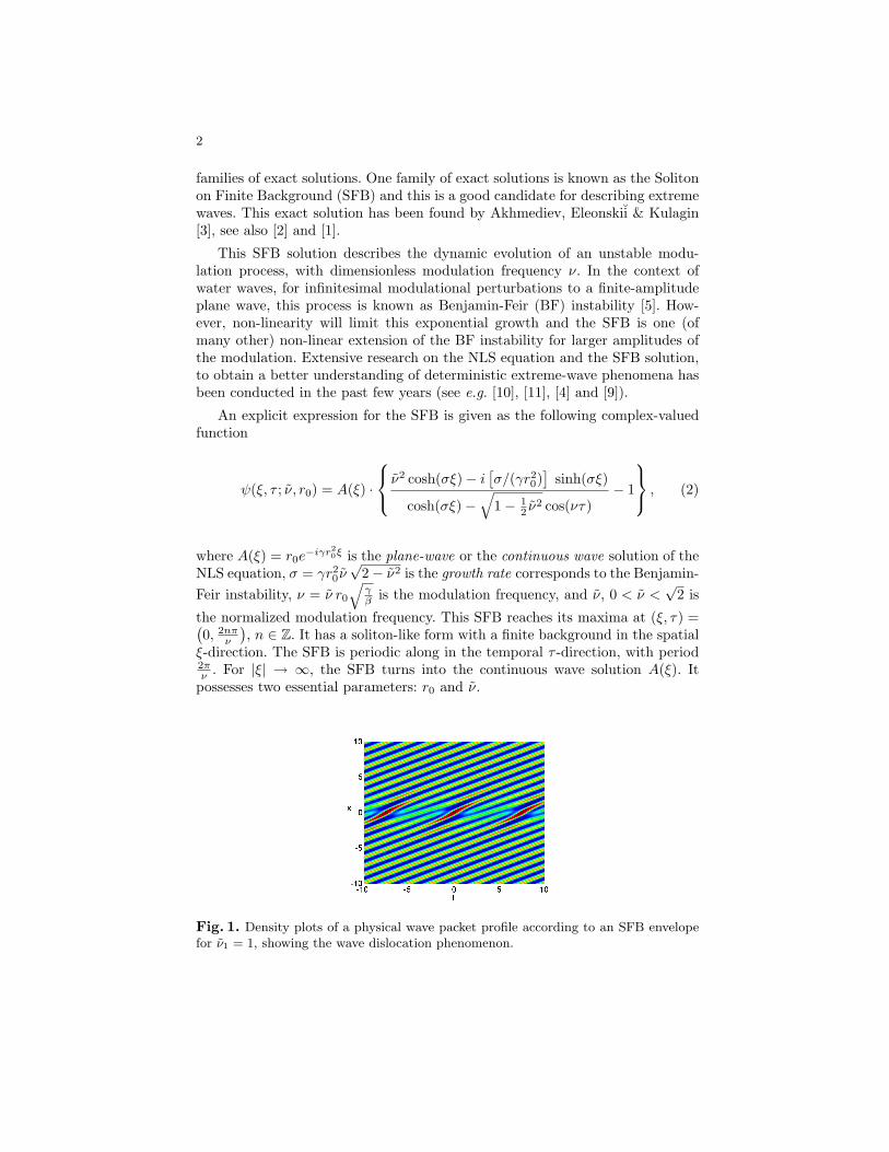
Fig. 1. Density plots of a physical wave packet profile according to an SFB envelopefor ν1 = 1, showing the wave dislocation phenomenon.

3

The first-order part of the corresponding physical wave packet profile η(x, t)for a given complex-valued function ψ(ξ, τ) is expressed as follows

η(x, t) = ψ(ξ, τ)ei(k0x−ω0t) + c.c., (3)

where c.c. means the complex conjugate of the preceding term, the wave numberk0 and frequency ω0 satisfy the linear dispersion relation ω = Ω(k) ≡

√k tanh k.

The variables (x, t) in the non-moving frame of reference are related to (ξ, τ) inthe moving frame of reference by the transformation ξ = x and τ = t−x/Ω′(k0).The modulus of ψ represents the wave group envelope, enclosing the wave packetprofile η(x, t). The dimensional laboratory quantities are related to the non-dimensional quantities by the following Froude scaling, using the gravitionalacceleration g and the depth of the basin h: xlab = x·h, tlab = t·

√gh , klab = k/h,

ωlab = ω ·√

gh , and ηlab = η · h.

In principle, the wave profile including the higher-order terms represents agood approximation to the situation in real life. To accommodate this fact, wewill include higher-order terms up to second order. We apply an perturbation-series expansion (Stokes’ expansion) to the physical wave-packet profile η(x, t)and the multiple-scale approach using the variables ξ and τ , where ξ = ε2x, τ =ε(t−x/Ω′(k0)), and ε is a small positive non-linearity and modulation parameter.The corresponding wave elevation η(x, t), consisting of the superposition of thefirst-order harmonic term of O(ε) and a second-order non-harmonic long waveas well as a second-order double-frequency harmonic term of O(ε2), is given by

η(x, t) = ε[ψ(10)(ξ, τ)ei(k0x−ω0t) + c.c.

]+ ε2

ψ(20)(ξ, τ) +

[ψ(22)(ξ, τ)e2i(k0x−ω0t) + c.c.

]. (4)

We find from the multiple-scales perturbation-series approach that ψ(10)(ξ, τ) =ψ(ξ, τ) satisfies the spatial NLS equation and

ψ(20)(ξ, τ) = − 1Ω(k0)

4k0Ω′(k0)−Ω(k0)

[Ω′(0)]2 − [Ω′(k0)]2|ψ(10)(ξ, τ)|2 (5)

ψ(22)(ξ, τ) = k03− tanh2 k0

2 tanh3 k0

[ψ(10)(ξ, τ)]2. (6)

A similar derivation for the temporal NLS equation resulting from the KdVequation can be found in [8]. By including this second-order term, the wave signalη(x, t) experiences the well-known Stokes’ effect: the crests become steeper andthe troughs becomes shallower [6].

The coefficients β and γ of the spatial NLS equation are given, in non-dimensional form, as:

β = −12Ω′′(k0)

[Ω′(k0)]3, (7)

γ =γ1 + k0αU + λαζ

Ω′(k0), (8)

4

where

γ1 = k20Ω(k0)

9 tanh4 k0 − 10 tanh2 k0 + 94 tanh4 k0

, (9)

λ =12k20

1− tanh2 k0

Ω(k0), (10)

αζ = − 1Ω(k0)

4k0Ω′(k0)−Ω(k0)

[Ω′(0)]2 − [Ω′(k0)]2and (11)

αU = αζΩ′(k0)−

2k0

Ω(k0). (12)

These can be used to compute the SFB solution ψ(ξ, τ) from Equation (2).

Phase singularity and wave dislocation

By writing the complex-valued function ψ in a polar (or phase-amplitude) repre-

sentation, it is found that for modulation frequencie ν in the range 0 < ν <√

32

a phase singularity phenomenon occurs. It happens when the real-valued am-plitude |ψ| vanishes and therefore there is no way of ascribing a value to thereal-valued phase when it occurs. The local wave number k ≡ k0 +∂xθ and localfrequency ω ≡ ω0 − ∂tθ, with θ(ξ, τ) ≡ arg (ψ(ξ, τ), become unbounded whenthis happens. The corresponding physical wave packet profile η(x, t) confirmsthis by showing a wave dislocation phenomenon. When the real-valued ampli-tude |ψ| vanishes at that specific position and time, waves merge or split. For√

32 < ν <

√2, the real-valued amplitude is always definite positive, and thus

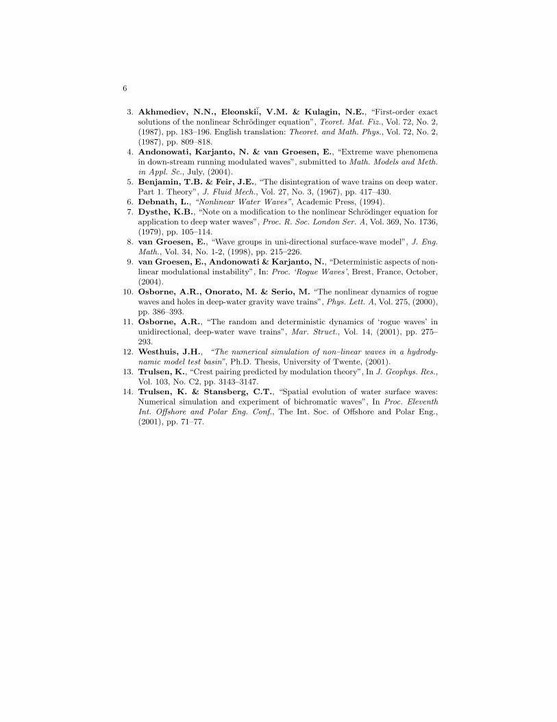
there is no wave dislocation. Furthermore, in one modulation period, there is apair of wave dislocations. Before or after this dislocation, the real-valued ampli-tude reaches its maximum value. Figure 1 shows the density plot of a physicalwave packet profile η(x, t). The wave dislocation is also visible in this figure.Figure 2 shows the evolution of the SFB from a modulated wave signal until itreaches the extreme position. We can see also in this figure that the amplitude|ψ| vanishes at some moments for the extremal position x = 0, causing phasesingularity.

The phase singularity is a well known phenomenon in physical optics. Inthe context of water waves, similar observations can be made, and also wavedislocations occur. Trulsen [13] calls it as crest pairing and crest splitting andhe explains this phenomenon as a consequence of linear dispersion.

Maximum temporal amplitude

The maximum temporal amplitude (MTA) is a useful concept to understandlong-time behavior of wave elevation. For wave propagation in the laboratory,it also gives a direct view of the consequences of an initial wave signal on thecorresponding extreme-wave signal. It is defined as

µ(x) = maxt η(x, t), (13)

5

where η(x, t) is the surface elevation as a function of space x and time t. Itdescribes the largest wave elevation that can appear at a certain position. Forlaboratory wave generation, it describes the boundary between the wet and dryparts of the wall of the basin after a long time of wave evolution.

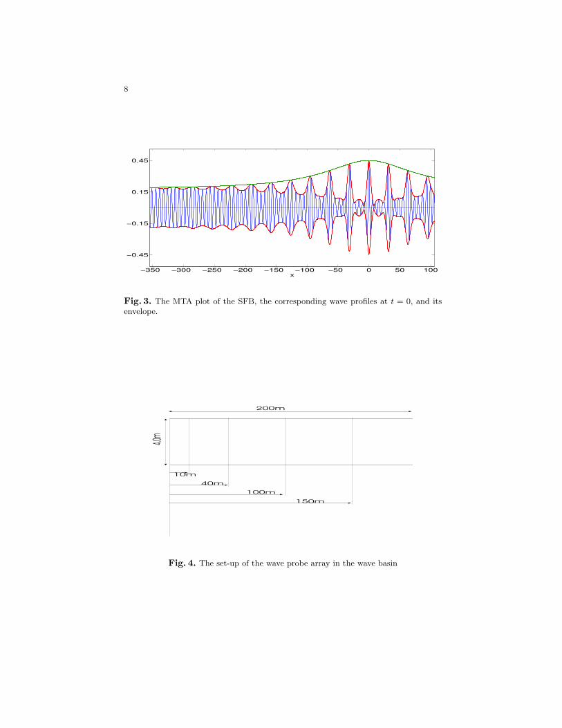
Figure 3 shows the MTA plot of the SFB in the laboratory coordinates. In thisexample, the mean water depth is 3.55 m and the wavelength is approximately6.2 m. The wave signal is generated at the left side, for example at xlab = −350m, and it propagates to the right and reaches its extremal condition at xlab = 0.A slightly modulated wave train increases in amplitude as the SFB waves travelsin the positive x-direction. Furthermore, in this example a SFB wave signal withinitial amplitude around 0.19 m can reach an extreme amplitude of 0.45 m, anamplification factor of around 2.4. After reaching its maximum amplitude, theMTA decreases monotonically and returns to its initial value.

Experimental Result

For the validation of the proposed method we performed experiments in one ofthe wave basins of marin. The basin dimensions amounted to L × B × D as200 m × 4.0 m × 3.55 m. In the basin an array of wave probes were mounted asindicated in the set–up in figure (4). The predefined wave board control signalwas put onto the hydraulic wave generator. The stroke of the wave flap wasmeasured. Main characteristics of the model test experiments:Carrier wave period is 1.685 sec. maximum wave height to be achieved (MTA)varies from 0.213m to 0.2485mAs a explanation the results for the tests with an MTA of 0.2485 will be shown,see figure( 5) to figure(7).

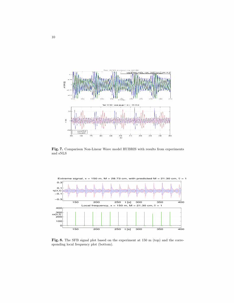
Figure 8 shows the SFB signal based on the experiment at distance 150 mfrom the wave maker, where it is expected that the signal to be extreme. Thatfigure also shows the phase singularity phenomenon when the local frequencybecomes unbounded when the real-valued amplitude vanishes or almost vanishes.The experiment result shows asymmetric form of the extreme signal while thetheoretical result of the SFB preserve the symmetry of the signal. It is suspectedthat if the modified NLS equation of Dysthe [7] is used as the governing equationfor the wave signal evolution, then there are good comparisons with experimentalmeasurements. The good comparisons are observed for the case of bi-chromaticwaves, where the modified NLS equation predicts both the evolution of individualwave crests and the modulation of the envelope over longer fetch [14].

References

1. Akhmediev, N.N. & Ankiewicz, A. “Solitons, Nonlinear Pulses and Beams”,

Optical and Quantum Electronic Ser., Vol. 5, Chapman & Hall, 1st edition, (1997).2. Akhmediev, N.N. & Korneev, V.I. “Modulation instability and periodic so-

lutions of the nonlinear Schrodinger equation”, Theor. and Math. Phys. Vol. 69,(1986), pp. 1089–1092.

6

3. Akhmediev, N.N., Eleonskii, V.M. & Kulagin, N.E., “First-order exactsolutions of the nonlinear Schrodinger equation”, Teoret. Mat. Fiz., Vol. 72, No. 2,(1987), pp. 183–196. English translation: Theoret. and Math. Phys., Vol. 72, No. 2,(1987), pp. 809–818.

4. Andonowati, Karjanto, N. & van Groesen, E., “Extreme wave phenomenain down-stream running modulated waves”, submitted to Math. Models and Meth.in Appl. Sc., July, (2004).

5. Benjamin, T.B. & Feir, J.E., “The disintegration of wave trains on deep water.Part 1. Theory”, J. Fluid Mech., Vol. 27, No. 3, (1967), pp. 417–430.

6. Debnath, L., “Nonlinear Water Waves”, Academic Press, (1994).7. Dysthe, K.B., “Note on a modification to the nonlinear Schrodinger equation for

application to deep water waves”, Proc. R. Soc. London Ser. A, Vol. 369, No. 1736,(1979), pp. 105–114.

8. van Groesen, E., “Wave groups in uni-directional surface-wave model”, J. Eng.Math., Vol. 34, No. 1-2, (1998), pp. 215–226.

9. van Groesen, E., Andonowati & Karjanto, N., “Deterministic aspects of non-linear modulational instability”, In: Proc. ‘Rogue Waves’, Brest, France, October,(2004).

10. Osborne, A.R., Onorato, M. & Serio, M. “The nonlinear dynamics of roguewaves and holes in deep-water gravity wave trains”, Phys. Lett. A, Vol. 275, (2000),pp. 386–393.

11. Osborne, A.R., “The random and deterministic dynamics of ‘rogue waves’ inunidirectional, deep-water wave trains”, Mar. Struct., Vol. 14, (2001), pp. 275–293.

12. Westhuis, J.H., “The numerical simulation of non–linear waves in a hydrody-namic model test basin”, Ph.D. Thesis, University of Twente, (2001).

13. Trulsen, K., “Crest pairing predicted by modulation theory”, In J. Geophys. Res.,Vol. 103, No. C2, pp. 3143–3147.

14. Trulsen, K. & Stansberg, C.T., “Spatial evolution of water surface waves:Numerical simulation and experiment of bichromatic waves”, In Proc. EleventhInt. Offshore and Polar Eng. Conf., The Int. Soc. of Offshore and Polar Eng.,(2001), pp. 71–77.

7

−30 −10 10 30

Fig. 2. The evolution of the SFB for ν1 = 1 from a modulated continuous wave signalinto the extreme position. From top to bottom, the signals are taken at x = −200,x = −100, x = −50, x = −30, and x = 0.

8

−350 −300 −250 −200 −150 −100 −50 0 50 100

−0.45

−0.15

0.15

0.45

x

Fig. 3. The MTA plot of the SFB, the corresponding wave profiles at t = 0, and itsenvelope.

10m

40m

100m

150m

200m

4.0m

Fig. 4. The set-up of the wave probe array in the wave basin

9

Fig. 5. Comparison Non-Linear Wave model HUBRIS with results from experimentsand sNLS

Fig. 6. Comparison Non-Linear Wave model HUBRIS with results from experimentsand sNLS

10

Fig. 7. Comparison Non-Linear Wave model HUBRIS with results from experimentsand sNLS

150 200 250 300 350 400−0.3

−0.1

0.1

0.3

t [s]

η(x,t)

Extreme signal, x = 150 m, M = 28.73 cm, with predicted M = 21.30 cm, ν~ = 1

150 200 250 300 350 400

0

100

200

300

400

t [s]

ω(x,t)

Local frequency, x = 150 m, M = 21.30 cm, ν~ = 1

Fig. 8. The SFB signal plot based on the experiment at 150 m (top) and the corre-sponding local frequency plot (bottom).