Expert Systems with Applications 41 (2014) 6876–6889

Contents lists available at ScienceDirect

Expert Systems with Applications

journal homepage: www.elsevier .com/locate /eswa

A unified hyper-heuristic framework for solving bin packing problems

http://dx.doi.org/10.1016/j.eswa.2014.04.0430957-4174/� 2014 Elsevier Ltd. All rights reserved.

⇑ Corresponding author. Tel.: +52 8181582045.E-mail addresses: eunice.lopez@itesm.mx (E. López-Camacho), terashima@

itesm.mx (H. Terashima-Marin), P.Ross@napier.ac.uk (P. Ross), gabriela.ochoa@cs.stir.ac.uk (G. Ochoa).

Eunice López-Camacho a, Hugo Terashima-Marin a,⇑, Peter Ross b, Gabriela Ochoa c

a Tecnológico de Monterrey, Av. E. Garza Sada 2501, Monterrey, NL 64849, Mexicob School of Computing, Edinburgh Napier University, Edinburgh EH10 5DT, UKc Computing Science and Mathematics, University of Stirling, Scotland, UK

a r t i c l e i n f o a b s t r a c t

Article history:Available online 10 May 2014

Keywords:Bin packing problemsEvolutionary computationHyper-heuristicsHeuristicsOptimization

One- and two-dimensional packing and cutting problems occur in many commercial contexts, and it isoften important to be able to get good-quality solutions quickly. Fairly simple deterministic heuristicsare often used for this purpose, but such heuristics typically find excellent solutions for some problemsand only mediocre ones for others. Trying several different heuristics on a problem adds to the cost. Thispaper describes a hyper-heuristic methodology that can generate a fast, deterministic algorithm capableof producing results comparable to that of using the best problem-specific heuristic, and sometimes evenbetter, but without the cost of trying all the heuristics. The generated algorithm handles both one- andtwo-dimensional problems, including two-dimensional problems that involve irregular concave poly-gons. The approach is validated using a large set of 1417 such problems, including a new benchmarkset of 480 problems that include concave polygons.

� 2014 Elsevier Ltd. All rights reserved.

1. Introduction

Finding an arrangement of pieces to cut or pack inside largerobjects is known as the cutting and packing problem. Besides theacademic interest in this NP-hard problem, there are numerousindustrial applications of its many variants. The one-dimensional(1D) and two-dimensional (2D) bin packing problems (BPPs) areparticular cases of the cutting and packing problem. The 1D BPPcan be applied, for example, to the assignment of commercialbreaks on television and for copying a collection of files to disks(Bhatia, Hazra, & Basu, 2009). For the 2D BPP, the case of rectangu-lar pieces is the most widely studied. However, the irregular case isseen in a number of industries where parts with irregular shapesare cut from rectangular materials. For instance, in the shipbuild-ing industry, plate parts with free-form shapes for use in the innerframeworks of ships are cut from rectangular steel plates, and inthe garment industry, parts of clothes and shoes are cut from fabricor leather (Okano, 2002). Other applications include the optimiza-tion of layouts within the wood, sheet metal, plastics, and glassindustries (Burke, Hellier, Kendall, & Whitwell, 2006). In theseindustries, improvements of the arrangement can result in a largesaving of material (Hu-yao & Yuan-jun, 2006).

Hyper-heuristics aim at automating the design of heuristicmethods to solve difficult search problems and providing a moregeneral procedure for optimization (Burke et al., 2003; Pillay,2012; Burke, Gendreau, Hyde, Kendall, & Ochoa, 2013). Hyper-heuristics differ from the widely-used term meta-heuristic: insteadof searching within the space of solutions, they explore the space ofheuristics (Vázquez-Rodríguez, Petrovic, & Salhi, 2007; Pappa et al.,2013). The idea is to use a variety of methods to discoveralgorithms, based on single heuristics, that have good worst-caseperformance across a range of problems and are fast in execution(Ross, 2014). There are two main types of hyper-heuristic: selec-tion hyper-heuristics, which are methods for choosing or selectingexisting heuristics, and generation hyper-heuristics which focus ongenerating new heuristics from components of existing heuristics(Burke et al., 2013; Burke et al., 2010a). The approach presentedin this paper is of the first type.

Over the last few years, one trend in combinatorial optimizationhas been to find more general solvers capable of extending to othertypes of problems within a domain and even crossing domainboundaries. For example, Burke et al. (2010b) conducted an empir-ical study that ran the same hyper-heuristic strategy in three dif-ferent domains: 1D bin packing, permutation flow shop andpersonnel scheduling. Burke, Hyde, Kendall, and Woodward(2012) presented a genetic programming system to automaticallygenerate a good quality heuristic for each instance of the one-,two-, and three-dimensional knapsack and bin packing problemswith rectilinear pieces; however, because the generated heuristics

E. López-Camacho et al. / Expert Systems with Applications 41 (2014) 6876–6889 6877

are instance-specific, the computational costs involved are non-trivial. Ochoa et al. (2012) proposed a software framework namedHyFlex (Hyper-heuristic Flexible framework) for developing cross-domain search methodologies along six different optimizationproblems.

In this paper, we introduce an evolutionary hyper-heuristicframework for solving 1D and 2D BPPs (rectangular, convex andconcave shapes) that automatically chooses which heuristic toapply at each step in building a good solution. The approachdescribed in this paper is a development of earlier work on solvingthe 1D BPP (Ross, Marín-Blázquez, Schulenburg, & Hart, 2003), the2D regular packing problem (Terashima-Marín, Farías-Zárate, Ross,& Valenzuela-Rendón, 2006) and the 2D irregular (convex only)packing problem (Terashima-Marín, Ross, Farías-Zárate, López-Camacho, & Valenzuela-Rendón, 2010). In that earlier work, thesolution construction process used an ad-hoc simplification ofthe current problem state when deciding what to do next and, inthe 2D cases, a large set of possible basic heuristics.

The main contributions of this paper are:

� A unified framework that handles 1D, 2D regular (rectangles),and 2D irregular (convex and non-convex polygons) packingproblems, together with an empirical analysis of its perfor-mance on a large unseen set of such problems.� An experiment-based methodology for deciding which heuris-

tics should be included in the framework.� A data-mining methodology for choosing the problem-state

representation to be used.� The creation of a new, large benchmark set of 2D problems that

include some non-convex polygons.

2. Background and related work

Many heuristics have been developed for specific problems butnone of them seems able to provide good-quality results for allinstances. Certain problems may contain features that enable aparticular heuristic to work well, but those features may not bepresent in other problems and so might lower that heuristic’s per-formance. Research in hyper-heuristics has developed algorithmswith some claims to more generality, but there is interest in seeingwhether even more general architectures can be developed, thatare capable of solving many different kinds of problem efficiently.Recent work by Ochoa et al. (2012), introduced a software frame-work called HyFlex for the development of cross-domain searchmethodologies. The framework provides a common interface fortreating different combinatorial problems and provides the prob-lem-specific algorithm components. Hyflex can be seen as a bench-mark framework for developing, testing and comparing thegenerality of algorithms such as selection hyper-heuristics. HyFlexhas served to test algorithms in different domains like maximumsatisfiability, one dimensional bin packing, permutation flow shop,personnel scheduling, traveling salesman and vehicle routing.Other interesting investigations have been motivated by theHyFlex system, see for example the work by Burke et al. (2010b)where several hyper-heuristics combining two heuristic selectionand three acceptance approaches were compared, and other exten-sions are given in Burke, Gendreau, Ochoa, and Walker (2011). In arelated study, Burke et al. (2012) proposed a general packing meth-odology that includes 1D, 2D (orthogonal) and 3D (orthogonal) binpacking and knapsack packing. They presented a genetic program-ming system to automatically generate a good quality heuristic foreach instance among the different problems considered althoughat a non-trivial cost per instance. HyFlex has also served as aframework for the CHeSC 2011 algorithm competition, won byMisir, Verbeeck, Causmaecker, and Berghe (2011) with an algo-rithm which provides an intelligent way of selecting heuristics,

pairing heuristics and adapting the parameters of heuristics online.They later extended this (Misir, Verbeeck, Causmaecker, & Berghe,2013) by focusing on the single heuristic sets involved and on thedistinct experimental limits. Other recent research in selectionhyper-heuristics was introduced by Kalender, Kheiri, Özcan, andBurke (2013) in which a simulated annealing-based moveacceptance method is combined with a learning heuristic selectionalgorithm to manage the single heuristics.

HyFlex and related systems use a selection hyper-heuristicapproach which operates on complete candidate solutions, per-turbing them to try to improve their quality. As such, solving aninstance typically involves some search, although usually limited.The work presented in this paper instead uses a selection hyper-heuristic approach that constructs a solution incrementally, eachstep of which could be expressed as a simple lookup of what todo next. The approach uses significant search effort to create suchan incremental solution-builder, but the amortized cost of generat-ing solutions to unseen problems is then much lower than forHyFlex-type methods. This framework has also been used for solv-ing Constraint Satisfaction Problems (Terashima-Marín, Ortiz-Bayliss, Ross, & Valenzuela-Rendón, 2008).

One of the possible limitations of this approach, as stated bySim and Hart (2013), is that if the nature of the unseen problemschanges over time, the system may need periodic re-training.

Other heuristic-selection mechanisms have been used, forexample Cowling, Kendall, and Soubeiga (2000) used a choice func-tion based on the performance of single and pairs of heuristics.Burke, Petrovic, and Qu (2006) employed a case-based reasoningapproach to tackle timetabling problems, while Bai, Blazewicz,Burke, Kendall, and McCollum (2012) proposed a learningapproach by updating the heuristic selection weights dependingon the heuristic performance after each learning period. Walker,Ochoa, Gendreau, and Burke (2012) used HyFlex to tackle a largeset of instances within the domain of Vehicle Routing Problemby using two adaptive variants of a multiple neighborhood iteratedlocal search algorithm.

3. The bin packing problem

The cutting and packing problem has been studied since 1939(Kantorovich, 1960), even though a more intensive research startedafter the middle of the twentieth century. In 2007, Wäscher,Hausner, and Schumann (2007) suggested a complete problemtypology which is an extension of Dychoff (1990). In that work,authors state that, in general terms, cutting and packing have acommon identical structure given by a set of large objects thatare to be filled and a set of items with which to do the filling, with-out overlapping other items or the edges of the objects.

In this paper, we consider the following problem types inWäscher et al. typology: (a) the 1D single bin size bin packingproblem, (b) the 2D regular single bin size bin packing problemas well as (c) the 2D irregular single bin size bin packing problem.

In the 1D BPP, there is an unlimited supply of bins, each withcapacity c > 0, and a set of n items (each one of size si < c) is tobe packed into the bins. The aim is to minimize the total numberof bins used. In the 2D BPP, there is a set L ¼ ða1; a2; . . . ; anÞ ofpieces to pack and an infinite set of identical rectangular objectsinto which the pieces are to be packed. The aim is to minimisethe number of objects needed. A problem instance I ¼ ðL; x0; y0Þ con-sists of a list of elements L and object dimensions x0 and y0. Theterm ‘2D regular BPP’ is mainly used when all pieces are rectangu-lar and the term ‘2D irregular BPP’ refers to the case where piecescan be polygonal, not just rectangular. We deal only with the off-line BPP, in which the list of pieces to be packed is given inadvance.

6878 E. López-Camacho et al. / Expert Systems with Applications 41 (2014) 6876–6889

There are very few studies available of the 2D irregular BPP,despite its practical importance. Ponce-Pérez, Pérez-García, andAyala-Ramírez (2005) proposed a genetic algorithm basedapproach and tested it on one four-piece instance. Okano (2002)solved three real instances from a problem more general thanour 2D irregular single bin size BPP, using variable bin sizes, wherethe solution involves finding appropriate sizes of material objects(bins) among given standard sizes in order to reduce waste. Babuand Babu (2001) presented the solution for one instance in whichthe objects are all of different size and shapes.

For all non-trivial BPP problems, exhaustive search is impracti-cal and heuristic methods are needed. For the 2D BPP, heuristicmethods typically involve iterating two actions: first, selectingboth the next piece to be placed and the corresponding object inwhich to place it; and then, placing the selected piece in a positioninside the object according to a given criterion. Some approachesmay choose to include local search in these steps. For the 1DBPP, the placement step is unnecessary. In our approach, the twoactions are done while working with partial solutions because heu-ristics construct a layout piece by piece, and feasibility is embed-ded into the heuristic since each piece is placed in a feasibleposition on the stock sheet and not moved thereafter.

Some metaheuristics for the 1D BPP have been implemented(Ducatelle & Levine, 2001; Falkenauer, 1996; Rohlfshagen &Bullinaria, 2010). For the 2D cutting and packing problem,Hopper and Turton (2001) reviewed metaheuristic implementa-tions. Hyper-heuristic search has been applied to the 1D BPP(Pillay, 2012; Ross et al., 2003; Burke, Woodward, Hyde, &Kendall, 2007; Marín-Blázquez & Schulenburg, 2006; Sim, Hart, &Paechter, 2012) and different 2D BPPs (Terashima-Marín et al.,2006; Terashima-Marín et al., 2010; Burke, Hyde, Kendall, &Woodward, 2008; Garrido & Riff, 2007).

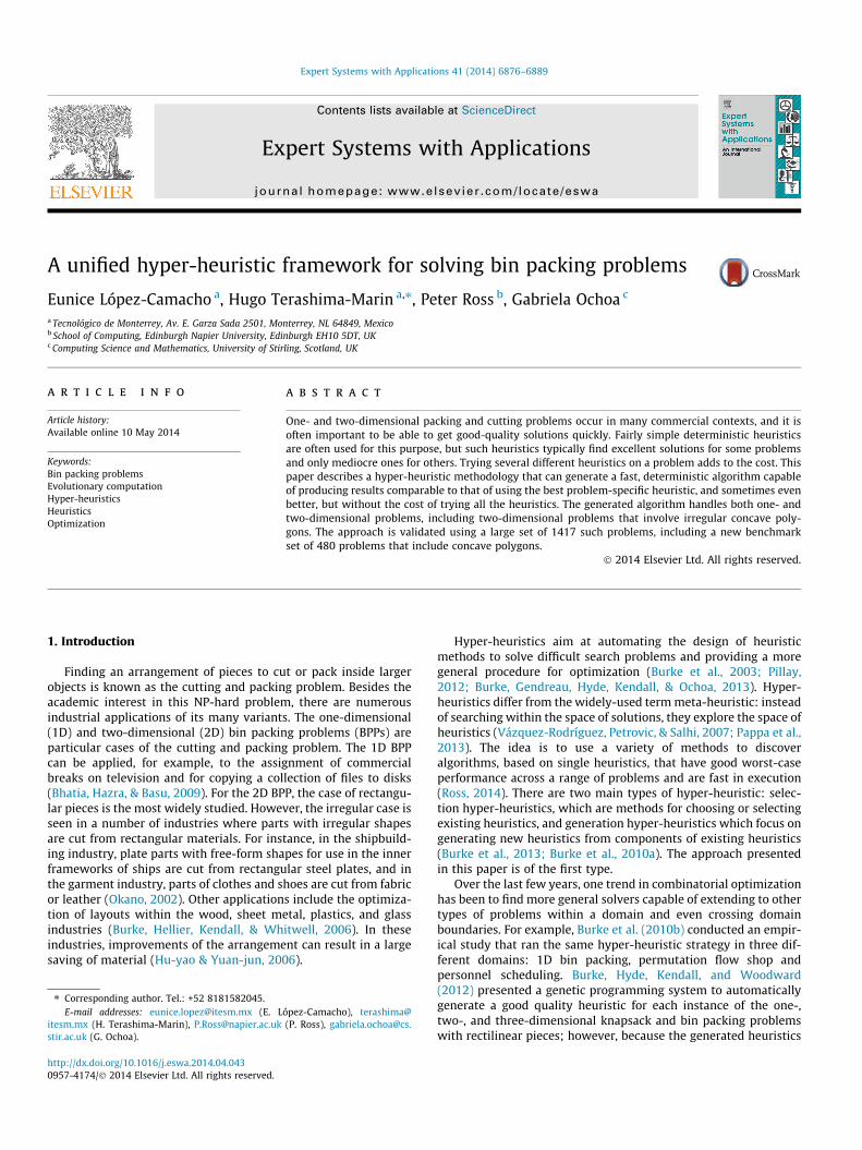
Fig. 1. Each block in a chromosome represents a point in the space of states labelledwith a single heuristic. The hyper-heuristic solves a problem instance by finding theclosest single heuristic at every solution stage.

4. The evolutionary hyper-heuristic framework

The method presented in this paper is based on a genetic algo-rithm (GA) that evolves sets of condition-action rules that specifywhat to do next in any given problem state. Each individual inthe GA population is a possible hyper-heuristic, specifying a com-plete set of such condition-action rules. This kind of GA-basedapproach has produced encouraging results in previous work(Ross et al., 2003; Terashima-Marín et al., 2006; Terashima-Marínet al., 2010).

According to the classification of hyper-heuristic approachessuggested by Burke et al. (2010a), our GA-generated hyper-heuris-tics fall into the category of selection hyper-heuristics because theyselect the single heuristics to be applied rather than generatingnew heuristics from components such as mutation and selectionoperators.

The key idea in our constructive approach is to build a completesolution by deciding what to do at each stage, including the initialstage. Here, what to do means choosing heuristics to place piecesand thus extend the solution. Each stage is described by a simpli-fied representation of the problem state. We hypothesize that iftwo states are very similar then we would want to do the samething in either state.

The hyper-heuristic has the following general form. Any state ofthe partially-solved problem is described using a fixed, simplifiednumeric representational scheme that expresses the state as apoint in a unit hypercube of some sort. The GA’s task is to find arepresentative set of points within, or close to, this hypercubeand to label each such point with a specific heuristic step. Thisset of labelled points represents the hyper-heuristic, and it is uti-lized as follows. Until a solution is completely constructed, repeat-edly: (a) encode the current problem state as a vector P; (b) find

the labelled point L that is closest to P (this could be handled bydividing the space into tiny cubes and simply doing a lookup);(c) apply the heuristic step specified by that label to extend thesolution. The question of what simplified representation to use isaddressed in Section 5.4.

The type of GA used is a so-called ‘messy’ GA (Deb & Goldberg,1991; Goldberg, Deb, & Korb, 1989), because of its variable lengthchromosomes. Each chromosome is composed of a series of blocks.Each block represents one labelled point, and consists of a vectoridentifying a point in the hypercube, and a final integer that iden-tifies a heuristic by indexing a fixed array of available heuristics. Achromosome therefore consists of a number of points in a simpli-fied state space, each point being labelled with a single heuristic,exemplifed in Fig. 1 which shows six labelled points h1 . . . h6 andthree successive problem states P; P0; P00 in an overly simplisticthree-dimensional hypercube. Clearly, not every point in such ahypercube will represent a valid state. For example, it is not verylikely that (say) the features percentage of small items and averageof items sizes would have large values at the same time.

Available problem instances are divided into separate trainingand testing sets. In the GA, chromosomes are evaluated using onlya few instances from the training set. The testing set is reserved forevaluating the performance of the end result of the evolutionaryprocess.

4.1. The fitness function

Each hyper-heuristic (chromosome) and each individual heuris-tic can be evaluated on any given problem in the same way:

Q ¼PN

i¼1U2i

Nð1Þ

where N is the total number of objects used and Ui is the fractionalspace utilization for each object i, so, 0 6 Ui 6 1. We seek to maxi-mize Q. A simple application of Lagrange multipliers shows that Q isminimized when all the Ui are equal (empty space is shared outequally), and because Q is concave upwards, simple geometric con-siderations show that Q is maximized at some boundary point whenas many Ui as possible are as large as possible. Now, let QkðHÞ be theperformance of algorithm H on problem k, as defined in (1); if thefixed heuristics are F1; F2; . . . F6 then define Bk to be the Fi that max-imizes QkðFiÞ, i.e. the fixed heuristic that gives the best performanceon problem k.

E. López-Camacho et al. / Expert Systems with Applications 41 (2014) 6876–6889 6879

Each chromosome is evaluated on some number m of problemsand its fitness is computed as the average difference between thesolution quality obtained by the chromosome with respect to theresult given by the best single heuristic for every particularinstance:

f ðHHÞ ¼Pm

k¼1ðQ kðHHÞ � Q kðBkÞÞm

ð2Þ

Note that f ðHHÞ could be negative if the hyper-heuristic averageperformance is below the performance of the best heuristic foreach instance solved. We expect that the evolutionary processfinds a chromosome with positive value of f ðHHÞ.

4.2. The GA cycle

The evolutionary process is given by the following steps:

1. Generate the initial population. Each individual is comprised of10 to 15 blocks.

2. Randomly assign m ¼ 5 problems from the training set to eachchromosome and compute the chromosome fitness based onthose problems (Eq. (2)).

3. Apply selection with tournament of size 2, crossover and muta-tion operators to produce two children.

4. Randomly assign m ¼ 5 problems to each new child and esti-mate its fitness.

5. Replace the two worst individuals with the new offspring pro-vided they are of better fitness.

6. Assign one additional and new problem to every individual inthe new population and update fitness. Now the fitness on eachindividual is based on the number of instances it has seen sofar; at age T P 0, a chromosome’s evaluation is based on a totalof m ¼ 5þ T problems.

7. Repeat from Step 3 until a termination criterion is reached.

If the GA is run with a small population of size P, this means anychromsome is unlikely to be assessed on very much more thanabout 5þ P=2 problems. However, the chromosome’s ancestorswill have collectively seen very many more than this.

The GA uses two crossover and three mutation operators. Theseoperators were taken from the previous implementation of thesolution model for the 1D BPP (Ross et al., 2003) and the 2D regularBPP (Terashima-Marín et al., 2006; Terashima-Marín et al., 2010).The probability for applying each type of crossover or mutationoperator was suggested by some early testing in the investigationfor the 1D case (Ross et al., 2003).

Both of the following crossover operators employed have thesame probability of being chosen. The one-point crossover oper-ator works at block level, and exchanges 10% of blocks betweenparents, meaning that the first child obtains 90% of informationfrom the first parent, and 10% from the second one, and viceversa. This operator shuffles blocks, so the blocks passed froma parent to an offspring are not in consecutive order; that is,gene linkage is broken. The two-point crossover operator is verysimilar to the normal two-point crossover. For each individual,we first select two blocks and then a point inside each blockis chosen. Since the number of blocks in each chromosome isvariable, the cut points in each parent are independently cho-sen. However, the points selected inside each correspondingblock are forced to be the same for both parents, to avoidchanging the meaning of any numbers, so that the recombina-tion produces an exact number of blocks. The blocks and pointsare chosen using a uniform distribution. If one parent has alength of up to two blocks, then the individual is completelyremoved and recreated randomly with a number of blocks from10 to 15. The other selected individual for crossover is copied

exactly. The idea is to penalize chromosomes with a very smallnumber of blocks.

Three mutation operators are used: add-block, remove-block,and in-block. Mutation is applied with probability 0.1, and thespecific operator is randomly selected from along these threechoices: in-block is twice as likely to be selected as the othertwo. The add-block mutation operator randomly generates anew block and adds it at the end of the chromosome, unlessthe length is 20 or more in which case a random block is deletedinstead. The remove-block mutation operator randomly selectsand eliminates a block within the chromosome unless the lengthis 6 blocks or less, in which case it adds a new one. The in-blockoperator randomly selects a position inside a random block andmutates it. If the selected position is a heuristic specifier, a ran-dom one is chosen. If it is a hypercube co-ordinate, a new valueis chosen from an Nð0:5;0:5Þ distribution and truncated to lie inthe range �2 to 3.

Experiments in this investigation were carried out using a pop-ulation size of 30, crossover probability of 1.0, mutation probabilityof 0.10, and 80 generations. These parameters worked well in pre-liminary experimentation and were used in previous studies(Terashima-Marín et al., 2010).

5. Implementation methodology

This section describes the implementation details includinghow the set of single heuristics and instances was gathered andthe process for getting an adequate problem-state representationscheme.

5.1. Set of heuristics used

The following six heuristic approaches were employed. Heuris-tics are criteria to select the next piece to be placed and the corre-sponding object to place it. The 1D and 2D cases of the BPP sharethe same selection heuristics. For the 2D BPP, a placement heuristicwas additionally used.

1. First Fit Decreasing (FFD). Considers the open objects in the orderthey were opened and places the largest piece in the first objectwhere it fits. If the piece does not fit into any open object, FFDopens a new object to pack the piece.

2. Filler. Sorts the unplaced pieces in decreasing order of size andplaces as many pieces as possible within the open objects. If nosingle piece could be placed, it opens a new object and places asmany pieces as possible in it.

3. Best Fit Decreasing (BFD). Sorts the unplaced pieces in decreasingorder of size and places the next piece in the open object whereit best fits, that is, in the object that leaves minimum waste. Ifthe piece does not fit into any open object, BFD opens a newobject to pack the piece.

4. Djang and Finch with initial fullness of 1/4 (DJD1/4). Places items inan object, taking items by decreasing size, until the object is atleast one-fourth full. Then, it initializes w ¼ 0, a variable indi-cating the allowed waste, and looks for combinations of one,two, or three items producing a waste w or less. If any combina-tion fails, it increases w by one twentieth of the object. When wreaches the amount of free space of the object, a new object isopened.

5. Djang and Finch with initial fullness of 1/3 (DJD1/3). Same asDJD1/4, once the object is full up to 1/3 it tries combinationsof pieces.

6. Djang and Finch with initial fullness of 1/2 (DJD1/2). Same asDJD1/4, once the object is full up to 1/2 it tries combinationsof pieces.

6880 E. López-Camacho et al. / Expert Systems with Applications 41 (2014) 6876–6889

All of these are one-step constructive heuristics for the offlineBPP. These approaches can often produce reasonable quality solu-tions with little computational cost (Bennell & Oliveira, 2009).DJD1/4, DJD1/3 and DJD1/2 are variations of the DJD heuristic(López-Camacho, Ochoa, Terashima-Marín, & Burke, 2013). In pre-liminary experimentations, it has been found that DJD1/4, DJD1/3

and DJD1/2, though similar, present a different behavior in differenttypes of problem instances. For example, 2D instances with hugepieces are generally better solved by DJD1/4; while DJD1/3 is betterwith instances with small pieces (averaging below 1/10 of theobject area). These heuristics were selected from a larger set,because they produced the best single-heuristic results in a preli-minary study.

For 2D problems, the heuristic called Constructive Approachwith Maximum Adjacency (CAD) was employed for finding theactual placement of the selected piece in a valid position insidethe object. This heuristic is partially based on the approach sug-gested by Uday, Goodman, and Debnath (2001) and adapted byTerashima-Marín et al. (2010). It explores several possible posi-tions and the one with the largest adjacency i.e. the commonboundary between its perimeter and the placed pieces and theobject edges is selected as the position of the new piece. In caseof tie, the most bottom-left position is chosen. This heuristic waschosen because of its good performance in López-Camacho et al.(2013). There are several approaches to handle the geometry ofirregular shapes, such as the nofit polygon or the phi function(Bennell & Oliveira, 2009; Alvarez-Valdes, Martinez, & Tamarit,2013; Bennell, Scheithauer, Stoyan, & Romanova, 2010). Inparticular, our implementation is based on trigonometry(López-Camacho et al., 2013).

Previous studies had included in their heuristic repository everypossible combination of several selection and placement heuristicsconsidered, without performing any quality filter. Therefore, a verylong list of heuristics comprised the heuristic repository(Terashima-Marín et al., 2006; Terashima-Marín et al., 2010). Asa consequence, after the hyper-heuristics were built, most of thesingle heuristics were not called when solving a large set ofinstances. We conjecture that the presence of poor-quality heuris-tics delays the evolutionary process because it starts with an initialpopulation with many unnecessary poor-quality hyper-heuristicsand it takes time to weed them out.

Table 1Description of problem instances.

1D Convex 2D

Type Num. of instances Num. of pieces Type Num. of instanc

DB1 n1 45 50 Conv A 30DB1 n2 45 100 Conv B 30DB1 n3 45 200 Conv C 30DB1 n4 45 500 Conv D 30DB2 n1 30 50 Conv E 30DB2 n2 30 100 Conv F 30DB2 n3 30 200 Conv G 30DB2 n4 30 500 Conv H 30Wäscher 17 57–239 Conv I 30Trip60 20 60 Conv J 30Trip120 20 120 Conv K 30Trip249 20 249 Conv L 30Trip501 20 501 Conv M 30

Conv N 30Conv O 30Conv P 30Conv Q 30Conv R 30

Total 397 Total 540

5.2. Testbed instances

Our experimental testbed is comprised of a total of 1417instances which are summarized in Table 1.

The 397 one-dimensional problem instances are from the liter-ature. The first eight types of 1D instances in Table 1 are fromScholl, Klein, and Jürgens (1997), where we chose one out of everyfour instances in Scholl’s data bases 1 and 2. Next instances comefrom Wäscher and Gau (1996) and the last four types of 1Dinstances are triplets from Falkenauer (1996) whose optimal solu-tions have exactly 3 items per bin with zero waste. These instancesthat are triplets originally had item sizes rounded to one decimalplace. They were scaled up by a factor of 10 so that all values arenow integers.

We have 540 two-dimensional instances with only convexpolygonal pieces that were randomly generated by Terashima-Marín et al. (2010). This testbed also includes 30 rectangularinstances (type Conv I). All the 2D convex instances, except typeConv G, have an optimum with zero waste; therefore, in the opti-mum solution, all objects must be filled up to 100%.

The 480 new 2D instances containing some non-convex poly-gons were randomly produced for this study. Of these, 240 weregenerated splitting at least five pieces from each instance fromtypes Conv A, Conv B, Conv C, Conv F, Conv H, Conv L, Conv M andConv O, respectively. Convex pieces from these instances were ran-domly selected and split into two pieces: one convex and one non-convex. The other 240 of the non-convex instances were producedby creating new convex instances and then splitting some of thepieces into non-convex polygons. Types NConv U, NConv W andNConv X were produced by splitting some pieces from instancesthat already had non-convex pieces. The 2D irregular instance setused in this study can be found at http://paginas.fe.up.pt/�esi-cup/tiki-index.php.

There is a variety of instance feature values in our experimentaltestbed. For example, there are instances whose pieces have anaverage size of 1/30 of the object, while other instances have hugepieces (averaging almost 2/3 of object size). Either the optimumnumber of objects or the best-known result ranges between 2and 273. In the 2D problems, rectangularity (the ratio of the areaof a piece to the area of the smallest enclosing rectangle) variesbetween 0.35 and 1.

Non Convex 2D

es Num. of pieces Type Num. of instances Num. of pieces

30 NConv A 30 35–5030 NConv B 30 40–5236 NConv C 30 42–6060 NConv F 30 35–4560 NConv H 30 42–6030 NConv L 30 35–4536 NConv M 30 45–5836 NConv O 30 33–4360 NConv S 30 17–2060 NConv T 30 30–4054 NConv U 30 20–3330 NConv V 30 15–1840 NConv W 30 24–2860 NConv X 30 25–3928 NConv Y 30 40–5056 NConv Z 30 606054

Total 480

Fig. 2. One convex and one non-convex polygon created by the developedalgorithm.

Table 2Cluster membership for the 1D and 2D instances. According to fitness of the six singleheuristics considered.

Cluster 1D Convex 2D Non convex 2D Total

C1 224 209 287 720C2 14 58 48 120C3 4 29 36 69C4 85 43 41 169C5 69 103 81 253C6 1 17 18C7 19 15 34C8 19 15 34

Total 397 480 540 1417

E. López-Camacho et al. / Expert Systems with Applications 41 (2014) 6876–6889 6881

5.3. Algorithm for producing random instances with non-convex pieces

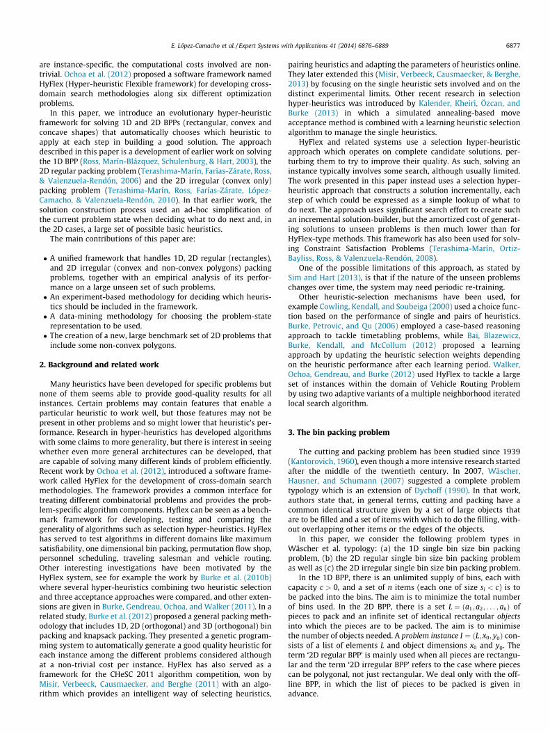
The process for creating problems with non-convex piecesstarts with a set of convex pieces, each of which is defined by aset of corners that have integer co-ordinates. Then, a selected con-vex piece can be split into two pieces, one convex and other con-cave, by (a) selecting two edges; (b) for each of these two edges,either choosing an integer-valued interior point or (if none exist)choosing one of the endpoints of the edge, thus obtaining twopoints Q and R on the border of the piece; (c) choosing an inte-ger-valued interior point P, and joining Q to P to R and then split-ting the piece into two, one of them being concave (see Fig. 2).

Finally, the algorithm randomizes the order of all the pieces sothat the two parts of a split piece are very unlikely to be adjacent inthe list of pieces.

When this algorithm is applied to an instance that already hasnon-convex shapes it is possible to produce U-shaped polygonsor even shapes with an internal empty space reached by a smallerentrance (resembling letter G). Shapes with holes are not producedby the algorithm.

5.4. Developing a problem-state representation for the testbedinstances

We need to summarize each instance state by a numerical vec-tor that quantifies some of its relevant features. Thus, the aim is tofind a feature set that correlates fairly well with performance of thesix heuristics. A great deal of the performance of a selection hyper-heuristic model may depend on the choice of representation of theproblem state and the choice of the particular set of heuristics used(Ross, 2014). Messelis and Causmaecker (2014) have also recentlyargued that it is crucial to find a set of instance features that cap-tures the internal structure of a problem domain and that is relatedto the performance of an algorithm. Finding such a set is not obvi-ous. We have adopted the data mining based methodology pro-posed by López-Camacho, Terashima-Marín, and Ross (2010), inorder to select the most representative features to characterizean instance of any type (1D, 2D regular, and 2D irregular).

The general methodology comprises six steps that we applied asfollows:

Step 1. Each instance is solved by each of the six single heuristicsand its performance is computed with Eq. (1).

Step 2. The performance of the six single heuristics for eachinstance is considered as a vector in R6, normalized tohave length 1. Normalization removes the distinctionbetween easy or hard instances in the measure of perfor-mance so that only the relative performance of the variousheuristics matters.

Step 3. All instances are grouped into homogeneous clustersbased on the normalized performance of the six singleheuristics. The clusters will be used in Step 6, to find those

problem-state features that are significant in predictingthe clusters. We chose the k-means clustering techniquewhich is a widely used algorithm (Arthur & Vassilvitskii,2006). In this procedure the number of clusters has to beprovided by the user, however there exist someapproaches for selecting a good number of clusters. Inour research, the number of clusters was eight and wasdetermined according to the Hartigan criteria (Chiang &Mirkin, 2007). With the number of clusters chosen, 30 ran-dom k-means initializations were run, and we decided touse the seed that produces clusters which minimize thetotal intra-cluster variance (squared error function), givenby:

Pki¼1

Pxj2Siðxj � ljÞ

2 where there are k clustersSi; i ¼ 1;2; . . . ; k, and li is the centroid or mean point ofall the points xj 2 Si. After obtaining the number ofinstances associated to each cluster, Table 2 summarizesthe cluster membership according to dimensionality andconvexity. Note that many instance types are split into dif-ferent clusters. Instances in the same cluster have similarbehavior when solved by the six heuristics consideredand we attempt to find which features these instanceshave in common.

Step 4. This step consists of finding instance features that may berelevant to the ability of the heuristics to solve eachinstance. 23 numerical features were computed for eachinstance. The last two features are devoted to measureconcaveness. The features are: (1) Number of pieces, (2)Mean number of sides for the instance pieces, (3) Varianceof the number of sides of all instance pieces, (4) Mean areafor the instance pieces (area for each piece is measured asa fraction of the object total area), (5) Variance of the areaof all instance pieces, (6) Mean height for the instancepieces (height for each piece is measured as a fraction ofthe object height with the difference between its maxi-mum and minimum y coordinates), (7) Variance of theheight of all instance pieces, (8) Mean width for theinstance pieces (width for each piece is measured as a frac-tion of the object width with the difference between itsmaximum and minimum x coordinates), (9) Variance ofthe width of all instance pieces, (10) Mean rectangularityfor the instance pieces, (11) Variance of the rectangularityof all instance pieces, (12) Mean ratio (largest side)/(small-est side) for the instance pieces, (13) Variance of the ratio(largest side)/(smallest side) of all instance pieces, (14)Percentage of large pieces (whose area is greater than1=2 of the object total area), (15) Percentage of smallpieces (whose area is less than or equal to 1=4 of the objecttotal area), (16) Percentage of right internal angles (respectto the total angles of all pieces of the instance), (17) Per-centage of vertical/horizontal sides (respect to the totalsides of all pieces of the instance), (18) Percentage of highrectangularity pieces (items which rectangularity is

6882 E. López-Camacho et al. / Expert Systems with Applications 41 (2014) 6876–6889

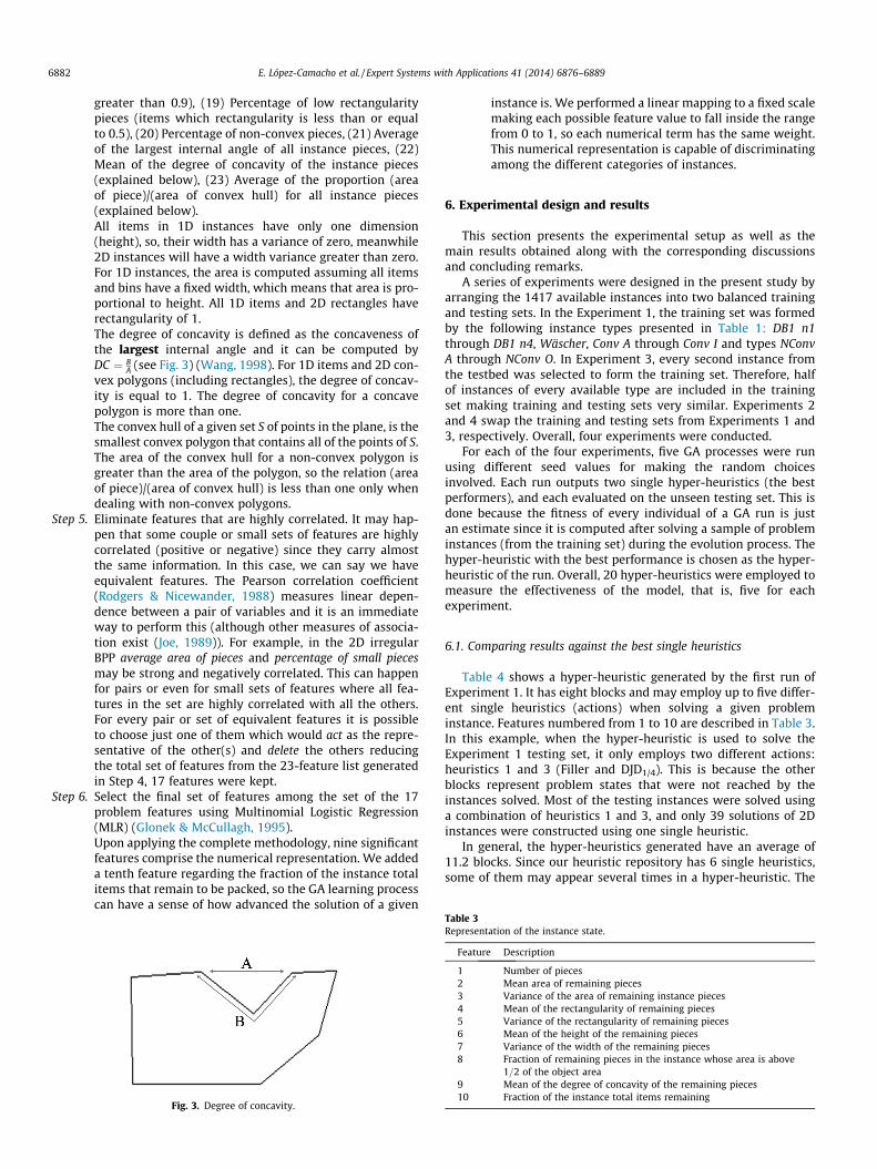
greater than 0.9), (19) Percentage of low rectangularitypieces (items which rectangularity is less than or equalto 0.5), (20) Percentage of non-convex pieces, (21) Averageof the largest internal angle of all instance pieces, (22)Mean of the degree of concavity of the instance pieces(explained below), (23) Average of the proportion (areaof piece)/(area of convex hull) for all instance pieces(explained below).All items in 1D instances have only one dimension(height), so, their width has a variance of zero, meanwhile2D instances will have a width variance greater than zero.For 1D instances, the area is computed assuming all itemsand bins have a fixed width, which means that area is pro-portional to height. All 1D items and 2D rectangles haverectangularity of 1.The degree of concavity is defined as the concaveness ofthe largest internal angle and it can be computed byDC ¼ B

A (see Fig. 3) (Wang, 1998). For 1D items and 2D con-vex polygons (including rectangles), the degree of concav-ity is equal to 1. The degree of concavity for a concavepolygon is more than one.The convex hull of a given set S of points in the plane, is thesmallest convex polygon that contains all of the points of S.The area of the convex hull for a non-convex polygon isgreater than the area of the polygon, so the relation (areaof piece)/(area of convex hull) is less than one only whendealing with non-convex polygons.

Step 5. Eliminate features that are highly correlated. It may hap-pen that some couple or small sets of features are highlycorrelated (positive or negative) since they carry almostthe same information. In this case, we can say we haveequivalent features. The Pearson correlation coefficient(Rodgers & Nicewander, 1988) measures linear depen-dence between a pair of variables and it is an immediateway to perform this (although other measures of associa-tion exist (Joe, 1989)). For example, in the 2D irregularBPP average area of pieces and percentage of small piecesmay be strong and negatively correlated. This can happenfor pairs or even for small sets of features where all fea-tures in the set are highly correlated with all the others.For every pair or set of equivalent features it is possibleto choose just one of them which would act as the repre-sentative of the other(s) and delete the others reducingthe total set of features from the 23-feature list generatedin Step 4, 17 features were kept.

Step 6. Select the final set of features among the set of the 17problem features using Multinomial Logistic Regression(MLR) (Glonek & McCullagh, 1995).Upon applying the complete methodology, nine significantfeatures comprise the numerical representation. We addeda tenth feature regarding the fraction of the instance totalitems that remain to be packed, so the GA learning processcan have a sense of how advanced the solution of a given

Fig. 3. Degree of concavity.

instance is. We performed a linear mapping to a fixed scalemaking each possible feature value to fall inside the rangefrom 0 to 1, so each numerical term has the same weight.This numerical representation is capable of discriminatingamong the different categories of instances.

6. Experimental design and results

This section presents the experimental setup as well as themain results obtained along with the corresponding discussionsand concluding remarks.

A series of experiments were designed in the present study byarranging the 1417 available instances into two balanced trainingand testing sets. In the Experiment 1, the training set was formedby the following instance types presented in Table 1: DB1 n1through DB1 n4, Wäscher, Conv A through Conv I and types NConvA through NConv O. In Experiment 3, every second instance fromthe testbed was selected to form the training set. Therefore, halfof instances of every available type are included in the trainingset making training and testing sets very similar. Experiments 2and 4 swap the training and testing sets from Experiments 1 and3, respectively. Overall, four experiments were conducted.

For each of the four experiments, five GA processes were runusing different seed values for making the random choicesinvolved. Each run outputs two single hyper-heuristics (the bestperformers), and each evaluated on the unseen testing set. This isdone because the fitness of every individual of a GA run is justan estimate since it is computed after solving a sample of probleminstances (from the training set) during the evolution process. Thehyper-heuristic with the best performance is chosen as the hyper-heuristic of the run. Overall, 20 hyper-heuristics were employed tomeasure the effectiveness of the model, that is, five for eachexperiment.

6.1. Comparing results against the best single heuristics

Table 4 shows a hyper-heuristic generated by the first run ofExperiment 1. It has eight blocks and may employ up to five differ-ent single heuristics (actions) when solving a given probleminstance. Features numbered from 1 to 10 are described in Table 3.In this example, when the hyper-heuristic is used to solve theExperiment 1 testing set, it only employs two different actions:heuristics 1 and 3 (Filler and DJD1/4). This is because the otherblocks represent problem states that were not reached by theinstances solved. Most of the testing instances were solved usinga combination of heuristics 1 and 3, and only 39 solutions of 2Dinstances were constructed using one single heuristic.

In general, the hyper-heuristics generated have an average of11.2 blocks. Since our heuristic repository has 6 single heuristics,some of them may appear several times in a hyper-heuristic. The

Table 3Representation of the instance state.

Feature Description

1 Number of pieces2 Mean area of remaining pieces3 Variance of the area of remaining instance pieces4 Mean of the rectangularity of remaining pieces5 Variance of the rectangularity of remaining pieces6 Mean of the height of the remaining pieces7 Variance of the width of the remaining pieces8 Fraction of remaining pieces in the instance whose area is above

1=2 of the object area9 Mean of the degree of concavity of the remaining pieces10 Fraction of the instance total items remaining

Table 4Hyper-heuristic generated in the first run of Experiment 1.

Block Feature Action

1 2 3 4 5 6 7 8 9 10

1 1.03 1.33 0.80 0.49 0.64 0.22 0.81 0.43 0.91 0.65 0 (FFD)2 �0.08 0.16 0.77 0.17 0.43 0.74 �0.34 0.37 0.92 0.30 1 (Filler)3 1.06 0.89 0.40 �0.36 0.70 0.51 �0.03 0.84 1.39 0.36 2 (BFD)4 0.34 0.91 0.56 0.27 0.41 0.93 0.87 0.82 0.91 0 2 (BFD)5 1.08 1.25 0.83 1.26 0.51 0.04 0.49 0.02 0.70 0.91 0 (FFD)6 0.57 0.10 0.46 0.52 0.67 0.39 0.87 0.44 �0.61 0.43 3 (DJD1/4)7 0.52 0.80 1.14 0.34 0.52 0.33 0.80 1.05 0.17 �0.42 4 (DJD1/3)8 0.70 1.08 0.87 �0.23 0.52 �0.59 0.89 0.23 0.55 0.31 2 (BFD)

E. López-Camacho et al. / Expert Systems with Applications 41 (2014) 6876–6889 6883

six single heuristics considered were employed by at least one ofthe hyper-heuristics generated along the experiments.

Each one of the twenty generated hyper-heuristics employed acombination of two to five single heuristics when solving the test-ing set of the corresponding experiment. Complete results areshown in Table 5. Figures in cells indicate the percentage ofinstances that employs a particular number of extra objects (leftcolumn) when compared against results provided by the best sin-gle heuristic for each instance. We present results averaging thefive best hyper-heuristics, each selected from each complete runin the experiment, as well as the results on the average of the

Table 5Number of extra objects obtained by hyper-heuristics and single heuristics when comparpercentage of cases). Zero values are displayed as blank cells.

Extra objects Hyper-heuristics Single h

Average 2B-Avg Best FFD

Experiment 16 �2 0.6 0.7�1 0.6 2.8 2.70 86.2 93.4 94.9 62.11 13.2 3.2 1.7 23.02 3.93 1.1P 4 9.9

Experiment 26 �2�10 92.6 98.2 100 70.21 7.4 1.8 21.12 6.23 2.4P 4 0.1

Experiment 36 �2 0.3�1 1.1 0.80 94.6 95.9 96.9 66.11 5.4 3.0 2.0 21.62 5.43 2.0P 4 4.9

6 �2 0.1�1 1.0 0.80 91.7 95.6 97.9 66.11 5.1 3.4 1.1 22.42 1.6 4.83 0.6 1.6P 4 1.1 5.1

All experiments6 �2 0.1 0.4�1 0.1 1.2 1.60 91.3 95.8 97.4 66.11 7.8 2.9 0.6 222 0.4 5.13 0.1 1.8P 4 0.3 5

two-best hyper-heuristics and the best hyper-heuristic per exper-iment, considering the testing instance set. In general, the averageperformance of the five hyper-heuristics produced per experimentis favorable since it clearly beats four of the single heuristics and itis very competitive against the other two, DJD1/4 and DJD1/3. Now,if we observe the performance of the two-best hyper-heuristics(average) and the best hyper-heuristics per experiment, the resultsdefinitively are better than those provided by any single heuristics.Two important aspects we can point out here: there is a saving inthe number of objects for a percentage of the instances, and thelargest number of extra objects used by them is no greater than

ed against the results of the best single heuristic for each instance (figures indicate

euristics

Filler BFD DJD1/4 DJD1/3 DJD1/2

63.0 64.5 96.1 93.0 72.022.0 20.7 3.9 6.6 14.84.1 3.8 0.4 2.81.1 1.1 0.89.9 9.9 9.6

69.4 70.6 96.3 95.8 72.821.8 20.5 3.5 4.2 19.56.2 6.4 0.1 6.12.4 2.4 1.60.1 0.1

66.1 67.2 96.0 94.1 72.221.6 20.3 3.8 5.6 17.15.4 5.5 0.1 0.3 4.82.0 2.0 1.34.9 4.9 4.7

66.3 67.8 96.3 94.6 72.622.1 20.9 3.7 5.2 17.24.9 4.7 0.1 4.11.6 1.6 1.15.1 5.1 4.9

66.2 67.5 96.2 94.4 72.421.9 20.6 3.7 5.4 17.15.2 5.1 0.1 0.2 4.41.8 1.8 1.25 5 4.8

Table 6Comparison of our approach versus Mumford’s GSA for Scholl and Faulkner instances.

Instance Number of objects

Optimum GSA Best simple heuristic Best hyper-heuristic

N4C3W2A 203 204 204 204N4C3W4A 216 217 217 217N4W1B1R0 167 167 167 167N4W3B1R0 71 71 72 73

Trip60 20 21 21 21Trip120 40 41 41 41Trip249 83 84 84.8 84.75Trip501 167 168 170.8 170.05

6884 E. López-Camacho et al. / Expert Systems with Applications 41 (2014) 6876–6889

one, usually for a small percentage of the instance set. For example,in Experiment 1 the average of the two-best and the best hyper-heuristic required one object less in 2.8% and 2.7% of instances,respectively, and two or more objects less in 0.6% and 0.7% ofinstances, respectively. For Experiment 2, the best hyper-heuristicobtains the same results that the best single heuristic 100% oftimes; which means that the hyper-heuristic learns to behave asthe best single heuristic per problem. Along all experiments, thebest hyper-heuristic delivered fewer objects than the best singleheuristic for 2% of the instances. We could state that the hyper-heuristics produced are capable of learning to perform as well asthe best single heuristic for each instance, and for some cases, evenbetter. In other words, these hyper-heuristics may be considered asgeneral solving methods.

It has been confirmed that solving an instance with a hyper-heuristic is faster than solving it with each of the single heuristicsand then choosing the best result (Terashima-Marín et al., 2010).We ran the algorithms on a 1.66 GHz PC with 1.98 GB of RAM. Oncethe hyper-heuristic is generated, it solves each instance in 20 s onaverage.

For most cases, the best hyper-heuristic achieves the samenumber of objects than the best single heuristic (higher percent-ages in Table 5 are in the 0-object row). We ran the non-parametricMann–Whitney statistical test for means comparison of extraobjects between 1D and 2D cases. We want to know if thehyper-heuristic model performance is different for 1D and 2Dinstances. For Experiment 1, the extra number of objects deliveredby the best hyper-heuristic is statistically different for 1D and for2D instances (p-value ¼ 0:001). For the rest of the experiments,the difference is not significant between 1D and 2D BPP. Whenwe perform a comparison of means test between results for convexand non-convex 2D instances, we found that there is a significantdifference only in Experiment 4 (p-value ¼ 0:016). In conclusion,most of the experiments show that hyper-heuristics performanceis not statistically different for the distinct categories of BPP con-sidered in this study.

It is difficult to establish a fair comparison between ourapproach and other studies since, in order to prove generality,we used a large set of instances, and many of them, i.e. the non-convex 2Ds, have not been used in previous studies. An exhaustivecomparison with other algorithms would fall out of the scope ofthis investigation. However, in order to provide an idea of the per-formance of our algorithm over specific instances, we present acomparison versus an algorithm for solving 1D BPPs and tested itwith some of the same instances that we employed within ourapproach (Mumford, 2008). Mumford designed a hybrid (ormemetic) evolutionary algorithm specifically focused on solvingset partitioning problems. She called it Genetic Simulated Anneal-ing framework (GSA). New genetic operators were devised and a

Fig. 4. Percentage of usage of the single heuristics when solvi

simulated annealing cooling schedule was adopted to maintain abalance between quality and population diversity. As a part ofthe evolutionary process, some grouping and reordering heuristicsare applied to pre-process the chromosomes prior to crossover.Mumford employed order based representation, a population sizeof 300 and the GA run for 250 generations in her experimentation.Four instances from the Scholl databases and four 20-instance setsfrom Falkenauer were solved by both Mumford’s and our approach.The summary of the results is shown in Table 6. In the first twoScholl instances, all approaches obtained the same results withone extra from the optimum solution. For the N4W1B1R0 instance,all approaches found the optimum number of objects. For the lastof the Scholl instances, its best simple heuristic required an addi-tional object while the hyper-heuristics employed two moreobjects. For the two smaller Falkenauer data sets, our approachobtained the same results that GSA. Taking into account that bothour simple heuristics and our hyper-heuristics solve every instancein a single one pass without regrouping, we consider our results tobe very competitive. The GSA is a more complex approach where afeasible solution is found many times during the GA run.

6.2. Frequency of usage of single heuristics per instance category

There is a correspondence between the category of probleminstances and the single heuristics more often employed within ahyper-heuristic. This is what we expected since different catego-ries of instances have different numerical representations; so, thehyper-heuristics suggest different single heuristics to apply.Fig. 4 illustrates this fact averaging all runs of Experiment 1. For1D instances, the Filler heuristic was employed 29.1% of the times,while this heuristic was chosen only 7.5% of the times when solv-ing 2D convex instances. We ran a test of contingency table withthe v2 statistic to verify this, concluding that the usage of singleheuristics is indeed related to instance category (p-value

ng the testing set with hyper-heuristics of Experiment 1.

Fig. 5. Percentage of times that a heuristic is called during the solution construction process for (a) 1D and (b) 2D instances. All experiments averaged. Each instance isanalyzed from piece 1 and up to its total number of pieces.

E. López-Camacho et al. / Expert Systems with Applications 41 (2014) 6876–6889 6885

< 0:001). Also, there is a significant difference in the employmentof single heuristics between the two types of 2D instances consid-ered (convex and non-convex). We arrive at the same conclusionwhen considering the remaining three experiments (López-Camacho et al., 2013).

We have found hyper-heuristics that are able to solve well dif-ferent kind of problem instances by automatically choosing theproper single heuristic for each type. It is worth mentioning thatthe heuristic DJD1/4 was the most used in solving all the instances,which suggests that this is a very effective and robust heuristic.Additionally, the plots in Fig. 5 illustrate the percentage of timesthat each heuristic is called when solving the testing sets regardingthe percentage on the completion of the solution. For this analysiswe averaged all experiments. For both sets of instances, we observethat heuristics DJD1/4 and DJD1/3 are the most frequently used, butthere is a decreasing tendency in their usage during the last stagesof the solution construction process.

6.3. Comparing results for convex and non-convex instances

There are 240 convex instances in the testbed that have alsotheir non-convex version. These are instances types Conv A, ConvB, Conv C, Conv F, Conv H, Conv L, Conv M and Conv O from Table 1.Their respective non-convex version have the same pieces, exceptfor those that were split to generate concaveness (see Section 5.3).Optimal solutions of the non-convex instances have the samenumber of objects than their respective convex instances, withall objects filled up to 100%. For the 240 convex instances, thenumber of pieces goes from 28 to 40. The number of pieces chosento be split in each of these convex instances goes from 5 to 24. Wewant to compare how single heuristics and hyper-heuristics solveproblem instances that have several pieces in common. Theseresults are summarized in Table 7. Figures in cells indicate percent-age of instances where the best single heuristic and the best

hyper-heuristic have employed fewer, equal or more objects tosolve the non-convex version compared with the number ofobjects employed to solve each convex instance. For example, thebest single heuristic per instance employed the same number ofobjects in 65% of the non-convex instances than the numberof objects employed for their respective convex version. In 0.4%of the instances (which means only one case), the best single heu-ristic solved a non-convex instance employing fewer objects thanits convex version. In the rest of the cases, approximately one-third, solving the non-convex instance requires more objects thansolving the convex instance. Either instances are solved by the bestsingle heuristic or by the best hyper-heuristic of any experiment,results are basically the same: in about one-third of the cases, solv-ing a problem instance with split pieces requires more objects thansolving the original instance. This may be due to the fact that ourgeneral-purpose methodology is not intended to match a piecewith the concavity of other piece where it fits. We are dealing witha combination of fast single-pass constructive heuristics whichmeans that all pieces have only one opportunity to couplewith the pieces that perfectly complements them.

6.4. Alternation and interaction of single heuristics within hyper-heuristics

When a hyper-heuristic solves a given problem instance, it re-computes the problem state after every heuristic application. Everytime that heuristics FFD, Filler or BFD are applied, only one piece isplaced. In contrast, heuristics DJD1/4, DJD1/3 and DJD1/2 place 1, 2 or3 pieces (see Section 5.1). Most of the times, successive re-compu-tations of problem states and application of the correspondingheuristic, results in an almost-unchanged problem state leadingto the same block in the chromosome. Therefore, it is likely toapply the same heuristic in a sequence of steps. Moreover, severalblocks may have associated the same heuristic, as it happens in the

Table 7Solving non-convex instances compared against solving their convex version. Percentage of cases when non-convex instances require fewer, equal and more objects than convexinstances.

Best single heuristic Best hyper-heuristic

Exp. 1 Exp. 2 Exp. 3 Exp. 4

Fewer objects 0.4 1.3 0.8 1.3 0.4Same number of objects 65 64 63 64 63More objects 34 35 37 35 37

Table 8Percentage of single heuristic changes when solving all testing sets.

Heuristicchanges

Number of pieces All instances

Up to 50 51–100 101–200 201–500

0 46.9 48.7 34.6 33.4 45.41 27.6 28.0 38.7 37.2 29.32 10.0 7.7 8.9 9.7 9.23 8.4 7.4 7.6 6.6 7.94 2.8 3.2 3.1 4.6 3.1P5 4.4 4.9 7.1 8.5 5.1

6886 E. López-Camacho et al. / Expert Systems with Applications 41 (2014) 6876–6889

hyper-heuristic shown in Table 4. Hence, it is also possible to selectthe same single heuristic even when changing blocks in the hyper-heuristic solution process. Averaging all our experiments, 46.9% ofinstances with up to 50 pieces were solved using one single heuris-tic from start to end (although the choice of this single heuristicvaries from instance to instance); and, 27.6% of these instanceshave only one change of single heuristic when building the solu-tion. This means that one heuristic was employed for placing thefirst pieces and then, another heuristic was chosen to finish placingthe rest of the pieces. 10.0% of instances with 50 pieces or lessinvolved 2 heuristic changes when solved by a hyper-heuristic.By contrast, there are few instances that were solved with up to20 heuristic changes. Table 8 shows the results of the analysis ofheuristic alternation. Note that several heuristic changes mayimply that the hyper-heuristic is returning to single heuristics pre-viously employed in the same problem instance.

We are interested in exploring whether the quality of solutionsis related with the number of heuristic changes performed duringthe solution process. Table 9 summarizes results for all experi-ments to show this fact. Hyper-heuristics perform an average of2.7 heuristic changes when solving instances that get one objectless than the best single heuristic. The same hyper-heuristics make1.1 heuristic changes when solving instances whose solution is thesame that the best single heuristic. For those cases where hyper-heuristics solutions get more objects, more heuristic changes aredone. We conclude that hyper-heuristics perform more heuristicchanges for finding the best as well as the worst solutions. Hence,a hyper-heuristic that makes few heuristic changes will get a solu-tion similar to one of the single heuristics. Hyper-heuristics find

Table 9Average of heuristic changes.

Extra objects against best single heuristic Number of pieces

Up to 50 51–

6 �2�1 2.4 3.30 1.1 1.01 1.6 1.72 5.3 1.53 1.5 5.8P4 4.0

different solutions when they dare to combine a greater numberof single heuristics. In general, with more changes between singleheuristics, a better solution may emerge (with the risk of getting aworse solution, though).

Table 10 shows how long are the sequences of the same singleheuristic before changing to another heuristic. For example, ininstances with up to 50 pieces, these sequences have an averagelength of 16.9. This means that the same heuristic is applied anaverage of 16.9 times before the hyper-heuristic changes toanother single heuristic. For further research, we suggest to usethe same single heuristic a given number of times before recom-puting the problem state. With this approach, we would expectto both reduce the computation time and keep the good results.

Also, we analyzed which sequences of single heuristics wereperformed during our experiments. We want to know which heu-ristics tend to follow others during the solution process. For exam-ple, for 1D instances, 23.1% of all heuristic changes were fromheuristic DJD1/3 followed by DJD1/4 (see Table 11). DJD1/4 is the firstheuristic in 40.8% of all heuristic changes. Tables 12 and 13 showthe corresponding results for 2D convex and non-convex instancesrespectively.

Notice that Tables 11–13 are highly asymmetric matrices. Forinstances from all types, heuristic BFD almost exclusively goesbefore and after heuristics DJD1/4 and DJD1/3. This means that heu-ristic BFD almost never pairs with heuristics FFD, Filler and DJD1/2.Moreover, heuristics FFD, Filler and BFD never follow each otherwhen solving 2D instances. These three heuristics place a pieceone at a time, while the remaining heuristics (DJD1/4, DJD1/3 andDJD1/2) place groups of 1, 2 or 3 pieces. In conclusion, place-oneheuristics always alternate with the DJD heuristics.

With respect to the computational time, we can confirm thatsolving an instance with the hyper-heuristic is faster than solvingthe instance with each single-heuristic and then selecting the bestresult. Once the hyper-heuristic is generated, it solves eachinstance in 21 s in average. However, we are aware that the evolv-ing process to generate the hyper-heuristic is much slower, since itis population-based and requires to solve many instances duringthe training phase. Table 14 shows a time comparison betweenthe set of single-heuristics and the hyper-heuristics. The six singleheuristics considered in this research solve instances with a hugevariety of time length. For instance, the fastest single heuristic,FFD, solves 1D instances in 0.2 s per case, in average; whileDJD1/4 is the most time-consuming heuristic averaging 24.8 s per

All instances

100 101–200 201–500

2.3 2.34.0 2.6 2.71.2 1.2 1.12 2.4 1.83.6 4.1 3.24.9 3.5 4.55.3 8.2 8.2

Table 10Average length of single heuristic runs.

Number of pieces Average length of heuristics runs

Up to 50 16.951–100 31.8101–200 83.6201–500 205.3All instances 41.8

Table 11Percentage of sequences of single heuristic pairs when solving 1D instances in alltesting sets.

From heuristic To heuristic Total

FFD Filler BFD DJD1/4 DJD1/3 DJD1/2

FFD 0.1 0.8 2.0 2.9Filler 8.6 0.7 9.3BFD 0.6 1.8 0.6 3.0DJD1/4 1.5 6.7 5.7 10.7 16.2 40.8DJD1/3 4.4 6.9 1.1 23.1 0.4 35.9DJD1/2 0.3 7.5 0.4 8.2

Total 6.5 14.0 6.8 33.2 22.3 17.3 100

Table 12Percentage of sequences of single heuristic pairs when solving 2D convex instances inall testing sets.

From heuristic To heuristic Total

FFD Filler BFD DJD1/4 DJD1/3 DJD1/2

FFD 2.6 0.2 3.8 6.6Filler 4.7 4.6 9.3BFD 0.8 2.7 3.5DJD1/4 7.1 12.6 2.9 8.0 19.0 49.6DJD1/3 0.6 4.3 6.7 10.5 0.5 22.6DJD1/2 2.2 5.6 0.5 8.3

Total 9.9 16.9 9.6 24.2 16.0 23.3 100

Table 13Percentage of sequences of single heuristic pairs when solving 2D non-convexinstances in all testing sets.

From heuristic To heuristic Total

FFD Filler BFD DJD1/4 DJD1/3 DJD1/2

FFD 2.6 0.2 3.1 5.9Filler 3.7 6.3 0.5 10.5BFD 0.9 1.9 2.8DJD1/4 6.1 9.9 3.5 9.4 19.3 48.2DJD1/3 0.8 5.9 5.2 10.5 0.5 22.9DJD1/2 1.8 0.1 0.1 7.4 0.5 9.9

Total 8.7 15.9 8.8 25.1 18.3 23.4 100

E. López-Camacho et al. / Expert Systems with Applications 41 (2014) 6876–6889 6887

1D instance. The best single heuristic may be different for each par-ticular case as we have mentioned in previous sections. Moreover,for many cases the smallest number of objects is obtained by sev-eral of the six heuristics. We averaged the recorded time employedby all single heuristics that provided the smallest number ofobjects per instance. Table 14 shows that best single heuristicsemploy more time than the average heuristic. For example, for1D instances, the best of the single heuristics employed 21.1 sper case. The last two columns in the table regard hyper-heuristics.Each instance in the testbed was assigned to the testing set in twoout of the four experiments. This means that each instance wassolved 10 times by the hyper-heuristics (five hyper-heuristics wereproduced by each experiment, one for each complete run). Thenext to last column in Table 14 refers to the average of the timetaken by the 10 hyper-heuristics that solve each instance, whilethe last column averages the times when the hyper-heuristicobtained the smallest number of objects. It is worth noting that

Table 14Average computational time (in seconds) per category of instances.

FFD Filler BFD DJD1/4 DJD1/3

1D 0.2 29.3 5.1 24.8 24.02D-cvx 2.5 14.2 2.5 18.5 18.52D-Ncvx 2.9 9.2 3.5 18.3 18.3

Total 2.0 16.7 3.6 20.2 20.0

time obtained by the average hyper-heuristic is very similar tothe time obtained by the best hyper-heuristic per case, and bothtimes are larger than those obtained by any of the single heuristics.This may be explained by the fact that hyper-heuristics computethe numerical state after each application of a single heuristic.Nevertheless, Table 5 shows that results from the producedhyper-heuristics are better than the average results from singleheuristics.

7. Conclusions and future work

In the present paper we have introduced an evolutionary selec-tion and constructive hyper-heuristic approach that combines sin-gle heuristics in such a way that is able to solve efficiently a widerange of 1D and 2D bin packing problem instances and with noadditional parameter tuning. The 2D set contains pieces with dif-ferent shapes such as rectangles, convex and non-convex polygons.Different from the perspective of Ochoa et al. (2012) in terms ofgenerality which is more oriented to cross-domain heuristicsearch, our framework also provides a step towards the develop-ment of general solvers for optimization problems, but consideringdifferent types of instances within the same domain. The modelautomatically selects the best heuristic for a given instance stateduring the solution process and its results are comparable, andsometimes even better, to those of competent single-heuristicswhen these are applied in isolation.

Our study has blended various techniques to produce a unifiedframework for solving an important combinatorial problem suchas the BPP, with many practical applications in industry. Amongthe distinctive characteristics of the proposed framework we couldlist the following: the application of a messy-type GA to define avariable-length chromosomes, each representing a hyper-heuris-tic; the use of a data mining methodology for determining the rel-evant feature set in the problem-state representation; the offlineanalysis to determine the appropriate set of good-quality singleheuristics as the potential choices of the hyper-heuristics; a ran-dom 2D non-convex problem instance generator; the use of a largebenchmark set to test the framework; an experimental set up witha series of statistical tests to prove the significance of theresults; and, an empirical analysis on the application of singleheuristics within the hyper-heuristic model aimed at understanding

DJD1/2 Simple heuristics Hyper-heuristics

Average Best Average Best

24.1 17.9 21.1 21.9 21.818.4 12.4 12.8 20.7 20.718.3 11.8 12.9 20.6 20.6

20.0 13.7 15.1 21.0 21.0

6888 E. López-Camacho et al. / Expert Systems with Applications 41 (2014) 6876–6889

interesting aspects such as their frequency, alternations, and inter-actions. We found that hyper-heuristics tend to choose differentsingle heuristics for different kind of instances. This is a sign thatthe evolutionary process has found that distinct instances statesare more suitable to be solved with different single heuristics.We found some patterns related with the alternation of singleheuristics.

Each of the hyper-heuristics produced can be considered asother possible heuristic. If there is enough time for finding a solu-tion, the general recommendation is to solve the instance at handwith every single heuristic plus one or several hyper-heuristics,then choose the best result. If time is a constraint and we needto choose only one heuristic to find a solution, a good decision isto employ a hyper-heuristic to do so. Although our constructiveapproach has the advantage of providing fast solutions, it is notintended for cases when more time and computational resourcesare available. In those cases, intelligent perturbating strategies, asin HyFlex, may be applied after the solution is built searching foran improvement. In our study, performance of the hyper-heuristicsand single heuristics is measured only in terms of how well thepieces are packed into the objects, i.e. minimizing the waste spaceand consequently the number of used bins, but other metricsmight be taken into account, for instance, the speed of heuristics.In a related study (Gomez & Terashima-Marín, 2012), the 2D BPPproblem has been tackled as bi-objective trying to find the trade-off between the number of bins and time used to place the pieces.

The fact that hyper-heuristics achieve better results than thebest of the single heuristics justify the existence of hyper-heuris-tics beyond any simple heuristic, since for some applications likeBPPs, any reduction in material is extremely valuable. In general,statistical analysis show that hyper-heuristics performance is notdifferent across the different BPP types considered. So, our hyper-heuristics achieve some level of generality that crosses severaltypes of BPP. The proposed framework could be adopted as wellwhen solving the BPP with some common constraints, for example,the requirement of guillotinable cuts, different rotation allowed fordifferent shapes, or object stocks of different size and materialquality. A challenging idea would be to include 3D instances withinthe framework with the related implications regarding the repre-sentation, the set of heuristics, and the evaluation function. Thiswould be a further step towards generality of hyper-heuristicswhen solving other types of BPPs.

The present work opens up interesting research directions thatare briefly described in the following lines. A topic for future workwould be that instead of choosing the closest point to a given prob-lem state and then apply the labelled heuristic, we may develop alearning mechanism to select the most appropriate one from vari-ous options depending, for example, on previous performance,heuristic speed, as applied in other selection hyper-heuristicapproaches (Kalender et al., 2013; Misir et al., 2013; Gomez &Terashima-Marín, 2012). Derived for the analysis of the frequencyand alternation of single heuristics, the research can be extendedto explore the application of the same single heuristic several timesbefore recomputing the instance state for choosing another hyper-heuristic block. This would reduce the computational time withthe expectation of having competitive results. All featuresemployed in the instance representation were related to the piecesto be placed. But, one or several features of the instance state rep-resentation could actually describe the state of the open objects.This is because the suitability of one heuristic for solving aninstance state may depend not only on the remaining pieces, butalso, on the state of the objects partially filled. For example, in anew instance to be solved, all objects are empty; in contrast withan instance with few pieces remaining where several objectsmay have some free areas with different sizes and shapes. As faras we know, none of the works which have dealt with numerical

representation of instances states for bin packing have consideredthis issue. For example, one numerical term in the representationvector could refer to the number of open objects available tochoose from, or to the open objects percent of free area. The com-bination of our constructive method with other perturbativeapproaches provided in the literature would be worth exploring,as well, along with the corresponding comparative studies.

Acknowledgments

This research was supported in part by Instituto Tecnológico yde Estudios Superiores de Monterrey (ITESM) under the StrategicProject PRY-075 and the Consejo Nacional de Ciencia y Tecnología(CONACYT) Project under Grant 99695.

References

Alvarez-Valdes, R., Martinez, A., & Tamarit, J. (2013). A branch & bound algorithmfor cutting and packing irregularly-shaped pieces. International Journal ofProduction Economics., 145, 463–477.

Arthur, D., & Vassilvitskii, S. (2006). How slow is the k-means method? In SCG ’06:proceedings of the twenty-second annual symposium on computational geometry(pp. 144–153). New York, NY, USA: ACM. http://dx.doi.org/10.1145/1137856.1137880.

Babu, A. R., & Babu, N. R. (2001). A generic approach for nesting of 2-D parts in 2-Dsheets using genetic and heuristic algorithms. Computer-Aided Design, 33,879–891.

Bai, R., Blazewicz, J., Burke, E. K., Kendall, G., & McCollum, B. (2012). A simulatedannealing hyper-heuristics methodology for flexible support. 4OR: A QuarterlyJournal of Operations Research, 10, 43–66.

Bennell, J. A., & Oliveira, J. F. (2009). A tutorial in irregular shape packing problems.Journal of the Operational Research Society, 60, S93–S105.

Bennell, J. A., Scheithauer, G., Stoyan, Y., & Romanova, T. (2010). Tools ofmathematical modeling of arbitrary object packing problems. Annals ofOperations Research, 179, 343–368.

Bhatia, A. K., Hazra, M., & Basu, S. K. (2009). Better-fit heuristic for one-dimensionalbin-packing problem. In IEEE international advance computing conference (IACC)(pp. 193–196). IEEE.

Burke, E. K., Woodward, J., Hyde, M. R., & Kendall, G. (2007). Automatic heuristicgeneration with genetic programming: evolving a jack-of-alltrades or a masterof one. In Genetic and evolutionary computation conference, GECCO’07 (pp. 7–11).

Burke, E. K., Hyde, M. R., Kendall, G., & Woodward, J. (2008). A genetic programminghyper-heuristic approach for evolving two dimensional strip packing heuristics.Technical Report NOTTCS-TR-2008-2. School of Computer Science andInformation Technology. University of Nottingham.

Burke, E. K., Curtois, T., Hyde, M. R., Kendall, G., Ochoa, G., Petrovic, S., Rodríguez, J.A. V., & Gendreau, M. (2010). Iterated local search vs. hyper-heuristics: towardsgeneral-purpose search algorithms. In IEEE Congress on EvolutionaryComputation (pp. 1–8).

Burke, E., Gendreau, M., Hyde, M., Kendall & Ochoa, G. (2013). Hyper-heuristics: asurvey of the state of the art. Journal of Operational Research Society, 1–30.

Burke, E. K., Gendreau, M., Ochoa, G., & Walker, J. D. (2011). Adaptive iterated localsearch for cross-domain optimisation. In N. Krasnogor & P. L. Lanzi (Eds.), GECCO(pp. 1987–1994). ACM.

Burke, E. K., Hart, E., Kendall, G., Newall, J., Ross, P., & Schulenburg, S. (2003). Hyper-heuristics: an emerging direction in modern research technolology. InHandbook of metaheuristics (pp. 457–474). Kluwer Academic Publishers..

Burke, E. K., Hellier, R. S. R., Kendall, G., & Whitwell, G. (2006). A new bottom-left-fillheuristic algorithm for the two-dimensional irregular packing problem.Operations Research, 54, 587–601.

Burke, E. K., Hyde, M. R., Kendall, G., Ochoa, G., Özcan, E., & Woodward, J. (2010a). InA classification of hyper-heuristic approaches. International series in operationsresearch & management science (Vol. 146, pp. 449–468). US: Springer. http://dx.doi.org/10.1007/978-1-4419-1665-5_15.

Burke, E. K., Hyde, M. R., Kendall, G., & Woodward, J. (2012). Automating the packingheuristic design process with genetic programming. Evolutionary Computation,20, 63–89.

Burke, E. K., Petrovic, S., & Qu, R. (2006). Case-based heuristic selection fortimetabling problems. Journal of Scheduling, 9, 115–132.

Chiang, M., & Mirkin, B. (2007). Experiments for the number of clusters in k-means.In J. Neves, M. F. Santos, & J. M. Machado (Eds.), Progress in artificial intelligence.Lecture notes in computer science (Vol. 4874, pp. 395–405). Berlin, Heidelberg:Springer. http://dx.doi.org/10.1007/978-3-540-77002-2_33.

Cowling, P. I., Kendall, G., & Soubeiga, E. (2000). A hyperheuristic approach toscheduling a sales summit. In E. K. Burke & W. Erben (Eds.), PATAT. Lecture notesin computer science (Vol. 2079, pp. 176–190). Springer.

Deb, K., & Goldberg, D. E. (1991). mGA in C: A messy genetic algorithm in C.Ducatelle, F., & Levine, J. (2001). Ant colony optimisation for bin packing and cutting

stock problems. In proceedings of the uk workshop on computationalintelligence.

E. López-Camacho et al. / Expert Systems with Applications 41 (2014) 6876–6889 6889

Dychoff, H. (1990). A typology of cutting and packing problems. European Journal ofOperational Research, 44, 145–159.

Falkenauer, E. (1996). A hybrid grouping genetic algorithm for bin packing. Journalof Heuristics, 2, 5–30.

Garrido, P., & Riff, M.-C. (2007). An evolutionary hyperheuristic to solve strip-packing problems. In Proceedings of the 8th international conference on Intelligentdata engineering and automated learning. IDEAL’07 (pp. 406–415). Berlin,Heidelberg: Springer-Verlag.

Glonek, G. F. V., & McCullagh, P. (1995). Multivariate logistic models. Journal of theRoyal Statistical Society. Series B (Methodological), 57, 533–546.

Goldberg, D. E., Deb, K., & Korb, B. (1989). Messy genetic algorithms: motivation,analysis and first results. Complex Systems, 3, 493–530.

Gomez, J. C., & Terashima-Marín, H. (2012). Building general hyper-heuristics formulti-objective cutting stock problems. Computación y Sistemas, 16, 321–334.

Hopper, E., & Turton, B. C. H. (2001). A review of the application of meta-heuristicalgorithms to 2D strip packing problems. Artificial Intelligence Review, 16,257–300.

Hu-yao, L., & Yuan-jun, H. (2006). NFP-based nesting algorithm for irregular shapes.In Symposium on applied computing (pp. 963–967). New York, NY, USA: ACMPress.

Joe, H. (1989). Relative entropy measures of multivariate dependence. Journal of theAmerican Statistical Association, 84, 157–164.

Kalender, M., Kheiri, A., Özcan, E., & Burke, E. K. (2013). A greedy gradient-simulatedannealing selection hyper-heuristic. Soft Computing, 17, 2279–2292.

Kantorovich, L. V. (1960). Mathematical methods of organising and planningproduction. Management Science, 6, 366–422.

López-Camacho, E., Ochoa, G., Terashima-Marín, H., & Burke, E. K. (2013). Aneffective heuristic for the two-dimensional irregular bin packing problem.Annals of Operations Research, 206, 241–264.

López-Camacho, E., Terashima-Marín, H., & Ross, P. (2010). Defining a problem-staterepresentation with data mining within a hyper-heuristic model which solves2D irregular bin packing problems. In Á. F. Kuri-Morales & G. R. Simari (Eds.),Advances in artificial intelligence IBERAMIA. Lecture notes in computer science (Vol.6433, pp. 204–213). Springer.

Marín-Blázquez, J. G., & Schulenburg, S. (2006). Multi-step environment learningclassifier systems applied to hyper-heuristics. In Conference on genetic andevolutionary computation. Lecture notes in computer science (pp. 1521–1528).New York, NY, USA: ACM.

Messelis, T., & Causmaecker, P. D. (2014). An automatic algorithm selectionapproach for the multi-mode resource-constrained project scheduling problem.European Journal of Operational Research, 233, 511–528.

Misir, M., Verbeeck, K., Causmaecker, P. D., & Berghe, G. V. (2011). An intelligenthyper-heuristic framework for CHeSC 2011. In Learning and intelligentoptimization – 6th international conference, LION 6, Paris, France, January 16–20,2012, Revised Selected Papers. In Y. Hamadi & M. Schoenauer (Eds.). Lecture notesin computer science (Vol. 7219, pp. 461–466). Springer.

Misir, M., Verbeeck, K., Causmaecker, P. D., & Berghe, G. V. (2013). An investigationon the generality level of selection hyper-heuristics under different empiricalconditions. Applied Soft Computing, 13, 3335–3353.

Mumford, C. L. (2008). An order based memetic evolutionary algorithm for setpartitioning problems. In J. Fulcher & L. C. Jain (Eds.), Computational intelligence:a compendium. Studies in computational intelligence (Vol. 115, pp. 881–925).Springer<http://dblp.uni-trier.de/db/series/sci/sci115.html>.

Ochoa, G., Hyde, M., Curtois, T., Vazquez-Rodriguez, J. A., Walker, J., Gendreau, M.,et al. (2012). Hyflex: a benchmark framework for cross-domain heuristic search.In Proceedings of the 12th european conference on evolutionary computation incombinatorial optimization. EvoCOP’12 (pp. 136–147). Berlin, Heidelberg:Springer-Verlag. http://dx.doi.org/10.1007/978-3-642-29124-1_12.

Okano, H. (2002). A scanline-based algorithm for the 2D free-form bin packingproblem. Journal of the Operations Research Society of Japan, 45, 145–161.

Pappa, G. L., Ochoa, G., Hyde, M., Freitas, A., Woodward, J., & Swan, J. (2013).Contrasting meta-learning and hyper-heuristic research: the role ofevolutionary algorithms. Genetic Programming and Evolvable Machines, 1–33.

Pillay, N. (2012). A study of evolutionary algorithm selection hyper-heuristics forthe one-dimensional bin-packing problem. South African Computer Journal,31–40.

Ponce-Pérez, A., Pérez-García, A., & Ayala-Ramírez, V. (2005). Bin-packing usinggenetic algorithms. In Proceedings of the 15th international conference onelectronics, communications and computers (pp. 311–314). Washington, DC,USA: IEEE Computer Society. http://dx.doi.org/10.1109/CONIEL.2005.25.

Rodgers, J. L., & Nicewander, W. A. (1988). Thirteen ways to look at the correlationcoefficient. The American Statistician, 42, 59–66.

Rohlfshagen, P., & Bullinaria, J. A. (2010). Nature inspired genetic algorithms forhard packing problems. Annals of Operations Research, 179, 393–419.

Ross, P. (2014). Hyper-heuristics. In E. K. Burke & G. Kendall (Eds.), Searchmethodologies: introductory tutorials in optimization and decision supporttechniques (2nd ed., pp. 611–638). New York: Springer.

Ross, P., Marín-Blázquez, J. G., Schulenburg, S., & Hart, E. (2003). Learning aprocedure that can solve hard bin-packing problems: a new GA-based approachto hyper-heuristics. In Conference on genetic and evolutionary computation.Lecture notes in computer science (Vol. 2724, pp. 1295–1306). Springer-Verlag.

Scholl, A., Klein, R., & Jürgens, C. (1997). Bison: A fast hybrid procedure for exactlysolving the one-dimensional bin packing problem. Computers & OperationsResearch, 24, 627–645.

Sim, K., & Hart, E. (2013). Generating single and multiple cooperative heuristics forthe one dimensional bin packing problem using a single node geneticprogramming island model. In C. Blum & E. Alba (Eds.), GECCO(pp. 1549–1556). ACM.

Sim, K., Hart, E., & Paechter, B. (2012). A hyper-heuristic classifier for onedimensional bin packing problems: Improving classification accuracy byattribute evolution. In C. A. C. Coello, V. Cutello, K. Deb, S. Forrest, G. Nicosia,& M. Pavone (Eds.), Parallel problem solving from nature - PPSN XII. Lecture notesin computer science (Vol. 7492, pp. 348–357). Berlin Heidelberg: Springer.

Terashima-Marín, H., Farías-Zárate, C. J., Ross, P., & Valenzuela-Rendón, M. (2006). AGA-based method to produce generalized hyper-heuristics for the 2D-regularcutting stock problem. In Conference on genetic and evolutionary computation(pp. 591–598). New York, NY, USA: ACM Press.

Terashima-Marín, H., Ortiz-Bayliss, J. C., Ross, P., & Valenzuela-Rendón, M. (2008).Hyper-heuristics for the dynamic variable ordering in constraint satisfactionproblems. In GECCO ’08: proceedings of the 10th annual conference on genetic andevolutionary computation (pp. 571–578). New York, NY, USA: ACM<http://doi.acm.org/10.1145/1389095.1389206>.

Terashima-Marín, H., Ross, P., Farías-Zárate, C. J., López-Camacho, E., & Valenzuela-Rendón, M. (2010). Generalized hyper-heuristics for solving 2D regular andirregular packing problems. Annals of Operations Research, 179, 369–392.

Uday, A., Goodman, E. D., & Debnath, A. A. (2001). Nesting of irregular shapes usingfeature matching and parallel genetic algorithms. In Goodman, E. D. (Ed.),Genetic and evolutionary computation conference. Late breaking papers (pp. 429–434).

Vázquez-Rodríguez, J., Petrovic, S., & Salhi, A. (2007). An investigation of hyper-heuristic search spaces. In IEEE Congress on Evolutionary Computation (CEC) (pp.3776–3783). doi: <http://dx.doi.org/10.1109/CEC.2007.4424962>.

Walker, J. D., Ochoa, G., Gendreau, M., & Burke, E. K. (2012). Vehicle routing andadaptive iterated local search within the hyflex hyper-heuristic framework. InLearning and intelligent optimization – 6th international conference, LION 6, Paris,France, January 16–20, 2012, Revised Selected Papers. In Y. Hamadi & M.Schoenauer (Eds.). Lecture notes in computer science (Vol. 7219, pp. 461–466).Springer.

Wang, W. X. (1998). Binary image segmentation of aggregates based on polygonalapproximation and classification of concavities. Pattern Recognition, 31,1503–1524.

Wäscher, G., & Gau, T. (1996). Heuristics for the integer one-dimensional cuttingstock problem: A computational study. OR Spectrum, 18, 131–144.

Wäscher, G., Hausner, H., & Schumann, H. (2007). An improved typology of cuttingand packing problems. European Journal of Operational Research, 183,1109–1130 [Special issue on Cutting, Packing and Related Problems].