Explaining Demographic Heterogeneity in CyclicalUnemployment

Eliza Forsythe∗

Jhih-Chian Wu†

November 4, 2020

Abstract

We investigate the sources of heterogeneity in the levels and cyclical sensitivityof unemployment rates across demographic groups. We develop a new methodologyto decompose cyclical and level differences in unemployment rates between groupsinto flows between three states (employment, unemployment, and out-of-the-labor-force). We find that increases in unemployment rates during recessions for young,non-white, and less-educated groups of workers are primarily driven by reductions inthe job-finding rates, which can explain more than 60% of cyclical fluctuations in theunemployment rate across demographic groups, compared with under 20% driven byseparations. However, separations are the most important factor in explaining thepersistent gap in unemployment rates between each disadvantaged group and theirrespective counterpart group, with important differences between groups. For less-educated workers, separation rates explain most of the unemployment gap, with 75%of the separation rate attributable to industry and occupation. Less-educated workersalso spend less time searching. For younger workers, we find separation rates explainall of the unemployment gap, while industry and occupation explain only 60% of theirelevated separation rates. For non-white workers, hiring explains almost half of theunemployment gap. Non-white workers search more intensely for work than othergroups, but spend less time interviewing per search time, suggesting that labor marketdiscrimination contributes to non-white workers’ persistently high unemployment rates.

JEL Classification: E24, J64, J63 Keywords: Unemployment rate, Unemploy-ment Gap, Gross worker flows, Job finding rate, Separation rate, Employment exitrate

∗School of Labor and Employment Relations and Department of Economics, Email: eforsyth@illinois.edu.†Department of Economics, National Chengchi University. Email: jchianwu@nccu.edu.tw. This project

received financial support from the University of Illinois Campus Research Board.

1 Introduction

Workers’ labor market outcomes vary substantially across demographic groups. During

the Great Recession the unemployment rate increased dramatically, from a pre-recession low

of 4.4% in May of 2007 to a high of 10% in October of 2009.1 During this period, young

workers, non-white workers, and those with no college education experienced increases in

unemployment rates of 7 to 8 percentage points, while prime age, white, and those with

some college education saw increases of 4 to 5 percentage points. During both expansions

and recessions, the unemployment rates for young workers, non-white workers, and those

with no college education are typically twice those of their respective counterpart groups.

A significant literature exists considering whether countercyclical increases in the unem-

ployment rate are due to inflows (e.g. job losses) or outflows (e.g. hiring).2 Recent method-

ological improvements have led to a consensus of sorts, with outflows appearing to dominate,

but with some debate remaining over the relative importance of inflows (e.g., M. Elsby et

al. (2009), Fujita and Ramey (2009), Shimer (2012)). While numerous researchers have in-

vestigated the sources of the high unemployment rates for non-whites (Barrett and Morgen-

stern (1974)), young workers (Clark and Summers (1982), Choi, Janiak, and Villena-Roldan

(2015)), and less-educated workers (Nickell (1979), Cairo and Cajner (2018)), it remains an

open question whether aggregate flows are similar across demographic groups, or if disad-

vantaged workers face special challenges.

In order to decompose unemployment rates into component flows for different demo-

graphic groups, we extend the methodology of gross flow decomposition. We follow Shimer

(2012) by decomposing the unemployment rate into gross flow transition rates. Further, we

build on Fujita and Ramey (2009) by decomposing cyclical variation in the unemployment

rate into cyclical variation of component flows, with two improvements. First, we extend the

two-state decomposition to include transition rates between three states: unemployment,

employed, and not-in-the-labor-force. This provides a more-flexible three-state decompo-

sition than M. W. L. Elsby, Michaels, and Ratner (2015), which is limited to measuring

unemployment fluctuations using the first order log-difference in the unemployment stock.3

Second, building on these techniques, we develop a new methodology to decompose

the difference in unemployment rates between two groups into the difference in transition

rates. This allows us to quantify how much of the differences in unemployment levels can

be attributed to differences in each flow between two groups. Although papers such as

M. W. Elsby, Hobijn, and Sahin (2010) and Cairo and Cajner (2018) consider the unemploy-

ment gaps between groups, to our knowledge we are the first to analytically decompose the

1Source: Bureau of Labor Statistics.2See M. Elsby, Michaels, and Solon (2009) for a survey.3Fujita and Ramey (2009) find this may be less reliable than other methods of measuring unemployment

fluctuations.

2

gap to explicitly measure the relative contributions of component flows.

We use matched monthly CPS data from 1978 through 2017, correcting for misclassifi-

cation errors following M. W. L. Elsby et al. (2015) and time aggregation errors following

Shimer (2012). We find that the relative importance of the component flows in explaining

cyclical unemployment remains consistent across demographic groups, with hiring (UE+IE)

always comprising the largest share, movements between unemployment and out of the labor

force (UI+IU) the next largest, and separations (EU+EI) the lowest share. In aggregate,

we find that 25% of fluctuations are due to the participation margin, slightly smaller than

M. W. L. Elsby et al. (2015).

The magnitudes of these flows, however, differ between groups. For young workers hiring

explains 70% of the variation, while for other groups it explains only 50–60%. Further, for

dominant groups (white, experienced, with college), separations explain about 20% of the

cyclical variation in unemployment, while for non-white and young workers separations only

explain about 10%. Thus, due to the greater relative importance of hiring, the reduction in

hiring during recessions is especially harmful for disadvantaged groups.

We then decompose the gap in unemployment rates between each disadvantaged group

and their respective counterpart, finding that separations are the biggest determinant of

the gap in each case, with subtle differences between groups. For non-white workers, hiring

is almost as important as separations. For young workers, the gap is entirely driven by

separations. For individuals with no college experience, separations explain 80% of the gap.

We next investigate mechanisms driving these gaps. We find that differences in industry

and occupation can explain around 60% of the gap in separation rates for young and non-

white workers and 75% of the gap in separation rates for workers with no college. We examine

the role of voluntary and involuntary separations and conclude that unemployment gaps are

primarily driven by involuntary separations.

Finally, sing time-use data from the American Time Use Survey and search data from

the CPS, we assess whether search effort can explain the cyclical and level differences in

hiring between demographic groups. We find that both young and non-white workers are

more likely to spend time searching than older and white workers, respectively, while workers

with no college are less likely to spend any time searching than college-educated workers.

Conditional on spending any time searching, younger workers and those with no college

spend less time searching than their counterpart groups, while non-white and white workers

show no difference. We find little evidence that disadvantaged workers spend comparatively

less time searching during recessions, although the specifications are under-powered. While

we cannot measure the returns to search in the ATUS, we construct a proxy based on the

time spent interviewing compared to time spent searching. Young workers spend 6% more

of their search time interviewing than older workers, while non-white workers spend 5% less

time interviewing than white workers.

3

Thus, although individuals in the three examined disadvantaged groups show similar

aggregate unemployment patterns, the mechanisms behind each differ significantly. For non-

white workers, the facts that the hiring margin explains almost half of the unemployment

gap and that they spend less time interviewing for time searching both suggest that hiring

discrimination likely plays a role. This is consistent with experimental evidence on racial

discrimination in interview success rates (e.g. Bertrand & Mullainathan, 2004).

Young workers’ high unemployment rates are entirely driven by high separation rates.

Although they have somewhat higher voluntary separation rates, which could be consistent

with lifecycle models of job hopping and experimentation, the vast majority of separations

are involuntary. These high separation rates are somewhat offset by young workers experi-

encing greater hiring rates than other demographic groups, but this leaves them especially

vulnerable to depressed hiring during recessions.

Finally, for individuals with no college, occupation and industry can explain 3/4 of the

gap in the separation rate compared with individuals with college experience. For these

workers elevated unemployment rates are largely due to differences in sorting across jobs,

although lower search effort could be related to the lower importance of hiring for these

workers.

In the Appendix we perform a variety of robustness checks. We show that our flow-

decomposition results are robust to alternative divisions of workers by race, age, and educa-

tion. In addition, we show our results are robust to common alternative specifications.

Our paper contributes to a large literature on flow-decomposition. Most closely related

is the work of M. W. Elsby et al. (2010), who perform a two-state decomposition on the

unemployment rate for different demographic groups, concluding that hiring is the most im-

portant cyclical feature for all demographic groups and separations can explain the difference

in unemployment rates between groups. We make several methodological improvements, in-

cluding three-state decomposition and estimating the relative contribution of each flow to

both cyclical and relative unemployment rates, which reveals substantive differences between

demographic groups.

Choi et al. (2015) focuses on explaining differences in unemployment and participation

rates over the lifecycle. These authors abstract from the cyclicality of flows and instead use a

Markov-chain simulation to construct lifecycle unemployment levels. Despite the differences

in methodology, they also find that separations are the most important factor in explaining

high youth unemployment rates.

Our results complement the literature on whether certain demographic groups are the

first to be fired during recessions or the last to be hired during recoveries. Couch and Fairlie

(2010) and Couch, Fairlie, and Xu (2016) test this hypothesis for non-white workers and

Xu and Couch (2017) for young workers, finding evidence that supports the “first-fired”

hypothesis but not the “last-hired” hypothesis. Our approach improves the methodology

4

by analyzing cyclical transition dynamics, allowing us to show that while separations are an

important part of the story, hiring dynamics play a larger role.

Finally, our paper also contributes to a literature on the racial employment gap. We find

that the hiring margin can explain a larger fraction of the unemployment gap for non-white

groups than for other disadvantaged groups. This is consistent with a large literature on

racial discrimination, including Lang and Lehmann (2012), Gobillon, Rupert, and Wasmer

(2014) , and Borowczyk-Martins, Bradley, and Tarasonis (2017).

The paper is organized as follows. The data and methodology are are explained in

Section 2. Section 3 explains the decomposition approach for unemployment fluctuations and

finds the estimated contributions for various transition flows. In Section 4 we use a similar

approach for unemployment gaps and discuss the results. Section 5 explores mechanisms

that may explain differences between groups. We conclude in Section 6 and discuss policy

implications.

2 Data and Methodology

We use monthly U.S. data from the Current Population Survey (CPS) spanning January

1978 through November 2017, retrieved from the IPUMS repository.4 This yields a total of

over 36 million individual monthly observations. In order to measure flows between labor

force statuses (employed (E), unemployed (U), and out-of-the-labor-force (I)), we match in-

dividuals between consecutive months.5 After matching the data, we correct misclassification

errors with a method based on that proposed by M. Elsby, Hobijn, and Sahin (2015). We

then construct transition rates and correct time aggregation errors, following Shimer (2012).

We divide our sample into three overlapping groups, according to potential labor market

experience, race, and educational attainment. We define young workers as those with less

than ten years of potential experience (age− education− six), who we compare with expe-

rienced workers, those with more than 10 years of potential experience.6 Dividing by race,

we compare non-white workers with white workers. We also divide workers with no college

education and those with at least some college.7

To discover the connection between the unemployment rates and the transition flows, we

4Sarah Flood, Miriam King, Steven Ruggles, and J. Robert Warren. Integrated Public Use MicrodataSeries, Current Population Survey: Version 5.0. [dataset]. Minneapolis: University of Minnesota, 2017.https://doi.org/10.18128/D030.V5.0.

5Specifically, we match individuals using gender and the IPUMS-CPS defined variable (CPSIDP) con-structed to uniquely identify individuals. By using CPSIDP, we simplify the matching process and avoidissues wherein the CPS identification number may not represent a unique individual. CPSIDP is consistentonly after 1978.

6In Appendix H we show results are similar using age instead of potential experience.7Table A.1 in the Appendix A shows the relative frequencies of each of these six demographic categories.

In Appendix I.4, we show that our results are not sensitive to the precise choice of cutoff.

5

1978 1983 1988 1993 1998 2003 2008 2013 2018

0.04

0.06

0.08

0.10

0.12

0.14

0.16

0.18Non-WhiteWhite

Non-White vs. White

1978 1983 1988 1993 1998 2003 2008 2013 20180.02

0.04

0.06

0.08

0.10

0.12

0.14YoungExperienced

Young vs. Experienced

1978 1983 1988 1993 1998 2003 2008 2013 20180.02

0.04

0.06

0.08

0.10

0.12

0.14 No College EducationCollege Education

No College vs. Any College

1978 1983 1988 1993 1998 2003 2008 2013 20180.03

0.04

0.05

0.06

0.07

0.08

0.09

0.10

0.11

FemaleMale

Female vs. Male

Figure 1: Unemployment Rate

Gray-shaded areas indicate NBER Recession periods. Data source: FRED & IPUMS-CPS.

first identify the dates when the unemployment rates are larger than the Hodrick-Prescott

(HP) filtered trend. We compare the difference between the unemployment rates and tran-

sition rates in these dates and those during periods where the unemployment rates are lower

than HP filter trend for different demographic groups. This exercise can help determine the

changes in the transition rates when the unemployment rates are significantly larger than

the trend.

2.1 Constructing Transition and Unemployment Rates

We begin by constructing the raw transition rates between the three labor force states and

the unemployment rates for each of our six demographic groups. Let 1ijh,t,g be an indicator

that captures whether individual h in demographic group g transitioned from labor force

state i ∈ {E,U, I} at time t − 1 to state j ∈ {E,U, I} at time t. Here t denotes a specific

6

month in a year. Therefore, the flow of individuals from state i to state j at time t can be

written

zijt,g =H∑h=1

1ijh,t,g × wh,t,g (1)

where wh,t,g is the CPS sampling weight for individual h in demographic group g at time t.8

Using this expression, we can construct the unemployment rate for workers in demographic

group g as

ugt =

∑Hh=1

∑i∈{E,U,I} z

iUt,g∑

i∈{E,U,I} ziUt,g +

∑i∈{E,U,I} z

iEt,g

. (2)

Figure 1 plots the group unemployment rates constructed using Equation (2) for eight

demographic groups: non-white, white, young, experienced, female, male, individuals with

no college education, and those with some college education. Note that non-white workers,

young workers, and individuals with no college education have substantially higher unemploy-

ment rates than their counterpart groups, and that the groups with elevated unemployment

rates also experience more dramatic increases in unemployment during recessions. This is

consistent with previous research, such as Hoynes, Miller, and Schaller (2012).

Table 1 measures the increase in the unemployment rates for each demographic group for

each of the last four recessionary periods.9 As we are interested in labor market outcomes,

we use a broader definition of recessionary periods than that given by the National Bureau

of Economic Research (NBER) Business Cycle Dating Committee. Specifically, we measure

recessions as trough to peak unemployment rate from the pre-recession series minimum un-

employment rate to the maximum unemployment following the recession. For the beginning

of a recession, we choose the month with the minimum unemployment rate at the beginning

of an NBER recessionary period. Similarly, we choose the month with the maximum unem-

ployment rate at the end of the NBER recessionary period as the end of a recession. We

see increases in the unemployment rates for non-white, young, and less-educated workers are

almost twice those of their respective comparison groups.

Due to persistently higher unemployment rates as well as cyclical changes in unemploy-

ment, we focus on three demographic categories as particularly hard-hit: young workers,

non-white workers, and those with no college education. In contrast, Figure 1 shows that

there are no persistent level differences between female workers’ unemployment rates and

those of male workers and Table 1 shows that male workers see higher increases in unem-

ployment rate than female workers during recessions. We therefore leave the analysis of

8Due to the rotation feature of CPS data, we have two CPS sample weights: the weight at the beginningof the month and another at the end. Following Shimer (2012), we use the average of these two weights aswh,t,g.

9Since the unemployment rate did not appreciably recover between the 1980 recession and the 1981recession, we combine these two recessions.

7

1980 1985 1990 1995 2000 2005 2010 2015

0.040

0.045

0.050

0.055

0.060

0.065

0.070 Non-White: λEU + λEI

White: λEU + λEI

Non-White vs. White

1980 1985 1990 1995 2000 2005 2010 2015

0.2

0.3

0.4

0.5

Non-White: λUEWhite: λUE

Non-White vs. White

1980 1985 1990 1995 2000 2005 2010 20150.035

0.040

0.045

0.050

0.055

0.060

0.065Non-White: λ IEWhite: λ IE

Non-White vs. White

1980 1985 1990 1995 2000 2005 2010 20150.03

0.04

0.05

0.06

0.07

0.08Young: λEU + λEI

Experienced: λEU + λEI

Young vs. Experienced

1980 1985 1990 1995 2000 2005 2010 2015

0.20

0.25

0.30

0.35

0.40

0.45

0.50

0.55 Young: λUEExperienced: λUE

Young vs. Experienced

1980 1985 1990 1995 2000 2005 2010 2015

0.04

0.06

0.08

0.10

0.12

0.14Young: λ IEExperienced: λ IE

Young vs. Experienced

1980 1985 1990 1995 2000 2005 2010 2015

0.03

0.04

0.05

0.06

0.07No College Education: λEU + λEI

College Education: λEU + λEI

With vs. Without College

1980 1985 1990 1995 2000 2005 2010 2015

0.20

0.25

0.30

0.35

0.40

0.45

0.50

0.55

No College Education: λUECollege Education: λUE

With vs. Without College

1980 1985 1990 1995 2000 2005 2010 2015

0.03

0.04

0.05

0.06

0.07No College Education: λ IECollege Education: λ IE

With vs. Without College

Figure 2: Between Employment and Unemployment: λEU and λUE

The left column shows the employment exit rate (λEU + λEI), the middle column the transition rate from

unemployment to employment (λUE), and the right column the transition rate from out-of-the-labor-force

to employment (λIE). Gray-shaded areas indicate NBER Recession periods. Data source: FRED & IPUMS-

CPS.

8

Table 1: Unemployment Rate: Minimum to Maximum

Date Non-White White Young Experienced

1980s Recession 8.87% 4.91% 6.69% 4.75%1990s Recession 3.24% 2.41% 3.57% 2.25%2000s Recession 3.39% 2.01% 3.28% 1.98%Great Recession 7.52% 5.21% 6.84% 5.27%

Date No College With College Female Male

1980s Recession 6.97% 3.24% 4.43% 6.20%1990s Recession 3.51% 2.15% 1.60% 3.42%2000s Recession 2.99% 1.84% 1.73% 2.76%Great Recession 7.94% 4.28% 4.28% 6.87%

1980s Recession 1990s Recession 2000s Recession Great Recession

Date 1979/07–1982/11 1989/03–1992/01 2000/01–2003/06 2007/03–2010/02

Changes in the unemployment rate for each type of worker during recessionary periods, as wellas dates for the recessions.

female workers for the appendix.10

To identify the sources of differences in unemployment rates between demographic groups,

we next decompose each group’s unemployment rate into component flows. From the def-

inition of the unemployment rate in Equation (2) the share of workers unemployed at any

moment in time is a function of the flows in and out of unemployment. Returning to the

notation from Equation (1), we can write the transition rate between labor market state i

and j for a worker in demographic group g as

λijt,g =zijt,g∑

i∈{E,U,I} zijt,g

. (3)

In Figure 2 we show the transition rates from employment to non-employment (the em-

ployment exit rate, λEU + λEI), from unemployment to employment (the job-finding rate,

λUE), and entering employment from out-of-the-labor-force λIE. During recessionary periods

employment exit rates increase and job-finding rates decrease for all six demographic groups.

We also see that our three disadvantaged demographic groups (young workers, non-white

workers, and those with no college education) have higher employment exit rates compared

with their respective counterpart groups. These results suggest that, while both job finding

and employment exit rates play a role in elevated unemployment rates for all demographic

10The difference between female workers’ unemployment rate and male workers’ (i.e., the gender unem-ployment gap) was positive before the early 1980s, but disappeared thereafter. In the Appendix B, weconduct analysis on the causes of this disappearance and find that the transition rate from employment tounemployment accounts for the change. Our finding is similar to that of Albanesi and Sahin (2018). Wealso analyze the increase in male workers’ unemployment rates during recessions and find it is explained bythe decline in the job-finding rates.

9

groups during recessions, employment exit rates are likely a larger driver of the relative differ-

ences in unemployment rates between disadvantaged and counterpart demographic groups.11

For the job-finding rate λUE in Figure 2, we find that non-white workers and those

with no college have lower job-finding rates than their counterpart workers. In contrast,

young workers have similar or even higher job-finding rates than more-experienced workers.

Although workers with no college education have job-finding rates that are lower than those

of workers with some college, the difference is much smaller than the gap between non-white

and white workers. Figure 2 also shows employment entry rates from out-of-the-labor-force.

We find that non-white workers and young workers have relatively higher employment entry

rates from out-of-the-labor-force, while those with no college have relatively lower rates.

Young workers exhibit significantly higher employment entry rates from out-of-the-labor-

force than experienced workers.

As a first step in quantifying the differences in transition rates between demographic

groups, we estimate a series of linear regression models in which we regress the log of the

transition rate on the log of the unemployment rate interacted with demographic dummies.

Specifically, we run the following specification:

ln yt = β0 + βd1d + βr lnut + βdr (lnut × 1d) +∑m

am1m + εt (4)

where 1d is an indicator for the disadvantaged demographic group, ut is the unemployment

rate for time t, and 1m are month-by-year fixed effects. We use yt to represent either the

unemployment rate or the transition rates, which are constructed based on Equations (2)

and (3), respectively.

Table 2 gives the regression results for each of the three specifications: white versus

non-white (top), young versus experienced (middle), and those with no college versus those

with some college education (bottom).12 In the first column, we show that the disadvantaged

groups’ unemployment rates increase more slowly during recessions in log terms than those of

the counterpart groups, due to the higher baseline unemployment levels. This is consistent

with Figure 1. In addition, we consider the coefficient on the unemployment rate across

specifications, showing that exits to unemployment increase with the unemployment rate,

but exits to NILF are acyclical. Hires from both unemployment and NILF decrease with

the unemployment rate and transitions from unemployment to NILF decrease while flows

from NILF to unemployment increase. Thus, broadly, exits from employment increase, hires

decrease, and flows into unemployment increase.

11In Appendix A, Figures A.1 and A.2 show the remaining four transitions in and out of the labor force.We show that disadvantaged groups tend to have higher transition rates in and out of the labor marketcompared with their counterpart groups.

12In Appendix I we show these results are robust to controlling for state, gender, race, and education.However, we do find some differences by occupation, which we discuss in detail.

10

Table 2: Estimated Transition Rates

Non-White u λEU λEI λUE λUI λIE λIU

Non-White 0.670*** 0.448*** 0.365*** -0.139** 0.080 0.511*** 0.676***(0.043) (0.083) (0.061) (0.068) (0.054) (0.066) (0.070)

Unemployment 1.043*** 0.585*** -0.018 -0.577*** -0.371*** -0.179*** 0.553***(0.009) (0.024) (0.021) (0.026) (0.019) (0.022) (0.017)

Unemp. × Non-White -0.010 -0.024 -0.076** -0.113*** 0.093*** -0.229*** 0.016(0.024) (0.047) (0.031) (0.037) (0.029) (0.034) (0.038)

R2 0.96 0.71 0.52 0.75 0.66 0.43 0.89N 980 980 980 980 980 980 980

Young u λEU λEI λUE λUI λIE λIU

Young 0.979*** 0.763*** 0.713*** 0.078 0.072 1.245*** 1.625***(0.033) (0.066) (0.079) (0.068) (0.063) (0.095) (0.087)

Unemployment 1.044*** 0.546*** -0.030 -0.592*** -0.405*** -0.233*** 0.505***(0.014) (0.021) (0.030) (0.024) (0.022) (0.033) (0.035)

Unemp. × Young -0.177*** -0.065* -0.089** 0.010 0.108*** -0.089* -0.085*(0.018) (0.036) (0.042) (0.037) (0.034) (0.050) (0.048)

R2 0.97 0.87 0.72 0.65 0.60 0.85 0.95N 980 980 980 980 980 980 980

No College u λEU λEI λUE λUI λIE λIU

No College 0.842*** 0.682*** 0.698*** -0.034 0.388*** 0.037 0.418***(0.050) (0.057) (0.060) (0.078) (0.059) (0.075) (0.058)

Unemployment 0.948*** 0.468*** -0.008 -0.529*** -0.321*** -0.024 0.644***(0.024) (0.022) (0.022) (0.034) (0.025) (0.034) (0.025)

Unemp. × No College -0.049* 0.016 -0.140*** -0.058 -0.073** -0.255*** -0.186***(0.028) (0.031) (0.030) (0.043) (0.032) (0.040) (0.032)

R2 0.95 0.90 0.70 0.60 0.62 0.62 0.72N 980 980 980 980 980 980 980

Standard errors in parentheses. * p < 0.1, ** p < 0.05, ***p < 0.01.

11

How do these patterns differ for the disadvantaged groups? In Columns (2) and (3)

we see little difference in outflows to unemployment, while both young workers and those

with no college see a smaller percentage increase in exits to non-employment. In Column

(4) we see that only non-white workers have a substantially larger decrease in hiring from

unemployment compared to the counterpart group. In Column (6) we see that both non-

white workers and those with no college education see substantially larger decreases in hiring

from non-employment than their counterpart groups.

We see that all groups experienced sharp declines in both job-finding rates and transi-

tion rates from unemployment to out-of-the-labor-force during periods with relatively high

unemployment rates. We therefore expect that the declines in the job-finding rates and the

transition rates from unemployment to out-of-the-labor-force are key drivers of the increases

in unemployment rates during recessions across demographic groups.

In sum, disadvantaged workers tend to have larger outflows from employment (either

to unemployment or non-employment), but during recessions their outflows increase by a

smaller percent than those of counterpart groups. On the other hand, for both non-white

workers and those with no college, hiring rates fall at a substantially higher rate, while

young workers’ hiring rates are inconclusive. These results suggest that hiring is likely

to be a more important driver of the cyclical unemployment rate gap than separations.

However, determining which flows have a larger impact on the stock requires a formal flow

decomposition, which we pursue in the following sections.

So far we have shown that fluctuations in unemployment and transition rates differ be-

tween demographic groups. A related question is how the changing demographic composition

of the labor force has affected the aggregate unemployment rate and flows. To answer this, we

construct a counterfactual unemployment rate by fixing demographic shares at 1978 levels,

which we then compare to the true unemployment rate.13

We construct 16 demographic categories based on identity in each of our four binary

categories (white/non-white, male/female, young/experienced, no college/ college). For each

group we calculate their weight in the sample, transition flows, and their unemployment rate.

The weighted aggregate unemployment rate at time t can be expressed as

uwt =16∑j=1

αjtujt , (5)

where uwt is the weighted unemployment rate, αj the weight for subgroup j, and ujt the unem-

ployment rate in period t for subgroup j. To determine the importance of the composition of

workers, we construct the following counterfactual unemployment rates and transition rates

by setting the weight αj to the average level for the year 1978. Thus, the counterfactual

13We would like to thank a referee for suggesting this exercise.

12

1980 1985 1990 1995 2000 2005 2010 2015 2020

0.04

0.06

0.08

0.10

0.12

Figure 3: Composition-Adjusted Unemployment Rate

The black solid line shows the true weighted unemployment rate while the green dashed line is the counter-

factual weighted unemployment rate holding the demographic composition fixed at 1978 shares.

Data source: FRED & IPUMS-CPS.

unemployment rate is

uwt =16∑j=1

αj1978ujt (6)

Figure 3 compares our observed weighted unemployment rates (black solid lines) to the

counterfactual (green dashed lines). If the demographic composition of the U.S. labor market

was fixed in 1978, the unemployment rate would have been 2 percentage plints higher after

1994. This is primarily driven by increases in college attainment and the aging population.

This exercise drives home the importance of understanding the demographic heterogeneity

underlying the aggregate unemployment rate. In Appendix I.3 we show that separations

from employment would have been 10 percentage points higher under this counterfactual.

Hence, we have shown how transition rates differ between demographic groups and

demonstrated that changes in composition have important implications for the aggregate

unemployment rate. Differences in transition rates between demographic groups imply that

the unemployment level and cyclicality may be attributable to different underlying flows.

In the next section we introduce decomposition methodology to formally investigate hetero-

geneity in the flow decomposition.

13

2.2 Linking Transition Rates and Unemployment Rates

In order to measure the contribution of each transition rate to the unemployment rate,

we begin by using methodology developed in Shimer (2012). Specifically, we construct a

steady-state approximation of the unemployment rate as a function of the transition rates.

We express a steady state accounting identity, in which outflows from each labor market

state must equal inflows, giving the following conditions:

(λEU + λEI)E = λUEU + λIEI,

(λUE + λUI)U = λEUE + λIUI,

(λIE + λIU)I = λUIU + λEIE.

(7)

By this steady-state identity, we can express the stock of employed and unemployed as:

U = C · (λEIλIU + λIEλEU + λIUλEU), (8)

E = C · (λIUλUE + λUIλIE + λIEλUE). (9)

Here C is a constant such that total population U + E + I can be normalized as a fixed

number.14 Given the unemployment and employment inflow in Equations (8) and (9), we

can express the steady state unemployment rate as

u =U

U + E=

λEIλIU + λIEλEU + λIUλEU

(λEIλIU + λIEλEU + λIUλEU) + (λUIλIE + λIEλUE + λIUλUE),

which describes how the unemployment rate can be rewritten as a function of six transition

rates. Shimer (2012) shows that the steady state unemployment rate can be written as

a function of the six different transition rates to approximate the time-varying observed

unemployment rate. The approximation formula can be written as

ug,ct =Ut

Et + Ut

=λEIt λ

IUt + λIE

t λEUt + λIU

t λEUt

(λEIt λ

IUt + λIE

t λEUt + λIU

t λEUt ) + (λUI

t λIEt + λIE

t λUEt + λIU

t λUEt )

.

(10)

Here ug,ct represents the constructed unemployment rate based on the steady-state identity

approximation for the observed unemployment rate ugt of workers in demographic group g,

where c denotes the constructed unemployment rate based on Equation (10). This expression

for the unemployment rate allows us to disentangle how transitions between employment,

unemployment, and out of the labor force contribute to the overall unemployment rate.

Equation (10) is based on a continuous-time model of employment dynamics. Since CPS

14Here, we can derive C = C/[λEU(λIE−λUE)+λIE(λUE+λUI)+λIU(λUE+λEI+λEU)+λUE(λEI+λEU)+λUI(λEI+λEU)], where C is the sum of the number of unemployment, employment and not-in-the-labor-force.

14

1978 1983 1988 1993 1998 2003 2008 2013 2018

0.04

0.06

0.08

0.10

0.12

0.14

0.16

0.18

Non-White

White

Non-White vs. White

1978 1983 1988 1993 1998 2003 2008 2013 20180.02

0.04

0.06

0.08

0.10

0.12

0.14

Young

Experienced

Young vs. Experienced

1978 1983 1988 1993 1998 2003 2008 2013 20180.02

0.04

0.06

0.08

0.10

0.12

0.14

No College Education

College Education

No College vs. Any College

1978 1983 1988 1993 1998 2003 2008 2013 2018

0.04

0.05

0.06

0.07

0.08

0.09

0.10

Corr= 0.978

All Workers

Figure 4: Observed vs. Constructed Unemployment Rate

Gray-shaded area indicates NBER Recession periods. Solid lines represent the observed unemployment rate

while dashed and dotted lines represent constructed unemployment rate based on Shimer’s steady state

identity for disadvantaged and counterpart workers, respectively. Data source: FRED & IPUMS-CPS.

data is monthly, we will miss any transitions occurring within a single month. To correct for

this time-aggregation bias, we follow Shimer (2012) and Gomes (2015) and explicitly map the

continuous frequency of flows into the monthly data. In addition, we follow M. W. L. Elsby

et al. (2015) in adjusting our measured transitions to account for misclassification error. In

Appendix D we discuss these error corrections in detail.

Figure 4 shows that our constructed unemployment rate ug,ct tracks closely with the

observed unemployment rate for each demographic subgroup (ugt ), while Table 3 shows that

the correlation coefficients and R2 between the constructed and observed unemployment

rates are all close to 1. This indicates that this method for expressing the unemployment

rate in terms of transition rates works well for all demographic subgroups. In Sections 3 and

4 we will estimate how each transition rate contributes to unemployment rate fluctuations

15

Table 3: Constructed and Observed Unemployment

Workers’ Type Non-White White Young Experienced

Correlation 0.964 0.977 0.969 0.972R2 0.929 0.955 0.939 0.945

Workers’ Type No College With College All

Correlation 0.973 0.958 0.978R2 0.946 0.917 0.956

Correlation and R2 between the observed (ut) and constructed (ug,ct ) unem-ployment rates, based on Shimer (2012).

and levels, respectively.

3 Decomposing Unemployment Fluctuations

For our first set of results, we focus on decomposing the cyclical fluctuations in the

unemployment rate into transition rates. In order to isolate the cyclical component of the

unemployment rate we log linearize the constructed unemployment rate, which is based on

the steady state approximation from Equation (10), around the time trend over the period

for each demographic group g. In particular, we use an HP-filter to derive the time trend

for the constructed unemployment rate.15

We use Λg,t to represent the vector of the six transition rates between employment,

unemployment, and not-in-the-labor-force for demographic group g. In other words, Λg,t

includes λEUg,t , λEI

g,t, λUEg,t , λUI

g,t, λIEg,t, and λIU

g,t. The log-linearization expression for the constructed

unemployment rate can be written as

lnug,ct ≈ ln ug,ct +∑x∈X

∂ lnug,ct∂λxg,t

∣∣∣∣Λg,t=Λg,t

× (λxg,t − λxg,t)

= ln ug,ct +∑x∈X

∂ lnug,ct∂λxg,t

∣∣∣∣Λg,t=Λg,t

× λxg,t · (lnλxg,t − ln λxg,t).

(11)

Here we use ug,ct and λxt to denote the time trends for the constructed unemployment rate

ug,ct and transition rates λxt , respectively, where x ∈ X = {EU,EI,UE,UI, IE, IU}. We

compute the time trend based on an HP-filter. Equation (11) shows that we can decompose

the unemployment fluctuations (i.e., the log-deviation from the time trend), lnug,ct − ln ug,ct ,

into the components that depend on transition events. Figure 5 compares the log-linearized

15After transforming the frequency of the data to quarterly, we follow Fujita and Ramey (2009) andShimer (2012) and use an HP-filter with parameter 105 to decompose the trend and cyclical components. InAppendix F we show our results are similar if we instead use the sample average as the mean.

16

1978 1983 1988 1993 1998 2003 2008 2013 2018

0.4

0.2

0.0

0.2

0.4 R 2 = 1.0

Non-White

1978 1983 1988 1993 1998 2003 2008 2013 2018

0.4

0.2

0.0

0.2

0.4 R 2 = 0.999

Young

1978 1983 1988 1993 1998 2003 2008 2013 2018

0.4

0.2

0.0

0.2

0.4

0.6

R 2 = 1.0

Without any college education

1978 1983 1988 1993 1998 2003 2008 2013 2018

0.4

0.2

0.0

0.2

0.4

0.6

R 2 = 1.0

All

Figure 5: Observed Unemployment Fluctuation vs. Approximation

Gray-shaded areas indicate NBER Recession periods. Black solid line shows observed unemployment fluc-

tuations, green dashed line the approximated first-order log-linearized unemployment fluctuations. Data

source: FRED & IPUMS-CPS.

approximation of the unemployment fluctuations based on the right-hand-side of Equation

(11) and the observed fluctuations in the unemployment rate. We construct the observed

fluctuations in the unemployment rate by removing the time trend based on the HP-filter

from the observed unemployment rates, which are obtained according to Equation (2). Figure

5 shows that the log-linearized approximation based on the transition events can capture

more than 99% of the fluctuations in the observed unemployment rate, despite the fact that

we only include the first-order terms in the Taylor expansion in Equation (11). Thus, nearly

all of the cyclical variation in the unemployment rate can be attributed to fluctuations in

the individual transition rates.

In Appendix E we analytically express workers’ total unemployment fluctuations F tott =

17

lnugt − ln ugt in terms of six factors, each of which depend on a different transition event:

F tott = FEU

t + FEIt + FUE

t + FUIt + F IE

t + F IUt + εt. (12)

The first two factors are related to employment exit rates, the third and fourth to unem-

ployment outflows, and the last two workers’ labor force participation.16

We build on the decomposition approach developed by Fujita and Ramey (2009) to

analyze the source of the unemployment fluctuations for each demographic group. Based on

Equation (12), the variance of total unemployment fluctuation cov (F tott , F tot

t ) can be written

as

cov (F tott , F tot

t ) = var (F tott ) =

∑x∈X

cov (F tott , F x

t ) + cov (F tott , εt), (13)

which can be further be rewritten as

1 =∑x∈X

cov (F tott , F x

t )

var (F tott )

+cov (F tot

t , εt)

var (F tott )

=∑x∈X

βx + βε. (14)

Here X is the set for flows EU,UE,EI,UI, IU, and IE, as we specified in Equation (12).

Based on Equation (14) we normalize the total contributions to unity, so each β coefficient

represents the percentage of unemployment fluctuation that can be attributed to flows x or

the error term. In particular, we estimate the model F xt = a+ βxF tot

t + et to isolate βx and

its confidence interval. This allows us to compare the β coefficients between different groups

and across different time periods.

Now that we have decomposed the unemployment rate into cyclical components, we be-

gin by examining the cyclical fluctuations in separations (FEU) and hiring (FUE) for each of

our focal demographic groups. In Figure 6 we see that hiring closely tracks the unemploy-

ment rate over the business cycle for each group, while separations exhibit substantially less

cyclicality. Thus, it appears that fluctuations in the unemployment rate for disadvantaged

groups, including the large increases during the Great Recession, are primarily driven by

firm hiring behavior.

Next we analytically compare the magnitude of these fluctuations between different

groups, to accomplish which we estimate the β coefficients derived in Equation (14). The

results are shown in Table 4. Each β represents the share of fluctuations in the unemploy-

ment rate for the particular demographic group captured by the transition of interest. Here

we see several common trends across the six demographic groups. First, the contribution of

hiring margins FUE is significantly larger than that of separation FEU for all groups. Sec-

ond, the total contribution of the flows between unemployment and out-of-the-labor-force,

16Alternatively, the unemployment rate can be decomposed into compound transitions, such as employ-ment to out-of-the-labor-force to unemployment. We show in Appendix E that our results are similar usingeither methodology.

18

1980 1985 1990 1995 2000 2005 2010 2015

0.4

0.2

0.0

0.2

0.4

λUE + λ IE λEU + λEI

Non-White Workers

1980 1985 1990 1995 2000 2005 2010 2015

0.4

0.2

0.0

0.2

0.4

λUE + λ IE λEU + λEI

Young Workers

1980 1985 1990 1995 2000 2005 2010 2015

0.4

0.2

0.0

0.2

0.4

0.6

λUE + λ IE λEU + λEI

No College Education

Figure 6: Sources of Unemployment Fluctuation (Figure 5)

Gray-shaded areas indicate NBER Recession periods. The black solid line represents observed unemployment

fluctuations. The green dashed line represents the factor depending on the job-finding rate, while the red

dotted line represents the factor depending on the separation rate. Data source: FRED & IPUMS-CPS.

F IU +FUI, is larger than that of the separation margin for all groups. The magnitude of the

participation margin is consistent with M. Elsby et al. (2015).

Although we see that the magnitudes of the components are broadly similar across demo-

graphic groups, there is one exception. The contribution of the hiring margin is substantially

larger for young workers than for experienced workers, indicating that the decline in job-

finding rates contributes relatively more to the increase in the unemployment rate during

recessions for young workers than for experienced workers.

In Appendix C we estimate the β coefficients separately for recessionary periods (in Table

C.6). Here we see similar results to Table 4, as the hiring margin explains a substantially

larger component of the cyclical fluctuations than the separation margin. Thus, despite the

fact that the magnitude of unemployment fluctuations are larger for disadvantaged groups,

19

Table 4: β Coefficient: Unemployment Fluctuations,Overall

Non-White Young No College All

λEU 0.167 0.158 0.213 0.206(0.014) (0.013) (0.012) (0.01)

λEI -0.054 -0.056 -0.05 -0.037(0.009) (0.009) (0.006) (0.006)

λUE 0.49 0.57 0.503 0.512(0.013) (0.014) (0.012) (0.01)

λUI 0.155 0.117 0.139 0.138(0.01) (0.009) (0.008) (0.007)

λIE 0.139 0.145 0.1 0.075(0.009) (0.007) (0.006) (0.005)

λIU 0.11 0.073 0.102 0.111(0.011) (0.011) (0.008) (0.008)

ε -0.006 -0.006 -0.007 -0.005(0.001) (0.001) (0.001) (0.001)

White Experienced With College All

λEU 0.218 0.246 0.216 0.206(0.011) (0.012) (0.012) (0.01)

λEI -0.03 -0.024 -0.017 -0.037(0.005) (0.005) (0.007) (0.006)

λUE 0.522 0.464 0.523 0.512(0.011) (0.01) (0.013) (0.01)

λUI 0.128 0.149 0.12 0.138(0.007) (0.007) (0.008) (0.007)

λIE 0.058 0.052 0.042 0.075(0.005) (0.005) (0.006) (0.005)

λIU 0.108 0.118 0.12 0.111(0.008) (0.008) (0.009) (0.008)

ε -0.005 -0.005 -0.004 -0.005(0.001) (0.001) (0.001) (0.001)

Standard errors in parentheses.

we see that hiring can explain the largest share of the cyclical variation in the unemployment

rate across worker demographic groups.

4 Decomposing Level Differences between Groups

Now that we have determined that cyclical fluctuations in the unemployment rate are

primarily driven by movements into employment, we turn to examining unemployment rate

differences between groups. Recall from Figure 1 that non-white, young, and workers with

no college have substantially higher unemployment rates at all phases of the business cycle

than their counterpart demographic groups. In order to determine which transition rates

can explain these gaps, we return to the unemployment rate decomposition that we derived

20

in Section 3. As in Equation (11), the (log) unemployment gap between the disadvantaged

demographic group g and its counterpart demographic group g can be written as follows:

lnuc,gt − lnuc,gt ≈∑x∈X

∂ lnuct∂λxt

∣∣∣∣Λct=Λg

t

× (λx,gt − λx,gt )

≈∑x∈X

∂ lnuct∂λxt

∣∣∣∣Λgt =Λg

t

× λx,gt · (lnλx,gt − lnλx,gt ).

(15)

Here, as before, we use c to denote that the unemployment rates are constructed according

to Equation (10) and X to represent the set of flows, EU,UE,EI,UI, IE, and IU. The decom-

position approach in Equation (15) is similar to Equation (11) and shows that the difference

between the unemployment rates of demographic groups g and g can be decomposed into

the difference in the transition rates of the two groups.

Thus, the level difference in the unemployment rate between two demographic groups

depends on six transition events as follows:

F gapt = FEU

t + FEIt + FUE

t + FUIt + F IE

t + F IUt + εt,

where F gapt is equal to the observed log unemployment gap, lnuc,gt − lnuc,gt . On the right-

hand-side, for example, FEU represents the proportion of the unemployment gap driven by

the difference between the separation rates of the two demographic groups, λEU.

In order to evaluate how well the first-order log-linearization approximation based on

Equation (15) performs in capturing the observed gap in the unemployment rate for pairs

of demographic groups, we obtain the approximated unemployment gap based on the right-

hand-side of Equation (15). Figure 7 compares the approximated unemployment gaps with

the observed gaps. We see that our approximation method captures 99% of the difference in

unemployment rates for each pair of demographic groups. This indicates the decomposition

approach we propose in Equation (15) is reliable.

To assess how much of the difference in the unemployment rate can be accounted for by

differences in transition rates, we use the following identity:

1 =FEUt

F gapt

+FEIt

F gapt

+FUEt

F gapt

+FUIt

F gapt

+F IEt

F gapt

+F IUt

F gapt

+εtF gapt

=∑x∈X

rkt + rεt (16)

where X is again the set of flows, EU,UE,EI,UI, IE, and IU. By estimating each ratio rktand constructing confidence intervals for rkt we can compare the relative contribution of each

transition rate in explaining the total difference in unemployment rates between groups.17

17The β coefficients can only reveal the importance of each transition event in explaining variation inthe unemployment gap, so we compute the ratio r here. In Appendix G we apply Equation (14) to theunemployment gap and give these estimated β coefficients.

21

1978 1983 1988 1993 1998 2003 2008 2013 20180.3

0.4

0.5

0.6

0.7

0.8

0.9

1.0

1.1

R 2 = 0.99

Non-White Workers

1978 1983 1988 1993 1998 2003 2008 2013 20180.3

0.4

0.5

0.6

0.7

0.8

0.9

1.0

1.1

R 2 = 0.919

Young Workers

1978 1983 1988 1993 1998 2003 2008 2013 20180.5

0.6

0.7

0.8

0.9

1.0R 2 = 0.977

No College Education

Figure 7: Observed Unemployment Gap vs. Approximation

Gray-shaded areas indicate NBER Recession periods. Black solid line represents observed unemployment gap

and green dashed line represents approximated first-order log-linearized unemployment gap. Data source:

FRED & IPUMS-CPS.

We begin by examining the contributions of separation rates λEU (component FEU) and

job-finding rates λUE (component FUE) in the differences in unemployment rates between

each pair of demographic groups. Figure 8 shows that for young workers and those with

no college the separation rate explains the largest share of the differences in unemployment

rates, while the job-finding rate explains none of the difference for young workers and little

of the unemployment gap for workers with no college. However, for non-white workers we

see that separation and job-finding rates have similar magnitudes.

To compare these demographic differences analytically, Table 5 shows rk, the estimated

fraction of the difference in the unemployment rate that can be attributed to transition

flow event λk. Positive values indicate that the flow contributes to a larger gap in the

unemployment rate between the two groups, while a negative value indicates the flow serves

22

1980 1985 1990 1995 2000 2005 2010 2015

0.0

0.2

0.4

0.6

0.8

1.0

lnug − lnu g λUE + λ IE λEU + λEI

Non-White Workers

1980 1985 1990 1995 2000 2005 2010 20150.6

0.4

0.2

0.0

0.2

0.4

0.6

0.8

1.0 lnug − lnu g λUE + λ IE λEU + λEI

Young Workers

1980 1985 1990 1995 2000 2005 2010 2015

0.0

0.2

0.4

0.6

0.8

1.0

lnug − lnu g λUE + λ IE λEU + λEI

No College Education

Figure 8: Sources of Unemployment Gap

Percentage of the total unemployment gap that can be accounted for by job-finding and separation rates for

each type of disadvantaged worker. Data source: FRED & IPUMS-CPS.

to lessen differences in the unemployment rate between the two groups. We first note that the

signs on the direct flows in and out of unemployment are consistent with the regression results

in Table 2. In particular, faster inflow rates from employment and not-in-the-labor-force for

disadvantaged groups serve to increase the unemployment gap, while slower outflows from

unemployment to not-in-the-labor-force serve to decrease the gap. Flows from unemployment

to employment differ across demographic groups: for non-white workers and those with no

college this flow increases the unemployment rate gap, since these groups have relatively

lower hiring rates from unemployment. On the other hand, for young workers the flow from

unemployment to employment decreases the unemployment rate gap, since young workers

have higher hiring rates from unemployment than more-experienced individuals.

In the regression results in Table 2, it is hard to evaluate the impact of flows between

employment and not-in-the-labor-force on the unemployment rate. From Table 2 we see

23

that the disadvantaged groups have relatively higher flow rates between employment and

not-in-the-labor-force, except for individuals with no college, who are relatively less likely to

be hired directly from out-of-the-labor-force. In Table 5 we see that flows from employment

to not-in-the-labor-force increase the unemployment rate gap for all three groups, while flows

from not-in-the-labor-force to employment reduce the gaps for non-white and young workers,

but increase the gap for workers with no college.

In addition to evaluating whether each flow increases or decreases the unemployment

rate gap, we can also use the magnitudes of the rk estimates to rank the relative importance

of each flow. We find somewhat different patterns for each of the three disadvantaged

demographic groups, so we evaluate each in turn.

For non-white workers, flows from unemployment to employment are the largest factor

(0.44), followed by employment to unemployment (0.35), then not-in-the-labor-force to un-

employment (0.29). All other flows are relatively small in magnitude. These results indicate

that the lower hiring rates from unemployment for non-white workers compared with white

workers represents the most important factor in explaining the elevated unemployment rates

for non-white workers. This is in contrast to young workers and those with no college, for

whom the hiring margin plays a small role (for those with no college) or reduces the un-

employment rate gap (young workers). The importance of hiring for non-white workers is

consistent with evidence (see, e.g., Freeman, 1973 and Bertrand & Mullainathan, 2004) that

non-white job applicants face dramatically lower callback rates compared with otherwise

identical white job applicants.

In contrast, for young workers the largest component of the unemployment rate gap is

flows from not-in-the-labor-force to unemployment (0.86), followed by employment to unem-

ployment (0.78), and then employment to not-in-the-labor-force (0.35). This is consistent

with young individuals entering the labor market from schooling or child-rearing.18 However,

the higher rate of exits from employment to unemployment also explains a large fraction of

the unemployment rate gap for young workers. Finally, several transitions serve to reduce

the unemployment rate gap: direct hires from not-in-the-labor-force (-0.6), movement from

unemployment to not-in-the-labor-force (-0.19), and hires from unemployment (-0.19).

Finally, for workers with no college movements from employment to unemployment are

by far the largest contributor to the unemployment rate gap (0.61). The next two largest

flows are substantially smaller in magnitude: employment to not-in-the-labor-force (0.19)

and not-in-the-labor-force to employment (0.18), both of which only indirectly impact the

unemployment rate.

We can also evaluate whether inflows to unemployment or outflows from unemployment

can explain a larger share of the unemployment rate gap between disadvantaged groups and

their counterpart demographic groups. For all groups, flows into unemployment explain a

18See Guo (2018) for an analysis of young workers’ educational decisions over the business cycle.

24

Table 5: r Ratio: Compositions of Unem-ployment Gap, Overall

Non-White Young No College

λEU 0.35 0.776 0.616(0.005) (0.008) (0.004)

λEI 0.12 0.351 0.185(0.003) (0.005) (0.003)

λUE 0.436 -0.188 0.116(0.006) (0.007) (0.006)

λUI -0.094 -0.193 -0.079(0.003) (0.006) (0.003)

λIE -0.056 -0.6 0.178(0.004) (0.009) (0.002)

λIU 0.293 0.857 0.011(0.004) (0.01) (0.003)

ε -0.048 -0.002 -0.027(0.002) (0.001) (0.001)

Standard errors in parentheses.

substantially larger fraction of the unemployment rate gap than flows out. However, for

non-white workers outflows can explain about 1/3 of the gap, while for young workers and

workers with no college outflows explain almost none of the gap.

Because the source of unemployment gap may differ during recessions, as in Section 3,

we estimate the fractions rk and their confidence intervals for the four periods of recession

in Table C.7, Appendix C. We find that the results in Table 5 hold for all four recessions in

our sample periods. Thus, we conclude that the unemployment gap is acyclical for all three

demographic groups.

5 Mechanisms

We have shown that elevated separation rates play an important role in higher unem-

ployment rates for disadvantaged groups, while greater decreases in hiring are key to cyclical

variation in unemployment rates. However, these changes in separations and hiring could be

due to either firm or worker behavior. In this section we investigate the mechanisms behind

these changes in flows, beginning with separations and then moving to hiring.

Separations

There are a variety of reasons disadvantaged workers may face higher separation rates.

Employers may practice “last in, first out” policies, which would make younger workers

more likely to lose their jobs during downsizing. Disadvantaged workers may be employed

in more volatile industries or occupations, leading to higher separation rates. Disadvantaged

25

Table 6: Employment Exit: EU + EI

Model a Model b Model c Model d

No Fixed Effect Industry Occupation Industry & OccupationFixed Effect Fixed Effect Fixed Effect

Intercept 2.1886*** 86.6810*** 3.3182*** 3.3629***(0.0058) (0.0410) (0.0695) (0.0695)

Young 3.1509*** 1.7549*** 1.4154*** 1.3136***(0.0109) (0.0079) (0.0074) (0.0075)

Non-White 1.2974*** 0.6671*** 0.4890*** 0.5368***(0.0134) (0.0098) (0.0092) (0.0092)

No College 2.4437*** 1.3658*** 0.6893*** 0.5960***(0.0086) (0.0065) (0.0065) (0.0066)

R2 0.0084 0.4878 0.5508 0.5536N 23343940 23343940 23343940 23343940

Standard errors in parentheses. * p < 0.1, ** p < 0.05, ***p < 0.01.

groups may be less connected to the labor market or by more likely to have personal and

family obligations which interrupt their ability to work consistently, leading to higher rates

of voluntary separation. Finally, discrimination may cause separations if employers choose

to lay off workers from less-favored groups. This is consistent with the “last hired, first fired”

hypothesis.19

We investigate this directly by examining how much of the difference in separation rates

between demographic groups can be explained by industry and occupation fixed effects.

Further, for individuals who exit employment to unemployment, we can divide between vol-

untary and involuntary separations, allowing us to estimate whether disadvantaged workers

are choosing to exit employment more often or if these elevated separations are driven by

employer behavior.

In Table 6 we regress the total employment exit rates (i.e., EU+EI) on indicators for each

of the three demographic groups: young, non-white, and no college education. In Column

(1) we see that membership in each group is associated with an increase in separation rate.

In Columns (2) through (4) we add in successive controls for the type of job to see how

much each reduces the explanatory power of the group indicator variables. Column (2)

adds fixed effects for major occupation, Column (3) adds fixed effects for major industry,

and Column (4) includes both. For each demographic group industry and occupation fixed

effects substantially reduce the coefficients, with occupations explaining a larger fraction of

separation rates than industry. All told, industry and occupation can explain 58% of the

higher separation rate for young workers, 59% for non-white workers, and 76% for workers

19See Couch and Fairlie (2010), Couch et al. (2016) and Xu and Couch (2017).

26

Table 7: Voluntary Separations

Model a Model b Model c

Intercept 0.0427*** 0.0811*** 0.0609***(0.0012) (0.0032) (0.0042)

Young 0.2758*** 0.2766*** 0.2833***(0.0026) (0.0026) (0.0096)

Non-White 0.0305*** 0.0298*** 0.0491***(0.0027) (0.0027) (0.0098)

No College 0.1248*** 0.1261*** 0.1620***(0.0018) (0.0018) (0.0069)

Unemployment Rate -0.6269*** -0.2981***(0.0498) (0.0651)

Young × Unemp. -0.1100(0.1462)

Non-White × Unemp. -0.3131**(0.1517)

No College × Unemp. -0.5723***(0.1046)

R2 0.0010 0.0010 0.0010N 23343940 23343940 23343940

Standard errors in parentheses. * p < 0.1, ** p < 0.05, ***p < 0.01.

with no college.

We then consider whether these higher rates are due to voluntary or involuntary separa-

tions. In the CPS all unemployed workers are asked about the reason for their job loss. We

classify individuals who report leaving their last job voluntarily as voluntary separations,

and individuals who were laid off, had a temporary job conclude, or responded “other job

losing” as involuntary. Table 7 gives the rates of voluntary separations. In Column (1)

we see that all three disadvantaged groups have higher rates of voluntary separations when

compared with white, older, and college-educated individuals. In Column (2), we see that

an increase in the unemployment rate is correlated with a decrease in the rate of voluntary

exits. Further, Column (3) shows this decrease is faster for non-white and no-college individ-

uals when compared with the respective dominant groups. The coefficient for young workers

is also negative, but not statistically significant. Thus, although disadvantaged groups are

more likely to voluntarily leave jobs, they see a greater reduction in voluntary separations

during recessions when compared with dominant groups.

Next we focus on involuntary separations. Across groups, about 90% of separations

are involuntary. In Column (1) of Table 8 we see that involuntary separation rates are

substantially greater for disadvantaged groups. As opposed to voluntary separations, we

27

Table 8: Involuntary Separations

Model a Model b Model c

Intercept 0.4595*** -0.1027*** 0.2956***(0.0027) (0.0082) (0.0106)

Young 0.4026*** 0.3912*** -0.0635***(0.0049) (0.0049) (0.0198)

Non-White 0.3412*** 0.3515*** 0.1540***(0.0065) (0.0065) (0.0250)

No College 0.7150*** 0.6950*** 0.1222***(0.0041) (0.0041) (0.0170)

Unemployment Rate 9.1752*** 2.6991***(0.1292) (0.1726)

Young × Unemp. 7.2645***(0.3185)

Non-White × Unemp. 3.2218***(0.4095)

No College × Unemp. 9.1682***(0.2720)

R2 0.0018 0.0020 0.0021N 23343940 23343940 23343940

Standard errors in parentheses. * p < 0.1, ** p < 0.05, ***p < 0.01.

see in Column (2) that involuntary separations increase with the state unemployment rate.

Column (3) shows these increases are larger for disadvantaged groups.

Thus, the fact that disadvantaged workers experience higher separation rates appears to

be primarily due to the types of jobs these workers hold. Although they are somewhat more

likely to voluntarily separate from their jobs (to unemployment), this effect is small compared

with involuntary separations. Between 25 and 40% of the difference in separation rates is

not explained by major industry and occupational groups. This could be due to differences

in performance or to active discrimination. We also find that the increase in separation to

unemployment among disadvantaged workers is entirely driven by firm-initiated separations.

Hiring

Disadvantaged workers may see lower hiring rates for a variety of reasons. They may be

more likely to lack skills that employers demand, for instance, as the share of jobs requiring

a college degree rises, less-educated individuals will find a smaller set of relevant vacancies.

Similarly, many job postings require a certain number of years of relevant work experience

as a way to screen for on-the-job acquired skills, making it harder for a new labor market

entrant to find work. Employers increase these skill requirements during recessions, making

28

it even more difficult for disadvantaged workers to find employment (Hershbein and Kahn

(2018), Modestino, Shoag, and Ballance (2015)). Forsythe (2020) finds that this is a larger

issue for young workers than for less-educated workers.

There is also well-documented discrimination in hiring, with non-white individuals espe-

cially facing discrimination in the labor market (e.g. Bertrand & Mullainathan, 2004). If

tight labor markets serve to constrain discriminatory preferences, this may lead to worsening

discrimination.

There may also be differences between groups in search behavior and search efficacy. If

disadvantaged workers spend less time searching or use less effective methods of search, they

may have a harder time finding a job. Moreover, many jobs are found informally via social

networks. If these workers have fewer social connections with individuals who may have

leads on job openings, they may also find job searching more difficult.

To investigate differences in hiring, we use data on search behavior from the American

Time Use Survey and the CPS. This allow us to investigate whether search effort differs

between groups and whether these differences vary cyclically. We cannot directly test other

mechanisms, such as efficacy of search and discrimination.

The ATUS data is available from 2003 through 2017 and records the amount of time the

individual spent on any given activity in the previous 24-hour period. We use two measures

to capture search behavior. First, we construct an indicator for whether the individual spent

any time searching for work to measure the extensive margin of search. Second, we measure

the number of minutes the individual spent searching, conditional on spending at least one

minute, to capture the intensive margin of search. In addition, the CPS measures the number

of methods of search used by unemployed individuals.

Although we are unable to link search behavior to job-search outcomes, we construct a

measure of the fraction of search time the individual spent interviewing as a measure for the

return to search effort. A higher fraction indicates that the individual is interviewing, and

hence getting more response from employers, for each minute of search. Summary statistics

are given in Appendix Table A.2.

Each coefficient in Table 9 comes from a separate regression, which includes year fixed

effects and is weighted using sampling weights. In the top panel, we see young and non-white

individuals are about one percentage point more likely to be searching, while individuals with

no college are about 1/4 of a percentage point less likely to be searching. When we separate

individuals by labor market status we see that individuals with no college are less likely

to spend any time searching in each category, while non-white workers are more likely to

spend time searching in each category. However, while young workers are more likely to be

searching from employment and NILF, they are 10 percentage points less likely to spend any

time searching while unemployed.

Interestingly, we find young and non-white workers are more likely to be searching on

29

the job than experienced and white workers, respectively, while workers with no college

are less likely to search on the job than college-educated workers. While it is outside the

scope of this paper, R. J. Faberman, Mueller, Sahin, and Topa (2017) found that workers

searching on-the-job receive more and better job offers and Bradley and Gottfries (2018)

find this is consistent with models of job-ladders. Arbex, O’Dea, and Wiczer (2019) find

that networks are an important source of these job-to-job moves, with better networked

individuals climbing job ladders faster. These career progressions are an important source of

earnings growth, so differences in the extent of on-the-job search may contribute to earnings

gaps between workers with and without any college.

In the second panel of Table 9 we investigate the intensive margin of search by assessing

the log of the number of minutes spent searching, conditional on spending at least one

minute searching. Since most workers do not spend time searching on any given day, this

dramatically reduces the sample sizes and power. We find that young workers spend 22% less

time searching than experienced workers, while workers with no college spend 24% less time

searching than those with any college. In contrast, there does not seem to be any difference

in search time between non-white and white workers overall, though NILF non-white workers

search 40% more than NILF white workers.

Finally, in the bottom panel of Table 9 we measure the percent of search time spent

interviewing and find that young workers spend about 6 percent more of their search time

interviewing than do more-experienced workers. Workers with no college are not statistically

significantly different from those with college. Non-white workers spend about 5 percent less

of their search time interviewing.

We can now reinterpret our results on transition dynamics. Although we showed that

young workers see faster transition rates from unemployment to employment, this does not

appear to be driven by search effort, as young unemployed workers are half as likely to be

searching as more-experienced workers (10 percentage points vs. 20 percentage points) and

spend 25% less time searching than do more-experienced workers. Nonetheless, they find

more interview success and faster hiring rates than more-experienced unemployed workers.

On the other hand, less-educated individuals’ slower transitions from unemployment to em-

ployment could be due to their less intensive search methods. Non-white workers search

more intensely on average, but see much lower hiring rates and spend less time interviewing

per minute of search. This indicates that these workers find less success from search effort,

consistent with resume audit studies showing that non-white workers receive lower callback

rates than their white peers (Bertrand & Mullainathan, 2004).

In Table 10 we examine whether search effort varies cyclically. We again use the ATUS

extensive margin measure for any search and intensive margin measure of the log of minutes

spent searching. Due to small sample sizes we also use the CPS measure of the log number

of methods of search. This measure is only available for unemployed individuals. The ATUS

30

Table 9: ATUS Search Behavior

All Employed Unemployed NILFATUS % With Any Search

Young 0.98*** 0.65*** -9.53*** 0.47**(0.12) (0.11) (1.07) (0.14)

No College -0.26** -0.19** -10.84*** -0.36***(0.08) (0.07) (1.16) (0.09)

Nonwhite 1.03*** 0.34** 0.64 0.49***(0.13) (0.12) (1.19) (0.12)

N 201,151 125,002 9,313 66,836ATUS Search conditional on Any Search

All Employed Unemployed NILFYoung -0.22** -0.10 -0.25** -0.34

(0.07) (0.12) (0.09) (0.22)No College -0.24*** -0.05 -0.39*** 0.01

(0.07) (0.12) (0.08) (0.20)Nonwhite -0.00 0.08 -0.09 0.40*

(0.07) (0.12) (0.09) (0.20)N 2,194 603 1,387 204

Interview RateYoung 5.55** 5.70 3.17 9.21

(1.82) (3.87) (1.87) (5.75)No College -1.56 -6.82 1.97 -4.96

(1.63) (3.79) (1.65) (4.81)Nonwhite -5.10*** -3.36 -4.53*** -8.88

(1.42) (4.10) (1.36) (4.90)N 2,194 603 1,387 204

Data from ATUS, 2003–2017. Robust standard errors in parentheses.* p < 0.1, ** p < 0.05, ***p < 0.01. Each coefficient is from a separateregression that includes year fixed effects.

31

data includes 5-year fixed effects (2003–2007, 2008–2012, 2013–2018), and the CPS data

includes year and month fixed effects, from 1994 through 2017. The unemployment rate

is the national non-seasonally-adjusted percentage. All specifications are weighted using

sampling weights and robust standard errors are shown.

In the first column of Table 10 we see that, on average, the share of workers spending

time searching for new work increases with the unemployment rate. However, in Column

(5) we see little evidence that the number of minutes spent searching increases with the

unemployment rate, with the caveat that the ATUS data is underpowered. In Column (9)

we see that the log of the number of search methods used increases by 2% for each one

percentage point increase in the unemployment rate. Thus, on net we see that search effort

increases with the unemployment rate, which is consistent with the literature (J. Faberman,

Kudlyak, et al. (2016), Mukoyama, Patterson, and Sahin (2018)).

When we consider heterogeneity by demographic status, we see little difference by race or

by education. Young workers’ rate of search appears to be less cyclical than more-experienced

workers, driven by a fall in search among unemployed young workers, but there is no similar

effect observed in the search intensity measures from either the ATUS or CPS. In the CPS

measure, we see that search effort for no-college workers may increase by less than for those

with any college education. In net, although there is some weak evidence that young and

less-educated job seekers may increase their search effort by less, all job seekers increase

search effort during periods of high unemployment. There is therefore little evidence that

worse labor market outcomes for disadvantaged workers during recessions is due to search

behavior.

Thus, while the flow-decomposition results indicate that hiring can explain the cyclical

unemployment gap between groups, we can weakly say that it does not appear that this is

due to worker search behavior. We have shown that separations are the primary explanation

for these differences in unemployment. In this section we find that between 60 and 75%

of the separation gap can be explained by demographic sorting between occupations and

industries.

For non-white workers, we found that hiring was almost as important as separations in

explaining the gap in the unemployment rate. We found that these workers see a particularly

low interview response rate per time spent actively searching in the time use data. Coupled

with audit evidence on low call-back rates for non-white workers, this suggests that hiring

discrimination is partially responsible for non-white workers’ elevated unemployment rates.

6 Conclusions and Policy Implications

In this paper, we examine the sources of elevated unemployment rates for three demo-

graphic subgroups: young workers, non-white workers, and workers with no college educa-

32

Tab

le10

:C

ycl

ical

Sea

rch

Beh

avio

r

AT

US

Any

Sea

rch

AT

US

Log

Sea

rch

CP

SL

ogSea

rch

All

Em

plo

yed

Unem

plo

yed

NIL

FA

llE

mplo

yed

Unem

plo

yed

NIL

FU

nem

plo

yed

(1)

(2)

(3)

(4)

(5)

(6)

(7)

(8)

(9)

Pan

elA

:E

xp

erie

nce

You

ng

2.13

***

0.94

*4.

730.

50-0

.10

-0.0

1-0

.18

0.09

-0.1

1***

(0.4

4)(0

.41)

(4.0

0)(0

.59)

(0.2

6)(0

.48)

(0.3

4)(0

.75)

(0.0

1)U

nem

p.

Rat

e0.

18**

*0.

010.

930.

06*

-0.0

10.

02-0

.03

-0.0

20.

02**

*(0

.03)

(0.0

3)(0

.56)

(0.0

2)(0

.03)

(0.0

6)(0

.03)

(0.0

7)(0

.00)

You

ng×

Unem

p.

-0.1

9**

-0.0

5-2

.15*

**-0

.00

-0.0

2-0

.02

-0.0

1-0

.05

0.00

(0.0

7)(0

.06)

(0.5

6)(0

.10)

(0.0

4)(0

.07)

(0.0

5)(0

.10)

(0.0

0)P

anel

B:

Educa

tion

No

Col

lege

-0.0

9-0

.34

-6.0

60.

16-0

.33

-0.4

1-0

.44

-0.5

10.

19**

*(0

.30)

(0.2

5)(4

.33)

(0.3

5)(0

.25)

(0.4

6)(0

.29)

(0.7

2)(0

.01)

Unem

p.

Rat

e0.

14**

-0.0

10.

490.

11-0

.01

0.01

-0.0

3-0

.07

0.02

***

(0.0

4)(0

.04)

(0.6

3)(0

.06)

(0.0

3)(0

.05)

(0.0

3)(0

.09)

(0.0

0)N

oC

olle

ge×

Unem

p.

-0.0

30.

02-0

.72

-0.0

80.

010.

060.

010.

07-0

.01*

**(0

.05)

(0.0

4)(0

.61)

(0.0

6)(0

.03)

(0.0

6)(0

.04)

(0.1

0)(0

.00)

Pan

elC

:R

ace

Non

whit

e0.

690.

730.

880.

430.

060.

29-0

.09

-0.0

8-0

.01

(0.4

7)(0

.47)

(4.4

9)(0

.44)

(0.2

7)(0

.63)

(0.3

2)(0

.68)

(0.0

1)U

nem

p.

Rat

e0.

12**

*0.

010.

000.

05-0

.01

0.03

-0.0

2-0

.07

0.02

***

(0.0

4)(0

.03)

(0.5

1)(0

.03)

(0.0

3)(0

.05)

(0.0

3)(0

.09)

(0.0

0)N

onw

hit

e×

Unem

p.

0.06

-0.0

6-0

.04

0.01

-0.0

1-0

.03

-0.0

00.

060.

00(0

.07)

(0.0

7)(0

.63)

(0.0

7)(0

.04)

(0.0

9)(0

.04)

(0.0

9)(0

.00)

N20

1,15

112

5,00

29,

313

66,8

362,

194

603

1,38

766

,836

641,

787

Dat

afr

omA

TU

S,

2003

–201

7an

dC

PS

1994

–2017.

Rob

ust

stan

dard

erro

rsin

par

enth

eses

.*p<

0.1,

**p<

0.05,

***p

<0.0

1.

AT

US

spec

ifica

tion

sin

clu

de

5-ye

arfi

xed

effec

ts;

CP

Ssp

ecifi

cati

on

incl

ud

esm

onth

and

year

fixed

effec

ts.

33

tion. We decompose the unemployment rate into flows between employment, unemployment,

and out-of-the-labor-force. For all three groups, as well as for the labor market as a whole,

reduced hiring is the primary source of cyclical fluctuations in the unemployment rate. This

indicates that policies that seek to boost labor demand during recessions will be beneficial

for all workers.

We find important differences in the sources of the persistent gap in the unemployment

rate between groups. Separations explain the entire gap for young workers, while for workers

with no college education separations explain most of the gap but hiring plays a small role,

and for non-white workers hiring is nearly as important as separations. For workers with no

college education 75% of the separation rate can be explained by industry and occupation,

indicating that much of this gap is due to sorting to more volatile jobs. However, we do find

that workers without any college spend less time searching than college educated workers

which could explain the role that hiring plays for these workers. For younger workers industry

and occupation only can account for 60% of the elevated separation rates, suggesting lifecycle

differences in job-shopping play a role. For non-white workers hiring can explain almost half

of the gap, although non-white workers spend more time searching for employment than

other groups. In light of evidence that shows non-white applicants face additional barriers

to being hired, this suggests that discrimination can likely explain part of non-white workers’

persistently high unemployment rates. Policies to address separation rates are thus unlikely

to be sufficient to close the racial unemployment gap.

34

References

Albanesi, S., & Sahin, A. (2018). The gender unemployment gap. Review of EconomicDynamics , 30 , 47 - 67. Retrieved from http://www.sciencedirect.com/science/

article/pii/S1094202517301229 doi: https://doi.org/10.1016/j.red.2017.12.005Arbex, M., O’Dea, D., & Wiczer, D. (2019). Network search: Climbing the job ladder faster.

International Economic Review , 60 (2), 693–720.Barrett, N. S., & Morgenstern, R. D. (1974). Why do blacks and women have high unem-

ployment rates? Journal of Human Resources , 452–464.Bertrand, M., & Mullainathan, S. (2004, September). Are emily and greg more employable

than lakisha and jamal? a field experiment on labor market discrimination. Ameri-can Economic Review , 94 (4), 991-1013. Retrieved from https://www.aeaweb.org/

articles?id=10.1257/0002828042002561 doi: 10.1257/0002828042002561Borowczyk-Martins, D., Bradley, J., & Tarasonis, L. (2017). Racial discrimination in the

u.s. labor market: Employment and wage differentials by skill. Labour Economics , 49 ,106 - 127. Retrieved from http://www.sciencedirect.com/science/article/pii/

S092753711730307X doi: https://doi.org/10.1016/j.labeco.2017.09.007Bradley, J., & Gottfries, A. (2018). A job ladder model with stochastic employment oppor-

tunities.Cairo, I., & Cajner, T. (2018). Human capital and unemployment dynamics: Why more ed-

ucated workers enjoy greater employment stability. The Economic Journal , 128 (609),652–682.

Cairo, I., & Cajner, T. (2018). Human capital and unemployment dynamics: Whymore educated workers enjoy greater employment stability. The Economic Journal ,128 (609), 652-682. Retrieved from https://onlinelibrary.wiley.com/doi/abs/

10.1111/ecoj.12441 doi: 10.1111/ecoj.12441Choi, S., Janiak, A., & Villena-Roldan, B. (2015). Unemployment, participation and worker

flows over the life-cycle. The Economic Journal , 125 (589), 1705–1733. Retrieved fromhttp://dx.doi.org/10.1111/ecoj.12176 doi: 10.1111/ecoj.12176

Clark, K. B., & Summers, L. H. (1982). The dynamics of youth unemployment. In The youthlabor market problem: Its nature, causes, and consequences (pp. 199–234). Universityof Chicago Press.

Couch, K. A., & Fairlie, R. (2010). Last hired, first fired? black-white unemployment andthe business cycle. Demography , 47 (1), 227–247. Retrieved from http://dx.doi.org/

10.1353/dem.0.0086 doi: 10.1353/dem.0.0086Couch, K. A., Fairlie, R., & Xu, H. (2016, Feburary). Racial differences in labor market

transitions and the great recession. Working Paper .Elsby, M., Hobijn, B., & Sahin, A. (2015, May). On the importance of the participation

margin for labor market fluctuations. Journal of Monetary Economics , 72 , 64-82.Elsby, M., Michaels, R., & Solon, G. (2009). The Ins and Outs of Cyclical Unemployment.

American Economic Journal(November 2006), 84–110.Elsby, M. W., Hobijn, B., & Sahin, A. (2010). The labor market in the great recession.

brookings papers on economic activity, spring 2010. Brookings Institution.Elsby, M. W. L., Michaels, R., & Ratner, D. (2015, September). The beveridge curve:

A survey. Journal of Economic Literature, 53 (3), 571-630. Retrieved from http://

35

www.aeaweb.org/articles?id=10.1257/jel.53.3.571 doi: 10.1257/jel.53.3.571Faberman, J., Kudlyak, M., et al. (2016). What does online job search tell us about the

labor market? FRB Chicago Economic Perspectives , 40 (1).Faberman, R. J., Mueller, A. I., Sahin, A., & Topa, G. (2017). Job search behavior among

the employed and non-employed (Tech. Rep.). National Bureau of Economic Research.Forsythe, E. (2020). Why Don’t Firms Hire Young Workers During Recessions?Freeman, R. B. (1973). Decline of labor market discrimination and economic analysis. The

American Economic Review , 63 (2), 280–286. Retrieved from http://www.jstor.org/

stable/1817087

Fujita, S., & Ramey, G. (2009). The cyclicality of separation and job finding rates. In-ternational Economic Review , 50 (2), 415–430. Retrieved from http://dx.doi.org/

10.1111/j.1468-2354.2009.00535.x doi: 10.1111/j.1468-2354.2009.00535.xGobillon, L., Rupert, P., & Wasmer, E. (2014). Ethnic unemployment rates and fric-

tional markets. Journal of Urban Economics , 79 , 108 - 120. Retrieved from http://

www.sciencedirect.com/science/article/pii/S0094119013000533 (Spatial Di-mensions of Labor Markets) doi: https://doi.org/10.1016/j.jue.2013.06.001

Gomes, P. (2015, Mar 26). The importance of frequency in estimating labour markettransition rates. IZA Journal of Labor Economics , 4 (1), 6. Retrieved from https://

doi.org/10.1186/s40172-015-0021-9 doi: 10.1186/s40172-015-0021-9Guo, N. (2018, March). The effect of an early career recessionon schooling and lifetime

welfare. International Economic Review . (Forthcoming)Hershbein, B. B., & Kahn, L. B. (2018). Do Recessions Accelerate Routine-Biased Tech-

nological Change? Evidence from Vacancy Postings. American Economic Review ,108 (7), 1737–1772.

Hoynes, H., Miller, D. L., & Schaller, J. (2012). Who Suffers During Recessions? Journalof Economic Perspectives , 26 (3), 27–48.

Lang, K., & Lehmann, J.-Y. K. (2012, December). Racial discrimination in the labor market:Theory and empirics. Journal of Economic Literature, 50 (4), 959-1006. Retrievedfrom http://www.aeaweb.org/articles?id=10.1257/jel.50.4.959 doi: 10.1257/jel.50.4.959

Modestino, A. S., Shoag, D., & Ballance, J. (2015). Upskilling: do employers demand greaterskill when workers are plentiful? Review of Economics and Statistics , 1–46.

Mukoyama, T., Patterson, C., & Sahin, A. (2018, January). Job search behavior overthe business cycle. American Economic Journal: Macroeconomics , 10 (1), 190-215.Retrieved from http://www.aeaweb.org/articles?id=10.1257/mac.20160202 doi:10.1257/mac.20160202

Nickell, S. (1979). Education and lifetime patterns of unemployment. Journal of PoliticalEconomy , 87 (5, Part 2), S117–S131.

Shimer, R. (2012, April). Reassessing the ins and outs of unemployment. Review of EconomicDynamics , 15 (2), 127-148.

Xu, H., & Couch, K. A. (2017). The business cycle, labor market transitions by age, andthe great recession. Applied Economics , 49 (52), 5370-5396. Retrieved from https://

doi.org/10.1080/00036846.2017.1307932 doi: 10.1080/00036846.2017.1307932

36

Appendix A Supplemental Tables and Figures

This appendix contains tables of summary data.

Table A.1 shows the shares of the eight types of workers in the sample. Table A.3 gives

unemployment rates and dates of minimum and maximum rates for subgroups during the

NBER recessions periods used. In Table 1 we use dates and unemployment rates based on all

workers, as opposed to the subgroup values given here because the periods that unemploy-

ment rate increases from minimum to maximum around recessions may differ for different

demographic groups.

In the paper we examined transition rates from employment to unemployment and from

unemployment to employment. Figures A.1 and A.2 give the transition rates between em-

ployment and out-of-the-labor-force (i.e., λIE and λEI) and between unemployment and out-

of-the-labor-force (i.e., λIU and λUI). Figure A.3 is a counterpart to Figure 5, showing

that our log-linear approximation is an accurate approximation for dominant worker groups’

unemployment fluctuations as well as for disadvantaged groups.

Table A.1: Data Summary

Non-White White Young Experienced

Non Weighted 14.65% 85.34% 25.19% 74.80%Weighted 16.66% 83.33% 26.02% 73.97%

No College With College Female Male

Non Weighted 54.69% 45.30% 52.74% 47.25%Weighted 53.23% 46.76% 52.11% 47.88%

Sample composition by worker type. Weighted numbers are computed accordingto CPS weight.

37

Table A.2: Search Intensity Summary Statistics

All Employed Unemployed NILFMean SD Mean SD Mean SD Mean SD

% of Group Searching:College 1.5 12.3 0.7 8.2 23.5 42.4 0.6 7.7No College 1.3 11.2 0.5 7.0 12.7 33.3 0.2 5.0Older 1.1 10.6 0.4 6.5 21.7 41.2 0.3 5.4Younger 2.1 14.4 1.1 10.3 12.1 32.6 0.8 8.7White 1.2 11.0 0.6 7.4 16.6 37.2 0.3 5.4Nonwhite 2.2 14.8 0.9 9.4 17.1 37.7 0.8 8.9Minutes of Search (conditional on any search):College 145.7 130.2 119.9 121.6 161.3 134.1 138.6 120.0No College 124.2 122.8 109.3 98.9 128.7 129.3 120.8 114.2Older 145.0 128.8 125.8 116.2 152.8 133.7 134.8 114.7Younger 124.8 124.9 107.5 113.5 134.2 130.6 127.6 122.7White 134.8 124.8 109.8 102.5 148.0 132.8 118.8 116.4Nonwhite 141.1 134.1 137.0 145.0 140.5 132.9 152.9 117.8% of Time Spent Interviewing:College 9.7 28.2 16.4 35.7 5.8 21.4 11.4 31.1No College 8.2 25.7 10.4 29.0 7.8 25.0 6.3 23.8Older 6.5 23.0 10.9 29.5 5.2 20.3 4.9 21.7Younger 12.7 31.8 18.2 37.4 9.2 27.2 15.6 35.2White 10.6 29.6 15.7 35.1 8.1 25.9 12.9 33.4Nonwhite 5.3 19.4 11.2 29.5 3.4 14.3 3.7 16.7Methods of Search (CPS):College 2.00 1.13No College 2.34 1.33Older 2.25 1.28Younger 2.01 1.15White 2.14 1.24Nonwhite 2.13 1.21

38

Table A.3: Dates of Minimum and Maximum Unemployment

Non-White White Young Experienced

1980s Recession 9.03% 4.59% 7.09% 4.39%1990s Recession 4.24% 2.00% 3.72% 2.02%2000s Recession 4.03% 1.73% 3.41% 1.77%Great Recession 7.79% 4.50% 7.31% 4.56%

No College With College Female Male

1980s Recession 6.97% 3.24% 4.47% 5.48%1990s Recession 3.54% 2.14% 2.30% 2.56%2000s Recession 3.30% 1.54% 2.20% 1.92%Great Recession 8.29% 4.09% 4.68% 5.76%

1980s Recession 1990s Recession 2000s Recession Great Recession

Non-White 1979/07–1983/01 1989/07–1992/12 2000/12–2003/03 2007/02–2010/01Young 1979/05–1982/11 1990/02–1992/06 2000/06–2003/09 2007/02–2009/08No College 1979/07–1982/11 1989/03–1992/01 2000/02–2003/06 2007/03–2009/12Female 1979/07–1982/10 1989/08–1992/09 2000/10–2003/08 2007/02–2009/08All 1979/07–1982/11 1989/03–1992/01 2000/06–2003/06 2007/03–2010/01

Values and dates of minimum and maximum unemployment rates for each worker subgroup.

39

1978 1983 1988 1993 1998 2003 2008 2013 2018

0.025

0.030

0.035

0.040

0.045 λEI: Non-WhiteλEI: White

Non-White vs. White

1978 1983 1988 1993 1998 2003 2008 2013 20180.035

0.040

0.045

0.050

0.055

0.060

0.065λ IE: Non-Whiteλ IE: White

Non-White vs. White

1978 1983 1988 1993 1998 2003 2008 2013 20180.020

0.025

0.030

0.035

0.040

0.045

0.050

0.055

λEI: YoungλEI: Experienced

Young vs. Experienced

1978 1983 1988 1993 1998 2003 2008 2013 2018

0.04

0.06

0.08

0.10

0.12

0.14λ IE: Youngλ IE: Experienced

Young vs. Experienced

1978 1983 1988 1993 1998 2003 2008 2013 2018

0.020

0.025

0.030

0.035

0.040

0.045 λEI: No College EducationλEI: College Education

No College vs. Any College

1978 1983 1988 1993 1998 2003 2008 2013 2018

0.03

0.04

0.05

0.06

0.07λ IE: No College Educationλ IE: College Education

No College vs. Any College

1978 1983 1988 1993 1998 2003 2008 2013 2018

0.020

0.025

0.030

0.035

0.040

0.045

0.050

0.055λEI: FemaleλEI: Male

Female vs. Male

1978 1983 1988 1993 1998 2003 2008 2013 2018

0.035

0.040

0.045

0.050

0.055

0.060

0.065

0.070 λ IE: Femaleλ IE: Male

Female vs. Male

Figure A.1: λEI and λIE

Left panels give λEI and right panels λIE. Gray-shaded areas indicate NBER Recession periods. Data source:

FRED & IPUMS-CPS.

40

1978 1983 1988 1993 1998 2003 2008 2013 2018

0.15

0.20

0.25

0.30

0.35

0.40λUI: Non-WhiteλUI: White

Non-White vs. White

1978 1983 1988 1993 1998 2003 2008 2013 2018

0.02

0.03

0.04

0.05

0.06λ IU: Non-Whiteλ IU: White

Non-White vs. White

1978 1983 1988 1993 1998 2003 2008 2013 2018

0.15

0.20

0.25

0.30

0.35

0.40λUI: YoungλUI: Experienced

Young vs. Experienced

1978 1983 1988 1993 1998 2003 2008 2013 2018

0.02

0.04

0.06

0.08

λ IU: Youngλ IU: Experienced

Young vs. Experienced

1978 1983 1988 1993 1998 2003 2008 2013 2018

0.15

0.20

0.25

0.30

λUI: No College EducationλUI: College Education

No College vs. Any College

1978 1983 1988 1993 1998 2003 2008 2013 2018

0.0150

0.0175

0.0200

0.0225

0.0250

0.0275

0.0300

λ IU: No College Educationλ IU: College Education

No College vs. Any College

1978 1983 1988 1993 1998 2003 2008 2013 2018

0.10

0.15

0.20

0.25

0.30

0.35 λUI: FemaleλUI: Male

Female vs. Male

1978 1983 1988 1993 1998 2003 2008 2013 2018

0.015

0.020

0.025

0.030

0.035

λ IU: Femaleλ IU: Male

Female vs. Male

Figure A.2: λUI and λIU

Left panels give λUI and right panels λIU. Gray-shaded areas indicate NBER Recession periods. Data source:

FRED & IPUMS-CPS.

41

1978 1983 1988 1993 1998 2003 2008 2013 2018

0.4

0.2

0.0

0.2

0.4

0.6R 2 = 1.0

White

1978 1983 1988 1993 1998 2003 2008 2013 2018

0.4

0.2

0.0

0.2

0.4

0.6 R 2 = 1.0

Experienced

1978 1983 1988 1993 1998 2003 2008 2013 2018

0.4

0.2

0.0

0.2

0.4

0.6R 2 = 1.0

With Some College Education

1978 1983 1988 1993 1998 2003 2008 2013 2018

0.4

0.2

0.0

0.2

0.4

0.6

R 2 = 1.0

All

Figure A.3: Observed Unemployment Fluctuation vs. Approximation

Gray-shaded areas indicate NBER Recession periods. The black solid line shows observed unemployment

fluctuations and the green dashed line approximated first-order log-linearized unemployment fluctuations.

Data source: FRED & IPUMS-CPS.

42

Appendix B Gender Differences in Unemployment

The difference between the unemployment rates for female and male workers (i.e., the

gender unemployment gap) is not persistently positive, with the gap existing before the 1980

and vanishing after 1980. The increase in male workers’ unemployment during recessions is

much larger than that for female workers. In this appendix we examine the sources of the

gender unemployment gap before the 1980 and why this gap disappeared after the 1980s. In

addition, we see which transition rates cause cyclical fluctuations in unemployment rates for

both male and female workers.

Before we conduct our quantitative analysis, we review the dynamics of the observed

transition rates. Figure B.1 plots the transitions rates between employment, unemployment

and out-of-the-labor-force for female and male workers. There are several features of note.

First, we would expect the sharp increases in the separation rates λEU (especially for male

workers) and the significant decline in the job-finding rates λUE to be the main sources

of the increase in unemployment rates during recessions. Second, from 1978 to 1993, we

find a declining trend in female workers’ transition rates from employment to out-of-the-

labor-force (λEI). After the 1980, the difference between male and female workers’ λEU

enlarged significantly, particularly during recessions. The decline in in female workers’ λEI

means that female workers became more likely to stay in the labor force. Because female

workers have lower λEU and similar λUE to male workers, the decline in λEI would reduce the

unemployment rate for female workers and therefore cause the gender unemployment gap to

vanish. Moreover, male workers’ higher separation rates, λEU, would further cause that the

gender unemployment gap not just to vanish, but to become negative.

To better understand the impact of these transition events on female and male workers’

unemployment fluctuations, we first repeat the analysis of Section 3. Figure B.2 shows

the approximate unemployment fluctuation based on Equation (11) as well as the observed

rates for both female and male workers. The correlation between the approximated and

observed fluctuations is 0.99. Therefore, our analytic approach to unemployment fluctuations

in Section 3 is reliable for female and male workers.

We use Equation (14) to measure the contribution of each transition flow in explaining

unemployment fluctuations. The left part of Table B.1 gives the β coefficients, measuring the

importance of each transition rate in accounting for unemployment fluctuations. As in Table

4, we also give β coefficients for all workers (i.e., fluctuations in the aggregate unemployment).

As expected, the variation in the job-finding rate λUE is the major source of unemployment

rate fluctuations, accounting for sixty percentage of total fluctuations in the female workers’

unemployment rates and half of total fluctuations in male workers’ rates. In contrast, the

change in the separation rates λEU explains thirty percent in the total fluctuations in male

workers’ unemployment rates, but only 11 percent for for female workers. In comparison

43

with the impact of job finding and separation rates on aggregate unemployment rates, we

find the separation margin plays a relatively important role in explaining male workers’

unemployment rate fluctuations, while hiring margin accounts for more of the fluctuations

in female workers’ rates.

Next, we begin to analyze the causes of the gender unemployment gap, the level difference

between female and male workers’ unemployment rates. Figure 1 shows that there has not

always been a gender unemployment gap, so we proceed as follows. First, we examine the

gender unemployment gap during the period from July 1978 to May 1979, during which time

women were more likely to be unemployed than men. Second, we replace each transition rate

(e.g., separation rate) during July 1978 to May 1979 with the average of this transition rate

during periods from January 1993 to December 1993, during which gender unemployment

gap disappeared and the average unemployment rate (6%) is similar to that during July

1978 to May 1979 (6.1%). Then, using Equation (10), we compute the counterfactual female

unemployment rate from July 1978 to May 1979 using the transition rates from the period

without a gender unemployment gap (January 1993 to December 1993) and construct a

counterfactual gender unemployment gap.

We use the percentage differences between the observed and counterfactual gender unem-

ployment gaps to understand the causes of the gender unemployment gap, as well as what

caused it to disappear. The right part of Table B.1 shows that using average separation

rates from January 1993 to December 1993 eliminates forty percentage of the gender unem-

ployment gap in the July 1978 to May 1979 period. The decline in female transition rates

from employment to out-of-the-labor-force, λEI, reduces the gender unemployment gap by

65 percent.

Our findings on the gender unemployment gap based on Equation (10) are similar to

those of Albanesi and Sahin (2018), who argued that the decline in λEI showed the labor

force attachment of female workers converging with that of male workers. Moreover, Albanesi

and Sahin (2018) indicated that separation rates differed because female and male workers

favored different industries.

44

1978 1983 1988 1993 1998 2003 2008 2013 20180.0125

0.0150

0.0175

0.0200

0.0225

0.0250

0.0275

0.0300λEU: FemaleλEU: Male

λEU

1978 1983 1988 1993 1998 2003 2008 2013 2018

0.20

0.25

0.30

0.35

0.40

0.45

0.50

0.55λUE: FemaleλUE: Male

λUE

1978 1983 1988 1993 1998 2003 2008 2013 2018

0.020

0.025

0.030

0.035

0.040

0.045

0.050

0.055λEI: FemaleλEI: Male

λEI

1978 1983 1988 1993 1998 2003 2008 2013 2018

0.035

0.040

0.045

0.050

0.055

0.060

0.065

0.070 λ IE: Femaleλ IE: Male

λIE

1978 1983 1988 1993 1998 2003 2008 2013 2018

0.10

0.15

0.20

0.25

0.30

0.35 λUI: FemaleλUI: Male

λUI

1978 1983 1988 1993 1998 2003 2008 2013 2018

0.015

0.020

0.025

0.030

0.035

λ IU: Femaleλ IU: Male

λIU

Figure B.1: Transition Rates: Female and Male Workers

Gray-shaded areas indicate NBER Recession periods. Data source: FRED & IPUMS-CPS.

45

1978 1983 1988 1993 1998 2003 2008 2013 20180.4

0.2

0.0

0.2

0.4

Female Workers

1978 1983 1988 1993 1998 2003 2008 2013 2018

0.4

0.2

0.0

0.2

0.4

0.6

Male Workers

Figure B.2: Approximated vs. Observed Unemployment Fluctuations

Gray-shaded areas indicate NBER Recession periods. Data source: FRED & IPUMS-CPS. The left figure

compares the approximation and observed unemployment fluctuations for female workers, while the right

compares these for male workers.

Table B.1: Quantitative Analysis: Fluctuations and Gap

β Coefficients Female Male All % Change in Gap

λEU 0.107 0.28 0.206 λEU 39.37(0.013) (0.012) (0.01)

λEI -0.056 -0.024 -0.037 λEI 64.99(0.01) (0.005) (0.006)

λUE 0.561 0.483 0.512 λUE -67.38(0.014) (0.011) (0.01)

λUI 0.135 0.124 0.138 λUI -24.23(0.01) (0.006) (0.007)

λIE 0.109 0.054 0.075 λIE -16.34(0.008) (0.004) (0.005)

λIU 0.149 0.089 0.111 λIU -5.64(0.011) (0.007) (0.008)

ε -0.004 -0.006 -0.005(0.001) (0.001) (0.001)

95% Confidence interval in brackets.

46

Appendix C Supplemental Tables: Recessions

This appendix contains tables providing more detailed data regarding recessions. Table

2 uses the unemployment rate to examine the relationship between unemployment the tran-

sition rates. To examine the dynamics of the transition rates during recessions we repeat

the estimates but replace the date dummy with periods with the largest increase in the

unemployment rates during a recession.

There are four recession periods in our sample: ones in the 1980s, 1990s, and 2000s, as

well as the Great Recession. However, to start, we do not distinguish between recession pe-

riods. Table C.1 gives the base results. Because the date dummy indicated the periods that

unemployment rates increased from the minimum to the maximum during a recession, Table

C.1 shows that the average unemployment rates this period are not significantly different

from that of sample average. This is the reason that we use the observed aggregate unem-

ployment rate rather than such periods in the main text because we can clearly determine

the relationship between the unemployment rates and the transition rates.

Next, we repeat the estimate with dummies for the four specific recessions. Tables C.2,

C.3, C.4, and C.5 show the estimation results respectively for non-white, young workers,

those with no college education, and female workers. The main difference we find is that non-

white workers and young workers suffer more during the 1980s recession in the comparison

with their situation in the Great Recession. In contrast, the situation for those with no

college education is similar in both the 1980s and the Great Recession. Moreover, during the

recession period where the average unemployment is larger than the sample average, we see

similar changes in the transition rates. For example, separation rates increased while job-

finding rates declined for non-white workers during the Great Recession. This is consistent

with the findings in Table 2.

Tables 4 and 5 show the contributions of each transition event to unemployment fluctu-

ations and gaps, respectively. To understand whether the relative importance of transition

events change during recessions, we repeat the analysis for recessions only. The recessions

periods are given in Table A.3, based on the unemployment rates for all workers. Table

C.6 lists results for unemployment fluctuations and Table C.7 for unemployment gaps. In

general, recessions do not alter the conclusions of Tables 4 and 5.

47

Table C.1: Estimated Transitions: Disadvantaged Workers

Non-White u λEU λEI λUE λUI λIE λIU

Intercept 5.740*** 1.292*** 2.552*** 27.542*** 20.964*** 4.281*** 2.196***(0.254) (0.038) (0.092) (0.628) (0.359) (0.167) (0.076)

Recession 0.245 0.141*** -0.184 -0.249 -1.959*** -0.206 0.013(0.151) (0.028) (0.120) (0.551) (0.284) (0.221) (0.041)

Non-White 4.928*** 0.695*** 0.723*** -8.048*** 5.781*** 0.449 2.325***(0.168) (0.031) (0.168) (0.473) (0.274) (0.277) (0.063)

Recession × Non-White -0.023 -0.002 0.036 -0.402 0.966** -0.010 -0.044(0.329) (0.061) (0.177) (0.749) (0.466) (0.292) (0.106)

R2 0.55 0.48 0.13 0.44 0.52 0.08 0.71N 980 980 980 980 980 980 980

Young u λEU λEI λUE λUI λIE λIU

Intercept 5.320*** 1.117*** 2.109*** 24.400*** 19.629*** 2.253*** 1.310***(0.204) (0.032) (0.104) (0.649) (0.376) (0.269) (0.090)

Recession 0.076 0.104*** -0.248 -0.122 -2.066*** -0.247 -0.058(0.141) (0.025) (0.155) (0.533) (0.322) (0.260) (0.092)

Young 4.234*** 1.017*** 1.759*** 2.541*** 6.243*** 7.107*** 5.155***(0.128) (0.027) (0.153) (0.454) (0.298) (0.562) (0.101)

Recession × Young 0.310 0.087* 0.216 -0.242 0.528 -0.208 0.146(0.257) (0.050) (0.179) (0.756) (0.508) (0.619) (0.168)

R2 0.62 0.72 0.33 0.29 0.50 0.31 0.83N 980 980 980 980 980 980 980

No College u λEU λEI λUE λUI λIE λIU

Intercept 4.504*** 0.978*** 2.006*** 28.765*** 18.860*** 5.929*** 2.473***(0.196) (0.026) (0.085) (0.754) (0.375) (0.258) (0.047)

Recession -0.033 0.042** -0.125 -0.114 -1.390*** -0.230 -0.017(0.114) (0.021) (0.077) (0.643) (0.298) (0.386) (0.050)

No College 4.303*** 0.963*** 1.463*** -3.890*** 5.844*** -2.423*** 0.164***(0.124) (0.021) (0.200) (0.483) (0.277) (0.389) (0.036)

Recession × No College 0.213 0.136*** -0.224 0.056 -0.816* 0.126 0.017(0.244) (0.042) (0.206) (0.808) (0.461) (0.405) (0.064)

R2 0.64 0.78 0.16 0.29 0.48 0.12 0.34N 980 980 980 980 980 980 980

Standard errors in parentheses. * p < 0.1, ** p < 0.05, ***p < 0.01.

48

Table C.2: Estimated Transitions: Non-White Workers

u λEU λEI λUE λUI λIE λIU

Const. 5.789*** 1.301*** 2.555*** 27.483*** 20.927*** 4.274*** 2.207***(0.235) (0.035) (0.092) (0.600) (0.355) (0.164) (0.072)

80s 1.379*** 0.436*** 0.099 -1.361* -3.730*** -0.179 0.208***(0.209) (0.045) (0.132) (0.731) (0.371) (0.236) (0.050)

90s -0.244 0.122*** -0.309** 1.524* -3.663*** -0.102 -0.129**(0.161) (0.034) (0.133) (0.790) (0.371) (0.249) (0.056)

00s -1.018*** -0.097*** -0.207 3.038*** 0.614 -0.011 -0.227***(0.144) (0.028) (0.127) (0.849) (0.374) (0.238) (0.056)

GR 0.908** 0.104** -0.357*** -4.542*** -1.294*** -0.567** 0.210**(0.359) (0.052) (0.129) (0.964) (0.470) (0.239) (0.097)

Non-White 4.928*** 0.695*** 0.723*** -8.048*** 5.781*** 0.449 2.325***(0.168) (0.031) (0.168) (0.473) (0.274) (0.277) (0.063)

80s× Non-White 2.453*** 0.376*** 0.010 -1.714* 2.153*** -0.457 0.768***(0.455) (0.096) (0.211) (0.920) (0.681) (0.318) (0.153)

90s× Non-White 0.165 0.090 0.021 -1.271 1.618*** -0.160 0.232**(0.278) (0.058) (0.196) (0.984) (0.627) (0.329) (0.115)

00s× Non-White -1.402*** -0.175*** 0.092 -0.596 0.422 0.486 -0.407***(0.295) (0.056) (0.195) (1.191) (0.768) (0.331) (0.108)

GR× Non-White -1.418** -0.320*** 0.014 2.161 -0.388 0.069 -0.815***(0.613) (0.081) (0.193) (1.344) (0.802) (0.326) (0.186)

N 980 980 980 980 980 980 980R2 0.64 0.59 0.14 0.48 0.55 0.09 0.75

Standard errors in parentheses. * p < 0.1, ** p < 0.05, ***p < 0.01.

49

Table C.3: Estimated Transitions: Young Workers

u λEU λEI λUE λUI λIE λIU

Const. 5.351*** 1.124*** 2.109*** 24.345*** 19.575*** 2.245*** 1.319***(0.191) (0.030) (0.104) (0.621) (0.368) (0.266) (0.088)

80s 0.620*** 0.236*** -0.108 -1.140* -3.240*** -0.368 -0.083(0.208) (0.046) (0.177) (0.693) (0.454) (0.369) (0.148)

90s -0.189 0.104*** -0.370* 0.794 -3.299*** -0.288 -0.122(0.151) (0.034) (0.189) (0.724) (0.486) (0.401) (0.168)

00s -0.930*** -0.062** -0.206 2.868*** 0.013 -0.085 -0.214(0.147) (0.028) (0.180) (0.870) (0.539) (0.389) (0.158)

GR 0.889** 0.147*** -0.341* -3.342*** -1.961*** -0.259 0.214(0.361) (0.054) (0.188) (0.903) (0.583) (0.398) (0.184)

Young 4.234*** 1.017*** 1.759*** 2.541*** 6.243*** 7.107*** 5.155***(0.128) (0.027) (0.153) (0.454) (0.298) (0.562) (0.101)

80s× Young 1.770*** 0.477*** 0.160 -0.970 -1.702*** -0.139 1.142***(0.365) (0.081) (0.265) (1.013) (0.639) (0.704) (0.277)

90s× Young -0.342 0.077 0.134 1.205 -0.209 0.863 0.323(0.263) (0.062) (0.264) (1.035) (0.654) (0.853) (0.302)

00s× Young -0.482* -0.079 0.316 0.059 1.956** 0.412 -0.238(0.255) (0.052) (0.214) (1.188) (0.776) (0.737) (0.226)

GR× Young 0.204 -0.153* 0.242 -1.169 2.120*** -2.050*** -0.713***(0.582) (0.081) (0.220) (1.347) (0.788) (0.712) (0.274)

N 980 980 980 980 980 980 980R2 0.67 0.77 0.33 0.34 0.55 0.31 0.84

Standard errors in parentheses. * p < 0.1, ** p < 0.05, ***p < 0.01.

50

Table C.4: Estimated Transitions: Workers with No College Education

u λEU λEI λUE λUI λIE λIU

Const. 4.525*** 0.982*** 2.007*** 28.727*** 18.816*** 5.932*** 2.479***(0.186) (0.025) (0.085) (0.725) (0.366) (0.258) (0.048)

80s 0.206 0.122*** 0.084 0.802 -1.940*** 0.446 0.281***(0.143) (0.037) (0.104) (0.924) (0.449) (0.399) (0.079)

90s -0.490*** -0.011 -0.285*** 1.530 -3.489*** 0.414 0.015(0.124) (0.029) (0.092) (0.961) (0.394) (0.429) (0.063)

00s -0.634*** -0.040 -0.131 2.252** 0.293 -0.524 -0.374***(0.139) (0.028) (0.091) (1.093) (0.476) (0.395) (0.058)

GR 0.841*** 0.098** -0.199** -5.515*** -0.690 -1.280*** 0.030(0.293) (0.042) (0.093) (0.940) (0.498) (0.393) (0.108)

No College 4.303*** 0.963*** 1.463*** -3.890*** 5.844*** -2.423*** 0.164***(0.124) (0.021) (0.200) (0.482) (0.276) (0.389) (0.036)

80s× No College 1.066*** 0.322*** -0.424* -2.242** -3.047*** -0.550 -0.096(0.345) (0.074) (0.225) (1.118) (0.614) (0.428) (0.096)

90s× No College -0.159 0.143** -0.312 -0.003 -0.520 -0.531 -0.206***(0.252) (0.056) (0.222) (1.158) (0.532) (0.455) (0.078)

00s× No College -0.800*** -0.067 -0.049 0.645 0.971 0.714* 0.183**(0.240) (0.049) (0.218) (1.332) (0.640) (0.423) (0.075)

GR× No College 0.784 0.155* -0.117 2.041 -0.647 0.848** 0.170(0.605) (0.087) (0.221) (1.344) (0.761) (0.428) (0.146)

N 980 980 980 980 980 980 980R2 0.68 0.80 0.16 0.34 0.54 0.13 0.39

Standard errors in parentheses. * p < 0.1, ** p < 0.05, ***p < 0.01.

51

Table C.5: Estimated Transitions: Female Workers

u λEU λEI λUE λUI λIE λIU

Const. 6.560*** 1.561*** 1.936*** 27.068*** 18.357*** 5.143*** 3.257***(0.194) (0.032) (0.089) (0.631) (0.362) (0.193) (0.054)

80s 1.339*** 0.517*** -0.224* -1.665** -4.783*** 0.071 0.524***(0.282) (0.061) (0.122) (0.761) (0.405) (0.303) (0.096)

90s -0.133 0.232*** -0.358*** 1.440* -4.387*** -0.230 -0.188**(0.215) (0.057) (0.117) (0.789) (0.384) (0.313) (0.079)

00s -1.079*** -0.127*** -0.028 2.739*** 1.680*** -0.043 -0.298***(0.187) (0.040) (0.113) (0.938) (0.455) (0.290) (0.072)

GR 1.344*** 0.189** -0.083 -4.250*** -0.311 -0.932*** 0.162(0.470) (0.078) (0.113) (1.052) (0.529) (0.289) (0.136)

Female -0.041 -0.309*** 1.601*** -3.256*** 9.363*** -1.352*** -0.972***(0.120) (0.023) (0.177) (0.469) (0.280) (0.316) (0.041)

80s× Female 0.414 -0.155** 0.769*** 0.373 3.320*** -0.357 -0.331***(0.341) (0.071) (0.212) (1.014) (0.610) (0.373) (0.109)

90s× Female -0.342 -0.229*** 0.056 -0.422 2.778*** 0.148 0.129(0.250) (0.063) (0.207) (1.065) (0.545) (0.381) (0.092)

00s× Female -0.216 0.036 -0.413** 0.210 -2.062*** 0.090 0.022(0.236) (0.050) (0.196) (1.239) (0.631) (0.358) (0.086)

GR× Female -1.208** -0.243*** -0.622*** 0.528 -1.928** 0.528 -0.120(0.554) (0.086) (0.199) (1.361) (0.762) (0.361) (0.159)

N 980 980 980 980 980 980 980R2 0.18 0.50 0.22 0.34 0.72 0.11 0.61

Standard errors in parentheses. * p < 0.1, ** p < 0.05, ***p < 0.01.

52

Table C.6: β Coefficient: Unemployment Fluctuations,Recessions

Non-White 1980s 1990s 2000s Great Recession

λEU 0.315 0.159 0.115 0.207(0.055) (0.073) (0.047) (0.03)

λEI -0.116 -0.044 -0.019 -0.066(0.024) (0.038) (0.039) (0.016)

λUE 0.445 0.468 0.524 0.476(0.041) (0.101) (0.052) (0.03)

λUI 0.164 0.123 0.198 0.136(0.018) (0.041) (0.026) (0.019)

λIE 0.153 0.151 0.101 0.109(0.024) (0.036) (0.027) (0.014)

λIU 0.047 0.139 0.068 0.149(0.022) (0.068) (0.036) (0.024)

ε -0.008 0.005 0.015 -0.011(0.003) (0.008) (0.003) (0.004)

Young 1980s 1990s 2000s Great Recession

λEU 0.267 0.157 0.101 0.168(0.03) (0.046) (0.062) (0.037)

λEI -0.077 -0.089 0.023 -0.095(0.022) (0.039) (0.027) (0.02)

λUE 0.562 0.579 0.599 0.597(0.042) (0.056) (0.087) (0.033)

λUI 0.126 0.131 0.145 0.113(0.014) (0.034) (0.025) (0.017)

λIE 0.092 0.167 0.114 0.12(0.014) (0.022) (0.027) (0.012)

λIU 0.039 0.047 0.014 0.112(0.02) (0.036) (0.042) (0.02)

ε -0.01 0.009 0.005 -0.015(0.003) (0.004) (0.004) (0.004)

No College 1980s 1990s 2000s Great Recession

λEU 0.324 0.206 0.153 0.215(0.029) (0.049) (0.053) (0.035)

λEI -0.046 -0.087 -0.015 -0.06(0.014) (0.018) (0.025) (0.016)

λUE 0.454 0.521 0.569 0.507(0.035) (0.049) (0.048) (0.033)

λUI 0.129 0.138 0.152 0.149(0.014) (0.021) (0.023) (0.015)

λIE 0.095 0.131 0.053 0.076(0.016) (0.016) (0.021) (0.013)

λIU 0.053 0.086 0.073 0.126(0.012) (0.027) (0.022) (0.014)

ε -0.009 0.005 0.015 -0.013(0.003) (0.003) (0.002) (0.004)

Standard error in parentheses.

53

Table C.7: Compositions of Unemployment Gaps, Re-cessions

Non-White 1980s 1990s 2000s Great Recession

λEU 0.361 0.374 0.328 0.302(0.013) (0.014) (0.021) (0.023)

λEI 0.069 0.091 0.143 0.18(0.007) (0.007) (0.01) (0.015)

λUE 0.472 0.441 0.467 0.519(0.012) (0.022) (0.02) (0.028)

λUI -0.102 -0.104 -0.094 -0.147(0.007) (0.011) (0.012) (0.022)

λIE 0.009 -0.017 -0.102 -0.101(0.008) (0.009) (0.01) (0.018)

λIU 0.263 0.27 0.3 0.301(0.009) (0.012) (0.017) (0.022)

ε -0.072 -0.055 -0.042 -0.054(0.004) (0.005) (0.006) (0.01)

Young 1980s 1990s 2000s Great Recession

λEU 0.724 0.88 0.778 0.753(0.017) (0.027) (0.021) (0.027)

λEI 0.234 0.341 0.35 0.406(0.007) (0.012) (0.011) (0.023)

λUE -0.08 -0.27 -0.179 -0.136(0.019) (0.029) (0.021) (0.027)

λUI -0.112 -0.192 -0.205 -0.27(0.007) (0.015) (0.016) (0.026)

λIE -0.474 -0.63 -0.563 -0.57(0.015) (0.027) (0.019) (0.033)

λIU 0.726 0.872 0.813 0.817(0.018) (0.029) (0.022) (0.034)

ε -0.019 -0.001 0.007 0(0.003) (0.005) (0.005) (0.006)

No College 1980s 1990s 2000s Great Recession

λEU 0.568 0.65 0.648 0.651(0.014) (0.013) (0.017) (0.013)

λEI 0.119 0.151 0.204 0.197(0.007) (0.006) (0.007) (0.006)

λUE 0.194 0.122 0.079 0.069(0.02) (0.019) (0.02) (0.015)

λUI -0.022 -0.068 -0.103 -0.086(0.007) (0.007) (0.009) (0.007)

λIE 0.19 0.201 0.146 0.158(0.007) (0.009) (0.006) (0.007)

λIU -0.018 -0.028 0.048 0.039(0.008) ( 0.01) (0.009) (0.009)

ε -0.03 -0.027 -0.024 -0.028(0.002) (0.002) (0.003) (0.002)

Standard error in parentheses.

54

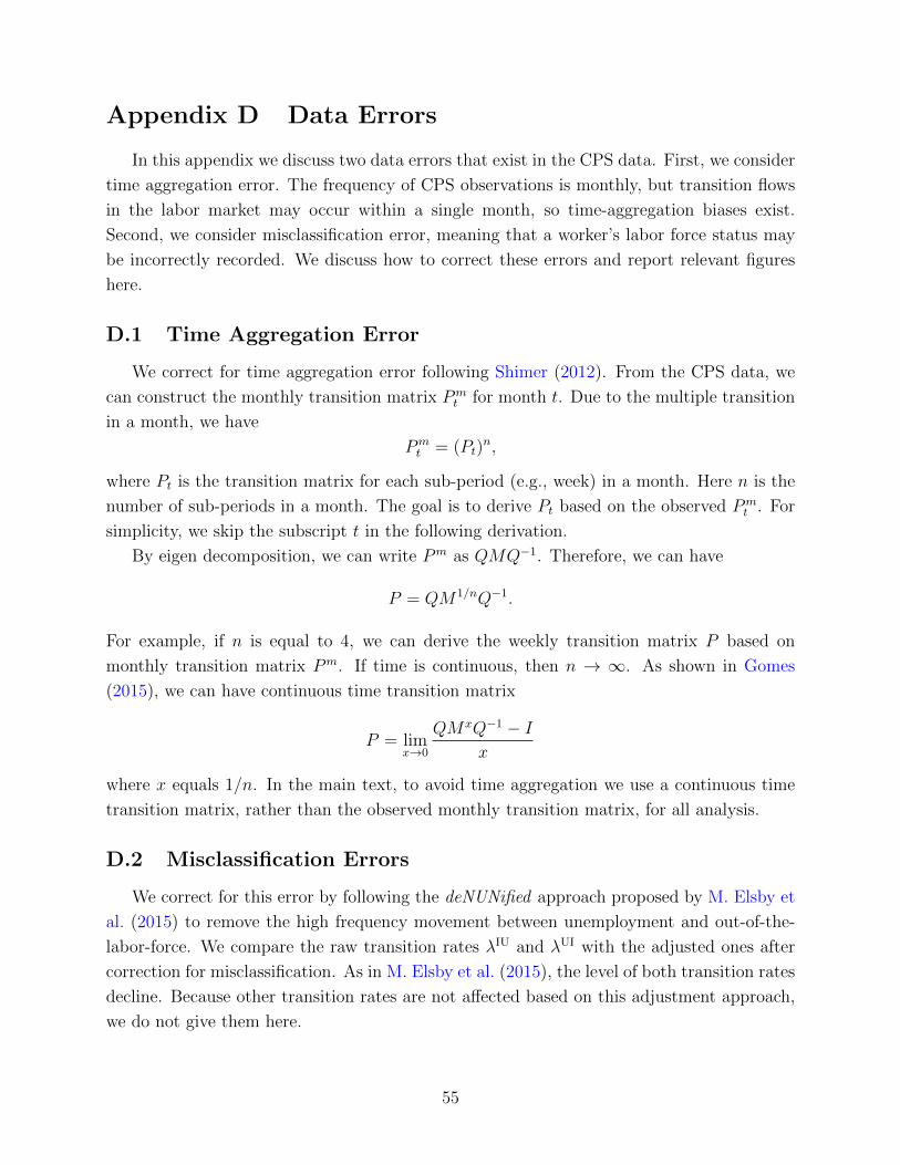
Appendix D Data Errors

In this appendix we discuss two data errors that exist in the CPS data. First, we consider

time aggregation error. The frequency of CPS observations is monthly, but transition flows

in the labor market may occur within a single month, so time-aggregation biases exist.

Second, we consider misclassification error, meaning that a worker’s labor force status may

be incorrectly recorded. We discuss how to correct these errors and report relevant figures

here.

D.1 Time Aggregation Error

We correct for time aggregation error following Shimer (2012). From the CPS data, we

can construct the monthly transition matrix Pmt for month t. Due to the multiple transition

in a month, we have

Pmt = (Pt)

n,

where Pt is the transition matrix for each sub-period (e.g., week) in a month. Here n is the

number of sub-periods in a month. The goal is to derive Pt based on the observed Pmt . For

simplicity, we skip the subscript t in the following derivation.

By eigen decomposition, we can write Pm as QMQ−1. Therefore, we can have

P = QM1/nQ−1.

For example, if n is equal to 4, we can derive the weekly transition matrix P based on

monthly transition matrix Pm. If time is continuous, then n → ∞. As shown in Gomes

(2015), we can have continuous time transition matrix

P = limx→0

QMxQ−1 − Ix

where x equals 1/n. In the main text, to avoid time aggregation we use a continuous time

transition matrix, rather than the observed monthly transition matrix, for all analysis.

D.2 Misclassification Errors

We correct for this error by following the deNUNified approach proposed by M. Elsby et

al. (2015) to remove the high frequency movement between unemployment and out-of-the-

labor-force. We compare the raw transition rates λIU and λUI with the adjusted ones after

correction for misclassification. As in M. Elsby et al. (2015), the level of both transition rates

decline. Because other transition rates are not affected based on this adjustment approach,

we do not give them here.

55

1978 1983 1988 1993 1998 2003 2008 2013 2018

0.20

0.25

0.30

0.35

0.40

0.45

0.50 AdjustedRaw

Non-White

1978 1983 1988 1993 1998 2003 2008 2013 2018

0.20

0.25

0.30

0.35

0.40

0.45

0.50AdjustedRaw

Young

1978 1983 1988 1993 1998 2003 2008 2013 2018

0.15

0.20

0.25

0.30

0.35

0.40

0.45 AdjustedRaw

No College Education

1978 1983 1988 1993 1998 2003 2008 2013 2018

0.20

0.25

0.30

0.35

0.40

0.45AdjustedRaw

Female

1978 1983 1988 1993 1998 2003 2008 2013 2018

0.15

0.20

0.25

0.30

0.35

0.40 AdjustedRaw

White

1978 1983 1988 1993 1998 2003 2008 2013 2018

0.15

0.20

0.25

0.30

0.35

AdjustedRaw

Experienced

1978 1983 1988 1993 1998 2003 2008 2013 2018

0.15

0.20

0.25

0.30

0.35 AdjustedRaw

Any College Education

1978 1983 1988 1993 1998 2003 2008 2013 2018

0.10

0.15

0.20

0.25

0.30

0.35 AdjustedRaw

Male

Figure D.1: λUI: Adjusted vs. Raw

Gray-shaded areas indicate NBER Recession periods. Data source: FRED & IPUMS-CPS.

56

1978 1983 1988 1993 1998 2003 2008 2013 20180.02

0.03

0.04

0.05

0.06

0.07

0.08

0.09 AdjustedRaw

Non-White

1978 1983 1988 1993 1998 2003 2008 2013 2018

0.04

0.06

0.08

0.10

0.12AdjustedRaw

Young

1978 1983 1988 1993 1998 2003 2008 2013 20180.015

0.020

0.025

0.030

0.035

0.040

0.045

AdjustedRaw

No College Education

1978 1983 1988 1993 1998 2003 2008 2013 2018

0.015

0.020

0.025

0.030

0.035

0.040

AdjustedRaw

Female

1978 1983 1988 1993 1998 2003 2008 2013 2018

0.015

0.020

0.025

0.030

0.035

0.040 AdjustedRaw

White

1978 1983 1988 1993 1998 2003 2008 2013 2018

0.010

0.015

0.020

0.025

0.030 AdjustedRaw

Experienced

1978 1983 1988 1993 1998 2003 2008 2013 2018

0.015

0.020

0.025

0.030

0.035

0.040

0.045

AdjustedRaw

Any College Education

1978 1983 1988 1993 1998 2003 2008 2013 2018

0.02

0.03

0.04

0.05

0.06

AdjustedRaw

Male

Figure D.2: λIU: Adjusted vs. Raw

Gray-shaded areas indicate NBER Recession periods. Data source: FRED & IPUMS-CPS.

57

Appendix E Deriving the Decomposition of the Un-

employment Rate

By the Taylor Theorem, we can rewrite the log difference in unemployment rate ut =

lnut− lnu∗t = lnu(Λt)−u(Λ∗t ) as a log-difference in transition rates λxt = lnλxt − lnλ∗xt , where

x ∈ X = {EU,EI,UE,UI, IE, IU}. To understand workers’ unemployment fluctuations,

lnut − ln ut, λ∗ijt will be the trend component in workers’ transition rate. When we discuss

a group of disadvantaged workers’ unemployment gap, lnugt − lnugt , we need to replace λ∗ijtwith the counterpart group of workers’ transition rate λg,ijt . The decomposition of the log

difference in unemployment rate, lnut − lnu∗t = lnu(Λt) − u(Λ∗t ), can be explicitly written

as

lnut − lnu∗t =∑x∈X

∂ lnu(Λt)

∂λxt

∣∣∣∣Λt=Λ∗

t

× λ∗xt · (lnλxt − lnλ∗xt ) + εt

= aUt (λ∗IEt + λ∗IUt )λ∗EUt · (lnλEU

t − lnλ∗EUt )

+ aUt λ∗IUt λ∗EI

t · (lnλEIt − lnλ∗EI

t )

+ aEt (λ∗IEt + λ∗IUt )λ∗UE · (lnλUEt − lnλ∗UE

t )

+ aEt λ∗IEt λ∗UI

t · (lnλUIt − lnλ∗UI

t )

+[aUt λ

∗EUt + aEt (λ∗UE

t + λ∗UIt )]λ∗IEt · (lnλIE

t − lnλ∗IEt )

+[aUt (λ∗EU

t + λ∗EIt ) + aEt λ

∗UEt

]λ∗IUt · (lnλIU

t − lnλ∗IUt ) + εt

=FEUt + FEI

t + FUEt + FUI

t + F IEt + F IU

t + εt,

(17)

where the coefficient aUt is equal to (1− u∗t )/U∗t and aE is equal to −u∗t/U∗t . Moreover,

U∗ = λ∗EUλ∗IU + λ∗IEλ∗EU + λ∗EIλ∗IU represents the total inflows to unemployment given

transition rates vector Λ∗t . Equation (17) gives the total log difference in unemployment,

lnut − lnu∗t , as consisting of six factors (F ) that depend on the log difference in transition

rate lnλt − lnλ∗xt . For example, FUE accounts for the part of lnut − lnu∗t that is driven

by the job-finding rate (i.e., lnλUEt − lnλ∗UE

t ). During recessions, FUEt will increase because

of the decline in job-finding rate, lnλUEt − ln λUE

t , and the negative component aEt . In the

calculations of unemployment gaps, FUEt would be positive because of the lower job-finding

rate of disadvantaged workers and aEt < 0. The error term εt accounts for the residual

between lnut − lnu∗t and the sum of these six factors.

E.1 Different Transition Events

In a given month, an unemployed worker may directly become employed (U→ E) or may

give up on job searching, then participate in the labor force again and find a job (U→ I→ E).

Similarly, an employed worker may become unemployed but continue to job search (E→ U)

58

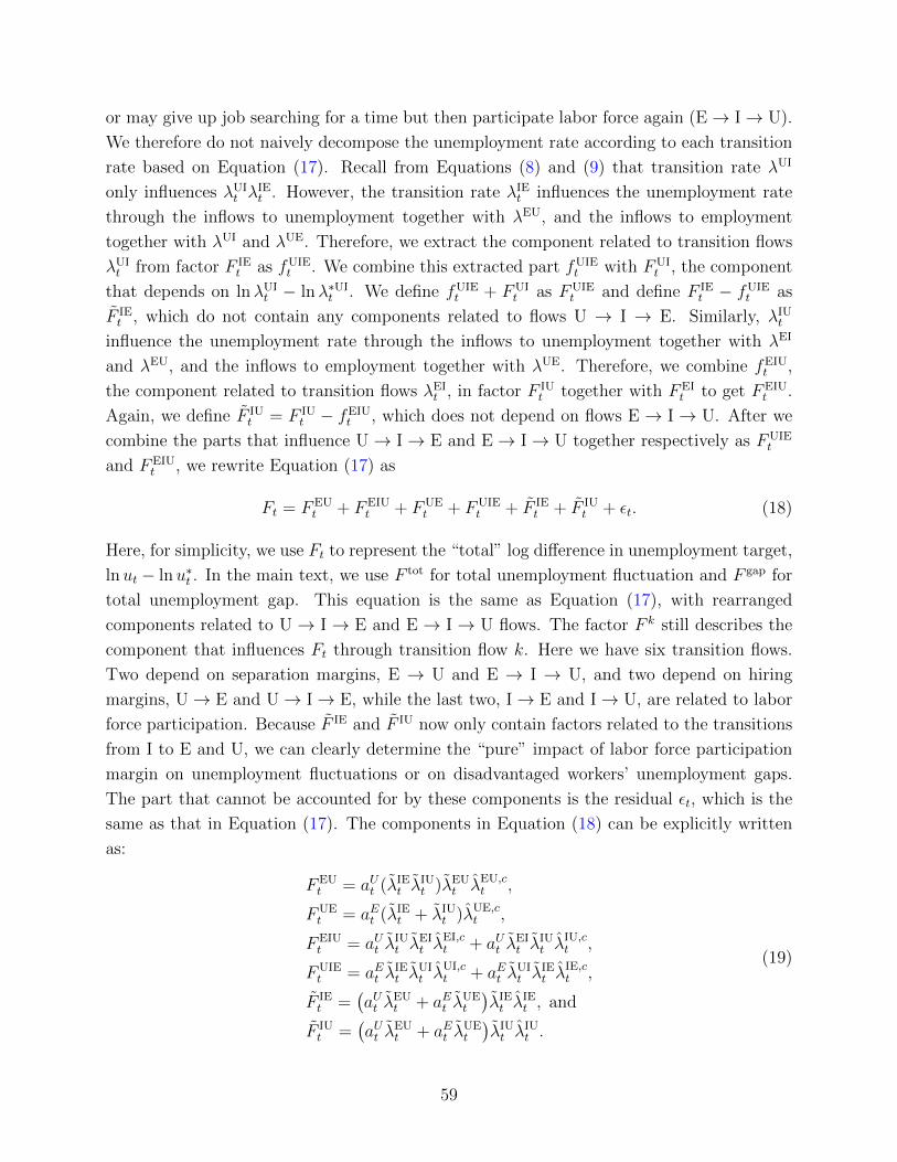
or may give up job searching for a time but then participate labor force again (E→ I→ U).

We therefore do not naively decompose the unemployment rate according to each transition

rate based on Equation (17). Recall from Equations (8) and (9) that transition rate λUI

only influences λUIt λ

IEt . However, the transition rate λIE

t influences the unemployment rate

through the inflows to unemployment together with λEU, and the inflows to employment

together with λUI and λUE. Therefore, we extract the component related to transition flows

λUIt from factor F IE

t as fUIEt . We combine this extracted part fUIE

t with FUIt , the component

that depends on lnλUIt − lnλ∗UI

t . We define fUIEt + FUI

t as FUIEt and define F IE

t − fUIEt as

F IEt , which do not contain any components related to flows U → I → E. Similarly, λIU

t

influence the unemployment rate through the inflows to unemployment together with λEI

and λEU, and the inflows to employment together with λUE. Therefore, we combine fEIUt ,

the component related to transition flows λEIt , in factor F IU

t together with FEIt to get FEIU

t .

Again, we define F IUt = F IU

t − fEIUt , which does not depend on flows E → I→ U. After we

combine the parts that influence U→ I→ E and E→ I→ U together respectively as FUIEt

and FEIUt , we rewrite Equation (17) as

Ft = FEUt + FEIU

t + FUEt + FUIE

t + F IEt + F IU

t + εt. (18)

Here, for simplicity, we use Ft to represent the “total” log difference in unemployment target,

lnut − lnu∗t . In the main text, we use F tot for total unemployment fluctuation and F gap for

total unemployment gap. This equation is the same as Equation (17), with rearranged

components related to U → I → E and E → I → U flows. The factor F k still describes the

component that influences Ft through transition flow k. Here we have six transition flows.

Two depend on separation margins, E → U and E → I → U, and two depend on hiring

margins, U→ E and U→ I→ E, while the last two, I→ E and I→ U, are related to labor

force participation. Because F IE and F IU now only contain factors related to the transitions

from I to E and U, we can clearly determine the “pure” impact of labor force participation

margin on unemployment fluctuations or on disadvantaged workers’ unemployment gaps.

The part that cannot be accounted for by these components is the residual εt, which is the

same as that in Equation (17). The components in Equation (18) can be explicitly written

as:

FEUt = aUt (λIE

t λIUt )λEU

t λEU,ct ,

FUEt = aEt (λIE

t + λIUt )λUE,c

t ,

FEIUt = aUt λ

IUt λ

EIt λ

EI,ct + aUt λ

EIt λ

IUt λ

IU,ct ,

FUIEt = aEt λ

IEt λ

UIt λ

UI,ct + aEt λ

UIt λ

IEt λ

IE,ct ,

F IEt =

(aUt λ

EUt + aEt λ

UEt

)λIEt λ

IEt , and

F IUt =

(aUt λ

EUt + aEt λ

UEt

)λIUt λ

IUt .

(19)

59

Table E.1: β Coefficient: Unemployment Fluctuations, Overall

Non-White Young No College All

E → U 0.167 0.158 0.213 0.206(0.014) (0.013) (0.012) (0.010)

E → I → U 0.058 0.022 0.056 0.079(0.014) (0.013) (0.010) (0.009)

U → E 0.490 0.570 0.503 0.512(0.013) (0.014) (0.012) (0.010)

U → I → E 0.289 0.242 0.232 0.204(0.012) (0.010) (0.009) (0.007)

I → E 0.005 0.021 0.008 0.008(0.000) (0.001) (0.001) (0.001)

I → U -0.003 -0.006 -0.004 -0.006(0.000) (0.001) (0.000) (0.000)

ε -0.006 -0.006 -0.007 -0.005(0.001) (0.001) (0.001) (0.001)

White Experienced With College All

E → U 0.218 0.246 0.216 0.206(0.011) (0.012) (0.012) (0.010)

E → I → U 0.085 0.097 0.110 0.079(0.009) (0.009) (0.010) (0.009)

U → E 0.522 0.464 0.523 0.512(0.011) (0.010) (0.013) (0.010)

U → I → E 0.177 0.197 0.155 0.204(0.007) (0.008) (0.008) (0.007)

I → E 0.008 0.004 0.007 0.008(0.001) (0.000) (0.001) (0.001)

I → U -0.006 -0.003 -0.007 -0.006(0.000) (0.000) (0.001) (0.000)

ε -0.005 -0.005 -0.004 -0.005(0.001) (0.001) (0.001) (0.001)

95% Confidence interval in brackets.

We give results (β and γ) based on the decomposition approach of Equation (18) as we did

in Tables 4 and 5.

Table E.1 gives estimated β based on Equation (18) for unemployment fluctuations. In

Table E.1, we also report standard errors so that importance of a specific transition rate

can be compared with other transition rates. The estimated β of the different worker types

share common features. First, the contribution of hiring margins to workers’ unemploy-

ment fluctuations (FUE + FUIE or FUE only) is significantly larger than that of separations

(FEU + FEIU or FEU only). Second, the role of direct inflows from U to E (FUE) is more

important than that of indirect inflows from U to I to E (FUIE). The same is true of the two

separation margins components FEU and FEIU. Third, direct inflows from I to E or from

I to U play trivial roles in unemployment fluctuations. Therefore, in the comparison with

separation or hiring margins, the pure impact of labor force participation (directly from I

60

Table E.2: Compositions of UnemploymentGap, Overall

Non-White Young No College

E → U 0.35 0.776 0.616(0.005) (0.008) (0.004)

E → I → U 0.433 1.237 0.196(0.006) (0.013) (0.004)

U → E 0.436 -0.188 0.116(0.006) (0.007) (0.006)

U → I → E -0.142 -0.746 0.064(0.005) (0.013) (0.003)

I → E -0.009 -0.048 0.035(0.001) (0.003) (0.001)

I → U -0.021 -0.029 0.001(0.001) (0.002) (0.000)

ε -0.048 -0.002 -0.027(0.002) (0.001) (0.001)

95% Confidence interval in brackets.

to U or E) in explaining unemployment fluctuations is very minor. Our analysis shows that

out-of-the-labor-force I is just a transient status when workers move between employment

and unemployment in a given month. Our results about I actually complement the findings

in M. Elsby et al. (2015) which emphasize the role of transition between I and U in unem-

ployment rate fluctuations. We show that IU or UI transition flows are important only when

I is a transient status between E and U.

Table E.2 shows the estimated fractions of the factors which depend on specific flows in

the total unemployment gap and the corresponding confidence interval. We can see that, for

all disadvantaged workers, the main factor in the unemployment gap is FEU. In particular,

the component FUE only accounts for 10 percent of the total unemployment gap for workers

with no college education, and its contribution is less than zero for young workers. This

finding for young workers is not surprising. It is consistent with the estimated parameter

in Table 2, which shows that young workers have higher job-finding rates compared with

experienced workers. However, for non-white workers 40 percent of the total unemployment

gap can be attributed to the contribution of FUE. Particularly, non-white workers’ ratio of

FUE to the total unemployment gap is significantly higher than that of FEU in total. We

also see that the impacts of FEIU and FUIE on the unemployment gap are different. For non-

white and young workers the unemployment gap is mainly caused by FEIU, a component

that belongs to the separation margin. However, FUIE, a component in the hiring margin,

does not contribute to the unemployment gap for all disadvantaged workers. As with the

estimated results from Table E.1, the pure labor force participation components F IE and F IU

do not account for any fraction of the unemployment gap. Transition flows related to not-in-

61

the-labor-force I are important only when I is a transient status for workers transiting from

E to U. Overall, hiring margins contribute to the unemployment gap for non-white workers,

while separation margins are the most crucial factors in explaining the unemployment gap

for all disadvantaged workers.

62

Appendix F Alternative Trend Measure

In this section we give estimation results based on the sample average as the trend

component, rather than the HP-filter trend. Based on Table F.1, the main results hold:

workers’ unemployment fluctuations can mainly be attributed to hiring margin rather than

separation margin. In addition, even though we use the sample average as the trend, the

small magnitude of βε shows again the accuracy of our decomposition approach.

Given the sample average as the trend, we show the separation margin for non-white

workers may contribute to their unemployment changes during normal times. When we use

the HP-filter trend in the main text, we find that the contribution of the separation margin

to unemployment fluctuations for non-white and young workers declines. Therefore, the

contribution of the separation margin to non-white workers’ unemployment fluctuations is

not significantly larger than that of other workers.

Moreover, based on the HP-filter trend, the contribution of the hiring margin to young

workers’ unemployment fluctuations is significantly larger than that for experienced workers.

Because using the HP-filter trend will increase the contribution of the hiring margin, based on

mean as the trend component, we have a lower bound for the contribution of the hiring margin

to non-white and young workers’ unemployment fluctuations. Fujita and Ramey (2009)

also addressed that the contribution of the hiring (separation) margin to unemployment

fluctuations is higher (lower) when we use the HP-filter trend. Our conclusion that hiring

influences disadvantaged workers’ unemployment fluctuations does not change even when we

use the HP-filter trend.

63

Table F.1: β Coefficient: Sample Average

Non-White Young No College All

λEU 0.31 0.209 0.207 0.245(0.014) (0.016) (0.012) (0.013)

λEI -0.004 -0.016 -0.029 -0.004(0.006) (0.009) (0.006) (0.006)

λUE 0.339 0.499 0.52 0.473(0.015) (0.02) (0.014) (0.016)

λUI 0.105 0.124 0.133 0.13(0.006) (0.007) (0.007) (0.005)

λIE 0.105 0.109 0.096 0.064(0.006) (0.009) (0.005) (0.004)

λIU 0.151 0.082 0.083 0.097(0.009) (0.012) (0.006) (0.006)

ε -0.006 -0.007 -0.01 -0.005(0.002) (0.002) (0.001) (0.001)

White Experienced With College All

λEU 0.248 0.246 0.2 0.245(0.014) (0.011) (0.012) (0.013)

λEI 0.003 -0.004 0.015 -0.004(0.006) (0.005) (0.006) (0.006)

λUE 0.49 0.475 0.562 0.473(0.016) (0.012) (0.015) (0.016)

λUI 0.12 0.138 0.089 0.13(0.005) (0.005) (0.006) (0.005)

λIE 0.05 0.052 0.059 0.064(0.004) (0.004) (0.007) (0.004)

λIU 0.094 0.099 0.087 0.097(0.005) (0.006) (0.008) (0.006)

ε -0.006 -0.006 -0.011 -0.005(0.001) (0.001) (0.001) (0.001)

Standard error in parentheses.

64

Appendix G β for Unemployment Gap

In the main text we use Equation (16) to derive the ratio of each factor to total unem-

ployment gap, so that we can determine the contribution of each factor to the unemployment

gap. The β coefficients in Equation (14) only reveal the importance of these factors to the

variation of unemployment gap, rather than the level of the gap. Therefore, we do not use

the β coefficient for analysis of the unemployment gap in the main text. This appendix gives

results for the β coefficients when we apply Equation (14) to the unemployment gap.

As we can see in Table G.1, variation in the unemployment gap is still mainly caused

by fluctuations in the separation factors FEU and FEIU for non-white and young workers.

For workers with no college education, 60 percent of the unemployment gap variation is ac-

counted for by the hiring margin, which only contributes around 20 percent to unemployment

gap. Table G.2 shows the β coefficients for the different recession periods. As in Table G.1,

variation in the unemployment gap is determined by the separation margin. Particularly,

the importance of the hiring margin for workers with no college education declines dur-

ing recessions (especially the Great Recession). Therefore, hiring margin only explains the

fluctuations in normal times for workers with no college education, rather than in recessions.

Although Figure 8 shows that the hiring margin contributes trivially to the unemployment

gap, the β coefficients for the hiring margin factors are even positive for young workers.

Moreover, the β coefficient for hiring margin is much larger than that for the separation

margin for those with no college education. Because β is the contribution of the fluctuations

of a factor to the variation, rather than the level, of the unemployment gap, β coefficients

are inconsistent with the features in Figure 8. For this reason we do not use β in the main

text for the unemployment gap.

65

Table G.1: β Coefficient: Unemployment Gap,Overall

Non-White Young No College

λEU 0.402 0.421 0.375[0.368, 0.436] [0.377, 0.465] [0.339, 0.411]

λEI 0.002 0.095 0.016[-0.017, 0.021] [0.069, 0.12] [-0.006, 0.038]

λUE 0.400 0.187 0.424[0.359, 0.441] [0.142, 0.232] [0.376, 0.471]

λUI 0.014 0.12 0.086[-0.003, 0.032] [0.098, 0.142] [0.066, 0.106]

λIE 0.100 -0.075 0.111[0.08, 0.119] [-0.107, -0.042] [0.088, 0.133]

λIU 0.156 0.27 0.023[0.134, 0.178] [0.234, 0.305] [-0.007, 0.054]

ε -0.074 -0.018 -0.035[-0.086, -0.062] [-0.029, -0.007] [-0.043, -0.028]

95% Confidence interval in brackets.

66

Table G.2: β Coefficient: Unemployment Gap, Recessions

Non-White 1980s 1990s 2000s Great Recession

λEU 0.365 0.292 0.512 0.199[0.178, 0.551] [0.168, 0.416] [0.273, 0.75] [0.039, 0.36]

λEI 0.165 0.065 0.009 0.099[0.078, 0.252] [-0.001, 0.13] [-0.117, 0.134] [0.012, 0.186]

λUE 0.374 0.466 0.346 0.3[0.207, 0.541] [0.258, 0.674] [0.107, 0.585] [0.142, 0.458]

λUI 0.094 0.106 0.121 0.13[0.041, 0.147] [0.044, 0.168] [0.012, 0.229] [0.028, 0.232]

λIE 0.051 0.026 0.089 0.079[-0.065, 0.167] [-0.055, 0.107] [-0.029, 0.207] [-0.008, 0.167]

λIU -0.024 0.097 0.008 0.134[-0.057, 0.104] [0.008, 0.185] [-0.161, 0.177] [0.027, 0.242]

ε -0.073 -0.051 -0.084 0.058[-0.127, -0.019] [-0.106, 0.004] [-0.148, -0.019] [-0.007, 0.124]

Young 1980s 1990s 2000s Great Recession

λEU 0.287 0.265 0.319 0.418[0.154, 0.42] [0.124, 0.406] [0.142, 0.497] [0.289, 0.548]

λEI 0.158 0.13 0.113 0.165[0.086, 0.23] [0.053, 0.207] [0.042, 0.184] [0.095, 0.236]

λUE 0.353 0.195 0.244 0.073[0.178, 0.528] [0.016, 0.374] [0.063, 0.425] [-0.079, 0.225]

λUI 0.066 0.162 0.142 0.141[0.014, 0.117] [0.067, 0.257] [0.048, 0.237] [0.079, 0.203]

λIE -0.139 0.024 -0.093 -0.138[-0.263, -0.015] [-0.115, 0.163] [-0.202, 0.016] [-0.215, -0.061]

λIU 0.301 0.195 0.279 0.327[0.158, 0.445] [0.04, 0.351] [0.152, 0.406] [0.234, 0.42]

ε -0.026 0.029 -0.004 0.013[-0.059, 0.007] [-0.017, 0.075] [-0.058, 0.051] [-0.029, 0.055]

No College 1980s 1990s 2000s Great Recession

λEU 0.412 0.37 0.245 0.496[0.295, 0.529] [0.252, 0.489] [0.108, 0.382] [0.327, 0.664]

λEI 0.053 0.094 0.043 0.138[-0.017, 0.124] [0.026, 0.162] [-0.022, 0.109] [0.059, 0.217]

λUE 0.399 0.41 0.474 0.217[0.232, 0.565] [0.215, 0.605] [0.287, 0.661] [0.028, 0.406]

λUI 0.004 0.07 0.174 0.047[-0.055, 0.063] [0.008, 0.132] [0.112, 0.237] [-0.036, 0.13]

λIE 0.135 0.034 0.026 0.098[0.075, 0.195] [-0.046, 0.114] [-0.028, 0.079] [0.003, 0.193]

λIU 0.036 0.049 0.053 0.027[-0.047, 0.119] [-0.064, 0.162] [-0.039, 0.145] [-0.098, 0.151]

ε -0.040 -0.028 -0.015 -0.022[-0.066, -0.013] [-0.055, -0.001] [-0.045, 0.015] [-0.051, 0.007]

95% Confidence interval in brackets.

67

Appendix H Definition of Young Workers

In the main text we define potential experience as age minus schooling years, defining

young workers as those with less than ten years of potential experience. However, given the

variation in years of schooling, the oldest of these “young” workers is 38. 20% of these young

workers are under 20, 60% are under 25, and more than 90% are under 30. In this appendix

we use age rather than potential experience. First, we use 18 years-old as the cut-off point,

defining workers who are 18 or younger as the young workers. We then use 20 as the cut-off

point to see if there is any difference.

Figure H.1 compares the unemployment rates of workers 18 (or 20) and younger with

older workers. We see there is still an unemployment gap, with workers 18 (or 20) and

younger showing a higher unemployment rate than older workers. Moreover, the dashed and

dotted lines show that the approximated unemployment rate based on Equation (10) still

tracks the observed unemployment rate well. Therefore, the unemployment gap is robust to

using age rather than potential experience to define young workers.

Figure H.2 compares the transition rates for young workers according to our definition

with the counterpart experienced workers. Figures H.3 and H.4 compare the transition rates

for workers aged 18 (and 20) and younger with the counterpart older workers. We find that

no matter whether using potential experience or age to define young workers, the dynamics

and the features of the transition rates do not change. For example, the entry rates to

unemployment (from the employment or the out-of-the-labor-force) are higher for younger

workers than for the counterpart older workers. Moreover, the level of job-finding rates

for younger workers are similar to those of older workers and decrease significantly during

recessions. Therefore, we confirm that transition rates have similar features whether using

potential experience or age to define young workers.

Because the unemployment rates and transition flows have the same features and dynam-

ics when using age to define young workers, the source of the fluctuations and unemployment

gap should also be similar to our analysis in the main text. Table H.1 gives results for workers

18 (or 20) and younger. For the source of fluctuations, we find that the decline in job-finding

rates still explain around 50% of the fluctuations in the unemployment rates. This is consis-

tent with the findings for young workers in the main text. In addition, for the unemployment

gap between younger workers and older workers we find that entry rates to unemployment

(i.e., λEU and λIU) and transition rates from employment to out-of-the-labor-force are the

main sources of the unemployment gap. Particularly, the separation rate λEU accounts for

most of the unemployment gap. These features are similar to those found in the main text,

with the only difference being that the contribution to the unemployment gap of λIU declines

and the contribution of λIE increases.

So, whether we use years of potential experience or solely age to define young work-

68

ers, we reach similar conclusions about the sources of unemployment fluctuations and the

unemployment gap.

1977 1982 1987 1992 1997 2002 2007 2012 2017

0.05

0.10

0.15

0.20

0.25

0.30

Younger than 19

Older than 19

Unemployment Rate: 18 Years as Cut-Off

1977 1982 1987 1992 1997 2002 2007 2012 2017

0.05

0.10

0.15

0.20

0.25

Younger than 21

Older than 21

Unemployment Rate: 20 Years as Cut-Off

Figure H.1: Unemployment Rate: Young Workers

Solid lines represent the observed unemployment rate while dashed and dotted lines are the approximated

unemployment rate based on Equation (10), i.e., Shimer’s approach.

1978 1983 1988 1993 1998 2003 2008 2013 20180.010

0.015

0.020

0.025

0.030

0.035

0.040λEU: YoungλEU: Experienced

λEU

1978 1983 1988 1993 1998 2003 2008 2013 20180.020

0.025

0.030

0.035

0.040

0.045

0.050

0.055

λEI: YoungλEI: Experienced

λEI

1978 1983 1988 1993 1998 2003 2008 2013 2018

0.20

0.25

0.30

0.35

0.40

0.45

0.50

0.55 λUE: YoungλUE: Experienced

λUE

1978 1983 1988 1993 1998 2003 2008 2013 2018

0.15

0.20

0.25

0.30

0.35

0.40λUI: YoungλUI: Experienced

λUI

1978 1983 1988 1993 1998 2003 2008 2013 2018

0.04

0.06

0.08

0.10

0.12

0.14λ IE: Youngλ IE: Experienced

λIE

1978 1983 1988 1993 1998 2003 2008 2013 2018

0.02

0.04

0.06

0.08

λ IU: Youngλ IU: Experienced

λIU

Figure H.2: Transition Rates: Young Workers

Black solid lines are the observed transition rates for young workers while green-dashed lines are those for

experienced workers.

69

1977 1982 1987 1992 1997 2002 2007 2012 20170.01

0.02

0.03

0.04

0.05

0.06

0.07

0.08

0.09 Younger than 19: λEUOlder than 19: λEU

λEU

1977 1982 1987 1992 1997 2002 2007 2012 2017

0.05

0.10

0.15

0.20

Younger than 19: λEIOlder than 19: λEI

λEI

1977 1982 1987 1992 1997 2002 2007 2012 2017

0.2

0.3

0.4

0.5

0.6

0.7

0.8 Younger than 19: λUEOlder than 19: λUE

λUE

1977 1982 1987 1992 1997 2002 2007 2012 20170.1

0.2

0.3

0.4

0.5

0.6Younger than 19: λUIOlder than 19: λUI

λUI

1977 1982 1987 1992 1997 2002 2007 2012 20170.025

0.050

0.075

0.100

0.125

0.150

0.175

0.200 Younger than 19: λ IEOlder than 19: λ IE

λIE

1977 1982 1987 1992 1997 2002 2007 2012 2017

0.02

0.04

0.06

0.08

0.10Younger than 19: λ IUOlder than 19: λ IU

λIU

Figure H.3: Transition Rates: Workers 18 and Younger

Black solid lines are the observed transition rates for workers age 18 or younger while green-dashed lines

those for older workers.

70

1977 1982 1987 1992 1997 2002 2007 2012 20170.01

0.02

0.03

0.04

0.05

0.06

0.07

0.08 Younger than 21: λEUOlder than 21: λEU

λEU

1977 1982 1987 1992 1997 2002 2007 2012 2017

0.02

0.04

0.06

0.08

0.10

0.12

0.14

0.16Younger than 21: λEIOlder than 21: λEI

λEI

1977 1982 1987 1992 1997 2002 2007 2012 2017

0.2

0.3

0.4

0.5

0.6

0.7

0.8Younger than 21: λUEOlder than 21: λUE

λUE

1977 1982 1987 1992 1997 2002 2007 2012 20170.1

0.2

0.3

0.4

0.5

0.6Younger than 21: λUIOlder than 21: λUI

λUI

1977 1982 1987 1992 1997 2002 2007 2012 20170.025

0.050

0.075

0.100

0.125

0.150

0.175

0.200 Younger than 21: λ IEOlder than 21: λ IE

λIE

1977 1982 1987 1992 1997 2002 2007 2012 2017

0.02

0.04

0.06

0.08

0.10Younger than 21: λ IUOlder than 21: λ IU

λIU

Figure H.4: Transition Rates: Workers 20 and Younger

Black solid lines are the observed transition rates for workers age 20 or younger while green-dashed lines are

those for older workers.

71

Table H.1: The β Coefficients and r Ratio

Fluctuation: β Coefficient 18 and Younger 20 and Younger

λEU 0.115 0.140(0.017) (0.014)

λEI 0.013 -0.020(0.014) (0.010)

λUE 0.501 0.533(0.021) (0.017)

λUI 0.049 0.072(0.013) (0.011)

λIE 0.271 0.213(0.012) (0.010)

λIU 0.062 0.074(0.018) (0.014)

ε -0.012 -0.012(0.003) (0.003)

Gap: r Ratio 18 and Younger 20 and Younger

λEU 0.615 0.690(0.006) (0.005)

λEI 0.489 0.453(0.004) (0.003)

λUE -0.058 -0.093(0.005) (0.004)

λUI -0.169 -0.153(0.003) (0.003)

λIE -0.182 -0.248(0.004) (0.003)

λIU 0.283 0.350(0.004) (0.003)

ε 0.022 0.001(0.003) (0.002)

Standard errors in parentheses.

72

Appendix I Heterogeneity within Demographic Groups

This appendix provides more detail on sources of heterogeneity within our six demo-

graphic groups. Disadvantaged workers may differ from their counterpart groups across a

wide variety of dimensions such as geography, occupation, and other demographic charac-

teristics. We investigate whether these other dimensions can explain the group differences

found in the main results.

We begin by investigating demographic variation. Table I.1 shows the percentages of

non-white workers, those with no college, female, and young workers in each demographic

subgroup. For example, among non-white workers 55 percent have no college experience.

The last column in Table I.1 gives the percentages of non-white, without college, female,

and young workers in the total sample. According to Table I.1, the percentages of workers

with these demographic characteristics are similar across the eight worker groups. Thus, it

is not the case that other sources of demographic heterogeneity are driving the differences

we observe between groups in the main results.

Next we turn to geography and occupations. If disadvantaged workers are clustered

in locations with worse labor markets or are more likely to be employed in jobs that are

more volatile, these characteristics could lead to worse labor market outcomes. To formally

investigate the role these characteristics play, we use an analysis similar to Albanesi and

Sahin (2018), who analyze how composition has affected female and male unemployment

rates. In particular, we construct counterfactual transition rates and unemployment rates,

using the counterpart groups’ distribution across a characteristic to construct a re-weighted

flow or unemployment rate. This tells us how much of the difference in the flow is due

to differences in transition rates within groups versus differences in composition between

groups.

First, we compute the group share in each cell (e.g., occupation or state), which we then

use to weight the labor market flows and the unemployment rate within the cell. Specifically,

we calculate

λxt =∑i∈I

witλxit, (20)

where x ∈ {EU,EI,UE,UI, IE, IU}, i represents the characteristics (occupation, location,

etc) and t represents the period. For example, i may represent different occupations. Here,

wit means the percentage of workers with characteristic i and λit means the transition flows

for workers with characteristic i. Similarly, the formula for weighted unemployment rate is

ut =∑i∈I

wituit, (21)

where uit is the unemployment rate for workers with characteristic i.

Next, we construct the weights for each disadvantaged group’s counterpart group (wCit ),

73

which we then use to construct the counterfactual flow and unemployment rates. We then

compute the following measure:

errx =

∑Tt=0(ln λx,Ct − ln λxt )

2

T× 100

erru =

∑Tt=0(ln ux,Ct − ln uxt )

2

T× 100

(22)

which are the logarithm root mean square errors (RMSE) between the counterfactual tran-

sition flows ln λx,Ct and unemployment rates ln ux,Ct compared with those observed (ln λxt and

ln uxt ). We use the logarithms of these variables to avoid the issue that transition flow rates

and unemployment rates differ in magnitudes. For example, λEU is only one-quarter of λUE,

so if we did not use the logarithm of λEU and merely compute the RMSE, the value would

be small and could not accurately measure the difference between the observed and counter-

factual λEU. Because all variables are now in logarithm, errx and erru represent the relative

changes between the observed flow rates (or unemployment rates) and counterfactual ones.

I.1 Analysis

In addition to the four characteristics (non-white, young, female, and no college educa-

tion), we also consider the decomposition by age, occupation and location in the analysis.

For the decomposition by age, we follow Albanesi and Sahin (2018) and use three groups:

below 24, 24 to 55, and greater than 55. Table I.2 shows the relative differences (in percent-

ages) for transition flows and unemployment comparing the observed and counterfactual.

Recall the counterfactual transition flow and unemployment rates are constructed by re-

placing the compositions with their counterpart advantaged workers. Table I.2 shows that

when non-white workers have the same compositions as white workers, transition rates and

unemployment rates are similar to those originally observed. Therefore, the impact of being

non-white on the transition and unemployment rates is quite significant.

Table I.2 shows that the relative differences are large for λIU considering compositions and

λUE considering occupation compositions. Figure I.1 shows these two series and compares

the original and the counterfactual. Based on Figure I.1, we find they are close to each other.

In the following discussion, we therefore use 1.5%, which is the relative difference for λIU

considering age composition as the criterion to determine the significance of the effect of the

decomposition.

Table I.3 gives the relative differences for workers with no college. Unlike for non-white

workers, decomposition by age and occupation significantly affects the transition flow rates

and unemployment rates for the workers with no college. Figure I.2 plots those flows or

unemployment rate with relative differences greater than 1.5%.

We find that when the workers with no college have the same age composition as workers

74

with any college, transition rates from employment to out-of-the-labor-force and from out-of-

the-labor-force into the labor force both declined. Despite the age decomposition affecting

transition rates, these difference did not cause significant changes in unemployment rates

(the relative difference is only 0.23%). In addition to age composition, Figure I.2 shows

that when the workers with no college have the same occupational composition as that of

workers with any college, exit rates from employment become lower while entry rates into

employment become higher. The influence of occupational decomposition on transition flows

also causes the unemployment rate for workers with no college to decline.

Table I.4 gives the relative differences for young workers. Decomposition by age and oc-

cupation significantly affect transition flow rates and unemployment rates for young workers.

It is not surprising that age composition causes difference in transition flow and unemploy-

ment rates as we define young workers by workers’ age and schooling. Therefore, this finding

confirms that our definition of young workers can reveal workers’ age. Figure I.3 plots the

flows or unemployment rate with a relative difference greater than 1.5% after we consider

the occupational composition.

When young workers have the same occupational composition as experienced workers,

the exit rate from employment increases while the entry rate into employment decreases.

Therefore, the occupational composition causes young workers’ unemployment to increase,

showing that young workers and experienced worker work in different occupations.

These results show that occupational segregation by education and age can explain part

of the differences in transition rates between groups. This could be due to searching in

different labor markets, or to differences in qualifications or search ability. However, for

non-white workers, differences in occupational segregation do not appear to affect transition

rates.

I.2 Controlling for Occupation & Geography

In the previous analysis we analyzed how occupation, location, and age decomposition

affected transition flows and unemployment rates for each group of disadvantaged workers.

As we showed show that occupational composition does affect transition flows and unem-

ployment rates, so one may wonder whether the features found in Table 2 still hold.

We therefore redo the regression, controlling for occupation together with location (by

state of residence). However we do not consider age decomposition as it can be captured by

the regression for young workers. The estimation equation is

ln yt =β0 + βd1d + βr lnut + βdr (lnut × 1d) +∑m

am1m

+ βocc1occ + βocc,d(1occ × 1d) + βs1State + βs,d(1State × 1d) + εt.

(23)

where 1d is an indicator for the disadvantaged demographic group, and 1m are month-by-year

75

fixed effects. Here, we add 1occ as the indicator for occupation and 1s as the indicator for

the workers’ state of residence. Again, we use yt to represent either the unemployment rates

or transition rates.

Table I.5 gives regression results after controlling for occupation. We find that the results

are mainly similar to those reported in Table 2 for minority workers. This shows that the

impact of race on transition flows and unemployment rates is quite universal and will not

change, even controlling for occupation or state. For workers with no college, after controlling

for occupation, the transition flows between unemployment and out-of-the-labor-force (λUI

and λIU) become more volatile than for counterpart workers with college experience. In

Table 2 these two transitions flows for workers with no college are higher than those for

workers with any college, but they become higher after we control for occupation. Because

education level limits the occupations in which workers can search for jobs, we believe this

can be attributed to the fact that workers with no college experience search and work in

different occupations than do workers with college degrees. Therefore, after we control for

occupation, the magnitude of the impact of attending college or not on λUI and λIU changes.

There do exist some differences for young workers. Except for the separation rate λEU,

the signs for the other transition rates are different from those in Table 2. For example,

in Table 2 young workers have a higher entry rate to employment (λUE and λIE), while in

Table I.6 young workers’ entry rate to employment is lower than that of experienced workers

after controlling for occupation. When we do not control for occupation, young workers

see higher employment entry rates. This difference indicated that the labor market young

workers search for jobs is segregated and different from those for experienced workers.

Additionally, after controlling for occupation, the entry rates to unemployment from out-

of-the-labor-force (λIU) and the employment entry rate (λEU + λEI) both become higher for

young workers. We believe this can be attributed to the labor markets for young workers’

search being different from those for experienced workers. However, we cannot conclude that

the impact of age and potential experience on transition flows changes after controlling for

occupation. As years of work experience can limit the occupations in which a worker can

search, occupational difference therefore matters here, and the different labor markets for

young workers’ search will depend on their years of experience.

Table I.6 gives the results after we control for both occupation and workers’ state of

residence. We find results similar to those in Table I.5. Therefore, location does not cause

significant differences in transition flows and unemployment rate.

76

1978 1983 1988 1993 1998 2003 2008 2013 2018

0.015

0.020

0.025

0.030

0.035

0.040

0.045

0.050

λIU: Age Composition

1978 1983 1988 1993 1998 2003 2008 2013 20180.12

0.14

0.16

0.18

0.20

0.22

0.24

0.26

0.28

λUE: Occupational Composition

Figure I.1: Transition Rates: Non-White Workers

Black solid lines are the original observed series while green-dashed lines are the counterfactual series given

the composition of counterpart advantaged workers.

77

1978 1983 1988 1993 1998 2003 2008 2013 2018

0.0225

0.0250

0.0275

0.0300

0.0325

0.0350

0.0375

λEI: Age Composition

1978 1983 1988 1993 1998 2003 2008 2013 20180.030

0.035

0.040

0.045

0.050

0.055

λIE: Age Composition

1978 1983 1988 1993 1998 2003 2008 2013 20180.0100

0.0125

0.0150

0.0175

0.0200

0.0225

0.0250

0.0275

λIU: Age Composition

1978 1983 1988 1993 1998 2003 2008 2013 20180.50

0.55

0.60

0.65

0.70

0.75

0.80

λEE: Occupational Composition

1978 1983 1988 1993 1998 2003 2008 2013 2018

0.010

0.015

0.020

0.025

0.030

0.035

0.040

λEU: Occupational Composition

1978 1983 1988 1993 1998 2003 2008 2013 2018

0.20

0.25

0.30

0.35

0.40

0.45

λEI: Occupational Composition

1978 1983 1988 1993 1998 2003 2008 2013 20180.02

0.03

0.04

0.05

0.06

0.07

0.08

0.09

λUE: Occupational Composition

1978 1983 1988 1993 1998 2003 2008 2013 2018

0.0015

0.0020

0.0025

0.0030

0.0035

0.0040

0.0045

λIE: Occupational Composition

1978 1983 1988 1993 1998 2003 2008 2013 2018

0.10

0.15

0.20

0.25

0.30

0.35

0.40

u: Occupational Composition

Figure I.2: Transition Rates: No College Degree

Black solid lines are the original observed series while green-dashed lines are the counterfactual series given

the composition of counterpart advantaged workers.

78

1978 1983 1988 1993 1998 2003 2008 2013 2018

0.55

0.60

0.65

0.70

0.75

λEE: Occupational Composition

1978 1983 1988 1993 1998 2003 2008 2013 2018

0.01

0.02

0.03

0.04

0.05

0.06

λEU: Occupational Composition

1978 1983 1988 1993 1998 2003 2008 2013 20180.20

0.25

0.30

0.35

0.40

0.45

λEI: Occupational Composition

1978 1983 1988 1993 1998 2003 2008 2013 20180.02

0.04

0.06

0.08

0.10

0.12

λUE: Occupational Composition

1978 1983 1988 1993 1998 2003 2008 2013 2018

0.005

0.010

0.015

0.020

0.025

λIE: Occupational Composition

1978 1983 1988 1993 1998 2003 2008 2013 2018

0.15

0.20

0.25

0.30

0.35

0.40

0.45

u: Occupational Composition

Figure I.3: Transition Rates: Young Workers

Black solid lines are the original observed series while green-dashed lines are the counterfactual series given

the composition of counterpart advantaged workers.

Table I.1: Compositions: Each Subgroup

White Non-White College Above College Below Experienced Young All

Non-White − − 16% 17% 16% 20% 17%College Below 53% 55% − − 54% 51% 53%Young 25% 31% 27% 25% − − 26%Female 52% 54% 51% 53% 53% 50% 52%

Percentages of non-white workers, those with no college, and young workers in each subgroup and intotal workers.

79

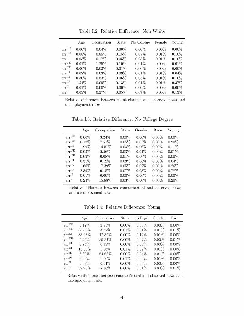
Table I.2: Relative Difference: Non-White

Age Occupation State No College Female Young

errEE 0.00% 0.04% 0.00% 0.00% 0.00% 0.00%errEU 0.08% 0.85% 0.15% 0.07% 0.01% 0.10%errEI 0.03% 0.17% 0.05% 0.03% 0.01% 0.10%errUE 0.01% 1.25% 0.10% 0.01% 0.00% 0.01%errUU 0.00% 0.02% 0.01% 0.00% 0.00% 0.00%errUI 0.02% 0.03% 0.09% 0.01% 0.01% 0.04%errIE 0.80% 0.83% 0.06% 0.03% 0.01% 0.10%errIU 1.54% 0.09% 0.13% 0.01% 0.01% 0.37%errII 0.01% 0.00% 0.00% 0.00% 0.00% 0.00%erru 0.09% 0.27% 0.05% 0.07% 0.00% 0.13%

Relative differences between counterfactual and observed flows andunemployment rates.

Table I.3: Relative Difference: No College Degree

Age Occupation State Gender Race Young

errEE 0.00% 3.24% 0.00% 0.00% 0.00% 0.00%errEU 0.12% 7.51% 0.05% 0.03% 0.00% 0.20%errEI 1.99% 14.57% 0.03% 0.06% 0.00% 0.11%errUE 0.03% 2.56% 0.03% 0.01% 0.00% 0.01%errUU 0.02% 0.08% 0.01% 0.00% 0.00% 0.00%errUI 0.31% 0.12% 0.03% 0.06% 0.00% 0.04%errIE 1.66% 17.39% 0.05% 0.02% 0.00% 0.26%errIU 2.39% 0.15% 0.07% 0.03% 0.00% 0.78%errII 0.01% 0.00% 0.00% 0.00% 0.00% 0.00%erru 0.23% 15.88% 0.03% 0.00% 0.00% 0.20%

Relative difference between counterfactual and observed flowsand unemployment rate.

Table I.4: Relative Difference: Young

Age Occupation State College Gender Race

errEE 0.17% 2.83% 0.00% 0.00% 0.00% 0.00%errEU 33.86% 3.77% 0.01% 0.31% 0.01% 0.01%errEI 83.23% 12.30% 0.00% 0.12% 0.01% 0.00%errUE 0.96% 39.32% 0.00% 0.02% 0.00% 0.01%errUU 0.84% 0.12% 0.00% 0.00% 0.00% 0.00%errUI 13.38% 1.26% 0.01% 0.02% 0.01% 0.00%errIE 3.33% 64.68% 0.00% 0.04% 0.01% 0.00%errIU 6.92% 1.00% 0.01% 0.02% 0.01% 0.00%errII 0.09% 0.01% 0.00% 0.00% 0.00% 0.00%erru 37.90% 8.30% 0.00% 0.31% 0.00% 0.01%

Relative difference between counterfactual and observed flows andunemployment rate.

80

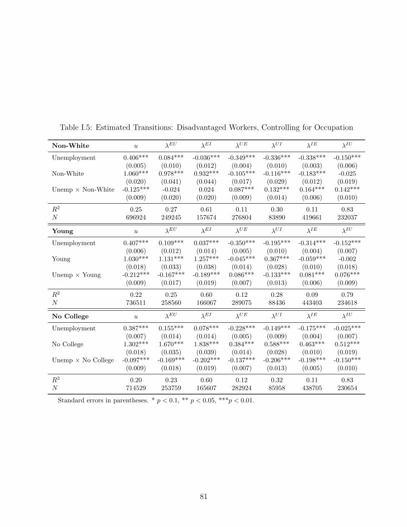
Table I.5: Estimated Transitions: Disadvantaged Workers, Controlling for Occupation

Non-White u λEU λEI λUE λUI λIE λIU

Unemployment 0.406*** 0.084*** -0.036*** -0.349*** -0.336*** -0.338*** -0.150***(0.005) (0.010) (0.012) (0.004) (0.010) (0.003) (0.006)

Non-White 1.060*** 0.978*** 0.932*** -0.105*** -0.116*** -0.183*** -0.025(0.020) (0.041) (0.044) (0.017) (0.029) (0.012) (0.019)

Unemp × Non-White -0.125*** -0.024 0.024 0.087*** 0.132*** 0.164*** 0.142***(0.009) (0.020) (0.020) (0.009) (0.014) (0.006) (0.010)

R2 0.25 0.27 0.61 0.11 0.30 0.11 0.83N 696924 249245 157674 276804 83890 419661 232037

Young u λEU λEI λUE λUI λIE λIU

Unemployment 0.407*** 0.109*** 0.037*** -0.350*** -0.195*** -0.314*** -0.152***(0.006) (0.012) (0.014) (0.005) (0.010) (0.004) (0.007)

Young 1.030*** 1.131*** 1.257*** -0.045*** 0.367*** -0.059*** -0.002(0.018) (0.033) (0.038) (0.014) (0.028) (0.010) (0.018)

Unemp × Young -0.212*** -0.167*** -0.189*** 0.086*** -0.133*** 0.081*** 0.076***(0.009) (0.017) (0.019) (0.007) (0.013) (0.006) (0.009)

R2 0.22 0.25 0.60 0.12 0.28 0.09 0.79N 736511 258560 166067 289075 88436 443403 234618

No College u λEU λEI λUE λUI λIE λIU

Unemployment 0.387*** 0.155*** 0.078*** -0.228*** -0.149*** -0.175*** -0.025***(0.007) (0.014) (0.014) (0.005) (0.009) (0.004) (0.007)

No College 1.302*** 1.670*** 1.838*** 0.384*** 0.588*** 0.463*** 0.512***(0.018) (0.035) (0.039) (0.014) (0.028) (0.010) (0.019)

Unemp × No College -0.097*** -0.169*** -0.202*** -0.137*** -0.206*** -0.198*** -0.150***(0.009) (0.018) (0.019) (0.007) (0.013) (0.005) (0.010)

R2 0.20 0.23 0.60 0.12 0.32 0.11 0.83N 714529 253759 165607 282924 85958 438705 230654

Standard errors in parentheses. * p < 0.1, ** p < 0.05, ***p < 0.01.

81

Table I.6: Estimated Transitions: Disadvantaged Workers, Controlling for Occupation andState

Non-White u λEU λEI λUE λUI λIE λIU

Unemployment 0.403*** 0.084*** -0.020* -0.348*** -0.330*** -0.333*** -0.154***(0.005) (0.009) (0.012) (0.004) (0.009) (0.003) (0.006)

Non-White 0.911*** 0.597*** 0.596*** -0.217*** -0.360*** -0.256*** -0.148***(0.024) (0.048) (0.051) (0.022) (0.036) (0.016) (0.025)

Unemp × Non-White -0.129*** 0.005 0.016 0.092*** 0.126*** 0.164*** 0.145***(0.009) (0.018) (0.019) (0.009) (0.013) (0.006) (0.010)

R2 0.31 0.36 0.66 0.17 0.37 0.14 0.84N 696924 249245 157674 276804 83890 419661 232037

Young u λEU λEI λUE λUI λIE λIU

Unemployment 0.404*** 0.111*** 0.040*** -0.348*** -0.189*** -0.310*** -0.156***(0.006) (0.011) (0.013) (0.005) (0.009) (0.004) (0.006)

Young 1.105*** 1.143*** 1.227*** -0.106*** 0.275*** -0.049*** -0.003(0.023) (0.043) (0.047) (0.019) (0.034) (0.015) (0.025)

Unemp × Young -0.211*** -0.160*** -0.175*** 0.086*** -0.136*** 0.082*** 0.076***(0.008) (0.015) (0.017) (0.007) (0.013) (0.005) (0.009)

R2 0.27 0.35 0.65 0.18 0.35 0.13 0.81N 736511 258560 166067 289075 88436 443403 234618

No College u λEU λEI λUE λUI λIE λIU

Unemployment 0.385*** 0.168*** 0.084*** -0.226*** -0.143*** -0.173*** -0.032***(0.007) (0.013) (0.014) (0.005) (0.008) (0.003) (0.007)

No College 1.166*** 1.511*** 1.744*** 0.319*** 0.628*** 0.435*** 0.380***(0.025) (0.047) (0.049) (0.019) (0.034) (0.014) (0.025)

Unemp × No College -0.097*** -0.180*** -0.194*** -0.138*** -0.207*** -0.196*** -0.144***(0.009) (0.017) (0.018) (0.007) (0.013) (0.005) (0.009)

R2 0.25 0.33 0.65 0.19 0.39 0.15 0.84N 714529 253759 165607 282924 85958 438705 230654

Standard errors in parentheses. * p < 0.1, ** p < 0.05, ***p < 0.01.

82

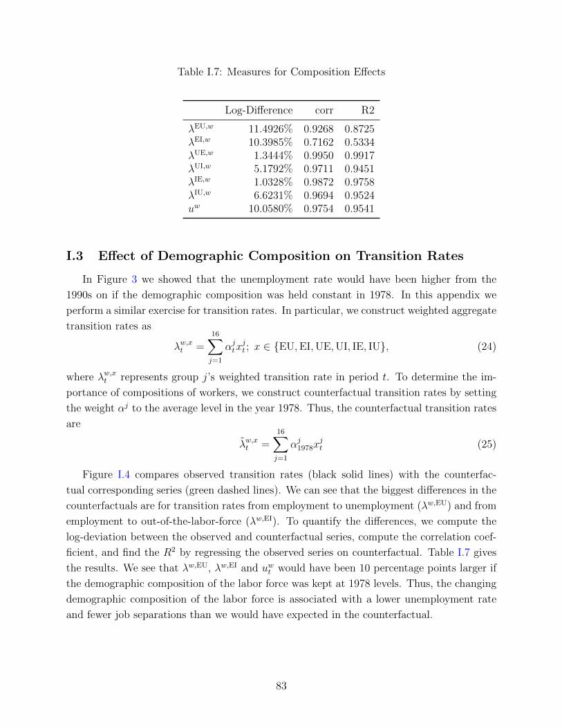
Table I.7: Measures for Composition Effects

Log-Difference corr R2

λEU,w 11.4926% 0.9268 0.8725λEI,w 10.3985% 0.7162 0.5334λUE,w 1.3444% 0.9950 0.9917λUI,w 5.1792% 0.9711 0.9451λIE,w 1.0328% 0.9872 0.9758λIU,w 6.6231% 0.9694 0.9524uw 10.0580% 0.9754 0.9541

I.3 Effect of Demographic Composition on Transition Rates

In Figure 3 we showed that the unemployment rate would have been higher from the

1990s on if the demographic composition was held constant in 1978. In this appendix we

perform a similar exercise for transition rates. In particular, we construct weighted aggregate

transition rates as

λw,xt =16∑j=1

αjtxjt ; x ∈ {EU,EI,UE,UI, IE, IU}, (24)

where λw,xt represents group j’s weighted transition rate in period t. To determine the im-

portance of compositions of workers, we construct counterfactual transition rates by setting

the weight αj to the average level in the year 1978. Thus, the counterfactual transition rates

are

λw,xt =16∑j=1

αj1978xjt (25)

Figure I.4 compares observed transition rates (black solid lines) with the counterfac-

tual corresponding series (green dashed lines). We can see that the biggest differences in the

counterfactuals are for transition rates from employment to unemployment (λw,EU) and from

employment to out-of-the-labor-force (λw,EI). To quantify the differences, we compute the

log-deviation between the observed and counterfactual series, compute the correlation coef-

ficient, and find the R2 by regressing the observed series on counterfactual. Table I.7 gives

the results. We see that λw,EU, λw,EI and uwt would have been 10 percentage points larger if

the demographic composition of the labor force was kept at 1978 levels. Thus, the changing

demographic composition of the labor force is associated with a lower unemployment rate

and fewer job separations than we would have expected in the counterfactual.

83

1980 1985 1990 1995 2000 2005 2010 2015 20200.012

0.014

0.016

0.018

0.020

0.022

0.024

0.026

0.028

λEU,w

1980 1985 1990 1995 2000 2005 2010 2015 2020

0.028

0.030

0.032

0.034

0.036

0.038

0.040

0.042

0.044

λEI,w

1980 1985 1990 1995 2000 2005 2010 2015 2020

0.20

0.25

0.30

0.35

0.40

0.45

0.50

0.55

λUE,w

1980 1985 1990 1995 2000 2005 2010 2015 2020

0.16

0.18

0.20

0.22

0.24

0.26

0.28

0.30

λUI,w

1980 1985 1990 1995 2000 2005 2010 2015 2020

0.020

0.025

0.030

0.035

0.040

λIU,w

1980 1985 1990 1995 2000 2005 2010 2015 20200.040

0.045

0.050

0.055

0.060

0.065

0.070

λIE,w

Figure I.4: Composition Effects

Black solid lines are the observed weighted transition rates while green dashed lines are the counterfactual

weighted transition rates. Data source: FRED & IPUMS-CPS.

84

I.4 Alternative Definitions of Disadvantaged Workers

In the main text we group individuals into pairs of groups based on potential experience,

education, and race. In this section we further divide groups to investigate whether our main

choice of groups is reasonable.

In particular, we divide individuals into five education groups: those with degree less

than high school, those with high school degree, those who did not have college degree but

have high school degree, those with college degree, and those with a degree beyond college.20

We divide workers into following age subgroups: less than 20, 20 to less than 30, 30 to less

than 40, 40 to less than 50, 50 to less than 60, and 60 and above. Finally, we divide workers

into three race categories: white workers, black workers, and all other races.

Table I.8 presents basic information about these workers. We see that workers with more

education have lower unemployment rates, lower exit rates (EU + EI), and lower unemploy-

ment entry rates (EU + IU). Moreover, workers with more education are less likely to leave

the labor force, those that have left the labor force are hired at higher rates, and job-finding

rates are typically higher for more-educated workers. Interestingly, job-finding rates decline

somewhat for individuals with further education post-college.

When we examine age groups we see that workers under 30 have the highest unemploy-

ment rates, employment exit rates, and unemployment entry rates. In addition, unemployed

younger workers are more likely to leave the labor force, although when those workers leave

labor force they are more likely to find a job than are other groups. In general, young workers

have the highest job-finding rates. When we examine race, we see that black workers have

the highest unemployment rate, lowest job-finding rate, highest employment exit rate, and

highest unemployment entry rate. Other non-white racial groups have unemployment and

transition rates in between those of white and black workers.

In Table I.8 we also show the correlation between the observed unemployment rate and

the approximated unemployment rate based on transition rates according to Equation (10).

For workers with high school degrees the approximation works well after 1992 (before: 0.227,

after: 0.973), while for the workers with above college degrees the approximation becomes

better after 1994 (before: 0.643, after: 0.883). Thus, when we compute the contribution of

each transition flow to the unemployment rate for workers with high school degrees we used

data from after 1992, while for workers with above college degrees we used data from after

1994.

Table I.9 gives results for the within-group analysis. The main results still hold: job-

finding rates are the primary source of cyclical unemployment fluctuations, although sepa-

ration rates make important contributions. We conclude that our results would not change

dramatically with different groupings of workers.

20The CPS did not introduce the graduate education category until 1992.

85

Table I.8: Basic Information

u EU EI UE UI IE IU ratio corr

Education< HS 0.108 0.034 0.053 0.334 0.283 0.037 0.026 0.327 0.952HS 0.069 0.022 0.032 0.340 0.223 0.052 0.030 0.215 0.227(HS, after 1992) 0.020 0.028 0.336 0.216 0.038 0.022 0.973>= HS & < College 0.048 0.015 0.028 0.379 0.206 0.062 0.028 0.267 0.978College 0.032 0.009 0.019 0.362 0.167 0.054 0.019 0.166 0.956> College 0.022 0.007 0.017 0.336 0.170 0.053 0.015 0.085 0.643> College (after 1994) 0.007 0.017 0.341 0.175 0.053 0.015 0.883Age< 20 0.169 0.051 0.135 0.379 0.393 0.094 0.068 0.074 0.90220–30 0.083 0.027 0.034 0.374 0.231 0.104 0.071 0.187 0.97530–40 0.051 0.016 0.018 0.339 0.187 0.075 0.044 0.191 0.96740–50 0.042 0.013 0.016 0.323 0.175 0.067 0.034 0.173 0.95650–60 0.040 0.011 0.020 0.296 0.175 0.045 0.018 0.148 0.940>= 60 0.036 0.010 0.066 0.280 0.287 0.015 0.003 0.228 0.917RaceWhite 0.052 0.018 0.028 0.378 0.210 0.044 0.021 0.833 0.981Black 0.115 0.029 0.037 0.246 0.261 0.047 0.045 0.114 0.962Other 0.065 0.018 0.033 0.316 0.264 0.054 0.032 0.053 0.903

86

Table I.9: In-Group Analysis

EU EI UE UI IE IU ε

< HS 0.261 0.001 0.420 0.094 0.128 0.103 -0.007HS 0.204 -0.048 0.513 0.128 0.072 0.138 -0.008>= HS & < College 0.200 -0.017 0.515 0.108 0.046 0.152 -0.005College 0.261 -0.013 0.469 0.126 0.032 0.130 -0.005> College 0.214 -0.007 0.494 0.119 0.036 0.157 -0.012< 20 0.111 0.010 0.476 0.071 0.258 0.085 -0.01120–30 0.219 -0.026 0.524 0.104 0.097 0.090 -0.00830–40 0.269 -0.030 0.472 0.129 0.065 0.100 -0.00440–50 0.282 -0.018 0.449 0.129 0.057 0.106 -0.00650–60 0.261 -0.025 0.450 0.137 0.050 0.132 -0.005>= 60 0.121 -0.054 0.406 0.218 0.037 0.278 -0.006White 0.217 -0.035 0.514 0.129 0.058 0.123 -0.006Black 0.171 -0.053 0.485 0.142 0.141 0.121 -0.007Other 0.201 -0.054 0.468 0.137 0.113 0.143 -0.008

87

Appendix J Aging Young Workers

Since young workers eventually age into the experienced workers category, this may af-

fect our estimates of labor market transitions. As we can see in the Figure 4, in comparison

with other subgroups there exists a small gap between young workers’ approximated unem-

ployment based on Equation (10) and their observed unemployment rate. In this appendix

we redo the analysis for young workers incorporating the transition flow of young workers

becoming experienced workers into our approximation method for the unemployment rate.

In our sample, around 2.7% of the respondents in the IPUMS-CPS have their status change

between young and experienced workers. We find that incorporating the flow between young

and experienced workers into Equation (10) does improve the performance of the steady-

state approach in explaining the observed unemployment rate. Although incorporating this

flow may slightly change the approximation formula and decomposition approach, our main

results for young workers’ unemployment fluctuations and unemployment gap still hold. The

analysis in our main results is quite robust, even though transition flows between young and

experienced workers are not incorporated.

J.1 New Approximation for Young Workers

Because young workers may become experienced workers while experienced workers will

never become young workers, the transition from young to experienced workers is one direc-

tion only. Although experienced workers will retire and leave the labor force, this outflow

will be measured by the transition rate between working and out-of-the-labor-force. Hence

we only have to incorporate the outflow from young workers to experienced workers into our

current approximation approach.

After we incorporate flows from young to experienced workers, young workers’ transitions

from employment, unemployment and out-of-the-labor-force can be rewritten as

Eyt = λEE

t Eyt−1 + λUE

t Uyt−1 + λIE

t Iyt−1 − αE

yt−1,

Uyt = λEU

t Eyt−1 + λUU

t Uyt−1 + λIU

t Iyt−1 − θU

yt−1,

Iyt = λEIt E

yt−1 + λUU

t Uyt−1 + λIE

t Iyt−1 − γI

yt−1.

(26)

Here, Ey, Uy and Iy respectively represent the stocks of employment, unemployment, and

out-of-the-labor-force for young workers, and λxzt represents young workers’ transition rate

from labor force state x to z. In addition to the transition rates between labor force states,

we have outflow rates from young to experienced workers. Here α is the transition probability

that an employed young worker becomes an experienced workers by the end of month t, while

θ and γ represent the similar transition probabilities for young workers who are unemployed

and not in the labor force, respectively. Figure J.5 shows these outflow rates. The magnitude

88

1980 1985 1990 1995 2000 2005 2010 2015 2020

0.010

0.012

0.014

0.016

0.018

0.020

0.022α θ γ

Figure J.5: α, θ, and γ

Outflow rates from young workers to experienced workers (α, θ, γ).

of these outflow rates is around one-third as large as young workers’ employment exit rate

(λEU + λEI).

Thus, given the steady-state assumption, we have

(λEU + λEI + α)Ey = λUEUy + λIEIy,

(λUE + λUI + θ)Uy = λEUEy + λIUIy,

(λIE + λIU + γ)Iy = λUIUy + λEIEy.

(27)

Equation (27) shows that the inflow of each labor force state will equal outflow. Here, the

outflow rates from young to experienced workers are now incorporated into this formula. By

solving the Equation (27) we can derive the steady-state approximated unemployment stock

and employment stock respectively to be:

Uyt = ((λIE

t + λIUt + γ)λEU

t + λIUt λ

EIt )(λEI

t λUEt + λUI

t (λEUt + λEI

t + α)),

Eyt = ((λIE

t + λIUt + γ)λUE

t + λIEt λ

UIt )(λUI

t λEUt + λEI

t (λUEt + λUI

t + θ)),

so the steady-state approximated unemployment rate will be

uyt =Uy

Uy + Ey. (28)

89

1980 1985 1990 1995 2000 2005 2010 2015 2020

0.06

0.08

0.10

0.12

0.14ut ug, ct

No α, θ, γ

1980 1985 1990 1995 2000 2005 2010 2015 2020

0.06

0.08

0.10

0.12

0.14

0.16 ut uyt

Including α, θ, γ

Figure J.6: Observed vs. Constructed Unemployment Rate

The left graph compares the observed unemployment rate ut with the approximated unemployment rate

ug,ct that does not consider α, θ, γ. The right graph compares the observed unemployment rate ut with the

approximated unemployment rate uyt that incorporates α, θ, γ.

When α = θ = γ = 0, then uyt = will be

ug,ct =λEIt λ

IUt + λIE

t λEUt + λIU

t λEUt

(λEIt λ

IUt + λIE

t λEUt + λIU

t λEUt ) + (λUI

t λIEt + λIE

t λUEt + λIU

t λUEt )

, (29)

which is the original approximation formula of unemployment rate given in Equation (10).

Figure J.6 compares observed unemployment ut with approximated unemployment rates

uyt and ug,ct for young workers. Figure J.6 clearly shows that the approximated unemploy-

ment rate based on Equation (28) incorporating outflows from young to experienced workers

(α, θ, γ) fits the unemployment rate better than the original approximation based on Equa-

tion (29). Particularly, after incorporating α, θ, γ into the approximation formula, the gap

between the observed and approximated unemployment rates disappeared. Hence, including

outflows from young to experienced workers does improve the performance of steady-state

approximation formula in explaining young workers’ unemployment rate.

As α, β and γ represent outflow rates from young to experienced workers, they can also

be interpreted as inflow rates to experienced workers from young workers. In the main

text we use Equation (29) to compute the approximated unemployment rate for all types

of workers. Although Equation (29) does not include α, β and γ for experienced workers,

the approximated unemployment rate based on Equation (29) can capture well the dynamic

changes in the observed unemployment rates. Thus, it is not necessary or quantitatively

important for us to incorporate α, θ and γ as inflow component for experienced workers

This improvement in the performance of the approximated unemployment rate for young

workers can be attributed to the percentages of experienced and young workers in the sample.

90

1980 1985 1990 1995 2000 2005 2010 2015 2020

0.4

0.2

0.0

0.2

0.4

0.6Observed Approximated

Observed vs. Approximated

1980 1985 1990 1995 2000 2005 2010 2015 2020

0.4

0.2

0.0

0.2

0.4

λUE + λ IE λEU + λEI

Sources of Unemployment Fluctuations

Figure J.7: Results for Unemployment Fluctuations

The left graph compares observed (solid line) and approximated (dashed line) unemployment fluctuations.

The right graph compares observed unemployment fluctuations (solid line), contributions from separation

(dotted line), and contributions from hiring (dashed line).

The percentage of experienced workers in the sample is around 75%, compared with only

25% young workers (refer to Appendix A). Because the population of young workers is much

smaller than that of experienced workers, outflows from young to experienced workers are

therefore quantitatively important in determining young workers’ transition flows between

employment, unemployment, and out-of-the-labor-force. Thus incorporating the outflow

rates α, β and γ can help improve the performance of the young workers’ approximated

unemployment rate. In contrast, because the total population of experienced workers is

larger, this will not have a significant impact on experienced workers’ stocks and hence the

approximated unemployment rate for experienced workers from Equation (29) is still a good

approximation for their observed unemployment rates.

J.2 Unemployment Fluctuations Analysis

To discuss the sources of unemployment fluctuations, we can still use the Taylor Theorem

and log-linearize Equation (28) around the steady-state (trend). We can again decompose

the unemployment fluctuations into six components related to following transition flows:

λEU, λEI, λUE, λUI, λIU, λIE. Thus, we can have following decomposition:

F tott︷ ︸︸ ︷

ln uyt − lnuyt =

F approxt︷ ︸︸ ︷

FEUt + FEI

t + FUEt + FUI

t + F IEt + F IU

t +εt, (30)

where εt represents the error term that captured the contribution from α, θ and γ, and the

bias due to the log-linearization approximation. Moreover, lnuyt represents the trend of young

91

Table J.10: Contribution of Transition Flows

λEU λEI λUE λUI λIE λIU ε

Fluctuations (β) 0.165 −0.041 0.581 0.089 0.14 0.076 −0.012

λEU λEI λUE λUI λIE λIU ε

Gap (r) 0.667 0.325 −0.155 −0.182 −0.541 0.769 0.117

The contribution of each transition rate to unemployment fluctuations and the contributionof each transition rate to the unemployment gap for young workers.

workers’ unemployment rate and F tott represents the observed unemployment fluctuations.

Each component in the right-hand-side of Equation (30) is

F xt =

∂ lnuyt∂λxt

∣∣∣∣Λt=Λt,Γt=Γt

× λxt · (lnλxt − ln λxt ), x ∈ {EU,EI,UE,UI, IE, IU}. (31)

Here ln λxt represents the trend component of transition flows λx. We again use Λt to represent

the vector of the six transition rates between employment, unemployment, and not-in-the-

labor-force, while we use Γ to represent the vector αt, θt, γt. Therefore, Λt represents the

trend component for these six transition rates between labor force states while Γt is the trend

of the transition flows between young and experienced. We again use HP filter to derive the

trend. F approxt represents the approximation for the unemployment fluctuations. Thus, we

can measure the contribution of each transition rates by computing

βx =cov (F tot

t , F xt )

var (F tott )

.

Figure J.7 shows the related analysis for young workers’ unemployment fluctuations based

on the log-linearized approximation according to Equation (28). The left part compares the

observed unemployment fluctuations F tott and the approximation F approx

t . The correlation

between F tott and F approx

t is 0.998. In addition, we regress F tott on F approx

t and find the R2

to be 0.997. These measures show that the log-linearized approximation captures well the

fluctuations in unemployment. Moreover, the right side of Figure J.7 shows the contributions

of employment exit and entry to unemployment fluctuations. We can clearly see that our

primary results did not change: unemployment fluctuations for young workers are mainly

attributed to the job-finding margin.

The upper part of Table J.10 gives the β coefficients, which measure the contributions

of each transition rate to the unemployment fluctuations. Our main results still hold: the

most important source of young workers’ unemployment fluctuations is the hiring λUE. In

contrast, separations λEU are relatively unimportant. Although the β coefficient for the error

term εt after we consider αt, θt, and γt is larger than the value we found in our main results,

92

the impact of εt is still trivial.

J.3 Unemployment Gap Analysis

After discussing young workers’ unemployment fluctuations, we then discuss sources of

the unemployment gap between young and experienced workers. Because we incorporated

outflow from young to experienced workers, young workers’ approximated unemployment

rate is calculated based on Equation (28). In contrast, because we use no such outflow

for experienced workers, experienced workers’ approximated unemployment rate is com-

puted from Equation (28) based on their transition rates between labor force states with

αt, θt, γt as zero.21 We can again use the Taylor Theorem and log-linearize young workers’

approximated unemployment rates to decompose the unemployment fluctuations into six

components related to the different transition flows. The decomposition equation will be

F gapt︷ ︸︸ ︷

ln uyt − lnue,ct =

F approx,gapt︷ ︸︸ ︷

FEUt + FEI

t + FUEt + FUI

t + F IEt + F IU

t +εt, (32)

where lnue,ct represents the logarithm of the approximated unemployment rate for experi-

enced workers while lnuyt is the logarithm of young workers’ approximated unemployment

rate. Because uyt and ue,ct are both good approximations for the observed unemployment

rate, F gapt represents the observed unemployment gap between young workers and experi-

enced workers, while F xt in the right-hand side measures the contribution of transition flows

to the unemployment gap and x ∈ {EU,EI,UE,UI, IE, IU}. The error term εt captures the

contribution from α, θ, and γ, as well as the bias due to the log-linearization approximation.

Here each component in the right-hand side of Equation (32) is

F xt =

∂ lnuyt∂λxt

∣∣∣∣Λt=Λe

t ,Γt=Γet=0

× λx,et · (lnλxt − lnλx,et ), (33)

where lnλx,et represent the transition rates of experienced workers, Λet the vector of the six

transition rates between labor force states, and Γet the vector of αt, θt, γt for experienced

workers. Because there is no outflow from experienced workers to young workers, here Γet is

a zero vector. Thus, F approx,gapt represents the unemployment gap that can be attributed to

the transition rate between labor force states, and we can measure the contribution of each

transition rate to unemployment gap by computing

rx =1

T

T∑t=1

F gapt

F xt

.

21This is exactly the same as using Equation (29).

93

1980 1985 1990 1995 2000 2005 2010 2015 20200.3

0.4

0.5

0.6

0.7

0.8

0.9

1.0Observed Approximated

Observed vs. Approximated

1980 1985 1990 1995 2000 2005 2010 2015 2020

0.6

0.4

0.2

0.0

0.2

0.4

0.6

0.8

1.0λUE + λ IE λEU + λEI

Sources of Unemployment Gap

Figure J.8: Results for Unemployment Gap

The left graph gives the observed (solid line) and approximated (dashed line) unemployment gaps. The right

shows the observed unemployment gap (solid line), the contributions from separation (dotted line), and the

contributions from hiring (dashed line).

Figure J.8 shows the related results for young workers’ unemployment gap. The left side

compares the observed unemployment gap F gapt and its approximation F approx

t . The corre-

lation between F gapt and F approx,gap

t is 0.99. In addition, we regress F gapt on F approx,gap

t and

find the R2 to be 0.98. Thus, these measures show that the log-linearized approximation

can capture well the changes in the unemployment gap. Moreover, the right side of Figure

J.8 shows the contributions of separation and hiring to the unemployment gap. Our main

results still hold: separation is the primary source of the unemployment gap between young

and experienced workers.

The lower part of Table J.10 gives the r coefficients which measure the contributions of

each transition rate to the unemployment gap. Our main results still hold: the unemployment

gap is due to the unemployment inflow rate (λEU and λIU) and the transition rate from

employment to out-of-the-labor-force (λEI). In contrast, hiring (λUE and λIE) does not

contribute to the unemployment gap. However, incorporating the outflow rates changes the

contribution of the error term εt to the unemployment gap. Table J.10 shows that around

12 percentage of the unemployment gap can be attributed to εt, while our analysis in the

main text shows the contributions of εt is trivial. Because we are now considering transition

flows between young and experienced workers, this difference in the contribution of εt to the

unemployment gap can be attributed to the impact of the outflow rates from young workers

to experienced workers (α, θ, and γ). In spite of this difference, our primary results do not

change.

94

J.4 Summary

Based our analysis, when we consider transition flows between young and experienced

workers the approximated unemployment rate fits young workers’ observed unemployment

rate better. In addition, though we incorporated these transition flows between young and

experienced workers, our main results regarding the sources of young workers’ unemployment

fluctuations and unemployment gap remain the same. Thus, based on this extension, we find

that our main results are reliable and robust.

95