Banco de Mexico

Documentos de Investigacion

Banco de Mexico

Working Papers

N◦ 2009-16

Explaining Taxes at the Upper Tail of the IncomeDistribution: The Role of Utility Interdependence

Daniel SamanoBanco de Mexico

December, 2009

La serie de Documentos de Investigacion del Banco de Mexico divulga resultados preliminares detrabajos de investigacion economica realizados en el Banco de Mexico con la finalidad de propiciarel intercambio y debate de ideas. El contenido de los Documentos de Investigacion, ası como lasconclusiones que de ellos se derivan, son responsabilidad exclusiva de los autores y no reflejannecesariamente las del Banco de Mexico.

The Working Papers series of Banco de Mexico disseminates preliminary results of economicresearch conducted at Banco de Mexico in order to promote the exchange and debate of ideas. Theviews and conclusions presented in the Working Papers are exclusively the responsibility of theauthors and do not necessarily reflect those of Banco de Mexico.

Documento de Investigacion Working Paper2009-16 2009-16

Explaining Taxes at the Upper Tail of the IncomeDistribution: The Role of Utility Interdependence*

Daniel Samano†Banco de Mexico

Abstract: Optimal tax theory has difficulty rationalizing high marginal tax rates at theupper end of the income distribution. In this paper, I construct a model of optimal incometaxation in which agents’ preferences are interdependent. I derive a simple expression foroptimal taxes that accommodates consumption externalities within Mirrlees (1971) frame-work. Using this expression, I conduct a positive analysis of taxation: assuming that observedtaxes are optimal, I derive analytic expressions for i) a parameter that measures the degreeof agents’ utility interdependence and ii) a function that quantifies the consumption exter-nality agents of different income impose to society. Using these expressions, I rationalizeincome taxes in the United States and the United Kingdom for the 1995-2004 period. I showthat only a moderate amount of utility interdependence is sufficient for this. My estimationsindicate that the progressivity of tax schedules may be driven by corrective considerations.Keywords: optimal non-linear taxation, relative consumption, rationalization.JEL Classification: D62, H21, H23.

Resumen: La teorıa de impuestos optimos tiene dificultad para racionalizar altas tasasmarginales de impuestos al ingreso en la parte alta de la distribucion. En este documen-to, se construye un modelo de impuestos optimos en el cual las preferencias de los agentesson interdependientes. Se deriva una expresion simple del impuesto optimo que acomodaexternalidades de consumo dentro del marco de Mirrlees (1971). Usando esta expresion, selleva a cabo un analisis positivo de impuestos: suponiendo que los impuestos observados sonoptimos, se derivan expresiones analıticas para i) un parametro que mide el grado de inter-dependencia en la utilidad de los agentes y ii) una funcion que cuantifica las externalidadesde consumo que agentes con distintos niveles de ingreso imponen a la sociedad. Usando estasexpresiones, se racionalizan los impuestos al ingreso en los Estados Unidos y en el ReinoUnido en el periodo 1995-2004. Se muestra que solo una cantidad moderada de interdepen-dencia en la utilidad es suficiente para esto. Las estimaciones indican que la progresividaden los impuestos pudiera ser ocasionada por consideraciones correctivas.Palabras Clave: impuestos optimos no-lineales, consumo relativo, racionalizacion.

*I thank my advisor Narayana Kocherlakota for his guidance while at Minnesota. I am also grateful toSantiago Bazdresch, Nick Guo, Fatih Guvenen, Larry Jones, Antonio Mele, Christopher Muller, Andrew Os-wald, Chris Phelan, Aldo Rustichini, Anderson Schneider, Rene Schwengber, Claudia Senik, Ina Simonovska,Adam Slawski, Matti Tuomala and participants of the Public Economics and Policy Workshop at Minnesota,the 2008 Midwest Economic Theory Meeting at Urbana-Champaign, the Relativity, Inequality and PublicPolicy Conference at Edinburgh, Banco de Mexico Seminar and the 2009 Royal Economic Society Conference.I am indebted to the NBER and the Economic and Social Data Service for providing the data.

† Direccion General de Investigacion Economica. Email: dsamano@banxico.org.mx.

I must confess that I had expected the rigorous analysis of

income-taxation in the utilitarian manner to provide an argument

for high taxes. It has not done so. [Sir James A. Mirrlees, �An

Exploration in the Theory of Optimum Income Taxation�]

1 Introduction

The trade-o¤between redistribution and incentives has been analyzed exten-

sively by economists. A very important lesson extracted from these studies is

that if the government redistributes excessively, highly productive individuals

are left with little or no incentives to work. In order to avoid this, consump-

tion and income inequalities arise as a consequence of incentive problems.

Mirrlees (1971) was the �rst study that formulated this problem in a

rigorous fashion. He �nds that despite inequality aversion considerations by

the government, low marginal labor income taxes on a­ uent individuals are

desirable. Other studies, such as Sadka (1976) and Seade (1977) re�ned one

of Mirrlees (1971)�s assumptions and obtained the well known result that

the tax rate at the top of the distribution must be zero. These results may

be surprising, but the intuition behind them is quite clear: a high marginal

income tax induces leisure of highly productive individuals. This is very

costly for the economy as a whole in terms of forgone output. Thus, low

marginal taxes at the high end of the income distribution are optimal despite

redistributional considerations.

Having such a strong theoretical argument against, why is it that in

most of the countries marginal taxes on a­ uent people are high?1 One

explanation is provided by Diamond (1998) and Saez (2001). They obtain

positive asymptotic marginal taxes when the functional form describing the

labor earnings distribution�s upper tail is Pareto. However, the result no

1A recent article by The Economist reports that the highest marginal tax rates inBelgium, Japan and Sweden are close to 50%, in Australia, China, France, Germany andItaly are close to 45% while in Brazil, India and the United States are around 30%.

1

longer holds if the previous condition fails to be satis�ed.2

In this paper, I explore an alternative, yet mutually compatible hypothe-

sis: taxation on a­ uent individuals may occur in order to correct consump-

tion externalities. To formalize this idea, I model an economy populated by a

continuum of agents with heterogeneous privately-known productivities. Us-

ing a novel functional form, agents�preferences are interdependent.3 Thus,

agents�consumption generates an externality in the form of a consumption

benchmark. This introduces an additional reason for government interven-

tion, namely, taxing income for corrective purposes. This occurs in absence

of a non-linear consumption tax. I derive a simple expression for optimal

taxes that accommodates consumption externalities within Mirrlees (1971)

framework. This expression decomposes the observed tax schedule into two

components: the Mirrleesian and the Pigouvian tax. Applying this formula,

I conduct a positive analysis of taxation: assuming that observed taxes are

optimal, I derive analytic expressions for i) a parameter that measures the

degree of agents�utility interdependence and ii) a function that quanti�es the

consumption externality agents of di¤erent income impose to society. Using

these expressions, I calculate the magnitude of consumption externalities that

rationalize labor income taxes in the United States and the United Kingdom

from 1995 to 2004. I show that only a moderate amount of what is known

in the literature as �jealousy� (see Dupor and Liu (2003)) toward a­ uent

individuals is su¢ cient to rationalize the observed labor income taxes in the

United States and the United Kingdom for the aforementioned period. This

result suggest that the progressivity of actual tax schedules may be driven by

corrective considerations, particularly at the top of the earnings distribution.

This is the main contribution of this paper.

If actual �scal policy is supposed to be in�uenced by positional concerns,

we need to gather empirical evidence in this regard. In this respect, there are

2I am explicit about this condition later in the text.3A non-exhaustive list of economists who supported the idea that relative rather than

absolute consumption matters are Veblen (1899) and Duesenberry (1949) .

2

a few studies that have attempted to measure the degree to which relative

consumption matters for people�s satisfaction. Surveying individuals about

their choice among hypothetical worlds they could live in is one approach.4

In world A, the assets of the subject are higher than in world B. However,

agents are worse o¤ in world A than in world B with respect to the pop-

ulation average. Thus, individuals�choices end up revealing their concern

for relative positions. For the sake of concreteness, most surveys focus on

particular assets such as cars, houses and leisure. In some cases, they also

include income. Using a survey applied to a representative sample of the

Swedish population, Carlsson, Johansson-Stenman, and Martinsson (2007)

�nd evidence that supports the relative consumption hypothesis for income

and cars but not for leisure.5 Alpizar, Carlsson, and Johansson-Stenman

(2005) survey students from Costa Rica and obtain similar results. J. Sol-

nick and Hemenway (1998) survey a sample of American students and �nd

that about 50% of them would prefer a world in which they had half their

absolute income as long as their relative standing was high.

An alternative and more common approach for testing utility interde-

pendence is applying a regression analysis. Using data on British workers

job satisfaction, Clark and Oswald (1996) construct reference groups that

comprise individuals with the same labor market characteristics such as age,

education, sex, monthly earnings and hour per week worked. They �nd

that people are less satis�ed with their jobs the higher the income of their

reference group is. Luttmer (2005) merges a database on individuals� self

reported happiness to information about local (geographically speaking) av-

erage earnings and �nds that self reported happiness is negatively a¤ected

by the earnings of others in their area. A non-exhaustive list of other pa-

4To be more precise, most of those surveys ask individuals where they would like animagined future relative of them to live in. According to Alpizar, Carlsson, and Johansson-Stenman (2005), this in order to liberate them from current circumstances.

5Some of the results of this paper are striking. For instance, they �nd that about 50%of the utility obtained from cars and income comes from relative concerns.

3

pers that have tested the signi�cance of others�consumption or income on

individuals�well-being are McBride (2001), Ferrer-i Carbonell (2005), Dynan

and Ravina (2007), Senik (2008) and Clark and Senik (2008). On social com-

parisons among family members, Neumark and Postlewaite (1998) �nd that

a woman outside the formal labor force is 16-25% more likely to work outside

the home if her sister�s husband earns more than her own husband. At an

experimental level, Rustichini and Vostroknutov (2007) conduct a �burning

money�game and �nd that individuals are willing to incur a cost in order to

reduce the winnings of others. This occurs mostly when the winnings result

from skill rather than luck. Bault, Coricelli, and Rustichini (2008) conduct

an experiment in which participants choose among lotteries with di¤erent

levels of risk, and can observe the choice that others have made. Based on

subjective emotional evaluations and physiological responses, they �nd that

individuals experience jealousy and gloating upon comparing their outcomes.

Regarding studies of optimal taxation under consumption externalities in

dynamic settings, the work of Ljungqvist and Uhlig (2000) presents a com-

plete markets dynamic economy driven by productivity shocks. The negative

externality they model is known as external habit formation.6 That is, when

agents increase their consumption, they do not take into account their ef-

fect over the aggregate desire of other agents to catch up. Nevertheless,

since the consumption distribution is degenerate in their model, the policy

implications that can be extracted are to prevent consumption addiction,

not jealousy itself. Abel (2005) models an overlapping generations economy

in which agents display jealousy toward the consumption of all living gen-

erations at a given period. When the social planner is more patient than

individuals, he �nds that it is optimal to tax capital in order to transfer

consumption from old agents to young ones. This is true since the planner

wants to reallocate consumption toward later generations of consumers.

6External habit formation was �rst introduce in the �nance literature in order to explainthe equity premium puzzle. See Abel (1990), Constantinides (1990), Gali (1994), Heaton(1995) and Campbell and Cochrane (1999).

4

To the best of my knowledge, the only studies prior to mine regarding op-

timal income taxation à la Mirrlees under utility interdependence are Oswald

(1983) and Tuomala (1990).7 Both articles conduct a normative analysis of

taxation and characterize neatly optimal tax rules under the assumption

that agents value their consumption relative to the average consumption.

Oswald (1983) highlights that the zero marginal tax rate at the extremes

result no longer holds when agents�preferences are interdependent. This ar-

ticle also points out that higher taxes are optimal in a predominantly jealous

world while the opposite is true in an economy populated mostly by altruistic

agents. The numerical calculations of Tuomala (1990) also show that opti-

mal income taxes are progressive and that higher overall taxes correspond to

a higher degree of jealousy in agents�preferences. In contrast to my work,

neither article attempts to rationalize observed tax schedules. Another re-

lated paper is Ireland (2001) which introduces wasteful consumption through

which individuals signal their skills. The main result is that the optimal non-

linear tax schedule in this environment is higher but not more progressive

than without status seeking. Moreover, when the distribution of skills is

bounded, the zero marginal tax rates at the extremes result is una¤ected by

the signaling mechanism.

The rest of this paper proceeds as follows: section 2 presents the model,

section 3 describes the data and estimation procedure, section 4 shows and

discusses the results and section 5 concludes.

7See also Boskin and Sheshinski (1978) for a classical study of a¢ ne income taxationwhen individuals value their consumption with respect to the average consumption.

5

2 The Model

Consider a static economy populated by a continuum of agents with hetero-

geneous productivity or skill. Let � 2 �, where � � [�; ��] and 0 < � <�� < 1, be individual�s productivity distributed according to the densityf : �! R++. Productivity is privately known to each agent. An agent withproductivity � has a utility function separable in �consumption�and leisure

of the form

U(c; y; C; �) = u(c; C)� v�y�

�where c; y are individual�s consumption and e¤ective labor, respectively.8

Moreover,

C �Z�

c(�) (�)d� (1)

is the society�s consumption benchmark speci�ed as a weighted average of

consumption. As usual, preferences satisfy uc > 0, ucc � 0, v0 > 0 and

v00 > 0, and u(�) is jointly concave.9 I also impose the condition that uC < 0.According to the previous speci�cation, individuals value their own con-

sumption relative to what the rest of all individuals consume. Hence, the

so called �reference group�in this economy is the whole society itself. Since

the utility of an agent decreases as the weighted average of consumption

increases, we say that preferences exhibit what is known in the literature

as �jealousy�. This is in line with the terminology proposed in Dupor and

Liu (2003). It is important to remark that according to (1), the weighting

function (�) : �! R does not need to be equal to f(�).10 In other words,8As standard in this literature, I de�ne e¤ective labor as y = �l where l is the amount

of time worked.9Utility speci�cation such as u(c; C) = ~u(c � �C), � 2 [0; 1] with ~u0 < 0 and ~u00 � 0

satisfy those assumptions.10Most of the literature on relative consumption valuation assumes that individuals

value their own consumption relative to the average consumption. In this case (�) = f(�).Examples of this are Oswald (1983) and Tuomala (1990). Abel (2005) is an exception sincethis paper models an overlapping generations economy whose consumption benchmark is

6

agents may contribute to the consumption externality that society faces in

a magnitude di¤erent from their population size. Hereafter, I will refer to

(�) as the externality weighting function. For further reference, notice that

equation (1) can be reexpressed as

C �Z�

c(�)f(�) (�)

f(�)d� (2)

hence the ratio (�)f(�)

acts as a weighting variable of the consumption exter-

nality that the society faces.

An allocation in this economy is fc(�); y(�)g�2�, where c : � ! R+and y : � ! R+. Abstracting from government expenditure, I de�ne an

allocation fc(�); y(�)g�2� to be feasible ifZ�

c(�)f(�)d� =

Z�

y(�)f(�)d� (3)

Making use of the Revelation Principle, an allocation is incentive compatible

if

u(c(�); C)� v

�y(�)

�

�� u(c(�0); C)� v

�y(�0)

�

�8�; �0 2 � (4)

Observe that since C cannot be a¤ected unilaterally by a single agent, it is

not a function of �. An allocation that is incentive compatible and feasible is

said to be incentive-feasible. Finally, let g : �! R+ be the density accordingto which individuals are weighted by the benevolent planner.

a weighted geometric average of the consumption of individuals belonging to two di¤erentgenerations.

7

De�nition 1. An optimal allocation is an allocation fc�(�); y�(�)g�2� thatmaximizes the following planner problemZ

�

�u(c(�); C)� v

�y(�)

�

��g(�)d� (5)

subject to fc(�); y(�)g�2� being incentive-feasible and C as de�ned in (1).

2.1 Characterization of Optimal Allocations

The following proposition states the necessary conditions that any interior

optimal allocation must satisfy. Let ��(�) � v0( y�(�)�)

v00( y�(�)�)y�(�)�

.

Proposition 1. Any interior optimal allocation fc�(�); y�(�)g�2� must beincentive-feasible and satisfy

uc(c�(�); C�)

v0(y�(�)�)1�

� 1 = (�)

�f(�)+uc(c

�(�); C�)

�f(�)

�1 +

1

��(�)

��

Z �

�

�g(t)

�� f(t)

uc(c�(t); C�)�

�

(t)

uc(c�(t); C�)

�dt (6)

�=

�R�uC(c

�(�);C�)uc(c�(�);C�)

f(�)d�

1 +R�uC(c�(�);C�)uc(c�(�);C�)

(�)d�: (7)

where

C� �Z�

c�(�) (�)d� (8)

Proof. See Appendix A.

Notice that the previous solution collapses into the solution of a Mir-

rlessian economy with no consumption externalities when the Lagrange mul-

tiplier associated to equation (1) in the maximization problem, , equals

zero. This is true since in that case uC(c(�); C) = 0. In section 2.4, I make

assumptions that facilitate the interpretation of the previous expression.

8

2.2 Implementation

Agents in this economy trade e¤ective labor for consumption. There is a

single �rm that employs all agents. It produces one unit of output for every

unit of e¤ective labor, y. Every unit of e¤ective labor receives a payment of

w. Agents are also subject to an income tax schedule T (y(�)), assumed to be

twice di¤erentiable and to induce no bunching. Without loss of generality,

there are not taxes on consumption c. An agent with e¤ective labor y pays

taxes T (y(�)). Thus, taking as given T (y(�)), C and the wage w, the problem

solved by the agent with productivity �; 8� 2 � is

maxc(�);y(�)

u(c(�); C)� v

�y(�)

�

�(9)

s.t.

c(�) � wy(�)� T (y(�))

c(�); y(�) � 0

De�nition 2. Given a labor tax T (y(�)) and C, an equilibrium in this econ-omy is an allocation fceq(�); yeq(�)g�2� and wage weq such thati. (ceq(�); yeq(�)) solve (9) 8� 2 �ii. C =

R�ceq(�) (�)d�

iii. weq = 1

iv.R�T (yeq(�))f(�)d� = 0

v.R�ceq(�)f(�)d� =

R�yeq(�)f(�)d�

9

An allocation fc(�); y(�)g�2� is implementable by the income tax T (y(�))if fc(�); y(�)g�2� and w are an equilibrium.

2.3 Characterization of Optimal Income Tax

De�ne the following tax mechanism T : y ! R,

T (y(�)) =

(y�(�)� c�(�) if y(�) = y�(�)

y(�) otherwise.(10)

together with

T 0(y�(�))

1� T 0(y�(�))= (�)

�f(�)+uc(c

�(�); C�)

�f(�)

�1 +

1

��(�)

��

Z �

�

�g(t)

�� f(t)

uc(c�(t); C�)�

�

(t)

uc(c�(t); C�)

�dt (11)

if y(�) = y�(�) and where �follows expression (7).

Proposition 2. Any optimal allocation fc�(�); y�(�)g can be implemented bya tax schedule T (y(�)) de�ned by (10) and (11).

Proof. See Appendix A.

10

2.4 The Quasi-linear Environment

In order to keep the model tractable and facilitate the interpretation of the

optimal income tax, I consider the case of

u(c; C) = (1� �)c+ �(c� C); � 2 [0; 1); (12)

where C is de�ned as in (1).11 There are two important features to high-

light about this preference speci�cation.12 First, the parameter � measures

positional concerns agents may have. As � approaches one from below, an

individual is almost as well o¤ consuming an extra unit or observing the con-

sumption of all other agents being reduced by the same amount. Conversely,

when � = 0, the consumption of others is completely irrelevant for an in-

dividual�s satisfaction. Second, under the speci�cation in (12), the shadow

price of aggregate consumption is 1��. That is, if all agents in an economywere to consume one unit of the good, a share � of aggregate utility would

vanish due to the jealousy e¤ect. To see why, suppose all agents were to be

given one unit of the consumption good. Such consumption would provide

only 1�� utils to an agent after she realizes that not just her, but all agentsare consuming an extra unit. Hereafter, I will refer to the term � as the

jealousy parameter.

To state the next proposition, let G(�) �R ��g(t)dt, F (�) �

R ��f(t)dt and

(�) �R �� (t)dt.

11Notice that this expression is equivalent to u(c; C) = c � �C. Carlsson, Johansson-Stenman, and Martinsson (2007) use a very similar functional form. The di¤erence is thatfor them, C is the average consumption. They use this functional form to measure whatthey call marginal degree of positionality. It is the fraction of the marginal utility in incomethat is due to the increase in relative income, the term, c� C. For this speci�cation, themarginal degree of positionality is �.12See Hopkins (2008) for an excellent survey on theoretical models of relative concerns

and their relation to inequality.

11

Proposition 3. Suppose u(c; C) = c � �C; � 2 [0; 1) and C de�ned as in

(1), then any optimal marginal income tax satis�es

T 0(y�(�))

1� T 0(y�(�))=[1 + ��(�)�1]

�f(�)[G(�)� F (�)]| {z }

Mirrleesian tax

+

�

1� �

� (�)

f(�)+[1 + ��(�)�1]

�f(�)[G(�)�(�)]

�| {z }

Pigouvian tax

(13)

Proof. See Appendix A

From (13), it is easy to see that without utility interdependence (� = 0),

the optimal income tax is simply the Mirrleesian tax.13 Moreover, observe

that if g(�) = f(�)8� 2 �, the Mirrleesian tax is equal to zero. Atkinson(1990) refers to this case as complete distributional indi¤erence and it arises

as the marginal utility is constant across agents regardless their consumption

level.

Regarding the Pigouvian tax, notice that it is increasing in the parame-

ter �. The term (�)f(�)

a¤ects this tax component since this is precisely the

magnitude that the Pigouvian tax corrects directly. But, what is the role

of the term G(�) � (�)? If the planner redistributive taste is such that

G(�) � (�)8� 2 �, then the Pigouvian tax will be reduced over its directcomponent, the term �

1�� (�)f(�). Conversely, if G(�) � (�)8� 2 � then the

Pigouvian tax is higher.

Corollary 1 (Proposition 3). Marginal taxes at the top and the bottom of theearnings distribution satisfy T 0(y�(��))

1�T 0(y�(��)) =�

(1��) (��)

f(��)and T 0(y�(�))

1�T 0(y�(�)) =�

(1��) (�)f(�).

This corollary makes clear that non-zero taxation at the top and the

bottom of the earnings distribution is optimal whenever � > 0. This is due13See Salanié (1997) for a direct derivation of the Mirrleesian tax for a quasi-linear

model without consumption externalities. The quasi-linear case has also been analyzed byAtkinson (1990) and Diamond (1998).

12

to corrective considerations. This feature of the optimal income tax when

preferences exhibit utility interdependence has been emphasize before by

Oswald (1983) and Tuomala (1990). Moreover, observe that unless (�) =

f(�)8� 2 �, taxes at the top and the bottom do not need to be equal. Thesefeatures of the optimal income tax occur despite the Mirrleesian component

at the extremes being zero.

In Appendix B, I derive an expression for the asymptotic optimal income

tax when f(�) is distributed according to a Pareto distribution. A simi-

lar case (without consumption externalities) is analyzed by Diamond (1998)

and Saez (2001) based on the premise that the upper tail of the earnings

distribution can be well approximated by the aforementioned distribution.

Intuitively, the upper tail of the earnings distribution is thick. Such insight,

however, may need to be taken with caution after analyzing the very top

of the income distribution in the U.S. for several years using non-parametric

smoothing techniques. I show that the ratio 1�FY (y)yfY (y)

, where y is labor income,

fY (y) is the density and FY (y) is the earnings c.d.f., has a decreasing shape

at very high labor income leves. This analysis is also presented in Appen-

dix B. This implies that the thickness of the empirical earnings distribution

may not be enough to explain positive taxes at the high end of the labor

income distribution as in Mirrlees (1971). Nonetheless, as seen in Corollary

1, positional concerns and corrective considerations can account for that.

2.5 Recovering the ExternalityWeighting Function and

the Jealousy Parameter

In this section I state and prove my main theoretical result. Put simply,

this result states that conditional on a social planner�s weighting function

g(�) and given a marginal income tax schedule T 0(y), gross income density

fY (y) and labor supply elasticity, it is always possible to �nd the externality

weighting function (�) and the jealousy parameter � that rationalize the

observed marginal income tax schedule. Given the imposed functional forms,

13

the strength of this result is the possibility it creates to apply the model to

the data.

De�nition 3. The parameter � 2 R and the externality weighting function : � ! R rationalize a marginal tax schedule T 0(y) if the resulting equilib-rium allocation fceq(�); yeq(�)g�2� = fc�(�); y�(�)g�2�.

Theorem 1. Suppose T 0(y) 2 C 8y 2 [y; �y] with y > maxf0; ~yg, ~y = inffy j(1 � T 0(y))�y��1 + T 00� > 0g. If u(c; C) = c � �C, C =

R�c(�) (�)d�,

v�y�

�= 1

1+�

�y�

�1+�; � > 0, then there exists a unique mapping

M : (g(�);�; fY (y); T 0(y))! ( (�); �)

that rationalizes T 0(y). The externality weighting function : � ! R andthe jealousy parameter � 2 R that rationalize T 0(y) satisfy

(�) = b(�) + (1 + �)���Z �

�

b(t)

t1+�dt

�(14)

where

b(�) � (1� �)f(�)T 0(y(�))

�(1� T 0(y(�)))� (1 + �)G(�)

��+(1� �)(1 + �)F (�)

��(15)

� =

R�

f(�)

��+1(1�T 0(y(�)))d� �R�

g(�)

�1+�d�R

�f(�)

��+1(1�T 0(y(�)))d�(16)

and

f(�) = fY (��1(�))

@��1(�)

@�(17)

where �(y) =h

y�

1�T 0(y)

i 11+�. If in addition,

R�

f(�)

��+1(1�T 0(y(�)))d� �R�

g(�)

�1+�d� �

0, then � 2 [0; 1).

Proof. If u(c; C) = c��C and v(y�) = 1

1+�(y�)1+�, it follows from Proposition

14

3 that

T 0(y(�))

1� T 0(y(�))=

�

(1� �)

(�)

f(�)+

(1 + �)

(1� �)�f(�)

�G(�)� (1� �)F (�)� �(�)

�(18)

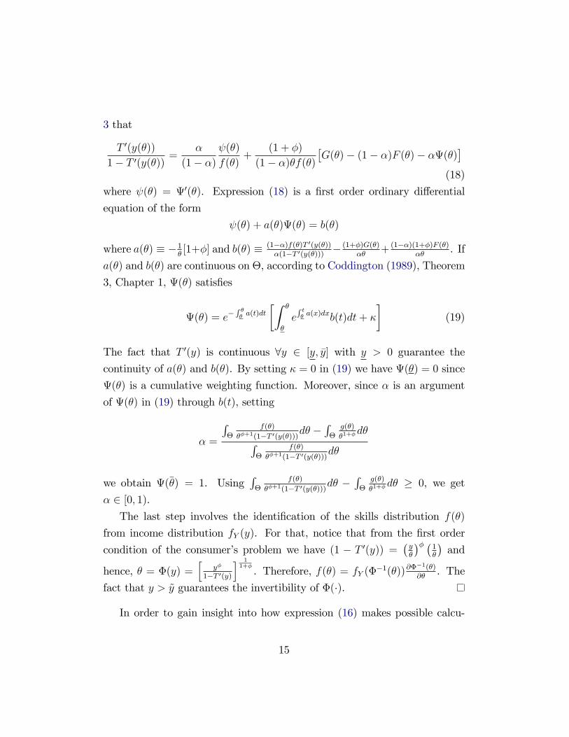
where (�) = 0(�). Expression (18) is a �rst order ordinary di¤erential

equation of the form

(�) + a(�)(�) = b(�)

where a(�) � �1�[1+�] and b(�) � (1��)f(�)T 0(y(�))

�(1�T 0(y(�))) �(1+�)G(�)

��+ (1��)(1+�)F (�)

��. If

a(�) and b(�) are continuous on �, according to Coddington (1989), Theorem

3, Chapter 1, (�) satis�es

(�) = e�R �� a(t)dt

�Z �

�

eR t� a(x)dxb(t)dt+ �

�(19)

The fact that T 0(y) is continuous 8y 2 [y; �y] with y > 0 guarantee the

continuity of a(�) and b(�). By setting � = 0 in (19) we have (�) = 0 since

(�) is a cumulative weighting function. Moreover, since � is an argument

of (�) in (19) through b(t), setting

� =

R�

f(�)

��+1(1�T 0(y(�)))d� �R�

g(�)

�1+�d�R

�f(�)

��+1(1�T 0(y(�)))d�

we obtain (��) = 1. UsingR�

f(�)

��+1(1�T 0(y(�)))d� �R�

g(�)

�1+�d� � 0, we get

� 2 [0; 1).The last step involves the identi�cation of the skills distribution f(�)

from income distribution fY (y). For that, notice that from the �rst order

condition of the consumer�s problem we have (1 � T 0(y)) =�y�

�� �1�

�and

hence, � = �(y) =h

y�

1�T 0(y)

i 11+�. Therefore, f(�) = fY (�

�1(�))@��1(�)@�

. The

fact that y > ~y guarantees the invertibility of �(�).

In order to gain insight into how expression (16) makes possible calcu-

15

lating the jealousy parameter, �, let us consider a very simple example.

Suppose that g(�) = f(�)8� 2 �. Thus, we are in a case of distributionalindi¤erence and as established before, the observed marginal tax T 0(y(�))

must be purely Pigouvian (see equation (13)). Further, let us assume that

T 0(y(�)) = T 08y 2 [y; �y], i.e., society faces a �at tax. Evaluating equation(16), we obtain � = T 0. Thus, we recover the jealousy parameter from taxes.

We can then proceed to calculate (�), the externality weighting function,

using equation (14).

2.6 An Upper Bound for the Jealousy Parameter and

a Lower Bound for the Externality at the Top

As stated in Theorem 1, it is possible to calculate (�) and � conditional on

the redistributive taste of the planner represented by the density g(�). This

element, however, is non observable and thus the model I present has an iden-

ti�cation problem. Nevertheless, it is possible to calculate an upper bound of

� under the loose assumption that society favors some redistribution. This

statement is formally expressed in Proposition 4.

Proposition 4. Let �F � fg : � ! R+ j G(�) � F (�) 8� 2 �g. Then� � �� 8g 2 �F , where � satis�es (16) and

�� =

R�

f(�)T 0(y(�))

�1+�(1�T 0(y(�)))d�R�

f(�)

�1+�(1�T 0(y(�)))d�=EY [y

��T 0(y)]

EY [y��]

Moreover,

f(�) = argmaxg(�)f� j g 2 �Fg

Proof. See Appendix C.

Proposition 5. Suppose T 0(y(��)) � T 0(y(�))8� 2 � with strict inequality

for some interval I � [a; b] � �; with a � �, b < � then (��)

f(��)> 1 8g 2 �F .

16

Proof. See Appendix C.

Two things need to be highlighted about Proposition 4. First, the calcu-

lation of the upper bound of the jealousy parameter � requires only observed

variables: the labor earnings distribution, the marginal tax schedule on la-

bor income and the elasticity of labor supply. Second, the upper bound

of the jealousy parameter is attained when the planner is utilitarian, i.e.

g(�) = f(�)8� 2 �. The intuition for this result is straightforward: whenthe planner is utilitarian, there is complete distributional indi¤erence (given

the quasi-linearity in preferences) and the Mirrleesian tax is zero at any in-

come level. Thus, all taxation must be Pigouvian. Moreover, under the

assumption that societies redistribute, Proposition 5 �nds a lower bound for

the contribution to the consumption externality at the top of the income dis-

tribution, the ratio (��)

f(��). In other words, the weight by which the agent at the

top of the earnings distribution contributes to the consumption externality

must be strictly greater than one if observed income taxes are thought to be

optimal, partly due to corrective considerations. This implies that the aver-

age consumption may not be an accurate approximation of the consumption

reference point a society faces but rather a weighted average where the top

is weighted more. In the next section, I estimate the upper bound of the

jealousy parameter, �, and the corresponding externality weighting function

(�) for the U.S. and the U.K.

3 The Data

My numerical analysis was done for the U.S. and the U.K. This choice was

based on the public availability of micro-�le tax data that I describe in this

section. For the U.S, I use the Statistics of Income (SOI) Public Use Tax

�les elaborated by the Internal Revenue Service (IRS) and distributed by

the NBER.14 The data consists of the information that U.S. citizens and14See Internal-Revenue-Service (1995-2004).

17

residents submit to the IRS through the 1040, 1040A and 1040EZ tax forms.

Cross-section samples of approximately 100,000 to 150,000 observations are

available for each year from 1960 to 2004. Such samples were designed to

make national level estimates by including a weighting variable to make up

for the strati�ed nature of the sample.15 In order to abstract from capital

holdings, the de�nition of gross income that I use is salaries and wages. This

is the entry of the 1040 tax forms speci�ed as �Wages, salaries, tips, etc�. In

addition, I use the the marginal income tax corresponding to di¤erent income

brackets as a proxy of the labor tax schedule. The marginal income tax was

collected from the �Tax Rate Schedule�from 1995 to 2004 published by the

IRS.

For the U.K, I use the Survey of Personal Incomes (SPI) Public Use File

from the Economic and Social Data Service provided by the University of

Essex.16 These �les are compiled by Her Majesty�s Revenue and Customs:

Knowledge, Analysis & Intelligence, and are based on information held by

HM Revenue and Customs (HMRC) tax o¢ ces on individuals who could

be liable for U.K. taxes. Cross-section samples of approximately 450,000

observations are available for each year from 1995 to 2004.17 The data set

also contains a variable that allows to obtain �gures for the whole U.K.

population. I use the variable de�ned as pay that stands for before taxes

pay from employment net of bene�ts and foreign earnings. Marginal income

taxes are collected from the �Survey of Personal Incomes Public Use Tape

Documentation: Annex D: Rates of Income Tax: 1990-91 to 2004-05" located

in HM-Revenue-&-Customs (1998-2007). This is the variable that I use as a

15The General Description Booklet for the Public Use Tax Files (several years) indicatesthat the sample design is a strati�ed probability sample and the population of tax returnis classi�ed into sub-populations (strata). According to the same source, independentsamples are selected independently from each stratum. A weighting variable is obtainedby dividing the population count of returns in a stratum by the number of sample returnsfor that stratum.16See HM-Revenue-&-Customs (1998-2007).17There is an extra �le for the �scal year 1985-1986. Moreover, the HM Revenue and

Customs: Knowledge, Analysis & Intelligence recently released the �le for 2005.

18

proxy of the labor tax schedule for the U.K.

3.1 Estimation of Gross Labor Income Densities

The period of analysis is 1995-2004 since I have comparable data for the two

countries during these years. Even though the model is static, taking into

account the gross income distributions over several years allows me to obtain

a more �robust�distribution for each country calculated as

fY (y) =1

10

2004Xt=1995

fY;t(y) (20)

To calculate fY;t(y) for t = 1995; :::; 2004, I selected the domain y > $100

measured in 2004 dollars. I calculated fY;t(y) using a gaussian kernel over

many points unequally separated, locating more points at the bottom of the

domain than at the top. This was done in order to obtain more accurate es-

timates from numerical integration while at the same time keeping moderate

the number of grid points.18 Income observations were weighted to obtain

population estimates.

Since income observations are more sparse as income is higher, I smoothed

the data after transforming it into a logarithmic scale. According to Wand,

Marron, and Ruppert (1991), this transformation is appropriate under the

presence of a global width parameter h and data being more sparse at the

top than at the bottom of its domain. Without this transformation, either

the data at the bottom of the distribution would be over-smoothed or the

tail would exhibit spurious bumps. The smoothing window or width for the

U.S. was set at h = 0:9� s:d:�n�1=5, where n is the number of observationsand s:d: is the standard deviation of log(yi), for i = 1; :::; n.19 Silverman18For both countries, the number of grid points was 5,000. Moreover, I also performed

my calculations using alternative kernel functions such as the Epanechnikov and Triangularand results were almost identical. The latter was not surprising given the sample size. SeeSilverman (1986). I use the trapezoid method for the numerical integration.19Indeed, the formula suggested by Silverman (1986) is width = 0:9�A�n�1=5, where

19

50k 100k 150k 200k 250k0

0.5

1

1.5

2

2.5

3

3.5

4x 10

­5

y (2004 dollars)

dens

ity

USUK

5M 10M 15M 20M0

1

2

3

4

5

6x 10

­11

y (2004 dollars)

dens

ity

USUK

Figure 1: Gross Labor Income Distribution in the U.S. and the U.K. 1995-2004

(1986) indicates that such a choice of width performs very well in terms of

mean integrated squared error for a wide range of densities. For the U.K.,

I set h = 2 � s:d: � n�1=5 since lower widths produced a bump at the top

of the distribution.20 Figure 1 shows the estimated densities. I follow the

convention to abbreviate 1000 dollars as k and a million dollars as M.

A = minfs:d:; iqr=1:34g, where iqr stands for interquartile range. For both countries andall years, s:d: was lower than iqr=1:34.20For the U.K., I �rst used Silverman (1986) optimal bandwidth. However, the resulting

income density appeared to need further smoothing at the upper tail. To correct for this,I increased the bandwidth sequentially until the income density looked smooth. Thisexplains the use of h = 2� s:d:� n�1=5.

20

3.2 Estimation of Marginal Income Tax Schedules

For both countries, the marginal income tax that I use is the statutory one.

I use them as a proxy of the respective marginal labor tax schedule. For

the U.S., I collect the tax rates corresponding to di¤erent income brackets

as published by the IRS in the �Tax Rate Schedule� from 1995 to 2004. I

use the brackets corresponding to single people. To come up with a single

marginal tax rate schedule for several years, I express all tax rate schedules

in 2004 dollars and for every y, I take a simple average over the ten years

I collected data. To maintain the constructed tax rate as a step function,

I de�ne the boundaries of the brackets as the average boundary of yearly

brackets. For the U.K., I employ exactly the same procedure. This time,

I collect statutory income tax rates from the �Survey of Personal Incomes

Public Use Tape Documentation: Annex D: Rates of Income Tax: 1990-91

to 2004-05" located in HM-Revenue-&-Customs (1998-2007). Figure 2 shows

the estimated marginal income tax schedules.

4 Results

In this section, I present my estimates of agents� jealousy parameter, �,

and their contribution to the consumption externality, the ratio (�)f(�) .

21 This

is done for the case in which the benevolent planner is utilitarian, i.e.,

g(�) = f(�)8� 2 �. In this instance, all taxation is Pigouvian or correctiveand the jealousy parameter attains its upper bound as shown in Proposition

4. That is, � = ��. Under the assumption that the American and British

societies redistribute, the jealousy parameter, �; associated with the �ac-

tual�planner�s weighting density will not be higher than ��. The estimated

parameters are surprisingly moderate. For the American society, I estimate

��us = 0:135 while for the British one, I obtain ��uk = 0:14. Thus, under the

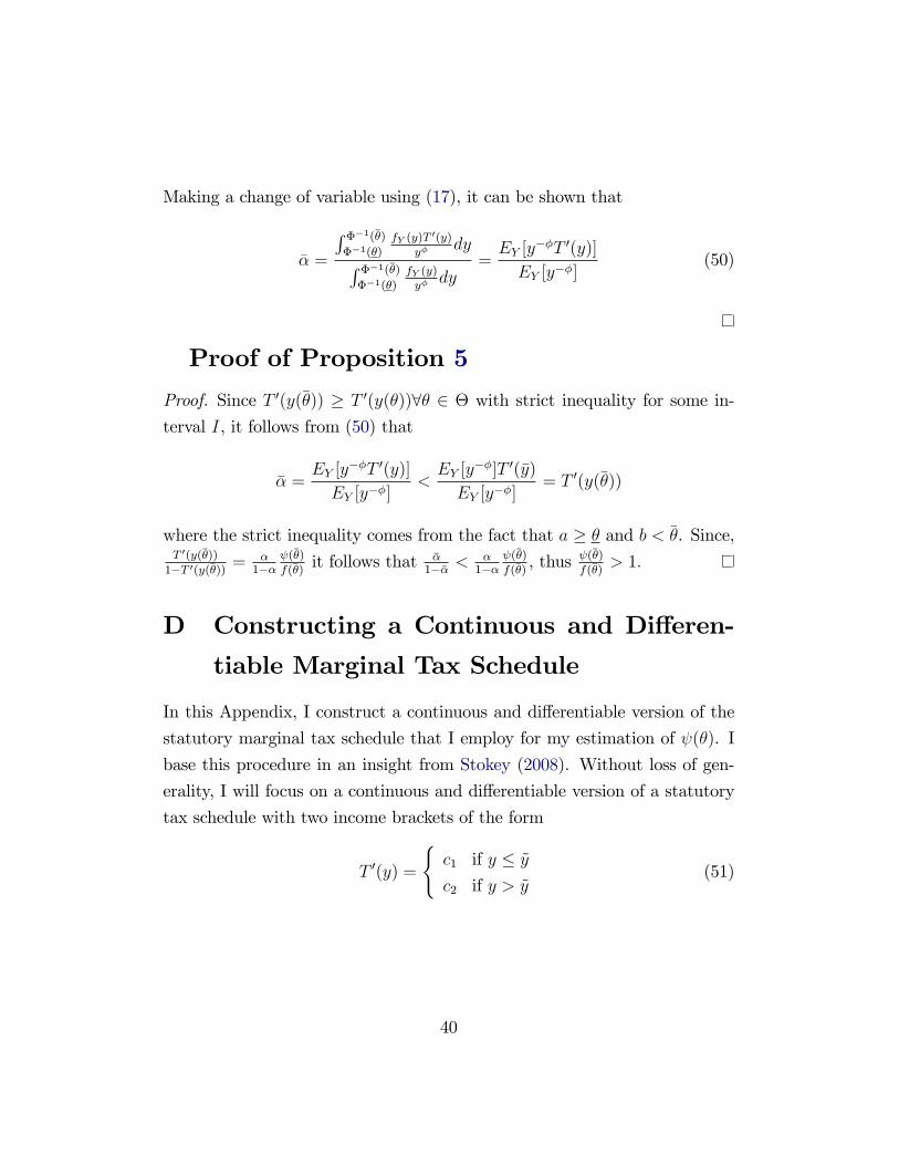
21The estimation uses a continuous and di¤erentiable version of the marginal tax sched-ule. See Appendix D for details.

21

0 50k 100k 150k 200k 250k 300k 350k 400k0

0.1

0.2

0.3

0.4

0.5

0.6

y (2004 dollars)

Tax 

rate

USUK

Figure 2: Statutory Marginal Income Tax in the U.S. and the U.K. 1995-2004

22

assumption that the respective planner is utilitarian, both societies seems to

have very similar positional concerns.

A more intuitive interpretation of the above numbers is the following: an

individual in the U.S. (U.K.) is at least as well o¤ between consuming what

she can purchase with one dollar (pound) than seeing the consumption of

others fall by what they can buy with 13.5 cents (14 pence). Alternatively,

if all agents in the U.S. (U.K.) were given one unit of the consumption good,

from the point of view of a given agent such a consumption would taste at

least like 0.865 (0.86) units after realizing that not only her but all agents

increased their consumption.

Now, the question is, what is the consumption externality contribution

by income in these economies? To answer this, I plot (�)f(�) against the gross

income cdf, FY (y). I present my estimations under the assumption that

the planner is utilitarian and that � = 3 for both countries.22 That is,

the elasticity of labor supply is 13. This choice is in line with the work of

Diamond (1998) who chooses � = f2; 5g for a model with no income e¤ectsand constant elasticity of labor supply.23

According to Figure 3, the ratio (y)f(y)

is, roughly speaking, increasing in

income for both countries. In other words, the contribution to the consump-

tion externality is higher the more a­ uent individuals are.24 More precisely,

the ratio (y)f(y)

in the United Kingdom is almost �at and close to 1.75 from the

third decile to the 85th percentile of the gross earnings distribution. From

there on, it increases sharply reaching a level close to 4. For the United

States, this ratio is close to one up to the 5th decile of the gross earnings

distribution and then increases sharply reaching a level of around 2.5. This

variable exhibits another sharp increase at the very upper tail of the gross

22Evers, Mooij, and Vuuren (2005) �nd that di¤erences in estimates of labor supplyelasticities across countries appear to be small. Both, U.S. and U.K. are included in theirsample of countries.23This choice is based on the work of Pencavel (1986). The results are robust qualita-

tively and quantitatively to elasticities within this range.24This result is in line with one of the �ndings of Blanch�ower and Oswald (2004).

23

0 0.2 0.4 0.6 0.80.5

1

1.5

2

2.5

3

3.5

4

4.5Income values: F(y)≤ 0.99, φ=3

F(y)

ψ(y

)/f(y

)

US, αus=0.135

UK, αuk=0.14

0.99 0.992 0.994 0.996 0.9982

2.5

3

3.5

4

4.5

5Income values: 0.99999>F(y)>0.99,φ=3

F(y)

ψ(y

)/f(y

)

US, αus=0.135

UK, αuk=0.14

Figure 3: Contribution to the Consumption Externality in the U.S. and theU.K. 1995-2004

24

distribution where it hits a level close to 4. Not surprisingly, the ratio (y)f(y)

at the top of the earnings distribution is higher than one as stated in Propo-

sition 5. These estimations suggest that the average consumption may not

be an accurate consumption reference point but rather a weigthed average

where more a­ uent individuals are weighted higher.

5 Conclusions

In this article I have presented a model that rationalizes high labor income

taxes on a­ uent individuals: taxation at the high end of the labor earnings

distribution may occur due to corrective considerations. This happens in

the absence of a non-linear consumption tax schedule. Surprisingly, the esti-

mated parameters that capture what is known in the literature as �jealousy�

for the U.S. and the U.K. are moderate, yet producing quantitatively high

e¤ects over labor income tax rates.

Rationalizing observed labor income taxes as Pigouvian requires that the

consumption externalities exerted by individuals be increasing in income. In

other words, in the light of this model, observed income taxes in the U.S.

and the U.K. are optimal if more a­ uent individuals generate a higher con-

sumption externality than individuals with lower income and the government

corrects this externality.

In future work it is important to analyze, at least numerically, how robust

the results of this paper are once the quasilinearity assumption is abandoned.

It would also be interesting to explore to what extent the presumed higher

contribution of a­ uent consumers to the consumption externality is a result

of these agents having access to consumption goods with higher positional

e¤ects and the government not being able to tax these goods directly.25 This

line of research is currently being explored in Samano (2009). Further re-

25In Frank (2008)�s terminology, a good is positional if its valuation depends highly onthe context.

25

search is also necessary to understand whether positional concerns are purely

instrumental as in Cole, Mailath, and Postlewaite (1992) and Postlewaite

(1998) or �hard-wired� in human beings. The latter is the hypothesis of

Maccheroni, Marinacci, and Rustichini (2009). Finally, as Hopkins (2008)

points out, additional empirical research is needed to examine how the e¤ect

of others� income varies across the income distribution. In this paper, the

parameter that captures this e¤ect has been kept constant across agents.

References

Abel, A. (1990): �Asset prices under habit formation and catching up with

the Joneses,�The American Economic Review, 80(2), 38�42.

(2005): �Optimal Taxation when Consumers Have Endogenous

Benchmark Levels of Consumption,�Review of Economic Studies, 72(1),

21�42.

Alpizar, F., F. Carlsson, and O. Johansson-Stenman (2005): �How

much do we care about absolute versus relative income and consumption?,�

Journal of Economic Behavior and Organization, 56(3), 405�421.

Atkinson, A. (1990): �Public economics and the economic public,�Euro-

pean Economic Review, 34(2-3), 225�248.

Bault, N., G. Coricelli, and A. Rustichini (2008): �Interdependent

utilities: How social ranking a¤ects choice behavior,�PLoS ONE, 3(10).

Blanchflower, D., and A. Oswald (2004): �Well-being over time in

Britain and the USA,�Journal of Public Economics, 88(7-8), 1359�1386.

Boskin, M., and E. Sheshinski (1978): �Optimal redistributive taxation

when individual welfare depends upon relative income,� The Quarterly

Journal of Economics, 94(2), 589�601.

26

Campbell, J., and J. Cochrane (1999): �By force of habit: A

consumption-based explanation of aggregate stock market behavior,�Jour-

nal of Political Economy, 107(2), 205�251.

Carlsson, F., O. Johansson-Stenman, and P. Martinsson (2007):

�Do You Enjoy Having More than Others? Survey Evidence of Positional

Goods,�Economica, 74(4).

Clark, A., and A. Oswald (1996): �Satisfaction and comparison income,�

Journal of Public Economics, 61(3), 359�381.

Clark, A., and C. Senik (2008): �Who compares to whom? The anatomy

of income comparisons in Europe,� Working Paper 65, Paris School of

Economics.

Coddington, E. (1989): An Introduction to Ordinary Di¤erential Equa-

tions. Courier Dover Publications.

Cole, H., G. Mailath, and A. Postlewaite (1992): �Social Norms,

Savings Behavior, and Growth,� Journal of Political Economy, 100(6),

1092.

Constantinides, G. (1990): �Habit Formation: A Resolution of the Equity

Premium Puzzle,�Journal of Political Economy, 98(3), 519.

Diamond, P. (1998): �Optimal Income Taxation: An Example with a U-

Shaped Pattern of Optimal Marginal Tax Rates,� American Economic

Review, 88(1), 83�95.

Duesenberry, J. (1949): Income, Saving, and the Theory of Consumer

Behavior. Harvard University Press.

Dupor, B., and W. Liu (2003): �Jealousy and Equilibrium Overconsump-

tion,�American Economic Review, 93(1), 423�428.

27

Dynan, K., and E. Ravina (2007): �Increasing income inequality, external

habits, and self-reported happiness,�American Economic Review, 97(2),

226�231.

Evers, M., R. Mooij, and D. Vuuren (2005): �What Explains the Vari-

ation in Estimates of Labour Supply Elasticities?,�CESifo Working Paper

1633.

Ferrer-i Carbonell, A. (2005): �Income and well-being: an empirical

analysis of the comparison income e¤ect,� Journal of Public Economics,

89(5-6), 997�1019.

Frank, R. (2008): �Should public policy respond to positional externali-

ties?,�Journal of Public Economics, 92(8), 1777�1786.

Gali, J. (1994): �Keeping up with the Joneses: Consumption Externali-

ties, Portfolio Choice, and Asset Prices,� Journal of Money, Credit and

Banking, 26(1), 1�8.

Heaton, J. (1995): �An empirical investigation of asset pricing with tempo-

rally dependent preference speci�cations,�Econometrica, 63(3), 681�717.

HM-Revenue-&-Customs (1998-2007): Survey of Personal Incomes, Sev-

eral Years: Public Use Tape [computer �le]. Colchester, Essex: UK Data

Archive [distributor].

Hopkins, E. (2008): �Inequality, happiness and relative concerns: What

actually is their relationship?,�Journal of Economic Inequality, 6(4), 351�

372.

Internal-Revenue-Service (1995-2004): Statistics of Income: Individual

Tax Returns. Washington, D.C: U.S. Government Printing O¢ ce.

Ireland, N. (2001): �Optimal income tax in the presence of status e¤ects,�

Journal of Public Economics, 81(2), 193�212.

28

J. Solnick, S., and D. Hemenway (1998): �Is more always better?: A

survey on positional concerns,�Journal of Economic Behavior and Orga-

nization, 37(3), 373�383.

Ljungqvist, L., and H. Uhlig (2000): �Tax Policy and Aggregate De-

mand Management Under Catching Up with the Joneses,�American Eco-

nomic Review, 90(3), 356�366.

Luttmer, E. (2005): �Neighbors as Negatives: Relative Earnings and Well-

Being,�The Quarterly Journal of Economics, 120(3), 963�1002.

Maccheroni, F., M. Marinacci, and A. Rustichini (2009): �Social De-

cision Theory: Choosing within and between Groups,�Mimeo, Universita

Bocconi, Collegio Carlo Alberto and University of Minnesota.

McBride, M. (2001): �Relative-income e¤ects on subjective well-being in

the cross-section,�Journal of Economic Behavior and Organization, 45(3),

251�278.

Mirrlees, J. (1971): �An Exploration in the Theory of Optimum Income

Taxation,�Review of Economic Studies, 38(114), 175�208.

Neumark, D., and A. Postlewaite (1998): �Relative income concerns

and the rise in married women�s employment,� Journal of Public Eco-

nomics, 70(1), 157�183.

Oswald, A. (1983): �Altruism, jealousy and the theory of optimal non-

linear taxation,�Journal of Public Economics, 20(1), 77�87.

Pencavel, J. (1986): �Labor Supply of Men: A Survey,�Handbook of Labor

Economics, 1, 3�102.

Postlewaite, A. (1998): �The social basis of interdependent preferences,�

European Economic Review, 42(3-5), 779�800.

29

Rustichini, A., and A. Vostroknutov (2007): �Competition with Skill

and Luck,�Mimeo, University of Minnesota.

Sadka, E. (1976): �On income distribution, incentive e¤ects and optimal

income taxation,�Review of Economic Studies, 43(2), 261�8.

Saez, E. (2001): �Using Elasticities to Derive Optimal Income Tax Rates,�

Review of Economic Studies, 68(1), 205�229.

Salanié, B. (1997): The Economics of Contracts: A Primer. MIT Press.

Samano, D. (2009): �Optimal Linear Taxation of Positional Goods,�

Mimeo, University of Minnesota.

Seade, J. (1977): �On the Shape of Optimal Tax Schedules,� Journal of

Public Economics, 7(2), 203�235.

Senik, C. (2008): �Ambition and Jealousy: Income Interactions in the

Old Europe Versus the New Europe and the United States,�Economica,

75(299), 495�513.

Silverman, B. (1986): Density Estimation for Statistics and Data Analysis.

Chapman & Hall/CRC.

Stokey, N. (2008): Economics of Inaction: Stochastic Control Models with

Fixed Costs. Princeton University Press.

Tuomala, M. (1990): Optimal Income Tax and Redistribution. Oxford Uni-

versity Press, USA.

Veblen, T. (1899): The Theory of the Leisure Class, 1934 edition.

Wand, M., J. Marron, and D. Ruppert (1991): �Transformations

in density estimation,� Journal of the American Statistical Association,

86(414), 343�353.

Werning, I. (2007): �Pareto E¢ cient Income Taxation,�Mimeo, MIT.

30

Appendix

A Proofs

Proof of Proposition 1

Proof. The �rst step is to transform the continuum of incentive compatibility

constraints (4) into a �rst order condition. Let

W (�; �0) � u(c(�0); C)� v

�y(�0)

�

�(21)

A necessary condition for truthful revelation of type is @W (�;�0)@�0 j�0=� = 0,

therefore it follows that

uc(c(�); C)c0(�) = v0

�y(�)

�

�y0(�)

�8� 2 � (22)

Moreover, under truthful revelation W (�) = u(c(�); C) � v�y(�)�

�and

hence,W 0(�) = uc(c(�); C)c0(�)�v0

�y(�)�

�y0(�)�+v0

�y(�)�

�y(�)

�2, which together

with (22) becomes

W 0(�) = v0�y(�)

�

�y(�)

�28� 2 �: (23)

FollowingWerning (2007), I de�ne the expenditure function e(W (�); y(�); C; �)

to satisfy W (�) = u(e; C)� v�y(�)�

�. The planner problem can be reestated

as

maxW (�);y(�);C

Z�

W (�)g(�)d� (24)

s.tZ�

e(W (�); y(�); C; �)f(�)d� =

Z�

y(�)f(�)d� (25)

31

W 0(�) = v0�y(�)

�

�y(�)

�28� 2 � (26)

C =

Z�

e(W (�); y(�); C; �) (�)d� (27)

The corresponding Lagrangian is

L(W (�); y(�); C; �; �(�); ) =

Z�

W (�)g(�)d���Z�

[(e(W (�); y(�); C; �)� y(�)) f(�)] d�

+

Z�

�(�)

�W 0(�)� v0

�y(�)

�

�y(�)

�2

�d�+

�C �

Z�

e(W (�); y(�); C; �) (�)d�

�(28)

Using integration by parts, it follows thatZ�

�(�)W 0(�)d� = �(��)W (��)� �(�)W (�)�Z�

�0(�)W (�)d� (29)

thus, we can reexpress the above Lagrangian as

L(W (�); y(�); C; �; �(�); ) =

Z�

W (�)g(�)d���Z�

�(e(W (�); y(�); C; �)�y(�))f(�)

�d�

+�(��)W (��)� �(�)W (�)�Z�

�0(�)W (�)d� �Z�

�(�)v0�y(�)

�

�y(�)

�2d�

+

�C �

Z�

e(W (�); y(�); C; �) (�)d�

�(30)

Assuming interior solution, it follows from �rst order conditions that

32

W (�):

g(�)� �f(�)eW (W (�); y(�); C; �)� �0(�)� (�)eW (W (�); y(�); C; �) = 0

(31)

y(�):

��ey(W (�); y(�); C; �)f(�) + �f(�)� �(�)

�2v0�y(�)

�

��1 +

1

�(�)

�

� ey(W (�); y(�); C; �) (�) = 0 (32)

C :

��Z�

eC(W (�); y(�); C; �)f(�)d� + �

Z�

eC(W (�); y(�); C; �) (�)d� = 0

(33)

together with the boundary conditions �(�) = �(��) = 0 and where �(�) �v0( y(�)

�)

v00( y(�)�)y(�)�

. Moreover, implicitly di¤erentiating W (�) = u(e; C)� v�y(�)�

�we

have that eW (W (�); y(�); C; �) = 1uc(c(�);C)

, ey(W (�); y(�); C; �) =v0( y(�)� )

1�

uc(c(�);C)

and eC(W (�); y(�); C; �) = �uC(c(�);C)uc(c(�);C)

. The result follows after manipulating

(31)-(33).

Proof of Proposition 2

Proof. Taking �rst order conditions in agent�s problem we have

T 0(y(�))

1� T 0(y(�))=uc(c

eq(�); Ceq)

v0�yeq(�)�

�1�

� 1 (34)

where Ceq =R�ceq(�) (�)d�. Substituting (11) into (34) it follows that

uc(ceq(�)); Ceq)

v0(yeq(�)�)1�

� 1 = (�)

�f(�)+

33

uc(c�(�); C�)

�f(�)

�1 +

1

��(�)

� Z �

�

�g(t)

�� f(t)

uc(c�(t); C�)�

�

(t)

uc(c�(t); C�)

�dt

(35)

Since in equilibrium the government balances its budget, we must have

that Z�

ceq(�)f(�)d� =

Z�

yeq(�)f(�)d� (36)

thus from (35)-(36) we conclude that fceq(�); yeq(�)g�2� = fc�(�); y�(�)g�2�.

Proof of Proposition 3

Proof. By quasi-linearity of preferences uc(c(�); C) = 1. Thus, using expres-

sion (11), the optimal income tax satis�es

T 0(y�(�))

1� T 0(y�(�))=

�

(�)

f(�)+

1

�f(�)

�1 +

1

��(�)

��(�)

�(37)

with

�(�) =

Z �

�

[g(t)� �f(t)� (t)]dt: (38)

By boundary conditions we have �(��) = 0, henceZ�

[g(t)� �f(t)� (t)]dt = 0 ) � = 1� (39)

which together with the fact that �= �

1�� which follows from expression

(7) when preferences are quasi-linear implies that � = 1 � � and = �.

Plugging the previous values into (37) and substituting into (38) delivers the

result after algebraic manipulations.

34

B Asymptotic Tax in a Quasi-Linear Envi-

ronment

Under the assumption that �� < 1 it can be seen from Corollary 1 thatT 0(y�(��))1�T 0(y�(��)) =

�(1��)

(��)

f(��). Hence, under a bounded distribution of skills I obtain

a non-zero taxation at the top due to corrective considerations. Proposition

6 exhibits the formula for the optimal marginal labor income tax as �� goes to

in�nity. I consider the case of quasi-linear preferences, a constant elasticity

of labor supply and f(�) Pareto-distributed. The last assumption is used

based on Diamond (1998) and Saez (2001). Both studies obtain positive

asymptotic marginal tax rates, however these results depend critically on

f(�) being Pareto.26

Proposition 6. Suppose f(�) is Pareto distributed with parameter k > 0 andthat L1 � lim�!1

(�)f(�)

and L2 � lim�!1g(�)f(�)

exist. If u(c(�); C) = c(�) ��C, � 2 [0; 1), v

�y�

�= 1

1+�

�y�

�1+�; � > 0 then T 01

1�T 01= �

(1��)L1�1+�+k

k

�+

1+�k

h1� 1

(1��)L2

iwhere T 01 � lim�!1 T

0(y�(�)).

Proof. From Proposition (3) and simple algebraic manipulations we have

T 0(y�(�))

1� T 0(y�(�))=

�

(1� �)

(�)

f(�)+

1� F (�)

(1� �)�f(�)

�1 +

1

��(�)

��

[G(�)� (1� �)F (�)� �(�)]

1� F (�)(40)

Since f(�) is Pareto it follows that 1�F (�)�f(�)

= 1kand since v(y

�) = 1

1+�

�y�

�1+�we have that

h1 + 1

��(�)

i= 1+ �. Using the fact that L1 � lim�!1

(�)f(�)

<1

26For a Pareto distribution f(�) = k�k

�k+1; � 2 [�;1); � > 0; k > 0 and F (�) = 1�

���

�k.

35

it follows that

lim�!1

T 0(y�(�))

1� T 0(y�(�))=

�

1� �L1+

(1 + �)

k(1� �)lim�!1

�G(�)� (1� �)F (�)� �(�)

�1� F (�)

(41)

Using L�Hôpital�s rule, lim�!1

�G(�)�(1��)F (�)��(�)

�1�F (�) = �L2 + (1� �) + �L1

and substituting into (41) delivers the result.

Corollary 2 (Proposition 3). If L1 � 1 and L2 � 1, then T 01 � �.

Proof. Trivial.

Figure 4 shows the ratio 1�FY (y)yfY (y)

of the income distribution in the U.S. for

1992, 1993 and from 1995-2004. I include the years 1992 and 1993 since Saez

(2001) estimates a Pareto distribution parameter for labor earnings based

on these years. This ratio was constructed after smoothing the upper tail of

fY (y) using a gaussian kernel. The width was set at h = 1:36� s:d:� n�1=5,where the standard deviation (s:d:) and n were calculated for observations

exceeding 13.5 million dollars (expressed in 2004 dollars). Table 1 reports

the number of observations, n, in the sample exceeding that threshold.27

Table 1: In Sample Number of Gross Income ObservationsExceeding $13,500,000 (2004 dollars)

Year Observations Year Observations1992 153 1999 4861993 75 2000 6661995 78 2001 4051996 134 2002 2611997 217 2003 2821998 333 2004 391

It can be seen that at least for some years the ratio 1�FY (y)yfY (y)

at the very top

of the distribution is decreasing. This fact indicates that the very top of the27This amount is approximately equivalent to 10 million expressed in 1992 dollars. Saez

(2001) reports that starting at this income level the number of taxpayers in the databaseis very small.

36

income distribution of the United States may not be accurately represented

by a Pareto distribution. Moreover, a decreasing 1�FY (y)yfY (y)

would imply a de-

creasing pattern of optimal taxes in the canonical Mirrleesian model. This is

indeed what Mirrlees (1971) �nds since he assumes a log-normal distribution

of skills for which the ratio is decreasing. The model with consumption ex-

ternalities would deliver asymptotic non-zero optimal taxes even if the ratio1�FY (y)yfY (y)

is decreasing.

C Proof of Proposition 4

Proof. Observe that we can reexpress (16) as28

� =

R�

f(�)T 0(y(�))

�1+�(1�T 0(y(�)))d� + (1 + �)R�(F (�)�G(�))

�2+�d�R

�f(�)T 0(y(�))

�1+�(1�T 0(y(�)))d� + (1 + �)R�F (�)

�2+�d� + 1

��1+�

(45)

Thus,

�� = maxG(�)

f� j G(�) � F (�) 8� 2 �; G0(�) � 0; G(�) = 0; G(��) = 1g

28 To see this, observe thatZ�

f(�)

�1+�(1� T 0(y(�)))d� =

Z�

f(�)T 0(y(�))

�1+�(1� T 0(y(�)))d� +

Z�

f(�)

�1+�d� (42)

Using integration by parts it follows that

(1 + �)

Z�

F (�)

��+2d� = � 1

��1+�

+

Z�

f(�)

�1+�d� (43)

Plugging (43) into (42) we obtain that the denominator of (45) is equal to the denominatorof (16). To see that the numerator of (45) is equal to the one in (16) use expression (42)together with the fact that by integration by partsZ

�

g(�)

�1+�d� = (1 + �)

Z�

G(�)

��+2d� +

1

��1+�

(44)

37

2 4 6 8 10 12

x 107

0

0.2

0.4

0.6

0.8

1

y (2004 dollars)

2004

5 10 15

x 107

0

0.2

0.4

0.6

0.8

1

y (2004 dollars)

2003

2 4 6 8

x 107

0

0.2

0.4

0.6

0.8

1

y (2004 dollars)

2002

2 4 6 8 10 12 14

x 107

0

0.2

0.4

0.6

0.8

1

y (2004 dollars)

2001

2 4 6 8 10 12

x 107

0

0.2

0.4

0.6

0.8

1

y (2004 dollars)

2000

2 4 6 8 10 12 14

x 107

0

0.2

0.4

0.6

0.8

1

y (2004 dollars)

1999

2 4 6 8 10 12 14

x 107

0

0.2

0.4

0.6

0.8

1

y (2004 dollars)

1998

2 4 6 8 10 12

x 107

0

0.2

0.4

0.6

0.8

1

y (2004 dollars)

1997

2 4 6

x 107

0

0.2

0.4

0.6

0.8

1

y (2004 dollars)

1996

2 3 4 5

x 107

0

0.2

0.4

0.6

0.8

1

y (2004 dollars)

1995

5 10 15

x 107

0

0.5

1

1.5

y (2004 dollars)

1993

2 4 6 8 10 12 14

x 107

0

0.2

0.4

0.6

0.8

1

y (2004 dollars)

1992

Figure 4: Kernel smoothed 1�FY (y)yfY (y)

ratio in the U.S. y � $13; 500; 000(2004 dollars)

38

To obtain G(�), I solve the following maximization problem

maxG(�)

Z�

(F (�)�G(�))

�2+�d�

s.t.

G(�) � F (�)8� 2 � (46)

G0(�) � 0; G(�) = 0; G(��) = 1 (47)

Let me consider the optimization problem ignoring constraints (47). The

corresponding Lagrangian is

L(G(�); (�);F (�); �) =

Z�

(F (�)�G(�))

�2+�d� +

Z�

(�)[G(�)� F (�)]d�

The �rst order condition with respect to G(�) is

1

�2+�= (�) 8� 2 � (48)

Clearly, (�) > 08� 2 �. By the slackness condition, we must have

(�)[G(�)� F (�)] = 0 8� 2 � (49)

thus, G(�) = F (�)8� 2 �. Clearly this solution satis�es (47). Finally,

substituting g(�) = f(�) into (16) we obtain

�� =

R�

f(�)T 0(y(�))

�1+�(1�T 0(y(�)))d�R�

f(�)

�1+�(1�T 0(y(�)))d�:

39

Making a change of variable using (17), it can be shown that

�� =

R ��1(��)��1(�)

fY (y)T0(y)

y�dyR ��1(��)

��1(�)fY (y)y�

dy=EY [y

��T 0(y)]

EY [y��](50)

Proof of Proposition 5

Proof. Since T 0(y(��)) � T 0(y(�))8� 2 � with strict inequality for some in-

terval I, it follows from (50) that

�� =EY [y

��T 0(y)]

EY [y��]<EY [y

��]T 0(�y)

EY [y��]= T 0(y(��))

where the strict inequality comes from the fact that a � � and b < ��. Since,T 0(y(��))1�T 0(y(��)) =

�1��

(��)

f(��)it follows that ��

1��� <�1��

(��)

f(��), thus (��)

f(��)> 1:

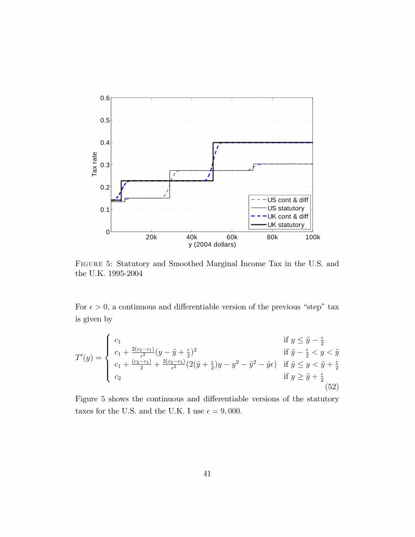
D Constructing a Continuous and Di¤eren-

tiable Marginal Tax Schedule

In this Appendix, I construct a continuous and di¤erentiable version of the

statutory marginal tax schedule that I employ for my estimation of (�). I

base this procedure in an insight from Stokey (2008). Without loss of gen-

erality, I will focus on a continuous and di¤erentiable version of a statutory

tax schedule with two income brackets of the form

T 0(y) =

(c1 if y � ~yc2 if y > ~y

(51)

40

20k 40k 60k 80k 100k0

0.1

0.2

0.3

0.4

0.5

0.6

y (2004 dollars)

Tax 

rate

US cont & diffUS statutoryUK cont & diffUK statutory

Figure 5: Statutory and Smoothed Marginal Income Tax in the U.S. andthe U.K. 1995-2004

For � > 0, a continuous and di¤erentiable version of the previous �step�tax

is given by

T 0(y) =

8>>>><>>>>:c1 if y � ~y � �

2

c1 +2(c2�c1)

�2(y � ~y + �

2)2 if ~y � �

2< y < ~y

c1 +(c2�c1)

2+ 2(c2�c1)

�2(2(~y + �

2)y � y2 � ~y2 � ~y�) if ~y � y < ~y + �

2

c2 if y � ~y + �2

(52)

Figure 5 shows the continuous and di¤erentiable versions of the statutory

taxes for the U.S. and the U.K. I use � = 9; 000.

41