Preliminary report, presented and distributed on September 30, 2008, at the

8th International Conference on Creep and Shrinkage of Concrete

(CONCREEP-8), held in Ise-Shima, Japan

Revised March 9, 2009 (download from: http://www.civil.northwestern.edu

/people/bazant/PDFs/Papers/PalauCreep-09-03-9.pdf )

Explanation of Excessive Long-Time Deflections ofCollapsed Record-Span Box Girder Bridge in Palau

Zdenek P. Bazant, Guang-Hua Li, Qiang Yu,

Gary Klein and Vladimır Krıstek

Preliminary Structural Engineering ReportNo. 08-09/A222e

Infrastructure Technology InstituteMcCormick School of Engineering and Applied Science

Northwestern UniversityEvanston, Illinois 60208, USA

September 19, 2008Updated March 9, 2009

Explanation of Excessive Long-Time Deflections ofCollapsed Record-Span Box Girder Bridge in Palau1

Zdenek P. Bazant2, Guang-Hua Li3, Qiang Yu4, Gary Klein5 and Vladimır Krıstek6

Abstract: Explanation of the excessive deflections of the Koror-Babeldaob (KB) Bridge in Palauis presented. This bridge was built in 1977 by the cantilever method and collapsed 3 months afterremedial prestressing in 1996. It was a segmental prestressed concrete girder having the world-record span of 241 m (790 ft.) and maximum girder depth of 14.17 m (46.5 ft). The final mid-spandeflection was in design expected to be 0.55 to 0.67 m (21.6 to 26.4 in), but after 18 years itreached 1.39 m (54.6 in.) and was still growing. Presented is a comprehensive analysis using 5906three-dimensional (3D) finite elements and step-by-step integration in time. For the concrete creepand shrinkage properties, the B3, GL, ACI and CEB (or CEB-FIP, fib) models are considered andpredictions compared. Model B3, in contrast to the others, does not give an unambiguous predictionbecause, in addition to concrete design strength, it necessitates further input parameters which areunknown. These are three mix parameters which can be set to default values but can also be variedover a realistic range to ascertain the range of realistic predictions. The findings are as follows: 1) Formodel B3, one can find plausible values of input parameters for which all the measured deflections(as well as Troxell et al.’s 23-year creep tests) can be closely matched, while for the other modelsthey cannot even be approached and the observed shape of creep curve cannot be reproduced. 2)The 19-year deflections calculated by 3D finite elements according the ACI, CEB and GL modelsare about 67%, 62% and 54% less, respectively, than those measured and calculated according tomodel B3, and their deflection curves have shapes rather different from the those measured. 3)The shear lag is important since it increases the downward deflection due to self-weight much morethan the upward deflection due to prestress. 4) The deflection is highly sensitive to prestress lossbecause it represents a small difference of two large numbers (deflections due to self-weight, and toprestress). According to the ACI, CEB and GL models, the prestress loss obtained by the same finiteelement code is, respectively, about 54%, 44% and 34% smaller, and according to the classical lumpestimate used in design about 54% smaller. 5) Model B3 is in agreement with the measurementsif 3D finite elements with step-by-step time integration are used to calculate both the deflectionsand the prestress losses, and if the differences in shrinkage and drying creep properties caused bydifferences in slab thickness and temperature are taken into account.

Introduction

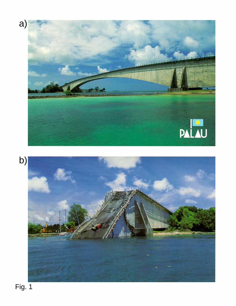
The Koror-Babeldaob (KB) Bridge connected the islands of Koror and Babeldaob in the Re-public of Palau in tropical Western Pacific (Fig. 1a). When completed in 1977, the 241 m (790

1March 2009 revision of September 2008 original version, prepared after additional data were obtained andmore accurate calculations were completed. Also, Appendix III on Japanese bridges is added

2McCormick Institute Professor and W.P. Murphy Professor of Civil Engineering and Materi-als Science, Northwestern University, 2145 Sheridan Road, CEE/A135, Evanston, Illinois 60208; z-bazant@northwestern.edu.

3Graduate Research Assistant and Doctoral Candidate, Northwestern University.4Post-doctoral Research Associate, Northwestern University.5Principal, Wiss, Janey, Elstner, Inc., 330 Pfingsten Rd., Northbrook, Illinois 60062-2095.6Professor, Faculty of Civil Engineering, Czech Technical University in Prague, Czech Republic.

1

ft.) main span set the world record for prestressed concrete box girder bridges [1]. The finaldeflection was expected to terminate at 0.55 to 0.67 m (21.6 to 26.4 in.), according to the orig-inal CEB-FIP design recommendations (1970-72 [2]), which were used in design [3,4]. Accordingto the 1972 ACI model [5], which has been in force until today, the deflection would have beenpredicted as 0.71 m (28 in.) [6]. Unfortunately, after 18 years, the deflection, measured since theend of construction, reached 1.39 m (54.6 in.) and kept growing [3,7]. Compared to the designlevel, the mid-span sag was 0.076 m higher, i.e., 1.47 m because not all of the camber plannedto offset future deflections could be introduced. Remedial prestressing was undertaken, but 3months after its completion (on September 26, 1996) the bridge suddenly collapsed into theToegel channel, with two fatalities (Fig. 1b) [6,8–12].

As a result of legal litigation, the data collected on this major catastrophe by the investigatingagencies have been sealed and unavailable for many years. However, on November 6, 2007, the3rd Structural Engineers’ World Congress in Bangalore endorsed a resolution (proposed by thefirst writer, with the support of many experts). The resolution, which was circulated to majorengineering societies, called, on the grounds of engineering ethics, for the release of all thetechnical data necessary for analyzing major structural collapses, including the bridge in Palau(see Appendix II). Subsequently, the Attorney General of Palau gave his permission.

The objective of this article is to explain the reasons for the excessive long-term deflectionsand draw lessons for the creep and shrinkage analysis of structures. Analysis of the remedialmeasures and the direct causes of collapse is planned for a forthcoming separate article.

Research Significance

Clarification of the causes of major disasters has been, and will always be, the main routeto progress in structural engineering. Understanding of the excessive deflections of the bridgein Palau has the potential of greatly improving the predictions of creep and shrinkage effectsin bridges as well as other structures. It may also help to resolve the currently intractabledisagreements in technical committees about the optimal prediction model for a standard guide.

Bridge Description and Input Data of Analysis

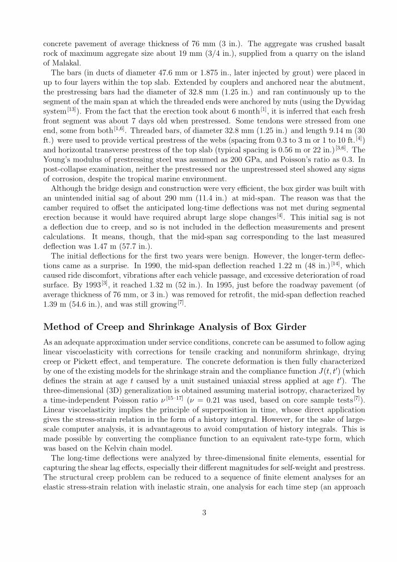
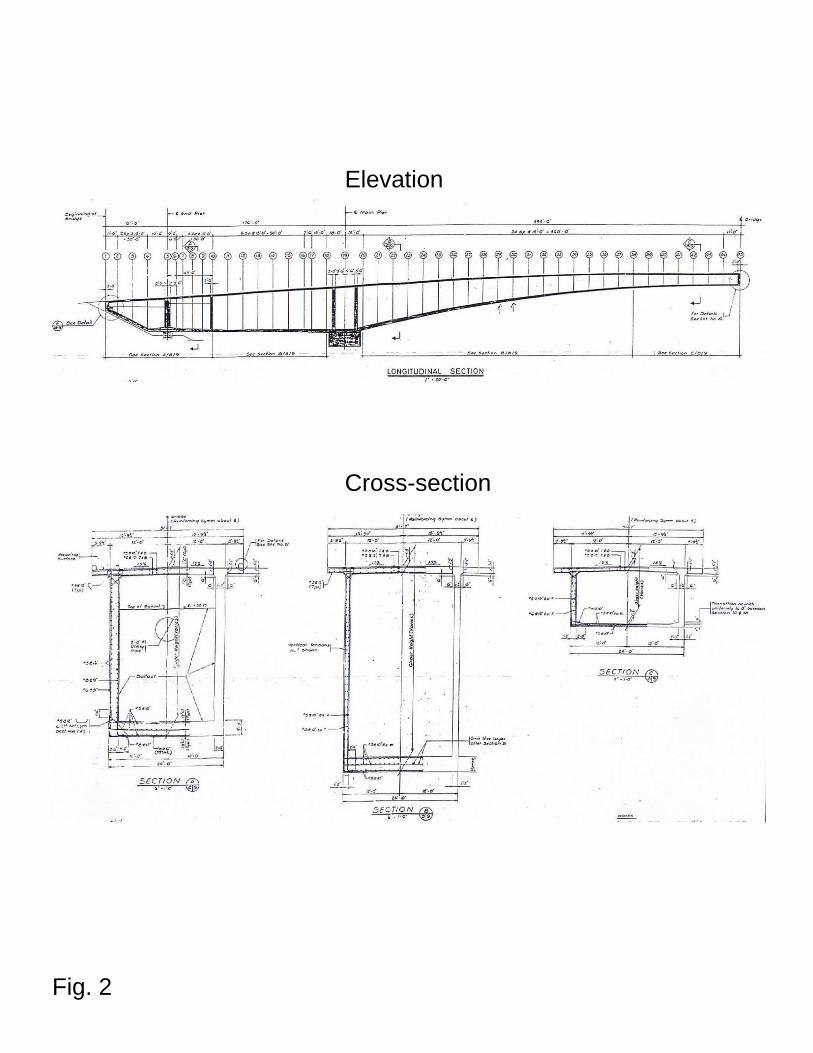
The main span of 241 m (790 ft.) consisted of two symmetric concrete cantilevers connected atmid-span by a horizontally sliding hinge. Each cantilever was made of 25 cast-in-place segmentsof depths varying from 14.17 m (46.5 ft.) at the main piers to 3.66 m (12 ft.) at mid-span.The main span was flanked by 72.2 m (237 ft.) long end spans in which the box girder waspartially filled with rock ballast to balance the moment at the main pier. The total length ofthe bridge was 386 m (1265 ft.). The thickness of the top slab ranged from 432 mm (17 in.) atthe main piers to 280 mm (11 in.) at the mid-span. The thickness of the bottom slab variedfrom 1153 mm (45.4 in.) at the main piers to 178 mm (7 in.) at the mid-span. The webshad an unusually small thickness of 356 mm (14 in.) in the main span. The elevation andseveral typical cross sections are shown in Fig. 2. Both symmetric halves of the bridge wereconstructed simultaneously [1,6]. The whole bridge was completed within 2 years.

According to the design, the initial total longitudinal prestressing force above the main pierwas 211 MN (47,400 kips), and was provided by 316 parallel high-strength threaded bars ofdiameter 32.8 mm (1.25 in.) and strength 1034 MPa (150 ksi) [1,6,10] (the jacking force of eachbar was 135 kips).

The mass density of concrete was ρ = 2325 kg/m3 (144 lb/ft.3) [3]. Top slab was covered by

2

concrete pavement of average thickness of 76 mm (3 in.). The aggregate was crushed basaltrock of maximum aggregate size about 19 mm (3/4 in.), supplied from a quarry on the islandof Malakal.

The bars (in ducts of diameter 47.6 mm or 1.875 in., later injected by grout) were placed inup to four layers within the top slab. Extended by couplers and anchored near the abutment,the prestressing bars had the diameter of 32.8 mm (1.25 in.) and ran continuously up to thesegment of the main span at which the threaded ends were anchored by nuts (using the Dywidagsystem [13]). From the fact that the erection took about 6 month [1], it is inferred that each freshfront segment was about 7 days old when prestressed. Some tendons were stressed from oneend, some from both [1,6]. Threaded bars, of diameter 32.8 mm (1.25 in.) and length 9.14 m (30ft.) were used to provide vertical prestress of the webs (spacing from 0.3 to 3 m or 1 to 10 ft. [4])and horizontal transverse prestress of the top slab (typical spacing is 0.56 m or 22 in.) [3,6]. TheYoung’s modulus of prestressing steel was assumed as 200 GPa, and Poisson’s ratio as 0.3. Inpost-collapse examination, neither the prestressed nor the unprestressed steel showed any signsof corrosion, despite the tropical marine environment.

Although the bridge design and construction were very efficient, the box girder was built withan unintended initial sag of about 290 mm (11.4 in.) at mid-span. The reason was that thecamber required to offset the anticipated long-time deflections was not met during segmentalerection because it would have required abrupt large slope changes [4]. This initial sag is nota deflection due to creep, and so is not included in the deflection measurements and presentcalculations. It means, though, that the mid-span sag corresponding to the last measureddeflection was 1.47 m (57.7 in.).

The initial deflections for the first two years were benign. However, the longer-term deflec-tions came as a surprise. In 1990, the mid-span deflection reached 1.22 m (48 in.) [14], whichcaused ride discomfort, vibrations after each vehicle passage, and excessive deterioration of roadsurface. By 1993 [3], it reached 1.32 m (52 in.). In 1995, just before the roadway pavement (ofaverage thickness of 76 mm, or 3 in.) was removed for retrofit, the mid-span deflection reached1.39 m (54.6 in.), and was still growing [7].

Method of Creep and Shrinkage Analysis of Box Girder

As an adequate approximation under service conditions, concrete can be assumed to follow aginglinear viscoelasticity with corrections for tensile cracking and nonuniform shrinkage, dryingcreep or Pickett effect, and temperature. The concrete deformation is then fully characterizedby one of the existing models for the shrinkage strain and the compliance function J(t, t′) (whichdefines the strain at age t caused by a unit sustained uniaxial stress applied at age t′). Thethree-dimensional (3D) generalization is obtained assuming material isotropy, characterized bya time-independent Poisson ratio ν [15–17] (ν = 0.21 was used, based on core sample tests [7]).Linear viscoelasticity implies the principle of superposition in time, whose direct applicationgives the stress-strain relation in the form of a history integral. However, for the sake of large-scale computer analysis, it is advantageous to avoid computation of history integrals. This ismade possible by converting the compliance function to an equivalent rate-type form, whichwas based on the Kelvin chain model.

The long-time deflections were analyzed by three-dimensional finite elements, essential forcapturing the shear lag effects, especially their different magnitudes for self-weight and prestress.The structural creep problem can be reduced to a sequence of finite element analyses for anelastic stress-strain relation with inelastic strain, one analysis for each time step (an approach

3

proposed in 1966 [18]). Each such analysis can be carried out with a commercial finite elementprogram. So one merely needs to write a simple driver program calling the commercial finiteelement program in each time step. The software ABAQUS has been chosen, and varioussupplemental computer subroutines have been developed to introduce the incremental effectsof creep and shrinkage.

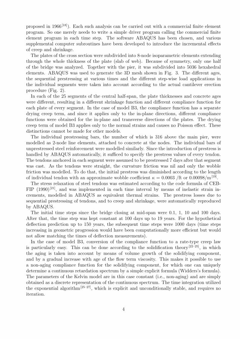
The plates of the cross section were subdivided into 8-node isoparametric elements extendingthrough the whole thickness of the plate (slab of web). Because of symmetry, only one halfof the bridge was analyzed. Together with the pier, it was subdivided into 5036 hexahedralelements. ABAQUS was used to generate the 3D mesh shown in Fig. 3. The different ages,the sequential prestressing at various times and the different step-wise load applications inthe individual segments were taken into account according to the actual cantilever erectionprocedure (Fig. 2).

In each of the 25 segments of the central half-span, the plate thicknesses and concrete ageswere different, resulting in a different shrinkage function and different compliance function foreach plate of every segment. In the case of model B3, the compliance function has a separatedrying creep term, and since it applies only to the in-plane directions, different compliancefunctions were obtained for the in-plane and transverse directions of the plates. The dryingcreep term of model B3 applies only to the normal strains and causes no Poisson effect. Thesedistinctions cannot be made for other models.

The individual prestressing bars, the number of which is 316 above the main pier, weremodelled as 2-node line elements, attached to concrete at the nodes. The individual bars ofunprestressed steel reinforcement were modelled similarly. Since the introduction of prestress ishandled by ABAQUS automatically, it sufficed to specify the prestress values of every tendon.The tendons anchored in each segment were assumed to be prestressed 7 days after that segmentwas cast. As the tendons were straight, the curvature friction was nil and only the wobblefriction was modelled. To do that, the initial prestress was diminished according to the lengthof individual tendon with an approximate wobble coefficient κ = 0.0003 /ft or 0.00098/m [19].

The stress relaxation of steel tendons was estimated according to the code formula of CEB-FIP (1990) [21], and was implemented in each time interval by means of inelastic strain in-crements, modelled in ABAQUS as equivalent thermal strains. The prestress losses due tosequential prestressing of tendons, and to creep and shrinkage, were automatically reproducedby ABAQUS.

The initial time steps since the bridge closing at mid-span were 0.1, 1, 10 and 100 days.After that, the time step was kept constant at 100 days up to 19 years. For the hypotheticaldeflection prediction up to 150 years, the subsequent time steps were 1000 days (time stepsincreasing in geometric progression would have been computationally more efficient but wouldnot allow matching the times of deflection measurements).

In the case of model B3, conversion of the compliance function to a rate-type creep lawis particularly easy. This can be done according to the solidification theory [22–25], in whichthe aging is taken into account by means of volume growth of the solidifying component,and by a gradual increase with age of the flow term viscosity. This makes it possible to usea non-aging compliance function for the solidifying component, for which one can uniquelydetermine a continuous retardation spectrum by a simple explicit formula (Widders’s formula).The parameters of the Kelvin model are in this case constant (i.e., non-aging) and are simplyobtained as a discrete representation of the continuous spectrum. The time integration utilizedthe exponential algorithm [25–27], which is explicit and unconditionally stable, and requires noiteration.

4

Despite prestress, calculations showed the top slab to get into tension after the first year.Large tensile cracks were not observed (JIAC [14], and ABAM [3] reports only sparsely locatedcracks in the first 6 segments from the mid-span). However, calculations that ignore the ten-sile strength limit f ′t revealed, for later years, tensile stresses several times larger than the f ′t .Because of this fact, due mainly to excessive prestress loss, a nonlinear tensile stress-strain rela-tion with a tensile strength limit was implemented in ABAQUS (thanks to dense reinforcement,capable of preventing localization of cracking, cohesive crack modeling was unnecessary). The

tensile strength was estimated as f ′t = 6psi√

f ′c/psi = 3.0 MPa (433 psi).It may be noted that core tests made before the retrofit revealed the porosity to be high and

the elastic modulus to be about 21.7 GPa, which was about 33% lower than that obtained byACI empirical formulas from the design compression strength and for the strength gain withage, which was 28.0 GPa. However, the low strength of cores was most likely a local deviationbecause matching of the mid-span deflection measured in the truck load test indicated theaverage elastic modulus of 23.5 GPa, which may be regarded as the average elastic modulusin the girder. Because of this fact, and because of uncertainty about the loading rate andtime delay in the truck test, the elastic modulus of concrete inferred from the compressionstrength according to the ACI formula was selected for comparing the design predictions basedon different models, including model B3, set 1 (defined later), while the calculations based onModel B3, set 2, used the elastic modulus calculated from the truck loading test which wasmade on this bridge.

As for tensile cracking, which must have taken place because of excessive prestress loss,its effect was not large, though not negligible either—the 19-year deflection with the tensilestrength limit was about 3% larger than it was for unlimited tensile strength.

The pavement layer of 76 mm (3 in.) thickness, which was made of a lower quality concretewith a unit weight about 5% smaller, was doubtless heavily cracked and was not anchoredagainst sliding over the top slab. Therefore, it was assumed incapable of resisting the appliedloads.

The microprestress-solidification theory [28], which allows a more accurate representation ofboth drying creep and aging, would have been more realistic. However, it would have requiredcalculating the distributions of pore relative humidity across the thickness of each slab, whichwould have necessitated not one but at least six finite elements over the slab thickness.

For the uniaxial compliance functions of models other than B3, the solidification theory can-not be applied. To incorporate them into the present step-by-step finite element computations,different discrete sets of spectral values of the retardation spectrum for different ages had to becalculated from the respective compliance functions and stored in advance of the finite elementstep-by-step analysis; see Appendix I. It was also verified that this calculation yields for modelB3 the same deflection curve as the solidification theory.

Creep and Shrinkage Models Considered

The deflections were analyzed on the basis of model B3 [22–25,29,30], the ACI model [31], the CEB(or CEB-FIP, fib) model [32], and the GL model of Gardner and Lockman [33,34]. The same 3Dfinite element analysis using ABAQUS, with Kelvin-chain based step-by-step integration intime (Appendix I), has been used for all these models.

The main material model used for the creep and shrinkage analysis was model B3, which wasfirst presented in Ref. [29], was slightly updated in Ref. [30], and was summarized in Ref. [25].It represented a refinement of the earlier BP and BP-KX models [35,36]. Theoretical justification

5

was provided in Ref. [28, 37, 38]. The B3 compliance function for basic creep was derived andexperimentally supported in Ref. [22-24]. In statistically unbiased comparisons with the mostcomplete database [39], model B3 came out as superior to other existing models [40,41].

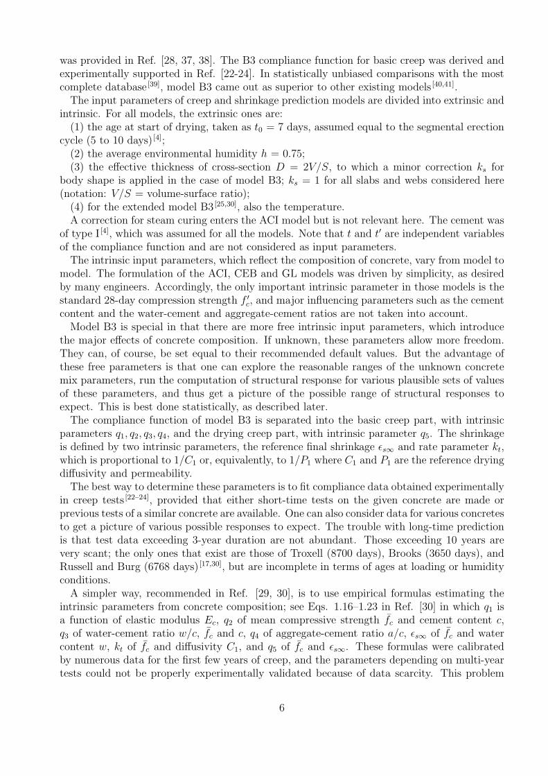
The input parameters of creep and shrinkage prediction models are divided into extrinsic andintrinsic. For all models, the extrinsic ones are:

(1) the age at start of drying, taken as t0 = 7 days, assumed equal to the segmental erectioncycle (5 to 10 days) [4];

(2) the average environmental humidity h = 0.75;(3) the effective thickness of cross-section D = 2V/S, to which a minor correction ks for

body shape is applied in the case of model B3; ks = 1 for all slabs and webs considered here(notation: V/S = volume-surface ratio);

(4) for the extended model B3 [25,30], also the temperature.A correction for steam curing enters the ACI model but is not relevant here. The cement was

of type I [4], which was assumed for all the models. Note that t and t′ are independent variablesof the compliance function and are not considered as input parameters.

The intrinsic input parameters, which reflect the composition of concrete, vary from model tomodel. The formulation of the ACI, CEB and GL models was driven by simplicity, as desiredby many engineers. Accordingly, the only important intrinsic parameter in those models is thestandard 28-day compression strength f ′c, and major influencing parameters such as the cementcontent and the water-cement and aggregate-cement ratios are not taken into account.

Model B3 is special in that there are more free intrinsic input parameters, which introducethe major effects of concrete composition. If unknown, these parameters allow more freedom.They can, of course, be set equal to their recommended default values. But the advantage ofthese free parameters is that one can explore the reasonable ranges of the unknown concretemix parameters, run the computation of structural response for various plausible sets of valuesof these parameters, and thus get a picture of the possible range of structural responses toexpect. This is best done statistically, as described later.

The compliance function of model B3 is separated into the basic creep part, with intrinsicparameters q1, q2, q3, q4, and the drying creep part, with intrinsic parameter q5. The shrinkageis defined by two intrinsic parameters, the reference final shrinkage εs∞ and rate parameter kt,which is proportional to 1/C1 or, equivalently, to 1/P1 where C1 and P1 are the reference dryingdiffusivity and permeability.

The best way to determine these parameters is to fit compliance data obtained experimentallyin creep tests [22–24], provided that either short-time tests on the given concrete are made orprevious tests of a similar concrete are available. One can also consider data for various concretesto get a picture of various possible responses to expect. The trouble with long-time predictionis that test data exceeding 3-year duration are not abundant. Those exceeding 10 years arevery scant; the only ones that exist are those of Troxell (8700 days), Brooks (3650 days), andRussell and Burg (6768 days) [17,30], but are incomplete in terms of ages at loading or humidityconditions.

A simpler way, recommended in Ref. [29, 30], is to use empirical formulas estimating theintrinsic parameters from concrete composition; see Eqs. 1.16–1.23 in Ref. [30] in which q1 isa function of elastic modulus Ec, q2 of mean compressive strength fc and cement content c,q3 of water-cement ratio w/c, fc and c, q4 of aggregate-cement ratio a/c, εs∞ of fc and watercontent w, kt of fc and diffusivity C1, and q5 of fc and εs∞. These formulas were calibratedby numerous data for the first few years of creep, and the parameters depending on multi-yeartests could not be properly experimentally validated because of data scarcity. This problem

6

particularly afflicts the formulas for q3 (the non-aging viscoelastic term) and q4 (the flow term),because they govern mainly the long-time creep.

Two sets of input parameters have been considered in computations:Set 1: For the simple prediction on the basis of concrete composition, the following input

has been used:(1) the mean compressive strength at 28 days, which is the only relatively certain input

parameter for the KB Bridge; it was estimated as f ′cr = 35.9 MPa (5200 psi) from the speci-fied design strength f ′c = 34.5 MPa (5000 psi) [6], under the assumption of a typical standarddeviation;

(2) the 28-day elastic modulus, not known but estimated as Ec = (57, 000 psi)√

f ′cr/psi, which

gives Ec = 28.3 GPa (4110 ksi).(3) c = 620 lb/yd3, a/c = 3 and w/c = 0.62 [4].The result was:

q1 = 0.149, q2 = 1.02, q3 = 0.044, q4 = 0.065, q5 = 2.27 (10−6/psi) (1)

εk∞ = 0.0011 and kt = 16 (Set 1) (2)

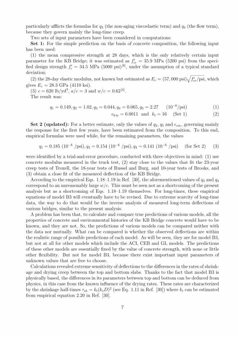
Set 2 (updated): For a better estimate, only the values of q2, q5 and εs∞, governing mainlythe response for the first few years, have been estimated from the composition. To this end,empirical formulas were used while, for the remaining parameters, the values

q1 = 0.185 (10−6 /psi), q3 = 0.154 (10−6 /psi), q4 = 0.141 (10−6 /psi) (for Set 2) (3)

were identified by a trial-and-error procedure, conducted with three objectives in mind: (1) useconcrete modulus measured in the truck test, (2) stay close to the values that fit the 23-yearcreep tests of Troxell, the 18-year tests of Russel and Burg, and 10-year tests of Brooks, and(3) obtain a close fit of the measured deflection of the KB Bridge.

According to the empirical Eqs. 1.18–1.19 in Ref. [30], the aforementioned values of q3 and q4

correspond to an unreasonably large w/c. This must be seen not as a shortcoming of the presentanalysis but as a shortcoming of Eqs. 1.18–1.19 themselves. For long-times, these empiricalequations of model B3 will eventually have to be revised. Due to extreme scarcity of long-timedata, the way to do that would be the inverse analysis of measured long-term deflections ofvarious bridges, similar to the present analysis.

A problem has been that, to calculate and compare true predictions of various models, all theproperties of concrete and environmental histories of the KB Bridge concrete would have to beknown, and they are not. So, the predictions of various models can be compared neither withthe data nor mutually. What can be compared is whether the observed deflections are withinthe realistic range of possible predictions of each model. As will be seen, they are for model B3,but not at all for other models which include the ACI, CEB and GL models. The predictionsof these other models are essentially fixed by the value of concrete strength, with none or littleother flexibility. But not for model B3, because there exist important input parameters ofunknown values that are free to choose.

Calculations revealed extreme sensitivity of deflections to the differences in the rates of shrink-age and drying creep between the top and bottom slabs. Thanks to the fact that model B3 isphysically based, the differences in its parameters between top and bottom can be deduced fromphysics, in this case from the known influence of the drying rates. These rates are characterizedby the shrinkage half-times τsh = kt(ksD)2 (see Eq. 1.11 in Ref. [30]) where kt can be estimatedfrom empirical equation 2.20 in Ref. [30].

7

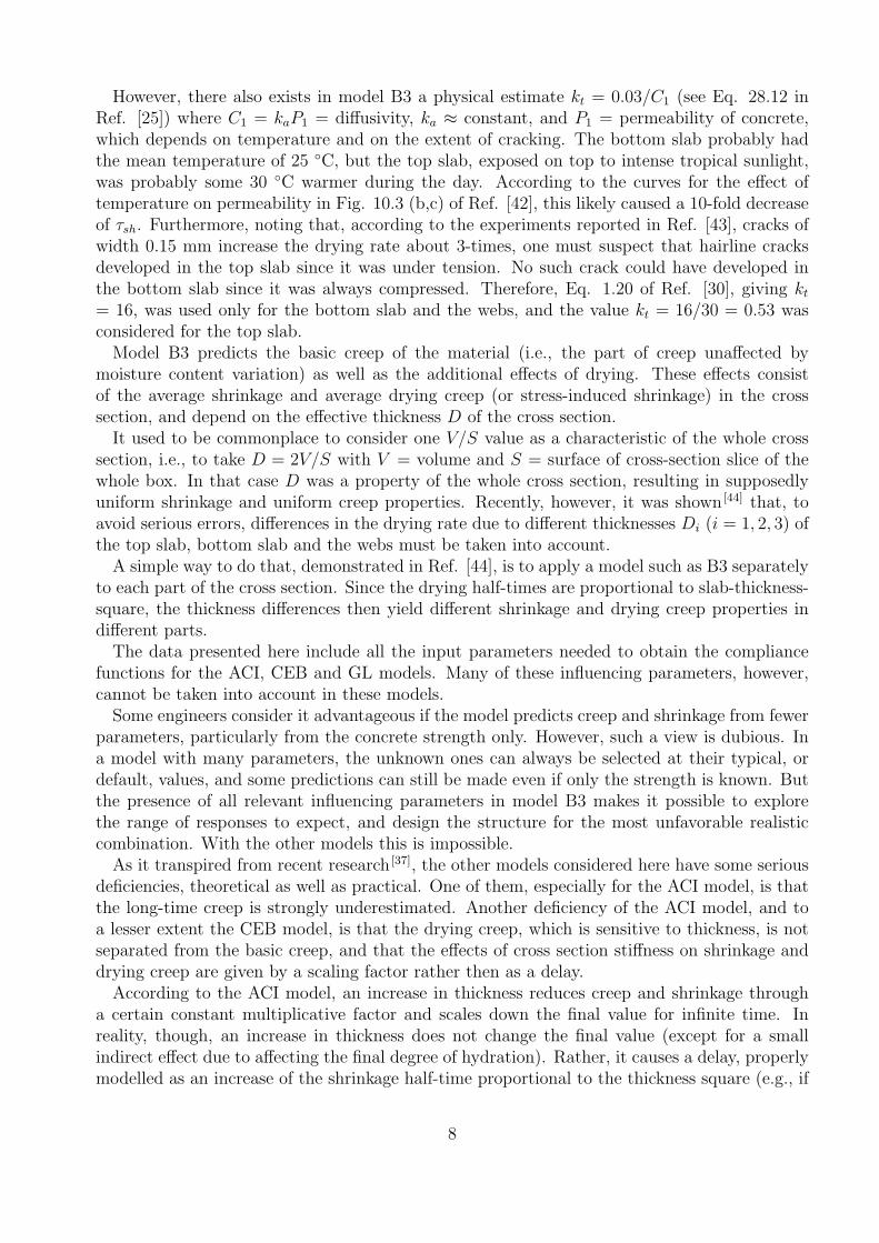
However, there also exists in model B3 a physical estimate kt = 0.03/C1 (see Eq. 28.12 inRef. [25]) where C1 = kaP1 = diffusivity, ka ≈ constant, and P1 = permeability of concrete,which depends on temperature and on the extent of cracking. The bottom slab probably hadthe mean temperature of 25 ◦C, but the top slab, exposed on top to intense tropical sunlight,was probably some 30 ◦C warmer during the day. According to the curves for the effect oftemperature on permeability in Fig. 10.3 (b,c) of Ref. [42], this likely caused a 10-fold decreaseof τsh. Furthermore, noting that, according to the experiments reported in Ref. [43], cracks ofwidth 0.15 mm increase the drying rate about 3-times, one must suspect that hairline cracksdeveloped in the top slab since it was under tension. No such crack could have developed inthe bottom slab since it was always compressed. Therefore, Eq. 1.20 of Ref. [30], giving kt

= 16, was used only for the bottom slab and the webs, and the value kt = 16/30 = 0.53 wasconsidered for the top slab.

Model B3 predicts the basic creep of the material (i.e., the part of creep unaffected bymoisture content variation) as well as the additional effects of drying. These effects consistof the average shrinkage and average drying creep (or stress-induced shrinkage) in the crosssection, and depend on the effective thickness D of the cross section.

It used to be commonplace to consider one V/S value as a characteristic of the whole crosssection, i.e., to take D = 2V/S with V = volume and S = surface of cross-section slice of thewhole box. In that case D was a property of the whole cross section, resulting in supposedlyuniform shrinkage and uniform creep properties. Recently, however, it was shown [44] that, toavoid serious errors, differences in the drying rate due to different thicknesses Di (i = 1, 2, 3) ofthe top slab, bottom slab and the webs must be taken into account.

A simple way to do that, demonstrated in Ref. [44], is to apply a model such as B3 separatelyto each part of the cross section. Since the drying half-times are proportional to slab-thickness-square, the thickness differences then yield different shrinkage and drying creep properties indifferent parts.

The data presented here include all the input parameters needed to obtain the compliancefunctions for the ACI, CEB and GL models. Many of these influencing parameters, however,cannot be taken into account in these models.

Some engineers consider it advantageous if the model predicts creep and shrinkage from fewerparameters, particularly from the concrete strength only. However, such a view is dubious. Ina model with many parameters, the unknown ones can always be selected at their typical, ordefault, values, and some predictions can still be made even if only the strength is known. Butthe presence of all relevant influencing parameters in model B3 makes it possible to explorethe range of responses to expect, and design the structure for the most unfavorable realisticcombination. With the other models this is impossible.

As it transpired from recent research [37], the other models considered here have some seriousdeficiencies, theoretical as well as practical. One of them, especially for the ACI model, is thatthe long-time creep is strongly underestimated. Another deficiency of the ACI model, and toa lesser extent the CEB model, is that the drying creep, which is sensitive to thickness, is notseparated from the basic creep, and that the effects of cross section stiffness on shrinkage anddrying creep are given by a scaling factor rather then as a delay.

According to the ACI model, an increase in thickness reduces creep and shrinkage througha certain constant multiplicative factor and scales down the final value for infinite time. Inreality, though, an increase in thickness does not change the final value (except for a smallindirect effect due to affecting the final degree of hydration). Rather, it causes a delay, properlymodelled as an increase of the shrinkage half-time proportional to the thickness square (e.g., if

8

the ultimate shrinkage of a slab 0.10 m thick is reached in 10 years, for a slab 1 m thick it isreached in 1000 years, i.e., virtually never).

Calculated Deflections and Prestress Loss, and Comparisons to Mea-surements

As a first check of the finite element code, comparison was made with the bridge stiffness,which was measured in January 1990 by Japan International Cooperation Agency (JICA). Adownward deflection of 0.10 ft. (30.5 mm) was recorded at mid-span when two 12.5 ton truckswere parked on each side of the mid-span hinge (one previous paper erroneously assumed thatonly one truck was on each side). The finite element code based on model B3 predicted thedeflection of 0.098 ft. (30 mm) under the load of 250 kN that was applied gradually within 2.4hours. Given the uncertainty about the actual rate of loading, the difference is small enough.

The results of calculations are shown in figures 4–8, both in linear and logarithmic time scales(t = time measured from the start of construction, and t1 = duration of the construction). Thedata points show the measured values. The solid diamonds represent the data reported bythe firm investigating the collapse [7], and the solid circles the data accepted from a secondarysource [14]. For comparison, the figures show the results obtained with model B3 and the ACI,CEB and GL models. All these responses have been computed with the same finite elementprogram and the same step-by-step time integration algorithm, in which the different thicknessesof the slabs and webs were considered. The response of the GL model is also shown for thetotal deflection curve (Fig. 4 and Fig. 5).

Fig. 4 shows the deflection curves up to the moment of retrofit at about 19 years of age.Since well designed bridges (such as the Brooklyn Bridge) have lasted much longer, Fig. 5shows the same curves extended up to 150 years under the assumption that there has been noretrofit and no collapse.

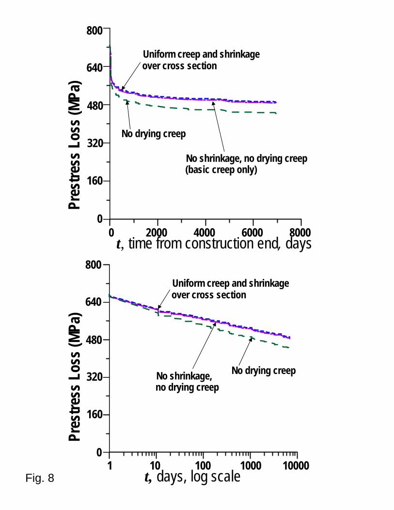
Figures 7–8 clarify the mid-span deflection and prestress loss obtained (1) if the drying creepis neglected, (2) if both the shrinkage and drying creep are neglected, and (3) if the creep andshrinkage properties are considered to be uniform over the cross section, based on the effectivethickness D = 2V/S for the whole cross section. Note that the use of uniform creep andshrinkage properties throughout the cross section neglects the effects of differential shrinkageand differential drying creep and gives results very close to those for basic creep alone.

Accuracy in calculating the prestress loss is essential because the bridge deflection is a smalldifference of two large but uncertain numbers—the downward deflection due to self-weight, andthe upward deflection due to prestress. For the sake of illustration, compared to the classicaltheory of bending, the shear lag increased the elastic downward deflection due to self-weight by18%, and the elastic upward deflection due to initial prestress by 14%, and the total deflectionby 30%.

The measured 18-year deflection, which was 1.39 m, is matched by the deflection calculatedfrom model B3 (set 2). This measured deflection is about 3-times larger than those calculatedfor the ACI, CEB (which are 0.47 m and 0.53 m), and about the double of that from the GLmodel (which is 0.65 m); see Fig. 4. Besides, the ACI, CEB and GL deflection curves haveshapes rather different from model B3. They give too much deflection during the first year,and far too little from 3 years on, especially for the ACI and CEB models. An important pointto note is that the 18-year prestress loss is less than 30% when the ACI and CEB models areused in the present three-dimensional finite element calculations, but about 46% when modelB3 is used (Fig. 6).

9

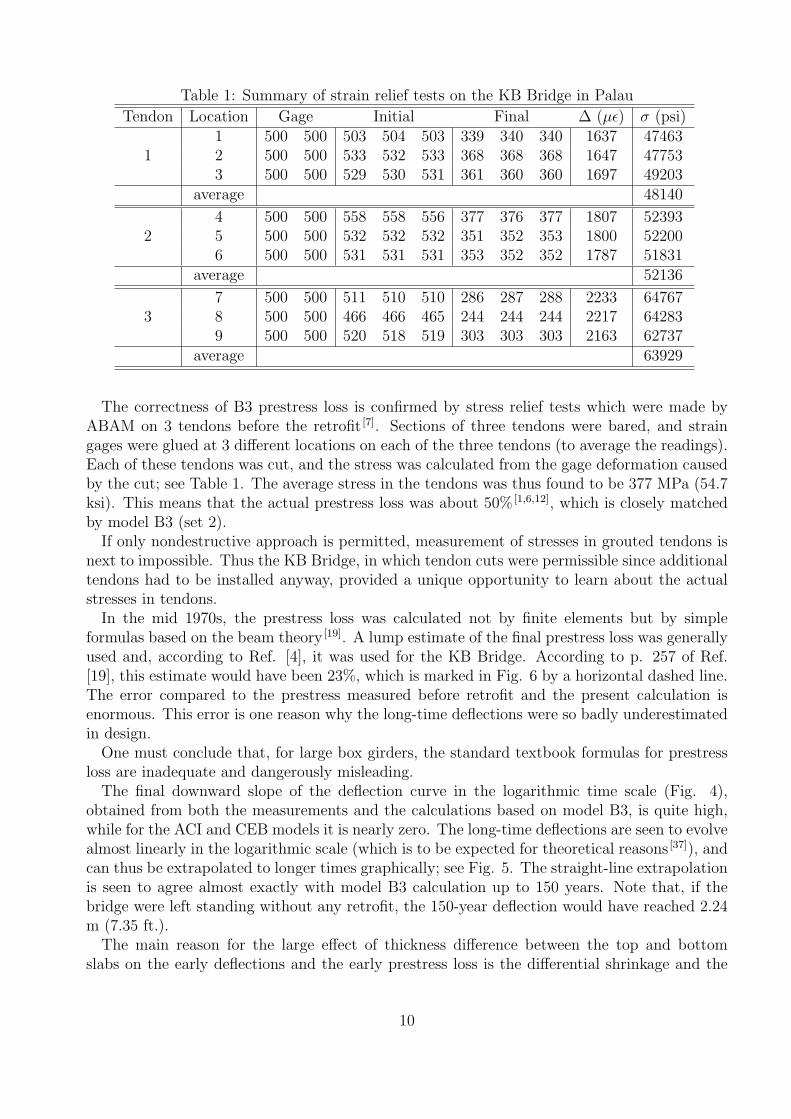
Table 1: Summary of strain relief tests on the KB Bridge in Palau

Tendon Location Gage Initial Final ∆ (µε) σ (psi)1 500 500 503 504 503 339 340 340 1637 47463

1 2 500 500 533 532 533 368 368 368 1647 477533 500 500 529 530 531 361 360 360 1697 49203

average 48140

4 500 500 558 558 556 377 376 377 1807 523932 5 500 500 532 532 532 351 352 353 1800 52200

6 500 500 531 531 531 353 352 352 1787 51831average 52136

7 500 500 511 510 510 286 287 288 2233 647673 8 500 500 466 466 465 244 244 244 2217 64283

9 500 500 520 518 519 303 303 303 2163 62737average 63929

The correctness of B3 prestress loss is confirmed by stress relief tests which were made byABAM on 3 tendons before the retrofit [7]. Sections of three tendons were bared, and straingages were glued at 3 different locations on each of the three tendons (to average the readings).Each of these tendons was cut, and the stress was calculated from the gage deformation causedby the cut; see Table 1. The average stress in the tendons was thus found to be 377 MPa (54.7ksi). This means that the actual prestress loss was about 50% [1,6,12], which is closely matchedby model B3 (set 2).

If only nondestructive approach is permitted, measurement of stresses in grouted tendons isnext to impossible. Thus the KB Bridge, in which tendon cuts were permissible since additionaltendons had to be installed anyway, provided a unique opportunity to learn about the actualstresses in tendons.

In the mid 1970s, the prestress loss was calculated not by finite elements but by simpleformulas based on the beam theory [19]. A lump estimate of the final prestress loss was generallyused and, according to Ref. [4], it was used for the KB Bridge. According to p. 257 of Ref.[19], this estimate would have been 23%, which is marked in Fig. 6 by a horizontal dashed line.The error compared to the prestress measured before retrofit and the present calculation isenormous. This error is one reason why the long-time deflections were so badly underestimatedin design.

One must conclude that, for large box girders, the standard textbook formulas for prestressloss are inadequate and dangerously misleading.

The final downward slope of the deflection curve in the logarithmic time scale (Fig. 4),obtained from both the measurements and the calculations based on model B3, is quite high,while for the ACI and CEB models it is nearly zero. The long-time deflections are seen to evolvealmost linearly in the logarithmic scale (which is to be expected for theoretical reasons [37]), andcan thus be extrapolated to longer times graphically; see Fig. 5. The straight-line extrapolationis seen to agree almost exactly with model B3 calculation up to 150 years. Note that, if thebridge were left standing without any retrofit, the 150-year deflection would have reached 2.24m (7.35 ft.).

The main reason for the large effect of thickness difference between the top and bottomslabs on the early deflections and the early prestress loss is the differential shrinkage and the

10

difference in the drying creep compliance between the top and bottom slabs. In a previousstudy of the effect of thickness difference between the top and bottom slabs on deflections [44],the effect of differential drying creep was found to be small in comparison to the effect ofdifferential shrinkage. Here the difference in drying creep compliance is almost as importantas the differential shrinkage. The reason is that initially the prestress in the top slab is highenough to cause a high drying creep.

A typical feature of prestressed box girders erected as segmental cantilevers is that initially,during the first 1 month to 3 years, the deflections are negative, i.e., upwards [44]. Measurementsto confirm this behavior for the KB Bridge are unavailable. However, the present calculationssupport it (Fig. 4).

Altogether, one can identify four principal reasons why the measured deflections can bematched by model B3 (set 2) but not the ACI, CEB and GL models:

(1) A significantly higher long-time creep in model B3, compared to the ACI, CEB andGL models. There are three reasons for that: a) theoretical advances during the last threedecades, incorporated in model B3 [25,30,37]; b) model calibration by a larger database, with arational statistical calibration procedure compensating for the database bias for short timesand for small specimen sizes [39,45]; and c) adjustment of the model to the shape of creep curvesobserved in individual long-time tests (5 to 25 years), which is obscured when the database isonly considered as a whole [31].

(2) Three-dimensional analysis of deflections and prestress loss, which is more realistic thanthe beam bending analysis, especially because it can capture different effects of shear lag onthe downward deflection due to self-weight and the upward deflection due to prestress.

(3) Realistic representation of nonuniform shrinkage and drying creep properties in the crosssections, caused by the effect of different wall and slab thicknesses on the shrinkage and dryingcreep rates and half-times, as well as by the differences in permeability due to temperaturedifferences and cracking.

(4) A larger number of input parameters in model B3, which include the water-cement ratioand aggregate-cement ratio. This allows a greater range of responses to be explored in design,compared to the ACI, CEB and CL models. These models are inflexible because of missingthese input parameters, and thus provide a unique response if the strength of concrete is fixed.

Uncertainty of Deflection Predictions and Calculation of ConfidenceLimits

Creep and shrinkage are notorious for their relatively high random scatter. For this reason,it has been argued for the last two decades that the design should be made not for the meandeflections, but for some suitable confidence limits such as 95% [40,46]. Adopting the Latinhypercube sampling of input parameters [46], one can easily obtain such confidence limits byrepeating the deterministic computer analysis of the bridge 8-times, one run for each of 8different randomly generated samples of 8 input parameters.

The range of the cumulative distribution of each random input variable (assumed to be Gaus-sian) is partitioned into N intervals of equal probability. The parameter values corresponding tothe centroids of these intervals are selected according to randomly generated Latin hypercube ta-bles (which can be freely downloaded from the ITI website–http://iti.northwestern.edu/generator,so that a bridge designer would not need to work with a random number generator at all). Thevalues from the rows of these tables are then used as the input parameter for N deterministiccomputer runs of creep and shrinkage analysis.

11

By experience, it is sufficient to chose N = n = number of random input parameters (hereN = n = 8). One random input variable is the environmental relative humidity h, whose meanand coefficient of variation are estimated as 0.75 and 0.2 (or 75% and 20%). The others arethe material characteristics q1, q2, q3, q4, q5, kt and ε∞, representing the parameters of model B3.According to model B3, the means of these parameters for the KB Bridge are found to be:q1 = 0.185, q2 = 0.102, q3 = 0.132, q4 = 0.141, q5 = 2.27, kt = 16.05, and ε∞ = 0.0011. Theestimated coefficient of variation is 23% for creep parameters q1, q2, q5 and 30% for q3, q4 (whichis higher because of uncertainty and scarcity of long-term creep data), and 34% for shrinkageparameters kt = 16 and ε∞.

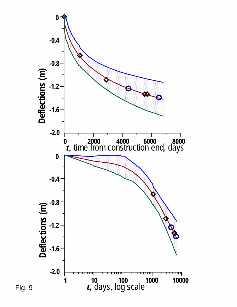
The responses from each deterministic computer run for model B3 (set 2), particularly themid-span deflections at specified times, are collected in one histogram of 8 values, whose meanw and coefficient of variation ωw are the desired statistics. Knowing these, and assuming theGaussian (or normal) distribution, one can get the one-sided 95% confidence limit as w95 =w(1 + 1.645ωw) (which is exceeded with the probability of 5%; in other words, one out of 20identical bridges would exceed that limit, which seems to give optimal balance between riskand cost).

The curves of the mean, and of the one-sided 95% and 5% confidence limit for the KB Bridgein Palau, are shown (for model B3, set 2) in Fig. 9. Note that the curves of the presentfinite element calculations according to the ACI and CEB models lie way outside the statisticalconfidence band obtained with model B3 (and the traditional prediction lies even farther).

The probabilistic problem of deflections is fortunately much simpler than that of structuralsafety. For the latter, the extreme value statistical theory must be used since the tolerableprobability of failure is < 10−6, far less than the value of 0.05 acceptable for deflections.

Comparison with Analysis by Bending Theory with Plane Cross Sec-tions

Traditionally, box girders have been analyzed according to the classical engineering theory ofbending in which the cross sections are assumed to remain plane. However this engineeringtheory of bending is too simplified to capture the deformation of box girders accurately. Itsmain deficiency is that it lacks the effect of shear lag, both in the top slab and in the web, andboth for self weight and for prestress. In Fig. 10, the distribution of shear stress in a crosssection located at 7.08 m (23.3 ft.) away from main pier face, is shown when only self weightor only prestress is considered. It can be seen that a significant shear stress exists in the topand bottom slabs.

The total deflection is sensitive because it represents a small difference of two large numberscorresponding to self weight and to prestress. The shear lag plays a more important role indownward deflection by self weight than upward deflection by prestress. Therefore the neglectof shear lag may lead to a considerable underestimation of the long-term deflection.

The significant discrepancy between full 3D simulation and engineering theory of bending isdemonstrated in Fig. 11. The deflections and prestress losses obtained in this classical way forB3, ACI, CEB and GL models are compared with 3D analysis. A large error, which is about30% less in long-term deflection, is found for this classical engineering approach.

In the KB Bridge design, an approximate correction for the shear lag in the top slab dueto self weight was introduced [4] through the classical effective width concept [47–51]. For totaldeflections, however, this classical concept can still give major errors compared to the full 3Danalysis.

12

Causes of Excessive Deflections and Lessons Learned

As confirmed by this study, the following ten points are essential for correctly predicting thelong-time response of bridges highly sensitive to creep and shrinkage.

1. The 1972 ACI model (reapproved in 2007 [31]), and to a lesser extent the CEB model, areobsolete. They severely underestimate the long-time deflections as well as the prestresslosses, for a number of reasons [37]. They lack a solid theoretical foundation, do not reflectthe theoretical advances of the last three decades [37], and have not been experimentallycalibrated by a large and complete database [30] using a sound statistical method [39,45] off-setting statistical bias. The recent GL model gives better predictions, but not sufficientlybetter (its long-term creep is too low, the model does not have enough intrinsic inputparameters, the effect of temperature and cracking on diffusivity cannot be accountedfor, etc.)

2. The effect of thickness differences among the webs and top and bottom slabs on shrinkageand drying creep must be taken into account. This leads to non-uniform creep andshrinkage properties throughout the cross section, manifested as differential drying creepand differential shrinkage.

3. Because of its thickness dependence, the drying creep should be separated in the predictionmodel from the basic creep, which is independent of thickness. As evidenced by the KBBridge, the thickness-induced differences in the compliance functions for drying creep canbe as important as those in shrinkage.

4. The effect of slab or web thicknesses on the drying creep rate and the shrinkage ratemust be taken into account. This means that the half-time of shrinkage and drying creepshould be proportional to the thickness square and their curves should initially evolve asa square root of time (as dictated by the diffusion theory [37]). Further it is appropriateto take into account the effect of temperature differences on the drying rates.

5. The prestress loss may be 2- to 3-times higher than predicted by simple textbook formulasor lump estimates. It can also be much higher than that predicted by the theory of beambending in which the cross sections remain plane. The loss should be calculated as partof 3D finite element analysis, using a sound creep and shrinkage model and taking intoaccount the nonuniformity of shrinkage and drying creep properties throughout the crosssection.

6. The main reason why a 3D analysis is necessary is that it automatically captures the effectof shear lag, as well as the effects of differential shrinkage and drying creep. The neglectof shear lag, which causes a nonlinear distribution of normal stresses over the slabs andthe webs within the cross section, leads to underestimation of deflections and prestresslosses.

7. The shear lag effects on deflections due to self weight and to prestress are different. Theself weight produces large vertical shear forces in the web at the piers, but the prestressdoes not. Thus the shear lag is strong for the self weight but weaker for the prestress.Since the total deflection is a small difference of two large numbers, one for the downwarddeflection due to self-weight and the other for the upward deflection due to prestress,a small percentage error in the first, typically 10% to 15%, will result in a far largerpercentage error in the total deflection.

13

8. When dealing with large creep-sensitive structures, updating of the creep and shrinkageprediction based on short-time tests of the given concrete is necessary. However, evenwhen short-time tests were made for some structures in the past, their conduct has usuallybeen incorrect. Previous research showed that an order-of-magnitude error reduction inthe long-time creep and shrinkage predictions can be achieved with model B3 by meansof updating on the basis of one-month creep and shrinkage tests of the particular concreteto be used, provided that they are accompanied by water loss measurements [30]. Suchtests were not made for the KB Bridge, but have met with success for some recent largebridges [52]. B3 is a model that has been specifically formulated so as to allow easy updatingby linear regression, while for other models the updating problem is nonlinear.

9. Large bridges should be designed not for the mean but for 95% confidence limit on thepredicted deflection (in other words, having to repair or close more than 1 bridge in20 is unacceptable). The necessary statistical analysis is easy. It suffices to repeat adeterministic computer run of structural response about ten-times, using properly selectedrandom samples of the input parameters. Then one needs to evaluate the mean andvariance of the calculated response values. Assuming a normal distribution, one has itsboth parameters, and from a table of normal distribution the confidence limit then follows.

10. As observed in Ref. [44], the deflection evolution of large box girders is usually counterin-tuitive. The deflections grow slowly or are even negative during the first months or years,which often leads to unwarranted optimism. Later, unfortunately, a rapid and excessivedeflection growth sets in. The early deflections of the KB bridge were not measured, butaccording to the present calculations the bridge must have been deflecting upward for aninitial period of up to 2 months (Fig. 4).

Closing Comments

If the models and methods available today were used at the time of design, the observeddeflections of the KB Bridge in Palau would have been expected. This would have forced aradical change of design of this bridge.

The results obtained for the ACI model [5,31,54] (Figs. 4–6) document that this model canlead to dangerous underprediction of deflections and prestress losses. Yet this ACI model,first introduced in 1972, has recently been reapproved by ACI and is featured as one of therecommended models in ACI Guide 209.2R-08 [31] (the appearance of the first writer’s name onthe list of the authoring committee was mandatory and did not imply his endorsement of thisGuide). Similar though milder objections apply to the CEB and GL models.

The experience with the KB Bridge and the present analysis confirms computationally theprevious experience that bridges with a sliding hinge at mid-span are too vulnerable and shouldbe avoided. Continuous box girders give significantly smaller deflections. It is worth notingthat the Brooklyn bridge (span 486 m, built in 1883) and the Firth-of-Forth Bridge (span 510m, built in 1890), which both held world records, are still in service today. In view of Fig. 5,nothing close to such a lifespan can be expected for the large prestressed concrete box girderswhich were designed using simple material models and simplified methods of analysis.

Designs that mitigate deflections should be sought. Continuous box girders deflect signifi-cantly less than those with a hinge at mid-span, as is already well known. In continuous girders,the deflections are particularly sensitive to tendon layout [53] and can be reduced by the right

14

layout. A layout benefiting the stress state can at the same time be harmful from the deflectionviewpoint.

Insufficient efforts have, unfortunately, been made in the past to transfer the results of ex-perimental and theoretical research on creep and shrinkage into practice. At the same time,these results have unjustly been regarded by many practitioners as irrelevant and artificiallycomplex academic exercises. Many of the causes of excessive deflections of the KB bridge werein principle known from research papers already in the early 1970s [47–51,55–67]; they included theshear lag effect, the true effect of slab thickness on the drying-induced strains, the use of timecurves that underpredict the long-term creep and ignore the long-time experimental data [60],and accurate step-by-step time integration of structural concrete creep problems by the expo-nential algorithm. The analysis of these causes was not impossible in the early 1970s, however,nobody at that time realized their importance, and even if someone did, a supercomputer ofthose times would have been required.

Acknowledgment. Financial support from the U.S. Department of Transportation throughGrant 0740-357-A222 from the Infrastructure Technology Institute of Northwestern University,is gratefully appreciated. Thanks are due to Dr. Khaled Shawwaf of DSI, Inc., Bolingbrook,Illinois, for providing valuable information on the analysis, design and investigations of thisrecord-setting bridge.

Appendix I. Simpler Variant of Step-by-Step Creep Structural Anal-ysis for Empirical Compliance Function

Accurate and efficient creep analysis requires replacing the constitutive law with a history in-tegral based on the principle of superposition by a rate-type creep law with internal variablesbased on the viscoelastic Kelvin chain model [15–17,25]. The rate-type creep formulation is par-ticularly simple for the solidification theory underlying model B3 because the creep propertiescan be specified by the non-aging properties of the hardening constituent whose volume growthaccounts for aging, which means that the spectrum of elastic moduli of the Kelvin chain unitsis constant in time and can be identified by an explicit formula from the compliance curve.

A method that simplifies programming at the expense of letting more data and more com-putations to be handled by the computer has now been devised. In numerical step-by-stepstructural analysis, the retardation spectrum is needed only for the discrete ages of concretecorresponding to the middle of the chosen time steps (for the KB bridge, 10 time steps increas-ing in geometric progression were used to obtain the solution up to 19 years, and 15 steps upto 150 years).

For empirical models such as those of ACI, CEB and GL, the creep analysis is more com-plicated since a non-aging constituent corresponding to the solidification theory cannot beidentified for these models. Therefore, compliance curves that change with the age at loadingmust be used.

Such a situation was handled in the 1970s by considering the retardation (or relaxation)spectrum, to be age dependent, which meant that the spectrum of elastic moduli of the Kelvin(or Maxwell) chain model to be considered as age-dependent [15–17]. Identification of thesemoduli as functions of age was not unambiguous.

For the loading age corresponding to each time step, the ACI, CEB or GL model gives onecompliance curve (or unit creep curve), for which the continuous retardation spectrum can beobtained by Widder’ explicit formula for inversion of Laplace transform [68]. This continuous

15

retardation spectrum is then approximated by a set of discrete spectral values Di, one setfor each time step. These spectral values are then used in the individual time steps of theexponential algorithm based on Kelvin chain (as described in Ref. [15-17]). No continuousfunction for Di(t), which complicated the previous practice, need be identified and used.

Appendix II: Resolution of 3rd Structural Engineers World Congresson Data Disclosure Ethics

In Bangalore, India, on November 6, 2007, this Congress adopted the following resolution:

1. The structural engineers gathered at their 3rd World Congress deplore the fact the technicaldata on the collapses of various large structures, including the Koror-Babeldaob Bridge inPalau, have been sealed as a result of legal litigation.

2. They believe that the release of all such data would likely lead to progress in structuralengineering and possibly prevent further collapses of large concrete structures.

3. In the name of engineering ethics, they call for the immediate release of all such data.

This resolution was proposed at the congress by Z.P. Bazant, in the name of the followinggroup of experts whose support has been solicited in advance: P. Marti (ETH), F.J. Ulm(MIT), A. Ingraffea (Cornell University), W. Dilger (U. of Calgary), P. Gambarova, L. Cedolin,G. Maier (Politecnico di Milano), E. Fairbairn (Rio de Janeiro), W. Gerstle (U. of New Mexico),K. Willam (UC Boulder), V. Kristek (CVUT Prague), T.P. Chang (Taipei) J.C. Chern (Taipei),T. Tanabe (Nagoya), C. Leung (HKUST, Hong Kong), M. Jirasek (CVUT Prague), D. Novak,M. Vorechovsky (VUT Brno), M. Kazemi (Tehran), Susanto Teng (Singapore), R. Eligehausen,J. Ozbolt (Stuttgart U.), B. Schrefler, C. Majorana (U. of Padua), Zongjin Li (HKUST, HongKong), K. Maekawa (U. of Tokyo), C. Videla (Santiago), J.G. Rots (Delft), S. Teng (Singapore),H. Mihashi (Sendai), H. Mang (Vienna), B. Raghu-Prasad (Bangalore), N. Bicanic (Glasgow),I. Robertson (Honolulu), J. van Mier (Zurich), Z.J. Li (Hong-Kong), K. Maekawa (Tokyo),V. Saouma (Boulder), Y. Xi (Boulder), L. Belarbi (Missouri), L. Elfgren (Lulea), C. Andrade(Madrid), I. Carol (Barcelona), D.M. Frangopol (Lehigh), J.W. Ju (Los Angeles), T. Tsubaki(Yokohama), N.M. Hawkins (Seattle), J.-K. Kim (Korea), A. Zingoni (Cape Town).

Appendix III: Similar Excessive Deflections Documented for JapaneseBridges

Dr. Yasumitsu Watanabe, the chief engineer of Shimizu Construction Corporation, Tokyo,documented at Concreep-8 (Ise-Shima, Japan, September 30, 2008) that many Japanese boxgirders also deflected far more than predicted by the traditional method based based on theJSCE design code. He graciously made available to the writers the deflection data on fourmonitored bridges shown in Figs. 12-15. Note the similarity to the bridge in Palau, andespecially the steep increase of long-time deflections seen in the logarithmic time scale.

16

References[1] Yee, A.A. (1979). “Record span box girder bridge connects Pacific Islands” Concrete International

1 (June), pp. 22–25.

[2] Comite euro-international du beton (CEB) (1978) Bulletin d’Information No. N. 124/125-E,Paris, France.

[3] ABAM Engineers Inc. (1993). Basis for design, Koror-Babeldaob bridge repairs.

[4] Private conversation with K., Shawwaf who was a member of the design team of KB bridge,September 18, 2008.

[5] ACI Committee 209 (1971) “Prediction of creep, shrinkage and temperature effects in concretestructures” ACI-SP27, Designing for Effects of Creep, Shrinkage and Temperature, Detroit, pp.51–93.

[6] McDonald, B., Saraf, V., and Ross, B. (2003). “A spectacular collapse: The Koro-Babeldaob(Palau) balanced cantilever prestressed, post-tensioned bridge” The Indian Constrete JournalVol. 77, No.3, March 2003, pp. 955–962.

[7] Berger/ABAM Engineers Inc. (1996). KB Bridge modifications and repairs.

[8] SSFM Engineers, Inc. (1996) Preliminary Assessment of Korror-Babeldaob Bridge Failure, pre-pared for US Army Corps of Engineers, October 2, 1996.

[9] Parker, D. (1996). “Tropical Overload”, New Civil Engineer, December 5, 1996.

[10] Pilz, M. (1997). The collapse of the KB bridge in 1996, Dissertation, Imperial College London.

[11] Pilz, M. (1999). “Untersuchungen zum Einsturzder KB Brucke in Palau”, Beton- und Stahlbeton-bau, May 1999, 94/5.

[12] Burgoyne, C. and Scantlebury, R. (2006). “Why did Palau bridge collapse?” The StructuralEngineer, pp. 30-37.

[13] ABAM Engineers Inc. (1993). Record of telephone conversation, Aug. 13, 1993.

[14] Japan International Cooperation Agency (1990). Present Condition Survey of the Koror-Babelthuap Bridge, Feburary, 1990.

[15] Bazant, Z.P. (1975).“Theory of creep and shrinkage in concrete structures: A precise of recentdevelopments” Mechanics Today, ed. by S. Nemat-Nasser (Am. Acad. Mech.), Pergamon Press1975, Vol. 2, pp. 1–93.

[16] Bazant, Z.P. (1982). “Mathematical models of nonlinear behavior and fracture of concrete” inNonlinear Numerical Analysis of Reinforced Concrete, ed. by L. E. Schwer, Am. Soc. of Mech.Engrs., New York, 1–25.

[17] RILEM Committee TC-69 (1988). “State of the art in mathematical modeling of creep andshrinkage of concret” in Mathematical Modeling of Creep and Shrinkage of Concrete, ed. by Z.P.Bazant, J. Wiley, Chichester and New York, 1988, 57–215.

[18] Bazant, Z.P. (1967) “Linear creep problems solved by a succession of generalized thermoelasticityproblems” Acta Technica CSAV, 12, pp. 581–594.

[19] Nilson, A.H. (1987). Design of Prestressed Concrete, 2nd edition, John Wiley & Sons, New York.

[20] PCI Committee (1975). “Recommendations for estimating prestress losses” PCI Comittee Reporton Prestress Losses, J. PCI, Vol.20, No.4, July-August, pp. 43–75.

[21] CEB-FIP Model Code 1990. Model Code for Concrete Structures. Thomas Telford Services Ltd.,London, Great Britain; also published by Comite euro-international du beton (CEB), Bulletinsd’Information No. 213 and 214, Lausanne, Switzerland.

[22] Bazant, Z.P. and Prasannan, S. (1988). “Solidification theory for aging creep” Cement and Con-crete Research, 18(6), pp. 923–932.

17

[23] Bazant, Z.P. and Prasannan, S. (1989). “Solidification theory for concrete creep: I. Formulation”Journal of Engineering Mechanics ASCE, 115(8), pp. 1691–1703.

[24] Bazant, Z.P. and Prasannan, S. (1989). “Solidification theory for concrete creep: II. Verificationand application” Journal of Engineering Mechanics ASCE, 115(8), pp. 1704–1725.

[25] Jirasek, M. and Bazant, Z.P. (2002). Inelastic analysis of structures, John Wiley & Sons, Londonand New York.

[26] Bazant, Z.P. (1971). “Numerical solution of nonlinear creep problems with application to plates”International Journal of Solids and Structures, 7, pp. 83–97.

[27] Bazant, Z.P. and Wu, S.T. (1974). “Rate-type creep law of aging concrete based on Maxwellchain” Materials and Structures (RILEM), 7 (37), pp. 45–60.

[28] Bazant, Z.P., Hauggaard, A.B., Baweja, S. and Ulm, F.-J. (1997). “Microprestress-solidificationtheory for concrete creep. I. Aging and drying effects” Journal of Engineering Mechanics, ASCE,123(11), pp. 1188–1194

[29] Bazant, Z.P. and Baweja, S. (1995). “Creep and shrinkage prediction model for analysis anddesign of concrete structures: ModelB3” Materials and Structures 28, pp. 357–367.

[30] Bazant, Z.P. and Baweja, S. (2000). “Creep and shrinkage prediction model for analysis and designof concrete structures: Model B3.” Adam Neville Symposium: Creep and Shrinkage—StructuralDesign Effects, ACI SP–194, A. Al-Manaseer, ed., pp. 1–83 (update of RILEM Recommendationpublished in Materials and Structures Vol. 28, 1995, pp. 357–365, 415–430, and 488–495).

[31] ACI Committee 209 (2008). Guide for Modeling and Calculating Shrinkage and Creep in HardenedConcrete ACI Report 209.2R-08, Farmington Hills.

[32] FIB (1999). Structural Concrete: Textbook on Behaviour, Design and Performance, UpdatedKnowledge of the of the CEB/FIP Model Code 1990. Bulletin No. 2, Federation internationaledu beton (FIB), Lausanne, Vol. 1, pp. 35–52.

[33] Gardner, N.J. (2000). “Design provisions of shrinkage and creep of concrete” Adam Neville Sym-posium: Creep and Shrinkage - Structural Design Effect ACI SP-194, A. AlManaseer, eds., pp.101–104.

[34] Gardner N.J. and Lockman M.J. 2001. “Design provisions for drying shrinkage and creep ofnormal strength” ACI Materials Journal 98 (2), Mar.-Apr., pp.159–167.

[35] Bazant, Z.P. and Panula, L. (1978-1979). “Practical prediction of time-dependent deformationsof concrete” Materials and Structures (RILEM, Paris): Part I, “Shrinkage” Vol.11, 1978, pp.307–316; Part II, “Basic creep” Vol. 11, 1978, pp. 317–328; Part III, “Drying creep” Vol. 11,1978, pp. 415–424; Part IV, “Temperature effect on basic creep” Vol. 11, 1978, pp. 424–434.

[36] Bazant, Z.P., Kim, Joong-Koo, and Panula, L. (1991). “Improved prediction model for time-dependent deformations of concrete:” Materials and Structures (RILEM, Paris), Parts 1–2, Vol.24 (1991), pp. 327–345, 409–421, Parts 3–6, Vol. 25 (1992), pp. 21–28, 84–94, 163–169, 219–223.

[37] Bazant, Z.P. (2000) “Criteria for rational prediction of creep and shrinkage of concrete” AdamNeville Symposium: Creep and Shrinkage—Structural Design Effects, ACI SP–194, A. Al-Manaseer, ed., Am. Concrete Institute, Farmington Hills, Michigan, 237-260.

[38] Bazant, Z.P. (2001). “Creep of concrete” Encyclopedia of Materials: Science and Technology,K.H.J. Buschow et al., eds. Elsevier, Amsterdam, Vol. 2C, 1797–1800.

[39] Bazant, Z.P., and Li, G.-H. (2008) “Unbiased Statistical Comparison of Creep and ShrinkagePrediction Models” ACI Materials Journal, (2008), in press.

[40] Bazant, Z.P., Li, G.-H. and Yu, Q. (2008) “Prediction of creep and shrinkage and their effectsin concrete structures: critical appraisal” Proc., 8th International Conference on Concrete Creepand Shrinkage (CONCREEP-8), Ise-Shima, Japan, Oct. 2008, in press.

[41] Bazant, Z.P., Li, G.-H. and Yu, Q. (2008) “Prediction of creep and shrinkage and their effects inconcrete structures: critical appraisal” Structure Engineering Report, Northwestern University,Evanston, Illinois.

18

[42] Bazant, Z.P. and Kaplan, M.F. (1996). Concrete at High Temperatures: Material Properties andMathematical Models, Longman (Addison-Wesley), London (2nd printing Pearson Education,Edinburgh, 2002).

[43] Bazant, Z.P., Sener, S. and Kim, J.K. (1987). “Effect of cracking on drying permeability anddiffusivity of concrete” ACI Materials Journal, 84, pp. 351–357.

[44] Krıstek, V., Bazant, Z.P., Zich, M., and Kohoutkova (2006). “Box girder deflections: Why is theinitial trend deceptive?” ACI Concrete International 28 (1), 55–63. ACI SP-194, 237–260.

[45] Bazant, Z.P. and Li, G.-H. (2008). “Comprehensive database on concrete creep and shrinkage”Structure Engineering Report 02-08/A210u, Northwestern Univeristy, Evanston, Illinois.

[46] Bazant, Z.P. and Liu, K.-L. (1985). “Random creep and shrinkage in structures: Sampling” J. ofStructural Engrg. ASCE 111, pp. 1113–1134.

[47] “Richtlinien fur die Bemessung and Ausfuhrung Massiver Brucken”. German Standards, Substi-tute for DIN 1075, Aug., 1973.

[48] Reissner, E. (1946). Analysis of Shear Lag in Box Beams by the Principle of Minimum PotentialEnergy” Quart. App. Math. 4(3), pp. 268-278.

[49] Benscoter, S.U. (1954). “A theory of Torsion Bending for Multi-cell Beams” J. Appl. Mech.ASME, 21(1), pp. 25-34.

[50] Abdel-Samad, S.R., Wright, R.N., and Robinson, A-R. (1968). “Analysis of Box Girders withDiaphragms”. J.Struct. Div., Proc. ASCE 94(ST10), pp. 2231-2255.

[51] Malcolm, D.J., and Redwood, R.G. (1970). “Shear Lag in Stiffened Box Girders”. J. Struct. Div.,Proc. ASCE 96(ST7), 1403-14019, July, 1970.

[52] Navratil (1998). “Improvement of accuracy of prediction of creep and shrinkage of concrete” (inCzech). Stavebnı Obzor, No. 2, pp. 44–50.

[53] Krıstek, V., Vrablık, L., Bazant, Z.P., Li, Guang-Hua, and Yu, Qiang (2008). “Mispredictionof long-time deflections of prestressed box girders: causes, remedies and tendon layout” Proc.,CONCREEP-8 (8th Int. Conf. on Creep, Shrinkage and Durability of Concrete, Ise-Shima, Japan),T. Tanabe, ed., Nagoya University; in press.

[54] ACI Committee 209 (1992). “Prediction of creep, shrinkage and temperature effects in concretestructures” Report ACI 09R-92, Detroit, March, pp. 1-12.

[55] L’Hermite, R.G. and Mamillan M. (1970). “Influence de la dimension des eprouvettes sur leretrait” Ann. Inst. Techn. Batiment Trav. Publics 23 (270) (1970), pp. 5-6.

[56] L’Hermite, R.G., Mamillan, M. and Lefevre, C. (1965). “Nouveaux resultats de recherches surla deformation et la rupture du beton” Ann. Inst. Techn. Batiment Trav. Publics 18 (207-208),(1965), pp. 323-360.

[57] Mamillan, M. and Lellan, M. (1968). “Le fluage de beton” Annalle Inst. Tech. Bat. Trav. Publics(Suppl.) 21, No. 246, 847–850, and 23 (1970), No. 270, pp. 7–13.

[58] Rostasy, F.S., Teichen, K.-Th. and Engelke, H. (1972). “Beitrag zur Klarung des Zussam-menhanges von Kriechen und Relaxation bei Normal-beton” Amtliche Forschungs-und Ma-terialprufungsanstalt fur das Bauwesen, Heft 139 (Otto-Graf-Institut, Universitat Stuttgart,(Strassenbau-und Strassenverkehrstechnik) (1972).

[59] Hansen, T.C. and Mattock, A.H. (1966). “Influence of size and shape of member on the shrinkageand creep of concrete” ACI J. 63, pp. 267-290.

[60] Troxell, G.E., Raphael, J.E. and Davis, R.W. (1958). “Long-time creep and shrinkage tests ofplain and reinforced concrete” Proc. ASTM 58 pp. 1101-1120.

[61] Browne, R.D. (1967). “Properties of concrete in reactor vessels” in Proc. Conference on Pre-stressed Concrete Pressure Vessels Group C, Institution of Civil Engineers, London, pp. 11-31.

[62] Bazant, Z.P. and Najjar, L. J. (1972). “Nonlinear water diffusion in nonsaturated concrete.”Materials and Structures (RILEM, Paris), 5, pp. 3–20.

19

[63] Bazant, Z.P. (1972). “Numerical determination of long-range stress history from strain history inconcrete” Materials and Structures (RILEM), 5, pp. 135–141.

[64] Bazant, Z.P. and Wu, S. T. (1973). “Dirichlet series creep function for aging concrete” Proc.ASCE, J. Engrg. Mech. Div., 99, EM2, pp. 367–387.

[65] Harboe, E.M. et al. (1958). “A comparison of the instantaneous and the sustained modulus ofelasticity of concrete” Concrete Lab. Rep. No. C-854, Division of Engineering Laboratories, USDept. of the Interior, Bureau of Reclamation, Denver.

[66] Hanson, J.A. (1953). “A 10-year study of creep properties of concrete” Concrete Lab. Rep. No.Sp-38, Division of Engineering Laboratories, US Dept. of the Interior, Bureau of Reclamation,Denver.

[67] Weil, G. (1959). “Influence des dimensions et des tensions sur le retrait et le fluage de beton”RILEM Bull. No. 3, pp. 4–14.

[68] Bazant, Z.P. and Xi, Y. (1995). “Continuous retardation spectrum for solidification theory ofconcrete creep” J. of Engrg. Mech. ASCE 121 (2), pp. 281–288.

List of Figures

1 (a) Koror-Babeldaob Bridge in Palau when built in 1977, (b) Babeldaob sideafter the collapse in 1996. . . . . . . . . . . . . . . . . . . . . . . . . . . . . . . 21

2 Elevation and cross sections of box girder at main pier, quarter span and mid-spanof main span. . . . . . . . . . . . . . . . . . . . . . . . . . . . . . . . . . . . . . . 21

3 Three-dimensional mesh of 8-node isoparametric elements used. . . . . . . . . . . 214 Calculated mean deflections by Model B3, ACI model, CEB model and GL model in

normal and logarithmic scales. . . . . . . . . . . . . . . . . . . . . . . . . . . . . . 215 The same as Fig. 4 but for time extended up to 150 years, assuming that no retrofit

and no collapse have taken place. . . . . . . . . . . . . . . . . . . . . . . . . . . . 216 Prestress loss in tendons at main pier by Model B3, ACI model, CEB model and GL

model in normal and logarithmic scales. . . . . . . . . . . . . . . . . . . . . . . . . 217 Deflections of three cases by B3 model shown in normal and logarithmic scales, that

is, (1) no drying creep; (2) no shrinkage, no drying creep; (3) uniform creep andshrinkage over the cross section. . . . . . . . . . . . . . . . . . . . . . . . . . . . . 21

8 Prestress loss in tendons at main pier of three cases by B3 model shown in normaland logarithmic scales, that is, (1) no drying creep; (2) no shrinkage, no drying creep;(3) uniform creep and shrinkage over the cross section. . . . . . . . . . . . . . . . . 21

9 Mean response and 95% confidence limits of Model B3 in normal and logarithmicscales. . . . . . . . . . . . . . . . . . . . . . . . . . . . . . . . . . . . . . . . . . 21

10 Shear stress distribution in cross-section near main pier. . . . . . . . . . . . . . . . 2111 Comparisons of deflections obtained by full three-dimensional analysis with that ac-

cording to the bending theory with cross sections remaining plane. . . . . . . . . . . 2112 Top: Tsukiyono Bridge in Japan; bottom: recorded deflection compared with design

prediction based on JSCE model . . . . . . . . . . . . . . . . . . . . . . . . . . . . 2113 Top: Koshirazu Bridge in Japan; bottom: recorded deflection compared with design

prediction based on JSCE model . . . . . . . . . . . . . . . . . . . . . . . . . . . . 2114 Top: Konaru Bridge in Japan; bottom: recorded deflection compared with design

prediction based on JSCE model . . . . . . . . . . . . . . . . . . . . . . . . . . . . 2115 Top: Urado Bridge in Japan; bottom: recorded deflection compared with design

prediction based on JSCE model . . . . . . . . . . . . . . . . . . . . . . . . . . . . 21

20

a)

b)

Fig. 1

Elevation

Cross-section

Fig. 2

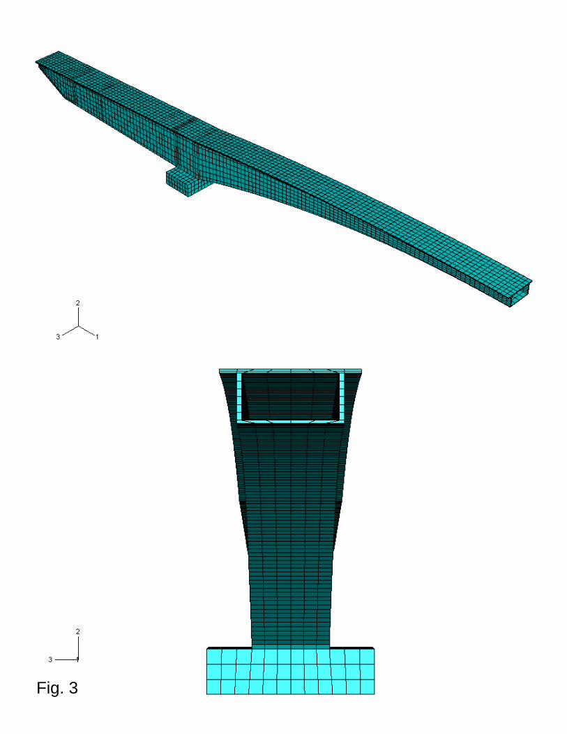
Fig. 3

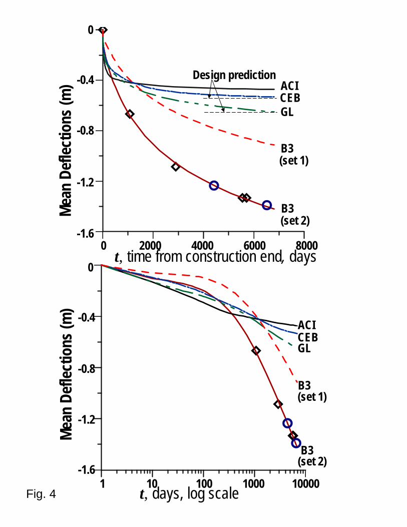
Fig. 4

t, time from construction end, days0

Mean

Def

lectio

ns (m

)

0

0 2000 4000 6000 8000

-0.4

-0.8

-1.2

-1.6

ACICEBGL

B3

(set 2)

(set 1)

B3

Design predictionMe

an D

eflec

tions

(m)

1 10 100 1000 10000t, days, log scale

-0.4

-0.8

-1.2

-1.6 (set 2)

CEBGL

(set 1)

ACI

B3

B3

Fig. 5

Mean

Def

lectio

ns (m

)

t, time from construction end, days0

B3

Mean

Def

lectio

ns (m

)

0

0 20000 40000 60000

-0.5

-1.0

-1.5

-2.0

-2.5

ACICEB

GL

(set 1)

(set 2)B3

1 10 100 1000 10000 100000

-0.5

-1.0

-1.5

-2.0

-2.5

ACICEB

GL

t, days, log scale

(set 1)B3

(set 2)B3

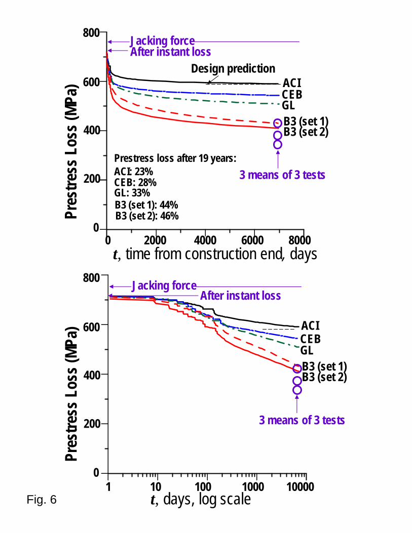
Fig. 6

Pres

tress

Loss

(MPa

)

B3 (set 2)

Pres

tress

Loss

(MPa

)

800

0 2000 4000 6000 8000

600

400

200

0

ACICEBGLB3 (set 1)

3 means of 3 tests

t, time from construction end, days

Design predictionAfter instant loss

Prestress loss after 19 years:ACI: 23%CEB: 28%GL: 33%B3 (set 1): 44%B3 (set 2): 46%

Jacking force

B3 (set 2)

800

600

400

200

01 10 100 1000 10000

t, days, log scale

3 means of 3 tests

Jacking forceAfter instant loss

ACICEBGLB3 (set 1)

Fig. 7

Mean

Def

lectio

ns (m

)

t, time from construction end, days

0

0 2000 4000 6000 8000

-0.4

-0.8

-1.2

-1.6

No shrinkage, no drying creep

Uniform creep and shrinkage

No drying creep

over cross section

(basic creep only)

1 10 100 1000 10000

0

-0.4

-0.8

-1.2

-1.6

t, days, log scale

Mean

Def

lectio

ns (m

)

No shrinkage,no drying creep

Uniform creep and shrinkageover cross section

No drying creep

0 2000 4000 6000 8000

No drying creep

1 10 100 1000 10000

800

640

480

320

160

0

No drying creep

Fig. 8

Pres

tress

Loss

(MPa

)Pr

estre

ssLo

ss (M

Pa)

t, days, log scale

t, time from construction end, days

800

640

480

320

160

0

Uniform creep and shrinkageover cross section

No shrinkage, no drying creep(basic creep only)

No shrinkage,no drying creep

Uniform creep and shrinkageover cross section

Defle

ctio

ns (m

)

Fig. 9

0

Defle

ctio

ns (m

)

0 2000 4000 6000 8000t, time from construction end, days

0

-0.4

-0.8

-1.2

-1.6

-2.0

1 10 100 1000 10000t, days, log scale

-0.4

-0.8

-1.2

-1.6

-2.0

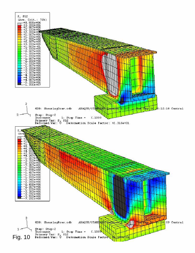
Fig. 10

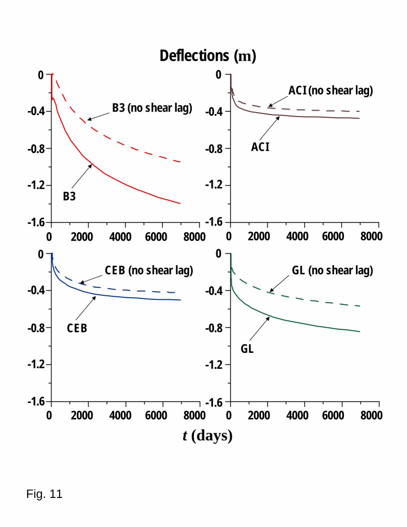
B3 (no shear lag)

B3

ACI (no shear lag)

ACI

CEB (no shear lag)

CEB

GL (no shear lag)

GL

Fig. 11

0

0 2000 4000 6000 8000

-0.4

-0.8

-1.2

-1.6

Deflections (m)0

-0.4

-0.8

-1.2

-1.60 2000 4000 6000 8000

0 2000 4000 6000 8000 0 2000 4000 6000 8000

0

-0.4

-0.8

-1.2

-1.6

0

-0.4

-0.8

-1.2

-1.6

t (days)

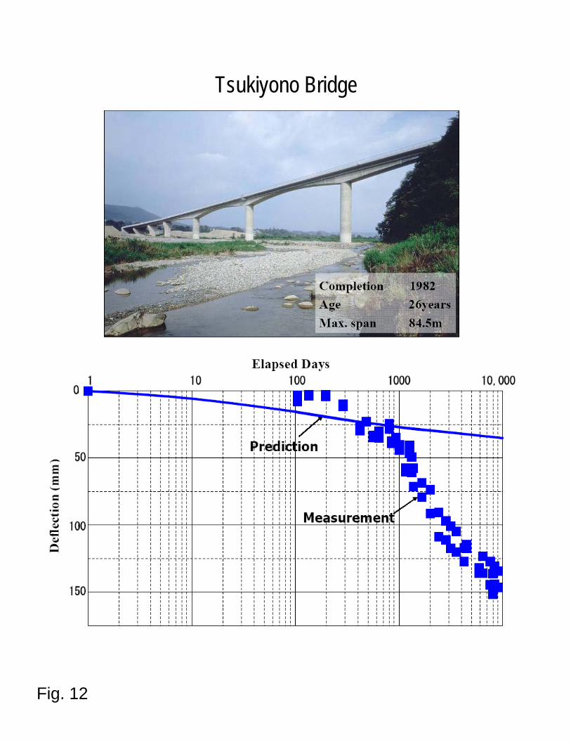
Tsukiyono Bridge

Fig. 12

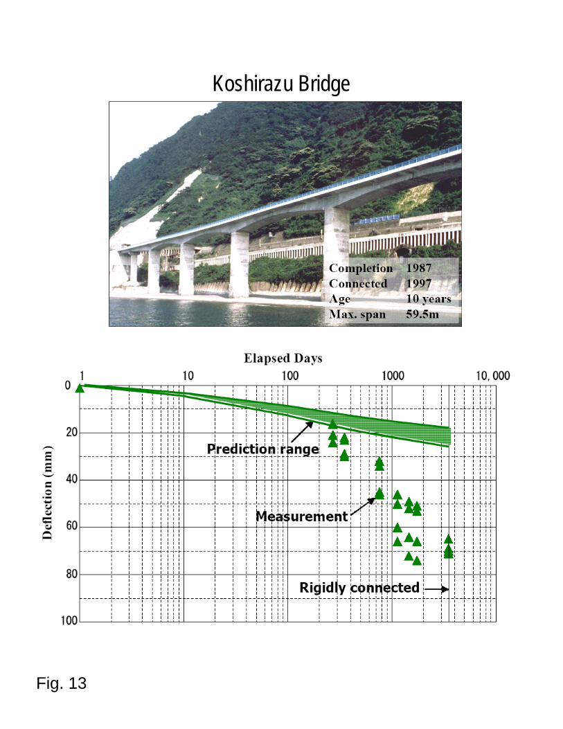
Koshirazu Bridge

Fig. 13

Konaru Bridge

Fig. 14

Urado Bridge

Fig. 15