explicit option pricing formula for a mean-reverting asset in
TRANSCRIPT

Explicit Option Pricing Formula
for a Mean-Reverting Asset in
Energy Markets
Anatoliy SwishchukMathematical & Computational
Finance LabDept of Math & Stat, University
of Calgary, Calgary, AB, CanadaQMF 2007 Conference
Sydney, AustraliaDecember 12-15, 2007
This research is supported by MITACS and NSERC

Outline
• Mean-Reverting Models (MRM): Deterministic vs. Stochastic
• MRM in Finance Markets: Variances or Volatilities (Not Asset Prices)
• MRM in Energy Markets: Asset Prices
• Change of Time Method (CTM)
• Mean-Reverting Model (MRM)
• Option Pricing Formula
• Drawback of One-Factor Models
• Future Work

Motivations for the Work
• Paper: Javaheri, Wilmott and Haug (2002)
”GARCH and Volatility Swaps”, Wilmott
Magazine, Jan Issue (they applied PDE
approach to find a volatility swap for MRM and
asked about the possible option pricing formula
• Paper: Bos, Ware and Pavlov (2002) “On a
Semi-Spectral Method for Pricing an Option on a
Mean-Reverting Asset”, Quantit. Finance J.
(PDE approach, semi-spectral method to
calculate numerically the solution)

Wilmott, Javaheri & Haug (2002)
Model
• Wilmott, Javaheri & Haug (GARCH and Volatility Swaps, Wilmott Magazine, 2002)-volatility swap for
-continuous-time GARCH(1,1) model

M. Yor’s Results
• M. Yor On some exponential functions of
Brownian motion, Adv. In Applied Probab., v. 24,
No. 3, (1992), 509-531-started the research for
the integral of an exponential Brownian motion
• H. Matsumoto, M. Yor Exponential Functionals
of Brownian motion, I: Probability laws at fixed
time, Probability Surveys, v. 2 (2005), 312-347-
there is still no closed form probability density
function, while the best result is a function with a
double integral.

Mean-Reversion Effect
• Guitar String Analogy: if we pluck the guitar string, the string will revert to its place of equilibrium
• To measure how quickly this reversion back to the equilibrium location would happen we had to pluck the string
• Similarly, the only way to measure mean reversion is when the variances of asset prices in financial markets and asset prices in energy markets get plucked away from their non-event levels and we observe them go back to more or less the levels they started from

The Mean-Reverting Deterministic Process

Mean-Reverting Plot (a=4.6,L=2.5)

Meaning of Mean-Reverting Parameter
• The greater the mean-reverting parameter
value, a, the greater is the pull back to the
equilibrium level
• For a daily variable change, the change in time,
dt, in annualized terms is given by 1/365
• If a=365, the mean reversion would act so
quickly as to bring the variable back to its
equilibrium within a single day
• The value of 365/a gives us an idea of how
quickly the variable takes to get back to the
equilibrium-in days

Mean-Reverting Stochastic Process

Mean-Reverting Models in Financial
Markets
• Stock (asset) Prices follow
geometric Brownian motion
• The Variance of Stock Price
follows Mean-Reverting Models
• Example: Heston Model

Mean-Reverting Models in
Energy Markets
• Asset Prices follow Mean-Reverting Stochastic Processes
• Example: Continuous-Time GARCH Model (or Pilipovic One-Factor Model)

Mean-Reverting Models in Energy
Markets

Change of Time: Definition and Examples
• Change of Time-change time from t to a non-negative process T(t) with non-decreasing sample paths
• Example1 (Subordinator): X(t) and T(t)>0 are some processes, then X(T(t)) is subordinated to X(t); T(t) is change of time
• Example 2 (Time-Changed Brownian Motion): M(t)=B(T(t)), B(t)-Brownian motion
• Example 3 (Product Process):

Time-Changed Brownian Motion by Bochner
• Bochner (1949) (‘Diffusion Equation and Stochastic Process’, Proc. N.A.S. USA, v. 35)-introduced the notion of change of time (CT) (time-changed Brownian motion)
• Bochner (1955) (‘Harmonic Analysis and the Theory of Probability’, UCLA Press, 176)-further development of CT

Change of Time: First Intro into Financial Economics
• Clark (1973) (‘A
‘Subordinated Stochastic
Process Model with Fixed Variance for Speculative
Prices’, Econometrica, 41, 135-156)-introduced
Bochner’s (1949) time-
changed Brownian motion into financial
economics:
• He wrote down a model for the log-price M as
M(t)=B(T(t)),
• where B(t) is Brownian
motion, T(t) is time-
change (B and T are independent)

Change of Time: Short History. I.
• Feller (1966) (‘An Introduction to Probability
Theory’, vol. II, NY: Wiley)-introduced subordinated
processes X(T(t)) with Markov process X(t) and T(t) as a process with independent increments (i.e., Poisson
process); T(t) was called randomized operational time
• Johnson (1979) (‘Option Pricing When the
Variance Rate is Changing’, working paper, UCLA)-introduced time-changed SVM in continuous time
• Johnson & Shanno (1987) (‘Option Pricing
When the Variance is Changing’, J. of Finan. & Quantit.
Analysis, 22, 143-151)-studied the pricing of options
using time-changing SVM

Change of Time: Short History. II.
• Ikeda & Watanabe (1981) (‘SDEs and Diffusion Processes’, North-Holland Publ. Co)-introduced and studied CTM for the solution of SDEs
• Barndorff-Nielsen, Nicolato & Shephard (2003) (‘Some recent development in stochastic volatility modelling’)-review and put in context some of their recent work on stochastic volatility (SV) modelling, including the relationship between subordination and SV (random time-chronometer)
• Carr, Geman, Madan & Yor (2003) (‘SV for Levy Processes’, mathematical Finance, vol.13)-used subordinated processes to construct SV for Levy Processes (T(t)-business time)

CT and Embedding Problem
• Embedding Problem was first terated by Skorokhod(1965)-sum of any sequence of i.r.v. with mean zero and
finite variation could be embedded in Brownian motion
(BM) using stopping time
• Dambis (1965) and Dubis and Schwartz (1965)-every
continuous martingale could be time-changed BM
• Huff (1969)-every processes of pathwise bounded
variation could be embedded in BM
• Monroe (1972)-every right continuous martingale could
be embedded in a BM
• Monroe (1978)-local martingale can be embedded in BM

Change of Time:
Simplest (Martingale) Case

Change of Time:
Ito Integral’s Case

Change of Time: SDE’s Case

Geometric Brownian Motion SVM

Change of Time Method

Connection between phi_t and phi_t^(-1)

Solution for GBM Equation
Using Change of Time

Explicit Expression for

Mean-Reverting SV Model

Solution of MRM by CTM

Explicit Expression for

Explicit Expression for

Comparison: Solution of GBM & MRM
-GBM
-MRM

Explicit Expression for S(t)
where

Properties of

Properties of

Properties of eta(t)

Properties of Eta(t). II.

Mean Value of MRM S(t)

Dependence of ES(t) on T

Dependence of ES(t) on S_0 and T

Variance for S(t)

Dependence of Variance of S(t) on S_0 and T

Dependence of Volatility of S(t) on S_0 and T

European Call Option for MRM.I.
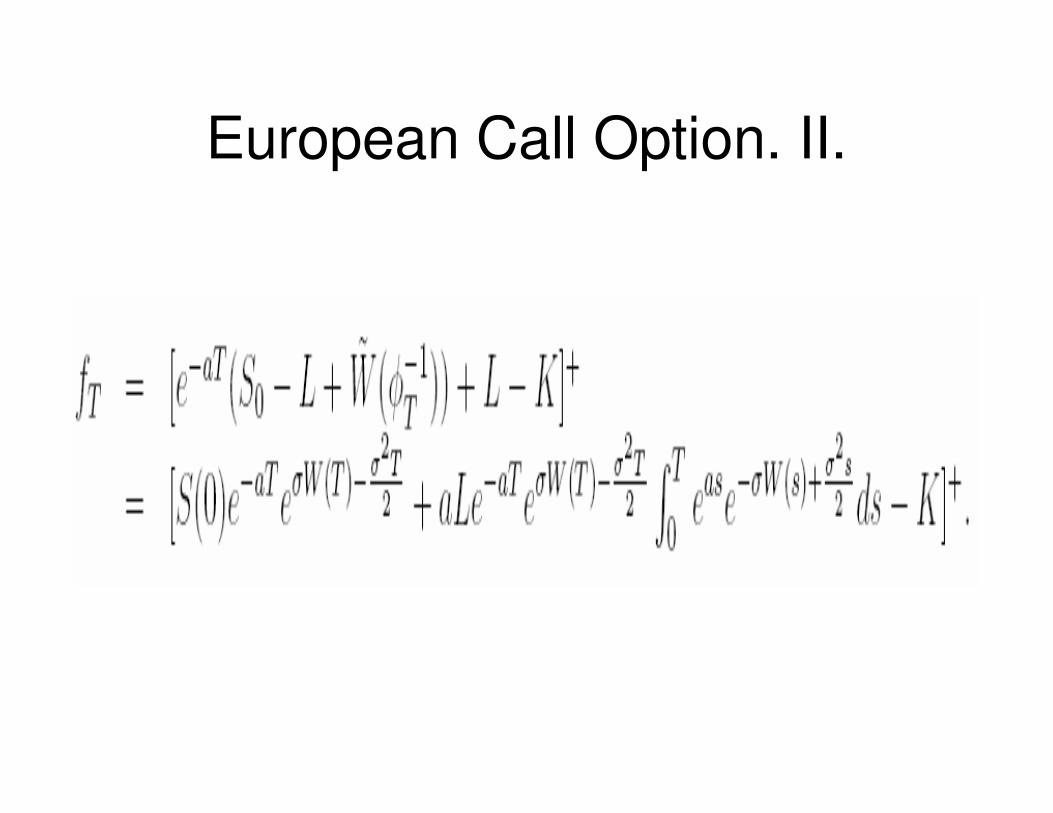
European Call Option. II.

Expression for C_T in the case of
MRM
C_T=BS(T)+A(T)

Expression for C_T=BS(T)+A(T).II.

Expression for BS(T)

Expression for y_0 for MRM

Expression for A(T).I.

Moment generating) function of
Eta(T)
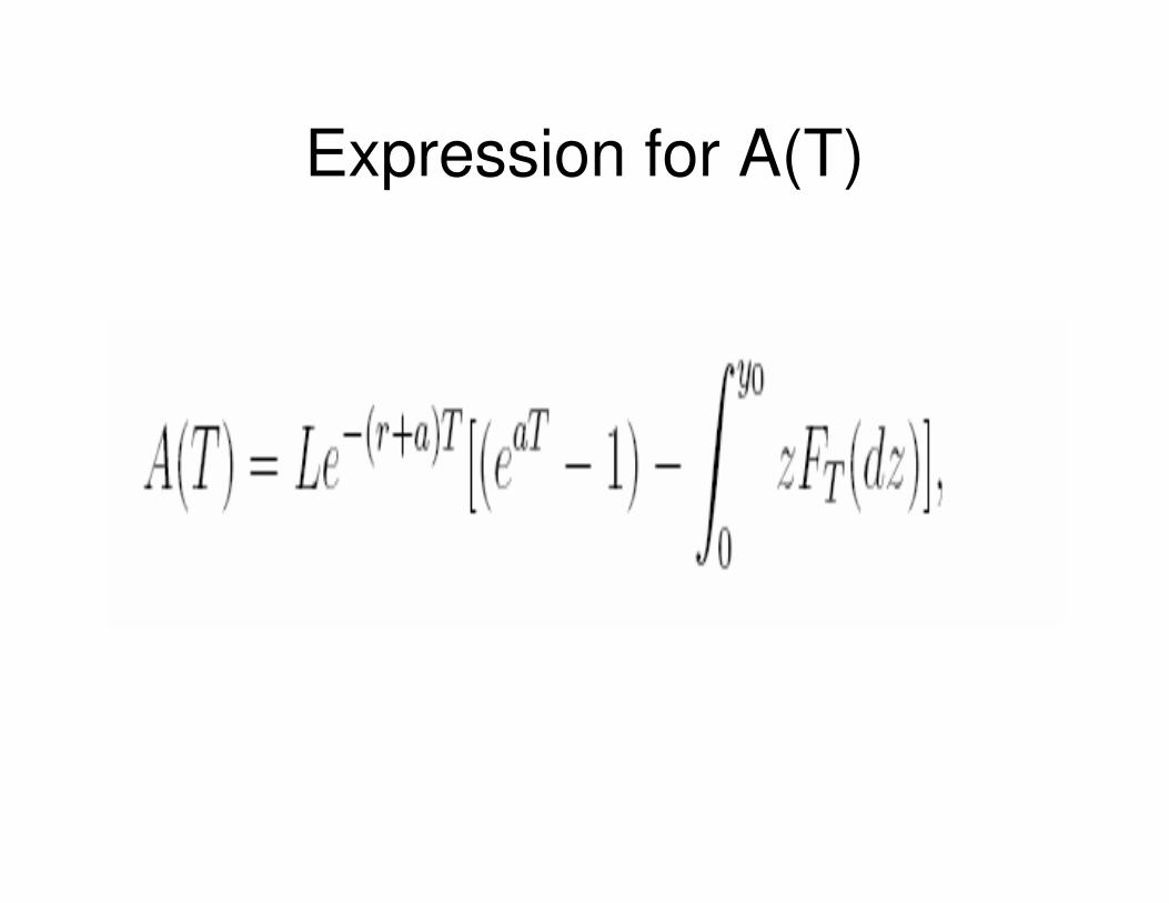
Expression for A(T)

European Call Option for MRM
(Explicit Formula)

European Call Option for MRM in Risk-Neutral
World


Dependence of C_T on T

Comparison of Three Solutions
• Heston Model
• Mean-Reverting Model
• Black-Scholes Model
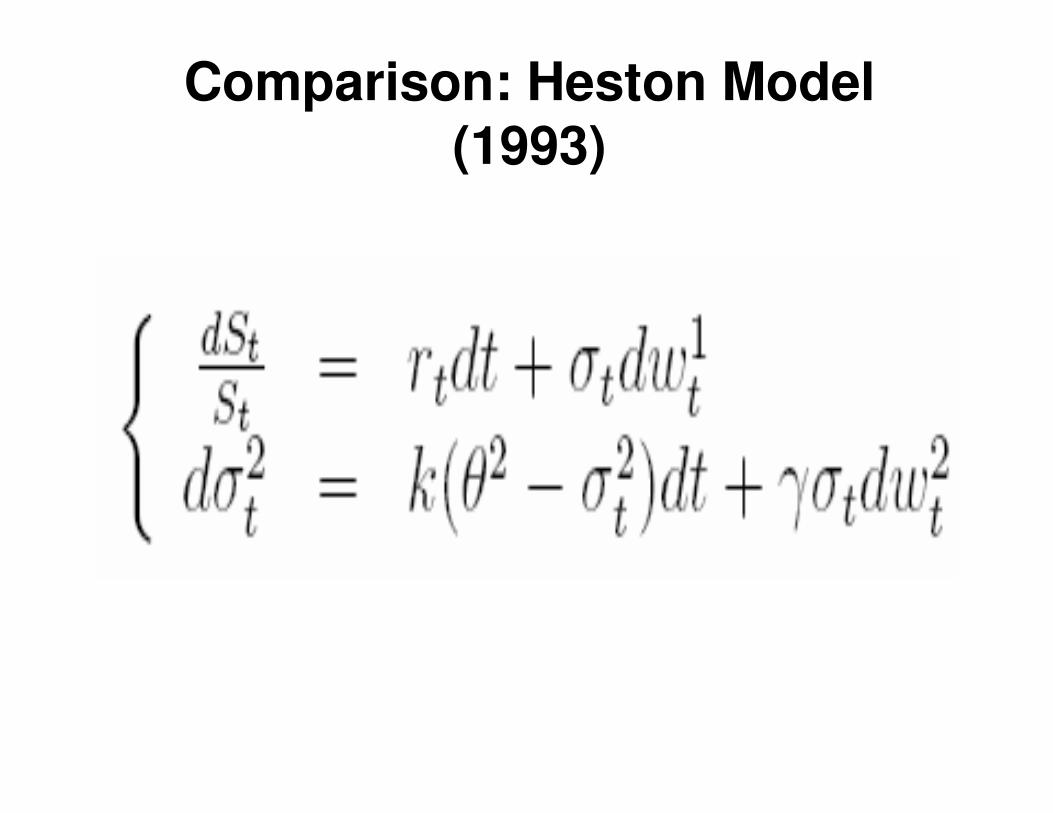
Comparison: Heston Model
(1993)

Explicit Solution for CIR Process: CTM

Comparison: Solutions to the Three
Models
-GBM
-MRM
-Heston model

Summary
-martingale
-martingale
-sum of two martingales
1.
2.
3.
GBM Model
Mean-Reverting Model
Heston Model

Problem
-explicit expression ?
We know all the moments at this moment, though
To calculate an option price for Heston model, for example

Drawback of One-Factor Mean-
Reverting Models
• The long-term mean L remains fixed over time: needs to be recalibrated on a continuous basis in order to ensure that the resulting curves are marked to market
• The biggest drawback is in option pricing: results in a model-implied volatility term structure that has the volatilities going to zero as expiration time increases (spot volatilities have to be increased to non-intuitive levels so that the long term options do not lose all the volatility value-as in the marketplace they certainly do not)

Future Work
• Change of Time
Method for Two-
Factor
Continuous-Time
GARCH Model

The End
Thank You for Your
Attention and Time!
http://wwww.math.ucalgary.ca/~aswish/