exploiting prior knowledge and latent variable representations … · 2015-12-22 · exploiting...
TRANSCRIPT
Exploiting Prior Knowledge and Latent
Variable Representations for the
Statistical Modeling and Probabilistic
Querying of Large Knowledge Graphs
Denis Krompaß
Munchen 2015

Exploiting Prior Knowledge and Latent
Variable Representations for the
Statistical Modeling and Probabilistic
Querying of Large Knowledge Graphs
Denis Krompaß
Dissertation
an der Fakultat fur Mathematik, Informatik und Statistik
der Ludwig–Maximilians–Universitat
Munchen
vorgelegt von
Denis Krompaß
aus Passau
Munchen, den 24.09.2015

Erstgutachter: Prof. Dr. Volker Tresp
Zweitgutachter: Prof. Dr. Steffen Staab
Tag der mundlichen Prufung: 20.11.2015
Eidesstattliche Versicherung(Siehe Promotionsordnung vom 12.07.11, §8, Abs. 2 Pkt. .5.)
Hiermit erklare ich an Eidesstatt, dass die Dissertation von mir
selbststandig, ohne unerlaubte Beihilfe angefertigt ist.
Denis Krompaß
- - - - - - - - - - - - - - - - - - - - - - - - - - - - - - - - - - - - - - - - - - - - - - - - - - - - - - - - - - - - - - - - - - - - - - - - - - - - -
Name, Vorname
Ort, Datum Unterschrift Doktorand
Formular 3.2

Acknowledgements
During the last years, many people contributed to the successful completion of my PhD.
First of all, I want to thank my supervisor at Siemens and the Ludwig Maximilian Uni-
versity of Munich, Prof. Dr. Volker Tresp. To me, Volker is not just a supervisor but
a mentor who positively influenced my research and my personal development with his
experience and guidance. There has been no time, where he was not open for discussions
on various topics and ideas and his valuable inputs often helped me to drive my research
on these topics in the right directions. I further thank Dr. Matthias Schubert with whom I
did my first real steps in machine learning during my master thesis. He also recommended
Volker as a supervisor for my PhD and introduced me to him. I also want to thank Michal
Skubacz, Research Group Head of Knowledge Modeling and Retrieval, who funded my
PhD, conference trips, rental of cloud services and gave me the possibility to continue my
career in his group at Siemens. I am also very grateful to Prof. Steffen Staab to act as
second examiner of my thesis work.
Special thanks goes to Maximilian Nickel whose research inspired my own work to
a large extent. I also had the pleasure to work with Xueyan Jiang, Cristobal Esteban,
Stephan Baier, Yinchong Yang, Sebnem Rusitschka and Sigurd Spieckermann and thank
them for a great working atmosphere and the sometimes long and constructive discussions.
In this regard, special thanks to Sigurd Spieckermann for in depth discussions on various
topics related to machine learning and for introducing me to Theano. Fortunately, we
will have the opportunity to continue working together in the near future as colleagues at
Siemens Corporate Technology in the research group Knowledge Modeling and Retrieval.
I especially thank my family for supporting me over all these years. To my brother
Daniel who introduced me to mathematics at the age of 5. My parents, Bertin and Marietta
who have always believed in and supported my career efforts even in very dificult times. To

viii Acknowledgements
Oma and OnkelP to which I could always turn for any matter or short and very relaxing
vacations in the “family headquarter”. My deep gratitude goes to Steffi who has always
supported me with her outstanding language and cooking skills. I also thank her for
introducing me to the many great things I was not aware of and for definitely broadening
my horizon in many aspects. Finally, I want to thank “den Jungs” for what I am sure, they
are aware of. (If not, then I will be happy to explain myself on the next annual meeting.)
Contents
1 Introduction 1
1.1 Learning in the Semantic Web . . . . . . . . . . . . . . . . . . . . . . . . . 4
1.2 Learning in Knowledge Graphs . . . . . . . . . . . . . . . . . . . . . . . . 4
1.3 Contributions of this Work . . . . . . . . . . . . . . . . . . . . . . . . . . . 6
2 Knowledge Graphs 9
2.1 Knowledge-Graphs are RDF-Triplestores . . . . . . . . . . . . . . . . . . . 12
2.1.1 RDF-Triple Structure . . . . . . . . . . . . . . . . . . . . . . . . . . 13
2.1.2 Schema Concepts . . . . . . . . . . . . . . . . . . . . . . . . . . . . 14
2.1.3 Knowledge Retrieval in Knowledge Graphs . . . . . . . . . . . . . . 16
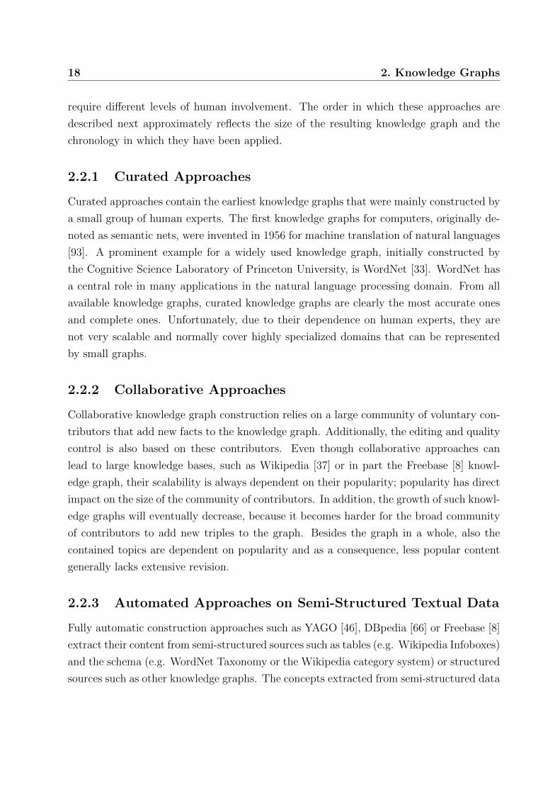
2.2 Knowledge Graph Construction . . . . . . . . . . . . . . . . . . . . . . . . 17
2.2.1 Curated Approaches . . . . . . . . . . . . . . . . . . . . . . . . . . 18
2.2.2 Collaborative Approaches . . . . . . . . . . . . . . . . . . . . . . . 18
2.2.3 Automated Approaches on Semi-Structured Textual Data . . . . . . 18
2.2.4 Automated Approaches on Unstructured Textual Data . . . . . . . 19
2.3 Popular Knowledge Graphs . . . . . . . . . . . . . . . . . . . . . . . . . . 21
2.3.1 DBpedia . . . . . . . . . . . . . . . . . . . . . . . . . . . . . . . . . 21
2.3.2 Freebase . . . . . . . . . . . . . . . . . . . . . . . . . . . . . . . . . 22
2.3.3 YAGO . . . . . . . . . . . . . . . . . . . . . . . . . . . . . . . . . . 23
2.4 Deficiencies in Today’s Knowledge Graph Data . . . . . . . . . . . . . . . . 24
3 Representation Learning in Knowledge Graphs 27
3.1 Representation Learning . . . . . . . . . . . . . . . . . . . . . . . . . . . . 27
3.2 Relational Learning . . . . . . . . . . . . . . . . . . . . . . . . . . . . . . . 30
x CONTENTS
3.3 Statistical Modeling of Knowledge Graphs with Latent Variable Models . . 32
3.3.1 Notation . . . . . . . . . . . . . . . . . . . . . . . . . . . . . . . . . 33
3.3.2 RESCAL . . . . . . . . . . . . . . . . . . . . . . . . . . . . . . . . 33
3.3.3 Translational Embeddings . . . . . . . . . . . . . . . . . . . . . . . 34
3.3.4 Google Knowledge-Vault Neural-Network . . . . . . . . . . . . . . . 35
4 Applying Latent Variable Models to Large Knowledge Graphs 37
4.1 Latent Variable Model Complexity in Large Knowledge Graphs . . . . . . 38
4.2 Simulating Large Scale Conditions . . . . . . . . . . . . . . . . . . . . . . . 39
4.2.1 Data Sets . . . . . . . . . . . . . . . . . . . . . . . . . . . . . . . . 40
4.2.2 Evaluation Procedure . . . . . . . . . . . . . . . . . . . . . . . . . . 42
4.2.3 Implementation and Model Training Details . . . . . . . . . . . . . 43
4.3 Experimental Results . . . . . . . . . . . . . . . . . . . . . . . . . . . . . . 44
4.3.1 Link-Prediction Quality – TransE has Leading Performance . . . . 44
4.3.2 Optimization Time – RESCAL is Superior to Other Methods . . . . 46
4.4 Related Work . . . . . . . . . . . . . . . . . . . . . . . . . . . . . . . . . . 47
4.5 Conclusion . . . . . . . . . . . . . . . . . . . . . . . . . . . . . . . . . . . . 48
5 Exploiting Prior Knowledge On Relation-Type Semantics 51
5.1 Type-Constrained Alternating Least-Squares for RESCAL . . . . . . . . . 52
5.1.1 Additional Notation . . . . . . . . . . . . . . . . . . . . . . . . . . 56
5.1.2 Integrating Type-Constraints into RESCAL . . . . . . . . . . . . . 57
5.1.3 Relation to Other Factorizations . . . . . . . . . . . . . . . . . . . . 61
5.1.4 Testing the Integration of Type-Constraints in RESCAL . . . . . . 61
5.1.5 Conclusion . . . . . . . . . . . . . . . . . . . . . . . . . . . . . . . . 65
5.2 Type-Constrained Stochastic Gradient Descent . . . . . . . . . . . . . . . . 65
5.2.1 Type-Constrained Triple Corruption in SGD . . . . . . . . . . . . . 66
5.3 A Local Closed-World Assumption for Modeling Knowledge Graphs . . . . 67
5.3.1 Entity Grouping for RESCAL under a Local Closed-World Assumption 69
5.3.2 Link-Prediction in DBpedia with RESCAL . . . . . . . . . . . . . . 70
5.3.3 Conclusion . . . . . . . . . . . . . . . . . . . . . . . . . . . . . . . . 71
5.4 Experiments – Prior Knowledge on Relation-Types is Important for Latent
Variable Models . . . . . . . . . . . . . . . . . . . . . . . . . . . . . . . . . 72
5.4.1 Type-Constraints are Essential . . . . . . . . . . . . . . . . . . . . 74
5.4.2 Local Closed-World Assumption – Simple but Powerful . . . . . . . 76

CONTENTS xi
5.5 Related Work . . . . . . . . . . . . . . . . . . . . . . . . . . . . . . . . . . 77
5.6 Conclusion . . . . . . . . . . . . . . . . . . . . . . . . . . . . . . . . . . . . 78
6 Ensemble Solutions for Representation Learning in Knowledge Graphs 79
6.1 Studying Complementary Effects between TransE, RESCAL and mwNN . 80
6.2 Experimental Setup . . . . . . . . . . . . . . . . . . . . . . . . . . . . . . . 82
6.3 Experiments – TransE, RESCAL and mwNN Learn Complementary Aspects
in Knowledge Graphs . . . . . . . . . . . . . . . . . . . . . . . . . . . . . . 82
6.3.1 Type-Constrained Ensembles . . . . . . . . . . . . . . . . . . . . . 83
6.3.2 Ensembles under a Local Closed-World Assumption . . . . . . . . . 84
6.4 Related Work . . . . . . . . . . . . . . . . . . . . . . . . . . . . . . . . . . 85
6.5 Conclusion . . . . . . . . . . . . . . . . . . . . . . . . . . . . . . . . . . . . 86
7 Querying Statistically Modeled Knowledge Graphs 87
7.1 Exploiting Uncertainty in Knowledge Graphs . . . . . . . . . . . . . . . . . 89
7.1.1 Notation . . . . . . . . . . . . . . . . . . . . . . . . . . . . . . . . . 91
7.1.2 Probabilistic Databases . . . . . . . . . . . . . . . . . . . . . . . . . 92
7.1.3 Querying in Probabilistic Databases . . . . . . . . . . . . . . . . . . 95
7.2 Exploiting Latent Variable Models for Querying . . . . . . . . . . . . . . . 99
7.2.1 Learning Compound Relations with RESCAL . . . . . . . . . . . . 102
7.2.2 Learning Compound Relations with TransE and mwNN . . . . . . . 103
7.2.3 Numerical Advantage of Learned Compound Relation-Types . . . . 105
7.3 Evaluating the Learned Compound Relations . . . . . . . . . . . . . . . . . 106
7.3.1 Experimental Setup . . . . . . . . . . . . . . . . . . . . . . . . . . . 106
7.3.2 Compound Relations are of Good Quality . . . . . . . . . . . . . . 107
7.4 Querying Factorized DBpedia-Music . . . . . . . . . . . . . . . . . . . . . 109
7.4.1 DBpedia-Music . . . . . . . . . . . . . . . . . . . . . . . . . . . . . 109
7.4.2 Experimental Setup . . . . . . . . . . . . . . . . . . . . . . . . . . . 109
7.4.3 Queries Used for Evaluation . . . . . . . . . . . . . . . . . . . . . . 111
7.4.4 Learned Compound Relations Improve Quality of Answers . . . . . 113
7.4.5 Learned Compound Relations Decrease Query Evaluation Time . . 119
7.5 Related Work . . . . . . . . . . . . . . . . . . . . . . . . . . . . . . . . . . 120
7.6 Conclusion . . . . . . . . . . . . . . . . . . . . . . . . . . . . . . . . . . . . 122

xii Contents
8 Conclusion 123
8.1 Summary . . . . . . . . . . . . . . . . . . . . . . . . . . . . . . . . . . . . 123
8.2 Future Directions and Applications . . . . . . . . . . . . . . . . . . . . . . 126
List of Figures
2.1 Result of Google Query “Angela Kasner” . . . . . . . . . . . . . . . . . . . 10
2.2 Comparison of smart assistants . . . . . . . . . . . . . . . . . . . . . . . . 11
2.3 Illustration of ontology described in Table 2.3 . . . . . . . . . . . . . . . . 15
2.4 Graph representation of facts from Table 2.4 . . . . . . . . . . . . . . . . . 16
2.5 Illustration of automatic knowledge graph completion based on unstructured
textual data . . . . . . . . . . . . . . . . . . . . . . . . . . . . . . . . . . . 20
2.6 Distribution of facts per entity in DBpedia on a log scale. . . . . . . . . . . 24
5.1 Schematic of factorizing knowledge-graph data with RESCAL with and
without prior knowledge on type-constraints. . . . . . . . . . . . . . . . . . 53
5.2 Exploiting type-constraints in RESCAL: Results on the Cora and DBpedia-
Music data sets . . . . . . . . . . . . . . . . . . . . . . . . . . . . . . . . . 63
5.3 Illustration of how the local closed-world assumption . . . . . . . . . . . . 68
5.4 Exploiting the local closed-world assumption in RESCAL: Results on the
DBpedia data sets . . . . . . . . . . . . . . . . . . . . . . . . . . . . . . . 70
7.1 Illustration of a knowledge graph before and after transforming and filtering
the extracted triples based on uncertainty . . . . . . . . . . . . . . . . . . 90
7.2 Evaluation of learned compound relations: AUPRC results on the Nations
data set . . . . . . . . . . . . . . . . . . . . . . . . . . . . . . . . . . . . . 108
7.3 Evaluation of learned compound relations: AUPRC results on the UMLS
data set . . . . . . . . . . . . . . . . . . . . . . . . . . . . . . . . . . . . . 108
7.4 Query evaluation times in seconds for queries Q1(x), Q2(x) and Q3(x) . . . 119

xiv List of Figures
List of Tables
2.1 Abbreviations for URIs . . . . . . . . . . . . . . . . . . . . . . . . . . . . . 12
2.2 Example of defining type-constraints with RDFS . . . . . . . . . . . . . . . 15
2.3 Sample triples from the DBpedia ontology . . . . . . . . . . . . . . . . . . 15
2.4 Example triples from DBpedia on Billy Gibbons and Nickelback . . . . . . 16
4.1 Parameter complexity of latent variable models used in this work . . . . . 38
4.2 Details on Freebase-150k, DBpedia-Music and YAGOc-195k data sets . . . 40
4.3 AUPRC and AUROC results of RESCAL, TransE and mwNN on the Freebase-
150k data set . . . . . . . . . . . . . . . . . . . . . . . . . . . . . . . . . . 44
4.4 AUPRC and AUROC results of RESCAL, TransE and mwNN on the DBpedia-
Music data set . . . . . . . . . . . . . . . . . . . . . . . . . . . . . . . . . . 45
4.5 AUPRC and AUROC results of RESCAL, TransE and mwNN on the YAGOc-
195k data set . . . . . . . . . . . . . . . . . . . . . . . . . . . . . . . . . . 46
5.1 Details on Cora and DBpedia-Music data sets used in the experiments. . . 61
5.2 Comparison of AUPRC and AUROC result for RESCAL with and without
exploiting prior knowledge on relations types . . . . . . . . . . . . . . . . . 73
5.3 Comparison of AUPRC and AUROC result for TransE with and without
exploiting prior knowledge on relations types . . . . . . . . . . . . . . . . . 74
5.4 Comparison of AUPRC and AUROC result for mwNN with and without
exploiting prior knowledge on relations types . . . . . . . . . . . . . . . . . 75
6.1 AUPRC results on Freebase-150k, DBpedia-Music and YAGOc-195, exploit-
ing type-constraints in the ensembles . . . . . . . . . . . . . . . . . . . . . 83
xvi Abstract
6.2 AUPRC results on Freebase-150k, DBpedia-Music and YAGOc-195, exploit-
ing the Local Closed-World Assumption in the ensembles . . . . . . . . . . 85
7.1 Probabilistic conditional table consisting of the the relation-type knows from
Figure 7.1a . . . . . . . . . . . . . . . . . . . . . . . . . . . . . . . . . . . 93
7.2 Probabilistic conditional table consisting of the relation-type friendOf from
Figure 7.1a . . . . . . . . . . . . . . . . . . . . . . . . . . . . . . . . . . . 95
7.3 Probabilistic conditional table consisting of the the relation-type bornIn . 98
7.4 Details on the Nations, UMLS and DBpedia-Music data sets used in the
experiments . . . . . . . . . . . . . . . . . . . . . . . . . . . . . . . . . . . 106
7.5 AUPRC, AUROC and LogLoss scores for evaluating Q1(x) on DBpedia-Music114
7.6 AUPRC, AUROC and LogLoss scores for evaluating Q2(x) on DBpedia-Music116
7.7 Top 25 ranked answers produced by evaluating query Q2(x) with learned
compound relations . . . . . . . . . . . . . . . . . . . . . . . . . . . . . . . 117
7.8 AUPRC, AUROC and LogLoss scores for evaluating Q3(x) on DBpedia-Music118
Abstract
Large knowledge graphs increasingly add great value to various applications that require
machines to recognize and understand queries and their semantics, as in search or question
answering systems. These applications include Google search, Bing search, IBM’s Wat-
son, but also smart mobile assistants as Apple’s Siri, Google Now or Microsoft’s Cortana.
Popular knowledge graphs like DBpedia, YAGO or Freebase store a broad range of facts
about the world, to a large extent derived from Wikipedia, currently the biggest web en-
cyclopedia. In addition to these freely accessible open knowledge graphs, commercial ones
have also evolved including the well-known Google Knowledge Graph or Microsoft’s Satori.
Since incompleteness and veracity of knowledge graphs are known problems, the statistical
modeling of knowledge graphs has increasingly gained attention in recent years. Some
of the leading approaches are based on latent variable models which show both excellent
predictive performance and scalability. Latent variable models learn embedding represen-
tations of domain entities and relations (representation learning). From these embeddings,
priors for every possible fact in the knowledge graph are generated which can be exploited
for data cleansing, completion or as prior knowledge to support triple extraction from un-
structured textual data as successfully demonstrated by Google’s Knowledge-Vault project.
However, large knowledge graphs impose constraints on the complexity of the latent em-
beddings learned by these models. For graphs with millions of entities and thousands of
relation-types, latent variable models are required to exploit low dimensional embeddings
for entities and relation-types to be tractable when applied to these graphs.
The work described in this thesis extends the application of latent variable models for
large knowledge graphs in three important dimensions.
First, it is shown how the integration of ontological constraints on the domain and range
of relation-types enables latent variable models to exploit latent embeddings of reduced
xviii Abstract
complexity for modeling large knowledge graphs. The integration of this prior knowledge
into the models leads to a substantial increase both in predictive performance and scala-
bility with improvements of up to 77% in link-prediction tasks. Since manually designed
domain and range constraints can be absent or fuzzy, we also propose and study an al-
ternative approach based on a local closed-world assumption, which derives domain and
range constraints from observed data without the need of prior knowledge extracted from
the curated schema of the knowledge graph. We show that such an approach also leads to
similar significant improvements in modeling quality. Further, we demonstrate that these
two types of domain and range constraints are of general value to latent variable models
by integrating and evaluating them on the current state of the art of latent variable models
represented by RESCAL, Translational Embedding, and the neural network approach used
by the recently proposed Google Knowledge Vault system.
In the second part of the thesis it is shown that the just mentioned three approaches
all perform well, but do not share many commonalities in the way they model knowl-
edge graphs. These differences can be exploited in ensemble solutions which improve the
predictive performance even further.
The third part of the thesis concerns the efficient querying of the statistically mod-
eled knowledge graphs. This thesis interprets statistically modeled knowledge graphs as
probabilistic databases, where the latent variable models define a probability distribution
for triples. From this perspective, link-prediction is equivalent to querying ground triples
which is a standard functionality of the latent variable models. For more complex querying
that involves e.g. joins and projections, the theory on probabilistic databases provides eval-
uation rules. In this thesis it is shown how the intrinsic features of latent variable models
can be combined with the theory of probabilistic databases to realize efficient probabilistic
querying of the modeled graphs.
Zusammenfassung
Wissensgraphen spielen in vielen heutigen Anwendungen wie Websuche oder automatis-
chen Frage-Antwort-Systemen eine bedeutende Rolle. Dabei werden Maschinen von Wis-
sensgraphen darin unterstutzt, die Kernaspekte der Semantik von Benutzeranfragen zu
erkennen und zu verstehen. Prominente Beispiele, in denen die Integration von Wissens-
graphen einen beachtlichen Mehrwert geliefert hat, sind Googles und Microsofts Websuche
sowie IBMs Watson. Im mobilen Bereich sind vor allem auch diverse Assistenzsysteme wie
Google Now, Apple Siri und Microsoft Cortana nennenswert. Die wahrscheinlich bekan-
ntesten Wissensgraphen sind der kommerziell genutzte Google Knowledge Graph und Mi-
crosofts Satori, die vor allem die Websuche unterstutzen. Freebase, DBpedia und YAGO
gehoren zu den bekanntesten Beispielen fur Wissensgraphen, die einen freien Zugriff auf
ihre Daten erlauben. Diese Graphen haben gemeinsam, dass sie eine breite Sammlung
von Fakten speichern, die zu einem großen Teil von Wikipedia stammen, der momentan
großten verfugbaren Web-Enzyklopadie. Trotz des großen Mehrwerts, den diese Graphen
bereits heute erbringen, gibt es einige Aspekte, die zu Einschrankungen und Problemen
bei der Anwendung fuhren. Zu diesen Aspekten gehoren vor allem Unsicherheit und Un-
vollstandigkeit der gespeicherten Fakten. Statistisch motivierte Verfahren zur Modellierung
dieser Graphen stellen einen Ansatz dar um diese Probleme zu adressieren. Dabei haben
sich insbesondere Latent Variable Models, die zum Bereich des Reprasentations-Lernens
gehoren, als sehr erfolgversprechend erwiesen. Diese Modelle lernen latente Reprasenta-
tionen fur Entitaten und Relationen, aus denen Schlussfolgerungen uber die Richtigkeit
fur jede mogliche Relation zwischen Entitaten abgeleitet werden konnen. Diese Schlussfol-
gerungen konnen dazu benutzt werden bestehende Wissensgraphen aufzubereiten, zu ver-
vollstandigen oder sogar um die automatische Konstruktion von neuen Wissensgraphen
aus unstrukturierten Freitexten zu unterstutzen, wie es im kurzlich veroffentlichten Google
xx Zusammenfassung
Knowledge Vault Projekt demonstriert wurde.
Die Modellierung von sehr großen Wissensgraphen stellt eine zusatzliche Herausforderung
fur diese Modelle dar, da die Große des modellierten Graphen direkten Einfluss auf die
Komplexitat und damit auf die Trainingszeit der Modelle hat. Wissensgraphen mit Millio-
nen von Entitaten und Tausenden von unterschiedlichen Arten von Relationen erfordern
es, dass die Latent Variable Models mit niedrigdimensionalen latenten Reprasentationen
fur Entitaten und die verschiedenen Relationen auskommen mussen.
Diese Doktorarbeit erweitert die Anwendung von Latent Variable Models auf große
Wissensgraphen in Bezug auf drei wichtige Aspekte.
Erstens, die Integration von Vorwissen uber die Semantik von Relationen in Latent Vari-
able Models fuhrt dazu, dass die Graphen mit niedrigdimensionalen latenten Reprasentatio-
nen besser modelliert werden konnen. Dieses Vorwissen steht in Schema-basierten Wissens-
graphen oft zur Verfugung. Dabei konnten durch die Berucksichtigung dieses Vorwissens
erhebliche Verbesserungen von bis zu 77% bei der Vorhersage von neuen Verbindungen im
Graphen erzielt werden. Zusatzlich wird ein alternativer Ansatz vorgestellt, eine Annahme
der lokalen Weltabgeschlossenheit, der angewendet werden kann wenn Vorwissen uber die
Semantik von Relationen nicht verfugbar oder ungenau ist. Durch diese Annahme kann
die Semantik von Relationen auf Basis der vorhandenen Fakten im Graph abgeschatzt
werden und ist damit unabhangig von einem vorgegebenen Schema. Es wird gezeigt, dass
dieser Ansatz ebenfalls zu einer erheblichen Verbesserung in der Vorhersage-Qualitat fuhrt.
Ferner wird argumentiert, dass beide Arten des Vorwissens uber die Semantik von Relatio-
nen, zum Einen extrahiert aus dem Schema des Wissensgraphen, zum Anderen abgeleitet
von der Annahme der lokalen Weltabgeschlossenheit, generell essentiell fur Latent Variable
Models zur Modellierung von großen Wissensgraphen ist. Zu diesem Zweck werden beide
Arten von Vorwissen in drei Modelle, die den Stand der Technik reprasentieren integriert
und untersucht: die Latent Variable Models RESCAL, TransE und das neuronale Netz,
welches im Google Knowledge Vault Projekt verwendet wurde.
Die oben genannten drei Modelle haben durch Integration von Vorwissen eine gute
Vorhersage Qualitat, modellieren jedoch den Wissensgraphen auf sehr unterschiedliche Art
und Weise. Fur den zweiten Aspekt wird gezeigt, dass diese Unterschiede zwischen den
Modellen in Ensemble-Methoden ausgenutzt werden konnen um die Vorhersage Qualitat
weiter zu verbessern.
Der dritte und letzte Aspekt, der in dieser Arbeit beschrieben wird, behandelt die ef-
fiziente Abfrage von statistisch modellierten Wissensgraphen. Zu diesem Zweck wird der

Zusammenfassung xxi
statistisch modellierte Wissensgraph als probabilistische Datenbank interpretiert, wobei
das Latent Variable Model die Wahrscheinlichkeitsverteilung der reprasentierten Fakten
definiert. Ausgehend von dieser Interpretation kann die ubliche Vorhersage von neuen
Verbindungen im Graphen mit den Latent Variable Models als eine Abfrage dieser Daten-
bank nach einzelnen einfachen Fakten aufgefasst werden. Fur komplexere Abfragen, die
zum Beispiel Joins oder Projektionen beinhalten konnen, stellt die Theorie der proba-
bilistischen Datenbank Auswertungsregeln bereit. Es wird gezeigt, wie wesentliche Eigen-
schaften der Latent Variable Models mit der Theorie der probabilistischen Datenbanken
kombiniert werden konnen um das effiziente Abfragen der statistisch modellierten Wissens-
graphen zu ermoglichen.

xxii Zusammenfassung
Chapter 1Introduction
The rapidly growing Web of Data, e.g., as presented by the Semantic Web’s linked open
data cloud (LOD) [6], is providing an increasing amount of data in form of large triple
databases, also known as triple stores. The main vision of the Semantic Web is to create a
structured Web of knowledge from the content of the World Wide Web. The organization
of this structured knowledge can be distinguished in two different ways, by schema-free
or schema-based graph-based knowledge bases. In schema-free knowledge graphs open
information extraction techniques (OpenIE) [29, 30] identify entities and relations from text
documents and represent them by their surface names, that is the corresponding string from
the textual data. This approach has the advantage that no predefined vocabulary is needed,
but the entities and relation-types often lack proper disambiguation, e.g. the system might
not explicitly represent the knowledge that ”Angela Kasner” and ”Angela Merkel” refer to
the same real-world entity. In schema-based knowledge graphs on the other hand, one aims
to represent entities and relation-types by unique global identifiers. This representation
also stores the surface names of entities as literal entities, but in the best case all surface
names that refer to the same real-world entity are properly disambiguated through linking
them to the same unique global identifier. In Freebase [8] for example, ”Angela Kasner”
and ”Angela Merkel” both refer to the Freebase identifier /m/0jl0g. Additionally, all
entities and relation-types are predefined by a fixed vocabulary which is often semantically
enriched in not necessarily hierarchical ontologies. Through the semantics, entities become
real-world things like persons or cities that have various types of relationships and are often
enriched with a large amount of additional information that further describe them and
their meaning. The Freebase entity with identifier /m/0jl0g (Angela Merkel) for example
belongs to the class person and is the current chancellor of Germany, where chancellor is
2 1. Introduction
a governmental position. This kind of semantically rich description of real-world entities
adds great value to various applications such as web-search, question answering and relation
extraction. In these applications, entities and relation-types can be recognized by machines
and additional background knowledge can be acquired that better represents the intention
of the user. The Google Knowledge Graph is certainly the most famous example, where
such approach significantly improved the quality and user experience in web-search.
Today, hundreds of different knowledge graphs have emerged, which represent in part
domain specific (e.g. the Gene Ontology [2]), but also general purpose (e.g. Freebase)
knowledge. Besides academic efforts to construct large and extensive knowledge graphs
like Freebase, DBpedia [66], Nell [16] or YAGO [46], also commercially ones have evolved
including Google’s and Yahoo!’s Knowledge-Graph or Microsoft’s Satori. Based on au-
tomated knowledge extraction methods and partially also thanks to a large number of
volunteers that are contributing facts and perform quality control, some of the knowledge
graphs contain billions of facts about millions of entities, which are related by thousands
of different relation-types. Due to the effort of the linked open data initiative, entities have
been additionally interlinked between different knowledge graphs, allowing an easier inte-
gration of knowledge from different sources of the linked open data cloud. Especially the
possibility to combine different sources of information allows machines to consider more
diverse information and to better understand the notion of a given task, leading to im-
proved and new applications and services. Today, knowledge graphs power a various set of
commercial applications including well known search engines such as Google, Bing, Yahoo
or Facebooks’s Graph search, but also smart question answering systems such as the IBM
Watson [34] system, Apple’s Siri or Google Now.
Many knowledge graphs obtain semi-structured knowledge from Wikipedia1, the cur-
rently largest web encyclopedia, which solely relies on a large community of human volun-
tary contributors that add and edit knowledge to the repository. In addition, other sources
of information with varying quality and completeness are integrated, sometimes sacrificing
exhaustive quality control management to completeness.
Even though the available knowledge graphs have reached an impressive size, they still
suffer from incompleteness and contain errors. Additionally, the amount of contributions
of human volunteers is limited, decreasing with the size of the knowledge graph [101]. In
Freebase and DBpedia a vast amount of persons (71% in Freebase and 66% in DBpedia)
are missing a place of birth [25, 54]. In DBpedia 58% of the scientist do not have a fact that
1https://www.wikipedia.org/
3
describe what they are known for and 40% of the countries miss a capital. Also, information
can be outdated and facts can be false or contradicting. Due to the current size of prominent
knowledge graphs, exhaustive human reviewing of the represented knowledge has become
infeasible and resolving errors and contradictions often remains limited to popular entries
which are frequently queried. Contradicting to this observation is the common practice
that potentially erroneous new facts, which have not been edited or deleted in a period of
time, are assumed to be correct and remain in these database for a very long time until
detected [102]. In other words, it is expected that the error rate in unpopular entries is
much higher than in the more popular ones, and these errors are persistent.
Due to these problems, methods for the automatic construction of knowledge graphs
have emerged as a research field of their own. Especially approaches that evaluate the
quality of existing facts, detect errors, reason about new facts, and extract high quality
knowledge from unstructured text documents, are desired. Most of the knowledge con-
tained in e.g. Wikipedia is hidden in the free-text description of the articles and only a
small part of general information is covered by the Infoboxes which are primarily mined by
larger knowledge graphs like DBpedia, Freebase or YAGO. The NELL (Never-Ending Lan-
guage Learning) project [16] is one example, where a knowledge repository is continuously
extended through a web reading algorithm. In the Google Knowledge Vault system [25],
the relations extracted from a large corpus of unstructured text are combined with prior
knowledge mined from existing knowledge graphs (Freebase) to automatically extract high
confidence facts. This prior knowledge is in part derived by statistical models of existing
knowledge graphs that allow a large-scale evaluation of observed and unobserved facts.
The statistical modeling of large multi-labeled knowledge-graphs has increasingly gained
attention in the recent years and its application to web-scale knowledge graphs like DB-
pedia, Freebase, YAGO or the recently introduced Google Knowledge Graph, has been
shown. In contrast to traditional machine-learning approaches, where a mapping func-
tion on some outcome is learned based on a given fixed feature set, knowledge graph data
requires a relational learning approach. In the relational learning setting generally no
features are available, but the target outcome is derived from relations between entities.
Due to the absence of proper features for entities, representation learning approaches and
especially latent variable methods have been successfully applied to knowledge graph data.
These models learn latent embeddings for entities and relation-types from the data, which
provide better representations of their semantic relationships and can be interpreted as
learned latent explanatory characteristics of entities. It has been shown that latent vari-
4 1. Introduction
able models can successfully be exploited in tasks related to knowledge graph cleaning and
completion, where they predict the uncertainty of observed and unobserved facts in the
knowledge graph. Nevertheless, there has been little attention on the constraints on model
complexity that arise when these models are applied to very large knowledge graphs.
1.1 Learning in the Semantic Web
Until recently, machine learning approaches in the Semantic Web domain have mainly
targeted the ontologies of knowledge-bases on the schema level. In this context, the con-
struction and management of ontologies but also ontology evaluation, ontology refinement,
ontology evolution and especially ontology matching have been of major interest, where
these methods generate deterministic logical statements [7, 31, 39, 71, 32, 49, 65, 64, 68].
Furthermore, machine learning approaches have been exploited for ontology learning [14,
18, 19, 108, 88, 48]. Tensors have been applied to Web analysis in [52] and for ranking
predictions in the Semantic Web in [35]. An overview on mining the semantic web with
learning approaches is described in [91].
1.2 Learning in Knowledge Graphs
The central learning task in knowledge graphs is link-prediction. In link-prediction the
structure of the graph is learned to infer probabilities for ground triples that reflect if they
are likely to be part of the graph. In other words, we try to guess if present triples are
correct or if unobserved triples are likely to be true. In [104]; [82], [113] and [11] and [50]
factorization approaches were proposed for this task. Furthermore, [94] applied matrix
factorization for relation extraction in universal schemas. [82] introduced the RESCAL
model, a third-order tensor factorization, which exploits the natural representations of
triples in a third-order tensor. This model has been the target of many published works
that proposed various extensions for the original approach: [55] introduced non-negative
constraints, [81] presented a logistic factorization and [50] explicitly models the 2nd and 3rd
order interactions. [69] proposes a weighted version to allow RESCAL to deal with missing
data. The model structure of RESCAL is nowadays also often referred to as bilinear model,
bilinear layer or trigram model. [99] exploits such a bilinear layer in their neural tensor
network for knowledge graph completion. [36] combines a trigram and bigram model for
link-prediction in knowledge graphs (TATEC) and [114] pursues a similar approach but
1.2 Learning in Knowledge Graphs 5
with a reduced trigram model that is only able to model symmetric relations. In the
Google Knowledge Vault project [25] a multiway neural network architecture is exploited
to predict probabilities for ground triples that serve as priors for the automatic knowledge
graph construction from unstructured text. This model was shown to achieve a similar
prediction quality than the neural tensor network proposed by [99] even though it is of
significantly lower complexity. Furthermore, it was shown in the same work [25] that the
combination of this multiway neural network with the path ranking algorithm [60] lead
to significant improvements in link-prediction quality. Combining latent variable models
with graph feature models has also been proposed in [79] where it decreased the required
complexity of RESCAL by increasing the quality of the predictions at the same time.
In [12] the Semantic Matching Energy model (SME) is proposed, which was later refined
and improved in scalability by the translational embeddings model (TransE) [9]. Entities
and relation-types are represented by latent embedding vectors in these models and the
score of a triple is measured in terms of a distance-based similarity measure as motivated by
[74, 73]. In addition, TransE has been the target of other recent research activities. Besides
aspects of the bilinear model, [114] also exploits aspects from TransE in their proposed
framework for relationship modeling. [112] proposed TransH which improves TransE’s ca-
pability to model reflexive one-to-many, many-to-one and many-to-many relation-types by
introducing a relation-type-specific hyperplane in which the translation is performed. This
work has been further extended in [67] by introducing TransR that separates represen-
tations of entities and relation-types in different spaces; The translation is performed in
the relation-space. In [58], TransE has been shown to combine well with the approaches
proposed in [82, 25].
Besides developing new promising model structures to drive link-prediction quality,
there have also been efforts to consider prior knowledge about the data in the various
models to drive link-prediction quality. In [56, 17], it was shown that the integration of
prior knowledge about the domain and range of relation-types as provided by schema-based
knowledge graphs enables RESCAL to model the graph with significantly lower dimensional
embeddings for entities and relation-types. In addition, [56] proposed a local closed-world
assumption which can be applied to approximate the domain and range of relation-types in
case they are fuzzy or absent. Local closed-world assumptions are a known concept in the
semantic web domain [96]. Recently, the general nature of the observed benefits from the
integration of prior knowledge about relation-types into latent variable models has been
analyzed in [54]. In this work, it was demonstrated that in addition to RESCAL, also
6 1. Introduction
TransE, and the multiway neural network approach used in the Google Knowledge Vault
project benefit to a large extent from such prior knowledge.
General methods for link-prediction also include Markov-Logic-Networks [92] which
have a limited scalability and random walk algorithms like the path ranking algorithm [60].
[80] provides an extensive review on representation learning with knowledge graphs.
1.3 Contributions of this Work
In this thesis we will study latent variable models and their application to large schema-
based knowledge graphs and the made contributions can be summarized as follows:
First we will compare the state of the art of latent variable models that have been
proposed for semantic web data, RESCAL [82], Translational Embeddings [10] and the
Neural Network exploited by Google in their Google Knowledge Vault project [25] in the
context of large knowledge graphs. All three of these methods have proven to give state of
the art results in the central relational learning task, link-prediction in relational graphs [83,
56, 25, 9, 17]. Even though these approaches belong to the same class of methods, they
differ in many aspects, methodically and in their initial modeling assumptions.
Second, we will show that prior knowledge on the semantics of relation-types has to
be exploited in these models to drive prediction quality when applied to large knowledge
graphs. This prior knowledge can be extracted from the hand-curated schema of the
knowledge graphs as type-constraints on relation-types, or, as an alternative, it can be
derived directly from the data by a local closed-world assumption, which we propose in
this work. Both kind of prior knowledge lead to significant improvements in link-prediction
quality of latent variable model, but in contrast to the type-constraints, the local closed-
world assumption can also be applied on relation-types where type-constraints are absent
or fuzzy.
In our third contribution, we will show that besides efforts to improve the state of the
art latent variable models individually, these models are well suited for ensemble solutions
for link-prediction tasks. Especially the variants of these models that are of very low
complexity, meaning that they exploit a low dimensional embedding space, show great
complementary strengths.
In the context of link-prediction in knowledge graphs, latent variable models are tra-
ditionally used to generate confidence scores for every possible relation between entities
in a knowledge graph. These confidences are exploited to apply a binary classification on
1.3 Contributions of this Work 7
triples, which is the basis for complementing the graph with new triples. In our last con-
tribution, we demonstrate that statistically modeled knowledge graphs can be interpreted
as probabilistic databases. Probabilistic databases have a well founded theory which en-
ables complex querying with uncertainties through rules that goes beyond querying ground
triple. We will show how intrinsic features of the latent variable models can be combined
with the theory of probabilistic databases to enable efficient safe querying on knowledge
graphs that have been statistically modeled with latent variable models.
The afore mentioned contributions have been published in:
[58] Denis Krompaß, and Volker Tresp. Ensemble Solutions for Link-Prediction in Knowledge-
Graphs. ECML-PKDD Workshop on Linked Data for Knowledge Discovery. 2015
[54] Denis Krompaß, Stephan Baier and Volker Tresp. Type-Constrained Representation
Learning in Knowledge-Graphs. Proceedings of the 14th International Semantic Web
Conference (ISWC). 2015
[56] Denis Krompaß, Maximilian Nickel and Volker Tresp. Large-Scale Factorization of
Type-Constrained Multi-Relational Data. Proceedings of the International Confer-
ence on Data Science and Advanced Analytics (DSAA2014), 2014.
[57] Denis Krompaß, Maximilian Nickel and Volker Tresp. Querying Factorized Proba-
bilistic Triple Databases. Proceedings of the 13th International Semantic Web Con-
ference (ISWC, Best Research Paper Nominee), 2014.
This thesis is structured as follows: In the next chapter, we will give an introduction
to knowledge graphs as typically present in the Linked Open Data cloud, its representa-
tion as RDF-graph and the use and structure of ontologies in these graphs. We further
discuss general deficiencies of these knowledge graphs that motivate automatic approaches
for data-cleansing in, or construction of knowledge-graphs. In Chapter 3 we will give a
brief introduction to Representation and Relational Learning. In addition we will review
three latent variable methods that have been successfully applied to knowledge graphs and
represent the current state of the art in modeling knowledge graphs. Chapter 4 contains
our first contribution where we study the application of these methods to large knowl-
edge graphs in more detail. Chapter 5 will describe and motivate the integration of prior
knowledge on relation-types in form of type-constraints or a local closed-world assumption
into the latent variable approaches and give empirical proof that these models benefit to
a large extend from such information in link-prediction tasks. Subsequent to that we will

8 1. Introduction
motivate and discuss ensemble solutions based on state of the art latent variable models
for link-prediction to further drive prediction quality in chapter 6. Chapter 5 holds our last
contribution, where we introduce efficient probabilistic querying on knowledge-graphs that
have been statistically modeled with latent variable models. Exemplified on RESCAL,
we provide proof of concept for using latent variable models for answering probabilistic
queries, thereby we combine intrinsic features of the model and the theory of probabilistic
databases to increase efficiency. We conclude and summarize this thesis in chapter 8.
Chapter 2Knowledge Graphs
In this chapter we will give an introduction to knowledge graphs as used in the semantic
web domain, where we focus on schema-based knowledge graphs. Thereby we will cover the
motivation behind knowledge graphs, their structure and range of applications. In addition
we will also discuss deficiencies of currently available knowledge graphs that basically
motivate the statistical modeling of them.
Knowledge graphs or graph-based knowledge bases are databases that store facts about
the world as relations between entities. Entities are real-world things or objects like per-
sons, music tracks or locations and represent the nodes in the knowledge graph. Entities
can have additional attributes that further describe them, for example height, reach and
weight in case of an entity that represents a box-champion. The links in the knowledge
graph are defined through relation-types, which define a certain type of relationship be-
tween entities. The relation-type friendOf for example relates person entities with each
other, where the relation-type bornIn relates person entities with location entities.
The content of knowledge graphs is composed of single pieces of information also referred
to as facts. These facts are often stored as subject-predicate-object triples that fully
define the graph, where each triple represents a relational tuple of entities. For example,
the fact that Albert Einstein is born in Ulm can be represented by the triple (Albert -
Einstein, bornIn, Ulm), where Albert Einstein and Ulm are the subject and object
entities, respectively, and bornIn is the predicate relation-type. From this triple, a human
can directly connect his prior knowledge with the entities and the relation-type. This prior
knowledge, acquired through experience and training allows humans to understand that the
fact is about a person and his birthplace. The human expert might further know that this
person is a famous scientist and that Ulm is a city. If we want machines closer to the human
10 2. Knowledge Graphs
Figure 2.1: Result of Google Query “Angela Kasner”
understanding of the notion of real-world entities, we have to explicitly provide them with
information that represents semantic relationships between entities. In contrast to schema-
less knowledge graphs, schema-based knowledge graphs contain additional information
that describe the semantics of entities and relation-types. The schema often contains an
ontology for this purpose that defines e.g. class hierarchies for entities, where every entity
in the graph assigned to one or several of these classes.
Referring to the previous example, we would have to represent the knowledge that
the entity Albert Einstein is an instance of the class famous scientist and famous -
scientist is a subclass of person in the knowledge graph or its schema. This kind of
semantic knowledge has become very useful for areas related but not limited to search
11
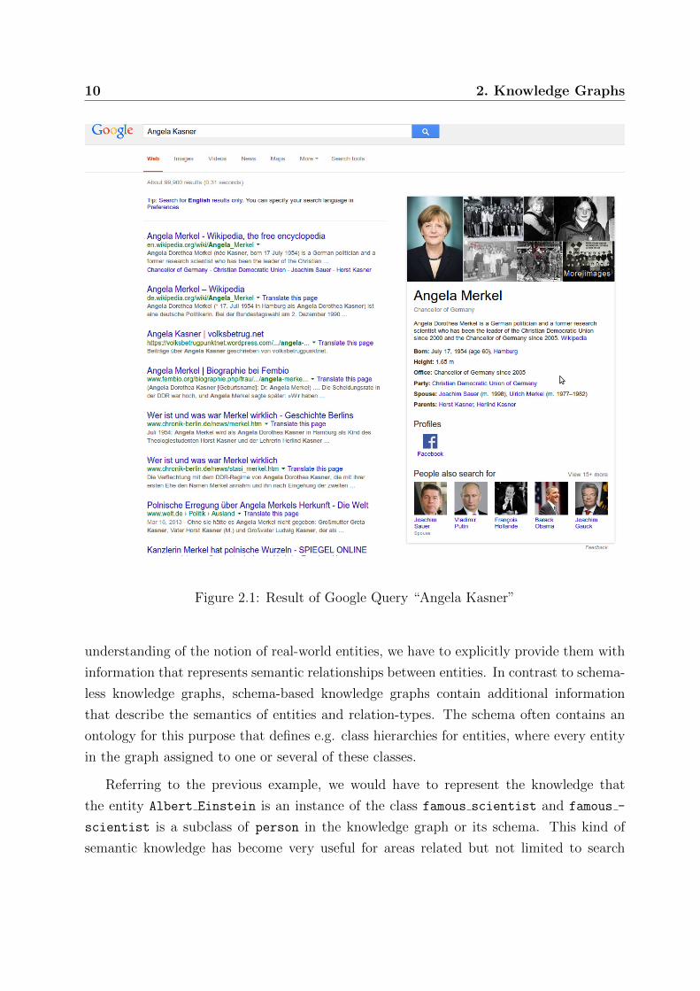
Figure 2.2: Mobile smart assistants answering the question about the height of the EiffelTower. Image was taken from [109]
and question answering, as successfully demonstrated by Google’s search engine or IBM’s
Watson system. As an example, consider the question “who is the most famous scientist?”.
If we assume that a machine can understand that this question is about a person (e.g.
through the keyword “who”), the search space can already be restricted to person entities
represented in the knowledge graph.
Further, the knowledge graph can be exploited to aggregate more information than
given by a query to guess on the intentions of the users. Assuming that the search query
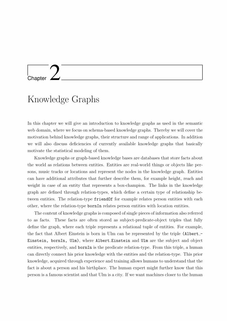
“Angela Kasner” is entered in a search application (e.g Google), the search engine will
recognize that the query is about Angela Merkel, the current chancellor of Germany, since
it automatically exploited information from the knowledge graph (Figure 2.1).1 As a con-
sequence, the combination of Angela Kasner and Angela Merkel results in highest ranked
documents that are discussing the past of Angela Merkel. This can be interpreted as
the attempt of the machine to guess on the intention of the user, which in this case was
interpreted as the interest in getting biographic information on Angela Merkel.
In the domain of natural language processing, the information provided by knowledge
graphs is exploited for word-sense disambiguation, entity resolution and relation extraction.
1The Google Knowledge Graph is in part powered by Freebase [8] which e.g. links “Angela Kasner”and “Angela Merkel” to the same Freebase id m/0jl0g by the relation-type alias (which is also the basisfor the “Also known as” listing in Freebase entries).
12 2. Knowledge Graphs
Table 2.1: Abbreviations for URIs used in this work for better readability of triples.
Name-Space Abbreviationhttp://dbpedia.org/ontology/ dbpo:
http://dbpedia.org/resource/ dbpr:
http://www.w3.org/1999/02/22-rdf-syntax-ns# rdf:
http://www.w3.org/2000/01/rdf-schema# rdfs:
The combination of natural text extraction methods and knowledge graphs have led to very
sophisticated question answering system, as impressively shown by the IBM Watson system
which beat human champions in Jeopardy!, but also by popular smart mobile assistants
e.g. Apple’s Siri, Microsoft’s Cortana or Google Now (Figure 2.2).
Today, a wide range of knowledge-graphs are available, in part domain specific as e.g.
the Gene Ontology [2], but also general purpose ones like e.g. Freebase [8] or YAGO [46]
that contain general knowledge partially extracted from Wikipedia, the currently biggest
online encyclopedia. Freebase has been acquired by Google in 2010 and powers in part the
Google Knowledge Graph [98] and the recently published Google Knowledge Vault [25].
This graph supports Google’s search engine and is also exploited in various other applica-
tions developed by Google as for example Top Charts or Google Now. In addition, thanks
to the effort of the linked open data initiative [6], many of these knowledge graphs have
been interlinked, allowing a facilitated integration of various data sets in an application.
2.1 Knowledge-Graphs are RDF-Triplestores
Generally, graph based knowledge-bases like YAGO [46] or DBpedia [66] store their facts
as triples that more or less follow the W3C Resource Description Framework (RDF) [61]
standard. The RDF defines the data model for the Semantic Web. The choice to represent a
labeled, directed graph through triples was driven by the goal of least possible commitment
to a particular data schema, by using the simplest possible structure for representing such
information. RDF allows a rich structuring of semantic web data. In this section, we will
only cover the most important concepts relevant for this thesis and refer the interested
reader to [44]. Further we will use the name-space abbreviations shown in Table 2.1 for
better readability of triples.
2.1 Knowledge-Graphs are RDF-Triplestores 13
2.1.1 RDF-Triple Structure
RDF-triples follow a subject-predicate-object (s, p, o) pattern, where the subject is filled
through resources or blank nodes, the predicate resource represents the relationship2 be-
tween the subject and the object entity and the object can be resources, blank nodes or
literals.
Resources
In a RDF-triple, resources are represented by their Internationalized Resource Identifier
(IRI), a generalization of the Uniform Resource Identifier (URI), which can be an Uniform
Resource Locator (URL). Resources are the “things” in the knowledge graph like persons
or locations but also abstract concepts. Throughout the rest of this thesis, we generally
refer to resources that occur as subject or object in a RDF-triple if we speak of entities.
Additionally, the term relation-type always refers to resources that occur as predicates in
such a triple. As an example, consider the triple (dbpr:Angela Merkel, dbpo:birthPlace,
dbpr:Hamburg), extracted from DBpedia. In this triple, dbpr:Angela Merkel is the sub-
ject entity, dbpr:Hamburg the object entity and dbpo:birthPlace the predicate relation-
type that relates Angela Merkel to her birthplace Hamburg.
Literals
Literals are the direct embedding of values into the graph such as dates, strings or numbers
that describe a resource. The different textual representations for the entity that represents
the resource Angela Merkel, “Angela Merkel” and “Angela Kasner” or the birth-date are
for example literals. In difference to resources or blank nodes, literals should never occur
as subjects in a triple, or in other words, literal nodes in the graph are not supposed to
have any outgoing links.
Blank Nodes
Blank nodes are auxiliary nodes that do not provide any explicit content but allow the
construction of e.g. higher order facts. In order to differentiate resources from blank nodes,
each blank node is identified by a node identifier instead of an IRI. The node identifier is
required to enable multiple resources to reference on the same blank node. Blank nodes
2Also often referred to as properties or relation-types.
14 2. Knowledge Graphs
are omitted from upcoming discussions, because they are not explicitly considered by the
methods proposed and discussed in this work for knowledge graph modeling.
2.1.2 Schema Concepts
As mentioned in the introduction of this chapter, entities are generally typed in schema-
based knowledge graphs, meaning that they have been assigned to predefined classes that
are organized in an ontology that is part of the schema. An ontology describes a data model
of the target domain of the graph including the vocabulary that describes this domain. In
addition, these ontologies can be used to represent implicit knowledge by defining subclass
hierarchies which can be materialized through reasoning. For example, consider all triples
of the form (<?>, rdf:type, dbpo:MusicalArtist) present in DBpedia, where <?> is used
as a variable for all entities that have been assigned to the class MusicalArtist. With an
ontology that contains the subclass relationship (dbpo:MusicalArtist, rdfs:subClassOf,
dbpo:Person), we can implicitly represent the knowledge that all entities that are musical
artists are also persons.
Light-weight ontologies can be defined through the RDF-Schema (RDFS) [20] concepts,
which allow the definition of classes and class hierarchies. In Table 2.3 a small section of
the DBpedia ontology is represented in RDFS, the corresponding ontology is visualized
below in Figure 2.3. More complex ontologies can be constructed with the Web Ontology
Language (OWL) [85] but in general, more complex ontologies increase the computational
costs for reasoning. When constructing ontologies, there is always a trade-off between the
complexity of the defined ontology and the efficiency of the appropriate reasoner. We refer
to [1] for more details on OWL.
Besides the entities that can be semantically refined through ontologies, also relation-
types can be semantically described using RDFS as well. In knowledge graphs, generally
two types of relation-types exist, DatatypeProperties and ObjectProperties, where the for-
mer relates entities to literals and the latter relates entities to entities. Also, relation-
types can form hierarchies. In correspondence to rdfs:subClassOf, RDFS offers the
rdfs:subPropertyOf concept to define hierarchies of relation-types that can be exploited
by reasoners. A comprehensible example for such a hierarchy are couples that have a mar-
riage and those that have a happy marriage. Clearly, the person entities that are related
by a happy marriage are also implicitly related by marriage.
Besides enabling the definition of relation-type hierarchies, RDFS offers the concepts
rdfs:domain and rdfs:range to implement type-constraints. These two concepts describe
2.1 Knowledge-Graphs are RDF-Triplestores 15
Table 2.2: Defining type-constraints on the relation-type dbpr:bandMember using RDFS
id Subject Predicate Object1 dbpr:bandMember rdfs:domain dbpo:Band
2 dbpr:bandMember rdfs:range dbpo:Person
Table 2.3: Section extracted from the DBpedia ontology represented in RDFS. Breakdownof abbreviations can be inferred from Table 2.1
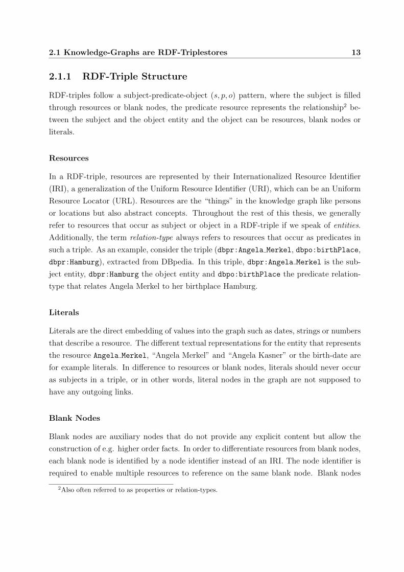
Subject Predicate Objectdbpo:Artist rdfs:subClassOf dbpo:Person
dbpo:MusicalArtist Gibbons rdfs:subClassOf dbpo:Artist
dbpo:Writer rdfs:subClassOf dbpo:Artist
dbpo:Singer rdfs:subClassOf dbpo:MusicalArtist
dbpo:MusicalDirector rdfs:subClassOf dbpo:MusicalArtist
dbpo:MusicComposer Gibbons rdfs:subClassOf dbpo:Writer
dbpo:SongWriter rdfs:subClassOf dbpo:Writer
the semantics of a relation-type by explicitly defining which entity classes should be related.
Obviously, the relation-type dbpo:birthPlace should not be used to relate instances of the
class dbpo:Person with each other, but persons to locations (dbpo:Location). In Table
2.2 type-constraints on the relation-type dbpr:bandMember are shown. dbpr:bandMember
is defined to relate instances of the class dbpo:Band to instances of the class dbpo:Person.
Person
Artist
Writer MusicalArtist
SongWriter MusicComposer MusicalDirector Singer
subClassOf
subClassOf subClassOf
subClassOf subClassOf subClassOf subClassOf
Figure 2.3: Illustration of ontology described in Table 2.3
16 2. Knowledge Graphs
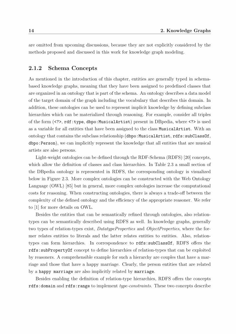
Table 2.4: Example facts from DBpedia regarding the resources Billy Gibbons and Nick-elback. The breakdown of abbreviations can be inferred from Table 2.1
id Subject Predicate Object1 dbpr:Billy Gibbons dbpo:associatedBand dbpr:Nickelback
2 dbpr:Billy Gibbons rdf:type dbpo:Person
3 dbpr:Nickelback rdf:type dbpo:Band
4 dbpr:Billy Gibbons dbpo:instrument dbpr:Fender Telecaster
5 dbpr:ZZ Top dbpo:bandMember dbpr:Billy Gibbons
6 dbpr:Billy Gibbons dbpo:genre dbpr:Hard rock
7 dbpr:Nickelback dbpo:genre dbpr:Hard rock
BillyGibbons
FenderTelecaster
ZZ TOP
Person
HardRock
Nickelback
Band
instrument
bandMember
type
genre
associatedBand
type
genre
Figure 2.4: Graph representation of facts from Table 2.4
2.1.3 Knowledge Retrieval in Knowledge Graphs
As previously shown, RDF provides an easy and comprehensible way to describe and define
knowledge as a graph of facts. In the following, we will show in a more concrete case how
actual knowledge (and its facts) are represented and made accessible to machines.
In Table 2.4, a RDF-Triplestore consisting of 7 triples extracted from DBpedia is shown.
From the first triple (dbpr:Billy Gibbons, dbpo:associatedBand, dbpr:Nickelback), a
human can easily understand that it describes a person named Billy Gibbons, that is
somehow associated with the rock band Nickelback.3 A human with more expertise on
the band ZZ-Top could automatically connect other knowledge about Billy Gibbons as
3Billy Gibbons appeared on Nickelback’s album All the Right Reasons.
2.2 Knowledge Graph Construction 17
e.g. that he is a guitarist of the rock band ZZ-Top. A similar principle is applied in
knowledge graphs where the connections to associated information of entities are the links
in the graph. Based on all facts of Table 2.4, we are able to construct a small knowledge
graph (Figure 2.1.3) that can be traversed by machines, or queried, to aggregate relevant
information.
RDF-structured data sets can be queried to retrieve and manipulate data. One of
the most popular query languages for this task is the semantic query language SPARQL4,
which shares common principles with many other query languages such as SQL. This query
language allows a user to define queries that consist of triple patterns with disjunctions
and conjunctions of these patterns. The following simple example shows how SPARQL
works in principle:
PREFIX dbpr: <http://dbpedia.org/resource/>
PREFIX dbpo: <http://dbpedia.org/ontology/>
PREFIX rdf: <http://www.w3.org/1999/02/22-rdf-syntax-ns#>
SELECT ?somebody
WHERE{
?somebody dbpo:instrument dbpr:Fender_Telecaster.
?somebody rdf:type dbpo:MusicalArtist.
dbpr:ZZ_Top dbpo:bandMember ?somebody.
}
In the top part we simply defined abbreviations for the name-spaces for better readability
of the subsequent SPARQL query (PREFIX). In the actual SPARQL query, we ask for
an entity in the database (denoted by ?somebody) that is a musical artist (?somebody
rdf:type dbpo:MusicalArtist) and band member of the rock band ZZ-TOP that plays
a Fender Telecaster. When using the SPARQL-Endpoint5 of DBpedia to evaluate the
above query 6, the entity dbpr:Billy Gibbons is returned.
2.2 Knowledge Graph Construction
In this section, we will describe how knowledge graphs are constructed in principle. Basi-
cally, knowledge graph construction can be achieved by different kinds of approaches that
4SPARQL Protocol and RDF Query Language.5Services that process SPARQL queries.6http://dbpedia.org/sparql
18 2. Knowledge Graphs
require different levels of human involvement. The order in which these approaches are
described next approximately reflects the size of the resulting knowledge graph and the
chronology in which they have been applied.
2.2.1 Curated Approaches
Curated approaches contain the earliest knowledge graphs that were mainly constructed by
a small group of human experts. The first knowledge graphs for computers, originally de-
noted as semantic nets, were invented in 1956 for machine translation of natural languages
[93]. A prominent example for a widely used knowledge graph, initially constructed by
the Cognitive Science Laboratory of Princeton University, is WordNet [33]. WordNet has
a central role in many applications in the natural language processing domain. From all
available knowledge graphs, curated knowledge graphs are clearly the most accurate ones
and complete ones. Unfortunately, due to their dependence on human experts, they are
not very scalable and normally cover highly specialized domains that can be represented
by small graphs.
2.2.2 Collaborative Approaches
Collaborative knowledge graph construction relies on a large community of voluntary con-
tributors that add new facts to the knowledge graph. Additionally, the editing and quality
control is also based on these contributors. Even though collaborative approaches can
lead to large knowledge bases, such as Wikipedia [37] or in part the Freebase [8] knowl-
edge graph, their scalability is always dependent on their popularity; popularity has direct
impact on the size of the community of contributors. In addition, the growth of such knowl-
edge graphs will eventually decrease, because it becomes harder for the broad community
of contributors to add new triples to the graph. Besides the graph in a whole, also the
contained topics are dependent on popularity and as a consequence, less popular content
generally lacks extensive revision.
2.2.3 Automated Approaches on Semi-Structured Textual Data
Fully automatic construction approaches such as YAGO [46], DBpedia [66] or Freebase [8]
extract their content from semi-structured sources such as tables (e.g. Wikipedia Infoboxes)
and the schema (e.g. WordNet Taxonomy or the Wikipedia category system) or structured
sources such as other knowledge graphs. The concepts extracted from semi-structured data
2.2 Knowledge Graph Construction 19
often lack proper disambiguation. For example, in Wikipedia Infoboxes a person can be
related by multiple concepts to his birthplace, such as “Place of birth”, “born in” or
“birthplace”, which all have the same semantics. Similarly, different ontologies used by
different knowledge graphs are often not properly interlinked. These ontologies often share
semantically equal entities and classes, but the mapping of entities and classes between
the ontologies is often absent. To solve these issues, the extraction of facts is backed
by hand-curated rules that properly resolve disambiguation. The advantage of this kind
of automated approach is its scalability and the reduced amount of human involvement,
leading to very accurate knowledge representations. The growth and quality of knowledge
graphs that are constructed this way are not directly dependent on a large community
of voluntary contributors, but on the quality of their data sources. These sources are of
course dependent on a large community of contributors that provide the semi-structured
data. As a consequence, these automatically constructed knowledge graphs also suffer from
similar deficiencies as the collaborative constructed ones, especially incompleteness.[102]
2.2.4 Automated Approaches on Unstructured Textual Data
Due to the problems observed in the other three approaches, the main goal of the most
recent research efforts is the construction or completion of knowledge graphs based on
unstructured textual data. In Wikipedia, the currently largest online encyclopedia on the
web, only a small fraction of its content is covered by the semi-structured infoboxes. The
majority of information in Wikipedia, and generally on the Web, is contained in unstruc-
tured textual data, that is the natural language description of the articles. The NELL
(Never Ending Language Learner) project [16] tries to “read the web” to extract new facts
from unstructured textual web content. Recently, [25] proposed an approach where the
statistical modeling of existing knowledge graphs (Freebase) can be combined with rela-
tion extractors applied on unstructured text documents to complement the content of these
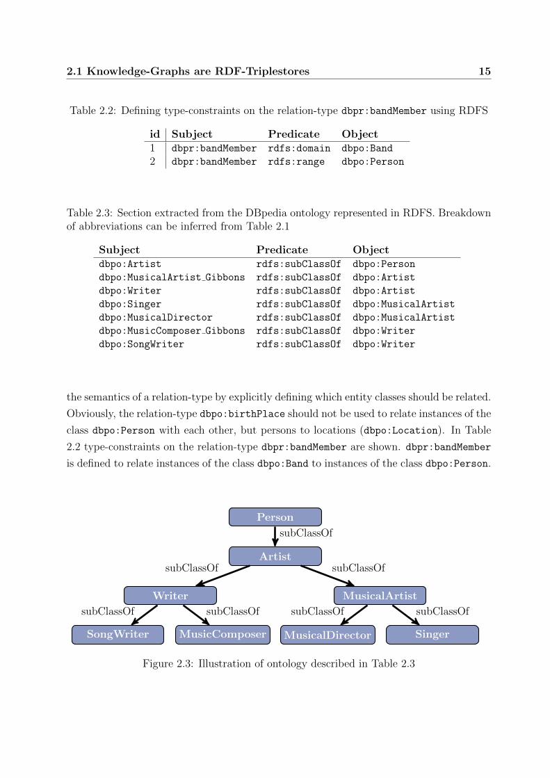
knowledge graphs accurately on a large scale. The principle of this approach is illustrated
in Figure (2.5). In the first step, a text extraction tool is applied on textual data for
triple extraction, which additionally provides a measure of confidence (a probability) that
represents the belief of the extractor that this relation is true. In parallel, the confidence of
statistical models which have been applied to the knowledge graph data is retrieved for the
same triple. These statistical models can be latent variable models, which are in the focus
of this thesis, but also graph feature models (e.g. path ranking algorithm) are exploited
for this task ([25] used a combination of both). For the final decision on which triples are
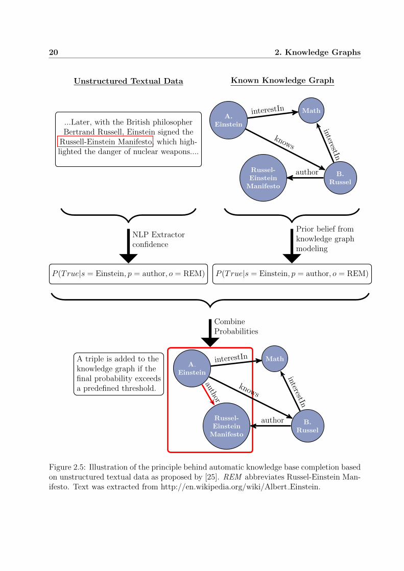
20 2. Knowledge Graphs
Unstructured Textual Data
Russel-Einstein-Manifesto
...Later, with the British philosopherBertrand Russell, Einstein signed the
Russell-Einstein Manifesto, which high-lighted the danger of nuclear weapons....
Known Knowledge Graph
A.Einstein
B.Russel
Math
Russel-EinsteinManifesto
knows
interestIn
interestIn
author
P (True|s = Einstein, p = author, o = REM) P (True|s = Einstein, p = author, o = REM)
NLP Extractorconfidence
Prior belief fromknowledge graphmodeling
A.Einstein
B.Russel
Math
Russel-EinsteinManifesto
CombineProbabilities
A triple is added to theknowledge graph if thefinal probability exceedsa predefined threshold. knows
interestIn
interestIn
author
author
Figure 2.5: Illustration of the principle behind automatic knowledge base completion basedon unstructured textual data as proposed by [25]. REM abbreviates Russel-Einstein Man-ifesto. Text was extracted from http://en.wikipedia.org/wiki/Albert Einstein.
2.3 Popular Knowledge Graphs 21
added to the graph, the confidences provided by the various methods are combined. It was
shown in [25] that this approach significantly increased the accuracy of relation extraction
from natural language text.
2.3 Popular Knowledge Graphs
In this part we will describe three widely used knowledge graphs in more detail that were
also the primary source of data of the experiments conducted in this thesis, namely DBpedia
[66], Freebase [8] and YAGO [46]. All of these knowledge graphs heavily rely on data from
Wikipedia and are part of the Linked Open Data (LOD) cloud, an initiative that aims for
the goal of interlink various open RDF-structured data sets on the web [6]. The Wikipedia
online encyclopedia is with no doubt one of the most widely used source of knowledge in
the Internet today. Its content is maintained by thousands of contributors and used by
millions of people daily. Even though Wikipedia contains a lot of information, its search
and querying capabilities are limited to find whole articles. For example, it is difficult to
find all mountains above a certain height in the German alps. As already discussed in this
chapter, these kind of queries can be easily answered by knowledge graphs, because they
contain structured content.
2.3.1 DBpedia
The DBpedia [66] community project was started in 2006 with the goal to create a struc-
tured representation of Wikipedia that follows the Semantic-Web standards. DBpedia
serves as a machine accessible knowledge graph that enables complex querying on data from
Wikipedia. Besides the natural language content, Wikipedia articles are often enriched in
structured information such as Infobox templates, article categorizations, geo-coordinates
and links to other online-resources. Hereby, Wikipedia Infoboxes are the most valuable
source of information for DBpedia, because their purpose is to list the most relevant facts
of the corresponding article (especially for famous people or organizations). DBpedia pro-
vides an automatic extraction framework to retrieve facts from Wikipedia articles and
stores them in a RDF-Triplestore. Here, the heterogeneity in the Wikipedia Infobox sys-
tem has been a problem, because the authors did not follow one standard structure, but
used different Infoboxes for the same type of entity or different relation-type names for
semantically equal relationships.
A big step forward in terms of data quality could be achieved in 2010, when a community
22 2. Knowledge Graphs
effort has been initiated to homogenize and disambiguate the description of information in
DBpedia. Through this effort, an ontology schema has been developed and the alignment
between Wikipedia Infoboxes and this ontology has been leveraged by community-provided
mappings that disambiguate relation-types, entities and classes. Besides disambiguation,
these mappings also include the typing of resources and specific data-types for literals. In
absence of those mappings, the resources extracted from the Infoboxes are saved as literal
values, because their semantics are unclear to the extractor. However, even though data
quality is improving, it is unlikely that DBpedia will reach the quality of manually curated
data sets. In the current release (DBpedia2014), the DBpedia ontology consists of 658
classes which are related by 2,795 different relation-types. These 658 classes count 4,233,000
instances, of which 735,000 are places, 1,450,000 persons and 241,000 organizations. In
total, the English version of DBpedia contains 583 million facts, but multilingual DBpedia
(129 languages are included) counts approximately 3 billion RDF-triples. In addition,
DBpedia provides a large amount of links to external data sets on instance and schema
level.
DBpedia has become a central hub of the Linked Open Data cloud and numerous
applications, algorithms and tools are using its content. In addition, DBpedia provides
different types of data sets for various purposes. One example is the Lexicalization data
set which is especially useful in NLP related tasks. This data set contains alternative
names for entities and properties together with several measures that indicate observed
frequency of the ambiguity of terms.
2.3.2 Freebase
Similar to DBpedia, Freebase [8] is also a RDF-based graph database, but in contrast to
DBpedia, Freebase does not solely rely on structured information extracted from Wikipedia
Infoboxes. Freebase also integrates information from many other external databases, for
example MusicBrainz, WordNet and many more. In addition, facts are directly added
and reviewed by a large community of voluntary contributors. This is a big difference to
DBpdia, where data could only be changed by editing the corresponding Wikipedia article.
In Freebase, real world things or concepts are termed as topics, where each topic has an
article on Freebase. Not all entities in Freebase are topics, there also exist literals that relate
specific values to the topics. In addition, blank nodes are used to represent more complex
facts. Similar to DBpedia, Freebase also contains ObjectProperties and DatatypeProperties.
The former relation-types relate topics to entities that are no literals and the latter relate
2.3 Popular Knowledge Graphs 23
topics to (typed) literals. In Freebase, relation-types have type-constraints, which are
denoted as expected types that correspond to the rdfs:range and rdfs:domain constraints.
The Freebase ontology (called Schema) does not represent an inheritance hierarchy, but
groups entity types into domains, which can also be edited by the community using an
online interface.
Currently, Freebase consists of 47 million topics, 70,000 relation-types and 2.7 billion
facts about them. In 2010, Freebase (Metaweb) was acquired by Google and now powers in
part Google’s Knowledge Graph [98] and the recently published Google Knowledge Vault
[25]. In 2014, Google announced a retirement of Freebase in mid 2015 and that it will be
integrated in Wikimedia-Foundation’s Wikidata project [110].
2.3.3 YAGO
YAGO (Yet Another Great Ontology) is an automatically generated high quality knowledge
graph that combines the information richness of Wikipedia Infoboxes and Wikipedia’s
category system with the clean taxonomy of WordNet. The YAGO project is basically
motivated by two observations: First, Wikipedia offers a very broad view on the knowledge
of the world, but its category system is not well suited as an ontology. Second, WordNet
offers a very clean and natural ontology of concepts, but falls short in describing real
world entities like authors, musicians etc. YAGO maps the Wikipedia categories on the
WordNet ontology with a precision of 95%, thereby successfully linking these two sources of
information. The YAGO entities are assigned to more than 350,000 different classes and all
relations in YAGO are attached with a confidence value. It further defines a simple model,
the YAGO model, that extends RDFS to allow the representation of n-ary relations, but
which in contrast to complexer ontology languages, such as OWL-Full, is still decidable.
The n-ary relations are realized by introducing fact identifiers that can easily be integrated
in RDF. These identifiers represent blank nodes in the graph that refer to whole facts,
which in turn can be used as reference in other facts to realize n-ary relations. As an
example, the fact
Albert Einstein hasWonPrize Nobel Prize in Physics inYear 1921
can be represented by determining the core fact and assigning an identifier to it
#1: Albert Einstein hasWonPize Nobel Prize in Physics
and using this identifier as reference for the second fact
#2: #1 inYear 1921
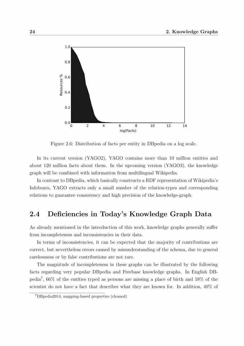
24 2. Knowledge Graphs
0 2 4 6 8 10 12 14
log(Facts)
0.0
0.2
0.4
0.6
0.8
1.0
Reso
urces %
Figure 2.6: Distribution of facts per entity in DBpedia on a log scale.
In its current version (YAGO2), YAGO contains more than 10 million entities and
about 120 million facts about them. In the upcoming version (YAGO3), the knowledge
graph will be combined with information from multilingual Wikipedia.
In contrast to DBpedia, which basically constructs a RDF representation of Wikipedia’s
Infoboxes, YAGO extracts only a small number of the relation-types and corresponding
relations to guarantee consistency and high precision of the knowledge-graph.
2.4 Deficiencies in Today’s Knowledge Graph Data
As already mentioned in the introduction of this work, knowledge graphs generally suffer
from incompleteness and inconsistencies in their data.
In terms of inconsistencies, it can be expected that the majority of contributions are
correct, but nevertheless errors caused by misunderstanding of the schema, due to general
carelessness or by false contributions are not rare.
The magnitude of incompleteness in these graphs can be illustrated by the following
facts regarding very popular DBpedia and Freebase knowledge graphs. In English DB-
pedia7, 66% of the entities typed as persons are missing a place of birth and 58% of the
scientist do not have a fact that describes what they are known for. In addition, 40% of
7DBpedia2014, mapping-based properties (cleaned)

2.4 Deficiencies in Today’s Knowledge Graph Data 25
all countries miss a capital and 80% of the capitals do not have a leader. Even 2% of the
entities are not assigned to any class. In Freebase, 71% of persons are missing a place
of birth and 75% do not have a nationality [25]. Generally, it can be expected that the
amount of missing information is even higher for less popular entities and relation-types.
Besides missing information, the amount of triples for each entity also varies to a large
extent in the knowledge graphs, as shown in Figure 2.6 for DBpedia. It can be observed
that the distribution is heavy-tailed (note the log scale) and only a minority of about
16,000 out of 4.5 million entities in DBpdia takes part in more than 100 facts (triples).
However, this small fraction of entities (0.34%) occurs in 18.7% of all facts. About 50% of
all entities occur in less than or equal to 5 facts and 500,000 (11%) have only one fact. It
can be concluded that the vast majority of entities in DBpedia is not well described, while
in contrast a large amount of information is available for a very small fraction of entities.
The reasons for this incompleteness are manifold, but the major cause lies in the fact
that most of the information available today is contained in natural text documents which
is hard to extract. It is certain that it is intractable for the community of voluntary
contributors to structure this data manually, even a reliable quality control for all facts
stored in knowledge graphs has become unreachable.
Today, growth and quality of knowledge graphs is still highly dependent on the various
communities of voluntary contributors. Recently, it has been observed that the growth
of Wikipedia, which serves as a central knowledge repository for many knowledge graphs,
has eventually plateaued [101]. There are multiple explanations for this observation, for
instance that due to the size of the database and the large community of contributors the
internal bureaucracy has increased. Nevertheless, one of the main reasons lies in the fact
that the amount of opportunities to contribute knowledge for the broad majority of the
community decreases with the size of the database. This fact also reflects the observation
that in Wikipedia a decline in editor and page growth was observed [101].
To tackle the deficiencies observed in available knowledge graphs, automatic approaches
that support quality control in knowledge graphs, and boost the growth and increase
completeness are in great need. In Section 2.2.4, approaches are described that tackle the
relation mining from unstructured textual data sources by exploiting statistical models
for knowledge graphs. These models are capable of evaluating triple quality in knowledge
graphs, which can be exploited for completion and cleansing tasks for such graphs. Latent
variable models have been successfully exploited for the statistical modeling of knowledge
graphs and it was shown that these models scale to web-scale data sets.

26 2. Knowledge Graphs
Chapter 3Representation Learning in Knowledge
Graphs
In this chapter, we will cover the basics of representation learning in knowledge graphs.
First, we will give a brief introduction to representation and relational learning, before we
will discuss three representation learning algorithms in more detail that have been applied
to knowledge graph data, namely RESCAL [82], Translational Embeddings [9] and the
neural network approach used in the recent Google Knowledge Vault project [25].
3.1 Representation Learning
Generally, the predictive modeling capabilities of machine learning algorithms rely on the
quality of the data that define the problem context. Here, quality refers to different impor-
tant aspects that can be considered in different ways by these models: First, the noise in
the data. Machine learning algorithms are data driven models, therefore it is not surprising
that it is harder for them to detect dependencies and patterns in noisy data since noise can
distort and mask important signals and correlations. Noise in the data is present in every
real-world data set such as e.g. data recorded by sensor measurements of machines used in
an industrial production environment. Reasons for noise in the data can be manifold and
its removal is often connected to a trade-off between noise reduction and signal loss. In
machine learning, robust and generalizing models on noisy data can be trained by applying
regularization on the model parameters during training.
Second, the capability of the features present in the data to sufficiently explain the
distribution of the target variables of the problem task to solve. Obviously, to recognize
28 3. Representation Learning in Knowledge Graphs
if the recorded data contains enough information to model a problem task can be very
challenging. There might be confounding factors that are not recorded in the data, but
have a dramatic impact on the target outcome. Dependent on the importance of the
confounding factors for the modeling, a learning task can become infeasible. In a less
dramatic case, but still very challenging, the recorded factors (features) contain enough
information to reason on the target distribution, but correlations are hidden or not obvious
enough to be easily recognized by the learning algorithm. As a simple example, consider a
lung cancer risk prediction task where no information about the patient’s smoking habits
are included in the data (e.g. if the patient is a smoker and how many cigarettes are
consumed every day). It is generally known that there is a strong correlation between
smoking and lung cancer risk. However, in the latter case there might be other features
present in the data from which we could conclude on the smoking habits of a patient
(e.g. a combination of age, teeth color, blood pressure, blood sodium level etc.), which
themselves do not have an obvious correlation with lung cancer. Traditional machine
learning methods have problems to extract and organize such discriminative information
from the data. In this situation, feature engineering can often be applied to manually
or semi-automatically construct additional features that incorporate human prior (expert)
knowledge which explain the target variables more obvious to the learning algorithm. For
the previous example we would introduce a “smoker” feature in the data that is derived
from the other features by a human expert or through some given formula exploited as
basis function. Unfortunately, feature engineering has the disadvantages that it can be
quite labor-intensive and often domain experts have to be consulted for suitable feature
construction (e.g. in the lung cancer risk prediction example we would need physicians
that are familiar with clinical traits of smokers).
Representation Learning, often also referred to as feature learning, proposes a different
approach that avoids the dependence on labor extensive feature engineering, but tries to
automatically discover good latent features that disentangle hidden correlation present in
the data. However, in difference to the raw input or hand engineered features which most
often have a clear interpretation, these learned latent features are often hard to interpret.
In Representation Learning a transformation of the raw input data into a new latent
feature space is learned, where this feature space consists of explanatory factors that are
more useful for a classifier or other predictor. Even though this latent feature space is a
better basis for the learning task to solve than the feature space spanned by the original
raw features, this does not mean that it has to be more complex. In fact, the opposite is
3.1 Representation Learning 29
often the case since raw data often contains redundant dependencies or large amounts of
other dispensable information that is not necessary for representing the underlying data
generating function. Tensor/matrix factorization or Autoencoders are typical approaches
where the latent feature space is enforced to be much smaller than the original feature space
in order to learn the most general factors that are important to explain the distribution of
the data. [45, 41, 105, 51]
Expressive new representation of input data can be learned in a supervised or unsu-
pervised setting. In the supervised setting, the new representations are directly learned
with respect to the given labels from the supervised task, thereby leading to latent factors
that disentangle correlations to the target variable. This approach is often executed with
neural networks, where the first layer is responsible for learning the first raw feature trans-
formation which is combined to generate the final output, or in case of deep networks (e.g.
convolutional neural networks for image recognition), to form the input for further feature
transformations to realize complex latent representation hierarchies.
Learning good representations for a target task can be difficult if the amount of labeled
training data falls short in comparison to the complexity of the learning problem. Good
representations can also be learned in an unsupervised settings and exploited, if desired,
in a supervised learning task as a fixed input data transformation or as initialization
for the representation layer in a neural network. It is often convenient to assume that
representations that explain much of the distribution of the input data tend to also explain
much of the target distribution. In addition, generally plenty of data for a unsupervised
learning scenario is available or can be collected very easily. As an example, consider a
document topic classificator which exploits latent representations of words. Intuitively, we
would directly assume that the topic of a document is dependent on the distribution of
words in a document and therefore learning representations that explain the distribution
of words in a document, independent from the topic, should be beneficial for the topic
classification. In difference to the topic learning task, where only a limited amount of
labeled training data is available, for the unsupervised learning task that tries to learn
good representations of words that explain the distribution of words in documents, almost
unlimited amounts of training data is available.[28, 86]
Probably the best known representation learning approach is the Singular Value De-
composition (SVD), which is also exploited in the Principal Component Analysis (PCA)
and learns latent factors that explain most of the variance observed in the data. Non-
negative matrix factorization has been exploited in text or image processing [59, 63] where
30 3. Representation Learning in Knowledge Graphs
in case of the images, the latent factors could be interpreted as local structures like eyes,
ears or noses. Factorization Machines [89] have been quite successful in recommendation
settings, learning latent representations for users and items. Higher order tensor factor-
ization methods were used on various data set such as EEG data where the latent factors
have been exploited to analyze epileptic seizures [76]. Tensor factorization has also been
exploited in image processing tasks e.g. for Tensor Faces [107], a generalization of Eigen-
faces [106], that additionally considers various perspectives of face images as additional
modes in the tensor.
More recently, deep learning approaches have gained much popularity and have been
applied in a variety of fields, including speech recognition and signal processing, object
recognition, natural language processing (NLP) and multi-task learning, often representing
the current state of the art with leading performance on various benchmark sets [22, 53,
72]. The representations learned by these models, as for example in convolutional neural
networks in the context of images, have even outperformed approaches that exploited
sophisticated feature engineering through human experts. We refer to [4] for a very good
review on representation learning with deep architectures at this point.
In difference to the various types of data representation learning has been applied to,
with knowledge graphs we are dealing with graph structured data where the nodes are de-
fined through their connections in the graph and not solely on a fixed set of features that
describe them. Similar to the word setting in NLP, the raw data is often purely symbolic,
meaning that we have just the URI of the entity (or words in the NLP setting) and the
context this symbol appears in without any features that describe the characteristics of
the entity. Having expressive distributed representations of entities that contain the gen-
eral explanatory factors for the dependencies observed in the graph makes these symbolic
URIs comparable, meaning that similar entities that share a similar representation should
have similar connections in the graph. In a sense, the goal of representation learning in
knowledge graphs is to disentangle the semantics of entities solely based on the observed
relationships between entities in the graph. Learning from these relationships is referred
to as Relational Learning which we will discuss in the next section.
3.2 Relational Learning
In (traditional) non-relational learning settings, the data consist mainly of features that
describe measured characteristics of instances (or entities), as for example in an arbitrary
3.2 Relational Learning 31
population study that collects attributes like size, age, gender, employee, academic degree
etc. of different persons. Generally when dealing with this kind of data sets, independence
between these instances is assumed to simplify the learning problem. As a consequence,
the learning algorithm will only model dependencies between the given features and some
target variable we want to predict. For example, consider the learning problem where we
want to predict the income of persons based on the schematically described data set from
the previously mentioned population study. In this case, the learner will predict the income
for each person individually without considering any dependence on the other persons in
the data set.
In a relational learning setting we eventually discard this strict independence assump-
tion by exploiting data that explicitly reflects dependencies between the instances in the
learning algorithms. Referring to the previous example, we might also know which of the
persons in the data are friends or work in the same company. Assuming dependencies
between entities in the data generally increases the complexity of the learning problem,
which can become intractable. Today’s relational learning algorithms have managed to
decrease complexity to a manageable size allowing an application on even very large data
sets.
There are dependency patterns that are present in relational data that can be exploited
by relational learning algorithms, but not by non-relational learners [78]. In relational data,
it is often observed that entities with similar characteristics are related to each other. This
observation is termed homophily and is exploited for predicting relations between similar
entities, but also to predict attributes. As an example, persons with the same age, income
and academic background might be employed at the same company. Further, if they work
in the same company, they might even know each other or are even friends. Stochastic
equivalence on the other hand describes the observation that similar entities form groups
and that the relationships observed in the graph can be explained by the relationships
of these groups. This dependency can be exploited for clustering of entities, but also
for predicting new relationships, since the members of one group tend to have similar
relationships to members of other groups. Additionally, the relational data might contain
global dependencies, which can be understood as (complex) rules that can be exploited by
the learning algorithm. For example, actors that played in movies with high ratings are
probably rich.
The exploitation of these dependencies, which are also present in graph based knowledge
representations, make relational learning algorithms especially attractive for applications
32 3. Representation Learning in Knowledge Graphs
in knowledge graphs. There exist a wide range of relational learning algorithms and in
this work we only consider statistical relational learning methods, which model statistical
dependencies observed in the knowledge graph. More specific, we focus on latent variable
methods that learn distributed representations for entities and relation-types and have
been successfully applied to the relational domain. The main application of these methods
in knowledge graphs is link-prediction, meaning that the learning algorithms propose new
relations between existing entities that can be added to the graph to enrich its knowledge
content. Link-prediction is the basis for tasks related to knowledge graph cleansing and
completion and plays a central role in automatic knowledge graph construction methods
based on unstructured textual information (see Chapter 2.2.4). Further, the learned dis-
tributed representations of entities can be exploited for link-based clustering, but also for
entity resolution, often used in tasks related to the disambiguation of entities. For the in-
terested reader, we refer to [80] for an extensive review on relational learning in knowledge
graphs.
3.3 Statistical Modeling of Knowledge Graphs with
Latent Variable Models
In the following we will briefly review the latent variable models RESCAL, TransE and the
neural network approach used in the recent Google Knowledge Vault project [25] (denoted
as multiway neural network (mwNN) in the following) in more detail. We selected these
models for a number of reasons:
• To the best of our knowledge, these latent variable models are the only ones which
have been applied to large knowledge graphs with more than 1 million entities,
thereby proving their scalability [9, 25, 83, 17, 56].
• All of these models have been published at well respected conferences and have been
the basis for the most recent research activities in the field of statistical modeling of
knowledge graphs (see the related work in Chapter 4.4).
• These models are very diverse, meaning they are very different in the way they model
knowledge graphs. These differences cover a wide range of possible ways a knowledge
graph can be statistically modeled; the RESCAL tensor-factorization is a bilinear
model, whereas the distance based TransE models triples as linear translations and
3.3 Statistical Modeling of Knowledge Graphs with Latent Variable Models33
mwNN exploits non-linear interactions of latent embeddings in its neural network
layers. Further, RESCAL uses a Gaussian likelihood function that can be minimized
very efficiently via ALS, but as a drawback it has to exploit closed-world assump-
tions1. Knowledge graphs are generally not containing any negative evidence and
therefore considering all unobserved triples as missing instead of false seems more
appropriate. TransE exploits a margin bases ranking loss function that better in-
tegrates the notion of missing triples. Nevertheless, in some cases it can be argued
that many triples can be treated as negative evidence. In [25] it is assumed that if
a subject predicate pair s,p is observed in the data, than all possible triples (s,p,·),where · can be substituted by any entity observed in the data, are either positive
(if observed in the data) or negative evidence. This assumption is motivated by the
observation that if triples for a subject predicate pair are added to the graph, they
are fairly complete and most unobserved triples will be very likely false. In this case,
it can make sense to minimize a Bernoulli likelihood loss function as done by the
mwNN model.
We belief that because of the reasons above, these models are well suited to show the
generality of the contributions of this thesis for the application of latent variable models
in the context of large knowledge graphs.
3.3.1 Notation
In the following, X will denote a three-way tensor, where Xk represents the k-th frontal
slice of the tensor X. X or A denote matrices and xi is the i-th col vector of X. A single
entry of X will be denoted as xi,j,k. Further (s,p,o) will denote a triple with subject entity
s, object entity o and predicate relation-type p, where the entities s and o represent nodes
in knowledge graph that are linked by the predicate relation-type p. The entities belong
to the set of all observed entities E in the data.
3.3.2 RESCAL
RESCAL [82] is a three-way-tensor factorization model that has been shown to lead to
very good results in various canonical relational learning tasks like link-prediction, entity
resolution and collective classification [83]. One main feature of RESCAL is that it can
exploit a collective learning effect when used on relational data, since an entity has a unique
1All combinations of triples that are not observed in the graph are treated as negative evidence.
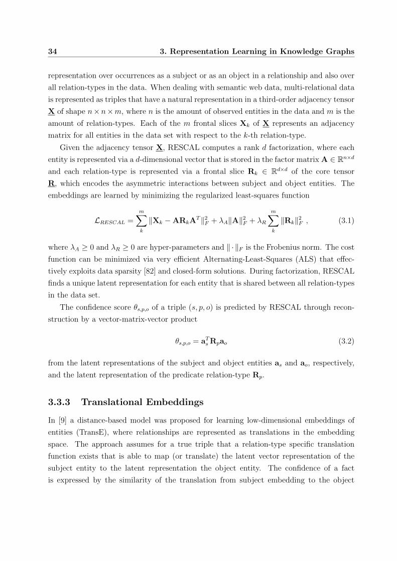
34 3. Representation Learning in Knowledge Graphs
representation over occurrences as a subject or as an object in a relationship and also over
all relation-types in the data. When dealing with semantic web data, multi-relational data
is represented as triples that have a natural representation in a third-order adjacency tensor
X of shape n×n×m, where n is the amount of observed entities in the data and m is the
amount of relation-types. Each of the m frontal slices Xk of X represents an adjacency
matrix for all entities in the data set with respect to the k-th relation-type.
Given the adjacency tensor X, RESCAL computes a rank d factorization, where each
entity is represented via a d-dimensional vector that is stored in the factor matrix A ∈ Rn×d
and each relation-type is represented via a frontal slice Rk ∈ Rd×d of the core tensor
R, which encodes the asymmetric interactions between subject and object entities. The
embeddings are learned by minimizing the regularized least-squares function
LRESCAL =m∑k
‖Xk −ARkAT‖2
F + λA‖A‖2F + λR
m∑k
‖Rk‖2F , (3.1)
where λA ≥ 0 and λR ≥ 0 are hyper-parameters and ‖ ·‖F is the Frobenius norm. The cost
function can be minimized via very efficient Alternating-Least-Squares (ALS) that effec-
tively exploits data sparsity [82] and closed-form solutions. During factorization, RESCAL
finds a unique latent representation for each entity that is shared between all relation-types
in the data set.
The confidence score θs,p,o of a triple (s, p, o) is predicted by RESCAL through recon-
struction by a vector-matrix-vector product
θs,p,o = aTs Rpao (3.2)
from the latent representations of the subject and object entities as and ao, respectively,
and the latent representation of the predicate relation-type Rp.
3.3.3 Translational Embeddings
In [9] a distance-based model was proposed for learning low-dimensional embeddings of
entities (TransE), where relationships are represented as translations in the embedding
space. The approach assumes for a true triple that a relation-type specific translation
function exists that is able to map (or translate) the latent vector representation of the
subject entity to the latent representation the object entity. The confidence of a fact
is expressed by the similarity of the translation from subject embedding to the object
3.3 Statistical Modeling of Knowledge Graphs with Latent Variable Models35
embedding.
In case of TransE, the translation function is defined by a simple addition of the latent
vector representations of the subject entity as and the predicate relation-type rp. The
similarity of the translation and the object embedding is measured by the L1 or L2 distance.
TransE’s confidence θs,p,o in a triple (s, p, o) is derived by
θs,p,o = −δ(as + rp, ao), (3.3)
where δ is the L1 or the L2 distance and ao is the latent embedding for the object entity.
The embeddings are learned by minimizing the margin-based ranking cost function
LTransE =∑
(s,p,o)∈T
max{0, γ + θs′,p,o − θs,p,o}+ max{0, γ + θs,p,o′ − θs,p,o} (3.4)
with {s′, o′} ∈ E
on a set of observed training triples T through Stochastic Gradient Descent (SGD), where
γ > 0 is the margin and the corrupted entities s′ and o′ are drawn from the set of all
observed entities E . Note that subject and object entities are never replaced at the same
time. Instead, for one triple out of T two corrupted ones are sampled where either the
subject or the object entity is replaced by a random entity. During training, it is enforced
that the latent embeddings of entities have an L2 norm of 1 after each SGD iteration.
3.3.4 Google Knowledge-Vault Neural-Network
The Google Knowledge Vault project [25] pursues an automatic construction of a high
quality knowledge graph. In this regard a multiway neural network (mwNN) based model
for predicting prior probabilities for triples from existing knowledge graph data was pro-
posed to support triple extraction from unstructured web documents. The confidence value
θs,p,o for a target triple (s, p, o) is predicted by
θs,p,o = σ(βTφ (W [as, rp, ao])) (3.5)
where φ() is a nonlinear function like e.g. tanh, as and ao describe the latent embedding
vectors for the subject and object entities and rp is the latent embedding vector for the
predicate relation-type p. [as, rp, ao] ∈ R3d×1 is a column vector that stacks the three
embeddings on top of each other. W and β are neural network weights and σ() denotes
36 3. Representation Learning in Knowledge Graphs
the sigmoid function. The model is trained by minimizing the Bernoulli cost-function
LmwNN = −∑
(s,p,o)∈T
log θs,p,o −c∑
o′∈E
log(1− θs,p,o′) (3.6)
through SGD, where c denotes the number of corrupted triples sampled under a local
closed-world assumption as defined by [25], where only the object entity is corrupted by
a random entity drawn from E . Note that we only sample observed triples (which are
assumed to be true) and the corrupted triples generated from these are all treated as
negative evidence.
Chapter 4Applying Latent Variable Models to Large
Knowledge Graphs
In this chapter we study the different latent variable models introduced in Chapter 3.3
with regard to their application to large knowledge graphs. Due to their size, large knowl-
edge graphs require to constrain the complexity of the latent embeddings for entities and
relation-types exploited by these models. These constraints are mostly disregarded in the
discussions and conclusions of related literature, but are very important to consider when
selecting and applying these models to large data sets. In the following sections we will
give more details to these constraints and describe their impact on TransE, RESCAL and
mwNN. We further simulate the application of these models (link-prediction) on large
knowledge graphs based on various data sets, in order evaluate their performance in such
a setting.
Own contributions in this chapter are part of our prior work on the contributions
described in Chapter 5. The experimental results regarding the area under precision recall
curve (AUPRC) and area under receiver characteristic (AUROC) scores shown in Tables
4.3, 4.4 and 4.5 have been published in
[54] Denis Krompaß, Stephan Baier and Volker Tresp. Type-Constrained Representa-
tion Learning in Knowledge-Graphs. 14th International Semantic Web Conference
(ISWC). 2015
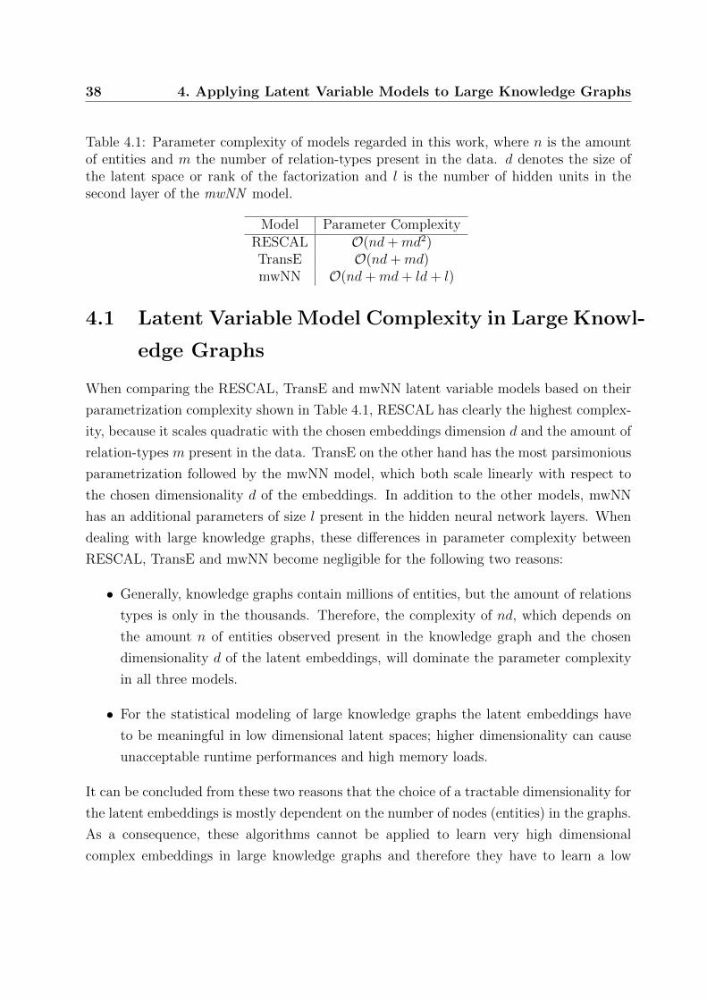
38 4. Applying Latent Variable Models to Large Knowledge Graphs
Table 4.1: Parameter complexity of models regarded in this work, where n is the amountof entities and m the number of relation-types present in the data. d denotes the size ofthe latent space or rank of the factorization and l is the number of hidden units in thesecond layer of the mwNN model.
Model Parameter ComplexityRESCAL O(nd+md2)TransE O(nd+md)mwNN O(nd+md+ ld+ l)
4.1 Latent Variable Model Complexity in Large Knowl-
edge Graphs
When comparing the RESCAL, TransE and mwNN latent variable models based on their
parametrization complexity shown in Table 4.1, RESCAL has clearly the highest complex-
ity, because it scales quadratic with the chosen embeddings dimension d and the amount of
relation-types m present in the data. TransE on the other hand has the most parsimonious
parametrization followed by the mwNN model, which both scale linearly with respect to
the chosen dimensionality d of the embeddings. In addition to the other models, mwNN
has an additional parameters of size l present in the hidden neural network layers. When
dealing with large knowledge graphs, these differences in parameter complexity between
RESCAL, TransE and mwNN become negligible for the following two reasons:
• Generally, knowledge graphs contain millions of entities, but the amount of relations
types is only in the thousands. Therefore, the complexity of nd, which depends on
the amount n of entities observed present in the knowledge graph and the chosen
dimensionality d of the latent embeddings, will dominate the parameter complexity
in all three models.
• For the statistical modeling of large knowledge graphs the latent embeddings have
to be meaningful in low dimensional latent spaces; higher dimensionality can cause
unacceptable runtime performances and high memory loads.
It can be concluded from these two reasons that the choice of a tractable dimensionality for
the latent embeddings is mostly dependent on the number of nodes (entities) in the graphs.
As a consequence, these algorithms cannot be applied to learn very high dimensional
complex embeddings in large knowledge graphs and therefore they have to learn a low
4.2 Simulating Large Scale Conditions 39
number of very meaningful factors that explain the data. Since all models have to exploit
a similar dimensionality for the learned embeddings, the training time and expressiveness of
the model will mainly dependent on the optimization algorithm and modeling assumptions.
ALS optimized models, i.e. RESCAL, that can exploit closed form solutions allow a faster
model optimization than models that exploit stochastic gradient descent. However, as a
drawback, the choice of the target loss function is limited to a Gaussian likelihood function.
In addition, a closed-world assumption has to be used, which does not consider the notion
of missing data. In chapter 5 we will show how local closed-world-assumptions can be
exploited to increase RESCAL’s capability to consider missing data in its closed form
solution updates exploited in ALS (see also [56, 54]). TransE and mwNN are optimized
through stochastic gradient descent, which generally lead to longer training times. On the
other hand, SGD allows a more careful loss function design which often better represents the
underlying assumptions observed in the data regarding missing values and the distribution
of the data.
4.2 Simulating Large Scale Conditions
In this section we describe our experimental setup in which we simulate the application of
RESCAL, TransE and mwNN to large knowledge graphs. Our experimental setup covers
two important aspects:
• We test these models with reasonably low complexity levels, meaning that we enforce
low dimensional latent embeddings for entities and relation-types which simulates
their application to very large data sets where high dimensional embeddings are
intractable. In [25] for example, a latent embedding length (parameter d in Chapter
3.3) of 60 was used.
• We extracted diverse data sets from instances of the Linked-Open Data Cloud,
namely Freebase, YAGO and DBpedia, because it is expected that the needed com-
plexity of the models is also dependent on the particular data set the models are
applied to. From these knowledge graphs we constructed data sets that will be used
as representatives for general purpose knowledge graphs that cover a wide range of
relation-types from a diverse set of domains, domain focused knowledge graphs with
a specific (smaller) amount of entity classes and relation-types, and high quality
knowledge graphs.
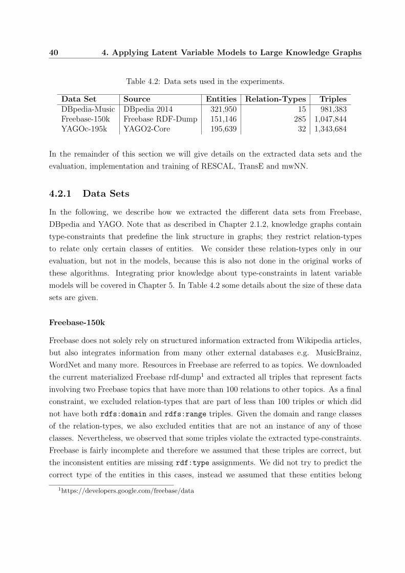
40 4. Applying Latent Variable Models to Large Knowledge Graphs
Table 4.2: Data sets used in the experiments.
Data Set Source Entities Relation-Types TriplesDBpedia-Music DBpedia 2014 321,950 15 981,383Freebase-150k Freebase RDF-Dump 151,146 285 1,047,844YAGOc-195k YAGO2-Core 195,639 32 1,343,684
In the remainder of this section we will give details on the extracted data sets and the
evaluation, implementation and training of RESCAL, TransE and mwNN.
4.2.1 Data Sets
In the following, we describe how we extracted the different data sets from Freebase,
DBpedia and YAGO. Note that as described in Chapter 2.1.2, knowledge graphs contain
type-constraints that predefine the link structure in graphs; they restrict relation-types
to relate only certain classes of entities. We consider these relation-types only in our
evaluation, but not in the models, because this is also not done in the original works of
these algorithms. Integrating prior knowledge about type-constraints in latent variable
models will be covered in Chapter 5. In Table 4.2 some details about the size of these data
sets are given.
Freebase-150k
Freebase does not solely rely on structured information extracted from Wikipedia articles,
but also integrates information from many other external databases e.g. MusicBrainz,
WordNet and many more. Resources in Freebase are referred to as topics. We downloaded
the current materialized Freebase rdf-dump1 and extracted all triples that represent facts
involving two Freebase topics that have more than 100 relations to other topics. As a final
constraint, we excluded relation-types that are part of less than 100 triples or which did
not have both rdfs:domain and rdfs:range triples. Given the domain and range classes
of the relation-types, we also excluded entities that are not an instance of any of those
classes. Nevertheless, we observed that some triples violate the extracted type-constraints.
Freebase is fairly incomplete and therefore we assumed that these triples are correct, but
the inconsistent entities are missing rdf:type assignments. We did not try to predict the
correct type of the entities in this cases, instead we assumed that these entities belong
1https://developers.google.com/freebase/data
4.2 Simulating Large Scale Conditions 41
to the domain or range of the relation-type where the inconsistency was observed. More
technically, if we observe for a triple (s, p, o) that e.g. subject entity s disagrees with the
type-constraints of relation-type p, then we simply add the index of entity s to the index
vector domainp, which is used to extract all entities from E that belong to the domain
of relation-type p. This data set will simulate a general purpose knowledge graph in our
experiments.
DBpedia-Music
DBpedia contains the structured information extracted from Wikipedia Infoboxes. For
the DBpedia-Music data set, we downloaded the owl-ontology, mapping-based-properties
(cleaned), mapping-based-types and heuristics from the canonicalized data sets of the
current release of DBpedia2. We extracted triples from 15 pre-selected Object-Properties;
musicalBand, musicalArtist, musicBy, musicSubgenre, derivative, stylisticOrigin,
associatedBand, associatedMusicalArtist, recordedIn, musicFusionGenre, music-
Composer, artist, bandMember, formerBandMember, genre, where genre has been ex-
tracted to include only those entities that were covered by the other object-properties to
restrict it to musical genres. We discarded all triples of entities that occurred less than
twice and for all of the remaining entities that are not assigned to any class, we assigned
them to owl#Thing. The rdfs:domain and rdfs:range concepts for the above relation-
types were extracted from the DBpedia ontology, where we defined the domain or range of
a relation-type as owl#Thing if absent. Similar to the Freebase data set, we also observed
that some triples disagree with the domain and range constraints of the corresponding
relation-type and treated them similarly to the Freebase data set. In our experiments, this
data set will simulate a domain specific knowledge graph.
YAGOc-195k
YAGO (Yet Another Great Ontology) is an automatically generated high quality knowledge
graph that combines the information richness of Wikipedia Infoboxes and its category
system with the clean taxonomy of WordNet. We downloaded the core data set from the
YAGO website3 that contains facts between YAGO-instances. In addition, we downloaded
the schema information including the rdf:type, rdfs:range and rdfs:domain triples.4
2http://wiki.dbpedia.org/Downloads20143http://www.mpi-inf.mpg.de/departments/databases-and-information-systems/research/yago-
naga/yago/downloads/4yagoSchema and yagoTransitiveType
42 4. Applying Latent Variable Models to Large Knowledge Graphs
We only included entities that had at least 5 occurrences and that share the types used
in the rdfs:domain and rdfs:range triples. We also excluded relation-types for which
less than 100 triples could be observed after pruning the entities could be observed. In
contrast to the other two data sets, all triples agreed with the domain and range constraints
of the relation-types and therefore no further editing of the data set was needed. This
YAGO subsample will be used as representative for a high quality knowledge graph in our
experiments.
4.2.2 Evaluation Procedure
We evaluate RESCAL, TransE and mwNN on link prediction tasks, where we delete triples
from the data sets and try to re-predict them without considering them during model
training. For model training and evaluation we split the triples of the data sets into
three sets, where 20% of the triples were taken as holdout set, 10% as validation set for
hyper-parameter tuning and the remaining 70% served as training set5. In case of the
validation and holdout set, we sampled 10 times as many negative triples for evaluation,
where the negative triples were drawn such that they did not violate the given domain and
range constraints of the knowledge graph. Also, the negative evidence of the holdout and
validation set are not overlapping. In knowledge graph data, we are generally dealing with
a strongly skewed ratio of observed and unobserved triples, through this sampling we try
to mimic this effect to some extent since it is intractable to sample all unobserved triples.
After deriving the best hyper-parameter settings for all models, we trained all models with
these settings using both the training and the validation set to predict the holdout set (20%
of triples). We report the Area Under Precision Recall Curve (AUPRC) for all models. In
addition, we provide the Area Under Receiver Operating Characteristic Curve (AUROC),
because it is widely used for this problem even though it is not well suited as evaluation
measure in these tasks due to the imbalance of (assumed) false and true triples.6 The
discussions and conclusions will be primarily based on the AUPRC results.
We also evaluate the training time of the models, where we measure the runtime in
seconds for model training and the number of epochs used until convergence when trained
on the validation and training set (80% of triples). In addition we give the mean time per
training epoch and the corresponding standard-deviation for better comparison.
5Additional 5% of the training set were used for early stopping.6AUROC includes the false-positive rate which relies on the amount of true-negatives that is generally
high in these kind of data sets, often leading often to misleading high scores.
4.2 Simulating Large Scale Conditions 43
4.2.3 Implementation and Model Training Details
All models were implemented in Python using in part Theano [5]. Theano code for TransE
is provided by the authors, but we replaced some parts of the original implementation that
allowed a significantly faster training.7 We made sure that our implementation achieved
very similar results to the original model on a smaller data set8 (Results not shown).
The Google Knowledge-Vault multiway neural network (mwNN) was also implemented
in Theano. Since there are not many details on model training in the corresponding work
[25], we added elastic-net regularization combined with DropConnect [111] on the network
weights and optimized the cost function using mini-batch adaptive gradient descent [26].
We randomly initialized the weights by drawing from a zero mean normal distribution
where we treat the standard deviation as an additional hyper-parameter. The corrupted
triples were sampled with respect to the local closed-world assumption discussed in [25].
We fixed the amount of corrupted triples per training example to five.9
For RESCAL, we used the ALS implementation provided by the author10, but extended
it in such a way that it supports a more scalable early stopping criteria based on a small
validation set.
For hyper-parameter tuning, all models were trained for a maximum of 50 epochs and
for the final evaluation on the holdout set for a maximum of 200 epochs. For all models,
we sampled 5% of the training data as validation set and computed the change in AUPRC
for early stopping on this set. For ALS, we stopped training if the AUPRC score did not
increase more than 1E−4 for five epochs in a row and kept the best known configuration.
In case of the SGD optimized models, we computed the AUPRC twice in an epoch and
stopped training after the AUPRC score has also not increased 10 times in a row for 1E−4.
All models were trained with an Intel Xeon E5-2680 v2 (Amazon EC2 c3 instance)
using 4 threads (OpenBLAS).
7Slower runtime is mainly caused by the ranking function used for calculating the validation error, butthe consideration of trivial zero gradients during the SGD-updates also caused slowdowns.
8http://alchemy.cs.washington.edu/data/cora/9We tried different amounts of corrupted triples and five gave the most stable results across all data
sets.10https://github.com/mnick/scikit-tensor
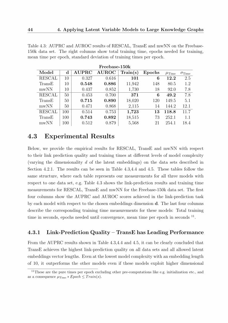
44 4. Applying Latent Variable Models to Large Knowledge Graphs
Table 4.3: AUPRC and AUROC results of RESCAL, TransE and mwNN on the Freebase-150k data set. The right columns show total training time, epochs needed for training,mean time per epoch, standard deviation of training times per epoch.
Freebase-150kModel d AUPRC AUROC Train(s) Epochs µTime σTime
RESCAL 10 0.327 0.616 101 6 12.2 2.5TransE 10 0.548 0.886 11,942 148 80.5 1.2mwNN 10 0.437 0.852 1,730 18 92.0 7.8RESCAL 50 0.453 0.700 371 6 49.2 7.8TransE 50 0.715 0.890 18,020 120 149.5 5.1mwNN 50 0.471 0.868 2,115 14 144.2 12.1RESCAL 100 0.514 0.753 1,723 13 118.8 11.7TransE 100 0.743 0.892 18,515 73 252.1 1.1mwNN 100 0.512 0.879 5,568 21 254.1 18.4
4.3 Experimental Results
Below, we provide the empirical results for RESCAL, TransE and mwNN with respect
to their link prediction quality and training times at different levels of model complexity
(varying the dimensionality d of the latent embeddings) on the data sets described in
Section 4.2.1. The results can be seen in Table 4.3,4.4 and 4.5. These tables follow the
same structure, where each table represents our measurements for all three models with
respect to one data set, e.g. Table 4.3 shows the link-prediction results and training time
measurements for RESCAL, TransE and mwNN for the Freebase-150k data set. The first
four columns show the AUPRC and AUROC scores achieved in the link-prediction task
by each model with respect to the chosen embeddings dimension d. The last four columns
describe the corresponding training time measurements for these models: Total training
time in seconds, epochs needed until convergence, mean time per epoch in seconds 11.
4.3.1 Link-Prediction Quality – TransE has Leading Performance
From the AUPRC results shown in Table 4.3,4.4 and 4.5, it can be clearly concluded that
TransE achieves the highest link-prediction quality on all data sets and all allowed latent
embeddings vector lengths. Even at the lowest model complexity with an embedding length
of 10, it outperforms the other models even if these models exploit higher dimensional
11These are the pure times per epoch excluding other pre-computations like e.g. initialization etc., andas a consequence µTime ∗ Epoch ≤ Train(s).
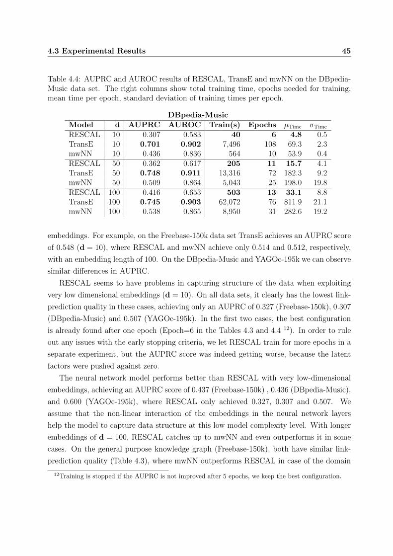
4.3 Experimental Results 45
Table 4.4: AUPRC and AUROC results of RESCAL, TransE and mwNN on the DBpedia-Music data set. The right columns show total training time, epochs needed for training,mean time per epoch, standard deviation of training times per epoch.
DBpedia-MusicModel d AUPRC AUROC Train(s) Epochs µTime σTime
RESCAL 10 0.307 0.583 40 6 4.8 0.5TransE 10 0.701 0.902 7,496 108 69.3 2.3mwNN 10 0.436 0.836 564 10 53.9 0.4RESCAL 50 0.362 0.617 205 11 15.7 4.1TransE 50 0.748 0.911 13,316 72 182.3 9.2mwNN 50 0.509 0.864 5,043 25 198.0 19.8RESCAL 100 0.416 0.653 503 13 33.1 8.8TransE 100 0.745 0.903 62,072 76 811.9 21.1mwNN 100 0.538 0.865 8,950 31 282.6 19.2
embeddings. For example, on the Freebase-150k data set TransE achieves an AUPRC score
of 0.548 (d = 10), where RESCAL and mwNN achieve only 0.514 and 0.512, respectively,
with an embedding length of 100. On the DBpedia-Music and YAGOc-195k we can observe
similar differences in AUPRC.
RESCAL seems to have problems in capturing structure of the data when exploiting
very low dimensional embeddings (d = 10). On all data sets, it clearly has the lowest link-
prediction quality in these cases, achieving only an AUPRC of 0.327 (Freebase-150k), 0.307
(DBpedia-Music) and 0.507 (YAGOc-195k). In the first two cases, the best configuration
is already found after one epoch (Epoch=6 in the Tables 4.3 and 4.4 12). In order to rule
out any issues with the early stopping criteria, we let RESCAL train for more epochs in a
separate experiment, but the AUPRC score was indeed getting worse, because the latent
factors were pushed against zero.
The neural network model performs better than RESCAL with very low-dimensional
embeddings, achieving an AUPRC score of 0.437 (Freebase-150k) , 0.436 (DBpedia-Music),
and 0.600 (YAGOc-195k), where RESCAL only achieved 0.327, 0.307 and 0.507. We
assume that the non-linear interaction of the embeddings in the neural network layers
help the model to capture data structure at this low model complexity level. With longer
embeddings of d = 100, RESCAL catches up to mwNN and even outperforms it in some
cases. On the general purpose knowledge graph (Freebase-150k), both have similar link-
prediction quality (Table 4.3), where mwNN outperforms RESCAL in case of the domain
12Training is stopped if the AUPRC is not improved after 5 epochs, we keep the best configuration.
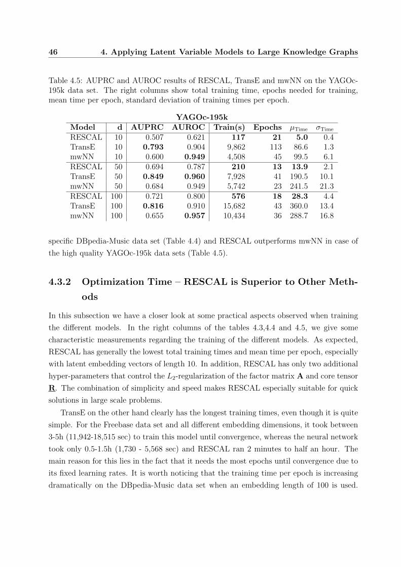
46 4. Applying Latent Variable Models to Large Knowledge Graphs
Table 4.5: AUPRC and AUROC results of RESCAL, TransE and mwNN on the YAGOc-195k data set. The right columns show total training time, epochs needed for training,mean time per epoch, standard deviation of training times per epoch.
YAGOc-195kModel d AUPRC AUROC Train(s) Epochs µTime σTime
RESCAL 10 0.507 0.621 117 21 5.0 0.4TransE 10 0.793 0.904 9,862 113 86.6 1.3mwNN 10 0.600 0.949 4,508 45 99.5 6.1RESCAL 50 0.694 0.787 210 13 13.9 2.1TransE 50 0.849 0.960 7,928 41 190.5 10.1mwNN 50 0.684 0.949 5,742 23 241.5 21.3RESCAL 100 0.721 0.800 576 18 28.3 4.4TransE 100 0.816 0.910 15,682 43 360.0 13.4mwNN 100 0.655 0.957 10,434 36 288.7 16.8
specific DBpedia-Music data set (Table 4.4) and RESCAL outperforms mwNN in case of
the high quality YAGOc-195k data sets (Table 4.5).
4.3.2 Optimization Time – RESCAL is Superior to Other Meth-
ods
In this subsection we have a closer look at some practical aspects observed when training
the different models. In the right columns of the tables 4.3,4.4 and 4.5, we give some
characteristic measurements regarding the training of the different models. As expected,
RESCAL has generally the lowest total training times and mean time per epoch, especially
with latent embedding vectors of length 10. In addition, RESCAL has only two additional
hyper-parameters that control the L2-regularization of the factor matrix A and core tensor
R. The combination of simplicity and speed makes RESCAL especially suitable for quick
solutions in large scale problems.
TransE on the other hand clearly has the longest training times, even though it is quite
simple. For the Freebase data set and all different embedding dimensions, it took between
3-5h (11,942-18,515 sec) to train this model until convergence, whereas the neural network
took only 0.5-1.5h (1,730 - 5,568 sec) and RESCAL ran 2 minutes to half an hour. The
main reason for this lies in the fact that it needs the most epochs until convergence due to
its fixed learning rates. It is worth noticing that the training time per epoch is increasing
dramatically on the DBpedia-Music data set when an embedding length of 100 is used.
4.4 Related Work 47
The DBpedia-Music data set has the most entities (321,950) and TransE seems to be more
sensitive to an increase in the size of entities. We profiled the code to ensure that this
increase in time was not caused by some inefficient code snippet and observed that the
main part of the runtime is indeed spent in the gradient calculation. Furthermore, we
found this model quite straight-forward to tune (only three additional hyper-parameters),
but its long training times limit its applicability to very large data sets. Note that our
implementation of this models is already magnitudes faster than the original code provided
by the authors, which took over a day to converge on these data sets.
In exception to the previously mentioned case where TransE’s training time per epoch
dramatically increased on the DBpedia-Music data set, the mwNN model has similar train-
ing times per epoch as TransE. However, the total training time of mwNN is significantly
lower since it needs significantly less epochs to convergence due to the adaptive gradient
optimization. As a drawback, we found this model quite hard to tune, because it has a
multitude of hyper-parameters. We clearly spent the most effort here.
4.4 Related Work
Tensors have been applied to Web analysis in [52] and for ranking predictions in the
Semantic Web in [35]. [90] applied tensor models to rating predictions. Using factorization
approaches to predict ground atoms was pioneered in [104]; [82], [113], [11], and [50]
applied tensor models for this task, where [82] introduced the RESCAL model. [94]
applied matrix factorization for relation extraction in universal schemas. The RESCAL
model has been the basis of multiple recently published works: [55] introduced non-negative
constraints, [81] presented a logistic factorization and [50] explicitly models the 2nd and
3rd order interactions.
[99] recently proposed a neural tensor network which we did not consider in our study
since it was observed that it does not scale to larger data sets [17, 25]. Instead we exploit a
less complex and more scalable neural network model proposed in [25] which could achieve
comparable results to the neural tensor network of [99].
[12] proposed the Semantic Matching Energy model (SME), which was later refined and
improved in scalability by the translational embeddings model (TransE) introduced in [9].
Entities and relation-types are represented by latent embedding vectors in these models
and the score of a triple is measured in terms of a distance-based similarity measure as mo-
tivated by [74, 73]. TransE [9] has been he target of other recent research activities. [114]
48 4. Applying Latent Variable Models to Large Knowledge Graphs
proposed a framework for relationship modeling that combines aspects of TransE and the
neural tensor network proposed in [99]. [112] proposed TransH which improves TransE’s
capability to model reflexive one-to-many, many-to-one and many-to-many relation-types
by introducing a relation-type-specific hyperplane where the translation is performed. This
work has been further extended in [67] by introducing TransR which separates representa-
tions of entities and relation-types in different spaces, where the translation is performed in
the relation-space. An extensive review on representation learning with knowledge graphs
can be found in [80].
Latent variable methods have been combined with graph-feature models which lead to
an increase of prediction quality [25] and a decrease of model complexity [79]. Further,
it has been shown in [54] that the prediction quality of latent variable models, such as
RESCAL, TransE and the neural network used in the Google Knowledge Vault system, can
also be significantly improved at lower model complexities by integrating prior knowledge
on relation-types, i.e. type-constraints extracted from the knowledge graph schema.
General methods for link-prediction also include Markov-Logic-Networks [92] which
have a limited scalability and random walk algorithms like the path ranking algorithm [60].
4.5 Conclusion
For the statistical modeling of large knowledge graphs, latent variable models require to
capture the dependencies in the graph within low dimensional latent embeddings of entities
and relation-types, since high dimensional embeddings can cause intractable training times
and memory loads. As an example, the embeddings matrix for the whole of Freebase (∼ 40
million entities, i.e. topics) will consume 16 TB of memory if an embedding length of
100,000 would be chosen (considering single precision floats). The computational costs of
such huge embedding matrices will be tremendous.
From the experimental results discussed in Section 4.3.1, we can conclude that TransE
is most capable of learning meaningful low dimensional embeddings, but with the price
of significantly higher training times than RESCAL. RESCAL on the other hand has a
significantly worse link-prediction quality than TransE when exploiting very low dimen-
sional embeddings, but is optimized extremely fast. Opposing these two extremes, one
difference becomes directly apparent: the way these models handle missing data. TransE
optimizes a max-margin ranking loss function that considers every triple as missing that
is not observed in the data. Therefore, the loss function focuses on highlighting the true
4.5 Conclusion 49
triples in the data. RESCAL on the other hand uses a closed-world assumption. RESCAL
factorizes a large third order tensor and optimizes a reconstruction penalty that considers
all possible combinations of triples in the data in every update. It is not surprising that,
due to the overwhelming amount of assumed negative evidence in the data, the reconstruc-
tion error is best minimized by approximating a tensor with almost no signals (everything
is zero) if a low amount of parameters is available. The mwNN model is in the middle of
the other two models in terms of prediction quality when exploiting very low dimensional
embeddings, probably due to its local closed-world assumption that includes aspects of
both approaches. In the case of RESCAL or mwNN there have been extensions proposed
that combine them with graph feature models to increase their link-prediction capabilities
with lower dimensional embeddings [79, 25].
However, even though the aspect of missing data seems a plausible explanation for
the observed differences in quality of the prediction results between all three models, it
masks one important aspect of knowledge graphs that is not considered by any of these
methods, –a knowledge graph is not a complete graph–. In addition to true, missing and
(assumed) false triples we have to deal with the fact that there are combinations of entities
and relation-types that should not occur at all, because they do not make any sense.
The differentiation from these “impossible” triples is provided through type-constraints on
relation-types (see Chapter 2.1.2). Incorporating this kind of prior knowledge on the graph
structure dramatically decreases the amount of possible worlds the latent variable models
have to consider when modeling knowledge graphs. In the next chapter we will show how
this prior knowledge can be integrated in latent variable models and study their general
value for the statistical modeling of knowledge graphs with latent variable models.
50 4. Applying Latent Variable Models to Large Knowledge Graphs
Chapter 5Exploiting Prior Knowledge On
Relation-Type Semantics
We have illustrated in Chapter 2.1.2 that besides storing facts about the world, schema-
based knowledge graphs are backed by rich semantic descriptions of entities and relation-
types that allow machines to understand the notion of things and their semantic rela-
tionships. Generally, entities in knowledge graphs like DBpedia, Freebase or YAGO are
assigned to one or multiple predefined classes (or types) that are organized in an often
hierarchical ontology. These assignments represent for example the knowledge that the en-
tity Albert Einstein is a person and therefore allow a semantic description of the entities
contained in the knowledge graph. The organization of entities in semantically meaningful
classes further permits a semantic definition of relation-types. The RDF-Schema offers
among others the concepts rdfs:domain and rdfs:range for this purpose. Annotations
that describe relation-type semantics provide valuable information to machines, e.g. that
the marriedTo relation-type should relate only instances of the class person.
In this chapter we study the general value of prior knowledge about the semantics of
relation-types and entities for the statistical modeling of knowledge graphs with latent
variable models. We show how the annotated semantics provided by the rdfs:domain
and rdfs:range concepts can be effectively exploited in latent variable models, thereby
improving the link prediction quality significantly on various data sets.
Additionally, we address the issue that type-constraints can also suffer from incomplete-
ness; rdfs:domain or rdfs:range concepts are absent in the schema or the entities miss
proper typing even after materialization. In this regard, we motivate and study a local
closed-world assumption that approximates the semantics of relation-types solely based
52 5. Exploiting Prior Knowledge On Relation-Type Semantics
on observed triples in the graph. We provide empirical proof that this prior assumption
on relation-types generally improves link-prediction quality in case proper type-constraints
are absent or fuzzy.
This chapter is structured as follows: In the following section, we extend RESCAL’s
efficient optimization algorithm such that type-constraints are considered without loosing
the its great scalability properties. Furthermore, we discuss a series of proof of concept
experiments which show that RESCAL benefits to a large extent from the integration
of prior knowledge on relation-types. The integration of prior knowledge about type-
constraints is not limited to RESCAL, but can also be integrated in the stochastic gradient
optimized models exploited by TransE and mwNN. We show how this can be accomplished
in in Section 5.2. In Section 5.3 we motivate and describe a local closed-world assumption
on relation-types that can be exploited by latent variable models in case proper type-
constraints are absent or fuzzy. In the final part of this chapter (Section 5.4) , we analyze
the general value of type-constraints and the proposed local closed-world assumption in
more detail based on extensive experiments on all models and various representative data
sets. We provide related work in Section 5.5 and conclude in Section 5.6.
Own contributions in this chapter are published in
[56] Denis Krompaß, Maximilian Nickel and Volker Tresp. Large-Scale Factorization of
Type-Constrained Multi-Relational Data. International Conference on Data Science
and Advanced Analytics (DSAA2014), 2014.
[54] Denis Krompaß, Stephan Baier and Voker Tresp. Type-Constrained Representation
Learning in Knowledge-Graphs. In Proceedings of the 14th International Semantic
Web Conference (ISWC), 2015
where Section 5.1 and Section 5.3 cover the main contributions published in [56] but with
improved notation. The contributions published in [54] are depicted in Section 5.2 and
Section 5.4.
5.1 Type-Constrained Alternating Least-Squares for
RESCAL
RESCAL as proposed by [82][83] does not consider or support type-constraints, but posts
a closed-word assumption on the complete adjacency tensor. A closed-world assumption
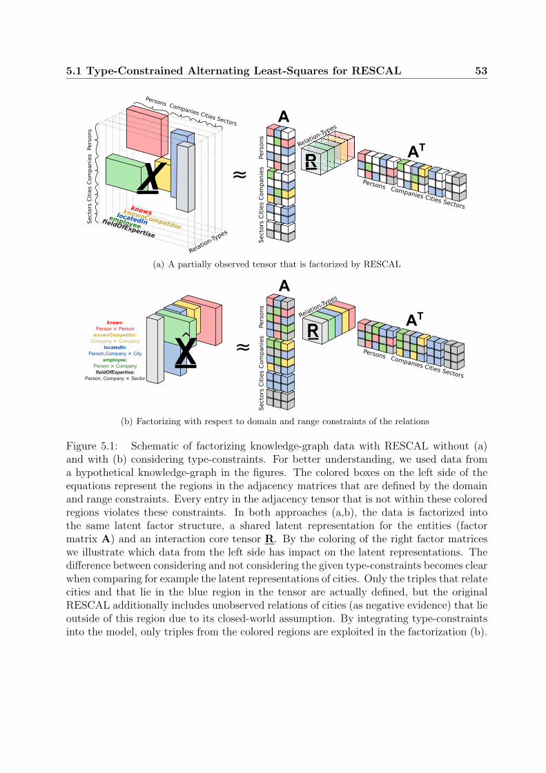
5.1 Type-Constrained Alternating Least-Squares for RESCAL 53
≈
Persons Companies Cities SectorsA
AT
Secto
rs C
itie
s C
om
panie
s
Pers
ons
Persons Companies Cities Sectors
Secto
rs C
itie
s C
om
panie
s
Pers
ons
fieldOfExpertise
employee
locatedIn
knownCompetitor
knows
Relation-Ty
pes
Relation-Ty
pes
X
(a) A partially observed tensor that is factorized by RESCAL
R≈X
A
ATknows:
Person ⨯ Person
knownCompetitor:
Company ⨯ Company
locatedIn:
Person,Company ⨯ City
employee:
Person ⨯ Company
fieldOfExpertise:
Person, Company ⨯ Sector
^Persons Companies Cities Sectors
Secto
rs C
itie
s C
om
panie
s
Pers
ons
Relation-Ty
pes
(b) Factorizing with respect to domain and range constraints of the relations
Figure 5.1: Schematic of factorizing knowledge-graph data with RESCAL without (a)and with (b) considering type-constraints. For better understanding, we used data froma hypothetical knowledge-graph in the figures. The colored boxes on the left side of theequations represent the regions in the adjacency matrices that are defined by the domainand range constraints. Every entry in the adjacency tensor that is not within these coloredregions violates these constraints. In both approaches (a,b), the data is factorized intothe same latent factor structure, a shared latent representation for the entities (factormatrix A) and an interaction core tensor R. By the coloring of the right factor matriceswe illustrate which data from the left side has impact on the latent representations. Thedifference between considering and not considering the given type-constraints becomes clearwhen comparing for example the latent representations of cities. Only the triples that relatecities and that lie in the blue region in the tensor are actually defined, but the originalRESCAL additionally includes unobserved relations of cities (as negative evidence) that lieoutside of this region due to its closed-world assumption. By integrating type-constraintsinto the model, only triples from the colored regions are exploited in the factorization (b).
54 5. Exploiting Prior Knowledge On Relation-Type Semantics
corresponds to the assumption that an entity can be related to any other known entity in the
database. Especially in general purpose knowledge graphs such as Freebase or DBpedia
this assumption has many disadvantages. Most of the relation-types are specialized to
express relations between certain classes of entities, explicitly excluding a vast amount of
relations to other entity classes. In Figure 5.1.a we illustrate this by an example regarding
a hypothetical knowledge-graph about companies and their employees. For RESCAL,
the data is stored in a three-way adjacency tensor (Chapter 3.3.2), but in difference to
multi-relational data sets e.g. the Nations or Kinship data sets1, the different relation-
types are not always defined for all the entities. Instead, we are dealing with a partially
observed tensor where, as indicated by the colored blocks in the adjacency tensor, the
potentially observable parts are predefined through each relation-type’s type-constraints2.
For example, the relation-type knownCompetitor only relates entities of the class company
to each other (red block in last frontal slice) or the relation-typ employee relates entities
of the class company with entities of the class person (green block in second frontal slice of
tensor X in Figure 5.1.a). On the other hand, obviously meaningless relations between the
same class of entities (persons and companies) using the fieldOfExpertise relation-type
are excluded (e.g. the relation (John Smith, fieldOfExpertise, IBM)).
By ignoring prior knowledge about type-constraints all possible combinations of enti-
ties and relation-types are considered during factorization that include a vast amount of
meaningless triples. These meaningless triples have a significant impact on the embeddings
of entities and relation-types learned by RESCAL. In addition, they increase the sparsity
of the adjacency tensor by several magnitudes, what causes additional problems by its own
when factorizing the data. It is expected that the larger and heterogeneous the knowledge
graph, the more of these trivial false triples are implicitly represented in the tensor and
the more severe is the impact on the factorization and the latent embeddings.
To understand the problem in more detail, we have to take a closer look at how RESCAL
learns the embeddings during factorization. Let us consider the relation-type locatedIn
in Figure 5.1.a. The blue block in the adjacency tensor represents the triples that agree
with the type-constraints, namely entities of the classes person and company are being
related to instances of the class city. By considering the RESCAL update for the latent
1http://alchemy.cs.washington.edu/data/2Assuming a clean knowledge graph as for example YAGO where all relation-types have such constraints.
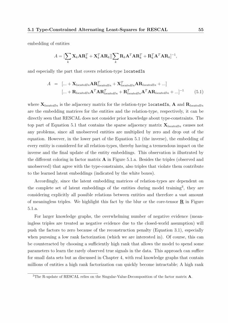
5.1 Type-Constrained Alternating Least-Squares for RESCAL 55
embedding of entities
A = [∑k
XkARTk + XT
kARk][∑k
RkATART
k + RTkATARk]
−1,
and especially the part that covers relation-type locatedIn
A = [...+ XlocatedInARTlocatedIn + XT
locatedInARlocatedIn + ...]
[...+ RlocatedInATART
locatedIn + RTlocatedInA
TARlocatedIn + ...]−1 (5.1)
where XlocatedIn is the adjacency matrix for the relation-type locatedIn, A and RlocatedIn
are the embedding matrices for the entities and the relation-type, respectively, it can be
directly seen that RESCAL does not consider prior knowledge about type-constraints. The
top part of Equation 5.1 that contains the sparse adjacency matrix XlocatedIn causes not
any problems, since all unobserved entities are multiplied by zero and drop out of the
equation. However, in the lower part of the Equation 5.1 (the inverse), the embedding of
every entity is considered for all relation-types, thereby having a tremendous impact on the
inverse and the final update of the entity embeddings. This observation is illustrated by
the different coloring in factor matrix A in Figure 5.1.a. Besides the triples (observed and
unobserved) that agree with the type-constraints, also triples that violate them contribute
to the learned latent embeddings (indicated by the white boxes).
Accordingly, since the latent embedding matrices of relation-types are dependent on
the complete set of latent embeddings of the entities during model training3, they are
considering explicitly all possible relations between entities and therefore a vast amount
of meaningless triples. We highlight this fact by the blur or the core-tensor R in Figure
5.1.a.
For larger knowledge graphs, the overwhelming number of negative evidence (mean-
ingless triples are treated as negative evidence due to the closed-world assumption) will
push the factors to zero because of the reconstruction penalty (Equation 3.1), especially
when pursuing a low rank factorization (which we are interested in). Of course, this can
be counteracted by choosing a sufficiently high rank that allows the model to spend some
parameters to learn the rarely observed true signals in the data. This approach can suffice
for small data sets but as discussed in Chapter 4, with real knowledge graphs that contain
millions of entities a high rank factorization can quickly become intractable; A high rank
3The R-update of RESCAL relies on the Singular-Value-Decomposition of the factor matrix A.
56 5. Exploiting Prior Knowledge On Relation-Type Semantics
has a dramatic impact on the runtime4 and memory consumption of RESCAL.
In order to integrate type-constraints as given by the rdfs:domain and rdfs:range
triples, we have to guarantee that all triples that violate the type-constraints are ignored
for all relation-types during factorization. In other words, for each relation-type we want
to factorize the corresponding knowledge-graph with respect to the subset of entities that
agrees with the type-constraints and suits the semantics of the corresponding relation.
Therefore, the factorization of each frontal slice of the adjacency tensor, in which each
frontal slice represents an adjacency matrix for one relation-type, might be completely
different in shape to the ones of the other frontal slices (Figure 5.1.b) because we exclude
entities. Strictly speaking, we dismiss the representation of the triples in a uniformly
shaped third-order adjacency tensor in favor of a list of frontal slices of arbitrary shape in
which each of these frontal slices explicitly excludes triples that violate the corresponding
type-constraints. Nevertheless, we want to exploit the same factorization structure than
RESCAL, but where each adjacency matrix of the relation-types only influences the latent
embeddings of a smaller subset of entities unless all entities are included in the union of
classes covered by the domain and range constraints. The goal of this approach is indicated
by the factorization in Figure 5.1.b, the latent embeddings are clean. By “clean” we mean
that no meaningless triples contribute to the latent embeddings of entities or relation-types
(no white boxes in A and no blur in core tensor R).
Factorizing the list of frontal slices efficiently can be achieved by integrating the type-
constraints directly into the RESCAL Least-Squares cost function and by exploiting a sim-
ilar Alternating Least-Squares optimization scheme. For this reason, the type-constraints
have to be encoded in a way that can be exploited by the optimization algorithm as we
will show next.
5.1.1 Additional Notation
In addition to the notation used in Chapter 3.3.1, Xk will denote the frontal-slice Xk
where only subject entities (rows) and object entities (columns) are included that agree
with the domain and range constraints of relation-type k. Additionally, we denote X[z,:]
for the indexing of multiple rows from the matrix X, where z is a vector of indices and “:”
the colon operator generally used when indexing arrays. We further denote domaink as
the sorted indices of all entities that agree with the domain constraints of relation-type k.
Accordingly, rangek denotes these indices for the range constraints of relation-type k.
4RESCAL scales cubic with the rank.
5.1 Type-Constrained Alternating Least-Squares for RESCAL 57
5.1.2 Integrating Type-Constraints into RESCAL
The integration of type-constraints in the RESCAL ALS optimization algorithm requires
a suitable representation of these type-constraints. We represent the type-constraints for
each relation-type as two vectors containing unique entity indices that we construct a
priori from the data and the given rdfs:domain and rdfs:range concepts. These entity
indices correspond to the order of entities in the latent entity embedding matrix A (and the
tensor X). We denote these vectors as domaink and rangek, where the former contains the
indices of entities that belong to classes defined by the domain and the latter to the classes
defined by the range of the relation-type k. These index vectors are exploited to extract
the sub-adjacency matrices from each frontal slice in the adjacency tensor X to construct
the previously mentioned new representation of the knowledge graph as a list of adjacency
matrices of arbitrary shape (Figure 5.1.b). By exploiting this new data representation and
the two index vectors, RESCAL’s regularized Least-Squares cost function is adapted to
L =∑k
‖Xk −A[domaink,:]RkAT[rangek,:]
‖2F + λA‖A‖2
F + λR∑k
‖Rk‖2F , (5.2)
where A represents the latent embeddings for the entities and Rk the embeddings for the
relation-type k. For each relation-type k the latent embedding matrix A is indexed by the
corresponding domain and range constraints in order to exclude all entities that disagree
with the type constraints. Xk denotes the adjacency matrix for the subgraph that agrees
with the type-constraints of relation-type k. Note that, if the adjacency matrix Xk defined
by the sub-graph of relation-type k and its type-constraints has the shape nk ×mk, then
A[domaink,:] is of shape nk × d and A[rangek,:] is of shape mk × d, where d is the dimension
of the latent embeddings (or rank of the factorization).
Even though the cost function defined in Equation 5.2 looks very similar to the cost
function of RESCAL (Equation 3.1), it contains important differences since we are actually
factorizing a list of matrices of arbitrary shapes (denoted by the “ ”) instead of uniformly
shaped frontal tensor slices. However, through the similar formulation of the optimization
problem we are still able to exploit the nice scalability properties of RESCAL. In the next
two subsections, we provide details on the ALS updates of the factor matrix A and the core
Tensor R of type-constrained RESCAL. The full algorithm is illustrated in Algorithm 1,
where domainX denotes the list of index vectors domaink and rangek for each relation-
type k present in the data (tensor X).
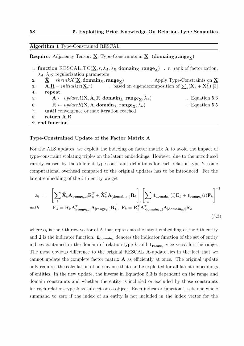
58 5. Exploiting Prior Knowledge On Relation-Type Semantics
Algorithm 1 Type-Constrained RESCAL.
Require: Adjacency Tensor: X, Type-Constraints in X: (domainX,rangeX)
1: function RESCAL TC(X, r, λA, λR,domainX, rangeX) . r: rank of factorization,λA, λR: regularization parameters
2: X = shrinkX(X,domainX, rangeX) . Apply Type-Constraints on X3: A,R = initialize(X,r) . based on eigendecomposition of
∑k(Xk + XT
k ) [3]4: repeat5: A← updateA(X,A,R,domainX, rangeX, λA) . Equation 5.3
6: R← updateR(X,A,domainX, rangeX, λR) . Equation 5.57: until convergence or max iteration reached8: return A,R9: end function
Type-Constrained Update of the Factor Matrix A
For the ALS updates, we exploit the indexing on factor matrix A to avoid the impact of
type-constraint violating triples on the latent embeddings. However, due to the introduced
variety caused by the different type-constraint definitions for each relation-type k, some
computational overhead compared to the original updates has to be introduced. For the
latent embedding of the i-th entity we get
ai =
[∑k
XkA[rangek,:]RTk + XT
kA[domaink,:]Rk
]i
[∑k
1domaink(i)Ek + 1rangek(i)Fk
]−1
with Ek = RkAT[rangek,:]
A[rangek,:]RTk , Fk = RT
kAT[domaink,:]
A[domaink,:]Rk
(5.3)
where ai is the i-th row vector of A that represents the latent embedding of the i-th entity
and 1 is the indicator function. 1domaink denotes the indicator function of the set of entity
indices contained in the domain of relation-type k and 1rangek vice versa for the range.
The most obvious difference to the original RESCAL A-update lies in the fact that we
cannot update the complete factor matrix A as efficiently at once. The original update
only requires the calculation of one inverse that can be exploited for all latent embeddings
of entities. In the new update, the inverse in Equation 5.3 is dependent on the range and
domain constraints and whether the entity is included or excluded by those constraints
for each relation-type k as subject or as object. Each indicator function 1 sets one whole
summand to zero if the index of an entity is not included in the index vector for the
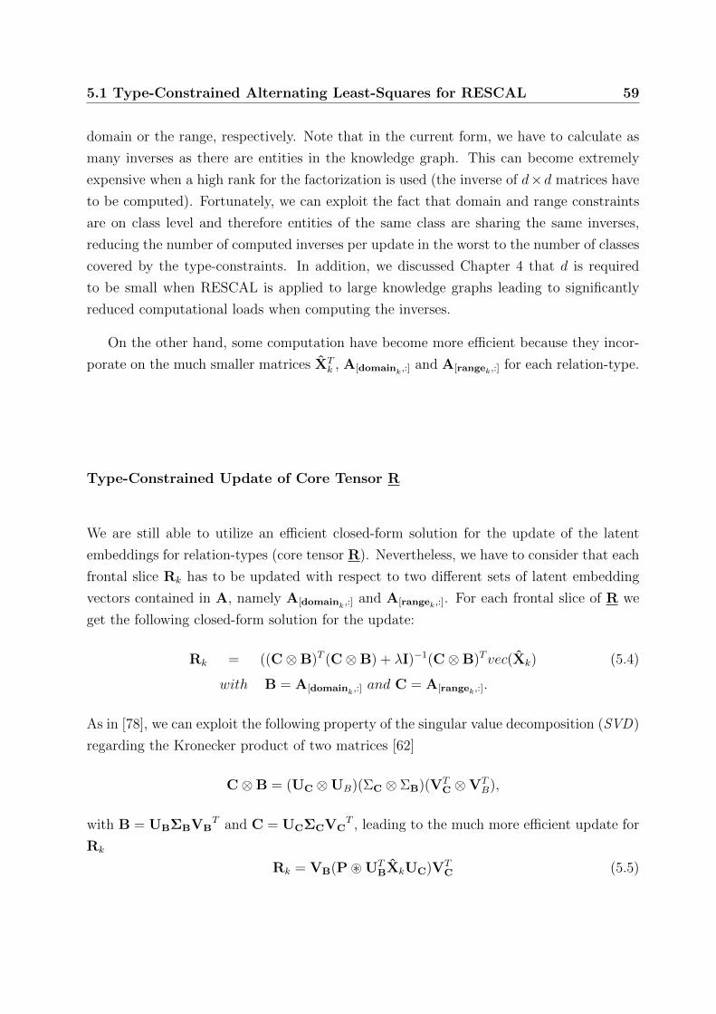
5.1 Type-Constrained Alternating Least-Squares for RESCAL 59
domain or the range, respectively. Note that in the current form, we have to calculate as
many inverses as there are entities in the knowledge graph. This can become extremely
expensive when a high rank for the factorization is used (the inverse of d×d matrices have
to be computed). Fortunately, we can exploit the fact that domain and range constraints
are on class level and therefore entities of the same class are sharing the same inverses,
reducing the number of computed inverses per update in the worst to the number of classes
covered by the type-constraints. In addition, we discussed Chapter 4 that d is required
to be small when RESCAL is applied to large knowledge graphs leading to significantly
reduced computational loads when computing the inverses.
On the other hand, some computation have become more efficient because they incor-
porate on the much smaller matrices XTk , A[domaink,:]
and A[rangek,:] for each relation-type.
Type-Constrained Update of Core Tensor R
We are still able to utilize an efficient closed-form solution for the update of the latent
embeddings for relation-types (core tensor R). Nevertheless, we have to consider that each
frontal slice Rk has to be updated with respect to two different sets of latent embedding
vectors contained in A, namely A[domaink,:]and A[rangek,:]. For each frontal slice of R we
get the following closed-form solution for the update:
Rk = ((C⊗B)T (C⊗B) + λI)−1(C⊗B)Tvec(Xk) (5.4)
with B = A[domaink,:]and C = A[rangek,:].
As in [78], we can exploit the following property of the singular value decomposition (SVD)
regarding the Kronecker product of two matrices [62]
C⊗B = (UC ⊗UB)(ΣC ⊗ ΣB)(VTC ⊗VT
B),
with B = UBΣBVBT and C = UCΣCVC
T , leading to the much more efficient update for
Rk
Rk = VB(P ~ UTBXkUC)VT
C (5.5)
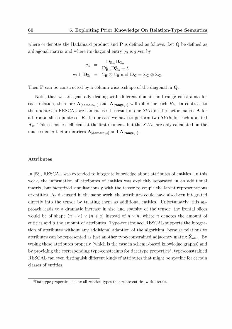
60 5. Exploiting Prior Knowledge On Relation-Type Semantics
where ~ denotes the Hadamard product and P is defined as follows: Let Q be defined as
a diagonal matrix and where its diagonal entry qii is given by
qii =DBiiDCii
D2Bii
D2Cii
+ λ
with DB = ΣB ⊗ ΣB and DC = ΣC ⊗ ΣC.
Then P can be constructed by a column-wise reshape of the diagonal in Q.
Note, that we are generally dealing with different domain and range constraints for
each relation, therefore A[domaink,:] and A[rangek,:] will differ for each Rk. In contrast to
the updates in RESCAL we cannot use the result of one SVD on the factor matrix A for
all frontal slice updates of R. In our case we have to perform two SVDs for each updated
Rk. This seems less efficient at the first moment, but the SVDs are only calculated on the
much smaller factor matrices A[domaink,:] and A[rangek,:].
Attributes
In [83], RESCAL was extended to integrate knowledge about attributes of entities. In this
work, the information of attributes of entities was explicitly separated in an additional
matrix, but factorized simultaneously with the tensor to couple the latent representations
of entities. As discussed in the same work, the attributes could have also been integrated
directly into the tensor by treating them as additional entities. Unfortunately, this ap-
proach leads to a dramatic increase in size and sparsity of the tensor; the frontal slices
would be of shape (n + a) × (n + a) instead of n × n, where n denotes the amount of
entities and a the amount of attributes. Type-constrained RESCAL supports the integra-
tion of attributes without any additional adaption of the algorithm, because relations to
attributes can be represented as just another type-constrained adjacency matrix Xattr. By
typing these attributes properly (which is the case in schema-based knowledge graphs) and
by providing the corresponding type-constraints for datatype properties5, type-constrained
RESCAL can even distinguish different kinds of attributes that might be specific for certain
classes of entities.
5Datatype properties denote all relation types that relate entities with literals.
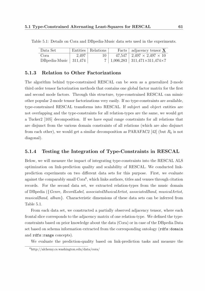
5.1 Type-Constrained Alternating Least-Squares for RESCAL 61
Table 5.1: Details on Cora and DBpedia-Music data sets used in the experiments.
Data Set Entities Relations Facts adjacency tensor XCora 2,497 10 47,547 2,497 × 2,497 × 10DBpedia-Music 311,474 7 1,006,283 311,471×311,474×7
5.1.3 Relation to Other Factorizations
The algorithm behind type-constrained RESCAL can be seen as a generalized 2-mode
third order tensor factorization methods that contains one global factor matrix for the first
and second mode factors. Through this structure, type-constrained RESCAL can mimic
other popular 2-mode tensor factorizations very easily. If no type-constraints are available,
type-constrained RESCAL transforms into RESCAL. If subject and object entities are
not overlapping and the type-constraints for all relation-types are the same, we would get
a Tucker2 [105] decomposition. If we have equal range constraints for all relations that
are disjunct from the various domain constraints of all relations (which are also disjunct
from each other), we would get a similar decomposition as PARAFAC2 [42] (but Rk is not
diagonal).
5.1.4 Testing the Integration of Type-Constraints in RESCAL
Below, we will measure the impact of integrating type-constraints into the RESCAL ALS
optimization on link-prediction quality and scalability of RESCAL. We conducted link-
prediction experiments on two different data sets for this purpose. First, we evaluate
against the comparably small Cora6, which links authors, titles and venues through citation
records. For the second data set, we extracted relation-types from the music domain
of DBpedia ({Genre, RecordLabel, associatedMusicalArtist, associatedBand, musicalArtist,
musicalBand, album}. Characteristic dimensions of these data sets can be inferred from
Table 5.1.
From each data set, we constructed a partially observed adjacency tensor, where each
frontal slice corresponds to the adjacency matrix of one relation-type. We defined the type-
constraints based on prior knowledge about the data (Cora) or in case of the DBpedia Data
set based on schema information extracted from the corresponding ontology (rdfs:domain
and rdfs:range concepts).
We evaluate the prediction-quality based on link-prediction tasks and measure the
6http://alchemy.cs.washington.edu/data/cora/
62 5. Exploiting Prior Knowledge On Relation-Type Semantics
mean Area Under Precision Recall Curve (AUPRC) score after 10 fold cross-validation.
For hyper-parameter-tuning and final evaluation, we used the same data and routine for
the 10-fold-cross-validation, but we used different seeds for splitting the data into subsets.
For the 10-fold cross-validation, we split each data set into 10 random subsets where each
subset included observed and unobserved triple which agree with the given type-constraints.
In case of the smaller Cora data set, each of these subsets included one tenth of all possible
triples sampled from the type-constrained tensor. For the DBpedia-Music data set it is
intractable to sample one tenth of the type-constrained tensor due to the huge amount
of possible triples. Instead, each of the ten subsets contained one tenth of the observed
triples and we randomly sampled 10 times as many unobserved triples and treated them as
negative evidence. We made sure that there are no overlaps between the negative evidence
of the ten subsets used for cross-validation. In each iteration of the 10-fold cross-validation
all true triples contained in one subset are removed from the tensor (set to zero) and the
remaining tensor is used for training RESCAL. After training, we predict confidences for
all triples contained in this subset and compute the AUPRC for the predicted ranking.
We measure and compare the training time in seconds for evaluating the impact of type-
constraints on the scalability of RESCAL. As discussed in Section 5.1.2, the integration of
type-constraints causes computational overhead, especially when computing the inverses in
the update of the factor-matrix A. In case of type-constrained RESCAL, the class-based
grouping of entities is included in those measurements. All experiments are conducted
with an Intel(R) Xeon(R) CPU W3520 @2.67GHz. In all experiments, RESCAL and
Type-Constrained RESCAL were trained for 20 epochs (iterations) of Alternating Least-
Squares.
Link-Prediction on Cora
With (RESCAL+TC, blue) and without (RESCAL, red) considering type-constraints,
RESCAL performs comparable well on the Cora data set (Figure 5.4.a). Both achieve
a maximum score of approx. 0.96 in AUPRC at a rank of 500 (Random: 0.013). By
considering type-constraints, it can be observed that the prediction quality increases much
faster at lower ranks up to 100. Both approaches achieve similar bad results at a rank of
one (0.11 in AUPRC), but for a rank of 25 the integration of type-constraints pays already
off, improving the link-prediction quality about 21% in AUPRC from 0.66 to 0.8. At a
rank of 100, RESCAL with type-constraints reaches already almost its maximum score of
0.96 whereas the original RESCAL algorithm achieves only 0.89 and needs an four-fold
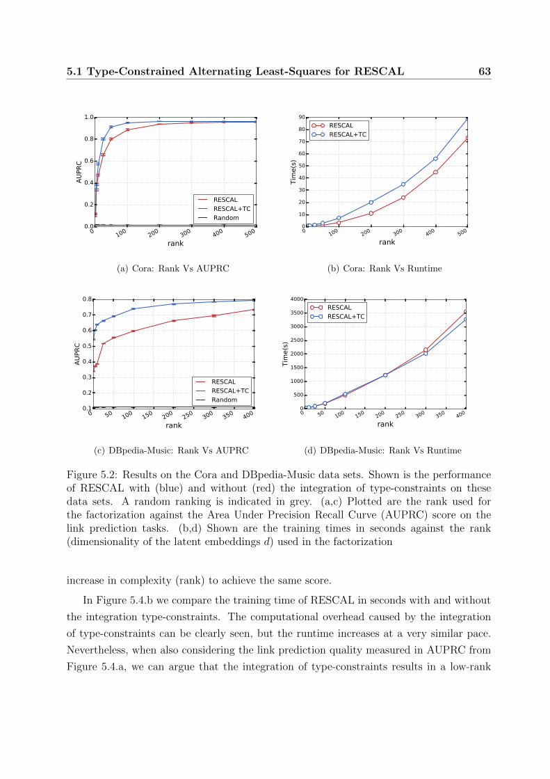
5.1 Type-Constrained Alternating Least-Squares for RESCAL 63
0100
200
300
400
500
rank
0.0
0.2
0.4
0.6
0.8
1.0
AUPRC
RESCAL
RESCAL+TC
Random
(a) Cora: Rank Vs AUPRC
0100
200
300
400
500
rank
0
10
20
30
40
50
60
70
80
90
Tim
e(s)
RESCAL
RESCAL+TC
(b) Cora: Rank Vs Runtime
0 50 100
150
200
250
300
350
400
rank
0.1
0.2
0.3
0.4
0.5
0.6
0.7
0.8
AUPRC
RESCAL
RESCAL+TC
Random
(c) DBpedia-Music: Rank Vs AUPRC
0 50 100
150
200
250
300
350
400
rank
0
500
1000
1500
2000
2500
3000
3500
4000
Tim
e(s)
RESCAL
RESCAL+TC
(d) DBpedia-Music: Rank Vs Runtime
Figure 5.2: Results on the Cora and DBpedia-Music data sets. Shown is the performanceof RESCAL with (blue) and without (red) the integration of type-constraints on thesedata sets. A random ranking is indicated in grey. (a,c) Plotted are the rank used forthe factorization against the Area Under Precision Recall Curve (AUPRC) score on thelink prediction tasks. (b,d) Shown are the training times in seconds against the rank(dimensionality of the latent embeddings d) used in the factorization
increase in complexity (rank) to achieve the same score.
In Figure 5.4.b we compare the training time of RESCAL in seconds with and without
the integration type-constraints. The computational overhead caused by the integration
of type-constraints can be clearly seen, but the runtime increases at a very similar pace.
Nevertheless, when also considering the link prediction quality measured in AUPRC from
Figure 5.4.a, we can argue that the integration of type-constraints results in a low-rank
64 5. Exploiting Prior Knowledge On Relation-Type Semantics
factorization of much higher quality. Type-constrained RESCAL needs less parameters and
less time to achieve good link-prediction results. We already mentioned that by considering
type-constraints, RESCAL reaches its maximum performance already at a rank of 100 for
which it needs 8 seconds, but without, it needs a four times higher rank of 400 for a similar
score leading to a runtime of 57 seconds.
Link-Prediction on DBPedia-Music
The DBpedia-Music data set is considerably larger than the Cora data set and we observe
clear differences between RESCAL and its extension (Figure 5.4.c and d). Again, RESCAL
with integrated type-constraints (RESCAL+TC) is shown in blue whereas the original
algorithm is shown in red. Plotted are the rank of the factorization against the final mean
AUPRC (Figure 5.4.c) and the training time in seconds (Figure 5.4.d) after 20 epochs of
ALS. The consideration of type-constraints clearly pays of when applying RESCAL to this
data set, beating the original approach in terms of AUPRC at any shown rank especially at
ranks below 200 (RESCAL: 0.663, RESCAL+TC: 0.770). As observed with the Cora data
set, RESCAL’s prediction quality starts to catch up at higher ranks and it is expected to
hit a comparable performance at some very high rank not covered by the plot. Considering
the maximum AUPRC score of the original RESCAL algorithm, which is 0.734 at a rank
of 400, by integrating type-constraints into RESCAL this score can already be achieved at
a rank of 100. At a rank of 400 it achieves a significantly better score of 0.792.
When comparing the runtime of both methods (Figure 5.4.d), it can be observed that in
contrast to the observations for the Cora data set, the training time of both approaches is
comparable, but the extended approach starts to slightly outperform the original approach
at ranks higher than 300. A reason for this might be that despite the computational
overhead generated by integrating type-constraints, the training time seems to benefit
from the incorporation of much smaller matrix multiplications in the updates (due to the
type-constraints), outweighing the penalty caused by the computational overhead. These
size difference between the type-constrained factor matrices (A) becomes more prominent
at higher ranks. With increasing rank, these smaller matrices grow much slower in their
absolute size than the complete factor matrix A and therefore the runtime suffers less from
an increase in rank (and even compensates for the more complex inverse calculation in the
A-updates).
When considering both, the prediction quality and the measured training time, the
value of type-constraints for RESCAL becomes even more prominent. RESCAL without
5.2 Type-Constrained Stochastic Gradient Descent 65
type-constraints reaches an AUPRC score of 0.734 using a rank of 400 after approximately
one hour, whereas its extension needed only 9 minutes (rank 100) for the same link pre-
diction quality.
5.1.5 Conclusion
From the results of the conducted experiments an integration of type-constraints as given
by the knowledge graph’s schema seems very promising. We have seen that despite the
computational overhead introduced into RESCAL by integrating type-constraints, the im-
pact on the actual runtime of the algorithm is rather low when RESCAL exploits a similar
rank for the factorization. The reason for this lies in the fact that in part the integration
of type-constraints results in more efficient computations in the updates. However, by
considering that the integration of type-constraints on relation-types results in a better
low rank factorization and corresponding embeddings for entities and relation-types, the
gained improvements are far more prominent. With the integration of type-constraints,
RESCAL is able to achieve similar link-prediction scores at a much lower rank than the
original algorithm that ignores type-constraints. This decrease in complexity leads to an
order of magnitude lower runtime (seven times on Cora and six times on DBpedia-Music)
and model complexity (4 times with both data sets). The better low rank factors are a
direct result of the tremendous decrease of the sparsity of the adjacency tensor, allowing
type-constrained RESCAL to focus on the correlations and dependencies between real data.
We have discussed that RESCAL pushes the learned latent factors to zero if the sparsity
of the adjacency tensor is to high, because it primarily focuses fitting the learned func-
tion to the overwhelming amount of negative evidence present in the data. The observed
benefits in training time and required model complexity are very interesting for modeling
large knowledge-graphs, which can only be feasible if we are able to learn meaningful low
dimensional latent embeddings for entities and relation-types.
5.2 Type-Constrained Stochastic Gradient Descent
We have seen in the previous section that RESCAL benefits to a large extend from prior
knowledge about relation-types in the form of type-constraints as given by the knowledge
graph’s schema. In this regard, it is especially notable that this prior knowledge has a
positive influence on the low dimensional embeddings learned from the data by RESCAL.
The integration of schema information is not limited to RESCAL or other ALS optimized
66 5. Exploiting Prior Knowledge On Relation-Type Semantics
models, but can also be exploited in latent variable models that exploit sampling based
optimization algorithms such as stochastic gradient-descent for optimization, i.e. TransE
(Chapter 3.3.3) and mwNN (Chapter 3.3.4). One argument for integrating type-constraints
into RESCAL is that it decreases the sparsity of the adjacency tensor, thereby avoiding
that RESCAL focuses on the overwhelming amount of negative evidence when learning
the latent embeddings for entities and relation-types. Sparsity is not an issue in both,
TransE and mwNN, because they are optimized through corruption of observed triples.
Nevertheless, the corrupted triples are unconstrained, meaning that in large heterogeneous
knowledge graphs such as Freebase, large amounts corrupted triples will violate the type-
constraints. As a consequence, these algorithms have a strong bias towards learning the
difference between type-constraints violating triples and non-violating true triples. In
other words the learned latent factors have to additionally explain the type-constraints
and therefore higher dimensional embeddings are needed to learn the dependencies between
meaningful triples that agree to the sense of the relation-types. In the following subsection,
we will describe how the integration of type-constraints can be achieved in TransE and
mwNN in more detail. As denoted in Section 5.1.1, for the following sections domaink
contains the entity indices that agree with the domain constraints of relation-type k and
rangek denotes these indices for the range constraints of relation-type k.
5.2.1 Type-Constrained Triple Corruption in SGD
In contrast to RESCAL, TransE and mwNN are both optimized through mini-batch
Stochastic Gradient Descent (SGD), where a small batch of randomly sampled example
triples is used in each iteration of the optimization to drive the model parameters to a local
minimum. Generally, knowledge graph data does not explicitly contain negative evidence,
i.e. false triples7, and is generated in this algorithms through corruption of observed triples
(see Chapter 3.3.3 and 3.3.4). In the original algorithms of TransE and mwNN the cor-
ruption of triples is not restricted and can therefore lead to the generation of triples that
violate the semantics of relation-types. For integrating knowledge about type-constraints
into the SGD optimization scheme of these models, we have to make sure that none of the
corrupted triples violates the type-constraints of the corresponding relation-types. We can
accomplish this by applying the type-constraints for each sampled true triple (s, p, o) on
a set of entities E from which s′ and o′ are sampled. For TransE we update Equation 3.4
7There are of course undetected false triples included in graph which are assumed to be true.
5.3 A Local Closed-World Assumption for Modeling Knowledge Graphs 67
and get
LT CTransE =∑
(s,p,o)∈T
∑(s′,p,o′)∈T ′
max{0, γ + θs′,p,o′ − θs,p,o} (5.6)
with s′ ∈ E[domainp] ⊆ E , o′ ∈ E[rangep] ⊆ E ,
whereas, in difference to Equation 3.4, we enforce by s′ ∈ E[domainp] ⊆ E that the subject
entities are only corrupted through the subset of entities that belong to the domain and
by o′ ∈ E[rangep] ⊆ E that the corrupted object entities are sampled from the subset of
entities hat belong to the range of predicate relation-type p. For mwNN, we corrupt only
the object entities through sampling from subset of entities o′ ∈ E[rangep] ⊆ E that belong
to the range of the predicate relation-type p and get accordingly
LT CmwNN = −∑
(s,p,o)∈T
log θs,p,o −c∑
o′∈E[rangep]⊆E
log(1− θs,p,o′) . (5.7)
In difference to ALS optimized RESCAL, the integration of type-constraints has no direct
impact on the update computation as in case of RESCAL, because we apply the constraints
only on the triple corruption procedure. The type-constrained sampling of corrupted triples
can be realized very efficiently because for any target triple (s, p, o), we simply have to
randomly sample entity indices from the precomputed index vectors domainp for subject
corruption or respectively from rangep for object corruption. The value of type-constraints
for link-prediction with these models will be empirically studied and discussed in Section
5.4.1
5.3 A Local Closed-World Assumption for Modeling
Knowledge Graphs
Type-constraints as given by schema-based knowledge graphs tremendously reduce the pos-
sible worlds of the statistically modeled knowledge graphs. Unfortunately, type-constraints
can also suffer from incompleteness and inconsistency present in the data. Even after
materialization, entities and relation-types might miss complete typing, leading to fuzzy
type-constraints, leading to disagreements of true facts and present type-constraints in the
knowledge graph. For relation-types where these kind of inconsistencies are quite frequent,
we cannot simply apply the given type-constraints without the risk of loosing true triples.
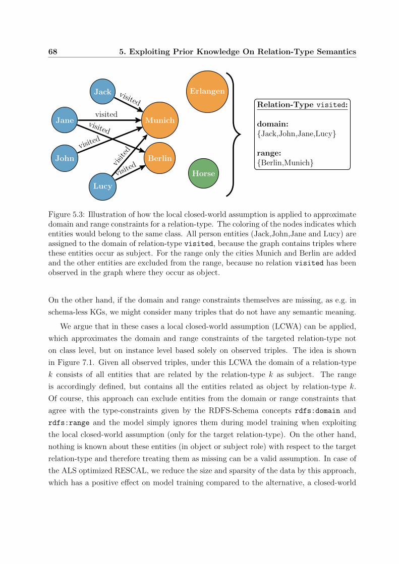
68 5. Exploiting Prior Knowledge On Relation-Type Semantics
Lucy
John
Jane
Jack
Berlin
Munich
Erlangen
Horsevisitedvi
sited
visited
visited
visited
visited Relation-Type visited:
domain:{Jack,John,Jane,Lucy}
range:{Berlin,Munich}
Figure 5.3: Illustration of how the local closed-world assumption is applied to approximatedomain and range constraints for a relation-type. The coloring of the nodes indicates whichentities would belong to the same class. All person entities (Jack,John,Jane and Lucy) areassigned to the domain of relation-type visited, because the graph contains triples wherethese entities occur as subject. For the range only the cities Munich and Berlin are addedand the other entities are excluded from the range, because no relation visited has beenobserved in the graph where they occur as object.
On the other hand, if the domain and range constraints themselves are missing, as e.g. in
schema-less KGs, we might consider many triples that do not have any semantic meaning.
We argue that in these cases a local closed-world assumption (LCWA) can be applied,
which approximates the domain and range constraints of the targeted relation-type not
on class level, but on instance level based solely on observed triples. The idea is shown
in Figure 7.1. Given all observed triples, under this LCWA the domain of a relation-type
k consists of all entities that are related by the relation-type k as subject. The range
is accordingly defined, but contains all the entities related as object by relation-type k.
Of course, this approach can exclude entities from the domain or range constraints that
agree with the type-constraints given by the RDFS-Schema concepts rdfs:domain and
rdfs:range and the model simply ignores them during model training when exploiting
the local closed-world assumption (only for the target relation-type). On the other hand,
nothing is known about these entities (in object or subject role) with respect to the target
relation-type and therefore treating them as missing can be a valid assumption. In case of
the ALS optimized RESCAL, we reduce the size and sparsity of the data by this approach,
which has a positive effect on model training compared to the alternative, a closed-world
5.3 A Local Closed-World Assumption for Modeling Knowledge Graphs 69
assumption that considers all entities to be part of the domain and range of the target
relation-type [56]. For the stochastic gradient descent optimized TransE and mwNN mod-
els, the corruption of triples will result in triples from which we can expect that they do
not disagree with the semantics of the corresponding relation-type.
5.3.1 Entity Grouping for RESCAL under a Local Closed-World
Assumption
In difference to the type-constraints, which were defined on entity class level, with the local
closed-world assumption we deliberately ignore the class membership of entities. As a con-
sequence, we loose the possibility to organize entities in large groups to reduce the amount
of inverses that have to be computed in the A-updates. We can reduce the amount of
different inverses by analyzing the data in a preprocessing step to group entities that share
the same pattern of inclusion in the approximated domain and range constraints through-
out all relation-types. Nevertheless, in large knowledge graphs where a large amount of
relation-types are present and completeness of entities will vary, the grouping will be less
successful, resulting in a large amount of small groups. Below, we will empirically study
the impact of the local closed-world assumption on the scalability of RESCAL using a large
knowledge graph extracted from DBpedia8 [66]. We extracted all entities with at least five
relations and all relation-types that have at least 1000 facts. The resulting graph contained
2,255,018 entities, 511 relation-types and 16,945,046 triples. The corresponding adjacency
tensor is of shape 2,255,018×2,255,018×511.
For evaluation and hyper-parameter-tuning we performed 10-fold cross-validation and
report the mean Area Under Precision Recall Curve (AUPRC) on a link prediction task.
We performed a similar 10-fold cross-validation procedure as used in Section 5.1.4 with the
DBpedia-Music data set, only in this case we defined the domain and range constraints
based on the local closed-world assumption 9. We also sampled 10 times as many negative
triples from the tensor and ran RESCAL with and without considering the local closed-
world assumption for 20 epochs of ALS. The experiment was conducted with an Intel(R)
Xeon(R) CPU W3520 @2.67GHz.
8http://wiki.dbpedia.org/Downloads39?v=pb8; Data set: Mapping-based Properties (Cleaned)9The domain and range constraints are expected to be not perfectly covering the type-constraints
defined by DBpedia’s schema, but will suffice to study the impact of the LCWA on RESCAL at this point
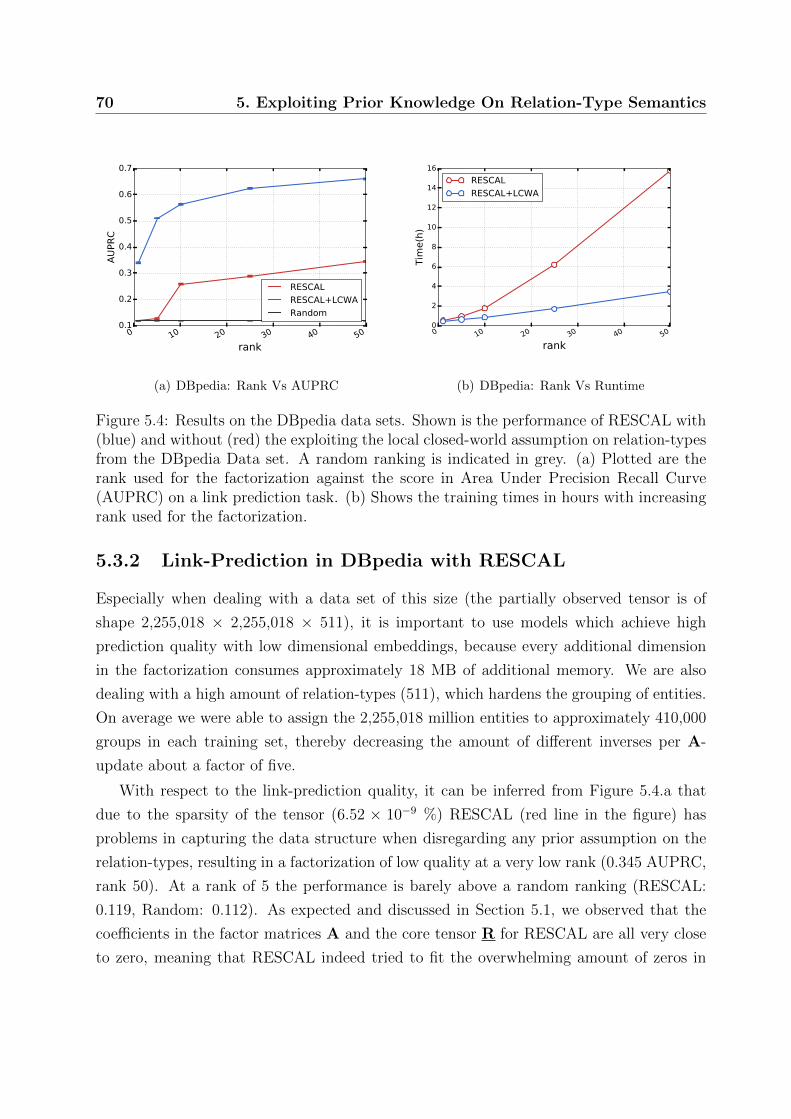
70 5. Exploiting Prior Knowledge On Relation-Type Semantics
0 10 20 30 40 50
rank
0.1
0.2
0.3
0.4
0.5
0.6
0.7
AUPRC
RESCAL
RESCAL+LCWA
Random
(a) DBpedia: Rank Vs AUPRC
0 10 20 30 40 50
rank
0
2
4
6
8
10
12
14
16
Time(h)
RESCAL
RESCAL+LCWA
(b) DBpedia: Rank Vs Runtime
Figure 5.4: Results on the DBpedia data sets. Shown is the performance of RESCAL with(blue) and without (red) the exploiting the local closed-world assumption on relation-typesfrom the DBpedia Data set. A random ranking is indicated in grey. (a) Plotted are therank used for the factorization against the score in Area Under Precision Recall Curve(AUPRC) on a link prediction task. (b) Shows the training times in hours with increasingrank used for the factorization.
5.3.2 Link-Prediction in DBpedia with RESCAL
Especially when dealing with a data set of this size (the partially observed tensor is of
shape 2,255,018 × 2,255,018 × 511), it is important to use models which achieve high
prediction quality with low dimensional embeddings, because every additional dimension
in the factorization consumes approximately 18 MB of additional memory. We are also
dealing with a high amount of relation-types (511), which hardens the grouping of entities.
On average we were able to assign the 2,255,018 million entities to approximately 410,000
groups in each training set, thereby decreasing the amount of different inverses per A-
update about a factor of five.
With respect to the link-prediction quality, it can be inferred from Figure 5.4.a that
due to the sparsity of the tensor (6.52 × 10⁻⁹ %) RESCAL (red line in the figure) has
problems in capturing the data structure when disregarding any prior assumption on the
relation-types, resulting in a factorization of low quality at a very low rank (0.345 AUPRC,
rank 50). At a rank of 5 the performance is barely above a random ranking (RESCAL:
0.119, Random: 0.112). As expected and discussed in Section 5.1, we observed that the
coefficients in the factor matrices A and the core tensor R for RESCAL are all very close
to zero, meaning that RESCAL indeed tried to fit the overwhelming amount of zeros in
5.3 A Local Closed-World Assumption for Modeling Knowledge Graphs 71
the data.
In comparison, by integrating approximated domain and range constraints (through
the local closed-world assumption), better factors that clearly capture structure in the
data could be learned at a rank of 5, resulting in an increased link-prediction quality of
0.511 in AUPRC (RESCAL+LCWA, blue line in Figure 5.4.a). Furthermore, at a rank of
50 the factorization starts to become of reasonable quality (0.667)10 whereas the original
algorithm clearly fails (0.345). It can be expected that the original RESCAL will actually
achieve similar results when exploiting a sufficiently high rank but, as discussed in Chapter
4, for very large data sets a high rank is intractable or at least a powerful computer system
needed.
In Figure 5.4.b, we show the runtime of both RESCAL approaches after 20 epochs of
ALS. It can be clearly seen that the training time differences are significantly diverging
with higher ranks and the consideration of the approximated domain and range constraints
clearly decreases RESCAL’s training time. By exploiting the LCWA, the data can be fac-
torized with a rank of 50 in about 3.5 hours (RESCAL+LCWA, AUPRC: 0.667) whereas
the original algorithm needs almost 16 hours (RESCAL, AUPRC: 0.345). On a multi-
relational data set of this size, where relation-types incorporate only a small subset of
entities, the calculations in the updates based on the much smaller factor matrices be-
come very efficient and the larger amount of inverse computations per A-update become
insignificant. With increasing rank the gap in training time is expected to increase even
further.
5.3.3 Conclusion
Type-constraints of relation-types from schema-based knowledge graphs are not neces-
sarily always present or can be fuzzy. We proposed an alternative local closed-world
assumption that can be applied in these cases. This local closed-world assumption ap-
proximates domain and range constraints solely based on observed triples in the graph.
In case of RESCAL, the approximated domain and range constraints do not consider the
class membership of entities and therefore the grouping of entities, which is exploited for
decreasing the amount of inverse computations in the A-updates (Section 5.1.2), is less
efficient. Based on our experiments on a very large sample from the DBpedia knowledge
graph, we were able to show that this drawback is negligible. In fact, we could observe
that the local closed-world assumption adds great value to RESCAL, improving runtime
10The corresponding Area under ROC curve is 0.84.
72 5. Exploiting Prior Knowledge On Relation-Type Semantics
and link-prediction quality significantly by exploiting low-dimensional embeddings at the
same time.
5.4 Experiments – Prior Knowledge on Relation-Types
is Important for Latent Variable Models
In the previous sections, we have shown how prior knowledge about relation-types can be
integrated in ALS optimized RESCAL and SGD optimized TransE and mwNN. We showed
that in case of RESCAL, domain and range constraints as given by the schema of the
knowledge graph or derived by a local closed-world assumption increase the link-prediction
quality significantly, if integrated into the optimization algorithm. In this section, we want
to study the general value of prior knowledge on the semantics of relation-types for the
statistical modeling of knowledge graphs with latent variable models. In the first setting,
we assume that curated type-constraints extracted from the knowledge graph’s schema are
available. In the second setting, we explore the local closed-world assumption proposed
in Section 5.3. Our experimental setup covers three important aspects which will enable
us to make generalizing conclusions about the importance of such prior knowledge when
applying latent variable models to large knowledge graphs:
• We test various representative latent variable models that cover the diversity of these
models in the domain. As motivated in the introduction of Chapter 3.3, we belief
that RESCAL, TransE and mwNN are especially well suited for this task.
• We test these models at reasonable low complexity levels, meaning that we enforce
low dimensional latent embeddings, which simulates their application to very large
data sets where high dimensional embeddings are intractable. In [25] for example,
the dimensionality of the latent embeddings (d in Chapter 3.3.4) was chosen to be
60.
• We extracted diverse data sets from instances of the Linked-Open Data Cloud,
namely Freebase, YAGO and DBpedia, because it is expected that the value of prior
knowledge about relation-type semantics is also dependent on the particular data
set the models are applied to. From these knowledge graphs, we constructed data
sets that will be used as representatives for general purpose knowledge graphs that
cover a wide range of relation-types from a diverse set of domains, domain focused
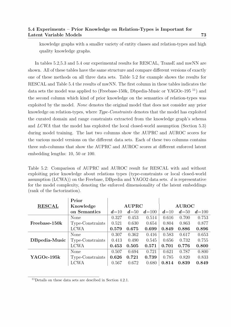
5.4 Experiments – Prior Knowledge on Relation-Types is Important forLatent Variable Models 73
knowledge graphs with a smaller variety of entity classes and relation-types and high
quality knowledge graphs.
In tables 5.2,5.3 and 5.4 our experimental results for RESCAL, TransE and mwNN are
shown. All of these tables have the same structure and compare different versions of exactly
one of these methods on all three data sets. Table 5.2 for example shows the results for
RESCAL and Table 5.4 the results of mwNN. The first column in these tables indicates the
data sets the model was applied to (Freebase-150k, Dbpedia-Music or YAGOc-195 11) and
the second column which kind of prior knowledge on the semantics of relation-types was
exploited by the model. None denotes the original model that does not consider any prior
knowledge on relation-types, where Type-Constraints denotes that the model has exploited
the curated domain and range constraints extracted from the knowledge graph’s schema
and LCWA that the model has exploited the local closed-world assumption (Section 5.3)
during model training. The last two columns show the AUPRC and AUROC scores for
the various model versions on the different data sets. Each of these two columns contains
three sub-columns that show the AUPRC and AUROC scores at different enforced latent
embedding lengths: 10, 50 or 100.
Table 5.2: Comparison of AUPRC and AUROC result for RESCAL with and withoutexploiting prior knowledge about relations types (type-constraints or local closed-worldassumption (LCWA)) on the Freebase, DBpedia and YAGO2 data sets. d is representativefor the model complexity, denoting the enforced dimensionality of the latent embeddings(rank of the factorization).
PriorKnowledgeon Semantics
AUPRC AUROCRESCALd=10 d=50 d=100 d=10 d=50 d=100
Freebase-150kNone 0.327 0.453 0.514 0.616 0.700 0.753Type-Constraints 0.521 0.630 0.654 0.804 0.863 0.877LCWA 0.579 0.675 0.699 0.849 0.886 0.896
DBpedia-MusicNone 0.307 0.362 0.416 0.583 0.617 0.653Type-Constraints 0.413 0.490 0.545 0.656 0.732 0.755LCWA 0.453 0.505 0.571 0.701 0.776 0.800
YAGOc-195kNone 0.507 0.694 0.721 0.621 0.787 0.800Type-Constraints 0.626 0.721 0.739 0.785 0.820 0.833LCWA 0.567 0.672 0.680 0.814 0.839 0.849
11Details on these data sets are descibed in Section 4.2.1.
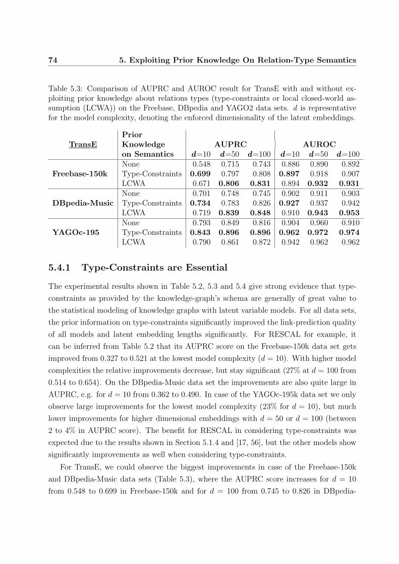
74 5. Exploiting Prior Knowledge On Relation-Type Semantics
Table 5.3: Comparison of AUPRC and AUROC result for TransE with and without ex-ploiting prior knowledge about relations types (type-constraints or local closed-world as-sumption (LCWA)) on the Freebase, DBpedia and YAGO2 data sets. d is representativefor the model complexity, denoting the enforced dimensionality of the latent embeddings.
PriorKnowledgeon Semantics
AUPRC AUROCTransEd=10 d=50 d=100 d=10 d=50 d=100
Freebase-150kNone 0.548 0.715 0.743 0.886 0.890 0.892Type-Constraints 0.699 0.797 0.808 0.897 0.918 0.907LCWA 0.671 0.806 0.831 0.894 0.932 0.931
DBpedia-MusicNone 0.701 0.748 0.745 0.902 0.911 0.903Type-Constraints 0.734 0.783 0.826 0.927 0.937 0.942LCWA 0.719 0.839 0.848 0.910 0.943 0.953
YAGOc-195None 0.793 0.849 0.816 0.904 0.960 0.910Type-Constraints 0.843 0.896 0.896 0.962 0.972 0.974LCWA 0.790 0.861 0.872 0.942 0.962 0.962
5.4.1 Type-Constraints are Essential
The experimental results shown in Table 5.2, 5.3 and 5.4 give strong evidence that type-
constraints as provided by the knowledge-graph’s schema are generally of great value to
the statistical modeling of knowledge graphs with latent variable models. For all data sets,
the prior information on type-constraints significantly improved the link-prediction quality
of all models and latent embedding lengths significantly. For RESCAL for example, it
can be inferred from Table 5.2 that its AUPRC score on the Freebase-150k data set gets
improved from 0.327 to 0.521 at the lowest model complexity (d = 10). With higher model
complexities the relative improvements decrease, but stay significant (27% at d = 100 from
0.514 to 0.654). On the DBpedia-Music data set the improvements are also quite large in
AUPRC, e.g. for d = 10 from 0.362 to 0.490. In case of the YAGOc-195k data set we only
observe large improvements for the lowest model complexity (23% for d = 10), but much
lower improvements for higher dimensional embeddings with d = 50 or d = 100 (between
2 to 4% in AUPRC score). The benefit for RESCAL in considering type-constraints was
expected due to the results shown in Section 5.1.4 and [17, 56], but the other models show
significantly improvements as well when considering type-constraints.
For TransE, we could observe the biggest improvements in case of the Freebase-150k
and DBpedia-Music data sets (Table 5.3), where the AUPRC score increases for d = 10
from 0.548 to 0.699 in Freebase-150k and for d = 100 from 0.745 to 0.826 in DBpedia-
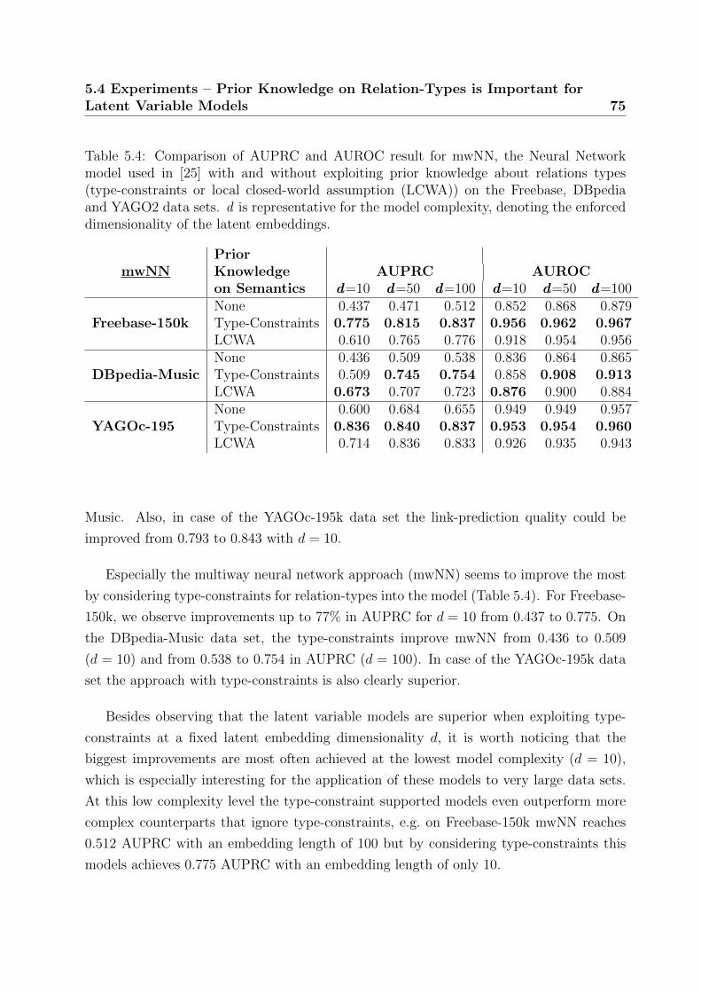
5.4 Experiments – Prior Knowledge on Relation-Types is Important forLatent Variable Models 75
Table 5.4: Comparison of AUPRC and AUROC result for mwNN, the Neural Networkmodel used in [25] with and without exploiting prior knowledge about relations types(type-constraints or local closed-world assumption (LCWA)) on the Freebase, DBpediaand YAGO2 data sets. d is representative for the model complexity, denoting the enforceddimensionality of the latent embeddings.
PriorKnowledgeon Semantics
AUPRC AUROCmwNNd=10 d=50 d=100 d=10 d=50 d=100
Freebase-150kNone 0.437 0.471 0.512 0.852 0.868 0.879Type-Constraints 0.775 0.815 0.837 0.956 0.962 0.967LCWA 0.610 0.765 0.776 0.918 0.954 0.956
DBpedia-MusicNone 0.436 0.509 0.538 0.836 0.864 0.865Type-Constraints 0.509 0.745 0.754 0.858 0.908 0.913LCWA 0.673 0.707 0.723 0.876 0.900 0.884
YAGOc-195None 0.600 0.684 0.655 0.949 0.949 0.957Type-Constraints 0.836 0.840 0.837 0.953 0.954 0.960LCWA 0.714 0.836 0.833 0.926 0.935 0.943
Music. Also, in case of the YAGOc-195k data set the link-prediction quality could be
improved from 0.793 to 0.843 with d = 10.
Especially the multiway neural network approach (mwNN) seems to improve the most
by considering type-constraints for relation-types into the model (Table 5.4). For Freebase-
150k, we observe improvements up to 77% in AUPRC for d = 10 from 0.437 to 0.775. On
the DBpedia-Music data set, the type-constraints improve mwNN from 0.436 to 0.509
(d = 10) and from 0.538 to 0.754 in AUPRC (d = 100). In case of the YAGOc-195k data
set the approach with type-constraints is also clearly superior.
Besides observing that the latent variable models are superior when exploiting type-
constraints at a fixed latent embedding dimensionality d, it is worth noticing that the
biggest improvements are most often achieved at the lowest model complexity (d = 10),
which is especially interesting for the application of these models to very large data sets.
At this low complexity level the type-constraint supported models even outperform more
complex counterparts that ignore type-constraints, e.g. on Freebase-150k mwNN reaches
0.512 AUPRC with an embedding length of 100 but by considering type-constraints this
models achieves 0.775 AUPRC with an embedding length of only 10.
76 5. Exploiting Prior Knowledge On Relation-Type Semantics
5.4.2 Local Closed-World Assumption – Simple but Powerful
In Section 5.4.1 we have declared based on empirical results that type-constraints are very
important for the statistical modeling of knowledge graphs with latent-variable models.
Unfortunately, type-constraints are not always available or can be fuzzy for some relation-
types due to incompleteness of the underlying knowledge graph. The local closed-world
assumption (LCWA) discussed in Section 5.3 offers an alternative in these cases because
it relies solely on observed triples.
It can be observed from tables 5.2, 5.3 and 5.4 that similar to the type-constraints, the
approximation of domain and range constraints through the Local Closed-World Assump-
tion generally leads to large improvements in link prediction results over the same models
that do not consider any prior knowledge about relation-types, especially at the lowest
model complexities (d = 10). For example, TransE gets improved from 0.715 to 0.806 with
d = 50 in the Freebase-150k data set, mwNN improves its initial AUPRC score of 0.600
(d = 10) on the YAGO data set to 0.714 and RESCAL’s AUPRC score jumps from 0.327
to 0.579 (d = 10). The only exception to these observation is RESCAL when applied to
the YAGOc-195k data set. For d = 50, RESCAL’s AUPRC score decreases from 0.694 to
0.672 and for d = 100 from 0.721 to 0.680 when considering the LCWA in the model. The
type-constraints of the relation-types in the YAGOc-195 data set are defined over a large
set of entities (we evaluate on the type-constrained knowledge graph). When applying
type-constraints to the YAGOc-195k data set, 22% of all possible triples are covered. It
seems that a closed-world assumption is more beneficial for RESCAL than a LCWA in this
case.
Even though the LCWA has a similar strong impact on link-prediction quality than
the curated type-constraints, there is no evidence in our experiments that the LCWA can
generally replace the semantic prior knowledge about entity types and type-constraints on
relation-types given by the schema of the knowledge-graph. For the YAGOc-195k data
set the AUPRC scores for the models that exploit the LCWA are often clearly worse
than their counterparts that use the type-constraints extracted from the knowledge graph.
TransE with type-constraints achieves an AUPRC score of 0.896 whereas LCWA supported
TransE reaches only 0.861 with an embedding length of 50. For d = 10, mwNN with type-
constraints reaches an AUPRC score 0.836 whereas the application of the LCWA leads
only to 0.714.
In case of the other two data sets the message is not as clear. RESCAL achieves its
best results when exploiting LCWA instead of type-constraints, whereas TransE shows
5.5 Related Work 77
better performance only for latent embeddings of length 50 and 100 but not with a length
of 10. For d = 100, the combination of TransE and the LCWA improves the AUPRC
score to 0.831 (0.808 with type-constraints) in Freebase-150k and 0.839 (0.783 with type-
constraints) in DBpedia-Music. At the lowest model complexity (d = 10) on the other
hand, the integration of type-constraints is superior over the LCWA.
For mwNN the observations are the opposite to those of the TransE extensions in case
of DBpedia-Music. In case of the Freebase-150k data set the integration of the extracted
type-constraints is always clearly better, reaching 0.815 in AUPRC with an embedding
length of 10 (0.765 with LCWA).
5.5 Related Work
A general overview on the related work in the field of statistical modeling of knowledge
graphs with latent variable models is provided in Chapter 4.4. Integrating domain and
range constraints as given by the knowledge graph’s schema into RESCAL has also been
proposed by [17]. Local closed-world assumptions are a known concept in the semantic
web domain [96]. The neural network approach used in the Google Knowledge Vault
System, in this work denoted as mwNN, also exploits a local closed-world assumption for
corrupting triples (negative sampling). As described in Chapter 3.3.4, this local closed-
world assumption only excludes unobserved subject entities from the negative sampling.
In difference to the local closed-world assumption used in this chapter, the object entity of
an observed triple can be corrupted through any entity present in the knowledge graph.
In case of RESCAL, prior information on type-constraints can also be integrated by
the method proposed in [69], which introduced a weighted loss functions for RESCAL. Via
such loss functions relational type-constraints are integrated in the RESCAL optimization
by assigning zero weights to triples that are excluded through type-constraints. Unfortu-
nately, the scalability of RESCAL gets lost when using this type of weighted loss function.
The Hadamard (element wise) matrix product with the weighting tensor leads to expen-
sive matrix operations in the gradients, since a materialization of a complete frontal slice
reconstructed from the learned latent representation of the data is required (the product
ARkAT ), which is dense. Besides the high computational costs that arise during this ma-
terialization in the gradient, the memory requirements for this materialization itself will
be extensive which makes this approach impractical for large knowledge graphs. For ex-
ample, consider the music domain of DBPedia (321,950 entities). The materialization of
78 5. Exploiting Prior Knowledge On Relation-Type Semantics
a single frontal slice (ARkAT ) will need approximately 829 GB of memory (considering
double precision floats).
5.6 Conclusion
In this chapter, we have motivated and studied the general value of prior knowledge about
the semantics of relation-types extracted from the schema of the knowledge-graph (type-
constraints) or approximated through a local closed-world assumption for the statistical
modeling of knowledge graphs with latent variable models. We have shown that this
prior knowledge can be integrated in the ALS optimized RESCAL, but also in the SGD
optimized TransE and mwNN models without sacrificing the scalability of these models.
Our experiments give clear empirical proof that the curated semantic information of type-
constraints significantly improves link-prediction quality of TransE, RESCAL and mwNN
(up to 77%) and can therefore be considered as essential for latent variable models when
applied to large knowledge graphs. In this regard, the value of type-constraints becomes
especially prominent when the model complexity, i.e. the dimensionality of the embeddings,
has to be very low which is an essential requirement when applying these models to very
large data sets.
Since type-constraints are not always present or can be fuzzy (due to e.g. insufficient
typing of entities) we further showed that an alternative, a local closed-world assumption
(LCWA), can be applied in these cases that approximates domain and range constraints on
instance rather on class level solely based on observed triples. This LCWA leads to similar
large improvements in the link-prediction tasks than the type-constraints, but especially
at a very low model complexity the integration of type-constraints seemed superior. In our
experiments we used models that either exploited type-constraints or the LCWA, but in
a real setting we would combine both, where type-constraints are used whenever possible
and the LCWA in case type-constraints are absent or fuzzy.
Chapter 6Ensemble Solutions for Representation
Learning in Knowledge Graphs
We have motivated in Chapter 3.3 that RESCAL[82], TransE [9] and the multiway neural
network proposed in [25] (mwNN) represent the diversity of state of the art latent vari-
able models for the statistical modeling of knowledge graphs. In the last chapter, we have
shown that these models can be improved individually by integrating prior knowledge
about relation-types in form of type-constraints or derived through a local closed-world
assumption. In this regard and in Chapter 4.3, we could observe that these models also
differ in their link-prediction capabilities when applied to large knowledge graphs under
realistic settings. A large amount of literature is putting a lot of effort in finding the
best model for a certain use-case in the context of knowledge graphs, e.g. link-prediction,
selling the proposed method as the superior overall model. From our opinion, it is often
disregarded that these models might model different aspects of the data and therefore even
models with lower prediction quality are able to contribute non redundant dependencies
learned from the data. In all of our experiments, TransE often significantly outperformed
the other two methods on the tested data sets in link-prediction tasks, but we argue that
all three methods are substantially different in multiply aspects regarding their modeling
assumptions and technical details and therefore chances are high that they learn different
patterns in the data that can be complemented. In this chapter, we study the comple-
mentary potential of these models by combining them in very simple ensembles. We also
consider type-constraints and the local closed-world assumption in the individual models,
due to their importance for the statistical modeling of knowledge graphs (see Chapter 5).
Based on the conducted experiments on multiple datasets, we show that TransE’s link
80 6. Ensemble Solutions for Representation Learning in Knowledge Graphs
predictions are complemented by predictions made by RESCAL and mwNN.
The content of this chapter is completely covered in:
[58] Denis Krompaß and Volker Tresp. Ensemble Solutions for Representation Learning
in Knowledge Graphs ECML Workshop on Linked Data for Knowledge Discovery.
2015
6.1 Studying Complementary Effects between TransE,
RESCAL and mwNN
The main characteristic of a good ensemble is its composition out of very diverse single
predictors that learn and recognize different patterns in the data. Through the diversity
of the different predictors often complementary effects can be observed that drive overall
prediction quality. As discussed in chapter 3.3, there is a large diversity between RESCAL,
TransE and mwNN. RESCAL assumes normally distributed variables minimizing a least-
squares loss function, whereas mwNN assumes Bernoulli distributed variables minimizing
a logistic loss function. TransE on the other hand minimizes a max-margin based ranking
loss function. Furthermore, RESCAL is a third-order tensor factorization method that
is optimized through alternating least-squares, whereas TransE is a distance based model
and mwNN a neural network that are both optimized through stochastic gradient-descent
combined with negative sampling. In addition, mwNN and TransE differ in the way they
corrupt triples for the negative sampling. In TransE, two corrupted triples are sampled for
each true triple, where in each corrupted triple the subject or object entity is replaced (but
never at the same time). mwNN generates negative triples by only corrupting the object
entities with randomly sampled entities. In difference to the other methods, TransE does
not include any regularization besides enforcing an L2-norm of 1 for the latent embeddings
of the entities. RESCAL uses a L2 regularization and we minimized mwNN with elastic
net regularization and additional DropConnect [111] on the network weights.
For our study, we build simple ensembles in which we combine the link-predictions of
RESCAL, TransE and mwNN. The final probability of a triple is then derived from the
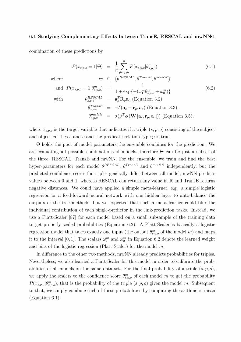
6.1 Studying Complementary Effects between TransE, RESCAL and mwNN81
combination of these predictions by
P (xs,p,o = 1|Θ) =1
n
n∑θm∈Θ
P (xs,p,o|θms,p,o) (6.1)
where Θ ⊆ {θRESCAL, θTransE, θmwNN}
and P (xs,p,o = 1|θms,p,o) =1
1 + exp{−(ωm1 θms,p,o + ωm0 )}
(6.2)
with θRESCALs,p,o = aTs Rpao (Equation 3.2),
θTransEs,p,o = −δ(as + rp, ao) (Equation 3.3),
θmwNNs,p,o = σ(βTφ (W [as, rp, ao])) (Equation 3.5),
where xs,p,o is the target variable that indicates if a triple (s, p, o) consisting of the subject
and object entities s and o and the predicate relation-type p is true.
Θ holds the pool of model parameters the ensemble combines for the prediction. We
are evaluating all possible combinations of models, therefore Θ can be just a subset of
the three, RESCAL, TransE and mwNN. For the ensemble, we train and find the best
hyper-parameters for each model θRESCAL, θTransE and θmwNN independently, but the
predicted confidence scores for triples generally differ between all model; mwNN predicts
values between 0 and 1, whereas RESCAL can return any value in R and TransE returns
negative distances. We could have applied a simple meta-learner, e.g. a simple logistic
regression or a feed-forward neural network with one hidden layer to auto-balance the
outputs of the tree methods, but we expected that such a meta learner could blur the
individual contribution of each single-predictor in the link-prediction tasks. Instead, we
use a Platt-Scaler [87] for each model based on a small subsample of the training data
to get properly scaled probabilities (Equation 6.2). A Platt-Scaler is basically a logistic
regression model that takes exactly one input (the output θms,p,o of the model m) and maps
it to the interval [0, 1]. The scalars ωm1 and ωm0 in Equation 6.2 denote the learned weight
and bias of the logistic regression (Platt-Scaler) for the model m.
In difference to the other two methods, mwNN already predicts probabilities for triples.
Nevertheless, we also learned a Platt-Scaler for this model in order to calibrate the prob-
abilities of all models on the same data set. For the final probability of a triple (s, p, o),
we apply the scalers to the confidence score θms,p,o of each model m to get the probability
P (xs,p,o|θms,p,o), that is the probability of the triple (s, p, o) given the model m. Subsequent
to that, we simply combine each of these probabilities by computing the arithmetic mean
(Equation 6.1).
82 6. Ensemble Solutions for Representation Learning in Knowledge Graphs
6.2 Experimental Setup
With our experiments we study if TransE, RESCAL and mwNN are good targets for
combination to drive link-prediction quality. We will further check if one model is not
contributing any additional knowledge to the ensemble by evaluating ensembles where
only two of the three models are combined. The above two steps are evaluated in two
settings, where in the first setting the models are exploiting type-constraints extracted
from the knowledge-base schema and in the second setting they solely use the local closed-
world assumption (LCWA) proposed in Chapter 5.3. With the second setting we check
if LCWA based models are also learning complementary information. As discussed in
chapter 5.3 the LCWA has the benefit that it can be exploited without the need of prior
knowledge about the types of the entities and the typing of the relation-types. Therefore
they can be applied to single relation-types or whole knowledge-graphs where information
about type-constraints is absent or fuzzy. We evaluate the different ensembles on link-
prediction tasks, using the same data sets (Freebase-150k, Dbpedia-Music, YAGOc-195k)
and evaluation procedure as described in Chapter 4.2.1 and 4.2.2. The ensembles were also
implemented in python using the code of RESCAL, TransE and mwNN, which has been
described in Chapter 4.2.3. After hyper-parameter tuning we retrained all models using
the best hyper-parameters on the validation and training set and used 5% of this combined
training set for learning the Platt-Scalers for each model (RESCAL, TransE and mwNN).
We report the Area Under Precision Recall Curve (AUPRC) score for each ensemble and
in addition we report the AUPRC for the best single predictor as comparison.
6.3 Experiments – TransE, RESCAL and mwNN Learn
Complementary Aspects in Knowledge Graphs
In Table 6.1 the AUPRC results on the extracted data sets from Freebase, YAGO and
DBpedia for the first setting are shown, where all models exploit the type-constraints given
by the RDF-Schema concepts. Table 6.2 shows the same for the second setting where the
models solely exploited the Local Closed-World Assumption. ALL represents the ensemble
consisting of TransE, RESCAL and mwNN and the beneath three models represent the
ensembles that combine all possible pairs of models, e.g. mwNN + TransE represents the
ensemble consisting of mwNN and TransE. Best Single Predictor represents the best model
out of TransE, RESCAL or mwNN on the same link-prediction task. Which of the three
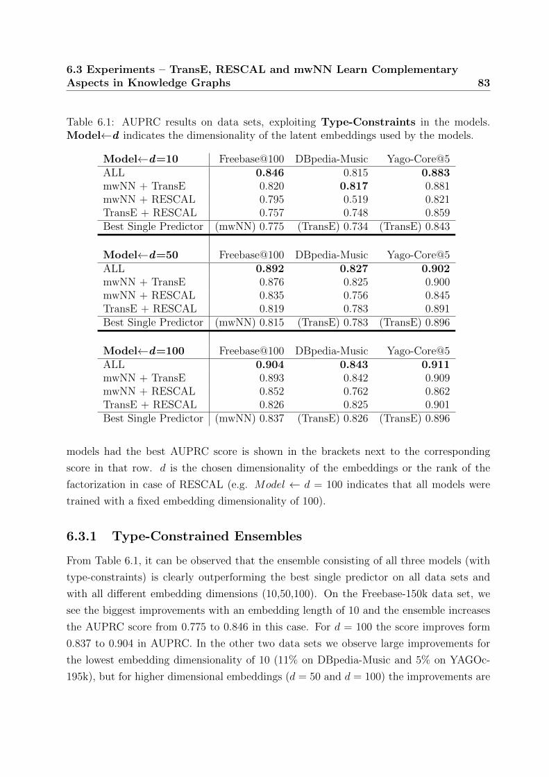
6.3 Experiments – TransE, RESCAL and mwNN Learn ComplementaryAspects in Knowledge Graphs 83
Table 6.1: AUPRC results on data sets, exploiting Type-Constraints in the models.Model←d indicates the dimensionality of the latent embeddings used by the models.
Model←d=10 Freebase@100 DBpedia-Music Yago-Core@5ALL 0.846 0.815 0.883mwNN + TransE 0.820 0.817 0.881mwNN + RESCAL 0.795 0.519 0.821TransE + RESCAL 0.757 0.748 0.859Best Single Predictor (mwNN) 0.775 (TransE) 0.734 (TransE) 0.843
Model←d=50 Freebase@100 DBpedia-Music Yago-Core@5ALL 0.892 0.827 0.902mwNN + TransE 0.876 0.825 0.900mwNN + RESCAL 0.835 0.756 0.845TransE + RESCAL 0.819 0.783 0.891Best Single Predictor (mwNN) 0.815 (TransE) 0.783 (TransE) 0.896
Model←d=100 Freebase@100 DBpedia-Music Yago-Core@5ALL 0.904 0.843 0.911mwNN + TransE 0.893 0.842 0.909mwNN + RESCAL 0.852 0.762 0.862TransE + RESCAL 0.826 0.825 0.901Best Single Predictor (mwNN) 0.837 (TransE) 0.826 (TransE) 0.896
models had the best AUPRC score is shown in the brackets next to the corresponding
score in that row. d is the chosen dimensionality of the embeddings or the rank of the
factorization in case of RESCAL (e.g. Model ← d = 100 indicates that all models were
trained with a fixed embedding dimensionality of 100).
6.3.1 Type-Constrained Ensembles
From Table 6.1, it can be observed that the ensemble consisting of all three models (with
type-constraints) is clearly outperforming the best single predictor on all data sets and
with all different embedding dimensions (10,50,100). On the Freebase-150k data set, we
see the biggest improvements with an embedding length of 10 and the ensemble increases
the AUPRC score from 0.775 to 0.846 in this case. For d = 100 the score improves form
0.837 to 0.904 in AUPRC. In the other two data sets we observe large improvements for
the lowest embedding dimensionality of 10 (11% on DBpedia-Music and 5% on YAGOc-
195k), but for higher dimensional embeddings (d = 50 and d = 100) the improvements are
84 6. Ensemble Solutions for Representation Learning in Knowledge Graphs
decreasing or vanishing (YAGOc-195k).
The improvements observed for the really low embedding vector dimensionality of 10
are of special interest. As discussed in Chapter 4, in a Web-Scale application of these
algorithms it is of high interest to have meaningful embeddings in a very low dimensional
latent space because higher dimensional representations can lead to long or even intractable
runtimes for model training and tuning. It can be observed that the ensemble consisting
of TransE, RESCAL and mwNN with a embedding length of 10 reaches comparable link
prediction results than the best single predictor with an embedding vector length of 100.
On the Freebase-150k data set the ensemble reaches an AUPRC score of 0.846, on DBpedia-
Music 0.815 and YAGOc-195k 0.883 with d = 10, whereas the best single predictor reaches
0.837, 0.826 and 0.896, respectively, with d = 100.
When it comes to the contribution of each single predictor to the ensemble, we observe
that in case of the Freebase data set all models are contributing to the superior perfor-
mance of the ensemble, but TransE and mwNN are responsible for the biggest increase in
AUPRC. For example, with d = 10 TransE+mwNN achieves an AUPRC of 0.820 whereas
mwNN+RESCAL reaches 0.795 and TransE+RESCAl 0.757. On the DBpedia-Music and
YAGOc-195k data set, RESCAL does not add any significant value to the ensemble, e.g.
for d = 50 mwNN+TransE have the highest AUPRC score of the pairwise ensembles reach-
ing already 0.825 on DBpedia-Music and 0.900 on YAGOc-195k, whereas the maximum
performance of the complete ensemble (ALL) lies at 0.827 and 0.902.
As a final remark we could observe from the results shown in Table 6.1 that RESCAL or
mwNN best complement with TransE. The combination of mwNN and RESCAL generally
shows less improvements in AUPRC compared to the best single predictor performance of
those two (compare with Tables 5.2, 5.3 and 5.4), indicating that these two models learn
more similar patterns from the data.
6.3.2 Ensembles under a Local Closed-World Assumption
The results for the LCWA ensemble are shown in Table 6.2. We see the largest improve-
ments on the Freebase-150k data set, where the ensemble improves the AUPRC score
compared to the best single predictor from 15% (d = 10) to 9% (d = 100). Also, all predic-
tors (RESCAL,TransE, mwNN) contribute to the performance of the ensemble, since all
ensembles consisting of two models achieve a significantly lower AUPRC score in this case.
The highest pair-ensemble (TransE + RESCAL) achieves 0.763 (d = 10), 0.876 (d = 50)
and 0.899 (d = 100) whereas the full ensemble achieves 0.775, 0.886 and 0.909. On the
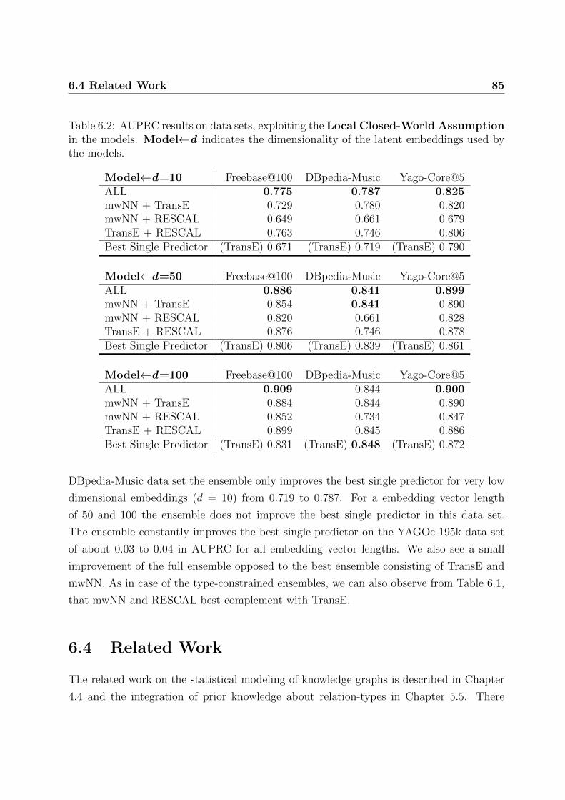
6.4 Related Work 85
Table 6.2: AUPRC results on data sets, exploiting the Local Closed-World Assumptionin the models. Model←d indicates the dimensionality of the latent embeddings used bythe models.
Model←d=10 Freebase@100 DBpedia-Music Yago-Core@5ALL 0.775 0.787 0.825mwNN + TransE 0.729 0.780 0.820mwNN + RESCAL 0.649 0.661 0.679TransE + RESCAL 0.763 0.746 0.806Best Single Predictor (TransE) 0.671 (TransE) 0.719 (TransE) 0.790
Model←d=50 Freebase@100 DBpedia-Music Yago-Core@5ALL 0.886 0.841 0.899mwNN + TransE 0.854 0.841 0.890mwNN + RESCAL 0.820 0.661 0.828TransE + RESCAL 0.876 0.746 0.878Best Single Predictor (TransE) 0.806 (TransE) 0.839 (TransE) 0.861
Model←d=100 Freebase@100 DBpedia-Music Yago-Core@5ALL 0.909 0.844 0.900mwNN + TransE 0.884 0.844 0.890mwNN + RESCAL 0.852 0.734 0.847TransE + RESCAL 0.899 0.845 0.886Best Single Predictor (TransE) 0.831 (TransE) 0.848 (TransE) 0.872
DBpedia-Music data set the ensemble only improves the best single predictor for very low
dimensional embeddings (d = 10) from 0.719 to 0.787. For a embedding vector length
of 50 and 100 the ensemble does not improve the best single predictor in this data set.
The ensemble constantly improves the best single-predictor on the YAGOc-195k data set
of about 0.03 to 0.04 in AUPRC for all embedding vector lengths. We also see a small
improvement of the full ensemble opposed to the best ensemble consisting of TransE and
mwNN. As in case of the type-constrained ensembles, we can also observe from Table 6.1,
that mwNN and RESCAL best complement with TransE.
6.4 Related Work
The related work on the statistical modeling of knowledge graphs is described in Chapter
4.4 and the integration of prior knowledge about relation-types in Chapter 5.5. There
86 6. Ensemble Solutions for Representation Learning in Knowledge Graphs
has been little amount of work on combining latent variable models for link-prediction
in knowledge graphs. Very recently, [36] combined two independent models of different
complexity in an ensemble (TATEC) to improve link-prediction. As in [99] a three-way
model is combined with a two-way model in this case, but in TATEC the two models
are trained independently and combined later. [43] used a bagging approach to combine
various classification algorithms (e.g. Support-Vector-Machines, K-Nearest-Neighbor) for
link-prediction, but could not observe any significant improvements over the best single
predictors.
6.5 Conclusion
In this work we showed that the the predictions of three leading latent variable models for
link-prediction in large knowledge-graphs are indeed complementary to each other and can
be exploited in an ensemble solution to improve overall link-prediction quality. We observed
in our experiments that especially TransE learns substantially different aspects of the data
than RESCAL and mwNN. RESCAL and mwNN on the other hand are more similar to
each other, even though these two models differ in various aspects. We further showed
that an ensemble consisting of all three methods brings substantially higher prediction
quality on all used data sets and all settings when the models need to exploit a very low
dimensional embedding space (d = 10). The LCWA can also be exploited in the ensemble
when the type-constraints for properties are absent or fuzzy. On the DBpedia-Music and
YAGOc-195 data set we observed that with a higher dimensional latent embedding space
the improvements become less significant.
Chapter 7Querying Statistically Modeled Knowledge
Graphs
It is a known fact that the Web of Data is fairly incomplete and contains incorrect infor-
mation, as triples are missing and existing triples can be false. Generally, information in
the form of triples extracted from such data is afflicted with uncertainty that is persis-
tent in the source data, has been introduced by human curators or information extraction
methods. In many cases, the valuable information about uncertainty is discarded and some
threshold is applied to filter more probable triples, which is dependent on the extraction
technique applied. When accessing these data sets, we typically only see what is left after
this pruning step and the information about the uncertainties is irreparably lost.
In the previous chapters, we have shown that latent variable models are powerful mod-
els that are especially well suited for the statistical modeling of knowledge graphs and that
generate confidence values for observed and unobserved triples which can be exploited for
the completion and cleansing of knowledge graphs. In other words, these models reintro-
duce a measure of uncertainty into the graph that represents the beliefs of the model into
observed and unobserved triples derived from the learned dependencies in the data. Ap-
plying latent variable models for link-prediction tasks can be seen as querying these models
for ground triples to derive probabilities that describe the likelihood of their occurrences
over the vast amount of possible deterministic instantiations (worlds) of the graph. Prob-
abilistic databases (PDBs) naturally consider multiple possible instances of a database via
the possible worlds semantics and account for uncertainty in the data by assigning a prob-
ability distribution over all of these database instances [100]. As a conclusion, we could
interpret the statistically modeled knowledge graph as a probabilistic database, where the
88 7. Querying Statistically Modeled Knowledge Graphs
latent variable model is defining the underlying probability distribution of triples. As such,
we could proceed and exploit these modeled graphs for complex querying that goes beyond
the querying of ground triples. Querying probabilistic databases has a clear interpretation
as generalization of deterministic relational database querying.
When applying PDBs to large triple stores, various key challenges need to be addressed.
First, we have to consider storage requirements. A common assumption in PDBs is tuple
independence, or in our case triple independence, which requires a representation of each
triple’s uncertainty. Unless default values are used, representing the individual uncertainty
levels can lead to huge storage requirements.
Second, probabilistically correct and efficient querying. Although individual triples
are assumed to be independent, complex queries introduce dependencies such that correct
query answering becomes, in the worst case, intractable.
These two challenges are intertwined, since we cannot explicitly represent the uncer-
tainty values of all possible triples, and the generation of these uncertainties “on the fly”
during query evaluation can introduce intractable evaluation complexity.
In this chapter, we will address these issues by exploiting intrinsic features of latent
variable models, i.e. RESCAL, TransE and mwNN, when evaluating safe queries on prob-
abilistic knowledge graphs derived from these models.
This chapter is structured as follows: In the next section, we will give an introduction
to the theory of probabilistic databases and extensional query evaluation, which is used
for evaluating safe queries. In Section 7.2, we will discuss how latent variables can be
exploited for probabilistic querying of statistically modeled knowledge graphs. We will
further describe how the efficiency of query evaluation can dramatically improved by ex-
ploiting intrinsic features of these models. Subsequent to that, we will empirically analyze
the proposed approach based on RESCAL in Section 7.3 and 7.4. We provide related work
in Section 7.5 and conclude in Section 7.6.
A large part of the contributions covered in this chapter are published in:
[57] Denis Krompaß, Maximilian Nickel and Volker Tresp. Querying Factorized Proba-
bilistic Triple Databases. Proceedings of the 13th International Semantic Web Con-
ference (ISWC, Best Research Paper Nominee), 2014.
In addition, this chapter includes various extentions to the content published in [57]:
1. We describe how compound relations can also be learned with TransE [9] and the
multiway neural network (mwNN) [25] in Section 7.2.
7.1 Exploiting Uncertainty in Knowledge Graphs 89
2. For the learning of compound relations type-constraints were considered by RESCAL
[82], TransE and mwNN as described in Chapter 5 in both, the methodology (Section
7.2) and experiments (Section 7.3 and 7.4).
3. We included a brief discussion on the numerical advantages of learned compound
relations in the context of extensional query evaluation rules in Section 7.2.3.
4. We conducted more extensive experiments in Section 7.3, evaluating the proposed
approach based on all possible compound relations that could be constructed from
the UMLS and Nations datasets.
5. The DBpedia-Music Dataset has been extracted from the more recent DBpedia re-
lease DBpedia2014.
6. In addition to the area under receiver characteristic (AUROC) which we used in
[57] to analyze the ranking of the returned answers after the probabilistic querying of
factorized DBpedia-Music (Section 7.4), we also report the area under precision recall
curve (AUPRC) for a better analysis of the ranking of these answers and the logloss
score to analyze and discuss the quality of the generated probabilities associated with
these answers.
7.1 Exploiting Uncertainty in Knowledge Graphs
Knowledge graphs are generally deterministic representations of world knowledge, i.e.
triples, but in reality only represent one possible instantiation of the graph that has been
derived from a large set of partially uncertain triples. Uncertainties naturally occur with
triples for multiple reasons. The uncertainty of a contribution might reflect the confidence
of a human contributor into the added fact, which might in turn depend on the level of
expertise of the contributor. This uncertainty is rather low in small graphs that are built
by a small group of experts, whereas it increases in larger graphs where in principle every
human can contribute. Automated information extraction methods such as NELL nat-
urally generate probabilities when performing e.g. relation extraction from unstructured
texts. Also rule based approaches as used in DBpedia or YAGO lead to extraction of
triples that introduce some degree of uncertainty into the data. Uncertainty can also be
dependent on the source of information. Knowledge graphs such as Freebase include triples
from different sources, where these sources themselves vary in reliability.
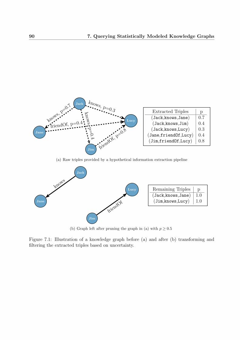
90 7. Querying Statistically Modeled Knowledge Graphs
Lucy
Jim
Jane
Jack
knows,
p=0.7
know
s,p=
0.4
knows, p=0.3
friendOf, p=0.4
frien
dOf,p=0.8
Extracted Triples p(Jack,knows,Jane) 0.7(Jack,knows,Jim) 0.4(Jack,knows,Lucy) 0.3
(Jane,friendOf,Lucy) 0.4(Jim,friendOf,Lucy) 0.8
(a) Raw triples provided by a hypothetical information extraction pipeline
Lucy
Jim
Jane
Jack
knows
frien
dOf
Remaining Triples p(Jack,knows,Jane) 1.0(Jim,knows,Lucy) 1.0
(b) Graph left after pruning the graph in (a) with p ≥ 0.5
Figure 7.1: Illustration of a knowledge graph before (a) and after (b) transforming andfiltering the extracted triples based on uncertainty.
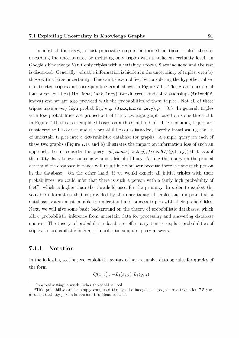
7.1 Exploiting Uncertainty in Knowledge Graphs 91
In most of the cases, a post processing step is performed on these triples, thereby
discarding the uncertainties by including only triples with a sufficient certainty level. In
Google’s Knowledge Vault only triples with a certainty above 0.9 are included and the rest
is discarded. Generally, valuable information is hidden in the uncertainty of triples, even by
those with a large uncertainty. This can be exemplified by considering the hypothetical set
of extracted triples and corresponding graph shown in Figure 7.1a. This graph consists of
four person entities (Jim, Jane, Jack, Lucy), two different kinds of relationships (friendOf,
knows) and we are also provided with the probabilities of these triples. Not all of these
triples have a very high probability, e.g. (Jack, knows, Lucy), p = 0.3. In general, triples
with low probabilities are pruned out of the knowledge graph based on some threshold.
In Figure 7.1b this is exemplified based on a threshold of 0.51. The remaining triples are
considered to be correct and the probabilities are discarded, thereby transforming the set
of uncertain triples into a deterministic database (or graph). A simple query on each of
these two graphs (Figure 7.1a and b) illustrates the impact on information loss of such an
approach. Let us consider the query ∃y.(knows(Jack, y), friendOf(y, Lucy)) that asks if
the entity Jack knows someone who is a friend of Lucy. Asking this query on the pruned
deterministic database instance will result in no answer because there is none such person
in the database. On the other hand, if we would exploit all initial triples with their
probabilities, we could infer that there is such a person with a fairly high probability of
0.662, which is higher than the threshold used for the pruning. In order to exploit the
valuable information that is provided by the uncertainty of triples and its potential, a
database system must be able to understand and process triples with their probabilities.
Next, we will give some basic background on the theory of probabilistic databases, which
allow probabilistic inference from uncertain data for processing and answering database
queries. The theory of probabilistic databases offers a system to exploit probabilities of
triples for probabilistic inference in order to compute query answers.
7.1.1 Notation
In the following sections we exploit the syntax of non-recursive datalog rules for queries of
the form
Q(x, z) : −L1(x, y), L2(y, z)
1In a real setting, a much higher threshold is used.2This probability can be simply computed through the independent-project rule (Equation 7.5); we
assumed that any person knows and is a friend of itself.
92 7. Querying Statistically Modeled Knowledge Graphs
whereQ(x, y) is the head of the rule of queryQ with head variables x and y. L1(x, y), L2(y, z)
is the body of the rule consisting of a conjunction (denoted by the “,”) of the two relational
atoms L1 and L2. As generally used in relational calculus, ∨ and ∧ will denote a logical dis-
junction and conjunction, respectively. Further ∃y will denote the existential quantifier for
the variable y. The active domain ADom of a database is the set of all constants occurring
in the database. Q[a/x] represents the query where the variable x has been substituted by
the constants a where ∀a ∈ a : a ∈ ADom. Further, DomX is the domain of a random
variable X; the set of values that can be assigned to X. Φ will denote a propositional
formula consisting of disjunctions, conjunctions and negation (denoted as ¬) of random
variables. As used in set theory we will denote the union of two sets as⋂
and express a
subset dependency of two sets as ⊆. We will interchangeably use the notation (s, p, o) or
p(s, o) to represent triples, where the latter notation is also referred to as relational tuple.
In that context, p indicates the predicate relation-type and s and o are the subject and
object entities, respectively.
7.1.2 Probabilistic Databases
Probabilistic databases (PDB) have been developed to extend database technologies to
handle uncertain data. A general overview is provided by [100]. PDBs build on the
concept of incomplete databases, which, in contrast to deterministic databases, represent
multiple possible instances (worlds) of a database. One example how these multiple worlds
can emerge is by looking at mutual exclusive relations as the e.g. birthplace relation-
type. Obviously, a person can only have one birthplace, nevertheless it could happen that
in dependence from which document the information is extracted we might get multiple
possible places. An incomplete database would resolve these contradictions by separating
these triples in different possible worlds Wi ∈W, where W is the finite set of all possible
worlds. From an incomplete database we do not know which of the worlds in W is the cor-
rect or exact database instance. Probabilistic databases additionally consider a probability
distributions over these worlds, where∑
Wi∈W P (Wi) = 1, to differentiate these worlds.
Since an explicit representation of all possible worlds is impractical and can be infeasible
if the amount of possible worlds is very large, probabilistic conditional tables (pc-tables) are
used as a representation system. In this representation system each pc-table represents one
relation-type and each tuple t in this table is annotated with a propositional formula Φt ∈ Φ
over mutually independent random variables Xj, where Φ is the set of all propositional
formulas in the database.
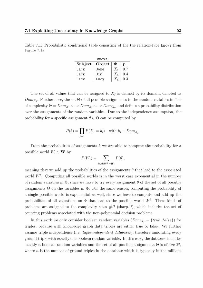
7.1 Exploiting Uncertainty in Knowledge Graphs 93
Table 7.1: Probabilistic conditional table consisting of the the relation-type knows fromFigure 7.1a
knows
Subject Object Φ pJack Jane X1 0.7Jack Jim X2 0.4Jack Lucy X3 0.3
The set of all values that can be assigned to Xj is defined by its domain, denoted as
DomXj . Furthermore, the set Θ of all possible assignments to the random variables in Φ is
of complexity Θ = DomX1×...×DomXj×...×DomXm and defines a probability distribution
over the assignments of the random variables. Due to the independence assumption, the
probability for a specific assignment θ ∈ Θ can be computed by
P (θ) =m∏j=1
P (Xj = bj) with bj ∈ DomXj .
From the probabilities of assignments θ we are able to compute the probability for a
possible world Wi ∈W by
P (Wi) =∑
θ∈Θ:W θ=Wi
P (θ),
meaning that we add up the probabilities of the assignments θ that lead to the associated
world W θ. Computing all possible worlds is in the worst case exponential in the number
of random variables in Φ, since we have to try every assignment θ of the set of all possible
assignments Θ on the variables in Φ. For the same reason, computing the probability of
a single possible world is exponential as well, since we have to compute and add up the
probabilities of all valuations on Φ that lead to the possible world W θ. These kinds of
problems are assigned to the complexity class #P (sharp-P), which includes the set of
counting problems associated with the non-polynomial decision problems.
In this work we only consider boolean random variables (DomXj = {true, false}) for
triples, because with knowledge graph data triples are either true or false. We further
assume triple independence (i.e. tuple-independent databases), therefore annotating every
ground triple with exactly one boolean random variable. In this case, the database includes
exactly n boolean random variables and the set of all possible assignments Θ is of size 2n,
where n is the number of ground triples in the database which is typically in the millions
94 7. Querying Statistically Modeled Knowledge Graphs
to billions.
In Table 7.1, an example PDB representation of the knows relation-type shown in Figure
7.1a using pc-tables is shown. Each subject/object tuple t is annotated with a propositional
formula Φt in this table, which in this case is just the random variable Xt that has been
assigned to the ground triple. Generally the probability p for a tuple t is derived from the
set of satisfying assignments ω(Φt) of the random variables in the propositional formula Φt
with
P (Φt) =∑
θ∈ω(Φt)
P (θ), (7.1)
where for ground tuples, the set of satisfying assignments only consists of Xt = true, which
is the confidence of the e.g. information extractor method used for extracting the triple (re-
lational tuple). For convenience, we have omitted the explicit representation of the counter
events, that is a certain triple is believed to be false, denoted by the propositional formula
¬Xj. Relational tuples can be annotated with more complex propositional formulas, e.g.
after a join of pc-tables. Computing the probability of these formulas can then be reduced
to finding all satisfying assignments, which is also exponential in the number of random
variables in Φt.
The probabilistic database shown in Table 7.1 includes 23 possible worlds. The possible
world W consisting only of the triple (Jack, knows, Jane) can be only generated by the
assignment θ = {X1 = True,X2 = false,X3 = false} and its probability is therefore
given by
P (W ) = P (X1 = true) · P (X2 = false) · P (X3 = false) = 0.7 · 0.6 · 0.7 = 0.294.
In the above example, we started from ground triples which have very simple propo-
sitional formulas (just one random variable). Pc-tables that arose from manipulations of
tables with ground triples, e.g. joins, can lead to very complex propositional formulas for
each tuple t represented in the compound pc-table. The complexity of these propositional
formulas has great impact on the way queries on these databases can be evaluated, since
evaluating queries boils down to evaluating propositional formulas, which is exponential in
the number of random variables. Fortunately, it is possible to sometimes avoid exponen-
tial algorithm runtimes if certain independence assumptions hold on the query structure.
Querying probabilistic databases will be discussed next.
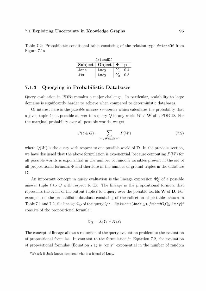
7.1 Exploiting Uncertainty in Knowledge Graphs 95
Table 7.2: Probabilistic conditional table consisting of the relation-type friendOf fromFigure 7.1a
friendOf
Subject Object Φ pJane Lucy Y1 0.4Jim Lucy Y2 0.8
7.1.3 Querying in Probabilistic Databases
Query evaluation in PDBs remains a major challenge. In particular, scalability to large
domains is significantly harder to achieve when compared to deterministic databases.
Of interest here is the possible answer semantics which calculates the probability that
a given tuple t is a possible answer to a query Q in any world W ∈W of a PDB D. For
the marginal probability over all possible worlds, we get
P (t ∈ Q) =∑
W∈W:t∈Q(W )
P (W ) (7.2)
where Q(W ) is the query with respect to one possible world of D. In the previous section,
we have discussed that the above formulation is exponential, because computing P (W ) for
all possible worlds is exponential in the number of random variables present in the set of
all propositional formulas Φ and therefore in the number of ground triples in the database
D.
An important concept in query evaluation is the lineage expression ΦDQ of a possible
answer tuple t to Q with respect to D. The lineage is the propositional formula that
represents the event of the output tuple t to a query over the possible worlds W of D. For
example, on the probabilistic database consisting of the collection of pc-tables shown in
Table 7.1 and 7.2, the lineage ΦQ of the query Q : −∃y.knows(Jack, y), friendOf(y, Lucy)3
consists of the propositional formula:
ΦQ = X1Y1 ∨X2Y2
The concept of lineage allows a reduction of the query evaluation problem to the evaluation
of propositional formulas. In contrast to the formulation in Equation 7.2, the evaluation
of propositional formulas (Equation 7.1) is “only” exponential in the number of random
3We ask if Jack knows someone who is a friend of Lucy.
96 7. Querying Statistically Modeled Knowledge Graphs
variables included in the propositional formula of the lineage (i.e. the set of ground triples
needed for evaluating the query). Further, computing the lineage expression itself for a
query Q(x) with head variables x and a possible tuple a is polynomial in the set of all
constants occurring in the database D (the active domain) and exponential in the number
of variables in the query expression Q 4. As a conclusion, since the size of the lineage
is polynomial in the size of the database and the evaluation of a propositional formula
is exponential in the number of included random variables, the evaluation of the lineage
expression is also in the worst case exponential in the size of the database.
Fortunately, not all queries necessarily lead to an evaluation that is exponential in the
size of D. Often, independence assumption within the query expressions can be exploited
that lead to polynomial query evaluations. Extensional query evaluation is concerned with
queries where the entire probabilistic inference can be computed in a database engine
and thus can be processed as effectively as the evaluation of standard SQL queries. This
queries are denoted as safe. Safe queries can be directly evaluated on query level, with-
out the need to evaluate propositional formulas, except for evaluating the propositional
formulas of ground relational tuples, which are each annotated by a single independent
boolean random variable.5 Queries that are not safe are denoted as unsafe. These queries
can be evaluated by exploiting intensional query evaluation, which evaluates the proposi-
tional formulas. Every relational query can be evaluated this way, but the data complexity
depends dramatically on the query being evaluated, and can be hard for #P .6 Never-
theless, even though some queries might require intensional query evaluation, extensional
query evaluation sometimes might provide a good approximate that suffices for the target
application.
For our contribution, we will focus on extensional query evaluation and safe queries,
respectively, because they are of major importance for the contributions of this chapter.
Intensional query evaluation is not a target of this chapter and we refer to [100], Chapter
5 for details on intensional query evaluation using rules or circuits.
4Not to be confused with the number of random variables in ΦQ(x).5This also holds for more expressive probabilistic databases, since these databases can be decomposed
to tuple-independent databases. [100], Chapter 46Generally all unsafe queries are in #P and all safe queries are polynomial. This is known as the
dichotomy theorem. Nevertheless, due to the notion of the sufficient syntactic independence assumptionwe might classify certain safe queries as unsafe and perform intensional query evaluation.

7.1 Exploiting Uncertainty in Knowledge Graphs 97
Extensional Query Evaluation
Extensional query evaluation only depends on the query expression itself and the lineage
does not need to be computed. During the evaluation process, several rules are applied to
the query in order to divide it into smaller and easier sub-queries until it reduces to ground
tuples with elementary probability values. Queries that can be completely simplified to
ground tuples with extensional evaluation rules are safe, in the sense mentioned above.
This evaluation procedure relies on identifying independent probabilistic events in the
query that can be separated, e.g. in case of a join into a conjunction of two simpler queries,
where the probabilities of the two sub-queries can simply be multiplied.
It can be decided that two queries are independent probabilistic events if they are
syntactically independent. Syntactic independence of two propositional formulas ΦQ1 and
ΦQ2 is given if V ar(ΦQ1)∩V ar(ΦQ2) = ∅, where V ar(Φ) denotes the set of random variables
Φ depends on (known as the support of Φ). Unfortunately, the determination of the support
of a propositional formula is in general co-NP-complete. In extensional query evaluation it
often suffices to exploit a sufficient condition for syntactic independence for this purpose
which can determine if queries are independent probabilistic events in polynomial time.
The sufficient condition syntactic independence is given by V (ΦQ1) ∩ V (ΦQ2) = ∅, where
V (Φ) denotes the set of random variables that are observed in Φ. Clearly, V ar(ΦQ1) ⊆V (Φ) and therefore propositional formulas that fulfill the sufficient condition for syntactic
independence are also syntactically independent (but the converse does not hold). In tuple-
independent databases, each ground tuple is associated with a random variable. Therefore
two sub-queries Q1 and Q2 are guaranteed to be independent probabilistic events if they
do not unify, meaning that they share no common tuple.7 Note that it can be decided if
two sub-queries are independent solely based on the query syntax without the need of the
lineage expression.
Extensional query evaluation can be implemented via the application of six rules [100],
with three of them, especially the independent-project rule, being of major importance for
the remaining chapter.
• Independent Join:
P (Q1 ∧Q2) = P (Q1) · P (Q2) (7.3)
7Due to the absorption law, there can be syntactically independent queries that unify.
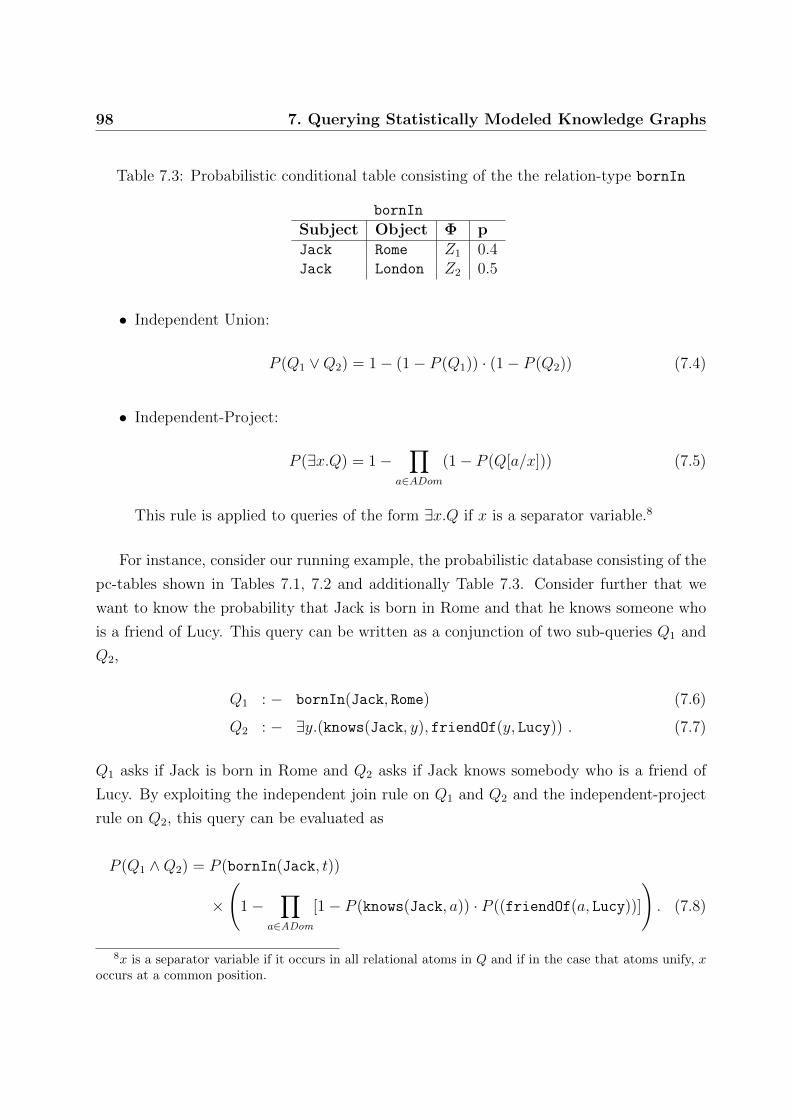
98 7. Querying Statistically Modeled Knowledge Graphs
Table 7.3: Probabilistic conditional table consisting of the the relation-type bornIn
bornIn
Subject Object Φ pJack Rome Z1 0.4Jack London Z2 0.5
• Independent Union:
P (Q1 ∨Q2) = 1− (1− P (Q1)) · (1− P (Q2)) (7.4)
• Independent-Project:
P (∃x.Q) = 1−∏
a∈ADom
(1− P (Q[a/x])) (7.5)
This rule is applied to queries of the form ∃x.Q if x is a separator variable.8
For instance, consider our running example, the probabilistic database consisting of the
pc-tables shown in Tables 7.1, 7.2 and additionally Table 7.3. Consider further that we
want to know the probability that Jack is born in Rome and that he knows someone who
is a friend of Lucy. This query can be written as a conjunction of two sub-queries Q1 and
Q2,
Q1 : − bornIn(Jack, Rome) (7.6)
Q2 : − ∃y.(knows(Jack, y), friendOf(y, Lucy)) . (7.7)
Q1 asks if Jack is born in Rome and Q2 asks if Jack knows somebody who is a friend of
Lucy. By exploiting the independent join rule on Q1 and Q2 and the independent-project
rule on Q2, this query can be evaluated as
P (Q1 ∧Q2) = P (bornIn(Jack, t))
×
(1−
∏a∈ADom
[1− P (knows(Jack, a)) · P ((friendOf(a, Lucy))]
). (7.8)
8x is a separator variable if it occurs in all relational atoms in Q and if in the case that atoms unify, xoccurs at a common position.
7.2 Exploiting Latent Variable Models for Querying 99
Note that a person can know many other persons and therefore the knows relations in Q2
are not mutually exclusive. This induces a complex expression that is not simply the sum
or the product of probabilities.
7.2 Exploiting Latent Variable Models for Querying
As discussed in the introduction for this chapter, we can exploit latent variable models
for learning a probability distribution over all possible triples (with considering type-
constraints) of the knowledge graph. This probability distribution can be exploited for
constructing a probabilistic database. The naive approach for realizing probabilistic query-
ing on this database would be to infer all probabilities from the latent variable model and
save them in the database together with the corresponding triples. Then, we could query
this database as any other probabilistic database, exploiting extensional and intensional
query evaluation algorithms.
Obviously, this approach is intractable for larger knowledge graphs, because the amount
of possible triples is simply too large. The Freebase sample shown in Table 4.2 contains
already 57 billion possible triples and saving these triples together with the probabilities
would consume approximately 1TB of storage9. Note that this sample is considerably small
compared to whole Freebase, e.g. it contains only 0.3% of the Topic entities and 0.4% of
the relation-types of Freebase (see Chapter 2.3.2).
As an alternative, we could compute the probabilities “on demand” for those triples
that are of interest for the current query or sub-query and apply the query evaluation
rules afterwards. This approach would avoid storage explosion, but introduces additional
computational load on the query evaluation, which can be tremendous. Note that no
matter if the query is safe or unsafe we would have to compute |V ar(ΦQ)| probabilities,
which is the number of random variables (i.e. ground triples) the query depends on. Below,
we exemplify this issue based on a series of simple safe queries.
Consider the relational tuple knows(Jane, Jim). The probability of this relation is
computed from a latent variable model θ (any of the methods described in Chapter 3.3)
by
P (knows(Jane, Jim)) = ψ(θJane,knows,Jim),
where θs,p,o denotes the confidence of the latent variable model into the relation that Jane
9Considering that each triple is saved by 32 bit integer values and the probability by one 32 bit floatvalue.
100 7. Querying Statistically Modeled Knowledge Graphs
knows Jim and ψ(x) ∈ (0, 1] maps this confidence value to a valid probability space through
e.g. Platt Scaling (see Equation 6.2 or [87]).
If we need to know the probability that anybody knows Jim (Q : −∃y.knows(y, Jim)
we would have to compute |ADom| evaluations of the latent variable model. If we further
assume the query
Q : −∃y.knows(Jack, y), friendOf(y, Lucy),
which is evaluated by applying the independent-project rule as
P (Q) =
(1−
∏a∈ADom
[1− P (knows(Jack, a)) · P ((friendOf(a, Lucy))]
),
we can observe that it needs 2×|ADom| evaluations of the latent variable model. In many
cases it can also be of interest to extract a ranking over all persons in the database that
are a friend of Lucy with
Q(x) : −∃y.knows(x, y), friendOf(y, Lucy),
to get the persons that most likely know friends of the entity. For his query we would need
2 × |ADom|2 evaluations of the latent variable model. The structure of the above query
can even lead to cubic evaluations in |ADom| of the model, if we modify the query to
Q(x) : −∃y.(knows(x, y),∃z.friendOf(y, z)),
where we introduced another existential quantifier for the second variable in the relation-
type friendOf by querying for all persons that know someone who has friends. This query
is evaluated as
P (Q(x)) =
(1−
∏a1∈ADom
[1− P (knows(x, a1)) ·
(1−
∏a2∈ADom
[1− P (friendOf(a1, a2))
))
The complexity is mainly caused by nested computations introduced by the existentially
quantified query variables and their product-aggregation in the independent-project rule
(Equation (7.5)).
It is expected that the computation of the probabilities from the latent variable models
will have significant negative impact on the total query evaluation time, especially when
evaluating with the independent-project rule.
7.2 Exploiting Latent Variable Models for Querying 101
The key idea is to reduce the amount of evaluations of latent variable models through
approximating safe sub-queries of the type ∃x.Q by exploiting intrinsic features of latent
variable models. Through this approach, we avoid costly evaluations of sub-queries and ad-
ditionally construct materialized views that have a memory efficient latent representation.
To illustrate the proposed approach, consider the queries Q1 and Q2 from Equations 7.6
and 7.7. Q1 does not include any existential quantifier and therefore we simply compute
the probability value from the model. In Q2, an existential quantifier for the variable y is
present. As discussed before, the calculation of queries that have a similar structure as Q2
can become very expensive. To overcome this problem, we approximate the probabilistic
answer to Q2 by a two-step process. First, we create a newly formed compound relation
knowsFriendOf, which represents the database view generated by Q2,
Q2(x, z) : −knowsFriendOf(x, z).
To create the compound relation, we use the deterministic and sparse representation of the
affected relations from Q2 and join them into a single relation. This avoids the expensive
calculation of probabilities for each instance of the active domain of y and can be computed
efficiently, as the deterministic join is not expensive, if the (deterministic) domain is sparse.
However, the representation of Q2 would only be based on the available deterministic
information so far and would not utilize the probabilistic model of the knowledge graph
computed by the latent variable model. Hence, in a second step we now need to derive
probabilities for the triples in the newly formed compound relation. Fortunately, all that
is needed to derive these probabilities under a latent variable model such as RESCAL
or TransE is to compute a latent representation of the newly created compound relation
knowsFriendOf, which can be done very efficiently.10 Depending on the latent variable
model, the procedure for learning the latent representation of the compound relation differs.
In the next subsection we will describe how a new compound relation can be learned with
RESCAL, TransE and the multiway neural network approach exploited in the Google
Knowledge Vault project (mwNN).
10Note that it is assumed for the new compound relation that all triples are independent and for thisreason it can be exploited as view. Generally, extensional query evaluation exploits the possible answerssemantics which is not compositional, meaning that the computed probabilities do not represent a proba-bilistic database, but a collection of probabilities that cannot be exploited for further querying.
102 7. Querying Statistically Modeled Knowledge Graphs
7.2.1 Learning Compound Relations with RESCAL
Let X(∗) denote the newly created type-constrained compound relation and domain(∗)
and range(∗) its domain and range, which can be easily derived from the joined relation-
types. Furthermore, assume that a meaningful latent representation of the entities has
been explored via the factorization of the deterministic triple store. Since the RESCAL
model uses a unique representation of entities over all relations, all that is needed to
derive probabilities for a new relation is to compute its latent representation R(∗). The big
advantage of the proposed method is that R(∗) can now be derived by simply projecting
X(∗) into the latent space that is spanned by the type-constrained embedding matrices
of entities A[domain(∗),:]and A[range(∗),:]
. This can be done very efficiently. Consider the
type-constrained ALS update for the core tensor R from Chapter 5.1.2. Essentially, what
is necessary is to calculate the latent matrix for the materialized view, i.e., R(∗) as
R(∗) = ((C⊗B)T (C⊗B) + λI)−1(C⊗B)Tvec(Xk) (7.9)
with B = A[domain(∗),:]and C = A[range(∗),:].
It was shown in Chapter 5.1.2 that this closed-form solution can be calculated more effi-
ciently by exploiting the singular value decomposition of the type-constrained factor ma-
trices A[domain(∗),:]= UBΣBVT
B and A[range(∗),:]= UCΣCVT
C, leading to
R(∗) = VB(P ~ UTBX(∗)UC)VT
C (7.10)
where ~ represents the Hadamard (element-wise) matrix product and P has been defined
as follows (Chapter 5.1.2): Let Q be defined as a diagonal matrix and its diagonal entry
qii be given by
qii =DBiiDCii
D2Bii
D2Cii
+ λ
with DB = ΣB ⊗ ΣB and DC = ΣC ⊗ ΣC.
Then P can be constructed by a column-wise reshape of the diagonal in Q.
The calculation of the latent representation R(∗) for the newly created compound
relation-type can now be done in O(r3 + n(∗)r +m(∗)r + pr), where p represents the num-
ber of nonzero entries in X(∗), r represents the rank of the factorization, and where n(∗)
represents all entities in the domain and m(∗) represents all entities in the range of the
7.2 Exploiting Latent Variable Models for Querying 103
compound relation-type (∗). Please note that the computation of R(∗) is now linear in all
parameters regarding the size of the triple store and cubic only in the number of latent
components r that are used to factorize the triple store. As such, it can be computed
efficiently even for very large triple stores. Furthermore, for each query of the same type,
the same latent representation can be reused, i.e. R(∗) only needs to be computed once.
7.2.2 Learning Compound Relations with TransE and mwNN
Similar to RESCAL, we are also able to learn new latent representations for compound
relation-types with TransE and mwNN, but in contrast to RESCAL we are not able to
exploit a closed-form solution for this. Let again X(∗) denote the newly created compound
relation with type-constraints domain(∗) and range(∗), which have been derived from the
joined relation-types. We also assume that the latent representations for the entities have
been inferred from a sufficient amount of data such that they are stable. In other words, we
assume that we have already found good representations for entities. Further, in case of the
neural network model, we also assume that the network weights have reached a stable local
minimum. We then learn the new representation of the compound relation-type through
stochastic gradient descent considering all model parameters as constant except for the
new latent representation r(∗). Below, we will provide the update rules for both models,
TransE and mwNN, for learning r(∗).
Updating r(∗) with TransE
For each triple (s, (∗), o) drawn from the compound relation (∗), the loss function of TransE
is given as
LT C(∗)TransE = max{0, γ + θs′,(∗),o − θs,(∗),o}+ max{0, γ + θs,(∗),o′ − θs,(∗),o} (7.11)
where s′ ∈ E[domain(∗)] ⊆ E , o′ ∈ E[range(∗)] ⊆ E ,
and where for any triple (s, p, o), θs,p,o = −δ(as + rp, ao).
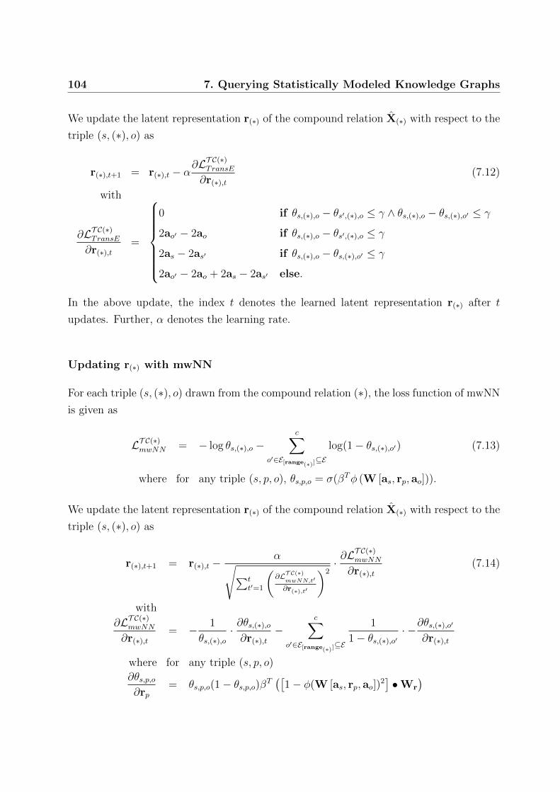
104 7. Querying Statistically Modeled Knowledge Graphs
We update the latent representation r(∗) of the compound relation X(∗) with respect to the
triple (s, (∗), o) as
r(∗),t+1 = r(∗),t − α∂LT C(∗)TransE
∂r(∗),t(7.12)
with
∂LT C(∗)TransE
∂r(∗),t=
0 if θs,(∗),o − θs′,(∗),o ≤ γ ∧ θs,(∗),o − θs,(∗),o′ ≤ γ
2ao′ − 2ao if θs,(∗),o − θs′,(∗),o ≤ γ
2as − 2as′ if θs,(∗),o − θs,(∗),o′ ≤ γ
2ao′ − 2ao + 2as − 2as′ else.
In the above update, the index t denotes the learned latent representation r(∗) after t
updates. Further, α denotes the learning rate.
Updating r(∗) with mwNN
For each triple (s, (∗), o) drawn from the compound relation (∗), the loss function of mwNN
is given as
LT C(∗)mwNN = − log θs,(∗),o −c∑
o′∈E[range(∗)]⊆E
log(1− θs,(∗),o′) (7.13)
where for any triple (s, p, o), θs,p,o = σ(βTφ (W [as, rp, ao])).
We update the latent representation r(∗) of the compound relation X(∗) with respect to the
triple (s, (∗), o) as
r(∗),t+1 = r(∗),t −α√∑t
t′=1
(∂LT C(∗)
mwNN,t′
∂r(∗),t′
)2· ∂L
T C(∗)mwNN
∂r(∗),t(7.14)
with
∂LT C(∗)mwNN
∂r(∗),t= − 1
θs,(∗),o·∂θs,(∗),o∂r(∗),t
−c∑
o′∈E[range(∗)]⊆E
1
1− θs,(∗),o′· −
∂θs,(∗),o′
∂r(∗),t
where for any triple (s, p, o)
∂θs,p,o∂rp
= θs,p,o(1− θs,p,o)βT([
1− φ(W [as, rp, ao])2]•Wr
)
7.2 Exploiting Latent Variable Models for Querying 105
Again, the index t denotes the learned latent representation r(∗) after t updates and in
Equation 7.14 the fraction incorporating the learning rate α describes the adaptive learning
rate [26]. Wr denotes only that part of the weight matrix W that interacts with the
latent representations of relation-types in the matrix product W [as, rp, ao]. • denotes the
column-wise product between a vector and a matrix.
7.2.3 Numerical Advantage of Learned Compound Relation-Types
In addition to the decrease in evaluations of the latent variable model to generate the
required probabilities there is also a numerical advantage of the learned compound relation
regarding its probabilities. Consider the query
Q(x) : −∃y.knows(x, y), friendOf(y, Lucy),
which can be evaluated with the independent-project rule as
P (Q(x)) =
(1−
∏a∈ADom
[1− P (knows(x, a)) · P ((friendOf(a, Lucy))]
).
For relation-types with a large domain or range, the above product can range over thou-
sands of different values of a, namely all entities that are in common by the range of the
first relation-type (in the above example knows) and the domain of the second relation-
type (friendOf in the above example). As a consequence, the product of all probabilities∏a∈ADom[1− P (knows(x, a)) · P ((friendOf(a, Lucy))] will quickly evolve beyond machine
precision. As a simple example, assume that the above product loops over 10,000 entities.
It makes no difference if the probabilities 1 − P (knows(x, a)) · P ((friendOf(a, Lucy)) are
all 0.99 or 0.01. The probability for the query P (Q(x)) will be exactly 1.0 for any x.
Obviously, ranking the results is pointless in this case. Note that due to the structure of
the independent-project rule, substituting the product of probabilities through the sum of
logarithmic probabilities,
P (Q) = 1− exp(∑
a∈ADom
log(1− P (knows(Jack, a)) · P ((friendOf(a, Lucy)))),
does not provide a solution for this problem because the exponent will be a very large
negative value.
The learned compound relation-types on the other hand will contain probabilities that
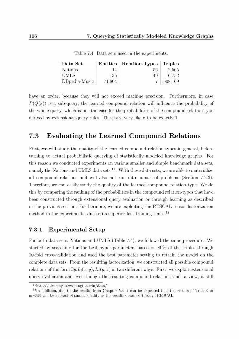
106 7. Querying Statistically Modeled Knowledge Graphs
Table 7.4: Data sets used in the experiments.
Data Set Entities Relation-Types TriplesNations 14 56 2,565UMLS 135 49 6,752DBpedia-Music 71,804 7 508,169
have an order, because they will not exceed machine precision. Furthermore, in case
P (Q(x)) is a sub-query, the learned compound relation will influence the probability of
the whole query, which is not the case for the probabilities of the compound relation-type
derived by extensional query rules. These are very likely to be exactly 1.
7.3 Evaluating the Learned Compound Relations
First, we will study the quality of the learned compound relation-types in general, before
turning to actual probabilistic querying of statistically modeled knowledge graphs. For
this reason we conducted experiments on various smaller and simple benchmark data sets,
namely the Nations and UMLS data sets 11. With these data sets, we are able to materialize
all compound relations and will also not run into numerical problems (Section 7.2.3).
Therefore, we can easily study the quality of the learned compound relation-type. We do
this by comparing the ranking of the probabilities in the compound relation-types that have
been constructed through extensional query evaluation or through learning as described
in the previous section. Furthermore, we are exploiting the RESCAL tensor factorization
method in the experiments, due to its superior fast training times.12
7.3.1 Experimental Setup
For both data sets, Nations and UMLS (Table 7.4), we followed the same procedure. We
started by searching for the best hyper-parameters based on 80% of the triples through
10-fold cross-validation and used the best parameter setting to retrain the model on the
complete data sets. From the resulting factorization, we constructed all possible compound
relations of the form ∃y.Li(x, y), Lj(y, z) in two different ways. First, we exploit extensional
query evaluation and even though the resulting compound relation is not a view, it still
11http://alchemy.cs.washington.edu/data/12In addition, due to the results from Chapter 5.4 it can be expected that the results of TransE or
mwNN will be at least of similar quality as the results obtained through RESCAL.
7.3 Evaluating the Learned Compound Relations 107
represents valid probabilities of each triple in the compound relation. Second, we learn the
compound relation-types as views as described in Section 7.2.1 (Equation 7.10).
For the comparison of both approaches, we assume that the extensional query evalua-
tion results in a correct ranking of probabilities in the compound relation-type (our gold
standard). For this reason we binarize the compound relation-type derived through exten-
sional query evaluation, where the top k triples with the highest probability are assumed
true (or one) and the other are assumed as false (or zero). We define k as the number
of true triples in the deterministic compound relation between the deterministic versions
of the relation-types Li and Lj. We then compare the ranking of triples in the learned
compound relation to the above defined gold standard derived from the extensional query
evaluation in terms of the Area Under the Precision Recall Curve (AUPRC). In addition,
we also report the results when comparing the gold standard against a random ranking.
For each compound relation we repeated the comparison against random ten times and
used the median as final score.
We report the median13 and standard deviation of the AUPRC scores on all possible
compound relation-types (without self joins), where we only considered compound relations
that contained more than 10 triples.
7.3.2 Compound Relations are of Good Quality
In Figures 7.2 and 7.3 the results for the Nations and UMLS data sets are shown. Generally,
the compound relation-types learned from the deterministic compound relation-type result
in a very similar ranking as the compound relation-type obtained by the extensional query
evaluation rules, which served as gold standard.
In case of the Nations data set, 2,354 compound relations were evaluated. The ranking
in the learned compound relation-type agrees with the ranking of the gold standard with a
median AUPRC score of 0.8248 and for 83 compound relation-types the AUPRC score is
above 0.99 (standard deviation is 0.2174). The ranking of a random relation-type on the
other hand results in clearly less agreement with the gold standard (grey bar), as expected.
For the UMLS data set, 631 compound relation-types were evaluated. In this case,
we have strong agreement between both kinds of compound relation-types, the learned
compound relation and the one derived through extensional query evaluation. The median
AUPRC score is almost perfect (0.9970) and clearly differs from the agreement achieved
by a random relation-type (AUPRC:0.0034).
13We report the median because of its robustness to outliers.
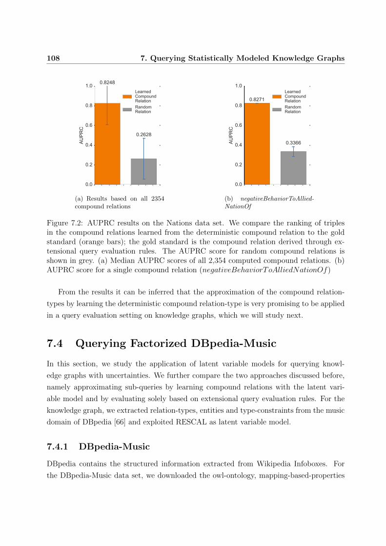
108 7. Querying Statistically Modeled Knowledge Graphs
0.0
0.2
0.4
0.6
0.8
1.0AU
PRC
0.8248
0.2628
LearnedCompoundRelationRandomRelation
(a) Results based on all 2354compound relations
0.0
0.2
0.4
0.6
0.8
1.0
AUPR
C
0.8271
0.3366
LearnedCompoundRelationRandomRelation
(b) negativeBehaviorToAllied-NationOf
Figure 7.2: AUPRC results on the Nations data set. We compare the ranking of triplesin the compound relations learned from the deterministic compound relation to the goldstandard (orange bars); the gold standard is the compound relation derived through ex-tensional query evaluation rules. The AUPRC score for random compound relations isshown in grey. (a) Median AUPRC scores of all 2,354 computed compound relations. (b)AUPRC score for a single compound relation (negativeBehaviorToAlliedNationOf)
From the results it can be inferred that the approximation of the compound relation-
types by learning the deterministic compound relation-type is very promising to be applied
in a query evaluation setting on knowledge graphs, which we will study next.
7.4 Querying Factorized DBpedia-Music
In this section, we study the application of latent variable models for querying knowl-
edge graphs with uncertainties. We further compare the two approaches discussed before,
namely approximating sub-queries by learning compound relations with the latent vari-
able model and by evaluating solely based on extensional query evaluation rules. For the
knowledge graph, we extracted relation-types, entities and type-constraints from the music
domain of DBpedia [66] and exploited RESCAL as latent variable model.
7.4.1 DBpedia-Music
DBpedia contains the structured information extracted from Wikipedia Infoboxes. For
the DBpedia-Music data set, we downloaded the owl-ontology, mapping-based-properties
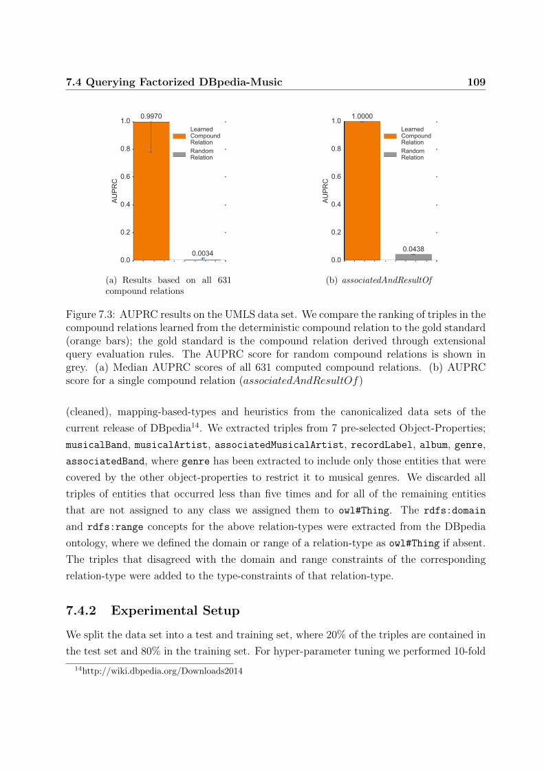
7.4 Querying Factorized DBpedia-Music 109
0.0
0.2
0.4
0.6
0.8
1.0AU
PRC
0.9970
0.0034
LearnedCompoundRelationRandomRelation
(a) Results based on all 631compound relations
0.0
0.2
0.4
0.6
0.8
1.0
AUPR
C
1.0000
0.0438
LearnedCompoundRelationRandomRelation
(b) associatedAndResultOf
Figure 7.3: AUPRC results on the UMLS data set. We compare the ranking of triples in thecompound relations learned from the deterministic compound relation to the gold standard(orange bars); the gold standard is the compound relation derived through extensionalquery evaluation rules. The AUPRC score for random compound relations is shown ingrey. (a) Median AUPRC scores of all 631 computed compound relations. (b) AUPRCscore for a single compound relation (associatedAndResultOf)
(cleaned), mapping-based-types and heuristics from the canonicalized data sets of the
current release of DBpedia14. We extracted triples from 7 pre-selected Object-Properties;
musicalBand, musicalArtist, associatedMusicalArtist, recordLabel, album, genre,
associatedBand, where genre has been extracted to include only those entities that were
covered by the other object-properties to restrict it to musical genres. We discarded all
triples of entities that occurred less than five times and for all of the remaining entities
that are not assigned to any class we assigned them to owl#Thing. The rdfs:domain
and rdfs:range concepts for the above relation-types were extracted from the DBpedia
ontology, where we defined the domain or range of a relation-type as owl#Thing if absent.
The triples that disagreed with the domain and range constraints of the corresponding
relation-type were added to the type-constraints of that relation-type.
7.4.2 Experimental Setup
We split the data set into a test and training set, where 20% of the triples are contained in
the test set and 80% in the training set. For hyper-parameter tuning we performed 10-fold
14http://wiki.dbpedia.org/Downloads2014
110 7. Querying Statistically Modeled Knowledge Graphs
cross-validation on the training set. The final model is trained on the complete training set
with the best hyper-parameters. We exploit this model for evaluating the various queries
on the DBpedia-Music data set in two ways:
1. We evaluate the queries solely based on extensional query evaluation rules, using the
probabilities generated by the trained model.
2. We evaluate the same queries based on extensional query evaluation rules, but with
additionally approximating suitable sub-queries by learning the compound relation-
type from the deterministic version of the compound relation with the latent variable
model (RESCAL).
The quality of the answers (the ranking of probabilities) generated by the two query
evaluation approaches is evaluated against three ground truths:
1. The deterministic answers of the database consisting of the training set. We evaluate
the inference of known answers.
2. The deterministic answers which were not included in the training set (answers of
(test set ∪ training set) \ answers of training set). We evaluate the inference of new
answers.
3. The deterministic answers of the database consisting of the whole data sets (answers
of (test set ∪ training set)). We evaluate the total inference quality.
We measure the AUPRC, AUROC and the Logarithmic Loss. The Logarithmic Loss,
logloss = − 1
N
N∑i=1
(yilog(pi) + (1− yi)log(1− pi)) ,
is widely used to evaluate the quality of the probabilities generated by statistical models,
whereas in difference to the AUPRC and AUROC a better performance is indicated by a
lower value.
We further compare the computation time when evaluating the queries purely rule
based with the evaluation procedure where we exploit extensional rules and approximate
sub-queries through compound relations learned by the model. All models are implemented
in python and the runtime measurements were taken with an Intel(R) Xeon(R) CPU E7-
4850 v2. We factorized the knowledge graph data with RESCAL using a rank of 200.
7.4 Querying Factorized DBpedia-Music 111
7.4.3 Queries Used for Evaluation
We will now describe the various queries used for the experiments and also give details to
their computation.
1. What songs or albums from the Pop-Rock genre are from musical artists that have/had
a contract with Atlantic Records?
Q1(x) : −genre(x,Pop rock)∧
∃y.(musicalArtist(x, y) ∧ recordLabel(y,Atlantic Records)).
This query is evaluated by extensional query evaluation rules as
Q1(x) = P (genre(x, z))×[1−
∏b∈ADom
1− P (musicalArtist(x, b) · P (recordLabel(b,Atlantic Records))
].
and by exploiting the learned compound relation songsAndAlbumsFromRecordLabel
learned from compound relation consisting of the relation-types musicalArtist and
recordLabel as
Q1(x) = P (genre(x,PopRock))×
P (songsAndAlbumsFromRecorLabel(x,Atlantic Records)) ,
2. Which musical artists from the Hip Hop music genre were involved in a single that
was produced by Shady (SD), Aftermath (AM) or Death Row (DR) records?
Q2(x) : −∃y.(genre(x, {Hip hop music,Hip hop})∧
musicalArtist(y, x) ∧ recordLabel(y, {SD,AM,DR}))
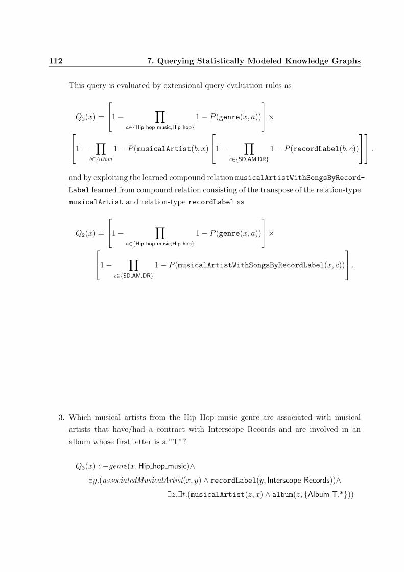
112 7. Querying Statistically Modeled Knowledge Graphs
This query is evaluated by extensional query evaluation rules as
Q2(x) =
1−∏
a∈{Hip hop music,Hip hop}
1− P (genre(x, a))
×1−
∏b∈ADom
1− P (musicalArtist(b, x)
1−∏
c∈{SD,AM,DR}
1− P (recordLabel(b, c))
.and by exploiting the learned compound relation musicalArtistWithSongsByRecord-
Label learned from compound relation consisting of the transpose of the relation-type
musicalArtist and relation-type recordLabel as
Q2(x) =
1−∏
a∈{Hip hop music,Hip hop}
1− P (genre(x, a))
×1−
∏c∈{SD,AM,DR}
1− P (musicalArtistWithSongsByRecordLabel(x, c))
.
3. Which musical artists from the Hip Hop music genre are associated with musical
artists that have/had a contract with Interscope Records and are involved in an
album whose first letter is a ”T”?
Q3(x) : −genre(x,Hip hop music)∧
∃y.(associatedMusicalArtist(x, y) ∧ recordLabel(y, Interscope Records))∧
∃z.∃t.(musicalArtist(z, x) ∧ album(z, {Album T.*}))
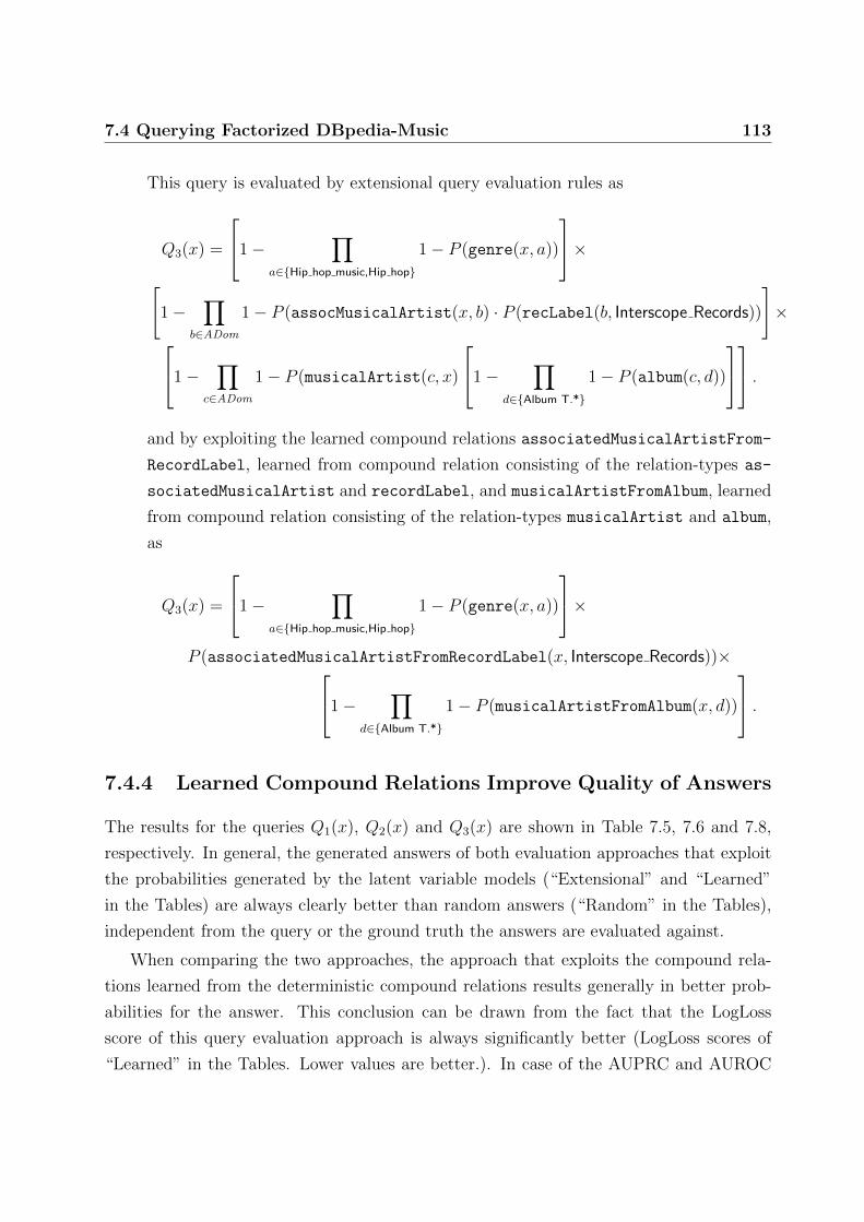
7.4 Querying Factorized DBpedia-Music 113
This query is evaluated by extensional query evaluation rules as
Q3(x) =
1−∏
a∈{Hip hop music,Hip hop}
1− P (genre(x, a))
×[
1−∏
b∈ADom
1− P (assocMusicalArtist(x, b) · P (recLabel(b, Interscope Records))
]×1−
∏c∈ADom
1− P (musicalArtist(c, x)
1−∏
d∈{Album T.*}
1− P (album(c, d))
.and by exploiting the learned compound relations associatedMusicalArtistFrom-
RecordLabel, learned from compound relation consisting of the relation-types as-
sociatedMusicalArtist and recordLabel, and musicalArtistFromAlbum, learned
from compound relation consisting of the relation-types musicalArtist and album,
as
Q3(x) =
1−∏
a∈{Hip hop music,Hip hop}
1− P (genre(x, a))
×P (associatedMusicalArtistFromRecordLabel(x, Interscope Records))×1−
∏d∈{Album T.*}
1− P (musicalArtistFromAlbum(x, d))
.7.4.4 Learned Compound Relations Improve Quality of Answers
The results for the queries Q1(x), Q2(x) and Q3(x) are shown in Table 7.5, 7.6 and 7.8,
respectively. In general, the generated answers of both evaluation approaches that exploit
the probabilities generated by the latent variable models (“Extensional” and “Learned”
in the Tables) are always clearly better than random answers (“Random” in the Tables),
independent from the query or the ground truth the answers are evaluated against.
When comparing the two approaches, the approach that exploits the compound rela-
tions learned from the deterministic compound relations results generally in better prob-
abilities for the answer. This conclusion can be drawn from the fact that the LogLoss
score of this query evaluation approach is always significantly better (LogLoss scores of
“Learned” in the Tables. Lower values are better.). In case of the AUPRC and AUROC
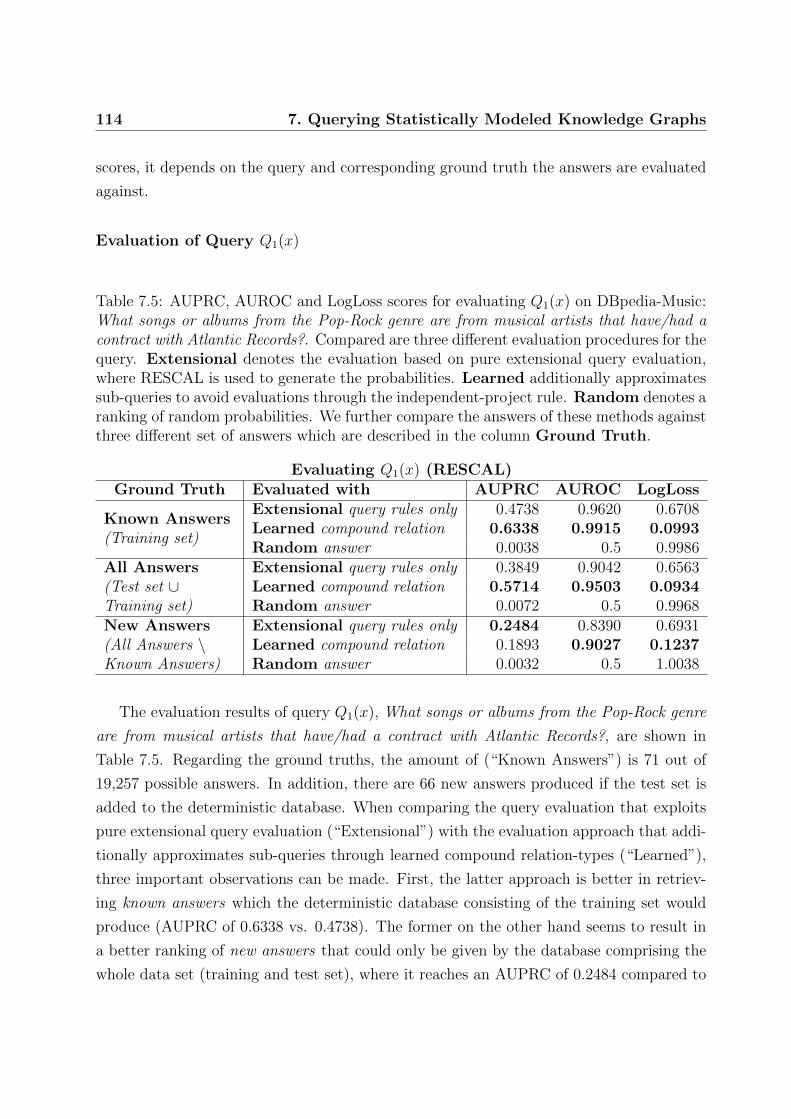
114 7. Querying Statistically Modeled Knowledge Graphs
scores, it depends on the query and corresponding ground truth the answers are evaluated
against.
Evaluation of Query Q1(x)
Table 7.5: AUPRC, AUROC and LogLoss scores for evaluating Q1(x) on DBpedia-Music:What songs or albums from the Pop-Rock genre are from musical artists that have/had acontract with Atlantic Records?. Compared are three different evaluation procedures for thequery. Extensional denotes the evaluation based on pure extensional query evaluation,where RESCAL is used to generate the probabilities. Learned additionally approximatessub-queries to avoid evaluations through the independent-project rule. Random denotes aranking of random probabilities. We further compare the answers of these methods againstthree different set of answers which are described in the column Ground Truth.
Evaluating Q1(x) (RESCAL)Ground Truth Evaluated with AUPRC AUROC LogLoss
Extensional query rules only 0.4738 0.9620 0.6708Learned compound relation 0.6338 0.9915 0.0993
Known Answers(Training set)
Random answer 0.0038 0.5 0.9986Extensional query rules only 0.3849 0.9042 0.6563Learned compound relation 0.5714 0.9503 0.0934
All Answers(Test set ∪Training set) Random answer 0.0072 0.5 0.9968
Extensional query rules only 0.2484 0.8390 0.6931Learned compound relation 0.1893 0.9027 0.1237
New Answers(All Answers \Known Answers) Random answer 0.0032 0.5 1.0038
The evaluation results of query Q1(x), What songs or albums from the Pop-Rock genre
are from musical artists that have/had a contract with Atlantic Records?, are shown in
Table 7.5. Regarding the ground truths, the amount of (“Known Answers”) is 71 out of
19,257 possible answers. In addition, there are 66 new answers produced if the test set is
added to the deterministic database. When comparing the query evaluation that exploits
pure extensional query evaluation (“Extensional”) with the evaluation approach that addi-
tionally approximates sub-queries through learned compound relation-types (“Learned”),
three important observations can be made. First, the latter approach is better in retriev-
ing known answers which the deterministic database consisting of the training set would
produce (AUPRC of 0.6338 vs. 0.4738). The former on the other hand seems to result in
a better ranking of new answers that could only be given by the database comprising the
whole data set (training and test set), where it reaches an AUPRC of 0.2484 compared to
7.4 Querying Factorized DBpedia-Music 115
0.1893 of the other approach.
Second, from the AUROC scores we can infer that the approach that exploits the
learned compound relations has a slightly better recall than the approach that relies solely
on extensional query evaluation. For the known answers it achieves an AUROC of 0.9915
and for new answers 0.9027, whereas the “Extensional” evaluation reaches only 0.9620 and
0.8390.
Third, as mentioned early, both evaluation approaches differ significantly in their
LogLoss scores. The evaluation with learned compound relation clearly outperforms the
other method with a logloss score of 0.0993 for known answers and 0.1237 for new answers,
whereas pure extensional query evaluation is 0.6708 and 0.6931. This has a significant
impact on the interpretation of the AUPRC score. We can conclude that even though the
evaluation with learned compound relations results in a worse ranking, the resulting prob-
abilities are much more meaningful. Meaningful probabilities allow us to easily filter the
answers generated by the evaluation approach, discarding answers with lower probability.
In other words, we can directly determine if an answer is likely to be wrong.
Evaluation of Query Q2(x)
The evaluation results of query Q2(x), Which musical artists from the Hip Hop music
genre involved in a single that was produced by Shady, Aftermath or Death Row records?,
are shown in Table 7.6. The deterministic ground truths consist of 28 (“Known An-
swers”) out of 23,269 possible answers and the test set resulted in 8 additional “New
Answers” (36 answers in total). The results are very similar to query Q1(x) when compar-
ing the query evaluation with extensional rules only, with the approach that exploits the
learned compound relation to partially avoid expensive evaluations of sub-queries with the
independent-project rule. Again, the LogLoss score is significantly better, but it is also
notable that a really low AUPRC score can be observed for the latter approach (0.0194).
From the top 25 ranking of this evaluation method on this query shown in Table 7.7, it
can be inferred that the low AUPRC is very likely caused by incompleteness of the corre-
sponding deterministic DBpedia-Music knowledge graph. The answers (rows) that are not
highlighted are present in the ground truth generated from the whole data (training set
∪ test set). The answers highlighted in green are answers that are true, but are missing
in the ground truth. The Hip Hop artists Xzibit had a contract with Aftermath/Shady
records and was featured on Eminem’s Album The Marshall Mathers LP among others.
For example, G-Unit released the EP G-Unit Radio Vol One that was produced by Shady
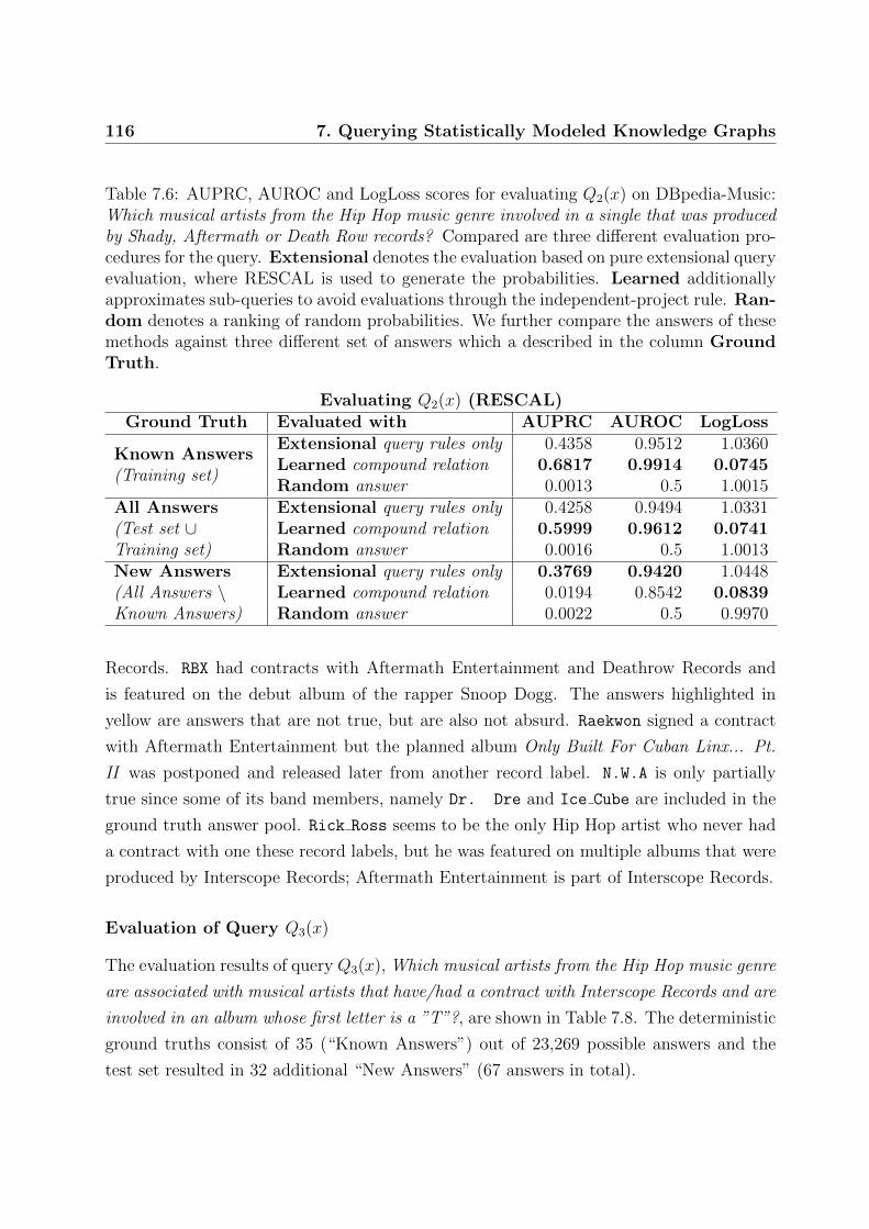
116 7. Querying Statistically Modeled Knowledge Graphs
Table 7.6: AUPRC, AUROC and LogLoss scores for evaluating Q2(x) on DBpedia-Music:Which musical artists from the Hip Hop music genre involved in a single that was producedby Shady, Aftermath or Death Row records? Compared are three different evaluation pro-cedures for the query. Extensional denotes the evaluation based on pure extensional queryevaluation, where RESCAL is used to generate the probabilities. Learned additionallyapproximates sub-queries to avoid evaluations through the independent-project rule. Ran-dom denotes a ranking of random probabilities. We further compare the answers of thesemethods against three different set of answers which a described in the column GroundTruth.
Evaluating Q2(x) (RESCAL)Ground Truth Evaluated with AUPRC AUROC LogLoss
Extensional query rules only 0.4358 0.9512 1.0360Learned compound relation 0.6817 0.9914 0.0745
Known Answers(Training set)
Random answer 0.0013 0.5 1.0015Extensional query rules only 0.4258 0.9494 1.0331Learned compound relation 0.5999 0.9612 0.0741
All Answers(Test set ∪Training set) Random answer 0.0016 0.5 1.0013
Extensional query rules only 0.3769 0.9420 1.0448Learned compound relation 0.0194 0.8542 0.0839
New Answers(All Answers \Known Answers) Random answer 0.0022 0.5 0.9970
Records. RBX had contracts with Aftermath Entertainment and Deathrow Records and
is featured on the debut album of the rapper Snoop Dogg. The answers highlighted in
yellow are answers that are not true, but are also not absurd. Raekwon signed a contract
with Aftermath Entertainment but the planned album Only Built For Cuban Linx... Pt.
II was postponed and released later from another record label. N.W.A is only partially
true since some of its band members, namely Dr. Dre and Ice Cube are included in the
ground truth answer pool. Rick Ross seems to be the only Hip Hop artist who never had
a contract with one these record labels, but he was featured on multiple albums that were
produced by Interscope Records; Aftermath Entertainment is part of Interscope Records.
Evaluation of Query Q3(x)
The evaluation results of query Q3(x), Which musical artists from the Hip Hop music genre
are associated with musical artists that have/had a contract with Interscope Records and are
involved in an album whose first letter is a ”T”?, are shown in Table 7.8. The deterministic
ground truths consist of 35 (“Known Answers”) out of 23,269 possible answers and the
test set resulted in 32 additional “New Answers” (67 answers in total).
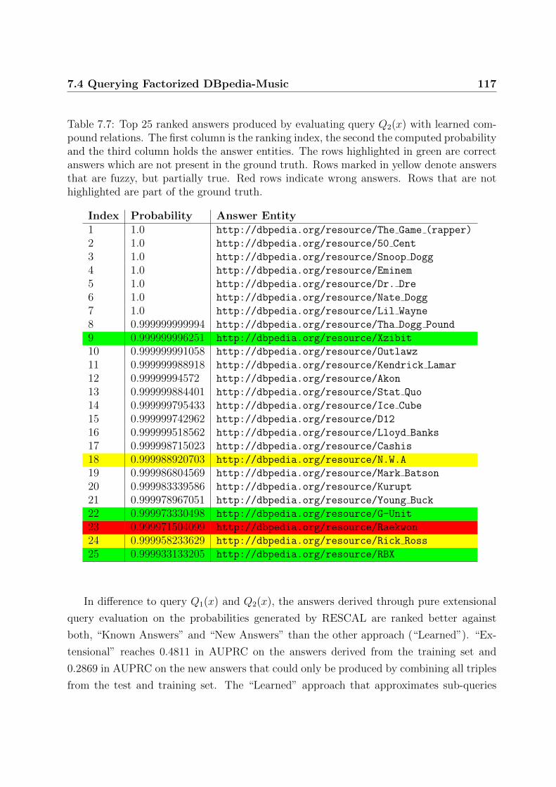
7.4 Querying Factorized DBpedia-Music 117
Table 7.7: Top 25 ranked answers produced by evaluating query Q2(x) with learned com-pound relations. The first column is the ranking index, the second the computed probabilityand the third column holds the answer entities. The rows highlighted in green are correctanswers which are not present in the ground truth. Rows marked in yellow denote answersthat are fuzzy, but partially true. Red rows indicate wrong answers. Rows that are nothighlighted are part of the ground truth.
Index Probability Answer Entity1 1.0 http://dbpedia.org/resource/The Game (rapper)
2 1.0 http://dbpedia.org/resource/50 Cent
3 1.0 http://dbpedia.org/resource/Snoop Dogg
4 1.0 http://dbpedia.org/resource/Eminem
5 1.0 http://dbpedia.org/resource/Dr. Dre
6 1.0 http://dbpedia.org/resource/Nate Dogg
7 1.0 http://dbpedia.org/resource/Lil Wayne
8 0.999999999994 http://dbpedia.org/resource/Tha Dogg Pound
9 0.999999996251 http://dbpedia.org/resource/Xzibit
10 0.999999991058 http://dbpedia.org/resource/Outlawz
11 0.999999988918 http://dbpedia.org/resource/Kendrick Lamar
12 0.99999994572 http://dbpedia.org/resource/Akon
13 0.999999884401 http://dbpedia.org/resource/Stat Quo
14 0.999999795433 http://dbpedia.org/resource/Ice Cube
15 0.999999742962 http://dbpedia.org/resource/D12
16 0.999999518562 http://dbpedia.org/resource/Lloyd Banks
17 0.999998715023 http://dbpedia.org/resource/Cashis
18 0.999988920703 http://dbpedia.org/resource/N.W.A
19 0.999986804569 http://dbpedia.org/resource/Mark Batson
20 0.999983339586 http://dbpedia.org/resource/Kurupt
21 0.999978967051 http://dbpedia.org/resource/Young Buck
22 0.999973330498 http://dbpedia.org/resource/G-Unit
23 0.999971504099 http://dbpedia.org/resource/Raekwon
24 0.999958233629 http://dbpedia.org/resource/Rick Ross
25 0.999933133205 http://dbpedia.org/resource/RBX
In difference to query Q1(x) and Q2(x), the answers derived through pure extensional
query evaluation on the probabilities generated by RESCAL are ranked better against
both, “Known Answers” and “New Answers” than the other approach (“Learned”). “Ex-
tensional” reaches 0.4811 in AUPRC on the answers derived from the training set and
0.2869 in AUPRC on the new answers that could only be produced by combining all triples
from the test and training set. The “Learned” approach that approximates sub-queries
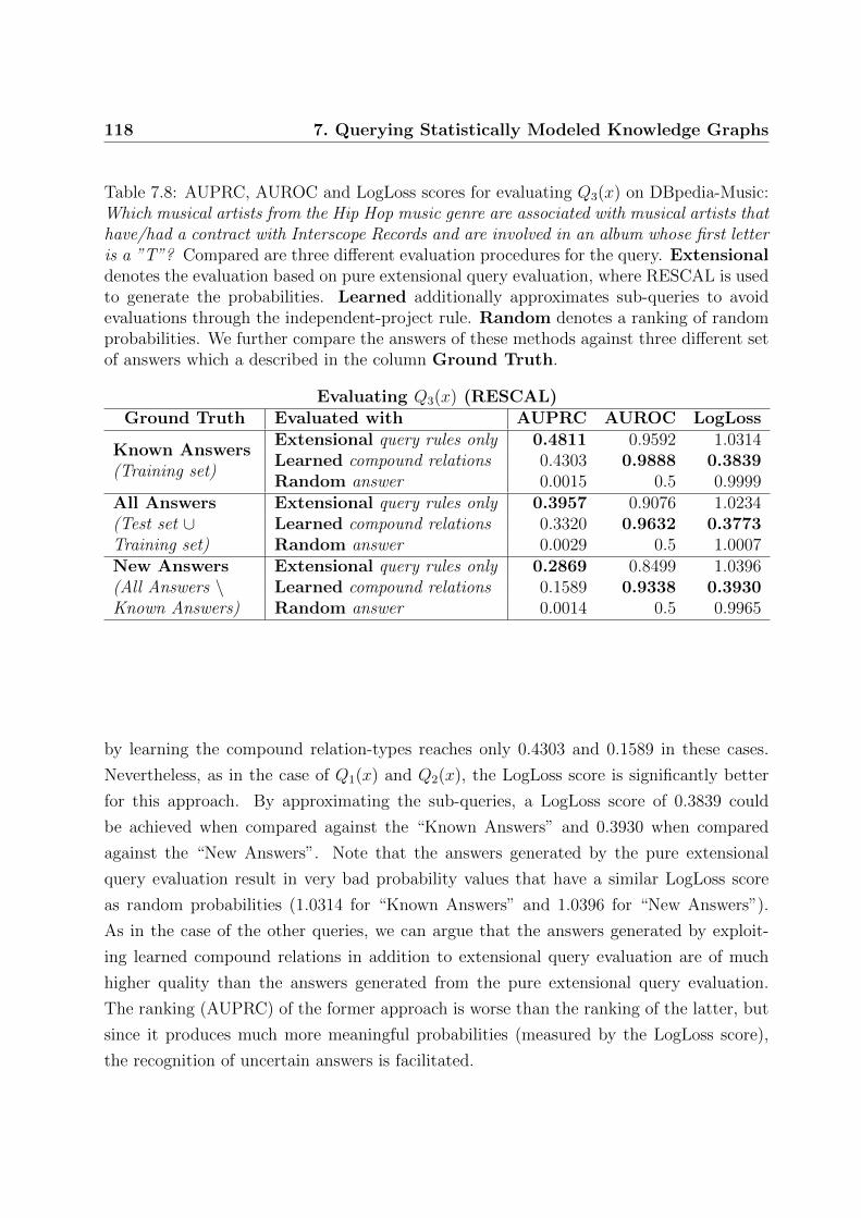
118 7. Querying Statistically Modeled Knowledge Graphs
Table 7.8: AUPRC, AUROC and LogLoss scores for evaluating Q3(x) on DBpedia-Music:Which musical artists from the Hip Hop music genre are associated with musical artists thathave/had a contract with Interscope Records and are involved in an album whose first letteris a ”T”? Compared are three different evaluation procedures for the query. Extensionaldenotes the evaluation based on pure extensional query evaluation, where RESCAL is usedto generate the probabilities. Learned additionally approximates sub-queries to avoidevaluations through the independent-project rule. Random denotes a ranking of randomprobabilities. We further compare the answers of these methods against three different setof answers which a described in the column Ground Truth.
Evaluating Q3(x) (RESCAL)Ground Truth Evaluated with AUPRC AUROC LogLoss
Extensional query rules only 0.4811 0.9592 1.0314Learned compound relations 0.4303 0.9888 0.3839
Known Answers(Training set)
Random answer 0.0015 0.5 0.9999Extensional query rules only 0.3957 0.9076 1.0234Learned compound relations 0.3320 0.9632 0.3773
All Answers(Test set ∪Training set) Random answer 0.0029 0.5 1.0007
Extensional query rules only 0.2869 0.8499 1.0396Learned compound relations 0.1589 0.9338 0.3930
New Answers(All Answers \Known Answers) Random answer 0.0014 0.5 0.9965
by learning the compound relation-types reaches only 0.4303 and 0.1589 in these cases.
Nevertheless, as in the case of Q1(x) and Q2(x), the LogLoss score is significantly better
for this approach. By approximating the sub-queries, a LogLoss score of 0.3839 could
be achieved when compared against the “Known Answers” and 0.3930 when compared
against the “New Answers”. Note that the answers generated by the pure extensional
query evaluation result in very bad probability values that have a similar LogLoss score
as random probabilities (1.0314 for “Known Answers” and 1.0396 for “New Answers”).
As in the case of the other queries, we can argue that the answers generated by exploit-
ing learned compound relations in addition to extensional query evaluation are of much
higher quality than the answers generated from the pure extensional query evaluation.
The ranking (AUPRC) of the former approach is worse than the ranking of the latter, but
since it produces much more meaningful probabilities (measured by the LogLoss score),
the recognition of uncertain answers is facilitated.
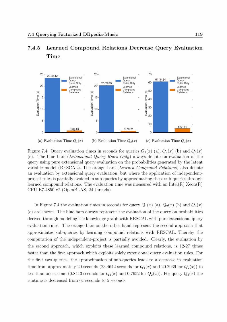
7.4 Querying Factorized DBpedia-Music 119
7.4.5 Learned Compound Relations Decrease Query Evaluation
Time
0
5
10
15
20
25
Evalua
tion Time (s)
23.4642
0.8413
ExtensionalQueryRules OnlyLearnedCompoundRelations
(a) Evaluation Time Q1(x)
0
5
10
15
20
25
Evalua
tion Time (s)
20.2939
0.7652
ExtensionalQueryRules OnlyLearnedCompoundRelations
(b) Evaluation Time Q2(x)
0
10
20
30
40
50
60
70
Evalua
tion Time (s)
61.3424
5.0111
ExtensionalQueryRules OnlyLearnedCompoundRelations
(c) Evaluation Time Q3(x)
Figure 7.4: Query evaluation times in seconds for queries Q1(x) (a), Q2(x) (b) and Q3(x)(c). The blue bars (Extensional Query Rules Only) always denote an evaluation of thequery using pure extensional query evaluation on the probabilities generated by the latentvariable model (RESCAL). The orange bars (Learned Compound Relations) also denotean evaluation by extensional query evaluation, but where the application of independent-project rules is partially avoided in sub-queries by approximating these sub-queries throughlearned compound relations. The evaluation time was measured with an Intel(R) Xeon(R)CPU E7-4850 v2 (OpenBLAS, 24 threads)
In Figure 7.4 the evaluation times in seconds for query Q1(x) (a), Q2(x) (b) and Q3(x)
(c) are shown. The blue bars always represent the evaluation of the query on probabilities
derived through modeling the knowledge graph with RESCAL with pure extensional query
evaluation rules. The orange bars on the other hand represent the second approach that
approximates sub-queries by learning compound relations with RESCAL. Thereby the
computation of the independent-project is partially avoided. Clearly, the evaluation by
the second approach, which exploits these learned compound relations, is 12-27 times
faster than the first approach which exploits solely extensional query evaluation rules. For
the first two queries, the approximation of sub-queries leads to a decrease in evaluation
time from approximately 20 seconds (23.4642 seconds for Q1(x) and 20.2939 for Q2(x)) to
less than one second (0.8413 seconds for Q1(x) and 0.7652 for Q2(x)). For query Q3(x) the
runtime is decreased from 61 seconds to 5 seconds.
120 7. Querying Statistically Modeled Knowledge Graphs
A Comment on the Difference in Evaluation Time of Extensional Query Eval-
uation in Comparison to the Publication “Querying Factorized Probabilistic
Triple Databases”
In [57], we reported much larger evaluation time for query Q3(x) when evaluating this
query solely through extensional query evaluation rules. In fact, we reported that this
query remained unanswered after 6 hours. It might be surprising that we reported in
the previous section that this query is answered by the same evaluation procedure in 61
seconds.
This large difference in evaluation time is caused by different algorithms that were used
to compute the independent-project rule. In [57], we made the restriction that it should
be possible to evaluate the query on commodity hardware. For this reason we avoided
any materialization of whole relation-types leading to a dense (type-constrained) frontal
slice of the tensor. In most of the knowledge graphs there exist relation-types that are
unbounded, meaning that domain or range constraints are defined over owl#Thing. For
large knowledge graphs which contain millions of entities, a materialization of this kind of
relation-types from the learned latent variable model becomes quickly intractable due to
the huge amount of values (probabilities) that are computed (one for each possible triple).
To avoid this explosion in memory we can compute Q3(x) step by step or block-wise, but
this will lead to a significant increase in computation time. In [57], we report the evaluation
times based on this memory saving algorithm.
In the previous section, we discarded this restriction and materialized whole relations
to compute the queries, i.e. the evaluation through independent-project rule, much more
efficiently. It has to be kept in mind that this approach would need a very powerful
computer system for larger knowledge graphs and can even then be intractable. Even
more impressive, the proposed approach, which partially avoids the evaluation through
the independent-project rule by learning compound relations (exploiting intrinsic features
of the a priori learned latent variable model), is still magnitudes (12-17 times) faster in
evaluating the studied queries than the purely rule based evaluation.
7.5 Related Work
Probabilistic databases (PDB) have gained much interest in recent years and an overview
over the state of the art is provided by [100]. Important ongoing research projects include
the MayBMS project [47] at Cornell University, the MystiQ project [13] at the University
7.5 Related Work 121
of Washington, the Orion project [97] at the Purdue University, and the Trio project [75]
at the Stanford University. The idea of materialized views on PDBs has been developed
in [23], where it was proposed to materialize probabilistic views to be used for query
answering at runtime.
Uncertainty in Semantic Web ontologies has been addressed in BayesOWL [24] and
OntoBayes [115]. Furthermore, PR-OWL [21] is a Bayesian Ontology Language for the
Semantic Web. The link between PDBs, Description Logic and Semantic Web data struc-
tures has been explored by [38, 15, 70]. In contrast to these approaches, we start with a
deterministic triple store and then derive probabilities via the factorization. Common to
all these approaches is the challenge of efficient querying.
In this chapter and in [57] we performed a probabilistic ranking of candidate query an-
swers as done by the top-k querying approaches [27, 84, 95]. However, in difference to these
approaches we are pruning low-confidence answers. In these top-k querying approaches,
the computation of exact probabilities for the potential top-k answers are avoided by using
lower and upper bounds for the corresponding marginal probabilities. Unfortunately, none
of these approaches, apart from [27], can avoid extensive materializations in finding answer
candidates [103].
As discussed in Chapter 4.4, tensors and other latent variable models have been applied
to Web analysis, especially in the context of link-prediction. Link-prediction can be seen
as querying a statistically modeled knowledge graph for ground triples. In [83], the YAGO
ontology was factorized and meaningful predictions of simple triples in selected subgroups
of YAGO were derived through the reconstruction from the low rank representation of the
triple store. In this sense, [9, 25, 99] also applied their models for the evaluation of indepen-
dent triples, but never addressed complex querying on the predictions. In this chapter and
[57], we study the significantly more difficult problem of complex querying with predicted
triple confidence values (including existentially quantified variables). In this regard, we re-
alize extensional query evaluation on safe queries which can induce complex dependencies
between individual predicted triple probabilities throughout the database. In particular,
we are concerned with how these queries can be executed efficiently, without the need for
extensive materialization of probability tables, by exploiting the factorized representation
during querying. In difference to [57], we additionally exploit type-constraints of relation-
types when modeling the knowledge graph and during query evaluation. It was shown
in the Chapter 5 and [54, 17, 56] that latent variable models generally benefit to a large
extent from such prior knowledge on relation-types.
122 7. Querying Statistically Modeled Knowledge Graphs
7.6 Conclusion
In this chapter we have demonstrated that knowledge graphs that are statistically modeled
with latent variable models can be interpreted as probabilistic databases and can be queried
by exploiting the probabilities generated by these models. This approach goes clearly be-
yond querying for ground triples which is basically performed when applying these models
for link-prediction. In this context, we focused on safe queries which can be evaluated in
polynomial time by extensional query evaluation rules. We used latent variable models to
represent probabilities for a huge amount of triples very efficiently, since it is intractable to
explicitly represent the probabilities for every possible triple (considering type-constraints)
of the knowledge graph. As a drawback, the probabilities have to be computed “on the
fly” when evaluating the queries, which causes additional computational overhead. This
computational overhead can be especially severe if sub-queries have to be evaluated using
the independent-project rule. We showed that the evaluation of sub-queries through the
independent-project rule can be partially avoided by predicting compound relations from
the initial deterministic knowledge graph with the pre-trained latent variable model. In
our first set of experiments, we gave empirical poof that the evaluation of sub-queries of the
form Q(x, z) : −L1(x, y), L2(y, z), using the extensional query evaluation rules or using the
predicted compound relation L3(x, z), results in a similar ranking of probabilities. We fur-
ther applied both approaches for querying DBpedia-Music, a sub-graph of DBpedia which
contains entities and relation-types that are related to music. From the experimental re-
sult, we can conclude that the approximation of sub-queries through predicted compound
relations has many advantages over the evaluation of the queries with pure extensional
evaluation rules. First, the query evaluation time is reduced by multiple factors, even
when disregarding memory consumption aspects (which lead to faster computations) when
evaluating by the independent-project rule. Furthermore, the learned memory efficient rep-
resentation of the compound relation-types can be stored and used as precomputed views
to further decrease query evaluation time in subsequent queries. Second, it results in signif-
icantly more meaningful probabilities for the derived answers for the various queries. This
observation is particularly interesting, because it allows a more reliable identification of
uncertain answers. Third, the approximation of sub-queries through predicted compound
relations avoids numerical problems when applying the independent-project rule, where a
product of a large number of probabilities has to be computed. In general, the approach
is not restricted to the ∃x.Q type queries, but can always be employed when views can be
used to simplify the probabilistic query.
Chapter 8Conclusion
8.1 Summary
In this work, we have studied the application of latent variable models for the statistical
modeling of large knowledge graphs. The statistical modeling of these graphs plays an
important role in tasks related to completion and cleansing, but also for the automatic
construction of knowledge graphs from unstructured textual data. Due to their size, large
knowledge graphs are especially challenging to model because they introduce additional
constraints on the statistical model, i.e. limiting the complexity of the embedding space
of the latent representations for relation-types and entities. Enforcing large embeddings
to increase the expressiveness of latent variable models will inevitably lead to very long to
intractable training times and high memory consumption when exploiting them for these
graphs. For this reason, it has to be considered that the latent variable models have to be
parsimonious in their number of parameters to be tractable. Examples include Google’s
Knowledge Vault system, where the used neural network exploits latent embedding vectors
of length no more than 60 to model the entities and relation-types of Freebase, which
has millions of entities and thousands of relation-types. Throughout this work, we have
considered three different latent variable models that cover the current state of the art in
scalable latent variable models for the statistical modeling of large knowledge graphs. The
first, RESCAL, is a very efficient third order tensor factorization method which exploits
the natural representation of triples in a third-order tensor. The second, Translational
Embeddings (TransE) model interprets triples as translations in the latent embedding
space, and the third, mwNN is the earlier mentioned multiway neural network approach
used in the Google Knowledge Vault system.
124 8. Conclusion
In our initial experiments presented in Chapter 4, we compared these models under the
constraints imposed by large knowledge graphs. From these experiments, we observed that
the prediction quality of all three models on selected data sets from Freebase, DBpedia and
YAGO was often of moderate quality when these models are limited in their complexity.
TransE clearly achieved the highest prediction quality in the link-prediction tasks when
compared with the other two models, but RESCAL is clearly superior in terms of training
times and it has a low number of hyper-parameters, decreasing model tuning effort to
a minimum. The multiway neural network model (mwNN) resulted in a similar link-
prediction quality than RESCAL, but with significantly longer training times. This model
is also the most complex one in terms of hyper-parameters, resulting in a high effort for
hyper-parameter tuning.
It is intractable to generally increase the dimensionality of the latent embeddings for
entities and relation-types to improve the expressiveness of latent variable models when
modeling large knowledge graphs. For this reason we require a different approach to reduce
the complexity of the modeling tasks that will empower the latent variable models to focus
on the important aspects of the data. We showed in Chapter 5 that prior knowledge
on relation-types in form of type-constraints, as provided by the schema of knowledge
graphs, is one effective way to reduce this complexity with great impact on the modeling
quality. For all three latent variable models and a diverse set of triple data extracted
from Freebase, DBpedia and YAGO, we were able to observe improvements up to 77% in
link-prediction quality in terms of Area Under Precision Recall Curve. Due to the many
aspects in which these models differ and the fact that they have been the major targets
for extensions from multiple research groups around the globe, we further argue that the
observed improvements are not limited to the studied three models (RESCAL, TransE
and mwNN), but that the integration of prior knowledge on relation-types is of general
value to latent variable models when modeling knowledge graphs. In addition, we could
observe similar large improvements when exploiting a local closed-world assumption on
relation-types instead of type-constraints. The great advantage of this local closed-world
assumption lies in the fact that it is independent from any prior knowledge about the
knowledge graph’s schema, but is solely based on observed triples in the graph. We could
not observe from our experiments that the integration of the local closed-world assumption
leads to generally better results than the integration of curated type-constraints into the
latent variable models. For this reason, the local closed-world assumption should be applied
on those relation-types where type-constraints are missing or fuzzy. In difference to type-
8.1 Summary 125
constraints, the local closed-world assumption can also be applied to schema-less knowledge
graphs.
Besides improving models individually, a different way to improve link-prediction is to
combine diverse predictors in ensemble methods. We have provided and discussed empirical
proof in Chapter 6 that due to their large amount of differences, RESCAL, TransE and
mwNN are well suited for combination in an ensemble solution for link-prediction in large
knowledge graphs. In the conducted experiments the ensemble always resulted in superior
prediction quality with improvements of up to 15% on top of the improvements achieved
through the integration of type-constraints in the individual models. Especially TransE was
observed to learn different aspects of the data than RESCAL or mwNN and the combination
of the TransE with the other two models resulted in the largest improvements over the
best single predictor incorporated in the ensemble. These improvements were observed to
be especially large when the models exploited very low dimensional embedding for entities
and relation-types, where the ensemble method achieved a similar performance as the best
single predictor that was allowed to exploit 10 times higher dimensional embeddings.
When applying latent variable models to knowledge graphs for link-prediction, this is
basically a singular event. We model the given deterministic knowledge graph once and
extract the triple confidences which are exploited for complementing or cleaning the triples
in the graphs in a follow up step, and discard the model afterwards. In Chapter 7, we
described a new interpretation of the trained statistical model as probabilistic database
which extends its application beyond predicting confidences for ground triples. This new
interpretation allows us to exploit the theory of probabilistic databases for complex proba-
bilistic querying of these graphs. Since it is intractable to pursue the naive approach, where
we materialize all possible triple probabilities and simply apply probabilistic rules for query
evaluation, we showed that an alternative approach, which recycles the learned latent rep-
resentations of entities and relation-types, makes probabilistic safe querying tractable on
statistically modeled large knowledge graphs. As a drawback, this alternative approach
introduces additional computational load which can lead to significantly increased query
evaluation times, even though the queries are safe and especially if the independent-project-
rule on a large amount of entities is applied. We proposed to learn compound relations
by exploiting intrinsic features of the latent variable model and showed that the learned
compound relations lead to very good approximations of an instead applied independent-
project-rule decreasing the total query evaluation time dramatically (12-27 times faster).
Furthermore, these learned compound relations avoid numerical issues that can arise when
126 8. Conclusion
the independent project rule is applied on a large set of probabilities. In our experiments,
where we queried the music domain of DBpedia, the evaluation approach which combines
extensional query evaluation rules with learned compound relations resulted in clearly more
meaningful probabilities for the produced answers.
8.2 Future Directions and Applications
Knowledge graphs are of great value for a wide set of applications today, but they also
suffer from many deficiencies. Especially incompleteness is one of the major problems in
these graphs that can only be tackled with the support of reliable automated approaches.
For this reason, there is a high demand for statistical models which support in applications
such as knowledge graph construction, completion and cleaning, but also for dealing with
uncertainties. Latent variable models have proven to be well suited for the modeling of
knowledge graphs, but due to the limitations imposed by the size of large knowledge graphs,
we belief that these models have to be combined with prior knowledge on the graph or its
structure to unfold their full potential. The integration of prior knowledge about relation-
types lead to improved low dimensional embeddings of entities and relation-types that
are of interest for tasks related to disambiguation and link-based clustering in large scale
applications.
Furthermore, there are many aspects in which RESCAL, TransE and KVNN differ
(see discussion in Chapter 3.3) and which have to be analyzed more deeply. Identifying
these models’ key aspects that have the most beneficial impact on link-prediction quality
can give rise to a new generation of latent variable approaches that could further drive
knowledge-graph modeling. Nevertheless, we expect that it will be very difficult for the
current state of the art latent variable models to capture the complete underlying structure
and dependencies of the whole knowledge graph under the complexity limits imposed by
large knowledge graphs on the embedding space. The combination of latent variable models
with graph-feature models as proposed by [25, 80] or the combination of diverse models of
low complexity as proposed in this work offer an efficient way to increase link-prediction
quality. Unfortunately, these ensemble methods will not result in better embeddings for
entities or relation-types which are of major interest for various applications that rely on
embeddings reflecting the semantics of entities and relation-types. A possible solution to
this problem is offered by Deep Learning approaches where the complexity of the learning
task can be covered by a hierarchy of neural network layers that result in latent features
8.2 Future Directions and Applications 127
that reflect more complex dependencies observed in the graph. In contrast to the other
latent variable approaches, the deeper layers in the neural network hierarchy are not directly
dependent on the size of the knowledge graph as the first embedding layer and will therefore
not necessarily explode in the amount of parameters. A potential successful application
of Deep Learning for link-prediction in knowledge graphs is currently an open research
question, but very promising.
Additionally, in some cases the truthfulness of a triple might not only be dependent on
single ground triples, as considered by the latent variable models discussed in this work,
but on complex associations of facts that actually represent whole paths in the knowledge
graphs (e.g. nested facts). It might be beneficial to consider these paths in a whole and
not as a composition of independent atomic triples when modeling the knowledge graphs
[77, 40]. Models that are able to additionally consider these paths are of special interest
for querying knowledge graphs and could further complement the probabilistic querying of
knowledge graphs proposed in Chapter 7.

128 8. Conclusion
Bibliography
[1] Dean Allemang and James Hendler. Semantic Web for the Working Ontologist -
Effective Modeling in RDFS and OWL. Morgan Kaufmann/Elsevier, 2nd revised
edition. edition, 2011.
[2] M. Ashburner, C. A. Ball, J. A. Blake, D. Botstein, H. Butler, J. M. Cherry, A. P.
Davis, K. Dolinski, S. S. Dwight, J. T. Eppig, M. A. Harris, D. P. Hill, L. Issel-
Tarver, A. Kasarskis, S. Lewis, J. C. Matese, J. E. Richardson, M. Ringwald, and
G. M. Rubin & G. Sherlock. Gene ontology: tool for the unification of biology.
Nature Genetics, 25:25–29, May 2000.
[3] Brett W. Bader, Richard A. Harshman, and Tamara G. Kolda. Temporal analysis
of semantic graphs using asalsan. 2013 IEEE 13th International Conference on Data
Mining, 0:33–42, 2007.
[4] Yoshua Bengio, Aaron Courville, and Pascal Vincent. Representation learning: A
review and new perspectives. IEEE Trans. Pattern Anal. Mach. Intell., 35(8):1798–
1828, August 2013.
[5] James Bergstra, Olivier Breuleux, Frederic Bastien, Pascal Lamblin, Razvan Pas-
canu, Guillaume Desjardins, Joseph Turian, David Warde-Farley, and Yoshua Ben-
gio. Theano: a CPU and GPU math expression compiler. In Proceedings of the
Python for Scientific Computing Conference (SciPy), June 2010.
[6] C. Bizer, T. Heath, and T. Berners-Lee. Linked data - the story so far. Int. J.
Semantic Web Inf. Syst., 5(3):122, 2009.
130 BIBLIOGRAPHY
[7] Stephan Bloehdorn, Peter Haase, York Sure, and Johanna Vlker. Ontology evolution.
In John Davies, Rudi Studer, and Paul Warren, editors, Semantic Web Technologies
— Trends and Research in Ontology-Based Systems, chapter 4, pages 51–70. John
Wiley & Sons, Chichester, West Sussex, UK, June 2006.
[8] Kurt Bollacker, Colin Evans, Praveen Paritosh, Tim Sturge, and Jamie Taylor. Free-
base: A collaboratively created graph database for structuring human knowledge. In
Proceedings of the 2008 ACM SIGMOD International Conference on Management
of Data, SIGMOD ’08, pages 1247–1250, New York, NY, USA, 2008. ACM.
[9] Antoine Bordes, Nicolas Usunier, Alberto Garcia-Duran, Jason Weston, and Oksana
Yakhnenko. Translating embeddings for modeling multi-relational data. In C.J.C.
Burges, L. Bottou, M. Welling, Z. Ghahramani, and K.Q. Weinberger, editors, Ad-
vances in Neural Information Processing Systems 26, pages 2787–2795. Curran As-
sociates, Inc., 2013.
[10] Antoine Bordes, Nicolas Usunier, Alberto Garcıa-Duran, Jason Weston, and Oksana
Yakhnenko. Translating embeddings for modeling multi-relational data. In Advances
in Neural Information Processing Systems 26: 27th Annual Conference on Neural
Information Processing Systems 2013. Proceedings of a meeting held December 5-8,
2013, Lake Tahoe, Nevada, United States., pages 2787–2795, 2013.
[11] Antoine Bordes, Jason Weston, Ronan Collobert, and Yoshua Bengio. Learning
structured embeddings of knowledge bases. In AAAI, 2011.
[12] Antoine Bordes, Xavier Glorot Jason Weston, and Yoshua Bengio. A semantic match-
ing energy function for learning with multi-relational data. CoRR, abs/1301.3485,
2013.
[13] Jihad Boulos, Nilesh N. Dalvi, Bhushan Mandhani, Shobhit Mathur, Christopher Re,
and Dan Suciu. Mystiq: a system for finding more answers by using probabilities.
In SIGMOD Conference, pages 891–893, 2005.
[14] Paul Buitelaar, Daniel Olejnik, and Michael Sintek. A protg plug-in for ontology
extraction from text based on linguistic analysis. In Proceedings of the 1st European
Semantic Web Symposium (ESWS04), pages 31–44. Springer, 2004.
BIBLIOGRAPHY 131
[15] Andrea Calı, Thomas Lukasiewicz, Livia Predoiu, and Heiner Stuckenschmidt.
Tightly integrated probabilistic description logic programs for representing ontology
mappings. In FoIKS, pages 178–198, 2008.
[16] A. Carlson, J. Betteridge, B. Kisiel, B. Settles, E.R. Hruschka Jr., and T.M. Mitchell.
Toward an architecture for never-ending language learning. In Proceedings of the
Conference on Artificial Intelligence (AAAI), pages 1306–1313. AAAI Press, 2010.
[17] Kai-Wei Chang, Wen-tau Yih, Bishan Yang, and Christopher Meek. Typed tensor
decomposition of knowledge bases for relation extraction. In Proceedings of the 2014
Conference on Empirical Methods in Natural Language Processing (EMNLP), pages
1568–1579. Association for Computational Linguistics, 2014.
[18] Philipp Cimiano, Andreas Hotho, and Steffen Staab. Learning concept hierarchies
from text corpora using formal concept analysis. J. Artif. Int. Res., 24(1):305–339,
August 2005.
[19] Philipp Cimiano and Johanna Volker. Text2onto: A framework for ontology learning
and data-driven change discovery. In Proceedings of the 10th International Conference
on Natural Language Processing and Information Systems, NLDB’05, pages 227–238,
Berlin, Heidelberg, 2005. Springer-Verlag.
[20] World Wide Web Consortium. Rdf schema 1.1, Feb 2014.
[21] Paulo Cesar G. da Costa, Kathryn B. Laskey, and Kenneth J. Laskey. Pr-owl: A
bayesian ontology language for the semantic web. In ISWC-URSW, 2005.
[22] G.E. Dahl, Dong Yu, Li Deng, and A. Acero. Context-dependent pre-trained deep
neural networks for large-vocabulary speech recognition. Audio, Speech, and Lan-
guage Processing, IEEE Transactions on, 20(1):30 –42, jan. 2012.
[23] Nilesh N. Dalvi, Christopher Re, and Dan Suciu. Queries and materialized views on
probabilistic databases. J. Comput. Syst. Sci., 77(3):473–490, 2011.
[24] Zhongli Ding, Yun Peng, and Rong Pan. A bayesian approach to uncertainty mod-
elling in owl ontology. In Proceedings of the International Conference on Advances
in Intelligent Systems - Theory and Applications, 2004.
132 BIBLIOGRAPHY
[25] Xin L. Dong, Evgeniy Gabrilovich, Geremy Heitz, Wilko Horn, Ni Lao, Kevin Mur-
phy, Thomas Strohmann, Shaohua Sun, and Wei Zhang. Knowledge vault: A web-
scale approach to probabilisitic knowledge fusion. In Proceedings of the 20th ACM
SIGKDD international conference on Knowledge discovery and data mining, pages
601–610, 2014.
[26] John Duchi, Elad Hazan, and Yoram Singer. Adaptive subgradient methods for
online learning and stochastic optimization. J. Mach. Learn. Res., 12:2121–2159,
July 2011.
[27] Maximilian Dylla, Iris Miliaraki, and Martin Theobald. Top-k query processing in
probabilistic databases with non-materialized views. Research Report MPI-I-2012-5-
002, Max-Planck-Institut fur Informatik, Stuhlsatzenhausweg 85, 66123 Saarbrucken,
Germany, June 2012.
[28] Dumitru Erhan, Yoshua Bengio, Aaron Courville, Pierre-Antoine Manzagol, Pascal
Vincent, and Samy Bengio. Why does unsupervised pre-training help deep learning?
J. Mach. Learn. Res., 11:625–660, 2010.
[29] Oren Etzioni, Michele Banko, Stephen Soderland, and Daniel S. Weld. Open infor-
mation extraction from the web. Commun. ACM, 51(12):68–74, December 2008.
[30] Oren Etzioni, Anthony Fader, Janara Christensen, Stephen Soderland, and Mausam
Mausam. Open information extraction: The second generation. In Proceedings of
the Twenty-Second International Joint Conference on Artificial Intelligence - Volume
Volume One, IJCAI’11, pages 3–10. AAAI Press, 2011.
[31] Jerome Euzenat and Pavel Shvaiko. Ontology Matching. Springer-Verlag New York,
Inc., Secaucus, NJ, USA, 2007.
[32] Nicola Fanizzi, Claudia d’Amato, and Floriana Esposito. Dl-foil concept learning in
description logics. In Filip Zelezn and Nada Lavrac, editors, ILP, volume 5194 of
Lecture Notes in Computer Science, pages 107–121. Springer, 2008.
[33] Christiane Fellbaum, editor. WordNet: an electronic lexical database. MIT Press,
1998.
[34] D. A. Ferrucci. Introduction to ”this is watson”. IBM J. Res. Dev., 56(3):235–249,
May 2012.
BIBLIOGRAPHY 133
[35] Thomas Franz, Antje Schultz, Sergej Sizov, and Steffen Staab. Triplerank: Rank-
ing semantic web data by tensor decomposition. In International Semantic Web
Conference, pages 213–228, 2009.
[36] Alberto Garcia-Duran, Antoine Bordes, Nicolas Usunier, and Yves Grandvalet. Com-
bining two and three-way embeddings models for link prediction in knowledge bases.
In arXiv:1506.00999, 2015.
[37] J. Giles. Special Report: Internet encyclopaedias go head to head. Nature, 438, 2005.
[38] Rosalba Giugno and Thomas Lukasiewicz. P-shoq(d): A probabilistic extension of
shoq(d) for probabilistic ontologies in the semantic web. In JELIA, 2002.
[39] Marko Grobelnik and Dunja Mladeni. Knowledge Discovery for Ontology Construc-
tion, pages 9–27. John Wiley & Sons, Ltd, 2006.
[40] Kelvin Gu, John Miller, and Percy Liang. Traversing knowledge graphs in vector
space. CoRR, abs/1506.01094, 2015.
[41] R. A. Harshman. Foundations of the PARAFAC procedure: Models and conditions
for an” explanatory” multi-modal factor analysis. UCLA Working Papers in Pho-
netics, 16(1):84, 1970.
[42] Richard A. Harshman. Parafac2: Mathematical and technical notes. UCLA working
papers in phonetics, 22:30–47, 1972.
[43] Mohammad Al Hasan, Vineet Chaoji, Saeed Salem, and Mohammed Zaki. Link
prediction using supervised learning. In In Proc. of SDM 06 workshop on Link
Analysis, Counterterrorism and Security, 2006.
[44] John Hebeler, Matthew Fisher, Ryan Blace, Andrew Perez-Lopez, and Mike Dean.
Semantic Web Programming -. Wiley, New York, 1. auflage edition, 2009.
[45] G E Hinton and R R Salakhutdinov. Reducing the dimensionality of data with neural
networks. Science, 313(5786):504–507, 2006.
[46] Johannes Hoffart, Fabian M. Suchanek, Klaus Berberich, Edwin Lewis-Kelham, Ger-
ard de Melo, and Gerhard Weikum. Yago2: Exploring and querying world knowledge
in time, space, context, and many languages. In Proceedings of the 20th International
134 BIBLIOGRAPHY
Conference Companion on World Wide Web, WWW ’11, pages 229–232, New York,
NY, USA, 2011. ACM.
[47] Jiewen Huang, Lyublena Antova, Christoph Koch, and Dan Olteanu. Maybms: a
probabilistic database management system. In SIGMOD Conference, 2009.
[48] Tuyen N. Huynh and Raymond J. Mooney. Online structure learning for markov logic
networks. In Machine Learning and Knowledge Discovery in Databases - European
Conference, ECML PKDD 2011, Athens, Greece, September 5-9, 2011, Proceedings,
Part II, pages 81–96, 2011.
[49] Luigi Iannone, Ignazio Palmisano, and Nicola Fanizzi. An algorithm based on coun-
terfactuals for concept learning in the semantic web. Appl. Intell., 26(2):139–159,
2007.
[50] Rodolphe Jenatton, Nicolas Le Roux, Antoine Bordes, and Guillaume Obozinski. A
latent factor model for highly multi-relational data. In NIPS, pages 3176–3184, 2012.
[51] I.T. Jolliffe. Principal Component Analysis. Springer Verlag, 1986.
[52] Tamara G. Kolda, Brett W. Bader, and Joseph P. Kenny. Higher-order web link
analysis using multilinear algebra. In ICDM, pages 242–249, 2005.
[53] Alex Krizhevsky, Ilya Sutskever, and Geoffrey E. Hinton. Imagenet classification
with deep convolutional neural networks. In F. Pereira, C.J.C. Burges, L. Bottou,
and K.Q. Weinberger, editors, Advances in Neural Information Processing Systems
25, pages 1097–1105. Curran Associates, Inc., 2012.
[54] Denis Krompaß, Stephan Baier, and Volker Tresp. Type-constrained representation
learning in knowledge graphs. In Proceedings of the 13th International Semantic Web
Conference (ISWC), 2015.
[55] Denis Krompaß, Maximilian Nickel, Xueyan Jiang, and Volker Tresp. Non-negative
tensor factorization with rescal. In ECML/PKDD 2013 Workshop on Tensor Methods
for Machine Learning, 2013.
[56] Denis Krompaß, Maximilian Nickel, and Volker Tresp. Large-scale factorization of
type-constrained multi-relational data. In Proceedings of the 2014 Conference on
Data Science and Advanced Analytics, 2014.
BIBLIOGRAPHY 135
[57] Denis Krompaß, Maximilian Nickel, and Volker Tresp. Querying factorized prob-
abilistic triple databases. In Proceedings of the 13th International Semantic Web
Conference (ISWC), 2014.
[58] Denis Krompaßand Volker Tresp. Ensemble solutions for link-prediction in knowl-
edge graphs. In Proceedings of the 2nd Workshop on Linked Data for Knowledge
Discovery co-located with European Conference on Machine Learning and Principles
and Practice of Knowledge Discovery in Databases (ECML PKDD 2015), 2015.
[59] Amy N. Langville, Carl D. Meyer, and Russell Albright. Initializations for the non-
negative matrix factorization, 2006.
[60] Ni Lao, Tom Mitchell, and William W. Cohen. Random walk inference and learning
in a large scale knowledge base. In Proceedings of the Conference on Empirical
Methods in Natural Language Processing, EMNLP ’11, pages 529–539, 2011.
[61] Ora Lassila, Ralph R. Swick, World Wide, and Web Consortium. Resource descrip-
tion framework (rdf) model and syntax specification, 1998.
[62] Alan J. Laub. Matrix analysis - for scientists and engineers. SIAM, 2005.
[63] Daniel D. Lee and H. Sebastian Seung. Algorithms for non-negative matrix factor-
ization. In NIPS, pages 556–562, 2000.
[64] Jens Lehmann. Dl-learner: Learning concepts in description logics. J. Mach. Learn.
Res., 10:2639–2642, December 2009.
[65] Jens Lehmann and Pascal Hitzler. A refinement operator based learning algorithm
for the ALC description logic. In Inductive Logic Programming, 17th International
Conference, ILP 2007, Corvallis, OR, USA, June 19-21, 2007, volume 4894 of Lec-
ture Notes in Computer Science, pages 147–160. Springer, 2008.
[66] Jens Lehmann, Robert Isele, Max Jakob, Anja Jentzsch, Dimitris Kontokostas,
Pablo N. Mendes, Sebastian Hellmann, Mohamed Morsey, Patrick van Kleef, Soren
Auer, and Christian Bizer. DBpedia - a large-scale, multilingual knowledge base
extracted from wikipedia. Semantic Web Journal, 2014.
[67] Yankai Lin, Zhiyuan Liu, Maosong Sun, Yang Liu, and Xuan Zhu. Learning entity
and relation embeddings for knowledge graph completion. In AAAI, 2015.
136 BIBLIOGRAPHY
[68] Francesca A. Lisi and Floriana Esposito. An ILP perspective on the semantic web. In
SWAP 2005 - Semantic Web Applications and Perspectives, Proceedings of the 2nd
Italian Semantic Web Workshop, University of Trento, Trento, Italy, 14-16 December
2005, 2005.
[69] Ben London, Theodoros Rekatsinas, Bert Huang, and Lise Getoor. Multi-
relational learning using weighted tensor decomposition with modular loss. CoRR,
abs/1303.1733, 2013.
[70] Thomas Lukasiewicz. Expressive probabilistic description logics. Artif. Intell., 172(6-
7):852–883, 2008.
[71] Alexander Maedche and Steffen Staab. Ontology learning. In HANDBOOK ON
ONTOLOGIES, pages 173–189. Springer, 2004.
[72] Tomas Mikolov, Anoop Deoras, Stefan Kombrink, Luks Burget, and Jan Cernock.
Empirical evaluation and combination of advanced language modeling techniques. In
INTERSPEECH, pages 605–608. ISCA, 2011.
[73] Tomas Mikolov, Ilya Sutskever, Kai Chen, Greg S Corrado, and Jeff Dean. Dis-
tributed representations of words and phrases and their compositionality. In C.J.C.
Burges, L. Bottou, M. Welling, Z. Ghahramani, and K.Q. Weinberger, editors, Ad-
vances in Neural Information Processing Systems 26, pages 3111–3119. Curran As-
sociates, Inc., 2013.
[74] Tomas Mikolov, Wen-tau Yih, and Geoffrey Zweig. Linguistic regularities in con-
tinuous space word representations. In Proceedings of the 2013 Conference of the
North American Chapter of the Association for Computational Linguistics: Human
Language Technologies, pages 746–751, Atlanta, Georgia, June 2013. Association for
Computational Linguistics.
[75] Michi Mutsuzaki, Martin Theobald, Ander de Keijzer, Jennifer Widom, Parag
Agrawal, Omar Benjelloun, Anish Das Sarma, Raghotham Murthy, and Tomoe Sug-
ihara. Trio-one: Layering uncertainty and lineage on a conventional dbms (demo).
In CIDR, pages 269–274, 2007.
[76] Morten Mrup. Applications of tensor (multiway array) factorizations and decomposi-
tions in data mining. Wiley Interdisc. Rew.: Data Mining and Knowledge Discovery,
1(1):24–40, 2011.
BIBLIOGRAPHY 137
[77] Arvind Neelakantan, Benjamin Roth, and Andrew McCallum. Compositional vector
space models for knowledge base completion. CoRR, abs/1504.06662, 2015.
[78] Maximilian Nickel. Tensor factorization for relational learning. PhDThesis, Ludwig-
Maximilian-University of Munich, August 2013.
[79] Maximilian Nickel, Xueyan Jiang, and Volker Tresp. Reducing the rank in rela-
tional factorization models by including observable patterns. In Advances in Neural
Information Processing Systems 27, pages 1179–1187. Curran Associates, Inc., 2014.
[80] Maximilian Nickel, Kevin Murphy, Volker Tresp, and Evgeniy Gabrilovich. A re-
view of relational machine learning for knowledge graphs: From multi-relational link
prediction to automated knowledge graph construction. In arXiv:1503.00759, 2015.
[81] Maximilian Nickel and Volker Tresp. Logistic tensor factorization for multi-relational
data. In Structured Learning: Inferring Graphs from Structured and Unstructured
Inputs (ICML WS), 2013.
[82] Maximilian Nickel, Volker Tresp, and Hans-Peter Kriegel. A three-way model for
collective learning on multi-relational data. In ICML, pages 809–816, 2011.
[83] Maximilian Nickel, Volker Tresp, and Hans-Peter Kriegel. Factorizing yago: scalable
machine learning for linked data. In WWW, pages 271–280, 2012.
[84] Dan Olteanu and Hongkai Wen. Ranking query answers in probabilistic databases:
Complexity and efficient algorithms. In ICDE, pages 282–293, 2012.
[85] W3C OWL Working Group. OWL 2 Web Ontology Language: Document Overview.
W3C Recommendation, 27 October 2009. Available at http://www.w3.org/TR/
owl2-overview/.
[86] Jeffrey Pennington, Richard Socher, and Christopher D. Manning. Glove: Global
vectors for word representation. In Proceedings of the 2014 Conference on Empirical
Methods in Natural Language Processing, EMNLP 2014, October 25-29, 2014, Doha,
Qatar, A meeting of SIGDAT, a Special Interest Group of the ACL, pages 1532–1543,
2014.
[87] John C. Platt. Probabilistic outputs for support vector machines and comparisons to
regularized likelihood methods. In Advances in large margin classifiers, pages 61–74.
MIT Press, 1999.
138 BIBLIOGRAPHY
[88] Hoifung Poon and Pedro Domingos. Unsupervised ontology induction from text.
In Proceedings of the 48th Annual Meeting of the Association for Computational
Linguistics, ACL ’10, pages 296–305, Stroudsburg, PA, USA, 2010. Association for
Computational Linguistics.
[89] Steffen Rendle. Factorization machines. In Proceedings of the 10th IEEE Interna-
tional Conference on Data Mining. IEEE Computer Society, 2010.
[90] Steffen Rendle, Leandro Balby Marinho, Alexandros Nanopoulos, and Lars Schmidt-
Thieme. Learning optimal ranking with tensor factorization for tag recommendation.
In KDD, pages 727–736, 2009.
[91] Achim Rettinger, Uta Losch, Volker Tresp, Claudia D’Amato, and Nicola Fanizzi.
Mining the semantic web. Data Min. Knowl. Discov., 24(3):613–662, May 2012.
[92] Matthew Richardson and Pedro Domingos. Markov logic networks. Machine Learn-
ing, 62(1-2):107–136, 2006.
[93] Richard H. Richens. Preprogramming for mechanical translation. Mechanical Trans-
lation, 1:20–25, 1956.
[94] Sebastian Riedel, Limin Yao, Andrew McCallum, and Benjamin M. Marlin. Relation
extraction with matrix factorization and universal schemas. In HLT-NAACL, pages
74–84, 2013.
[95] Christopher R, Nilesh Dalvi, and Dan Suciu. Efficient top-k query evaluation on
probabilistic data. In in ICDE, pages 886–895, 2007.
[96] Kunal Sengupta, Adila Alfa Krisnadhi, and Pascal Hitzler. Local closed world se-
mantics: Grounded circumscription for owl. In Proceedings of the 10th International
Conference on The Semantic Web - Volume Part I, ISWC’11, pages 617–632, Berlin,
Heidelberg, 2011. Springer-Verlag.
[97] Sarvjeet Singh, Chris Mayfield, Sagar Mittal, Sunil Prabhakar, Susanne E. Hambr-
usch, and Rahul Shah. Orion 2.0: native support for uncertain data. In SIGMOD
Conference, pages 1239–1242, 2008.
[98] Amit Singhal. Introducing the knowledge graph: things, not strings, May 2012.
BIBLIOGRAPHY 139
[99] Richard Socher, Danqi Chen, Christopher D. Manning, and Andrew Y. Ng. Rea-
soning with neural tensor networks for knowledge base completion. In NIPS, pages
926–934, 2013.
[100] Dan Suciu, Dan Olteanu, Christopher Re, and Christoph Koch. Probabilistic
Databases. Synthesis Lectures on Data Management. Morgan & Claypool Publishers,
2011.
[101] Bongwon Suh, Gregorio Convertino, Ed H. Chi, and Peter Pirolli. The singularity
is not near: slowing growth of wikipedia. In WikiSym ’09: Proceedings of the 5th
International Symposium on Wikis and Open Collaboration, pages 1–10, New York,
NY, USA, 2009. ACM.
[102] Chun How Tan, Eugene Agichtein, Panos Ipeirotis, and Evgeniy Gabrilovich. Trust,
but verify: Predicting contribution quality for knowledge base construction and cu-
ration. In WSDM, 2014.
[103] Martin Theobald, Luc De Raedt, Maximilian Dylla, Angelika Kimmig, and Iris Mil-
iaraki. 10 years of probabilistic querying - what next? In ADBIS, 2013.
[104] Volker Tresp, Yi Huang, Markus Bundschus, and Achim Rettinger. Materializing
and querying learned knowledge. In First ESWC Workshop on Inductive Reasoning
and Machine Learning on the Semantic Web (IRMLeS 2009), 2009.
[105] Ledyard R. Tucker. Some mathematical notes on three-mode factor analysis. Psy-
chometrika, 31:279–311, 1966.
[106] Matthew Turk and Alex Pentland. Eigenfaces for recognition. J. Cognitive Neuro-
science, 3(1):71–86, January 1991.
[107] M. Alex O. Vasilescu and Demetri Terzopoulos. Multilinear analysis of image ensem-
bles: Tensorfaces. In IN PROCEEDINGS OF THE EUROPEAN CONFERENCE
ON COMPUTER VISION, pages 447–460, 2002.
[108] Paola Velardi, Roberto Navigli, Alessandro Cucchiarelli, and Francesca Neri. Evalua-
tion of OntoLearn, a methodology for automatic population of domain ontologies. In
Paul Buitelaar, Philipp Cimiano, and Bernardo Magnini, editors, Ontology Learning
from Text: Methods, Applications and Evaluation. IOS Press, 2006.
140 BIBLIOGRAPHY
[109] Brittany Vincent. Siri vs. cortana vs. google now: Why apples siri is best, 2015.
[110] Denny Vrandecic. Wikidata: A new platform for collaborative data collection. In
Proceedings of the 21st International Conference Companion on World Wide Web,
WWW ’12 Companion, pages 1063–1064, New York, NY, USA, 2012. ACM.
[111] Li Wan, Matthew D. Zeiler, Sixin Zhang, Yann LeCun, and Rob Fergus. Regular-
ization of neural networks using dropconnect. In ICML (3), volume 28 of JMLR
Proceedings, pages 1058–1066. JMLR.org, 2013.
[112] Zhen Wang, Jianwen Zhang, Jianlin Feng, and Zheng Chen. Knowledge graph em-
bedding by translating on hyperplanes. In AAAI, July 2014.
[113] Hendrik Wermser, Achim Rettinger, and Volker Tresp. Modeling and learning
context-aware recommendation scenarios using tensor decomposition. In ASONAM,
pages 137–144, 2011.
[114] Bishan Yang, Wen-tau Yih, Xiaodong He, Jianfeng Gao, and Li Deng. Embeddings
entities and relations for learning and inference in knowledge bases. In In ICLR-2015,
2015.
[115] Yi Yang and Jacques Calmet. Ontobayes: An ontology-driven uncertainty model. In
CIMCA/IAWTIC, pages 457–463, 2005.