exploring the use of item bank information to improve irt
TRANSCRIPT

Using Item Bank Information
Exploring the Use of Item Bank Information to Improve IRT Item Parameter Estimation
Erika Hall, Pearson
Timothy Ansley, University of Iowa
On occasion, the sample of students available for calibrating a set of assessment items
may not be optimal. The sample may be small, unrepresentative, or even unmotivated, as
is often the case when there are no direct consequences associated with performance
(e.g., pilot or field-test administration). Each of these situations can be problematic
within the context of Item Response Theory (IRT). For example, it has been
demonstrated repeatedly that the accuracy and stability of IRT item parameter estimates
decreases and root mean squared error (RMSE) and bias increase when small samples are
used for calibration (e.g., Birnbaum, 1968; Swaminathan & Gifford, 1986; Swaminathan,
Hambleton, Sireci, Xing & Rizavi, 2003). Small sample sizes are common in practice
and may occur intentionally, as a means of reducing costs or limiting the exposure of
newly developed items (e.g., CAT); or unintentionally, as the result of a voluntary
sampling plan or an unforeseen administration issue (e.g., a snowstorm on the day the test
is administered). Frequently, small N-counts are the direct result of unavoidable test
design and administration features, as is the case when a relatively large number of forms
must be administered to adequately field test a large pool of newly developed items.
Samples that do not represent the population may produce inappropriate
parameter estimates by restricting the range of ability used for estimation. Research has
shown that accurate item parameter estimation requires the use of a heterogeneous
sample of students that adequately represents the range of abilities measured by the test
(Hambleton, 1993). This requirement is a direct result of working in a regression setting.
1
Using Item Bank Information
In IRT, the conditional probability of a correct response on a given item is displayed by
an item characteristic curve (ICC), the form of which is specified by a given
mathematical model and defined by estimated parameters. For a given item, this curve is
used to represent the regression of item score on student ability and remains the same
regardless of the population of students administered the item. Since the ICC is intended
to accurately represent item performance for the entire test-taking population, the entire
range of abilities underlying this population must be represented in the initial item
calibration. If the appropriate amount and range of information is not available, the true
shape of the ICC may not be realized. Resulting parameter estimates will not display
group-invariance properties or accurately represent the performance of the item for the
total population of interest.
Most research in the IRT literature suggests that Bayesian estimates of item
parameters are more accurate, reasonable, and consistent than maximum likelihood
estimates especially when sample sizes are small and the two- or three-parameter logistic
model is employed (e.g., Gao & Chen, 2005; Swaminathan & Gifford, 1982, 1985, 1986;
Mislevy, 1986; Lord, 1986). Under these conditions, therefore, the question is not
whether Bayesian procedures should be used, but how to specify prior distributions so
that the most accurate item parameter estimates are obtained. To this end, researchers
have explored incorporating collateral information about examinees and items into the
parameter estimation process through the specification of more precise priors. In this
context, collateral information is any information that serves to describe the
characteristics of items or examinees, such as examinee group membership, cognitive
2
Using Item Bank Information
item features (i.e., processes required to answer an item correctly), or estimates of item
difficulty.
The theory behind the use of collateral information to support the specification of
priors is simple. Suppose a probability density function, f(a), is known for a given
parameter, a (e.g., item discrimination). If this is the only information available about a,
the best guess for the value of a would be E(a) = or the mean of the
distribution of a. If a collateral variable k (e.g., content classification) is shown to be
correlated with parameter a, knowledge about the value of k improves the prediction of a
beyond that afforded by its expected value. Therefore, the conditional probability
distribution g(a|k) provides more accurate information about the likely range of values for
parameter a than the unconditional distribution f(a). The stronger the relationship
between a and k, the less variable the conditional distribution, and the greater the
information about the likely value of the parameter. If several collateral variables
improve the prediction of parameter a beyond the use of k alone (as reflected in the
multiple correlation), the conditional distribution of the parameter given all of these
variables should improve estimation even further.
daaaf∫∞
∞−
)(
Use of Collateral Information in Practice
Research on the inclusion of auxiliary information in the estimation process has
produced extremely promising results, even suggesting that if the right information is
available (i.e., collateral variables that are highly correlated to an item’s operating
characteristics), reasonable item parameter estimates can be predicted before or in lieu of
3
Using Item Bank Information
pre-testing; that is, in the absence of student response data (Mislevy, Sheehan, &
Wingersky, 1993).
Given such favorable results, one would think that including such information in
the IRT parameter estimation process would be standard practice. However, for several
reasons this does not appear to be the case. For one, the conditions under which
procedures that incorporate collateral information provide gains over standard marginal
maximum likelihood (MML) or Bayesian estimation procedures are not clear. For
example, while research suggests the application of a data-informed prior improves
estimation when samples are small, very little work has been done concerning the
benefits of exploiting collateral information in the specification of unique item-level prior
distributions, especially within the context of the three-parameter logistic (3-pl) model.
Most research up to this point has focused on the specification of common priors for
these parameters (independent of collateral information), or on the item-level
specification of priors for b-parameters only, with varied results (Gifford &
Swaminathan, 1990; Swaminathan, et. al., 2003). The effectiveness of a procedure that
defines item-level priors for all parameters and all items remains to be explored.
A second possible explanation for the limited use of collateral information in
practice is lack of accessibility to the procedures required to implement the required
estimation techniques correctly and efficiently. Straightforward, user-friendly procedures
(that make use well-defined statistical processes within readily obtainable commercial
software) need to be delineated for identifying “useful” collateral information, specifying
item level priors, and incorporating these priors into the estimation process. In this way,
such procedures will be more likely utilized in practice.
4

Using Item Bank Information
A final reason for the limited use of these procedures is that the available research
provides little information as to how, or if, different types of collateral information
provide different degrees of improvement. Many possible sources of collateral item
information have been proposed (e.g., judges, cognitive item features, test specification
classifications, item forms); however, the extent of gains in estimation accuracy using
each of these sources has not been addressed with a single dataset. Previous research, for
instance, has demonstrated that more precise parameter estimates can be obtained from
small samples when information about items’ cognitive features is incorporated into the
estimation process (Mislevy, 1988), or when content specialists are used to inform the
specification of priors (Swaminathan, Hambleton, Sireci, Xing, & Rizavi, 2003). The
contribution of less expensive, more “readily available” types of information, of the type
typically found in an item bank, has not been addressed. One would expect information
about an item’s cognitive requirements, if accurately classified, to support parameter
estimation better than more general information such as content classification or key,
since the former is more likely correlated with the operating characteristics of the item.
However, a panel of experts is typically required to define these features and classify
each item accordingly—a time consuming and expensive task. General content and
administration data, on the other hand, are available without additional cost.
The goal of the current research was to explore the benefits of incorporating
different types (and combinations) of collateral information into the item parameter
estimation process given samples that vary in size and representativeness, and using
procedures that are relatively straightforward given commercially available software. Of
specific interest was the extent to which readily available information, of the type
5
Using Item Bank Information
typically found in an item bank, might provide for reasonable and effective item
parameter prior distributions. For an English Language Arts assessment for example, this
would include information such as: item sequence and key; associated passage type,
length and readability, and item content classification (e.g., vocabulary, comprehension,
etc). In the current study, the influence of such readily available information on
estimation accuracy and precision was considered independently, and compared with
gains obtained when traditional maximum likelihood and Bayesian procedures were
applied, and with gains obtained when expert judgments regarding item operating
characteristics were considered.
Methodology
Data Two different types of data were used in support of this research: scored student
response data from the census administration of an English Language Arts (ELA)
assessment, and historical item-level data from the item bank from which the items
associated with this assessment were selected. The student response data were the result
of a 64 item, multiple choice, criterion-referenced assessment (ELA CRT) administered
to all eligible seventh grade students in a moderately populated southwestern state. Of the
approximately 33,000 students tested, 83% and 12% reported their ethnicity as White and
Hispanic, respectively. The remaining 5% were Asian, African American, Pacific
Islander or Native American.
The associated grade 7 ELA item bank provided item-level data from one
embedded field-test and two operational administrations for a total of 183 unique items.
The item bank is a repository for all information associated with the given administration
of an item. This information can be organized into four different categories:
6
Using Item Bank Information
administrative (item sequence, session, key); content-related (standard and objective);
passage-related (passage type, length, and difficulty); and performance-related (p-value,
point biserial, IRT parameters, item fit). The first three categories of information are
determined during item and/or test development. They will therefore be referred
throughout this document as “readily available”. That is, no additional work is required
beyond that typically done during item and test development to obtain this information
for use in the specification of prior distributions.
Generation of Research Samples
To determine how the characteristics of the calibration sample interact with the
estimation technique, 12 samples, varying both in size and in the extent to which they
represented the total examinee population with respect to ethnicity, were selected from
the population dataset. Based on previous research on Bayes estimation of item
parameters, and the decision to use the three-parameter model, sample sizes of 100, 200,
500, and 1,000 were selected for use. Samples of each size were nested in three ethnic-
representation categories that varied in terms of their degree of alignment to the
population as a whole: representative, unrepresentative, and extremely unrepresentative.
Given the extremely small number of Asian, African American, Native American and
Pacific Islander examinees, students were classified as either Hispanic or Non-Hispanic.
This simplified both the sample generation process and the interpretation of results.
To generate the representative samples, students were selected at random from the
total population so that the proportions of Hispanic and Non-Hispanic examinees in each
sample mirrored those in the total population (i.e., 12% and 88%, respectively).
7

Using Item Bank Information
Unrepresentative and extremely unrepresentative samples consisted of 50% and 90%
Hispanic students, respectively.
Estimation of “Baseline” Population Item Parameters
To examine the differential impact of sample characteristics and collateral
information on estimation accuracy, item parameters were estimated under a variety of
conditions. Each set of estimated parameters was subsequently compared to a set of
“baseline” parameters. In this case, the baseline item parameters against which all
estimated values were compared were those previously estimated using all grade 7
students who participated in the census administration of the ELA assessment. Baseline
parameters were estimated using BILOG-MG under the assumptions of a three-parameter
logistic item response theory (IRT) model. For this assessment, a normal distribution was
assumed for ability and a common Beta prior was applied to all c-parameters. Priors
were not applied in the estimation of item difficulty or item discrimination.
Parameter Estimation Conditions
For each of the twelve samples previously defined, item parameter estimates were
generated under several conditions which differed in terms of how (and/or if) collateral
information was integrated into the parameter estimation process. The defining
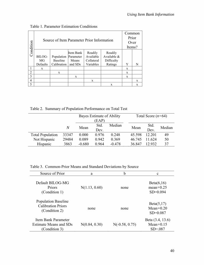
characteristics of each of these conditions are outlined in Table 1.
-------------------------------- Insert Table 1.
-------------------------------- The first column of this table provides the condition to which the remaining columns
refer. The next five columns indicate the source of the information used in specifying
item parameter prior means. Columns 7 and 8 indicate whether applied item parameter
8
Using Item Bank Information
prior distributions were common across items (Y) or uniquely determined for each item
(N).
In the first condition, Bayes estimates of item parameters were generated using
BILOG-MG’s default item parameter prior specifications. For the three-parameter
model, this is a lognormal prior for the a-parameter with a mean of 0 and a standard
deviation of 0.5; and a Beta prior for the c-parameter with ALPHA and BETA set to 6
and 16, respectively. Condition 1 emulates the specifications typically applied in practice
when estimating item parameters under the three-parameter model; collateral information
is ignored, but the importance of assigning a prior distribution to the a- and c-parameters
is acknowledged.
In the second condition, the estimation rules applied in the generation of the
“baseline” parameters were utilized (i.e., no priors for a and b, and a BETA prior with
parameters of ALPHA=5 and BETA=17 for c). Using the same estimation specifications
applied during the population calibration allowed for the effect of sample size and
representativeness on estimation accuracy to be considered independent of estimation
technique.
In BILOG-MG, specific types of prior distributions are required for each
parameter: lognormal for a-parameters; normal for b-parameters, and beta for c-
parameters. For Condition 3, all of the unique items in the Grade 7 ELA item bank were
initially used to generate distributions of log of a-parameters, b-parameters, and c-
parameters. These distributions were subsequently reviewed for extreme values, or
outliers, so that inappropriate values could be removed before analysis. Finally, the
moments of each distribution were used to specify the parameters of the a-, b-, and c-
9
Using Item Bank Information
prior distributions. One prior distribution was specified for each type of parameter, and
then applied to all items.
The ALPHA and BETA parameters used to specify the common Beta prior
distribution for c were calculated using the mean of the c-parameter estimates in the item
bank and the equations for ALPHA and BETA provided in the BILOG-MG user’s
manual (Zimowski, et. al., 2003): ALPHA=mp+1 and BETA= m(1-p)+1. In this
equation p is the expected mean of the distribution, and m is a priori weight that defines
one’s confidence in the prior information. Initially, the BILOG-MG default value of
m=20 was specified in the calculation of ALPHA and BETA. The reasonableness of
these parameters was then assessed by identifying the resulting credibility interval around
c (using the tables in Novick & Jackson, 1974, p. 402), and determining how well it
reflected the distribution of c-parameter estimates in the item bank.
In Condition 4 multiple regression was used to establish a prediction equation for
each IRT parameter (a, b and c) given the “readily available” collateral item variables as
predictors. Correlations were used to rank order variables (or sets of variables) from most
to least important with respect to a given parameter. Based on these rankings, a chunk-
wise forward entry procedure was implemented to examine the incremental contribution
of individual collateral variables to the regression model. Chunks were defined by the
three different types of readily available information under consideration (i.e.,.
administrative, content-related, and passage-related). Variables were incorporated into
the estimation model if they were significant at p≤ 0.25. Given the low correlations
between collateral variables and parameters, the low risk of negative consequences
associated with including minimally predictive variables in the model, and the fact that
10

Using Item Bank Information
these predictors are readily available, this entry criterion was considered appropriate for
the current research.
The final prediction equation and its associated RMSE were used to generate
individual item-level prior distributions for each type of parameter. For example, the
following equation was determined to provide the best prediction of the b-parameter with
the fewest number of variables:
bY = - 0.546 - 2.25 p1 - 1.47 p2 - 1.67 p3 + 1.69 so01 + 1.23 so02+ 1.47 so03 + 1.50 so04 + 1.30 so05 + 1.60 so06 + 1.94 so07 + 1.67 so08 + 1.39 so09 + 1.22 so10 - 0.188 so11 - 0.080 so12 + 0.00353 position where “p1-p3” are three dummy variables representing the four levels of the categorical
variable passage-type; “so01-so12” are 12 dummy variables representing the 13 different
content/skill objectives measured on the assessment, and “position” is the location of the
item on the assessment. If the assumptions of the linear regression model hold, for
every fixed combination of independent variables, Y is normally distributed with mean
and standard deviation equal to the square root of the
average squared deviation between obtained and estimated item parameters (RMSE).
Therefore, for a given item, the b-parameter prior distribution was specified as
where was unique to each item or set of items that are the same with
respect to the variables in the model.
),1201,31|ˆ( positionsosoppYb −−
),,ˆ(~ RMSEYN j jY
The same procedures were applied to define item-level priors for a- and c-
parameters, with a couple of exceptions. The prediction equation for the a-parameter
reflects the regression of the log of the a-parameters on the variables of interest. Since
BILOG-MG requires the prior be specified in arithmetic rather than natural log units, the
expected value of the parameter, as well as the RMSE, were transformed before use. The
11
Using Item Bank Information
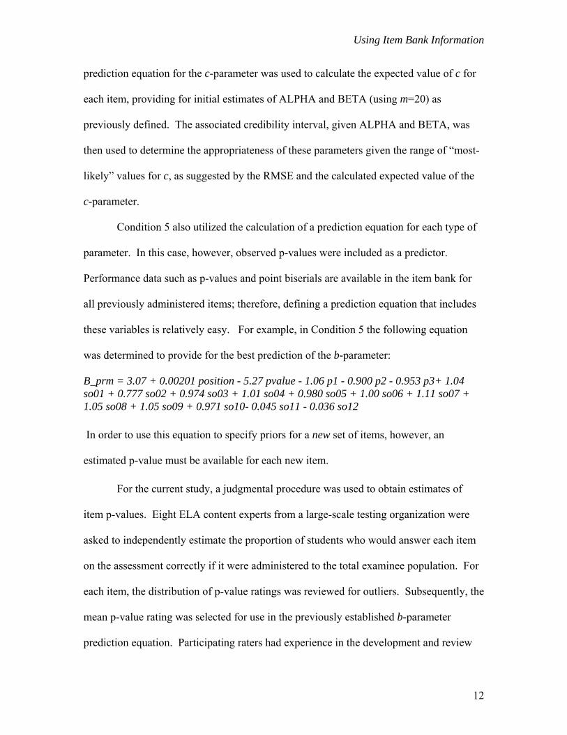
prediction equation for the c-parameter was used to calculate the expected value of c for
each item, providing for initial estimates of ALPHA and BETA (using m=20) as
previously defined. The associated credibility interval, given ALPHA and BETA, was
then used to determine the appropriateness of these parameters given the range of “most-
likely” values for c, as suggested by the RMSE and the calculated expected value of the
c-parameter.
Condition 5 also utilized the calculation of a prediction equation for each type of
parameter. In this case, however, observed p-values were included as a predictor.
Performance data such as p-values and point biserials are available in the item bank for
all previously administered items; therefore, defining a prediction equation that includes
these variables is relatively easy. For example, in Condition 5 the following equation
was determined to provide for the best prediction of the b-parameter:
B_prm = 3.07 + 0.00201 position - 5.27 pvalue - 1.06 p1 - 0.900 p2 - 0.953 p3+ 1.04 so01 + 0.777 so02 + 0.974 so03 + 1.01 so04 + 0.980 so05 + 1.00 so06 + 1.11 so07 + 1.05 so08 + 1.05 so09 + 0.971 so10- 0.045 so11 - 0.036 so12 In order to use this equation to specify priors for a new set of items, however, an
estimated p-value must be available for each new item.
For the current study, a judgmental procedure was used to obtain estimates of
item p-values. Eight ELA content experts from a large-scale testing organization were
asked to independently estimate the proportion of students who would answer each item
on the assessment correctly if it were administered to the total examinee population. For
each item, the distribution of p-value ratings was reviewed for outliers. Subsequently, the
mean p-value rating was selected for use in the previously established b-parameter
prediction equation. Participating raters had experience in the development and review
12
Using Item Bank Information
of ELA test items, as well as the interpretation of classical item statistics such as the p-
value and point biserial. Some raters had direct experience working with the specific
standards and objectives associated with the assessment of interest. To obtain the best
ratings possible, participating judges attended a brief training session intended to help
them gain a better understanding of the assessment program, examinee population of
interest, and estimation tasks before making their ratings.
Once prior distributions for item parameters were determined, BILOG-MG’s
marginal maximum a posteriori (MMAP) procedure was used for item parameter
estimation.
Determining Estimation Accuracy and Precision
To allow for the comparison of parameters across conditions, estimates were
scaled by standardizing on theta, as described in Kolen and Brennan (2004). To explore
the accuracy with which individual item parameters were estimated. First, within each
condition, correlations between estimated and baseline parameter values were calculated
to determine the extent to which they displayed the same relative order. Second, the
square root of the average mean squared difference (over items) between estimated and
baseline parameter values was obtained (RMSD).
The correlation coefficient and the RMSD jointly address how well baseline
parameters can be reproduced; however, neither speaks to the issue of estimation
precision. Such discussions require an analysis of standard errors. To facilitate an
interpretation of the standard error in terms of gains in precision within each sample (e.g.,
small/representative), or reduction in the standard error, the estimated percentage gain in
measurement precision relative to that obtained under the BILOG-MG default estimation
13
Using Item Bank Information
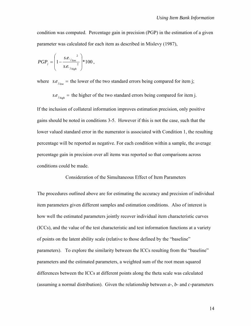
condition was computed. Percentage gain in precision (PGP) in the estimation of a given
parameter was calculated for each item as described in Mislevy (1987),
100*..
..1 2
2
⎟⎟
⎠
⎞
⎜⎜
⎝
⎛−=
highj
lowjj es
esPGP ,
where the lower of the two standard errors being compared for item j;
the higher of the two standard errors being compared for item j.
=lowjes.
=highjes.
If the inclusion of collateral information improves estimation precision, only positive
gains should be noted in conditions 3-5. However if this is not the case, such that the
lower valued standard error in the numerator is associated with Condition 1, the resulting
percentage will be reported as negative. For each condition within a sample, the average
percentage gain in precision over all items was reported so that comparisons across
conditions could be made.
Consideration of the Simultaneous Effect of Item Parameters
The procedures outlined above are for estimating the accuracy and precision of individual
item parameters given different samples and estimation conditions. Also of interest is
how well the estimated parameters jointly recover individual item characteristic curves
(ICCs), and the value of the test characteristic and test information functions at a variety
of points on the latent ability scale (relative to those defined by the “baseline”
parameters). To explore the similarity between the ICCs resulting from the “baseline”
parameters and the estimated parameters, a weighted sum of the root mean squared
differences between the ICCs at different points along the theta scale was calculated
(assuming a normal distribution). Given the relationship between a-, b- and c-parameters
14
Using Item Bank Information
(i.e., how the size of one parameter affects the others) two sets of parameter estimates for
the same item may appear extremely different (based on relative size) but result in
equivalent ICCs along the bulk of the theta distribution (with the largest differences
occurring at the extremes where the fewest students are located). For this reason, a
weighted sum of the RMSD between the ICCs, rather than an average, was taken over
quadrature points. This resulted in one value summarizing the difference between the
ICCs over items and quadrature points for each sample/condition.
To summarize the difference between “baseline” and estimated test characteristic
curves, a weighted sum of the absolute differences between the values of the test
characteristic function at q specified quadrature points was computed. This index
provides information regarding the number of raw score points, on average, by which
estimated and baseline true scores differ. True score values are often used to support
scoring and equating, therefore, this index provides information about the extent to which
measurement error might be affecting these activities.
At a given theta value, or quadrature point, the value of the test information
function is a measure of the degree of precision in estimating theta afforded by the
selected set of assessment items. The test information function is often used in test
construction to support development of equivalent assessments (in terms of estimation
precision) from year to year, and ensure appropriate levels of measurement precision
along the entire range (or a few specified points) of the ability. To understand the extent
to which differences between estimated and baseline parameters might influence
estimation precision, a weighted sum of the absolute difference between the two
respective test information functions was calculated for each condition.
15

Using Item Bank Information
Results
Summary of Examinee Population and Research Samples
Table 2 summarizes the performance of the “baseline” examinee population on the grade
7 ELA assessment reviewed for this study. This is the population from which all research
samples were subsequently selected.
-------------------------------- Insert Table 2.
--------------------------------
In terms of raw scores, Hispanic students earned (on average) ten fewer points than Non-
Hispanic students. In addition, their average estimated ability was approximately ¾ of a
logit below that of their Non-Hispanic peers. Standard deviations for total scores and
estimated abilities were slightly larger in the Hispanic sub-population; however, both
groups displayed a significant degree of variability. Consequently, range restriction, with
respect to student ability on the construct measured by this assessment, was not an issue
in either sub-population.
For each of the twelve sample types (e.g., ‘small/representative”), relationships
between sub-group means and standard deviations were comparable to those observed in
the population. Such similarities are to be expected given the within sub-population
random sampling procedure used to establish these samples. In addition, within a given
sample size (e.g., 100, 200, 500, 1000) unrepresentative samples were consistently the
most heterogeneous in terms of estimated ability and obtained raw score.
Summary of Preliminary Analyses
Several analyses were required to determine the prior distributions to be applied
in the estimation of item parameters under each of the proposed estimation conditions.
16

Using Item Bank Information
Only Conditions 1 and 2, in which BILOG-MG default prior distributions and baseline
calibration prior specifications were utilized, required no additional consideration before
use. This section provides a summary of the data reviewed and analyses performed to
define the prior item and ability distributions for the three remaining estimation
conditions.
The final set of common item parameter prior distributions applied in Condition 3
are provided in Table 3. For comparison purposes this table also provides the BILOG-
MG default and baseline calibration prior specifications. Together they represent the
three varieties of common prior specifications (over items) used in this study.
-------------------------------- Insert Table 3
-------------------------------- Condition 3 and its associated item bank prior distributions differ from the other common
prior conditions in three important ways. First, Condition 3 is the only common-prior
condition (i.e., one in which the same prior is applied across all items) in which a prior is
specified for the b-parameter. Second, relative to the default prior conditions, Condition
3 provides for a more informative a-parameter prior distribution (as suggested by the
smaller standard deviation) with a lower expected value. Finally, the expected value of
the c-parameter is much lower in Condition 3 than in the other common-prior conditions.
Priors Based on Collateral Item Variables (Conditions 4 & 5)
The percentage of total item parameter variance explained by each readily
available collateral variable and each category of collateral information is provided in the
top half of Table 4.
-------------------------------- Insert Table 4.
--------------------------------
17
Using Item Bank Information
Of the readily-available variables (i.e., 1-5), content specification (i.e., measured skill or
objective as defined by the test blueprint) produced the largest multiple correlation
(percent explained variance) with log of a-parameter and c-parameter estimates. Given
13 different objectives represented by 12 dummy variables, however, the proportion of
parameter estimate variance explained by this variable was only marginally significant
(e.g., 0.20<p<0.25). The variable “item position” provided for the most significant F-
statistic with respect to explained a-parameter variance (p<0.001); and the categorical
variable passage type (represented by 3 dummy variables) was the most significant with
respect to c-parameter variance (p<.02). Passage-type also produced the most significant
multiple correlation with estimated b-parameters (p=.002). The four different types of
passages utilized for this assessment were: literary, functional, informational, and
writing.
With respect to the final prediction equations used to estimate item-level prior
means in Condition 4, the set of collateral variables selected for inclusion explained
approximately 17%, 18%, and 15% of the variance in the item bank for estimated a-, b-,
and c-parameters. The average squared deviation between predicted and observed
parameter estimates (RMSE) applied as the common prior standard deviation for each
type of parameter was 0.26, 0.71 and 0.08 for log of a, b and c-parameters, respectively.
In addition, correlations between predicted and baseline values were 0.05, 0.26 and 0.35
for the log of a-parameters, b-parameters, and c-parameters, respectively. This is not
surprising. The small amount of a-parameter variance explained by the established
regression model provided for a relatively homogeneous set of predicted a-parameters.
This, in turn, resulted in small correlations between baseline and predicted values. On
18
Using Item Bank Information
the other hand, for both the b- and c-parameters there was a moderate correlation between
predicted and observed values. This is true in light of the small percentage of variance
accounted for by the regression model.
In Condition 5, p-values (i.e., 6 in Table 4) were considered in addition to readily-
available variables in determining the prediction equations and RMSEs to be used in
specifying item-level prior distributions. For b-parameter estimates, the contribution of
the p-values, given the previously defined set of relevant “readily available” variables
was extremely significant (p<.0001). While not nearly as influential, p-values also
contributed to the explanation of a- and c-parameter variance above and beyond that
previously accounted for by the readily-available variables. In Condition 5 the
percentage of variance jointly explained by readily available variables and p-values, as
represented by the applied prediction equations, was 23%, 85% and 16% for a-, b-, and c-
parameters, respectively. Associated RMSEs were 0.26, 0.31, and 0.09; and correlations
between predicted and baseline parameter values were 0.19, 0.24 and 0.31, respectively.
To make use of a prediction equation that includes p-values, estimates of these
variables must be available for the set of items to be calibrated. In the current study,
estimates of p-values were obtained using content expert ratings of item difficulty. One
major problem with this technique is that ratings of item difficulty (or p-values) are not as
reliable as observed p-values in predicting IRT parameter estimates, and therefore may
not accurately represent the relationship (between observed p-values and IRT parameters)
reflected in the regression model. This could produce inappropriate, biased estimates of
prior means and (subsequently) estimated parameters, because the small RMSE
19

Using Item Bank Information
associated with a model using observed p-values will constrain estimates to a narrower
range around their prior values.
To determine the appropriateness of the linear regression models defined for
Conditions 4 and 5, standardized residual plots and histograms based on the predicted and
observed parameter estimates in the item bank were reviewed. In general, results
supported the standard regression assumption that errors are normally distributed with
mean equal to zero. There were no extreme outliers; quantiles of residuals were
comparable to quantiles of the normal distribution; and the shape of the residual
histogram displayed the desired bell-shape. In consideration of these results, the
prediction equations were deemed appropriate for use in generating item-level prior
means and Beta parameters.
Table 5 lists the prior standard deviations applied in each of the estimation
conditions examined for this study.
-------------------------------- Insert Table 5.
--------------------------------
Smaller standard deviations imply more confidence in the prior mean as a predictor of the
parameter, and consequently, a smaller range of “reasonable” parameter estimates. Since
different Beta prior distributions were applied to each item in Conditions 4 and 5, the
average ALPHA and BETA parameters over items were used to calculate a “typical”
prior standard deviation for each of these conditions.
The b-parameter prior standard deviation applied in Condition 5 was clearly the
smallest. With a value of 0.31 it was less than half the size of those applied in Conditions
3 and 4. This is to be expected given the noted strong relationship between observed p-
20

Using Item Bank Information
values and b-parameter estimates in the item bank, which resulted in a small RMSE. On
the other hand, a-parameter prior standard deviations were similar across Conditions 3, 4,
and 5 averaging approximately half the size of the prior applied under Condition 1. C-
parameter prior standard deviations were extremely similar over conditions, differing on
average by less than 0.01.
Parameter Estimation Results
Very few consistent results (across samples and conditions) were identified
through the examination of correlations. In general, correlations increased as sample
sizes got larger; however across samples and parameter types there was no one condition
that provided for the highest correlations with baseline parameters. Estimated a-
parameters showed moderate to large correlations with baseline parameters, ranging from
0.43 - 0.91. Correlations between estimated and baseline b-parameters were relatively
high for all samples and all conditions (0.73- 0.98). While these correlations did increase
slightly with sample size, for the most part they were extremely similar across sample
sizes and conditions. Correlations between estimated and baseline c-parameters were
poor to moderate (-0.27 to 0.65). This is to be expected given the small range of
operational values associated with this parameter, its tiny standard deviation (e.g., 95% of
the c-parameters in the item bank fall between 0.03 and 0.31 and the standard deviation is
only 0.09), and the restricted range of applied prior mean values.
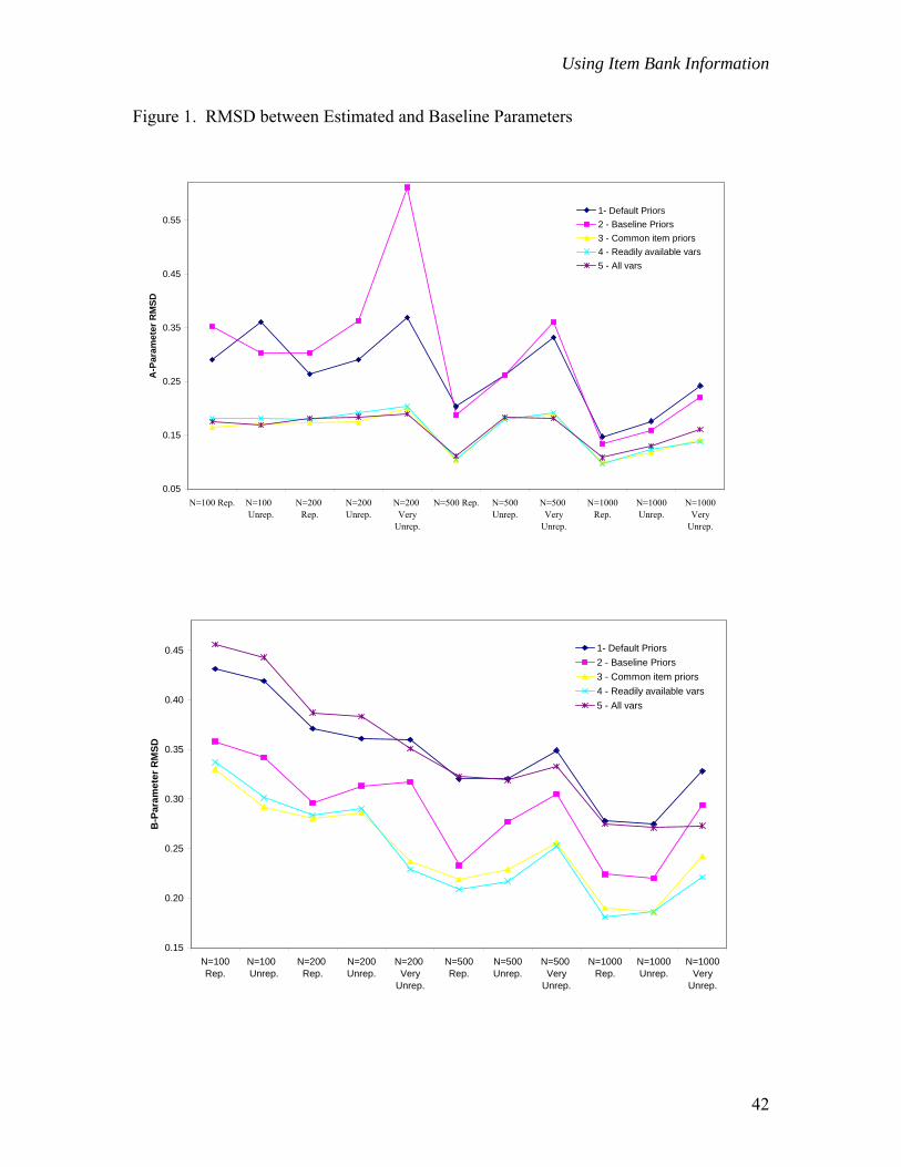
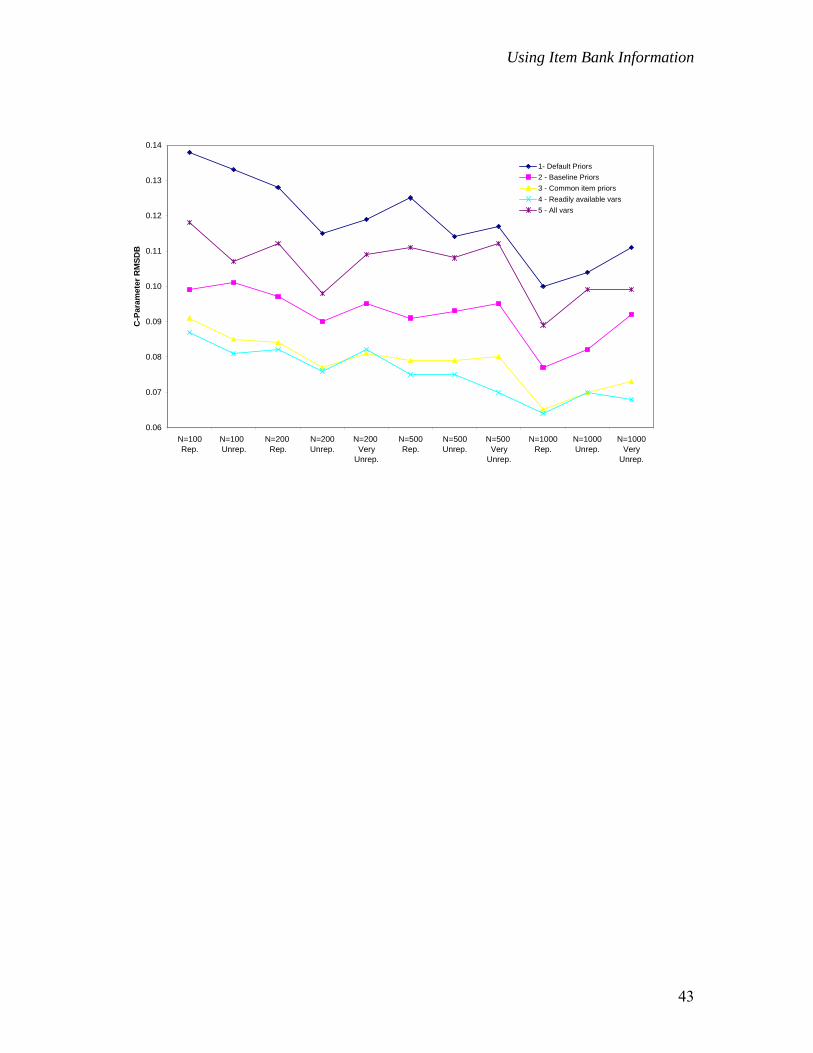
RMSD plots for each condition and parameter type are provided in Figure 1.1 To
lend some meaning to these values the average standard error of the estimate over items
1 Due to minor convergence problems, results are not presented for the n=100, very unrepresentative sample.
21
Using Item Bank Information
and conditions was computed for each sample. For example, the average standard error of
the b-parameter estimates in the N=200, representative sample was 0.253. The RMSD
associated with Condition 1 in this sample was 0.371. Estimated and baseline b-
parameters for this sample and condition therefore differed on average, by approximately
1.5 standard errors.
For all samples and parameter types, Conditions 3 and 4, which made use of
readily available collateral information about items, produced the smallest RMSD values.
On average, these values were 0.50 to 0.75 standard errors smaller than those associated
with Condition 1 (default priors). In fact, Condition 4 RMSD values for the two smallest
sample sizes were often comparable to, or less than, the RMSD values for the two larger
samples under both default and baseline prior conditions (i.e., Conditions 1 and 2). For
example, Condition 4 RMSDs for the n=100, representative group were 0.182, 0.337, and
0.087 for a-, b- and c-parameters respectively. These RMSD values are smaller than
those obtained in Condition 1 with a sample size of 500 for the a-parameter, 200 for the
b-parameter, and 1000 for the c-parameter.
Within a sample type (e.g., representative) both RMSD values and standard errors
tended to decrease as sample size increased. The effect of group representation on
accuracy, however, was typically inconsistent, and differed by parameter type.
Simultaneous Consideration of all Estimated Parameters
Figure 2 provides a plot of the average difference in the ICCs generated using the
estimated parameters and the baseline parameters from the total population calibration.
------------------------------ Insert Figure 2
-----------------------------
22
Using Item Bank Information
Overall, Conditions 3 and 4 provided for the smallest average deviations between
baseline and estimated ICCs. This was true across sample sizes and types. Within a
sample type (e.g., representative, unrepresentative, very unrepresentative) differences in
ICCs tended to decrease as sample sizes increased and within a sample size (e.g., 500),
differences in ICCs tended to increase as samples became more unrepresentative of the
population. In fact, medium sized samples (N=500) that represented the population often
provided for smaller ICC deviations than large unrepresentative samples. For example,
in Condition 4 the ICC deviation for the N=500, representative sample is 30% smaller
than the deviation associated with the N=1000, very unrepresentative sample and
equivalent to the deviation associated with the N=1000, unrepresentative sample.
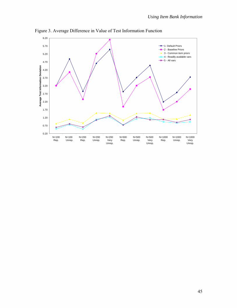
Figure 3 provides a plot of the weighted sum, over quadrature points, of the
absolute difference in the value of the test information function.
------------------------------ Insert Figure 3
-----------------------------
These deviations are intended to provide an index of how close the estimated test
information function (as calculated using the estimated parameters from each condition)
came to the “baseline” test information function. They do not offer any information
regarding directionality; that is, whether a particular condition provided for more or less
information (on average) than that obtained in the baseline calibration. This was done
intentionally. Information is calculated as a function of item parameters and theta, and
the value of the information function is typically greatest at that point on the underlying
scale where the most items are located. Consequently, a condition that results in a
homogeneous set of parameter estimates with difficulties concentrated around the middle
23
Using Item Bank Information
of the theta scale could produce larger values of information around this area of the scale
than those calculated with the baseline parameters. Since the estimates do not accurately
reflect the “true” or baseline parameters, however, this increase in information would not
imply the estimated parameters are better, or more precise, than the baseline parameters.
The difference between these two values is simply a way of looking at the extent to
which results based on estimated parameters deviate from results based on baseline
parameters.
In all conditions that made use of collateral item information (i.e., 3, 4, 5),
deviations were substantially smaller than those seen in Conditions 1 and 2. Condition 4
deviations in the smallest sample (n=100) were all less than the deviations obtained with
the largest sample in Conditions 1, 2, or even 3. In addition, Condition 1 deviations
which utilized default BILOG-MG priors were, on average, 4.5 times larger than those
seen in Condition 4. Also noteworthy is the fact that test information deviations tended
to increase as samples became more unrepresentative. This was true over sample sizes
and conditions, but was most pronounced in those conditions for which collateral
information was not used in the specification of priors (i.e., 1 and 2).
The weighted sum (over quadrature points) of the absolute difference in the value
of test characteristic function (estimated true score) based on baseline and estimated
parameters is plotted in Figure 4.
------------------------------ Insert Figure 4
-----------------------------
Trends in TCC deviations were extremely similar to those identified for test information:
over sample sizes and types, Condition 4 provided for the smallest TCC deviations, and
24
Using Item Bank Information
TCC deviations increased as sample size and sample representation decreased. For a
given sample, Conditions 3, 4, and 5 deviations often differed by only one-tenth of a raw
score or less. Condition 1 deviations, however, were typically one-half to three-fourths
of a raw score point greater than those obtained in Condition 4.
Percentage Gained in Precision – Reduction in Standard Error
For each condition, the percentage gained in precision (PGP) was calculated with
respect to the standard errors associated with the parameter estimates from Condition 1.
Condition 1 estimates represent those that would typically be obtained in practice if no
collateral information was used to support the specification of prior distributions. It was
expected that those conditions in which the most informative priors were specified would
provide for the largest gains in precision, (or smallest standard errors), since estimates
were constrained to a smaller range of possible values. Since the more informative priors
were typically associated with the collateral item information conditions (3-5), it was
expected that for these conditions gains would be mainly positive. Of greater interest,
therefore, was: 1) How did conditions with similar prior standard deviations compare in
terms of gains in precision, and 2) What, if any, patterns were observable within a given
condition?
The prior standard deviations applied in each estimation condition are provided in
Table 5. A-parameter prior standard deviations in Conditions 3-5 were all relatively
similar (i.e., 0.30, 0.26, and 0.26, respectively) compared to the larger prior standard
deviation applied in Condition 1 (i.e., 0.60). For the b-parameter, the specified prior
standard deviation was the same in Conditions 3 and 4 (i.e., approximately 0.72),
relatively small in Condition 5 (i.e., 0.31, for n=64), and not specified in Condition 1.
25
Using Item Bank Information
On average, c-parameter prior standard deviations were smaller in Conditions 3-5 than in
Condition 1.
Figure 5 presents the average percent gained in precision (over items) relative to
Condition 1 for each parameter-type by sample size and condition.
------------------------------ Insert Figure 5
----------------------------- In general, small samples benefited the most from the utilization of collateral item
information (in terms of PGP). Within a given sample type (e.g., representative,
unrepresentative), PGPs tended to decrease as sample sizes increased. This was true for
all three types of parameters, but most pronounced for a- and c-parameters. In addition,
those conditions in which the smallest prior standard deviations were applied showed the
largest gains in precision relative to Condition 1. This was Conditions 4 and 5 for a-
parameters, Condition 5 for b-parameters, and Condition 4 for c-parameters.. To some
extent these results reflect the degree to which parameters were constrained in estimation.
For example, Condition 5 led to the least accurate estimates of b-parameters in terms of
correlations and RMSDs, but provided for the largest gains in precision.
Finally, although very similar prior standard deviations were applied in
Conditions 3 and 4 for the a- and b-parameters, gains in precision were consistently
higher in Condition 4. That is, in terms of PGP the use of collateral information to
specify item-level prior means improved estimation precision beyond that obtained
through the use of a common prior.
26

Using Item Bank Information
Summary
The overall goal of the current study was to explore how and if collateral variables and
information of the type typically found in an item bank, associated with a test blueprint,
or collected as part of a test administration, could be used to improve item parameter
estimation through the specification of more appropriate item parameter prior
distributions. In addressing this overall goal, several smaller research questions were
identified. These are addressed in turn in the remainder of this section:
1. Is parameter estimation in general influenced by sample size and sample representation? Results suggested that both sample size and sample representation influence
parameter estimation. Within a sample type (representative, unrepresentative, very
unrepresentative), correlations between estimated and baseline parameters tended to
increase and deviations (RMSD, ICC, Test Info, TCC) tended to decrease as sample sizes
increased.
This study provided little definitive information regarding the manner in which
sample representation influences the estimation of different types of item parameters.
There were two reasons for this. First, since only one sample was developed to represent
each sample size/representation condition, the effect of sampling error on estimation is
unknown. That is, it is unclear whether the results from a given sample are representative
of the results that would be observed with other samples of the same type. Second, due
to the similarity of Hispanic and Non-Hispanic students (with respect to observed ability
distributions), misrepresentative samples did not display those features shown to have a
negative effect on estimation, such as range restriction or skew (with respect to estimated
ability) (Ree, 1979). In fact, under some conditions, the characteristics of the
27
Using Item Bank Information
unrepresentative samples often served to improve estimation. Consequently, trends,
when identified, were often isolated to a particular type of parameter, index of accuracy,
and sample size; making them extremely difficult to interpret.
Although the effect of sample misrepresentation was often difficult to interpret at
the parameter level, at the test level some trends did emerge. In general, deviations
between test characteristics based on estimated and baseline parameters (e.g.,
information/estimated true scores) increased as sample representation decreased. This
was true for all sample sizes, suggesting that the potential influence of sample
misrepresentation on estimation cannot be ignored simply because one has a large
sample.
One possible explanation for this finding is a decrease in model fit for samples
that do not represent the population. For example, if the model fit less well for Hispanic
compared to Non-Hispanic students, samples in which Hispanic students were over-
represented would show greater model misfit. This would, in turn, have a negative
impact on the accuracy of item parameter estimates. Similarly, if differential item
functioning was a major problem, overrepresentation of the affected subpopulation would
have a negative impact on the accuracy of estimation. While model fit by ethnic group
was not explored in the current study, all items were reviewed for differential item
functioning.
2. Does the use of readily available collateral item information to support the specification of priors consistently improve estimation accuracy and precision? How does this differ depending on the characteristics of the sample? In this study, the conditions that utilized collateral item information in the
specification of priors (i.e., Conditions 3, 4, and 5) produced the most accurate and
28
Using Item Bank Information
precise estimates of parameters over sample sizes and types. Although correlations
provided no consistent information, average squared deviations between estimated and
baseline parameters from these conditions were consistently smaller (over all samples
and both test lengths) than those obtained under other conditions. Similarly, deviations
between baseline and estimated item characteristic curves, test characteristic curves, and
test information functions were noticeably smaller for the collateral information
conditions.
For the current study, item-level priors and standard deviations based on readily
available collateral information (Condition 4) were quite similar to (albeit a little smaller
than) the common item bank priors. This is likely due to the small percentage of
parameter variance explained by the collateral variables and regression to the mean.
Consequently, these conditions provided for very similar results with respect to
correlations, RMSDs and ICC deviations. However, in terms of test information and
TCC deviations Condition 4 did provide for slightly more accurate results.
The extent to which collateral information improved estimation accuracy (relative
to default conditions) did not appear to differ by sample size. On average, gains were
about the same for all sample sizes. This is readily apparent through a review of RMSDs.
While deviations between estimated and baseline parameters were significantly smaller in
Condition 4 compared to Condition 1, the extent to which these deviations differed (in
standard error units) did not consistently increase as sample size decreased. B-parameter
deviations from Condition 1 might be three-tenths of a standard error larger than
Condition 4 deviations when N=200, but six-tenths of a standard error larger when
N=1000. Similar results were noted for ICC and TCC deviations. The ratio of
29
Using Item Bank Information
Condition 1 to Condition 4 deviations did not consistently increase as sample size
decreased. Only with respect to test information did this ratio show a slight tendency to
increase as sample size decreased.
Similarly, the extent to which collateral information improved estimation did not
appear to be related to sample representation All sample types benefited from the use of
priors based on collateral information such that within a sample size, ratios of Condition
1 to Condition 4 deviations did not consistently increase as samples became more
unrepresentative. The only exception to this was test information, for which these ratios
did show a tendency to increase as sample representation decreased.
Although gains in estimation accuracy afforded by the use of collateral variables
(relative to Condition 1), were not affected by group representation; the stability of the
results provided over different types of samples was. That is, use of a prior informed by
collateral information significantly lessened the (typically) negative effect of sample
representation on estimation. This was apparent mainly at the test level, through a review
of TCC and test information deviations. Within a given sample size, the difference
between test information deviations for unrepresentative and representative groups was 2
to 10 times greater in Condition 1 than Condition 4. Similarly, differences between very
unrepresentative and unrepresentative groups were 6 to 13 times larger in Condition 1
compared to Condition 4. Similar findings were obtained with respect to TCC
deviations. The use of prior distributions informed by collateral variables resulted in
more stable results across sample types.
3. Does the use of content-expert ratings of item difficulty improve the quality of estimated parameters when used in conjunction with readily-available variables to define item prior distributions?
30
Using Item Bank Information
In the current study, the use of content-expert ratings provided little value beyond
that afforded by readily available collateral variables. This was due to the difficulty of
the rating task and the accuracy of the resulting ratings in comparison to observed p-
values. Since p-value ratings were not as reliable as observed p-values for predicting the
values of parameter estimates, regression models developed using observed p-values did
not improve estimates of prior means as intended (especially for b-parameters). In
addition, given the strong relationship between observed p-values and b-parameters,
applied b-parameter prior standard deviations were extremely small resulting in less
accurate estimates of parameters than were obtained in the other collateral information
conditions. Since the b-parameter is relatively resilient to different prior specifications
(Swaminathan & Gifford, 1982; Gao & Chen, 2005), however, the overall influence of
these priors on test and item characteristics was minimal and these estimates still
recovered item and test characteristics better than did estimates generated under the non-
collateral item information conditions (i.e., Conditions 1 and 2).
Together these results suggest that the use of content expert ratings may improve
the quality of estimated parameters, however the degree of improvement depends on their
accuracy and the manner in which they are used. Since accurate and reliable ratings of
item difficulty are difficult to obtain, and may be of only limited usefulness, gathering
this information for the sole purpose of informing prior distributions is not recommended.
If, however, difficulty ratings of some sort are available (from a standard setting or some
other kind of committee meeting) and one has a high degree of confidence in their
accuracy, they may be considered for use as described above (or in some other fashion).
31
Using Item Bank Information
4. Do more informative priors always lead to item parameter estimates having smaller standard errors? Are smaller standard errors always associated with more accurate estimates of baseline parameters?
In general, for those conditions in which a prior distribution was specified for
item parameters, the more informative the prior (i.e., the smaller the standard deviation),
the greater the gain in estimation precision. This was true even when the estimated
parameters were less accurate than those obtained in other conditions.
Discussion
Consistent with previous research (e.g., Swaminathan, et. al., 2003; Mislevy,
1988) the results of the current study show that using collateral item information to
inform item prior specifications provides for improved estimates of item parameters.
Both common priors based on item bank means and standard deviations, and item-level
priors based on collateral item-variables, provided for more accurate and precise
estimates of parameters than were obtained in other conditions. The fact that priors based
on collateral information provided better estimates than the use of BILOG-MG default
priors is, in and of itself, an important finding for two reasons. First, BILOG-MG item
prior specifications are not uninformed or arbitrary; they are based on the program
authors’ experience and educated opinion regarding which prior distributions are
appropriate in most situations in the absence of other useful information. And second,
these are the prior specifications most often applied in practice.
Of particular interest is the fact that the consideration of readily available
collateral variables, of the type that would always be available for a test item (ie., key,
position, reportable content category), provided better estimates of parameters than those
obtained in other conditions. This is true in light of the fact that these variables explained
32
Using Item Bank Information
a relatively small percentage of parameter variance (less than 17%), suggesting that even
a little good information is better than no information when it comes to the specification
of priors.
The use of item difficulty ratings in addition to readily available variables has the
potential for further improving estimation. Swaminathan (2003) showed that transformed
estimates of item difficulty ratings improved estimates of a-, b-, and c- parameters when
applied as prior means for b-parameters. The current study used regression procedures to
incorporate p-value ratings into the specification of prior means for b-parameters as well
as a- and c- parameters. Although p-value ratings were only slightly correlated with
observed p-values, priors generated in consideration of these ratings (Condition 5)
typically provided better estimates of item and test characteristics than did default priors.
The fact that improved estimates were obtained in light of these issues, suggests that the
defined regression procedure for establishing prior means in consideration of p-value
ratings may be appropriate under some conditions (e.g., when one has a great degree of
confidence in the ratings and a procedure for establishing the accuracy of the raters as a
group). Even then, however, a prior standard deviation based on something other than the
RMSE may be required.
The benefits of using collateral information in terms of gains in estimation
precision were readily apparent in the current study. The use of collateral information
reduced the standard errors of parameter estimates from those obtained under default
conditions. This was true in light of the relatively small percentage of parameter
variance explained by these variables. Percent gains in estimation precision varied by
parameter type, but consistently increased as sample size decreased. These gains were
33

Using Item Bank Information
often quite large, ranging from 23% for c-parameters to 26% for b-parameters to 60% for
a-parameters (N=100).
Overall, results provide support for the use of any high quality collateral
information that may inform the value of item operating characteristics. The call for
“high quality” information is not to be taken lightly. The use of item bank data, for
example, will only provide better prior specifications if the data in the bank are accurate
and representative of the parameters to be estimated.
Limitations
There are several limitations associated with the current study that constrain the
generalizability of results and suggest the need for further research. First, real, rather
than simulated, data were used to estimate item parameters; therefore true parameter
values were not known. Instead, estimates from the baseline calibration were treated as
“true”, or at least as the best estimates possible. In reality these estimates could contain
error related to lack of model data fit, item dependence (since items are passage-based),
differential item functioning (DIF), or other factors. In addition, only a single sample
was selected to represent each of the twelve sample size/ethnic representation
combinations of interest to this study. This limits the generalizability of results because
the effect of sampling error is unknown. Further, this design does not allow for the
examination of deviations between estimated and baseline parameters in terms of
separate bias and sampling error components. For this reason, while Condition 4 may
provide for smaller RMSDs between estimated and baseline parameters (for example), it
is not known that this condition produces “better” results. These estimates may still be
more biased than those obtained under other conditions.
34

Using Item Bank Information
The conditions of this study should be replicated using simulated data and
multiple samples. In this way, true item parameters and student abilities would be
known, model fit would not be an issue, and deviations between true and estimated
values could be interpreted in terms of bias and sampling error components. In addition,
by simulating data sets, a variety of different sample characteristics could be modeled
with respect to the underlying theta distribution. This would provide cleaner, potentially
more generalizable results regarding the effects of sample characteristics on estimation
accuracy.
A second limitation relates to the PGP index. Because it is tied directly to the
size of the prior standard deviation, percent gained in precision (as calculated) is not a
particularly good indicator of the quality of the applied estimation procedure and
resulting parameters. In fact, in isolation, such an index may provide for misleading
results regarding which prior specification and estimation procedure is most effective.
Consequently, an index that reflects gains in precision afforded by the use of an
informative prior, but is not itself defined by that prior, needs to be identified.
Consideration of the entire posterior distribution associated with a parameter, for
example, may provide for a useful index.
A final issue relates to the fact that BILOG-MG (and other programs like it) often
define item parameters in terms of point-estimates from posterior distributions. This,
however, is not the preferred Bayesian procedure for estimating parameters because it
does not use the entire posterior distribution. Rather, an empirical Bayes approach in
which simulated observations from a Markov Chain are used to make inferences about
IRT item parameters might be endorsed (Patz & Junker, 1999). Although some research
35

Using Item Bank Information
has shown Markov Chain Monte Carlo (MCMC) procedures to be superior to those
implemented in BILOG in terms of IRT model fit (Jones & Nediak, 2000), for the most
part, the use of such procedures is currently limited to complex IRT models (e.g., multi-
dimensional). Additional research is required to explore the potential benefits of using
MCMC procedures for the estimation of IRT parameters in general, and in light of
available collateral item and examinee information.
Conclusion
This study provided evidence for the use of collateral item information in the
specification of item prior distributions. In addition, it outlined a relatively
straightforward regression procedure for utilizing this information to define prior
distribution parameters. While the procedures discussed are based the use of BILOG-
MG for calibration, they can easily be adapted to support the requirements of other
related IRT calibration software.
The benefits of using high quality, readily available item information to improve
the specification of item prior distributions are clear: improved estimation accuracy and
precision for samples of all types and sizes. Up to this point, however, the specific
context within which procedures using collateral information might be applied has not
been discussed. There are a range of item parameter estimation situations for which these
procedures may be appropriate. These situations vary in terms of the stakes associated
with inappropriate estimation, and the degree to which the procedures generalize over
assessment programs and materials. One situation for which these procedures seem
extremely appropriate is to support the estimation of field-test item parameters intended
36
Using Item Bank Information
for use in test development activities. More debatable situations for the use of collateral
information include supporting:
the estimation of item parameters to be used in scaling and/or equating activities;
the estimation of operational item parameters that will be used for scoring
examinees; and
the use of collateral information from one assessment program to support the
specification of prior item parameter distributions for another assessment
program (for use in test development, scaling, equating , or scoring activities
Further research is required to understand the range of situations to which these
procedures may apply.
37

Using Item Bank Information
References
Birnbaum, A. (1968). Some latent trait models and their use in inferring an examinee’s ability. In F. M. Lord & M.R. Novick (Eds.), Statistical theories of mental test scores (pp.397-472). Reading, MA: Addison-Wesley.
Gao, F., & Chen, L. (2005) Bayesian or Non-Bayesian: A Comparison Study of Item Parameter Estimation in the Three-Parameter Logistic Model. Applied Measurement in Education, 18(4), 351-380.
Gifford, J.A., & Swaminathan, H. (1990). Bias and the effect of priors in Bayesian estimation of parameters of item response models. Applied Psychological Measurement, 14, 33-43.
Hambleton, R.K. (1989) Principles and Selected Applications of Item Response Theory. In R. L. Linn (Ed.), Educational measurement (3rd ed.)(pp. 147-199). New York: American Council on Education and Macmillan.
Jones, D.H., & Nediak, M.S. (2000). Item parameter calibration of LSAT items using MCMC approximation of Bayes posterior distributions. Research Report, Rutgers the State University of New Jersey: Faculty of Management and RUTCOR [on line]. Available: http://rutcor.rutgers.edu/pub/rrr/reports2000/07.pdf
Kolen, M. J., & Brennan, R. L. (2004). Test equating, scaling, and linking: Methods and practices. (2nd ed.) New York: Springer-Verlag.
Lord, F.M. (1986). Maximum likelihood and Bayesian parameter estimation in item response theory. Journal of Educational Measurement, 23 (2), 157-162.
Mislevy, R.J. (1986). Bayes modal estimation in item response models. Psychometrika, 51, 177-195.
Mislevy, R.J., (1988). Exploiting auxiliary information about items in the estimation of Rasch item difficulty parameters. Applied Psychological Measurement, 12 (3), 281-296.
Mislevy, R.J., Sheehan, K.M., & Wingersky, M. (1993). How to equate tests with little or no data. Journal of Educational Measurement, 30 (1), 55-78.
Patz, R. J., & Junker, B. W. (1999a). A straightforward approach to Markov chain Monte Carlo methods for item response models. Journal of educational and behavioral statistics. 24, 146-178.
Ree, M.J. (1979) Estimating Item Characteristic Curves, Applied Psychological Measurement, 3 (3), 371-386.
38
Using Item Bank Information
Swaminathan, H., & Gifford, J.A. (1982). Bayesian estimation in the Rasch model. Journal of Educational Statistics, 7, 175-191.
Swaminathan, H., & Gifford, J.A. (1985). Bayesian estimation in the two-parameter logistic model. Psychometrika, 50, 349-364.
Swaminathan, H., & Gifford, J.A. (1986). Bayesian estimation in the three-parameter logistic model. Psychometrika, 51, 589-601.
Swaminathan, H., Hambleton, R.K., Sireci, S.G., Xing, D. & Rizavi, S.M. (2003). Small sample estimation in dichotomous item response models: Effect of priors based on judgemental information on the accuracy of item parameter estimates. Applied Psychological Measurement, 27 (1), 27-51.
39
Using Item Bank Information
Table 1. Parameter Estimation Conditions
Source of Item Parameter Prior Information
Common Prior Over
Items?
Con
ditio
n
BILOG-MG
Defaults
Population Baseline
Calibration
Item Bank Parameter
Means and SDs
Readily Available Collateral Variables
Readily Available & Difficulty Ratings Y N
1 x x 2 x x 3 x x 4 x x 5 x x
Table 2. Summary of Population Performance on Total Test
Bayes Estimate of Ability (EAP)
Total Score (n=64)
N Mean Std. Dev.
Median Mean Std. Dev. Median
Total Population 33347 0.000 0.976 0.248 45.598 12.201 49 Not Hispanic 29484 0.089 0.942 0.369 46.745 11.624 50
Hispanic 3863 -0.680 0.964 -0.478 36.847 12.932 37
Table 3. Common-Prior Means and Standard Deviations by Source
Source of Prior a b c
Default BILOG-MG Priors
(Condition 1)
N(1.13, 0.60) none Beta(6,16) mean=0.25 SD=0.094
Population Baseline Calibration Priors
(Condition 2)
none none Beta(5,17) Mean=0.20 SD=0.087
Item Bank Parameter Estimate Means and SDs
(Condition 3) N(0.84, 0.30) N(-0.58, 0.75)
Beta (3.4, 13.6) Mean=0.15
SD=.087
40

Using Item Bank Information
Table 4. Percentage of Item Parameter Variance Explained by Collateral Variables
Variable(s) b-parameter Log of a-parameter c-parameter
1. Position 0.35 5.82 0.02 2. Key 1.24 1.15 3.64 3. Passage type* 8.13 1.81 5.40 4. Passage length 0.22 0.23 0.82 5. Skill/Objective (Content-related) 6.38 8.55 8.22 Adminstration-related (1&2) 1.56 7.28 3.65 Passage related (3&4) 8.39 2.06 5.43 All readily-available (1-5) 20.79 17.48 15.62 6. P-value 82.15 8.89 2.62
*The four passage types utilized for this assessment were: Functional, Literary, Informational, and Writing. Table 5: Item Parameter Prior Standard Deviations for a-, b-, and c-Parameters
Source of Priors
Condition applied
a b c
BILOG-MG defaults 1 0.60 NA 0.094 Baseline calibration 2 NA NA 0.087 Item Bank 3 0.30 0.75 0.087 Readily available variables 4 0.26 0.71 0.080 Readily available variables and p-values 5 0.26 0.31 0.092
41
Using Item Bank Information
Figure 1. RMSD between Estimated and Baseline Parameters
0.05
0.15
0.25
0.35
0.45
0.55
N=100 Rep. N=100 Unrep.
N=200 Rep.
N=200Unrep.
N=200 Very
Unrep.
N=500 Rep. N=500Unrep.
N=500 Very
Unrep.
N=1000Rep.
N=1000Unrep.
N=1000Very
Unrep.
A-P
aram
eter
RM
SD
1- Default Priors2 - Baseline Priors3 - Common item priors4 - Readily available vars5 - All vars
0.15
0.20
0.25
0.30
0.35
0.40
0.45
N=100Rep.
N=100 Unrep.
N=200 Rep.
N=200Unrep.
N=200 Very
Unrep.
N=500Rep.
N=500Unrep.
N=500 Very
Unrep.
N=1000Rep.
N=1000Unrep.
N=1000Very
Unrep.
B-P
aram
eter
RM
SD
1- Default Priors2 - Baseline Priors3 - Common item priors4 - Readily available vars5 - All vars
42
Using Item Bank Information
0.06
0.07
0.08
0.09
0.10
0.11
0.12
0.13
0.14
N=100Rep.
N=100 Unrep.
N=200 Rep.
N=200Unrep.
N=200 Very
Unrep.
N=500Rep.
N=500Unrep.
N=500 Very
Unrep.
N=1000Rep.
N=1000Unrep.
N=1000Very
Unrep.
C-P
aram
eter
RM
SDB
1- Default Priors2 - Baseline Priors3 - Common item priors4 - Readily available vars5 - All vars
43

Using Item Bank Information
Figure 2. Average Difference between Item Characteristic Curves (ICCs)
0.02
0.02
0.03
0.03
0.04
0.04
0.05
0.05
0.06
N=100Rep.
N=100 Unrep.
N=200 Rep.
N=200Unrep.
N=200 Very
Unrep.
N=500Rep.
N=500Unrep.
N=500 Very
Unrep.
N=1000Rep.
N=1000Unrep.
N=1000Very
Unrep.
Ave
rage
ICC
Dev
iatio
n
1- Default Priors2 - Baseline Priors3 - Common item priors4 - Readily available vars5 - All vars
44
Using Item Bank Information
Figure 3. Average Difference in Value of Test Information Function
0.20
0.70
1.20
1.70
2.20
2.70
3.20
3.70
4.20
4.70
5.20
5.70
6.20
N=100Rep.
N=100 Unrep.
N=200 Rep.
N=200Unrep.
N=200 Very
Unrep.
N=500Rep.
N=500Unrep.
N=500 Very
Unrep.
N=1000Rep.
N=1000Unrep.
N=1000Very
Unrep.
Ave
rage
Tes
t Inf
orm
atio
n D
evia
tion
1- Default Priors2 - Baseline Priors3 - Common item priors4 - Readily available vars5 - All vars
45

Using Item Bank Information
Figure 4. Average Difference between Test Characteristic Curves
0.10
0.20
0.30
0.40
0.50
0.60
0.70
0.80
0.90
1.00
1.10
1.20
1.30
N=100Rep.
N=100 Unrep.
N=200 Rep.
N=200Unrep.
N=200 Very
Unrep.
N=500Rep.
N=500Unrep.
N=500 Very
Unrep.
N=1000Rep.
N=1000Unrep.
N=1000Very
Unrep.
Ave
rage
TC
C D
evia
tion
1- Default Priors2 - Baseline Priors3 - Common item priors4 - Readily available vars5 - All vars
46
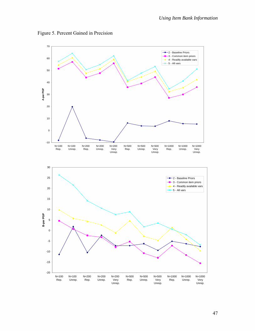
Using Item Bank Information
Figure 5. Percent Gained in Precision
-10
0
10
20
30
40
50
60
70
N=100Rep.
N=100 Unrep.
N=200 Rep.
N=200Unrep.
N=200 Very
Unrep.
N=500Rep.
N=500Unrep.
N=500 Very
Unrep.
N=1000Rep.
N=1000Unrep.
N=1000Very
Unrep.
A-p
ar P
GP
2 - Baseline Priors3 - Common item priors4 - Readily available vars5 - All vars
-20
-15
-10
-5
0
5
10
15
20
25
30
N=100Rep.
N=100 Unrep.
N=200 Rep.
N=200Unrep.
N=200 Very
Unrep.
N=500Rep.
N=500Unrep.
N=500 Very
Unrep.
N=1000Rep.
N=1000Unrep.
N=1000Very
Unrep.
B-p
ar P
GP
2 - Baseline Priors3 - Common item priors4 - Readily available vars5 - All vars
47

Using Item Bank Information
-25
-20
-15
-10
-5
0
5
10
15
20
25
N=100Rep.
N=100 Unrep.
N=200 Rep.
N=200Unrep.
N=200 Very
Unrep.
N=500Rep.
N=500Unrep.
N=500 Very
Unrep.
N=1000Rep.
N=1000Unrep.
N=1000Very
Unrep.
C-p
ar P
GP
2 - Baseline Priors3 - Common item priors4 - Readily available vars5 - All vars
48