exploringthespatio-temporalneuralbasisoffacelearn- ing - cmu …kass/papers/yangjov17.pdf ·...

Journal of Vision (20??) ?, 1–? http://journalofvision.org/?/?/? 1

Exploring the spatio-temporal neural basis of face learn-ing

Ying YangCenter for the Neural Basis of Cognition and Machine Learning Department

�Carnegie Mellon University, Pittsburgh, PA, USA

Yang XuDepartment of Linguistics, Cognitive Science Program

�University of California, Berkeley, Berkeley, CA, USA

Carol A. JewDepartment of Brain and Cognitive Sciences,

�University of Rochester, Rochester, NY, USA

John A. PylesCenter for the Neural Basis of Cognition and Department of Psychology


Robert E. KassDepartment of Statistics, Machine Learning Department and Center for the Neural Basis of Cognition


Michael J. TarrCenter for the Neural Basis of Cognition and Department of Psychology


Humans are experts at face individuation. Although previous work has identified a network of face-sensitive regions and

some of the temporal signatures of face processing, as yet, we do not have a clear understanding of how such face-sensitive

regions support learning at different time points. To study the joint spatio-temporal neural basis of face learning, we trained

subjects to categorize two groups of novel faces and recorded their neural responses using magnetoencephalography

(MEG) throughout learning. A regression analysis of neural responses in face-sensitive regions against behavioral learning

curves revealed significant correlations with learning in the majority of the face-sensitive regions in the face network, mostly

between 150-250 ms, but also post 300 ms. However, the effect was smaller in non-ventral regions (within the superior

temporal areas and prefrontal cortex) than that in the ventral regions (within the inferior occipital gyri (IOG), mid-fusiform

gyri (mFUS) and anterior temporal lobes). A multivariate discriminant analysis also revealed that IOG and mFUS, which

showed strong correlation effects with learning, exhibited significant discriminability between the two face categories at

different time points both between 150-250 ms and post 300 ms. In contrast, the non-ventral face-sensitive regions where

correlation effects with learning were smaller, did exhibit some significant discriminability, but mainly post 300 ms. In sum,

our findings indicate that early and recurring temporal components arising from ventral face-sensitive regions are critically

involved in learning new faces.

Keywords: learning, face individuation, spatio-temporal neural basis, MEG

doi: Received: March 23, 2017 ISSN 1534–7362 c© 20?? ARVO

Journal of Vision (20??) ?, 1–? Yang, Xu, Jew, Pyles, Kass, & Tarr 2

Introduction

Humans have extraordinary ability to recognize object categories and specific items within such categories. No where is this

more apparent than in the domain of face identification, where humans, almost universally, are capable of learning and remembering

thousands of individual human faces. Irrespective of whether face processing mechanisms are biologically hard-wired or not, and

whether they are in part or fully supported by domain-general learning mechanisms, acquiring such visual skills depends crucially on

learning over our lifespans (Bruce & Burton, 2002). Here we explore the neural basis of face learning by investigating which brain

regions, at what temporal stages in face processing, exhibit changes in neural activity as observers learn new, never-before-seen faces.

Previous research in functional magnetic resonance imaging (fMRI) has identified a spatial network of brain regions, known as the

“face network”, which underlies processing of faces at the individual level (Gauthier et al., 2000; Haxby, Hoffman, & Gobbini, 2000;

Nestor, Plaut, & Behrmann, 2011). In parallel, research using magnetoencephalography (MEG) or electroencephalography (EEG) has

identified a series of event-related temporal waveforms related to face processing (Liu, Higuchi, Marantz, & Kanwisher, 2000; Tanaka,

Curran, Porterfield, & Collins, 2006). However, we have a less than clear picture of the spatio-temporal structure of the neural activity

subserving both face processing and face learning. The research presented here studies the temporal stages and spatial locations where

neural activity correlates with learning new faces as part of a novel face categorization task. Particularly, we focus on comparing

the correlation with learning in the face-sensitive brain regions along the ventral visual pathway and in the higher-order face-sensitive

regions within the superior temporal areas and the prefrontal cortex at different temporal stages.

The face-sensitive regions comprise a “face network,” typically identified using fMRI. Critically, these brain regions at different

spatial locations are hypothesized to have different functional roles in face processing (Ishai, 2008; Pyles, Verstynen, Schneider, & Tarr,

2013). Figure 1 provides a visual illustration of the network. The ventral regions, including the “occipital face area” in the inferior

occipital gyrus (IOG) (Pitcher, Walsh, & Duchaine, 2011), the “fusiform face area” in the middle fusiform gyrus (mFUS) (Kanwisher,

McDermott, & Chun, 1997), and an area in the anterior inferior temporal lobe (aIT) (Kriegeskorte, Formisano, Sorger, & Goebel, 2007;

Nestor, Vettel, & Tarr, 2008; Rajimehr, Young, & Tootell, 2009), are located along the posterior to anterior direction within the ventral

visual stream (Mishkin, Ungerleider, & Macko, 1983). Notably, the ventral stream is hypothesized to be hierarchically organized,

featuring early to late, lower-level to higher-level visual processing along this same direction (DiCarlo & Cox, 2007). Under this

framework, IOG, mFUS and aIT are also likely to follow the ventral stream hierarchy in processing visual features of faces, supporting

face detection, categorization, and individuation. Other regions that are putatively part of the face network include posterior superior

temporal sulcus (STS), hypothesized to process the social aspects of faces (e.g., expression and gaze), and prefrontal regions in the

inferior frontal gyrus (IFG) and orbitofrontal cortex (OFC), hypothesized to process the semantic or valence-related aspects of faces

(Ishai, 2008). These presumed functions are supported by a rich fMRI literature on face processing qua face processing; however, only

a handful of fMRI studies have examined the role of the face network in face learning. For those studies, regions including IOG, mFUS

and prefrontal cortex, as well as hippocampus and basal ganglia have all been implicated as being involved in learning to categorize new

faces (DeGutis & D’Esposito, 2007, 2009), but detailed changes in dynamic cortical activity during learning have not been described —

primarily due to the inherently poor temporal resolution of fMRI.

In this same vein, a second line of work using EEG, a neuroimaging method characterized by high temporal resolution, has

identified several temporal waveforms that are face-sensitive: the P100 component at 100 ms after the stimulus onset appears to be

associated with face detection 1 (Cauchoix, Barragan-Jason, Serre, & Barbeau, 2014), the N170 peak at 170 ms is associated with

face detection and individuation (Cauchoix et al., 2014; Campanella et al., 2000), and the N250 component at 250 ms (or later) is

associated with facial familiarity (Tanaka et al., 2006). Several studies have also demonstrated that the face-sensitive waveforms at

170 ms, 200 ms, and ≥250 ms change in amplitude or latency during learning new object categories (Rossion, Kung, & Tarr, 2004),

learning a face-gender discrimination task (Su, Tan, & Fang, 2013), and learning new faces (Itz, Schweinberger, Schulz, & Kaufmann,

2014). Additionally, differences in the responses associated with familiar and novel faces have been reported for both the N170 and


Figure 1: Illustration of the “face network” in one example subject (Subject s8) in this experiment. The yellow areas are face-sensitive

regions identified in an MEG functional localizer session (see Methods and Results); some regions in the face network were not identified

bilaterally in this subject. Although the yellow regions were defined using MEG data, they corresponded to the anatomical locations of

the regions in the typical fMRI literature. The transparently colored ovals enclose the ventral regions (blue), the STS (yellow-green) and

the frontal regions (green).

N250 (Tanaka et al., 2006; Zheng, Mondloch, & Segalowitz, 2012; Barragan-Jason, Cauchoix, & Barbeau, 2015). However, because

the spatial resolution of EEG is inherently limited, previous studies have rarely spatially related these particular waveforms to specific

face-sensitive brain regions (although for some evidence on possible sources see Itier & Taylor, 2004 and Rossion & Jacques, 2011).

Given the inherent (and different) limitations of both fMRI and EEG, it remains challenging to achieve both high spatial and tempo-

ral resolutions within either of these non-invasive neuroimaging techniques. In contrast, MEG has a temporal resolution commensurate

with EEG, as high as the millisecond level, but has better potential than EEG for spatially localizing source signals in the brain. As such,

MEG is one of the few neuroimaging tools that allows one to study the spatio-temporal neural dynamics of face processing and learning.

Although we acknowledge that the spatial resolution of MEG is lower than that of fMRI, one can reliably infer the spatial locations

of neural signals given that cortical activity in the brain space (known as the source space) can be reasonably well reconstructed

from the recordings in the sensor space. Interestingly, despite this potential advantage for MEG, the previous MEG studies on face

processing that have identified the face-related M1 and M170 components (corresponding to the P100 and N170) have not focused on a

joint spatio-temporal model (Liu et al., 2000). Indeed, a significant advantage of our present study is that we provide a rigorous, tempo-

rally fine-grained analysis of the localized neural activity tracking across the entire, continuous learning process. More specifically, we

interrogate how both spatial and temporal neural activity within the face network changes as a consequence of learning, exploiting not

only MEG’s inherent advantages, but also applying more robust source localization methods developed in our lab (STFT-R, Yang, Tarr,

& Kass, 2014). To explore the effect of learning new faces and new face categories, we trained our subjects to distinguish between two

categories of computer-generated novel faces with trial-by-trial feedback, driving them to learn specific features of individual faces. We

then examined the degree to which cortical responses, as measured by MEG throughout learning, were correlated with their learning as

reflected in their increasing behavioral accuracy.

As mentioned, the key to spatially localizing neural activity using MEG is the reconstruction of cortical activity from MEG sensor


recordings, termed as source localization. This is a processing pipeline that solves the inverse of a linear projection (determined

by Maxwell equations) from the source space to the sensor space (Hamalainen, Hari, Ilmoniemi, Knuutila, & Lounasmaa, 1993).

However, because there are many more possible source locations than sensors, the inverse problem is mathematically under-constrained

and suffers from uncertainty in the reconstructed solutions. Therefore, it is necessary to introduce additional constraints in source

localization to obtain reasonable solutions with less uncertainty. Here, in addition to the commonly used source localization method

based on penalizing the squared L2 norms of source activity, we also relied on spatial constraints derived from the well-established

locations of face-sensitive brain regions (spatial constraints better defined for face processing than for many other visual domains), and,

as already mentioned, applied the novel STFT-R source localization method to study the correlation of neural activity with learning in the

source space. This approach exploits a short-time Fourier transform regression model, which uses sparse time-frequency components to

represent dynamic source activity and embeds regression of these components on behavioral accuracy within the source localization step,

using spatial constraints that emphasize the face-sensitive regions (for more details, see Yang et al., 2014). One important consequence

of our method is that the regression coefficients at different locations and time points, which describe the correlation with learning, are

temporally smooth and more interpretable than those derived using more traditional source localization analysis.

As a preview of our main results, significant correlations with behavioral learning were identified in the majority of the face-

sensitive regions, mostly between 150-250 ms, but also post 300 ms. However, the effect was smaller in non-ventral regions (in

the superior temporal areas and prefrontal cortex) than that in the ventral regions (IOG, mFUS and aIT). To further explore whether

these face-sensitive regions also encode information for face individuation in the same time windows, we computed a spatio-temporal

profile of multivariate discriminability between the two face categories. Although the majority of the face-sensitive regions did exhibit

significant discriminability post 300 ms, pre 300 ms discriminability was detected mainly in the early and mid-level ventral regions (IOG

and mFUS) — the same regions that showed strong learning effects. Overall, these results suggest that early and recurring temporal

components arising from ventral face-sensitive regions are critically involved in learning new faces. However, tempering the specificity

of these conclusions, it is possible that face learning may recruit neural mechanisms that support general perceptual learning (e.g., novel

object learning). Indeed, in earlier work, we found that similar correlation effects with behavioral learning arise in learning non-face

objects (Xu, D’Lauro, Pyles, Kass, & Tarr, 2013). However, in this earlier study, identifying the spatio-temporal components associated

with the learning process was handicapped by our lack of a priori predictions regarding the relevant brain regions. As such, one of

our motivations for moving from generic novel objects to novel faces was the well-specified functional spatial network associated with

face processing (i.e., Figure 1). Building our new study in the context of this well-established set of face-selective regions allowed us to

both better constrain our source localization methods and make stronger inferences about the neural basis of learning, thereby increasing

our power with respect to capturing both the spatial and temporal structure of the face learning process.

Methods

Subjects

Ten right-handed adults (6 females and 4 males), aged between 18 to 35, participated in the experiment. All subjects gave written

informed consent and were financially compensated for their participation. All procedures followed the principles in the Declaration of

Helsinki and were approved by the Institutional Review Boards of Carnegie Mellon University and the University of Pittsburgh.

Stimulus design

Two novel face categories (Category A and B) were created in a fully parametrized face space. Each category included 364 face

images that were variations of a category prototype face. The two prototype faces were identical except for the eye size and mouth width.

These two dimensions were systematically varied in a grid-based design space to yield a distinct category boundary (Figure 2(a)). In

general, faces in Category A had larger eyes and smaller mouths than faces in Category B. All face images were rendered in 3D and


generated using the FaceGen software (http://www.facegen.com/index.htm).

(a)

(b)

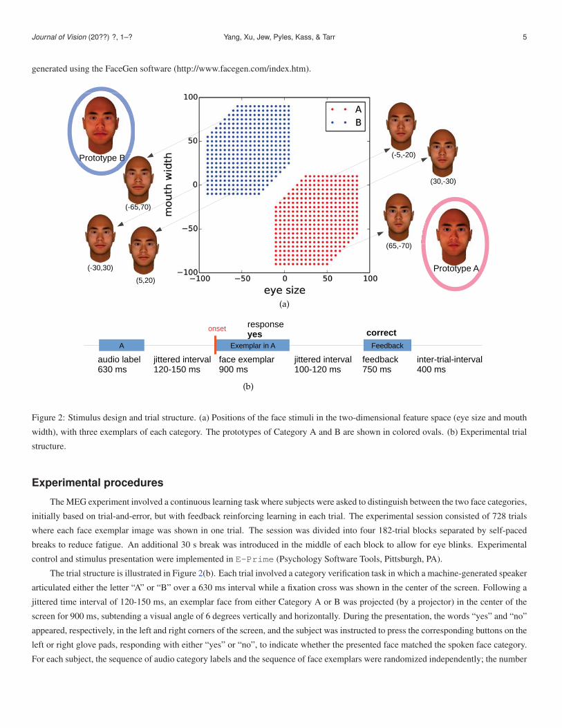
Figure 2: Stimulus design and trial structure. (a) Positions of the face stimuli in the two-dimensional feature space (eye size and mouth

width), with three exemplars of each category. The prototypes of Category A and B are shown in colored ovals. (b) Experimental trial

structure.

Experimental procedures

The MEG experiment involved a continuous learning task where subjects were asked to distinguish between the two face categories,

initially based on trial-and-error, but with feedback reinforcing learning in each trial. The experimental session consisted of 728 trials

where each face exemplar image was shown in one trial. The session was divided into four 182-trial blocks separated by self-paced

breaks to reduce fatigue. An additional 30 s break was introduced in the middle of each block to allow for eye blinks. Experimental

control and stimulus presentation were implemented in E-Prime (Psychology Software Tools, Pittsburgh, PA).

The trial structure is illustrated in Figure 2(b). Each trial involved a category verification task in which a machine-generated speaker

articulated either the letter “A” or “B” over a 630 ms interval while a fixation cross was shown in the center of the screen. Following a

jittered time interval of 120-150 ms, an exemplar face from either Category A or B was projected (by a projector) in the center of the

screen for 900 ms, subtending a visual angle of 6 degrees vertically and horizontally. During the presentation, the words “yes” and “no”

appeared, respectively, in the left and right corners of the screen, and the subject was instructed to press the corresponding buttons on the

left or right glove pads, responding with either “yes” or “no”, to indicate whether the presented face matched the spoken face category.

For each subject, the sequence of audio category labels and the sequence of face exemplars were randomized independently; the number


of “A”s and “B”s in both the audio sequence and the true category label sequence were maintained to be equal within every 20 trials. In

addition, the left or right positions of “yes”s and “no”s were counterbalanced across subjects. This design dissociated the particular left

or right motor responses from the true category labels of individual faces. Following the presentation of the face, a fixation cross was

shown across a jittered time interval of 100-120 ms. Feedback was then provided in the form of centered text for 750 ms, informing the

subject as to whether their response was correct, incorrect, or failed to occur within the given deadline (respectively, “correct,” “wrong,”

or “too slow”). Feedback was followed by an inter-trial-interval of 400 ms leading to the next trial. To encourage learning, a small

incremental reward scheme was used in which subjects additionally received $3, $5, or $7 if their average categorization accuracy in

Blocks 2, 3, and 4 exceeded 70%, 80%, and 90% respectively.

To define spatial face-sensitive regions (via source localization) for each subject, a separate functional localizer was run during the

MEG session. Similar to fMRI functional localizers (Grill-Spector, Kourtzi, & Kanwisher, 2001; Pyles et al., 2013), subjects viewed

color images of four categories: faces, everyday objects, houses and scrambled objects, and performed a one-back task in which they

responded whenever the same image was repeated across two sequential presentations. Images subtended a visual angle of 6 degrees

vertically and horizontally. Each category was presented in 16-trial groups, and each trial included an image from the current category,

presented for 800 ms with a 200 ms inter-trial-interval. A run consisted of 12 groups (3 groups x 4 category conditions) with 6 s fixations

between groups. Each subject participated in 4 runs, yielding 192 trials per a category.

Data acquisition and preprocessing

MEG. MEG signals were recorded using a 306-channel whole-head MEG system (Elekta Neuromag, Helsinki, Finland) at the

Brain Mapping Center at the University of Pittsburgh, while subjects performed the face category learning task and the one-back

functional localizer task in an electromagnetically shielded room. The MEG system had 102 triplets, each consisting of a magnetometer

and two perpendicular gradiometers. The data were acquired at 1 kHz, high-pass filtered at 0.1 Hz and low-pass filtered at 330 Hz.

Electrooculogram (EOG) was monitored by recording the differential electric potentials above and below the left eye, and lateral to both

eyes. Electrocardiography (ECG) was recorded by placing two additional electrodes above the chest. The EOG and ECG recordings

captured eye blinks and heartbeats, so that these artifacts could be removed from the MEG recordings afterwards. Four head position

indicator coils were placed on the subject’s scalp to record the position of the head in relation to the MEG helmet. Empty room MEG

data were also recorded in the same session, and used to estimate the covariance matrix of the sensor noise.

The MEG data in the face category learning experiment were preprocessed using MNE/MNE-python (Gramfort et al., 2013, 2014)

in the following steps. (1) The raw data were filtered with a 1-110 Hz bandpass filter, and then with a notch filter at 60 Hz to reduce the

power-line interference. (2) Temporal signal-space separation (tSSS) (Taulu & Simola, 2006), implemented in the MaxFilter software

provided by Elekta, was applied to the filtered data. This step further removed the noise from outside the MEG helmet. (3) Independent

component analysis (ICA) was used to decompose the MEG data into multiple components, and the components that were highly

correlated with eye blinks and heartbeats recorded by EOG and ECG were removed, via a default script in MNE-python. The ECG

and EOG data for one subject (s4) were corrupted; therefore the ICA artifact removal was not run for s4. (4) For each trial in the face

category learning experiment, the MEG data in -140-560 ms (with 0 being the stimulus onset) were used in the analyses. The signal-

space projection (SSP) method in MNE/MNE-python was further applied, where a low-dimensional linear subspace characterizing the

empty room noise was constructed, and the projection onto this subspace was removed from the MEG data. Finally, for each sensor,

trial, and subject, the mean of the baseline time window (-140 ms to -40 ms) was subtracted at each time point 2.

For the regression analysis below, the trial-by-trial MEG data were down-sampled at a 100 Hz sampling rate to reduce computa-

tional cost; for the discriminant analysis below, the trial-by-trial MEG data were smoothed with a 50 ms Hanning window to further

reduce high-frequency noise, and then down-sampled at the 100 Hz sampling rate.

The preprocessing of the functional localizer MEG data differed from the above procedure in the following ways3: (1) The data

were bandpass-filtered at 0.1 to 50 Hz; (2) tSSS was not applied; (3) principal component analysis instead of ICA was used to remove


artifacts such as eye blinks or movements; (4) any trials that showed EOG or ECG activities that were three standard deviations away

from the trial mean at any time point were discarded; (5) the baseline window was defined as -120 to 0 ms, and the data were binned

into 10 ms windows instead of down-sampling.

MRI. A structural magnetic resonance imaging (MRI) scan was acquired for each subject at the Scientific Imaging and Brain

Research Center at Carnegie Mellon University (Siemens Verio 3T, T1-weighted MPRAGE sequence, 1 × 1 × 1 mm, 176 sagittal

slices, TR = 2300 ms, TI= 900 ms, FA = 9 degrees, GRAPPA = 2). The cortical surface was reconstructed using Freesurfer

(http://surfer.nmr.mgh.harvard.edu/) (Dale, Fischl, & Sereno, 1999). The source space was defined as 6000 to 7000 discrete source

points almost evenly distributed on the bi-hemispheric cortical surfaces, with 7 mm separation on average, using the MNE/MNE-python

software. Each source point represented a current dipole (due to local neural activity) that was perpendicular to the cortical surface.

Regions of interest (ROIs)

The face-sensitive regions (regions of interest or ROIs) were defined in the source space using the functional localizer MEG data

for each subject. First, a time window of interest was defined in the following way. Trial-by-trial MEG sensor data were separated

based on the stimulus category, face or object. PCA-Hotelling tests (described below) preserving 99% variance were run on the

data from 102 magnetometer sensors, binned for every 10 ms from 0-400 ms, to examine whether the mean multivariate responses to

faces and to objects were statistically different in each bin. A window with 20 ms on both sides flanking around the lowest p-values

within 100-300 ms were defined as the time window of interest for each subject — these windows were at 180 ms on average, which

corresponded to the M/N170. Secondly, for each trial and for each of the 306 sensors, the MEG data within the time window of interest

were averaged, such that each trial was represented by a 306×1 vector. The minimum-norm estimate (MNE, Hamalainen & Ilmoniemi,

1994) of the source activity was obtained using these vectors. Thirdly, a “searchlight” Hotelling’s T-squared test (see below) was run

on the source activity for each source point and its two closest neighbors. The p-values of these tests reflected how much the three

grouped source points discriminated images of faces and objects. To focus on the face-sensitive regions commonly reported in the

fMRI literature, the searchlight procedure was anatomically bounded in regions of fusiform, lateraloccipital, superior temporal, inferior

frontal and orbitofrontal gyri as defined by Freesurfer’s parcellation. Finally, a threshold of p < 0.001 was applied to retrieve

those contiguous clusters that showed significant discriminability between faces and objects. Isolated small groups of source points

were manually removed. This procedure yielded 11 ROIs within the bilateral inferior occipital gyri (IOG), bilateral middle fusiform

(mFUS) gyri, bilateral anterior inferior temporal lobes (aIT), bilateral superior temporal areas (ST), bilateral inferior frontal gyri (IFG)

and the right orbitofrontal cortex (OFC). The identified superior temporal regions (ST) were roughly within the superior temporal sulci

or the superior temporal gyri, which were in the vicinity of the face-sensitive area in the posterior superior temporal sulcus (STS) in the

literature (Ishai, 2008). See Figure 4 and Figure 7 for illustration of the ROIs in one subject (s8). See Table 1 for details of the ROIs in

each subject.

Behavioral learning curves

To better characterize the dynamics of behavioral learning during the experiment, we derived behavioral learning curves for each

subject individually. Specifically, during each subject’s learning session, we measured a binary behavioral response after each trial

(1 for “correct” and 0 for “incorrect/too slow”). These binary observations can be viewed as Bernoulli outcomes from an underlying

real-valued accuracy rate, which varied with the trial index. To characterize the behavioral accuracy rate as a function of the trial index,

we expressed the rate as a linear combination of Legendre polynomials of order 5. Using this framework, a logistic regression model

was used to estimate the linear coefficients for each subject, and thus to reconstruct the function, which we refer to as the behavioral

learning curve. Observations from all the 728 trials were used. Individual subjects may have different learning rates for the two

face categories; thereby interaction terms between face categories and the Legendre basis were also included in the design matrix of

the logistic regression. As a consequence of this interaction, separate learning curves were estimated for each category. Note that one


IOG L IOG R mFUS L mFUS R aIT L aIT R ST L ST R IFG L IFG R OFC R

s1 20 18 13 68 5 17 0 10 7 7 3

s2 3 20 0 38 0 0 0 9 3 3 3

s3 20 21 44 50 6 0 5 3 19 0 0

s4 20 19 54 55 0 0 17 12 3 10 0

s5 18 14 25 43 7 0 3 0 16 0 0

s6 0 0 40 19 17 0 9 0 11 4 0

s7 0 20 46 28 0 9 0 14 0 6 0

s8 14 23 37 47 5 12 6 18 0 12 3

s10 19 14 40 19 0 0 0 13 7 19 0

nsubj 7 8 8 9 5 3 5 7 7 7 3

Table 1: Number of source points in each face-sensitive ROI for each subject. “0” indicates that the ROI was absent in the corresponding

subject. The suffixes “ L” and “ R” indicate that the ROI was in the left or the right hemisphere. nsubj in the last row indicates the

number of subjects for whom the ROI was found.

subject (s9) showed nearly flat behavioral learning curves for both categories (i.e., failed to learn) and was therefore excluded from

further data analysis.

Source localization

According to Maxwell’s equations, at each time point, the MEG sensor data can be approximated by a linear transformation of

the source signals plus sensor noise (Hamalainen et al., 1993). The source localization problem is essentially solving the inverse of

this linear transformation. In this experiment, the linear operator that projected source signals to the sensor space (also known as the

forward matrix) for each subject was computed using the boundary element model in the MNE software, according to the position

and shape of the head and the positions of the MEG sensors. Because the head position was recorded at the beginning of each half-block,

we computed a forward matrix for each of the 8 half-blocks, to correct for run-to-run head movement. The covariance of the sensor

noise was estimated from empty room recordings, and used for the source localization methods below.

The minimum norm estimate (MNE, Hamalainen & Ilmoniemi, 1994), which constrains the inverse problem by penalizing the sum

of squares (i.e., squared L2 norms) of the source solution, was used to obtain the source estimates in the functional localizer experiment

to define the face-sensitive ROIs. In the regression and discriminant analyses of the face category learning experiment (discussed below),

a variation of the MNE, the dynamic statistical parametric mapping (dSPM) method (Dale et al., 2000), was used to estimate the source

space activity for each trial separately. As an improvement of the MNE method, dSPM normalizes the estimated source activities to

dimensionless variables, and thus reduces the bias towards superficial source points in MNE. Both MNE and dSPM were implemented

in MNE/MNE-python with the regularization parameter set to 1.0.

The dSPM method is easy to implement and widely used. However, it does not emphasize the face-sensitive ROIs, nor does it

encourage temporal smoothness. Moreover, our goal was to investigate how much trial-by-trial neural responses in the source space were

correlated with behavioral learning curves; with dSPM solutions, one needs to do an additional regression step to quantify the correlation.

Possible localization errors in the dSPM solutions may yield inaccurate regression results. In this context, for the source-space regression

analysis, we also used our newly developed short-time Fourier transform regression model (STFT-R) in Yang et al., 2014. STFT-R uses

a time-frequency decomposition to represent source activities and embeds a linear regression of each time-frequency component against

trial-by-trial regressors (i.e., the behavioral learning curve here). In this one-step framework, the regression coefficients are solved in the

source localization step, with constraints that emphasize the ROIs and encourage sparsity over the time-frequency components for each


source point. Due to such sparsity, the estimated regression coefficients (transformed back to the time domain) are temporally smooth

and concentrated around time windows of interest (e.g., time windows after the baseline window); therefore they are easier to interpret

than those derived from MNE/dSPM solutions. Details of STFT-R are described in Yang et al., 2014, and the Python code is available at

https://github.com/YingYang/STFT R git repo. For the short-time Fourier transform in our current experiment, 160 ms

time windows and 40 ms steps were used, resulting in frequencies from 0 to 50 Hz, spaced by 6.25 Hz, according to the 100 Hz sampling

rate. The MEG data were split into two halves (odd and even trials). The first half was used in learning the sparse structures in STFT-R;

the second half was used to obtain estimates of the regression coefficients, constrained on the sparse structure, with penalization of their

squared L2 norms to reduce the biases generated by the sparsity constraints. The penalization parameters were determined via a 2-fold

cross-validation, by minimizing the mean squared errors of the predicted sensor data.

Regression analysis

For sensor space regression in the time domain, we ran, at each time point, for each sensor and each subject, a separate regression

against the behavioral learning curve using trials in each face category. With only one regressor in this analysis, we fitted two coefficients

— a slope and an intercept. Interested in the correlation with the behavioral learning curve, we focused on the slope coefficient. Signif-

icantly non-zero slope coefficients indicate significant correlations between the MEG data and the behavioral learning curve. P -values

of two-sided t-tests of the slope coefficients were obtained, indicating the degree to which the coefficients were significantly different

from zero. We took the negative logarithms with base 10 of these p-values (− log10(p)) as statistics and call them correlation

significance hereafter.

For regression analyses in the face-sensitive ROIs in the source space, for trials corresponding to each face category separately,

the STFT-R model produced regression coefficients of the time-frequency components of each source point. Inverse STFT was used to

transform the slope coefficients in the time-frequency domain to slope coefficients at each time point (which we call“slope coefficient

time series”), for each source point. A permutation test, where the trial correspondence with the behavioral learning curve was randomly

permuted, was used to test whether the slope coefficients were significantly non-zero, for each face category and each subject. This

permutation was only applied in the second half of the split trials. That is, in each permutation, the coefficients were obtained with

penalization of their squared L2 norms, on the permuted second half of the trials, but constrained on the non-zero structure learned

from first half trials of the original data. Note that each source point represented an electric current dipole perpendicular to the cortical

surface; signs of the source activity only indicated the directions of the dipoles. In other words, positive and negative slope coefficients

with the same magnitudes were equally meaningful. Therefore when summarizing the coefficients in an ROI, we averaged the squares of

the coefficients across source points in the ROI. The p-value of the permutation test was defined as the proportion of permutations where

such an averaged square was greater than the non-permuted counterpart. Again, − log10(p)s were used as the summarizing statistics,

reflecting the significance of correlation with learning. Similarly, for the dSPM solutions corresponding to each face category, we ran a

regression for each source point at each time point within the ROIs, and obtained − log10(p)s using the same permutation tests. Note

that there was no data-split for the dSPM solutions, so the number of trials was twice of that in the STFT-R.

Discriminant analysis

To test whether multivariate neural responses from multiple sensors or source points were able to discriminate between the two face

categories, Hotelling’s two-sample T -squared tests were run on the multivariate responses at each time point, for the smoothed data.

Let yr ∈ Rn be the response of n sensors or source points at a certain time point, in the rth trial. Let A and B denote the set of trials

corresponding to Categories A and B, and qA, qB be the number of trials in each category. The Hotelling’s T -squared was computed in

the following way. First, the sample mean for each category was obtained:

yA =1

qA

∑

r∈A

yr yB =1

qB

∑

r∈B

yr


Secondly, a common covariance matrix for both categories was estimated as:

W =

∑r∈A(yr − yA)(yr − yA)

T +∑

i∈B(yr − yB)(yr − yB)T

qA + qB − 2

Thirdly, the test statistic, T -squared, was defined as:

t2 =(yA − yB)

TW−1(yA − yB)

1/qA + 1/qB

Under the null hypothesis that the means of the two categories were the same, t2 was related to an F -distribution:

qA + qb − n− 1

n(qA + qB − 2)t2 ∼ F(n, qA + qB − n− 1)

from which p-values were obtained. Similarly as in the regression analysis, negative logarithms with base 10 of the p-values (− log10(p))

of the Hotelling’s T -squared tests, which we term discriminability, were used as statistics to reflect whether neural responses

were able to distinguish between the two face categories.

We applied the tests above to both sensor recordings and the dSPM source solutions within each ROI, at each time point. Note

that for source-space analysis, this is a two-step approach. Presumably, a one-step approach combining discriminability tests and source

localization will yield more accurate results. However, given that such models have not been developed, we used the two-step approach

with dSPM solutions here. For a large number of sensors or source points, there might not be a sufficient number of trials to estimate the

covariance matrix. Prior to applying Hotelling’s T -squared tests, two different approaches to dimensionality reduction were separately

applied to source space analysis and sensor space analysis. First, for source points within an ROI, whose responses were often highly

correlated, principal component analysis was used discarding the category labels, and then only the projections onto the first several

principal components preserving 99% variance were used in the Hotelling’s T -squared tests. We call this approach PCA-Hotelling.

Second, in sensor space, we observed that the PCA-Hotelling procedure did not perform well on the 306-dimensional sensor data,

possibly because the number of dimensions required to capture 99% variance was still large compared with the number of trials. Instead,

we used a different approach referred to as split-Hotelling: the trials were split into two parts, and a univariate two-sample t-test,

which examined whether the sensor responses for the two categories were different, was run on each sensor for the first half of the trials.

The top 20 sensors with the lowest p-values were selected. For the second half of the trials, Hotelling’s T -squared test was only applied

on the selected sensors, where the multivariate sensor data were normalized (z-scored) such that each dimension had the same variance.

This split was independently run multiple times, and negative logarithms with base 10 of the p-values (− log10(p)) of the splits were

averaged as the final statistics.

Tests of aggregated statistics across subjects

After obtaining the statistics above (correlation significance and discriminability) for individual subjects, we ran hypothesis tests

at group level. Below, we first introduce how confidence intervals of statistics averaged across subjects were computed, and then

introduce two different group-level tests. The first, permutation-excursion test was applied when statistics from all subject

were available. The second, Fisher’s method, was applied in source space analysis, where not every ROI was detected in every

subject. This method is good at detecting effects when the number of subjects is small, which was the case for several ROIs that were

identified in only a few subjects (see the last row of Table 1 for aIT L, aIT R, ST L and OFC R).

Percentile confidence intervals The statistics such as − log10(p) obtained from the analyses above were pri-

marily time series. To obtain group-level statistics at each time point we averaged these time series across subjects. To visualize the

uncertainty of the average, bootstrapping – random re-sampling of the time series at the subject level with replacement – was used, and

percentile confidence intervals (Wasserman, 2010) were obtained.


Permutation-excursion tests When examining whether time series of statistics are significantly different from the

null hypothesis, it is necessary to correct for multiple comparisons across different time points. Here, permutation-excursion tests (Maris

& Oostenveld, 2007; Xu, Sudre, Wang, Weber, & Kass, 2011), were used to control the family-wise error rate and obtain a global p-value

for time windows. In a one-sided test to examine whether some statistics are significantly larger than the null, we first identify clusters

of continuous time points where the statistics are above a threshold, and then take the sum within each of these clusters. Similarly, in

each permutation, the statistics of permuted data are thresholded, and summed for each of the detected clusters. The global p-value for a

cluster in the original, non-permuted case, is then defined as the proportion of permutations, where the largest summed statistics among

all detected clusters is greater than the summed statistics in that cluster from the non-permuted data.

In the regression and discriminant analyses in the sensor space, we tested whether the averaged − log10(p) time series across

subjects were significantly greater than baseline. This was accomplished by subtracting the averaged − log10(p) across time points in

the baseline window (-140 to -40 ms) from the − log10(p) time series, individually for each subject, and a t-test was used to examine if

the group means of these differences were significantly above zero at any time windows. Here the testing statistics for the excursion were

the t-statistics across subjects at each time point, and each permutation was implemented by assigning a random sign to the difference

time series for each subject. This test, which we refer to as permutation-excursion t-test hereafter, was implemented in

MNE-python, where the number of permutations was set to 1024, and the threshold of the t-statistics was equivalent to an uncorrected

p ≤ 0.05.

Fisher’s method For each ROI in the source space, we used Fisher’s method to combine p-values from regression analysis

or discriminant analysis across individual subjects. Let {pi}, i = 1 . . . ,K denote p-values of K independent tests (in K subjects).

Fisher’s method tests against the hypothesis that for each individual subject the null hypothesis is true. Under the null, −2∑K

i=1 log pi

has a χ22K distribution with 2K degrees of freedom, and a combined p-value is obtained based on the χ2

2K null distribution. As the

individual p-values were obtained for each time point, Fisher’s method was applied for each time point as well. Subsequently, to

correct for multiple comparisons at all time points and all ROIs, we applied Bonferroni criterion to control the family-wise error rate.

Considering such correction may be overly conservative, we also applied the Benjamini-Hochberg-Yekutieli procedure, which controlled

the false discovery rate under any dependency structure of the combined p-values at different time points and ROIs (see Theorem 1.3 in

Benjamini & Yekutieli, 2001 and Genovese, Lazar, & Nichols, 2002).

Results

We first present estimated behavioral learning curves; then, in the sensor space and in the source space (in the face-sensitive

ROIs), we connect behavioral learning curves to changes in neural activity over time, thereby revealing the neural correlates of learning.

Finally, we present a complementary discriminant analysis both in the sensor space and in the face-sensitive ROIs, in order to connect

the patterns of correlation with learning to the patterns of discriminability between the two face categories.

Fitting behavioral learning curves

As discussed, one subject showed no evidence of learning and was excluded from further analyses. In contrast, all nine other

subjects learned the face categorization task successfully. Based on the trial-by-trial behavioral responses (“correct” or “incorrect/too

slow”), we estimated the behavioral learning curves for each subject using a logistic regression on Legendre polynomial basis functions.

A face category factor was also included in the regression in order to fit the learning curves of the two categories separately. Figure 3(a)

shows the learning curve first averaged across the two categories, then averaged across the nine included subjects. The blue band shows

95% percentile confidence intervals, bootstrapped at subject-level, with Bonferroni correction for 728 trials (i.e., the

point-wise confidence range covers an interval of (2.5%/728, 1 − 2.5%/728)). The averaged accuracy rose from near 50% (chance)

to about 80% in the first 500 trials. Since the learning curves were steeper in the earlier trials, we used only the first 500 trials in the

following regression analysis to estimate learning effects. Figure S1 in the supplementary materials shows the fitted curves for each face


category and each individual subject. All nine subjects showed increasing trends and reached at least around 70% accuracy near the

500th trials.

(a) (b)

(c)

Figure 3: Regression against the behavioral learning curves in the sensor space. (a) The overall learning curve averaged across two

categories and across nine subjects. The blue band shows 95% confidence intervals. (b) The correlation significance

(− log10(p) of the regression analysis) averaged across all 306 sensors and two face categories, further averaged across subjects. The

blue band shows 95% confidence intervals; the red area indicates a window where the group average were significantly higher than the

baseline (-140 to -40 ms), with the corrected p-value marked (right sided permutation-excursion t-test, 9 subjects). (c) Heat

maps of averaged correlation significance (− log10(p) of the regression analysis) across both face categories and all subjects, further

averaged in 60 ms windows centering at the labeled time points, on sensor topology maps viewed from the top of the helmet, with the

upper end pointing to the anterior side.

Identifying the neural correlates of learning

To investigate the neural correlates of learning, we ran regression of trial-by-trial data against behavioral learning curves, first in

the MEG sensor space, and then in the source space within the face-sensitive ROIs. The sensor space results, which do not depend on

solutions to the source localization problem, can roughly demonstrate the temporal profile of correlation with learning, but not detailed

spatial localization. In contrast, the source space results provide higher spatial resolution and allow us to compare the learning profiles

in different ROIs within the face network. 4 5

Sensor space analysis

To identify the neural correlates of learning in MEG sensor recordings, we first regressed sensor data against the learning curves

for each subject, which are shown in Figure S1. The regression was run for each sensor at each time point. Observing that for some

subjects, the learning curves might be different between the two face categories, we ran the regression for the two categories separately.

For example, only trials in Category A were used in the regression against the learning curve for Category A. Since the learning curves

were steeper at the beginning, we only used the first 250 trials for each category (500 trials in total). To quantify the significance

of non-zero correlations between the MEG signals and behavioral learning curves, we computed the p-values of the regression slope

coefficients, and used − log10(p)s (correlation significance) as statistics to reflect the strength of the correlation effect with


learning.

To visualize the overall correlation effect across sensors, we averaged the correlation significance across both face categories and

then across all 306 sensors for each subject, resulting in nine time series of correlation significance for nine subjects. Figure 3(b) shows

the average of these time series across subjects, as well as 95% confidence intervals, bootstrapped at the subject-level, with Bonferroni

correction for 71 time points (i.e., the point-wise confidence range covers an interval of (2.5%/71, 1−2.5%/71)). Based on a right-sided

permutation-excursion t-test against the baseline (-140 to -40 ms), we observed a significant time window (p < 0.01) within 90-560 ms,

in which the correlation effect was predominant within 150-250 ms. To visualize which sensors contributed to this effect, in Figure 3(c)

we plotted the correlation significance averaged across categories and subjects, and then further averaged over 60 ms windows centering

at labeled time points on topology maps of sensors, viewed from the top of the MEG helmet. Again, we observed a high correlation

effect with learning roughly within 150-250 ms, and this effect was larger in the posterior sensors and the left and right temporal sensors,

which are close to the visual cortex in the occipital and temporal lobes.

Source space ROI analysis

The sensor space results demonstrated that the neural activity measured by MEG was correlated with behavioral learning. To

spatially pinpoint the correlation effect in the ROIs of the face network, we applied the one-step STFT-R model for regression analysis

in the source space. Similarly to our sensor space analysis, we only analyzed the first 250 trials for each category (i.e., the first 500 trials

in total), and because of the data-split paradigm in STFT-R, the effective number of trials we analyzed in each category was 125.

Additionally, we also ran a two-step regression analysis—obtaining dSPM source solutions for each trial and running regression

afterwards, which is along with the traditional pipeline of MEG source-space analysis (e.g. as in Xu et al., 2013). Note that unlike the

STFT-R model, the dSPM source localization did not emphasize the face-sensitive ROIs, nor did it encourage sparsity in the spatial and

time-frequency domains; the correlation effect identified by the two-step method could be spatially more spread out and temporally less

smooth than that by STFT-R. Another difference was that we were able to use all 250 trials for each category, because there was no data

split in the two-step method.

With both STFT-R and the two-step method, we used permutation tests to examine whether the slope coefficients in each ROI were

non-zero–we averaged the squares of slope coefficients across source points in each ROI at each time point, and compared them with

permuted counterparts. Forty permutations of the trial indices in the regressor (i.e., behavioral learning curves) were run for each subject

and each face category independently. We used Fisher’s method to combine the permutation p-values between the two categories, at

each time point in each ROI of each subject. We computed correlation significance, − log10 of the combined p-values,

which indicate whether, for at least one category, the slope coefficients were significantly above chance. Individual times series of

correlation significance by STFT-R are plotted in Figure S2 in the supplementary materials. We then used Fisher’s method to further

combine individual p-values across subjects for each ROI at each time point. Figure 4 shows the − log10 of these group-level p-values

by STFT-R. The red solid lines indicate a significant threshold at level 0.05, with Bonferroni correction for multiple comparisons at

71 time points × 11 ROIs (781 comparisons in total); the red dashdot lines indicate a threshold where the false discovery rate was

controlled at 0.05, by the Benjamini-Hochberg-Yekutieli procedure.

From the STFT-R results in Figure 4, we observed that in the ventral pathway, the − log10 of the combined p-values passed the

Bonferroni threshold (red solid lines) in the right IOG and bilateral mFUS in time windows roughly within 150-250 ms, and in the

right mFUS in a later (post 300 ms) time window; these results indicate that in these ROIs within the aforementioned time windows,

neural activity was significantly correlated with behavioral learning, at least for some of the subjects, where the family-wise error rate

was smaller than 0.05. Using a less conservative threshold, where the false discovery rate was controlled at 0.05 (red dashdot lines),

we observed significant correlations with learning in bilateral IOG, bilateral mFUS and the left aIT in time windows roughly within

150-250 ms, and in IOG and mFUS in later (post 300 ms) time windows as well. However, with STFT-R, in the non-ventral ROIs (ST

and the two prefrontal regions, IFG and OFC), we did not observe significant correlation with learning using either of the thresholds.


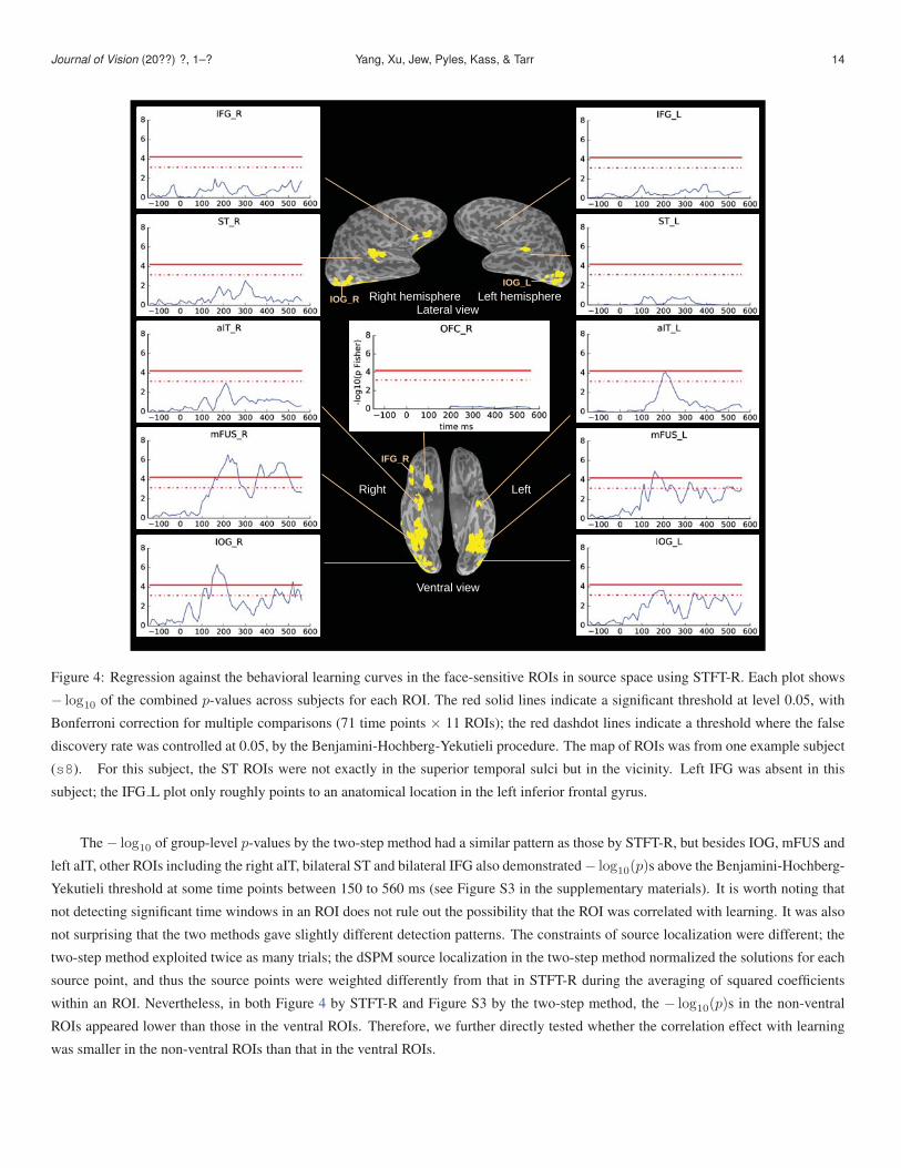
Figure 4: Regression against the behavioral learning curves in the face-sensitive ROIs in source space using STFT-R. Each plot shows

− log10 of the combined p-values across subjects for each ROI. The red solid lines indicate a significant threshold at level 0.05, with

Bonferroni correction for multiple comparisons (71 time points × 11 ROIs); the red dashdot lines indicate a threshold where the false

discovery rate was controlled at 0.05, by the Benjamini-Hochberg-Yekutieli procedure. The map of ROIs was from one example subject

(s8). For this subject, the ST ROIs were not exactly in the superior temporal sulci but in the vicinity. Left IFG was absent in this

subject; the IFG L plot only roughly points to an anatomical location in the left inferior frontal gyrus.

The − log10 of group-level p-values by the two-step method had a similar pattern as those by STFT-R, but besides IOG, mFUS and

left aIT, other ROIs including the right aIT, bilateral ST and bilateral IFG also demonstrated − log10(p)s above the Benjamini-Hochberg-

Yekutieli threshold at some time points between 150 to 560 ms (see Figure S3 in the supplementary materials). It is worth noting that

not detecting significant time windows in an ROI does not rule out the possibility that the ROI was correlated with learning. It was also

not surprising that the two methods gave slightly different detection patterns. The constraints of source localization were different; the

two-step method exploited twice as many trials; the dSPM source localization in the two-step method normalized the solutions for each

source point, and thus the source points were weighted differently from that in STFT-R during the averaging of squared coefficients

within an ROI. Nevertheless, in both Figure 4 by STFT-R and Figure S3 by the two-step method, the − log10(p)s in the non-ventral

ROIs appeared lower than those in the ventral ROIs. Therefore, we further directly tested whether the correlation effect with learning

was smaller in the non-ventral ROIs than that in the ventral ROIs.


We merged the ventral ROIs (bilateral IOG, mFUS and aIT) into one group, and the non-ventral ROIs (bilateral ST, IFG and the

right OFC) into another group. In this way, each subject had a merged ventral group and a merged non-ventral group; therefore we

were able to use all nine subjects in the analysis for the two groups of ROIs. Using STFT-R, we ran the permutation tests for each

merged group for each individual subject in the same way as above, and took the difference of the correlation significance (− log10 of

the combined p-values for two categories) between the non-ventral group and the ventral group, at each time point, for each subject.

We applied permutation-excursion t-tests to examine whether the average of the computed differences across subjects was

non-zero at certain time points, and found that the averaged difference was significantly negative from roughly 170 to 250 ms (Figure 5);

that is, the correlation effects with learning were significantly smaller (p < 0.05) in the non-ventral ROIs than in the ventral ROIs. In

contrast, we did not detect significant positive differences. Such a direct comparison suggests that the correlation effect with learning in

the ventral ROIs was stronger than that in the non-ventral ROIs.

Figure 5: The averaged difference of correlation significance between the non-ventral group of ROIs (other) and the ventral group of

ROIs (ventral), using STFT-R. The blue band shows 95% confidence intervals; the red area shows the significant time window from

a two-sided permutation-excursion t-test on the nine subjects, with the p-value marked.

Discriminant analysis

In the analysis presented above, we localized the neural correlates of learning in the majority of the ROIs. The strongest effects

were found in the ventral ROIs, mainly within 150 to 250 ms, but also in later, post 300 ms time windows in IOG and mFUS. As a

complementary analysis, we also examined whether these ROIs encoded information for face categorization in similar time windows.

We obtained a spatio-temporal profile to quantify how effectively each ROI discriminated between the two face categories, and then

compared this discriminability profile with the learning correlation profile. This discriminant analysis was run on the MEG sensor data

first, and then on the dSPM source solutions in the ROIs, testing whether the neural representations of the two face categories were

different. To achieve higher power in these tests, all 728 trials in the entire learning session were used.

Sensor space analysis

We ran the split-Hotelling tests on the 306-dimensional sensor data at each time point and used − log10 of p-values of the

tests to index the discriminability of the neural activities. Figure 6 shows the averaged discriminability across subjects, using all 728 tri-

als. We tested whether the averaged discriminability was greater than the baseline (-140 to -40 ms), using the permutation-excursion

t-test. We observed significant discriminability (p < 0.01) starting from about 140 ms and lasting up to about 560 ms, which indicates

that the MEG signals carried information that discriminated between the two categories beginning at about 140 ms post stimulus onset.

In contrast with the correlation significance in the sensor space (Figure 3(b)), which had a single peak near 200 ms, the discriminability

depicted in Figure 6 appeared to have multiple peaks, and was stronger in a later time window post 300 ms. This comparison in the tem-


poral domain suggests that there are both early and late temporal components related to the neural representations of the two categories,

and the early component could be more correlated with learning than the later component. However, more detailed comparisons require

directly contrasting the spatio-temporal profiles of discriminability and learning effects; consequently, we move to source space in the

next analyses.

Figure 6: Discriminant analysis of the sensor data: averaged − log10(p) across subjects in split-Hotelling tests over 728 trials.

The blue band shows 95% confidence intervals; the red area shows the significant time window by the permutation-excursion t-test,

with the p-values marked.

Source space ROI analysis

To obtain a spatio-temporal discriminability profile for the face-sensitive ROIs, we applied the PCA-Hotelling procedure to

the dSPM source solutions in each ROI using all 728 trials. The discriminability, at each time point for each ROI in each subject, was

quantified by − log10 of the p-values from the PCA-Hotelling procedure and is plotted in Figure S4 in the supplementary materials.

We then used Fisher’s method to combine the PCA-Hotelling p-values across subjects at each time point and in each ROI, and

plotted the − log10 of the combined p-values in Figure 7. The green solid lines indicate a significant threshold at level 0.05, with

Bonferroni correction for multiple comparisons (71 time points × 11 ROIs); the green dashdot lines indicate a threshold where the false

discovery rate was controlled at 0.05, by the Benjamini-Hochberg-Yekutieli procedure.

In Figure 7, the majority of the ROIs showed significant discriminability between categories. Only the right aIT and right OFC

did not pass the Bonferroni threshold at any time windows, and only the right OFC did not pass the Benjamini-Hochberg-Yekutieli

threshold for false discovery rate control. These results indicate that neural signals in the majority of the ROIs significantly discriminated

between the two face categories for at least one subject. More interestingly, the prefrontal regions (bilateral IFG) and the higher-level

ventral region (bilateral aIT) only demonstrated the significant discriminability in later (post 300 ms) time windows. The bilateral

ST also demonstrated a similar pattern of late discriminability, although there appeared to be some earlier (pre 300 ms) time points

where the − log10(p) was close to the Benjamini-Hochberg-Yekutieli threshold. In contrast to the ROIs above, the lower- and mid-

level ROIs within the ventral pathway exhibited a different pattern featuring both early and late discriminability—bilateral IOG and

mFUS both exhibited late (post 300 ms) − log10(p) above the Bonferroni threshold; moreover, in pre 300 ms time windows, the left

mFUS and bilateral IOG exhibited − log10(p) above the Bonferroni threshold, and the right mFUS exhibited − log10(p) above the less

conservative Benjamini-Hochberg-Yekutieli threshold near 200 ms and 280 ms. In addition, the profile of discriminability within ventral

ROIs appears to be consistent with the hypothesis that IOG, mFUS and aIT follow a lower- to higher-level hierarchical organization, as


the initial increases of discriminability roughly demonstrated an early-to-late pattern along the IOG-mFUS-aIT direction, especially in

the right hemisphere.

Figure 7: Discriminability analysis in face-sensitive ROIs. Each plot shows − log10 of combined p-values across subjects for each

ROI. The green solid lines indicate a significant threshold at level 0.05, with Bonferroni correction for multiple comparisons (71 time

points × 11 ROIs); the green dashdot lines indicate a threshold where the false discovery rate was controlled at 0.05, by the Benjamini-

Hochberg-Yekutieli procedure. The map of ROIs is from subject s8 (as in Figure 4).

Comparing the discriminability profile shown in Figure 7 to the correlation profile with learning shown in Figure 4, we note that the

ventral ROIs that exhibited earlier discriminability, that is, IOG and mFUS, were also the ROIs that exhibited a strong correlation effect

with learning. Although the time course of discriminability did not precisely align with the time course of correlation with learning

at individual level (Figure S2 and Figure S4), the overall co-localization suggests that these ventral ROIs — known to process visual

features of faces — seem likely to underlie face learning, particularly during the early processing window of 150-250 ms. In addition,

it is possible that IOG and mFUS are also involved in learning during a later window of post 300 ms. In contrast, non-ventral regions of

the face network expressed facial category discriminability mostly post 300 ms and, moreover, had a less strong correlation effect with

learning than the ventral ROIs. In sum, our results suggest that early and recurring temporal components arising from ventral regions in

the face network are critically involved in learning new faces.


Discussion

Connections to previously-identified temporal signatures of face processing

In contrast to traditional EEG studies that focus on event related potentials (ERPs), our analysis of MEG sensor space data was

not constrained to only the peaks or latencies of specific event-related components. Instead, we analyzed the correlations of neural

activity with learning across the entire 0 to 560 ms window covering what might be construed as the outer bound for the feed-forward

perception of faces. Critically, this reasonably broad time window does not preclude some level of feedback in face processing. Using

this approach, we observed significant correlations with face learning ranging from about 90 ms to 560 ms. The effect of learning was

most apparent from roughly 150 to 250 ms, which corresponds to both the M/N170 and N250 time windows in the MEG/EEG literature.

The N250 component is often interpreted as an index of familiarity (Schweinberger, Huddy, & Burton, 2004; Tanaka et al., 2006; Pierce

et al., 2011; Barragan-Jason et al., 2015) or a temporal marker of general perceptual learning (Krigolson, Pierce, Holroyd, & Tanaka,

2009; Pierce et al., 2011; Xu et al., 2013). M/N170 is typically construed as a component reflecting face detection and individuation

(Liu et al., 2000). Recently, changes in both the M/N170 and the N250 components have been reported in face-related learning tasks

(Su et al., 2013; Itz et al., 2014) and in experiments involving repeated presentations of faces (Itier & Taylor, 2004). Barragan-Jason et

al., 2015 have also suggested facial familiarity effects may rely on rapid face processing indexed by M/N170, as well as later processing

indexed by N250. Our results support the involvement of both the M/N170 and the N250 in face learning, consistent with these previous

reports.

In our complimentary multivariate discriminant analysis, we observed that MEG sensor data significantly discriminated between

the two face categories as early as 140 ms, with continued discriminability occurring as late as 560 ms. This window of discriminability

included M/N170 but also N250, suggesting that both components encode information that can support face individuation. More broadly,

this observed facial category discriminability time window is also consistent with the 200 to 500 ms time window for face individuation

observed when using direct electrode recordings in the human fusiform gyrus (Ghuman et al., 2014).

Functional roles of face-sensitive ROIs during face learning

Although the M/N170 and N250 have been approximately localized to the fusiform gyrus (Deffke et al., 2007; Schweinberger

et al., 2004), our work directly describes a more comprehensive spatio-temporal profile over learning within the entire face network.

We observed stronger correlation effects with learning in the ventral visual ROIs than in the non-ventral ROIs. The ventral ROIs are

hypothesized to process the visual features of faces, whereas the non-ventral ROIs are hypothesized to process semantic information

or social information (Ishai, 2008; Nestor et al., 2008). In this context, our results are consistent with the hypothesis that learning new

faces is enabled primarily through visual processing.

The IOG, mFUS, and aIT along the ventral pathway have been hypothesized to process visual features in a hierarchical manner.

Although Jiang et al., 2011 challenged this view, their study used fMRI during face detection in noisy images, which cannot rule out

processes arising from top-down feedback induced by noisy stimuli. In our multivariate discriminant analysis of dSPM source solutions

across all trials in the learning session, we found significant discriminability between the two face categories, post 300 ms, in the

majority of face-sensitive ROIs. However, earlier significant discriminability was observed mainly in IOG and mFUS. We also observed

that the initial increases in discriminability appeared to be earlier in IOG than in mFUS in the right hemisphere (Figures 7 and S4).

Such a pattern is consistent with the hypothesis of an IOG→mFUS→aIT hierarchy, where information flows from the lower-level to

higher-level regions. Notably, the ROIs that exhibited earlier discriminability before 300 ms (IOG and mFUS) were also the brain

regions that showed strong correlation effects with behavioral learning, suggesting an important role for visual processing in learning

new faces. Additionally, IOG and mFUS also exhibited correlation with learning in post 300 ms, which could be due to feedback from

the higher-level regions that is modified by the learning process.

The early peaks of discriminability near 100 to 120 ms in IOG and the left mFUS were observed slightly later than the responses


typically seen in the early visual cortex at or before 100 ms (Bair, Cavanaugh, Smith, & Movshon, 2002; Cichy, Pantazis, & Oliva,

2014). Such early discriminability in IOG is likely based on visual information — derived from relatively small receptive fields —

passed from low-level visual areas (e.g., V1, V2, and V3). Under this view, we can hypothesize that early discriminability arises from

representations of local facial parts that contain diagnostic features (e.g., the mouth width and eye size in our design space in Figure 2).

However, it is difficult to test this hypothesis using only the temporal pattern of discriminability we observed here; IOG may receive

inputs from neurons whose receptive fields cover a wide range or even entire faces. We should also note that due to spatial correlations

in the forward transformation from the source space to the MEG sensor space, the reconstructed source solutions by the dSPM method

can be spatially blurred, and neural activity from nearby brain areas may be localized in face-sensitive ROIs. This methodological issue

increases the difficulty of determining the functional origins of the early discriminability.

Comparing discriminability in early and late stages of learning

Although several ROIs exhibited significant correlations with behavioral learning curves, when we directly compared the multi-

variate discriminability between early and late stages of the learning session (i.e., the first and the last 200 trials), we did not observe

significant changes in the face-sensitive ROIs. Figure S5 shows the difference in discriminability between the late stage and the early

stage of learning in both the IOG and mFUS, the ROIs that had strong correlation effects with behavioral learning curves. To increase

power, we averaged the discriminability across the corresponding bilateral regions. The green bands show 95% marginal intervals of

the difference in discriminability under the null hypothesis (i.e., zero difference), uncorrected for multiple comparisons, obtained from

500 permutations in which the trial labels for early and late stages were permuted. Using permutation-excursion tests,

which corrected for multiple comparisons, we did not find any windows where the averaged difference across subjects was significantly

non-zero at a level of 0.05, although there appeared to be a trend for IOG having an increase in discriminability near 220 ms, and mFUS

having a decrease near 200 ms as well as an increase near 350 ms.

To explore the possibility of more fine-grained learning effects, we also compared the discriminability in the first 100 trials to the

discriminability in the next 100 trials (from 100 to 200). However, this comparison did not detect any significant difference. Of course,

in light of the fact that statistical tests and the corrections for multiple comparisons are generally biased towards the null hypothesis,

our failure to detect any difference does not imply that there was not an actual difference in discriminability during different stages of

learning.

On one hand, these results may suggest that the general changes in the representations of both categories were measurably stronger

than any changes in the discriminant representation between the two categories. We speculate that face-sensitive brain regions are

already highly efficient in representing facial features (given the extensive experience all adults have had with faces); as such, any

changes in discriminability during learning of new faces are likely to be small and subtle, and, therefore, difficult to detect. On the other

hand, an empirically driven alternative explanation may be that learning occurred too quickly in our experiment, thereby reducing the

number of trials available to reliably estimate multivariate discriminability in the early learning stage. That is, if learning is very rapid,

we are likely to observe little difference in the estimated discriminability in the first 200 trials and the last 200 trials (or in the first 100

trials and the next 100 trials).

Difficulty of exemplars

In the design space illustrated in Figure 2 (i.e., the two-dimensional space of eye size and mouth width), the distance from each

exemplar to the decision boundary of the two categories varied by exemplar. More specifically, this means that the exemplars far from

the decision boundary (e.g., (-65,70)) could be easier to learn than the exemplars close to the decision boundary (e.g., (5,20)). In

an exploratory analysis of our behavioral data, we equally divided the exemplars in each category into two groups according to their

euclidean distances to the decision boundary, labelling the exemplars closer to the boundary as “easy” and the exemplars farther from the

boundary as “hard”. For the “easy” exemplars, the behavioral accuracy was higher in the majority of the subjects, and the learning curves


appeared steeper in the early stages of learning for 5 out of our 10 subjects. As such and not surprisingly, it is likely that behavioral

learning is somewhat dependent on the difficulty of the stimuli. In an additional exploratory analysis of the neural data, we regressed

the dSPM source solutions in the face-sensitive ROIs against both the behavioral learning curves and the difficulty of the exemplars6.

However, this analysis failed to detect any significant linear dependence for the neural data on the interaction between difficulty and

behavioral learning. Note that this does not mean that there were not any interaction effects; it is possible that the variations of difficulty

within our stimulus space were simply insufficient to detect an effect. In future work, it would be interesting to investigate how neural

learning dynamics vary with categorization difficulty, in particular, using a sufficiently complex stimulus set.

Issues and limitations

One important limitation of our study involves the fact that we did not collect neural responses for any untrained face stimuli. More

specifically, this lack of control with respect to the trained stimuli leaves open the question as to whether the changes we observed apply

to face representations more generally (e.g., there was a change in the neural code associated with all faces) or whether the changes

we observed were specific to the trained faces used in our experiment. An example of the former would be temporarily sharpened

representations across all known faces or the learning of features that support better discrimination between all faces (as with the way

training affects other-race face processing, Lebrecht, Pierce, Tarr, & Tanaka, 2009). Examples of the latter would be more efficient (e.g.,

sparser) coding for the two trained categories, or more specific coding of the particular features supporting discrimination between the

two facial categories. One concern we have with a domain-general account—in which training affects all faces—is that this explanation

implies that face representations, across the thousands of individual faces we have learned over our lifetime, are so malleable to be

altered, at least for the duration of the experiment, in their representational basis due to the demands placed on the system for learning

only a handful of new faces7.

Returning to the issue of including control conditions to pinpoint whether the correlation effects with learning we observed were

specific to our trained faces, we could have asked the subjects to categorize extra pairs of new categories as controls, (both before and) af-

ter the learning session, and compared the discriminability between those untrained pairs of categories with the discriminability between

the trained categories. We should note, however, that there are challenges in designing new control categories, which need to be at least

“dissimilar” or ideally “orthogonal” to the trained categories. One strategy would have been to introduce new, handcrafted features (e.g.,

the size of the nose) to define these categories, and then empirically verify with behavioral experiments that these new categories were

dissimilar to the trained categories. Such a handcrafted design can be highly dependent on the definition of “dissimilarity”; limitations or

biases in the empirical selection of the new categories can bring challenges in interpreting the resultant data. Alternatively, we propose

to learn a generative model based on a large number of realistic face images, in order to characterize the potentially high-dimensional

feature space of faces. Such models should be able to sample the feature space, and create realistic individual images of faces8. In

particular, recent developments in “deep” generative models, such as generative adversarial networks (Goodfellow et al., 2014), may be

a promising direction for learning the statistical regularities of realistic faces. Under such a model, we can more rigorously define our

control categories, as well as introduce exemplars of newly generated novel categories throughout the learning session. In future work,

we suggest that such a paradigm could be effective in advancing our understanding of how spatio-temporal neural activity changes with

learning.

A second limitation of our present study is whether we can generalize our results during a face category learning task to the learning

of individual faces. Although the nominal task here is to categorize faces into one of the two groups, we hypothesized that this task

prompted subjects to learn features that enabled discrimination between specific faces—similar to the kinds of features involved in

facial individuation. Moreover, the within-category variability in each of our groups of faces mimics variability in the appearance of

an individual’s face (e.g., variability across different lighting conditions or makeup). Nevertheless, the variability across our stimulus

groups is limited as compared with real-life faces. This limitation was deemed acceptable relative to our overall goal of studying the

dynamics of learning—as such, we adopted a design that rendered the task relatively easy and was built on a tractable method for


parameterizing/generating a large number of faces. In future work, we suggest a somewhat more complex design in which we exploit

richer generative models of faces that simulate real-world variability across and within individuals.

A third limitation was inherent in the stimulus faces themselves, where only the eye size and mouth width were varied (i.e., the

locations of these facial parts or facial “configuration” remained constant). This stimulus design raises the concern that subjects only

learned to discriminate between facial parts, not entire faces. Although there is some evidence suggesting that individual face parts can

be processed independently (Gold, Mundy, & Tjan, 2012), there is also extensive evidence supporting automatic holistic face processing

(Tanaka & Sengco, 1997; Maurer, Le Grand, & Mondloch, 2002). As such, although individual parts of faces (e.g., eyes and mouths)

may have played an important role in our task, we suggest that the facial discrimination task used here is most likely to automatically

recruit the same neural computations used in almost all face recognition tasks—mechanisms that do not treat facial parts as independent

units (e.g., some role for parts surely exists in such computations, but non-linearities in how they are combined are critical to the facial

identification process). In sum, we posit that the task used in our study was biased towards facial discrimination rather than facial part

discrimination.

Several smaller concerns are addressed next. One issue is that, to better engage our subjects, we provided small incremental rewards

based on their behavioral performance. Concerns may arise about whether such a reward mechanism might present a confound with the

learning effect. However, it is unlikely that our results were due to this reward system, because the increments were small compared with

the total compensation. More importantly, the reward was given after the first block (including 182 trials); yet the behavioral learning

curves rose steeply within that block.

Another issue is that we based our analysis on results from nine subjects. There is a trade-off between the number of observations

per subject and the total number of subjects. With a large number of trials per subject, we were able to get reliable estimates of the

regression effect for each individual. We agree that nine subjects is not a large group. However, based on the excursion t-tests we

observed in the sensor data analysis, the group average of the regression effects as well as the discriminability were significant, with p <

0.01. Such small p-values indicate that our results were not just some marginal effects. In addition, in the plots of individual p-values

(Figure S2 and S4), we can see that the ventral ROIs have clear patterns across all subjects, which further indicates that our results are

not driven by one or two subjects.

In addition, we note that source localization is an extremely challenging problem for MEG. In particular, source points that are

spatially close to one another contribute similarly to sensor readings, and consequently, the reconstructed source estimates may be

spatially blurred. Further limiting the spatial resolution of our source solutions is the fact that we have only a limited number of

sensors. More specifically, due to the under-determined nature of the problem, the source solution has to be obtained under certain

constraints. These constraints are usually introduced to either express prior assumptions (e.g., to emphasize ROIs) or reduce variances

of source estimates. However, the constraints can lead to source reconstructions that are different from the true activity in the brain.

Nevertheless, without knowing the ground truth, one has to “pick his poison” by choosing some constraints. In this paper, we tried to

choose reasonable constraints: focusing on the face-sensitive ROIs and using sparsity-inducing or minimum-norm penalties. Also when

studying the correlation of neural activity with learning, we used both traditional two-step analysis with dSPM and our one-step model

that has been shown to give favorable results under certain circumstances (Yang et al., 2014). It was reassuring that the results by different

methods (with different constraints) showed consistent patterns despite some differences. However, our results could still be affected by

inherent limitations of source localization, and future experiments on face learning using single-cell recordings or electrocorticography,

which have both superior spatial and temporal resolutions, are needed to further verify our findings. Additionally, our analyses focused

only on the ROIs previously identified as components of the face network. Although the selection of these particular ROIs was based

on the previous literature, our decision to use functional ROIs was also motivated by our need to introduce constraints in solving the

MEG source localization problem. However, learning new faces may also be mediated by other cortical or subcortical regions that

have been previously implicated in learning, for example, the hippocampus, basal ganglia, medial temporal lobe, and anterior cingulate

cortex (DeGutis & D’Esposito, 2007, 2009; Bush, Luu, & Posner, 2000). At the same time, learning may also be mediated by changes


in connectivity among brain regions. In particular, abnormalities in the structural white matter fiber tracts between the ventral visual

regions and prefrontal cortex have been associated with congenital deficits in face recognition (Thomas et al., 2009); the fiber tract

that connects the anterior temporal lobe with the orbitofrontal and the medial prefrontal cortex has been identified as a correlate of

performance in learning complex visual associations (Thomas, Avram, Pierpaoli, & Baker, 2015). More directly, changes in functional

connectivity among face-selective regions, as measured by fMRI, have been observed in face learning (DeGutis & D’Esposito, 2009).

Even so, characterizing the dynamics of functional connectivity during learning with high-temporal resolution remains challenging

given the difficulty of source localization using MEG. However, as the field advances, we expect that future work will be better able to

localize neural sources — possibly by combining fMRI and MEG/EEG — and, consequently, will be better able to explore changes in

both neural responses and dynamic connectivity during learning.

Finally, discriminating between face categories as defined by variations in simple parametric feature spaces with perfect linear

separation may have resulted in very rapid learning. As such, this poses a challenge for detecting changes in discriminability. Future

learning experiments in this domain should exploit more complex feature spaces with a level of difficulty sufficient to enable the

detection of changes in discriminability. Moreover, if the stimulus feature space is sufficiently complex and carefully parametrized, one

may also be able to explore the how learning is affected by variations across different facial features. Of particular interest is what kinds

of facial features are learned in what brain locations at what time stages in processing. Overall, these kinds of advances are likely to

give rise to a better understanding of the detailed spatio-temporal profile of how neural activity changes under conditions of learning.

Conclusions

We explored the spatio-temporal neural correlates of face learning by examining which spatial regions of the face network at

what temporal stages of face processing exhibited neural responses that changed during learning new faces. By regressing neural

responses — localized MEG recordings during a face-category learning experiment — in the spatial network of face-sensitive regions

against behavioral learning curves, we found significant correlations with learning in the majority of regions in the face network, mostly

between 150-250 ms, but also post 300 ms. However, the effect was smaller in non-ventral regions (within the superior temporal

areas and prefrontal cortex) than that in the ventral regions (within the inferior occipital gyri (IOG), mid-fusiform gyri (mFUS) and

anterior temporal lobes). Consistent with this observation, a complementary multivariate discriminant analysis revealed significant

discriminability between face categories post 300 ms in the majority of the face-sensitive regions, but earlier discriminability only in

IOG and mFUS, the same ventral regions that showed strong correlation effects with learning in our regression analysis. This co-

localization indicates that early and recurring temporal components arising from ventral face-sensitive regions are critically involved in

learning new faces.

In conclusion, our experiment provided a novel exploration of the spatio-temporal neural correlates of face learning. Although

limited by the challenging problem of MEG source localization, we were able to draw conclusions regarding which brain regions were

likely involved in face learning by exploiting spatial priors and focusing on regions in the already-identified face network. This approach

leads us to conclude that learning new faces is mediated primarily by representational changes within face-sensitive visual brain regions.

Future work with improved spatial resolution for source localization, as well as designs using a more complex feature space, will allow

us to develop a more complete characterization of spatio-temporal changes in neural responses that arise during learning across the

brain.

Footnotes1Note the peaks in MEG and EEG tend to be centered near the referenced time point, but in any given study, the observed peaks are likely to vary somewhat from that

point.

2The projector we used to present the stimuli had a 40-ms delay, as measured by a photosensor, subsequent to our presentation program sending the stimulus trigger to

the MEG system. We preprocessed the MEG data in the face category learning session according to the intact stimulus triggers recorded by the MEG machine, and then


adjusted the time axis by 40 ms. As a result, the baseline window extended from -140 to -40 ms, instead of -100 to 0 ms. However, using the latter time window as our

baseline, we would expect to see results similar to what we obtained using the former, adjusted time window.

3The functional localizer MEG data were preprocessed in an early stage of data analysis, whereas the MEG data in the face category learning session were preprocessed

in a later stage. There were some changes in the preprocessing pipeline (e.g., the delay of the stimulus onset was adjusted before defining the baseline window in the early

stage; the tSSS software became easier to access in the scanning site in the later stage, etc.). Nevertheless, we would have expected similar results in our data analysis if

we had used the same preprocessing pipeline for both sets of data.

4Although the stimulus in each trial was a distinct exemplar, the sampling of exemplars in the “eye size/mouth width” space was balanced as much as possible during

the learning session. In our regression analysis, we mainly examined the change of neural responses to the face category as an integrated group, and within-category

difference among exemplars was not considered.

5Head movement between runs could be a confounding factor in our regression analysis, in that subjects might move their heads as they gradually became tired over

the course of the experiment. Although we could not control for motion in the sensor space regression, we did fit different forward matrices based on the head positions

for each half-block in our source space modeling, thereby accounting for head movements between runs. In this context, we view it as unlikely that the correlation with

behavioral learning we identified was primarily due to head movement.

6In our experimental design, the sampling sequence of the exemplars in the feature space was randomized for each subject, and the difficulty of exemplars was

generally balanced throughout the learning sessions. In this regard, the difficulty was roughly orthogonal to the behavioral learning curves.

7In contrast, in Lebrecht et al., 2009, training for other-race faces is thought to affect only the representational basis of those faces. Indeed, the explanation for why

training works across all other-race faces is that the subjects receiving training have had relatively little experience with other-race faces.

8By features, we mean not only the facial parts (such as eyes and mouths), but also any pieces of information extracted in the face image that are useful in face

individuation in a general sense (e.g., the spatial layout of facial parts, the perceived 3D shapes, and other information that might not have a verbal description).

Acknowledgements

This work was funded by the Temporal Dynamics of Learning Center in University of California, San Diego (NSF Science of

Learning Center SMA-1041755). Ying Yang was supported by the Multi-Modal Neuroimaging Training Program (MNTP) fellowship

from the NIH (5R90DA023420-08,5R90DA023420-09), the Richard King Mellon Presidential Fellowship and the Henry L. Hillman

Presidential Fellowship through Carnegie Mellon University.

References

Bair, W., Cavanaugh, J. R., Smith, M. A., & Movshon, J. A. (2002). The timing of response onset and offset in macaque visual neurons.

Journal of Neuroscience, 22(8), 3189–3205.

Barragan-Jason, G., Cauchoix, M., & Barbeau, E. (2015). The neural speed of familiar face recognition. Neuropsychologia.

Benjamini, Y., & Yekutieli, D. (2001). The control of the false discovery rate in multiple testing under dependency. Annals of statistics,

1165–1188.

Bruce, V., & Burton, M. (2002). Learning new faces. Perceptual learning, 317–334.

Bush, G., Luu, P., & Posner, M. I. (2000). Cognitive and emotional influences in anterior cingulate cortex. Trends in cognitive sciences,

4(6), 215–222.

Campanella, S., Hanoteau, C., Depy, D., Rossion, B., Bruyer, R., Crommelinck, M., et al. (2000). Right n170 modulation in a face

discrimination task: an account for categorical perception of familiar faces. Psychophysiology, 37(6), 796–806.

Cauchoix, M., Barragan-Jason, G., Serre, T., & Barbeau, E. J. (2014). The neural dynamics of face detection in the wild revealed by

mvpa. The Journal of Neuroscience, 34(3), 846–854.

Cichy, R. M., Pantazis, D., & Oliva, A. (2014). Resolving human object recognition in space and time. Nature neuroscience, 17(3),

455–462.

Dale, A. M., Fischl, B., & Sereno, M. I. (1999). Cortical surface-based analysis: I. segmentation and surface reconstruction. Neuroimage,

9(2), 179–194.

Dale, A. M., Liu, A. K., Fischl, B. R., Buckner, R. L., Belliveau, J. W., Lewine, J. D., et al. (2000). Dynamic statistical parametric

mapping: combining fMRI and MEG for high-resolution imaging of cortical activity. Neuron, 26(1), 55–67.


Deffke, I., Sander, T., Heidenreich, J., Sommer, W., Curio, G., Trahms, L., et al. (2007). MEG/EEG sources of the 170-ms response to

faces are co-localized in the fusiform gyrus. NeuroImage, 35(4), 1495 - 1501.

DeGutis, J., & D’Esposito, M. (2007). Distinct mechanisms in visual category learning. Cognitive, Affective, & Behavioral Neuro-

science, 7(3), 251–259.

DeGutis, J., & D’Esposito, M. (2009). Network changes in the transition from initial learning to well-practiced visual categorization.

Frontiers in human neuroscience, 3.

DiCarlo, J. J., & Cox, D. D. (2007). Untangling invariant object recognition. Trends in cognitive sciences, 11(8), 333–341.

Gauthier, I., Tarr, M. J., Moylan, J., Skudlarski, P., Gore, J. C., & Anderson, A. W. (2000). The fusiform ”face area” is part of a network

that processes faces at the individual level. J Cogn Neurosci, 12(3), 495-504.

Genovese, C. R., Lazar, N. A., & Nichols, T. (2002). Thresholding of statistical maps in functional neuroimaging using the false

discovery rate. Neuroimage, 15(4), 870–878.

Ghuman, A. S., Brunet, N. M., Li, Y., Konecky, R. O., Pyles, J. A., Walls, S. A., et al. (2014). Dynamic encoding of face information

in the human fusiform gyrus. Nature communications, 5.

Gold, J. M., Mundy, P. J., & Tjan, B. S. (2012). The perception of a face is no more than the sum of its parts. Psychological science,

23(4), 427–434.

Goodfellow, I., Pouget-Abadie, J., Mirza, M., Xu, B., Warde-Farley, D., Ozair, S., et al. (2014). Generative adversarial nets. In Advances

in neural information processing systems (pp. 2672–2680).

Gramfort, A., Luessi, M., Larson, E., Engemann, D. A., Strohmeier, D., Brodbeck, C., et al. (2013). Meg and eeg data analysis with

MNE-Python. Frontiers in neuroscience, 7.

Gramfort, A., Luessi, M., Larson, E., Engemann, D. A., Strohmeier, D., Brodbeck, C., et al. (2014). Mne software for processing meg

and eeg data. NeuroImage, 86(0), 446 - 460.

Grill-Spector, K., Kourtzi, Z., & Kanwisher, N. (2001). The lateral occipital complex and its role in object recognition. Vision research,

41(10), 1409–1422.

Hamalainen, M., Hari, R., Ilmoniemi, R. J., Knuutila, J., & Lounasmaa, O. V. (1993). Magnetoencephalography–theory, instrumenta-

tion, to noninvasive studies of the working human brain. Reviews of Modern Physics, 65, 414-487.

Hamalainen, M., & Ilmoniemi, R. (1994). Interpreting magnetic fields of the brain: minimum norm estimates. Med. Biol. Eng. Comput.,

32, 35-42.

Haxby, J. V., Hoffman, E. A., & Gobbini, M. I. (2000). The distributed human neural system for face perception. Trends in cognitive

sciences, 4(6), 223–233.

Ishai, A. (2008). Let’s face it: It’s a cortical network. NeuroImage, 40(2), 415 - 419.

Itier, R. J., & Taylor, M. J. (2004). Source analysis of the N170 to faces and objects. Neuroreport, 15(8), 1261-1265.

Itz, M. L., Schweinberger, S. R., Schulz, C., & Kaufmann, J. M. (2014). Neural correlates of facilitations in face learning by selective

caricaturing of facial shape or reflectance. NeuroImage, 102, 736–747.

Jiang, F., Dricot, L., Weber, J., Righi, G., Tarr, M. J., Goebel, R., et al. (2011). Face categorization in visual scenes may start in a higher

order area of the right fusiform gyrus: evidence from dynamic visual stimulation in neuroimaging. Journal of Neurophysiology,

106(5), 2720–2736.

Kanwisher, N., McDermott, J., & Chun, M. M. (1997). The fusiform face area: a module in human extrastriate cortex specialized for

face perception. The Journal of Neuroscience, 17(11), 4302–4311.

Kriegeskorte, N., Formisano, E., Sorger, B., & Goebel, R. (2007). Individual faces elicit distinct response patterns in human anterior

temporal cortex. Proceedings of the National Academy of Sciences, 104(51), 20600–20605.

Krigolson, O. E., Pierce, L. J., Holroyd, C. B., & Tanaka, J. W. (2009). Learning to become an expert: Reinforcement learning and the

acquisition of perceptual expertise. Journal of Cognitive Neuroscience, 21(9), 1833–1840.


Lebrecht, S., Pierce, L. J., Tarr, M. J., & Tanaka, J. W. (2009). Perceptual other-race training reduces implicit racial bias. PLoS ONE,

4(1), e4215.

Liu, J., Higuchi, M., Marantz, A., & Kanwisher, N. (2000). The selectivity of the occipitotemporal m170 for faces. Neuroreport, 11(02),

337–341.

Maris, E., & Oostenveld, R. (2007). Nonparametric statistical testing of EEG-and MEG-data. Journal of neuroscience methods, 164(1),

177–190.

Maurer, D., Le Grand, R., & Mondloch, C. J. (2002). The many faces of configural processing. Trends in cognitive sciences, 6(6),

255–260.

Mishkin, M., Ungerleider, L. G., & Macko, K. A. (1983). Object vision and spatial vision: two cortical pathways. Trends in neuro-

sciences, 6, 414–417.

Nestor, A., Plaut, D. C., & Behrmann, M. (2011). Unraveling the distributed neural code of facial identity through spatiotemporal

pattern analysis. Proceedings of the National Academy of Sciences, 108(24), 9998–10003.

Nestor, A., Vettel, J. M., & Tarr, M. J. (2008). Task-specific codes for face recognition: how they shape the neural representation of

features for detection and individuation. PloS one, 3(12), e3978.

Pierce, L. J., Scott, L. S., Boddington, S., Droucker, D., Curran, T., & Tanaka, J. W. (2011). The N250 brain potential to personally

familiar and newly learned faces and objects. Frontiers in human neuroscience, 5.

Pitcher, D., Walsh, V., & Duchaine, B. (2011). The role of the occipital face area in the cortical face perception network. Experimental

Brain Research, 209(4), 481–493.

Pyles, J. A., Verstynen, T. D., Schneider, W., & Tarr, M. J. (2013). Explicating the face perception network with white matter

connectivity. PloS one, 8(4), e61611.

Rajimehr, R., Young, J. C., & Tootell, R. B. (2009). An anterior temporal face patch in human cortex, predicted by macaque maps.

Proceedings of the National Academy of Sciences, 106(6), 1995–2000.

Rossion, B., & Jacques, C. (2011). The N170: Understanding the time course of face perception in the human brain. In E. S. Kappenman

& S. J. Luck (Eds.), The oxford handbook of event-related potential components. New York, NY: Oxford University Press.

Rossion, B., Kung, C. C., & Tarr, M. J. (2004, 10). Visual expertise with nonface objects leads to competition with the early perceptual

processing of faces in the human occipitotemporal cortex. Proc Natl Acad Sci U S A, 101(40), 14521-6.

Schweinberger, S. R., Huddy, V., & Burton, A. M. (2004). N250r: a face-selective brain response to stimulus repetitions. Neuroreport,

15(9), 1501–1505.

Su, J., Tan, Q., & Fang, F. (2013). Neural correlates of face gender discrimination learning. Experimental brain research, 225(4),

569–578.

Tanaka, J. W., Curran, T., Porterfield, A. L., & Collins, D. (2006). Activation of preexisting and acquired face representations: the n250

event-related potential as an index of face familiarity. Journal of Cognitive Neuroscience, 18(9), 1488–1497.

Tanaka, J. W., & Sengco, J. A. (1997). Features and their configuration in face recognition. Memory & Cognition, 25(5), 583–592.

Taulu, S., & Simola, J. (2006). Spatiotemporal signal space separation method for rejecting nearby interference in MEG measurements.

Physics in medicine and biology, 51(7), 1759.

Thomas, C., Avidan, G., Humphreys, K., Jung, K.-j., Gao, F., & Behrmann, M. (2009). Reduced structural connectivity in ventral visual

cortex in congenital prosopagnosia. Nature neuroscience, 12(1), 29–31.

Thomas, C., Avram, A., Pierpaoli, C., & Baker, C. (2015). Diffusion MRI properties of the human uncinate fasciculus correlate with

the ability to learn visual associations. Cortex.

Wasserman, L. (2010). All of statistics: A concise course in statistical inference. Springer Publishing Company, Incorporated.

Xu, Y., D’Lauro, C., Pyles, J. A., Kass, R. E., & Tarr, M. J. (2013). Fine-grained temporal coding of visually-similar categories in the

ventral visual pathway and prefrontal cortex. Frontiers in psychology, 4.


Xu, Y., Sudre, G. P., Wang, W., Weber, D. J., & Kass, R. E. (2011). Characterizing global statistical significance of spatiotemporal hot

spots in magnetoencephalography/electroencephalography source space via excursion algorithms. Statistics in medicine, 30(23),

2854–2866.

Yang, Y., Tarr, M. J., & Kass, R. E. (2014). Estimating learning effects: A short-time fourier transform regression model for MEG source

localization”. In Lecture notes in artificial intelligence: MLINI 2014: Machine learning and interpretation in neuroimaging.

Montreal, Canada: Springer.

Zheng, X., Mondloch, C. J., & Segalowitz, S. J. (2012). The timing of individual face recognition in the brain. Neuropsychologia,

50(7), 1451–1461.

(a)

(b)

(a) (b)

(c)

exploringthespatio-temporalneuralbasisoffacelearn- ing - cmu …kass/papers/yangjov17.pdf ·...

Documents