exponential smoothing methods.ppt -...
TRANSCRIPT

1
Exponential Smoothing Methods
Slide 2
Chapter Topics• Introduction to exponential smoothing• Simple Exponential Smoothing• Holt’s Trend Corrected Exponential Smoothing• Holt-Winters Methods
– Multiplicative Holt-Winters method– Additive Holt-Winters method

Slide 3
Motivation of Exponential Smoothing• Simple moving average method assigns equal
weights (1/k) to all k data points.• Arguably, recent observations provide more
relevant information than do observations in the past.
• So we want a weighting scheme that assigns decreasing weights to the more distant observations.
Slide 4
Exponential Smoothing• Exponential smoothing methods give larger
weights to more recent observations, and the weights decrease exponentially as the observations become more distant.
• These methods are most effective when the parameters describing the time series are changing SLOWLY over time.

Slide 5
Data vs Methods
No trend or seasonal pattern?
SingleExponentialSmoothing
Method
Holt’s Trend Corrected
Exponential Smoothing
Method
Holt-WintersMethods
Use OtherMethods
Linear trend and no seasonal
pattern?
Both trend and seasonal
pattern?
N N N
Y Y Y

Slide 6
Simple Exponential Smoothing• The Simple Exponential Smoothing method is
used for forecasting a time series when there is no trend or seasonal pattern, but the mean (or level) of the time series yt is slowly changing over time.
• NO TREND model
toty

Slide 7
Procedures of Simple Exponential Smoothing Method
• Step 1: Compute the initial estimate of the mean (or level) of the series at time period t = 0
• Step 2: Compute the updated estimate by using the smoothing equation
where is a smoothing constant between 0 and 1.1(1 )T T Ty
n
yy
n
tt
10

Slide 8
Procedures of Simple Exponential Smoothing Method
Note that
The coefficients measuring the contributions of the observations decrease exponentially over time.
1(1 )T T Ty
1 2(1 )[ (1 ) ]T T Ty y
21 2(1 ) (1 )T T Ty y
2 11 2 1 0(1 ) (1 ) ... (1 ) (1 )T T
T T Ty y y y
Slide 9
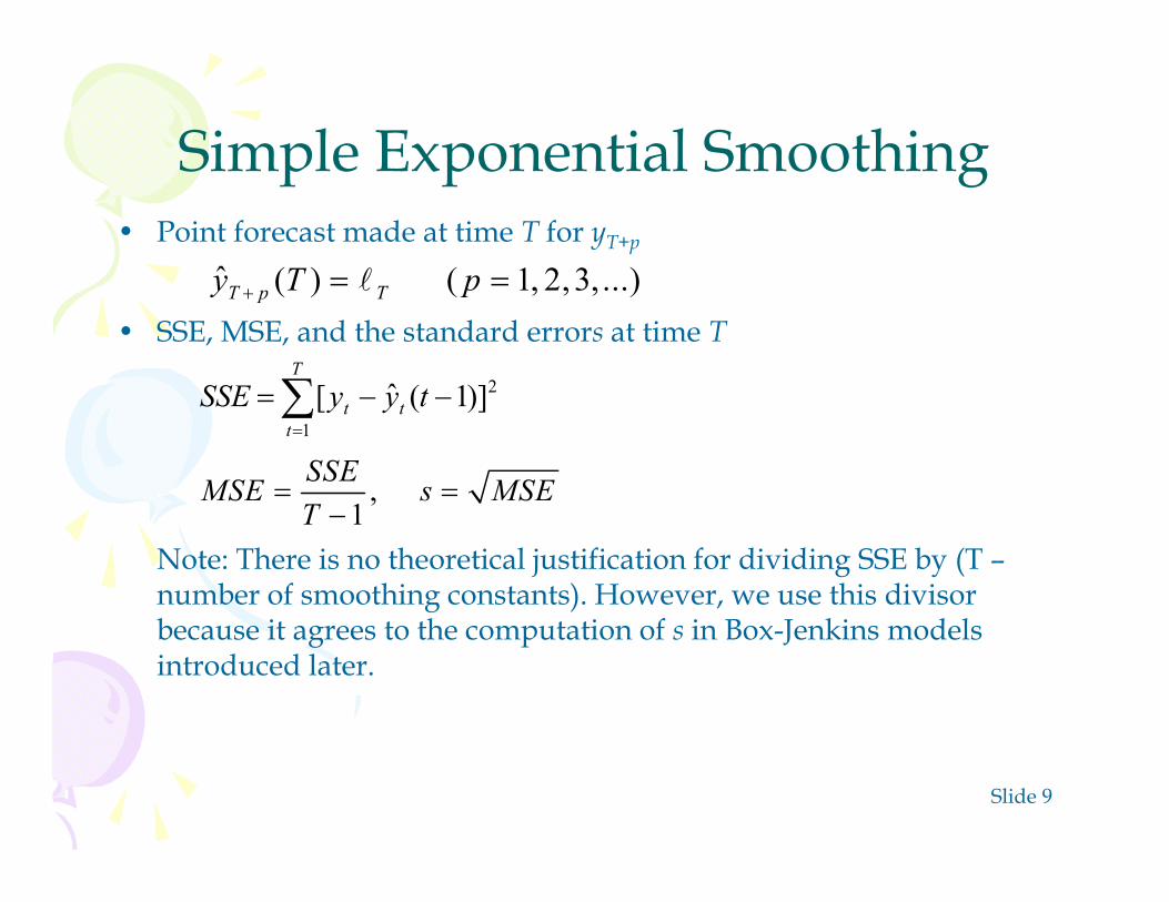
Simple Exponential Smoothing• Point forecast made at time T for yT+p
• SSE, MSE, and the standard errors at time T
Note: There is no theoretical justification for dividing SSE by (T –number of smoothing constants). However, we use this divisor because it agrees to the computation of s in Box-Jenkins models introduced later.
,1
SSEMSE s MSET
ˆ ( ) ( 1, 2,3, ...)T p Ty T p
T
ttt tyySSE
1
2)]1(ˆ[

Slide 10
Example: Cod Catch• The Bay City Seafood Company recorded the monthly cod
catch for the previous two years, as given below. Cod Catch (In Tons)
Month Year 1 Year 2
January 362 276
February 381 334
March 317 394
April 297 334
May 399 384
June 402 314
July 375 344
August 349 337
September 386 345
October 328 362
November 389 314
December 343 365
Slide 11
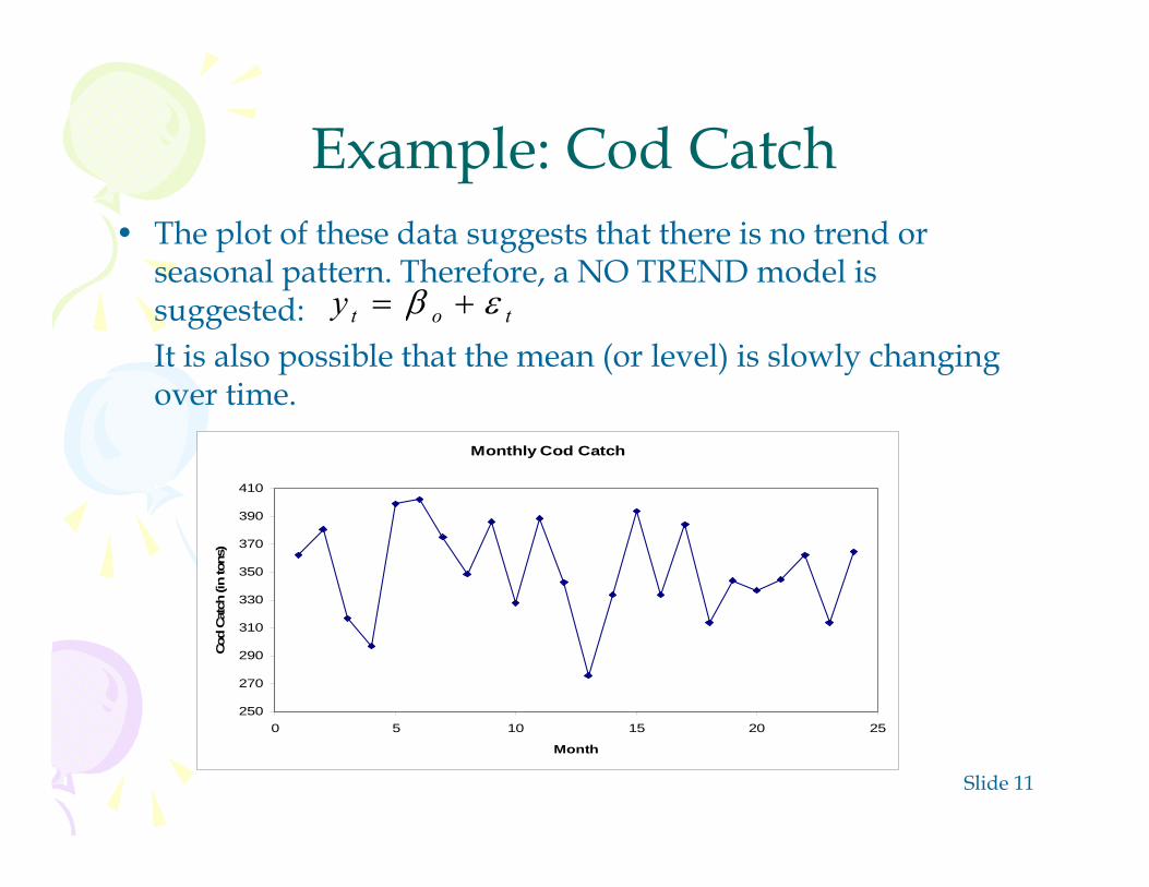
Example: Cod Catch• The plot of these data suggests that there is no trend or
seasonal pattern. Therefore, a NO TREND model is suggested: It is also possible that the mean (or level) is slowly changing over time.
toty
Monthly Cod Catch
250
270
290
310
330
350
370
390
410
0 5 10 15 20 25
Month
Cod
Catc
h (in
tons
)

Slide 12
Example: Cod Catch• Step 1: Compute ℓ0 by averaging the first twelve time
series values.
Though there is no theoretical justification, it is a common practice to calculate initial estimates of exponential smoothing procedures by using HALF of the historical data.
12
10
362 381 ... 343 360.666712 12
tt
y
Slide 13
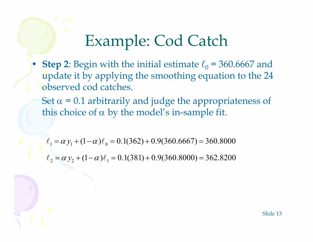
Example: Cod Catch• Step 2: Begin with the initial estimate ℓ0 = 360.6667 and
update it by applying the smoothing equation to the 24 observed cod catches. Set = 0.1 arbitrarily and judge the appropriateness of this choice of by the model’s in-sample fit.
1 1 0(1 ) 0.1(362) 0.9(360.6667) 360.8000y
2 2 1(1 ) 0.1(381) 0.9(360.8000) 362.8200y

Slide 14
One-period-ahead Forecastingn alpha SSE MSE s24 0.1 28735.1092 1249.3526 35.3462
Time Smoothed Estimate Forecast Made Forecast Squared ForecastPeriod y for Level Last Period Error Error
0 360.66671 362 360.8000 360.6667 1.3333 1.77772 381 362.8200 360.8000 20.2000 408.03883 317 358.2380 362.8200 -45.8200 2099.47494 297 352.1142 358.2380 -61.2380 3750.09565 399 356.8028 352.1142 46.8858 2198.27626 402 361.3225 356.8028 45.1972 2042.78697 375 362.6903 361.3225 13.6775 187.07358 349 361.3212 362.6903 -13.6903 187.42349 386 363.7891 361.3212 24.6788 609.041110 328 360.2102 363.7891 -35.7891 1280.860911 389 363.0892 360.2102 28.7898 828.852312 343 361.0803 363.0892 -20.0892 403.575313 276 352.5722 361.0803 -85.0803 7238.651714 334 350.7150 352.5722 -18.5722 344.928115 394 355.0435 350.7150 43.2850 1873.589916 334 352.9392 355.0435 -21.0435 442.829517 384 356.0452 352.9392 31.0608 964.775618 314 351.8407 356.0452 -42.0452 1767.802719 344 351.0566 351.8407 -7.8407 61.476920 337 349.6510 351.0566 -14.0566 197.589421 345 349.1859 349.6510 -4.6510 21.631722 362 350.4673 349.1859 12.8141 164.201523 314 346.8206 350.4673 -36.4673 1329.863824 365 348.6385 346.8206 18.1794 330.4918

Slide 15
Example: Cod Catch• Results associated with different values of
Smoothing Constant
Sum of Squared Errors
0.1 28735.11
0.2 30771.73
0.3 33155.54
0.4 35687.69
0.5 38364.24
0.6 41224.69
0.7 44324.09
0.8 47734.09

Slide 16
Example: Cod Catch• Step 3: Find a good value of that provides the
minimum value for MSE (or SSE).– Use Solver in Excel as an illustration
SSE
alpha

Slide 17
Example: Cod Catch

Slide 18
Holt’s Trend Corrected Exponential Smoothing
• If a time series is increasing or decreasing approximately at a fixed rate, then it may be described by the LINEAR TREND model
If the values of the parameters β0 and β1 are slowly changing over time, Holt’s trend corrected exponential smoothing method can be applied to the time series observations.
Note: When neither β0 nor β1 is changing over time, regression can be used to forecast future values of yt.
• Level (or mean) at time T: β0 + β1TGrowth rate (or trend): β1
tt ty 10
Slide 19
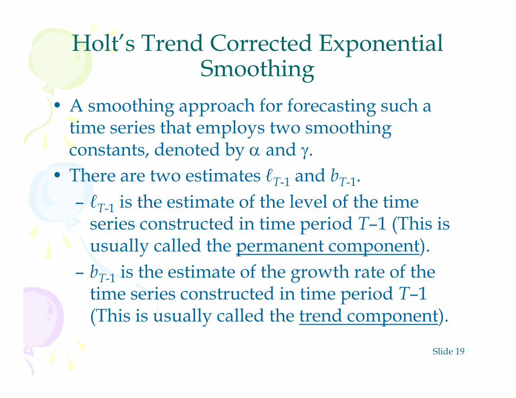
Holt’s Trend Corrected Exponential Smoothing
• A smoothing approach for forecasting such a time series that employs two smoothing constants, denoted by and .
• There are two estimates ℓT-1 and bT-1.– ℓT-1 is the estimate of the level of the time
series constructed in time period T–1 (This is usually called the permanent component).
– bT-1 is the estimate of the growth rate of the time series constructed in time period T–1 (This is usually called the trend component).
Slide 20
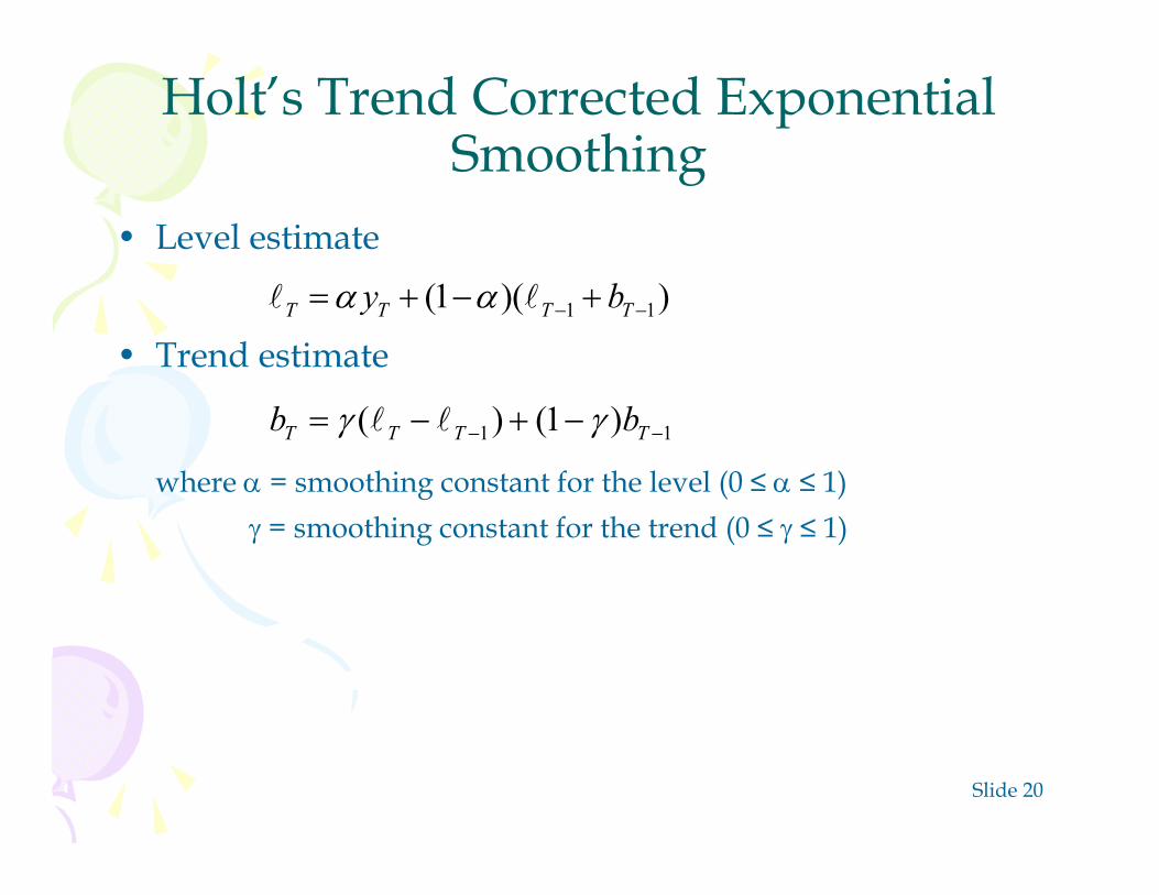
Holt’s Trend Corrected Exponential Smoothing
• Level estimate
• Trend estimate
where = smoothing constant for the level (0 ≤ ≤ 1) = smoothing constant for the trend (0 ≤ ≤ 1)
1 1(1 )( )T T T Ty b
1 1( ) (1 )T T T Tb b

Slide 21
Holt’s Trend Corrected Exponential Smoothing
• Point forecast made at time T for yT+p
• MSE and the standard error s at time T
,2
SSEMSE s MSET
ˆ ( ) ( 1, 2,3,...)T p T Ty T pb p
T
ttt tyySSE
1
2)]1(ˆ[
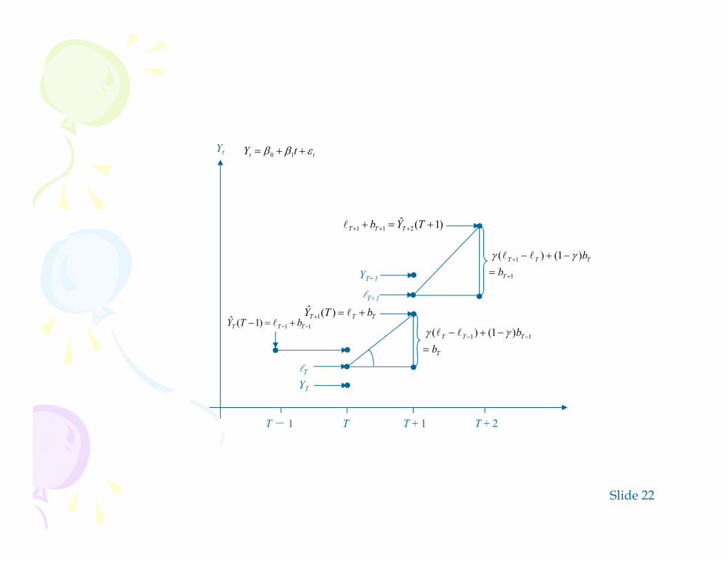
Slide 22
T - 1 T + 1 T + 2T
Yt
YT
T
YT+1
T+1
TTT bTY )(ˆ1
)1(ˆ211 TYb TTT
tt tY 10
11)1(ˆ TTT bTY
1
1 )1()(
T
TTT
bb
T
TTT
bb
11 )1()(

Slide 23
Procedures of Holt’s Trend Corrected Exponential Smoothing
• Use the example of Thermostat Sales as an illustration
150
200
250
300
350
0 10 20 30 40 50 60
Time
Ther
mos
tat S
ales
(y)
Slide 24
Procedures of Holt’s Trend Corrected Exponential Smoothing
• Findings: – Overall an upward trend– The growth rate has been changing over the
52-week period– There is no seasonal pattern Holt’s trend corrected exponential
smoothing method can be applied

Slide 25
Procedures of Holt’s Trend Corrected Exponential Smoothing
• Step 1: Obtain initial estimates ℓ0 and b0 by fitting a least squares trend line to HALF of the historical data. – y-intercept = ℓ0; slope = b0

Slide 26
Procedures of Holt’s Trend Corrected Exponential Smoothing
• Example – Fit a least squares trend line to the first 26
observations– Trend line
– ℓ0 = 202.6246; b0 = – 0.3682
ˆ 202.6246 0.3682ty t

Slide 27
Procedures of Holt’s Trend Corrected Exponential Smoothing
• Step 2: Calculate a point forecast of y1 from time 0
• Example
1 0 0ˆ (0) 202.6246 0.3682 202.2564y b
ˆ ( ) 0, 1T p T Ty T pb T p
Slide 28
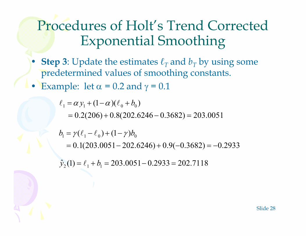
Procedures of Holt’s Trend Corrected Exponential Smoothing
• Step 3: Update the estimates ℓT and bT by using some predetermined values of smoothing constants.
• Example: let = 0.2 and = 0.1
1 1 0 0(1 )( )0.2(206) 0.8(202.6246 0.3682) 203.0051
y b
1 1 0 0( ) (1 )0.1(203.0051 202.6246) 0.9( 0.3682) 0.2933
b b
2 1 1ˆ (1) 203.0051 0.2933 202.7118y b

Slide 29
…… ……

Slide 30
Procedures of Holt’s Trend Corrected Exponential Smoothing
• Step 4: Find the best combination of and that minimizes SSE (or MSE)
• Example: Use Solver in Excel as an illustrationSSE
alpha
gamma

Slide 31
…… ……

Slide 32
Holt’s Trend Corrected Exponential Smoothing
• p-step-ahead forecast made at time T
• Example- In period 52, the one-period-ahead sales forecast for
period 53 is
– In period 52, the three-period-ahead sales forecast for period 55 is
ˆ ( ) ( 1, 2,3,...)T p T Ty T pb p
53 52 52ˆ (52) 315.9460 4.5040 320.45y b
55 52 52ˆ (52) 3 315.9460 3(4.5040) 329.458y b

Slide 33
Holt’s Trend Corrected Exponential Smoothing
• Example – If we observe y53 = 330, we can either find a new set
of (optimal) and that minimize the SSE for 53 periods, or
– we can simply revise the estimate for the level and growth rate and recalculate the forecasts as follows:
53 53 52 52(1 )( )0.247(330) 0.753(315.946 4.5040) 322.8089
y b
53 53 52 52( ) (1 )0.095(322.8089 315.9460) 0.905(4.5040) 4.7281
b b
54 53 53ˆ (53) 322.8089 4.7281 327.537y b
55 53 53ˆ (53) 2 322.8089 2(4.7281) 332.2651y b
Slide 34
Holt-Winters Methods• Two Holt-Winters methods are designed for time series
that exhibit linear trend - Additive Holt-Winters method: used for time series
with constant (additive) seasonal variations– Multiplicative Holt-Winters method: used for time
series with increasing (multiplicative) seasonal variations
• Holt-Winters method is an exponential smoothing approach for handling SEASONAL data.
• The multiplicative Holt-Winters method is the better known of the two methods.
Slide 35
Multiplicative Holt-Winters Method• It is generally considered to be best suited to forecasting
time series that can be described by the equation:
– SNt: seasonal pattern– IRt: irregular component
• This method is appropriate when a time series has a linear trend with a multiplicative seasonal pattern for which the level (β0+ β1t), growth rate (β1), and the seasonal pattern (SNt) may be slowly changing over time.
0 1( )t t ty t SN IR

Slide 36
Multiplicative Holt-Winters Method• Estimate of the level
• Estimate of the growth rate (or trend)
• Estimate of the seasonal factor
where , , and δ are smoothing constants between 0 and 1, L = number of seasons in a year (L = 12 for monthly data,
and L = 4 for quarterly data)
1 1( / ) (1 )( )T T T L T Ty sn b
1 1( ) (1 )T T T Tb b
( / ) (1 )T T T T Lsn y sn

Slide 37
Multiplicative Holt-Winters Method• Point forecast made at time T for yT+p
• MSE and the standard errors at time T
ˆ ( ) ( ) ( 1, 2,3,...)T p T T T p Ly T pb sn p
,3
SSEMSE s MSET
T
ttt tyySSE
1
2)]1(ˆ[
Slide 38
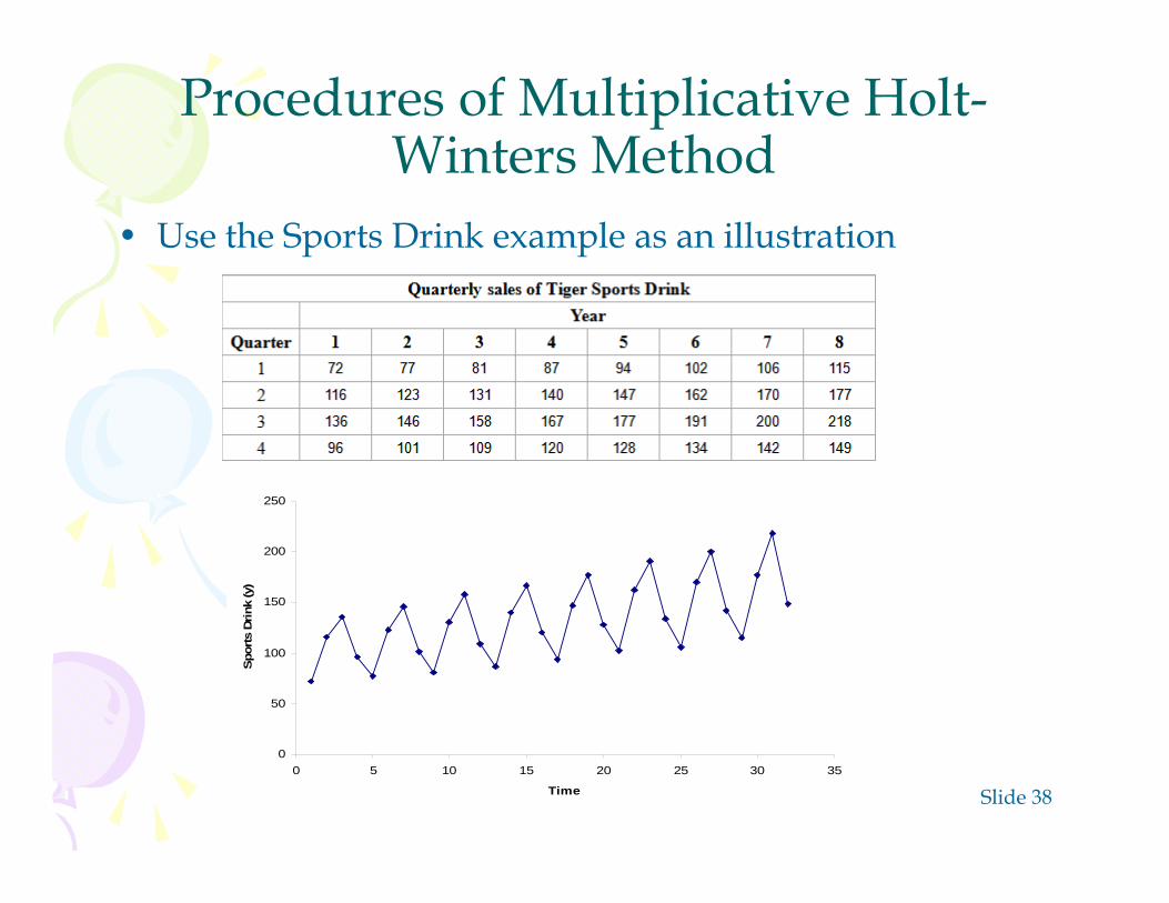
Procedures of Multiplicative Holt-Winters Method
• Use the Sports Drink example as an illustration
0
50
100
150
200
250
0 5 10 15 20 25 30 35
Time
Spo
rts D
rink
(y)

Slide 39
Procedures of Multiplicative Holt-Winters Method
• Observations: – Linear upward trend over the 8-year period– Magnitude of the seasonal span increases as
the level of the time series increases Multiplicative Holt-Winters method can be
applied to forecast future sales

Slide 40
Procedures of Multiplicative Holt-Winters Method
• Step 1: Obtain initial values for the level ℓ0, the growth rate b0, and the seasonal factors sn-3, sn-2, sn-1, and sn0, by fitting a least squares trend line to at least four or five years of the historical data. – y-intercept = ℓ0; slope = b0

Slide 41
Procedures of Multiplicative Holt-Winters Method
• Example – Fit a least squares trend line to the first 16
observations– Trend line
– ℓ0 = 95.2500; b0 = 2.4706
ˆ 95.2500 2.4706ty t

Slide 42
Procedures of Multiplicative Holt-Winters Method
• Step 2: Find the initial seasonal factors1. Compute for the in-sample observations used
for fitting the regression. In this example, t = 1, 2, …, 16.
ˆty
1
2
16
ˆ 95.2500 2.4706(1) 97.7206ˆ 95.2500 2.4706(2) 100.1912......ˆ 95.2500 2.4706(16) 134.7794
yy
y

Slide 43
Procedures of Multiplicative Holt-Winters Method
• Step 2: Find the initial seasonal factors2. Detrend the data by computing for each
time period that is used in finding the least squares regression equation. In this example, t = 1, 2, …, 16.
ˆ/t t tS y y
1 1 1
2 2 2
16 16 16
ˆ/ 72 / 97.7206 0.7368ˆ/ 116 /100.1912 1.1578
......ˆ/ 120 /134.7794 0.8903
S y yS y y
S y y

Slide 44
Procedures of Multiplicative Holt-Winters Method
• Step 2: Find the initial seasonal factors3. Compute the average seasonal values for each of the L seasons. The L averages are found by computing the average of the detrended values for the corresponding season. For example, for quarter 1,
1 5 9 13[1] 4
0.7368 0.7156 0.6894 0.6831 0.70624
S S S SS

Slide 45
Procedures of Multiplicative Holt-Winters Method
• Step 2: Find the initial seasonal factors4. Multiply the average seasonal values by the
normalizing constant
such that the average of the seasonal factors is 1. The initial seasonal factors are
[ ]1
L
ii
LCFS
[ ] ( ) ( 1, 2, ..., )i L isn S CF i L

Slide 46
Procedures of Multiplicative Holt-Winters Method
• Step 2: Find the initial seasonal factors4. Multiply the average seasonal values by the
normalizing constant such that the average of the seasonal factors is 1. • Example
CF = 4/3.9999 = 1.0000
3 1 4 [1]
2 2 4 [2]
1 3 4 [3]
0 4 4 [1]
( ) 0.7062(1) 0.7062
( ) 1.1114(1) 1.1114
( ) 1.2937(1) 1.2937
( ) 0.8886(1) 0.8886
sn sn S CF
sn sn S CF
sn sn S CF
sn sn S CF

Slide 47
Procedures of Multiplicative Holt-Winters Method
• Step 3: Calculate a point forecast of y1 from time 0 using the initial values
1 0 0 1 4 0 0 3
ˆ ( ) ( ) ( 0, 1)ˆ (0) ( ) ( )
(95.2500 2.4706)(0.7062)69.0103
T p T T T p Ly T pb sn T p
y b sn b sn

Slide 48
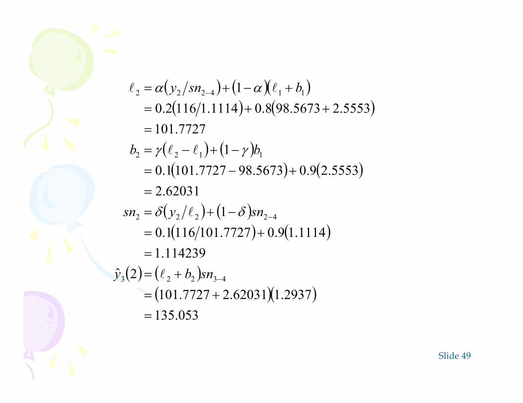
Procedures of Multiplicative Holt-Winters Method
• Step 4: Update the estimates ℓT, bT, and snT by using some predetermined values of smoothing constants.
• Example: let = 0.2, = 0.1, and δ = 0.1
1 1 1 4 0 0( / ) (1 )( )0.2(72 / 0.7062) 0.8(95.2500 2.4706) 98.5673
y sn b
1 1 0 0( ) (1 )0.1(98.5673 95.2500) 0.9(2.4706) 2.5553
b b
2 1 1 2 4ˆ (1) ( )(98.5673 2.5553)(1.1114) 112.3876
y b sn
1 1 1 1 4( / ) (1 )0.1(72 / 98.5673) 0.9(0.7062) 0.7086
sn y sn
Slide 49
053.1352937.162031.27727.101
2ˆ114239.1
1114.19.07727.1011161.01
62031.25553.29.05673.987727.1011.0
17727.101
5553.25673.988.01114.11162.01
43223
42222
1122
114222
snby
snysn
bb
bsny

Slide 50
945.777086.065212.23464.107
4ˆ889170.0
8886.09.03464.107961.01
65212.26349.29.05393.1043464.1071.0
13464.107
6349.25393.1048.08886.0962.01
45445
44444
3344
334444
snby
snysn
bb
bsny

Slide 51
…… ……

Slide 52
Procedures of Multiplicative Holt-Winters Method
• Step 5: Find the most suitable combination of , , and δ that minimizes SSE (or MSE)
• Example: Use Solver in Excel as an illustrationSSE
alpha
gamma
delta

Slide 53
…… ……

Slide 54
Multiplicative Holt-Winters Method• p-step-ahead forecast made at time T
• Example
ˆ ( ) ( ) ( 1,2,3,...)T p T T T p Ly T pb sn p
33 32 32 33 4ˆ (32) ( ) (168.1213 2.3028)(0.7044) 120.0467y b sn
34 32 32 34 4ˆ (32) ( 2 ) [168.1213 2(2.3028)](1.1038) 190.6560y b sn
35 32 32 35 4ˆ (32) ( 3 ) [(168.1213 3(2.3028)](1.2934) 226.3834y b sn
36 32 32 36 4ˆ (32) ( 4 ) [(168.1213 4(2.3028)](0.8908) 157.9678y b sn

Slide 55
Multiplicative Holt-Winters Method• Example
Forecast Plot for Sports Drink Sales
0
50
100
150
200
250
0 5 10 15 20 25 30 35 40
Time
Fore
cast
s
Observed valuesForecasts

Slide 56
Additive Holt-Winters Method• It is generally considered to be best suited to forecasting
a time series that can be described by the equation:
– SNt: seasonal pattern– IRt: irregular component
• This method is appropriate when a time series has a linear trend with a constant (additive) seasonal pattern such that the level (β0+ β1t), growth rate (β1), and the seasonal pattern (SNt) may be slowly changing over time.
ttt IRSNty )( 10

Slide 57
Additive Holt-Winters Method• Estimate of the level
• Estimate of the growth rate (or trend)
• Estimate of the seasonal factor
where , , and δ are smoothing constants between 0 and 1, L = number of seasons in a year (L = 12 for monthly data,
and L = 4 for quarterly data)
))(1()( 11 TTLTTT bsny
11 )1()( TTTT bb
LTTTT snysn )1()(
Slide 58
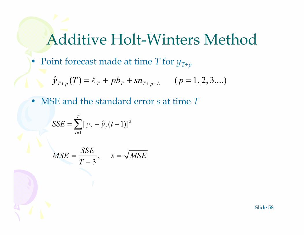
Additive Holt-Winters Method• Point forecast made at time T for yT+p
• MSE and the standard error s at time T
,3
SSEMSE s MSET
3,...) 2, 1,( )(ˆ psnpbTy LpTTTpT
T
ttt tyySSE
1
2)]1(ˆ[

Slide 59
Procedures of Additive Holt-Winters Method
• Consider the Mountain Bike example,
0
10
20
30
40
50
60
0 2 4 6 8 10 12 14 16 18
Time
Bike
sal
es (y
)
Slide 60
Procedures of Additive Holt-Winters Method
• Observations: – Linear upward trend over the 4-year period– Magnitude of seasonal span is almost constant
as the level of the time series increases Additive Holt-Winters method can be
applied to forecast future sales

Slide 61
Procedures of Additive Holt-Winters Method
• Step 1: Obtain initial values for the level ℓ0, the growth rate b0, and the seasonal factors sn-3, sn-2, sn-1, and sn0, by fitting a least squares trend line to at least four or five years of the historical data. – y-intercept = ℓ0; slope = b0

Slide 62
Procedures of Additive Holt-Winters Method
• Example – Fit a least squares trend line to all 16 observations– Trend line
– ℓ0 = 20.85; b0 = 0.9809
tyt 980882.085.20ˆ

Slide 63
Procedures of Additive Holt-Winters Method
• Step 2: Find the initial seasonal factors1. Compute for each time period that is used in
finding the least squares regression equation. In this example, t = 1, 2, …, 16.
ˆty
1
2
16
ˆ 20.85 0.980882(1) 21.8309ˆ 20.85 0.980882(2) 22.8118......ˆ 20.85 0.980882(16) 36.5441
yy
y

Slide 64
Procedures of Additive Holt-Winters Method
• Step 2: Find the initial seasonal factors2. Detrend the data by computing for each
observation used in the least squares fit. In this example, t = 1, 2, …, 16.
ttt yyS ˆ
5441.115441.3625ˆ......
1882.88112.2231ˆ8309.118309.2110ˆ
161616
222
111
yyS
yySyyS

Slide 65
Procedures of Additive Holt-Winters Method
• Step 2: Find the initial seasonal factors3. Compute the average seasonal values for each of the L seasons. The L averages are found by computing the average of the detrended values for the corresponding season. For example, for quarter 1,
2162.144
)6015.14()6779.15()7544.14()8309.11(
413951
]1[
SSSSS

Slide 66
Procedures of Additive Holt-Winters Method
• Step 2: Find the initial seasonal factors4. Compute the average of the L seasonal factors. The
average should be 0.

Slide 67
Procedures of Additive Holt-Winters Method
• Step 3: Calculate a point forecast of y1 from time 0 using the initial values
7.6147(-14.2162)0.980920.85 )0(ˆ
1),0( )(ˆ
30041001
snbsnby
pTsnpbTy LpTTTpT
Slide 68
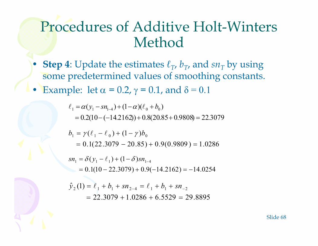
Procedures of Additive Holt-Winters Method
• Step 4: Update the estimates ℓT, bT, and snT by using some predetermined values of smoothing constants.
• Example: let = 0.2, = 0.1, and δ = 0.1
3079.22)9808.085.20(8.0))2162.14(10(2.0 ))(1()( 004111
bsny
0286.1)9809.0(9.0)85.203079.22(1.0 )1()( 0011
bb
0254.14)2162.14(9.0)3079.2210(1.0 )1()( 41111
snysn
8895.295529.60286.13079.22 )1(ˆ 21142112
snbsnby

Slide 69

Slide 70
Procedures of Additive Holt-Winters Method
• Step 5: Find the most suitable combination of , , and δ that minimizes SSE (or MSE)
• Example: Use Solver in Excel as an illustrationSSE
alpha
gamma
delta

Slide 71

Slide 72
Additive Holt-Winters Method• p-step-ahead forecast made at time T
• Example
3,...) 2, 1,( )(ˆ psnpbTy LpTTTpT
1073.232162.149809.03426.36)16(ˆ 417161617 snby
8573.445529.6)9809.0(23426.362)16(ˆ 418161618 snby
8573.575721.18)9809.0(33426.363)16(ˆ 419161619 snby
3573.299088.10)9809.0(43426.364)16(ˆ 420161620 snby

Slide 73
Additive Holt-Winters Method• Example
Forecast Plot for Mountain Bike Sales
0
10
20
30
40
50
60
70
0 2 4 6 8 10 12 14 16 18 20
Time
Fore
cast
s
Observed valuesForecasts
Slide 74
Chapter Summary• Simple Exponential Smoothing
– No trend, no seasonal pattern• Holt’s Trend Corrected Exponential Smoothing
– Trend, no seasonal pattern• Holt-Winters Methods
– Both trend and seasonal pattern• Multiplicative Holt-Winters method• Additive Holt-Winters Method