exponentiated gradient algorithms for conditional random fields and max...
TRANSCRIPT

Journal of Machine Learning Research ? (2007) ??–?? Submitted ??/07; Published ??/07
1
Exponentiated Gradient Algorithms for Conditional RandomFields and Max-Margin Markov Networks
Michael Collins∗ [email protected]
Amir Globerson∗ [email protected]
Terry Koo∗ [email protected]
Xavier Carreras [email protected]
Computer Science and Artificial Intelligence LaboratoryMassachusetts Institute of TechnologyCambridge, MA 02139, USAPeter L. Bartlett [email protected]
University of California, BerkeleyDivision of Computer Science and Department of StatisticsBerkeley, CA 94720, USA
Editor: ...
Abstract
Log-linear and maximum-margin models are two commonly-used methods in supervisedmachine learning, and are frequently used in structured prediction problems. Efficientlearning of parameters in these models is therefore an important problem, and becomes akey factor when learning from very large data sets. This paper describes exponentiatedgradient (EG) algorithms for training such models, where EG updates are applied to theconvex dual of either the log-linear or max-margin objective function; the dual in both thelog-linear and max-margin cases corresponds to minimizing a convex function with simplexconstraints. We study both batch and online variants of the algorithm, and provide ratesof convergence for both cases. In the max-margin case, O( 1
ε ) EG updates are requiredto reach a given accuracy ε in the dual; in contrast, for log-linear models only O(log( 1
ε ))updates are required. For both the max-margin and log-linear cases, our bounds suggestthat the online EG algorithm requires a factor of n less computation to reach a desiredaccuracy than the batch EG algorithm, where n is the number of training examples. Ourexperiments confirm that the online algorithms are much faster than the batch algorithmsin practice. We describe how the EG updates factor in a convenient way for structuredprediction problems, allowing the algorithms to be efficiently applied to problems such assequence learning or natural language parsing. We perform extensive evaluation of thealgorithms, comparing them to to L-BFGS and stochastic gradient descent for log-linearmodels, and to SVM-Struct for max-margin models. The algorithms are applied to multi-class problems as well as a more complex large-scale parsing task. In all these settings, theEG algorithms presented here outperform the other methods.
Keywords: Exponentiated Gradient, Log-Linear Models, Maximum-Margin Models,Structured Prediction, Conditional Random Fields
∗. These authors contributed equally.
c©2007 Michael Collins, Amir Globerson, Terry Koo, Xavier Carreras, Peter L. Bartlett.
Collins, Globerson, Koo, Carreras and Bartlett
1. Introduction
Structured prediction problems involve learning to map inputs x to labels y, where thelabels have rich internal structure, and where the set of possible labels for a given input istypically exponential in size. Examples of structured prediction problems include sequencelabeling and natural language parsing. Several models that implement learning in thisscenario have been proposed over the last few years, including log-linear models such asconditional random fields (CRFs, Lafferty et al., 2001), and maximum-margin models suchas maximum-margin Markov networks (Taskar et al., 2004a).
For both log-linear and max-margin models, learning is framed as minimization of aregularized loss function which is convex. In spite of the convexity of the objective function,finding the optimal parameters for these models can be computationally intensive, especiallyfor very large data sets. This problem is exacerbated in structured prediction problems,where the large size of the set of possible labels adds an additional layer of complexity.The development of efficient optimization algorithms for learning in structured predictionproblems is therefore an important problem.
In this paper we describe learning algorithms that exploit the structure of the dualoptimization problems for log-linear and max-margin models. For both log-linear and max-margin models the dual problem corresponds to the minimization of a convex function Qsubject to simplex constraints (Jaakkola and Haussler, 1999; Lebanon and Lafferty, 2002;Taskar et al., 2004a). More specifically, the goal is to find
argmin∀i, αi∈∆
Q(α1,α2, . . . ,αn) (1)
where n is the number of training examples, each αi is a vector of dual variables for the i’thtraining example, and Q(α) is a convex function.1 The size of each vector αi is |Y|, whereY is the set of possible labels for any training example. Furthermore, αi is constrained tobelong to the simplex of distributions over Y, defined as:
∆ =
p ∈ R|Y| : py ≥ 0 ,∑y∈Y
py = 1
(2)
Thus each αi is constrained to form a distribution over the set of possible labels. Themax-margin and log-linear problems differ only in their definition of Q.
The algorithms in this paper make use of exponentiated gradient (EG) updates (Kivinenand Warmuth, 1997) in solving the problem in Eq. 1, in particular for the cases of log-linear or max-margin models. We focus on two classes of algorithms, which we call batchand online. In the batch case, the entire set of αi variables is updated simultaneously ateach iteration of the algorithm; in the online case, a single αi variable is updated at eachstep. The “online” case essentially corresponds to coordinate-descent on the dual functionQ, and is similar to the SMO algorithm (Platt, 1998) for training SVMs. The onlinealgorithm has the advantage of updating the parameters after every sample point, ratherthan after making a full pass over the training examples; intuitively, this should lead toconsiderably faster rates of convergence when compared to the batch algorithm, and indeed
1. In what follows we use α to denote the variables α1, . . . ,αn.
2

Exponentiated Gradient Algorithms for CRFs and Max-Margin Markov Networks
our experimental and theoretical results support this intuition. A different class of onlinealgorithms consists of stochastic gradient descent (SGD) and its variants (e.g., see LeCunet al., 1998; Vishwanathan et al., 2006). In contrast to SGD, however, the EG algorithm isguaranteed to improve the dual objective at each step, and this objective may be calculatedafter each example without performing a pass over the entire data set. This is particularlyconvenient when making a choice of learning rate in the updates.
We describe theoretical results concerning the convergence of the EG algorithms, as wellas experiments. Our key results are as follows:
• For the max-margin case, we show that O(1ε ) time is required for both the online
and batch algorithms to converge to within ε of the optimal value of Q(α). Thisis qualitatively similar to recent results in the literature for max-margin approaches(e.g., see Shalev-Shwartz et al., 2007). For log-linear models, we show convergencerates of O(log(1
ε )), a significant improvement over the max-margin case.
• For both the max-margin and log-linear cases, our bounds suggest that the onlinealgorithm requires a factor of n less computation to reach a desired accuracy, where n isthe number of training examples. Our experiments confirm that the online algorithmsare much faster than the batch algorithms in practice.
• We describe how the EG algorithms can be efficiently applied to an important classof structured prediction problems where the set of labels Y is exponential in size. Inthis case the number of dual variables is also exponential in size, making algorithmswhich deal directly with the αi variables intractable. Following Bartlett et al. (2005),we focus on a formulation where each label y is represented as a set of “parts”, forexample corresponding to labeled cliques in a max-margin network, or context-freerules in a parse tree. Under an assumption that part-based marginals can be calculatedefficiently—for example using junction tree algorithms for CRFs, or the inside-outsidealgorithm for context-free parsing—the EG algorithms can be implemented efficientlyfor both max-margin and log-linear models.
• In our experiments we compare the online EG algorithm to various state of the artalgorithms. For log-linear models, we compare to the L-BFGS algorithm (Byrd et al.,1995) and to stochastic gradient descent. For max-margin models we compare to theSVM-Struct algorithm of Tsochantaridis et al. (2004). The methods are applied toa standard multi-class learning problem, as well as a more complex natural languageparsing problem. In both settings we show that the EG algorithm converges to theoptimum much faster than these algorithms.
• In addition to proving convergence results for the definition of Q(α) used in max-margin and log-linear models, we give theorems which may be useful when optimizingother definitions of Q(α) using EG updates. In particular, we give conditions forconvergence which depend on bounds relating the Bregman divergence derived fromQ(α) to the Kullback-Liebler divergence. Depending on the form of these bounds fora particular Q(α), either O(1
ε ) or O(log(1ε )) rates of convergence can be derived.
The rest of this paper is organized as follows. In Section 2, we introduce the log-linear and max-margin learning problems, and describe their dual optimization problems.
3

Collins, Globerson, Koo, Carreras and Bartlett
Section 3 describes the batch and online EG algorithms; in Section 4, we describe howthe algorithms can be efficiently applied to structured prediction problems. Section 5 thengives convergence proofs for the batch and online cases. Section 6 discusses related work.Sections 7 and 8 give experiments, and Section 9 discusses our results.
This work builds on previous work described by Bartlett et al. (2005) and Globersonet al. (2007). Bartlett et al. (2005) described the application of the EG algorithm to max-margin parameter estimation, and showed how the method can be applied efficiently to part-based formulations. Globerson et al. (2007) extended the approach to log-linear parameterestimation, and gave new convergence proofs for both max-margin and log-linear estimation.The work in the current paper gives several new results. We prove rates of convergence fora randomized version of the EG online algorithm; previous work on EG algorithms hadnot given convergence rates for the online case. We also report new experiments, includingexperiments with the randomized strategy. Finally, the O(log(1
ε )) convergence rates for thelog-linear case are new. The results in Globerson et al. (2007) gave O(1
ε ) rates for the batchalgorithm for log-linear models, and did not give any theoretical rates of convergence forthe online case.
2. Primal and Dual Problems for Regularized Loss Minimization
2.1 The Primal Problems
Consider a supervised learning setting with objects x ∈ X and labels y ∈ Y.2 In thestructured learning setting, the labels may be sequences, trees, or other high-dimensionaldata with internal structure. Assume we are given a function φ(x, y) : X × Y → Rd thatmaps (x, y) pairs to feature vectors. Our goal is to construct a linear prediction rule
f(x,w) = arg maxy∈Y
w · φ(x, y) (3)
with parameters w ∈ Rd, such that f(x,w) is a good approximation of the true label of x.The parameters w are learned by minimizing a regularized loss
L(w; {(xi, yi)}ni=1, C) =n∑i=1
`(w, xi, yi) +C
2‖w‖2 (4)
defined over a labeled training set {(xi, yi)}ni=1. Here C > 0 is a constant determining theamount of regularization. The function ` measures the loss incurred in using w to predictthe label of xi, given that the true label is yi.
In this paper we will consider two definitions for `(w, xi, yi). The first definition, orig-inally introduced by Taskar et al. (2004a), is a variant of the hinge loss, and is defined asfollows:
`MM(w, xi, yi) = maxy∈Y
[e(xi, yi, y)−w · (φ(xi, yi)− φ(xi, y))
]. (5)
Here e(xi, yi, y) is some measure of the error incurred in predicting y instead of yi as thelabel of xi. We assume that e(xi, yi, yi) = 0 for all i, so that no loss is incurred for
2. In general the set of labels for a given example x may be a set Y(x) that depends on x; in fact, in ourexperiments on dependency parsing Y does depend on x. For simplicity, in this paper we use the fixednotation Y for all x; it is straightforward to extend our notation to the more general case.
4

Exponentiated Gradient Algorithms for CRFs and Max-Margin Markov Networks
correct prediction, and therefore `MM(w, xi, yi) is always non-negative. This loss functioncorresponds to a maximum-margin approach, which explicitly penalizes training examplesfor which, for some y 6= yi,
w · (φ(xi, yi)− φ(xi, y)) < e(xi, yi, y).
The second loss function that we will consider is based on log-linear models, and iscommonly used in conditional random fields (CRFs, Lafferty et al., 2001). First define theconditional distribution
p(y |x; w) =1Zxew·φ(x,y), (6)
where Zx =∑
y ew·φ(x,y) is the partition function. The loss function is then the negative
log-likelihood under the parameters w:
`LL(w, xi, yi) = − log p(yi |xi; w) . (7)
The function L is convex in w for both definitions `MM and `LL. Furthermore, in bothcases minimization of L can be re-cast as optimization of a dual convex problem. The dualproblems in the two cases have a similar structure, as we describe in the next two sections.
2.2 The Log-Linear Dual
The problem of minimizing L with the loss function `LL can be written as
P-LL : w∗ = argminw
−∑i
log p(yi |xi; w) +C
2‖w‖2
This is a convex optimization problem, and has an equivalent convex dual which was derivedby Lebanon and Lafferty (2002). Denote the dual variables by αi,y where i = 1, . . . , n andy ∈ Y. We also use α to denote the set of all variables, and αi the set of all variablescorresponding to a given i. Thus α = [α1, . . . ,αn]. We assume α is a column vector.Define the function QLL(α) as
QLL(α) =∑i
∑y
αi,y logαi,y +1
2C‖w(α)‖2
wherew(α) =
∑i
∑y
αi,yψi,y (8)
and where ψi,y = φ(xi, yi)−φ(xi, y). We shall find the following matrix notation convenient:
QLL(α) =∑i
∑y
αi,y logαi,y +12αTAα (9)
where A is a matrix of size n|Y|×n|Y| indexed by pairs (i, y), and A(i,y),(j,z) = 1Cψi,y ·ψj,z.
5

Collins, Globerson, Koo, Carreras and Bartlett
In what follows we denote the set of distributions over Y, i.e. the |Y|-dimensionalprobability simplex, by ∆, as in Eq. 2. The Cartesian product of n distributions over Ywill be denoted by ∆n. The dual optimization problem is then
D-LL : α∗ = argmin QLL(α)s.t. α ∈ ∆n (10)
The minimum of D-LL is equal to −1 times the minimum of P-LL. The duality betweenP-LL and D-LL implies that the primal and dual solutions satisfy Cw∗ = w(α∗).
2.3 The Max-Margin Dual
When the loss is defined using `MM(w, xi, yi), the primal optimization problem is as follows:
P-MM : w∗ = argminw
−∑i
maxy
[e(xi, yi, y)−w · (φ(xi, yi)− φ(xi, y))
]+C
2‖w‖2
The dual of this minimization problem was derived in Taskar et al. (2004a) (see also Bartlettet al., 2005). We first define the dual objective
QMM(α) = −bTα+12αTAα. (11)
Here, the matrix A is as defined above and b ∈ Rn|Y| is a vector defined as bi,y = e(xi, yi, y).The convex dual for the max-margin case is then given by
D-MM : α∗ = argmin QMM(α)s.t. α ∈ ∆n (12)
The minimum of D-MM is equal to −1 times the minimum of P-MM. (Note that for D-MMthe minimizer α∗ will not be unique since A is singular; in this case we take α∗ to be anymember of the set of minimizers of QMM(α)). The optimal primal parameters are againrelated to the optimal dual parameters, through Cw∗ = w(α∗). Here again the constraintsare that αi is a distribution over Y for all i.
It can be seen that the D-LL and D-MM problems have a similar structure, in that theyboth involve minimization of a convex function Q(α) over the set ∆n. This will allow us todescribe algorithms for both problems using a common framework.
3. Exponentiated Gradient Algorithms
In this section we describe batch and online algorithms for minimizing a convex functionQ(α) subject to the constraints α ∈ ∆n. The algorithms can be applied to both the D-LLand D-MM optimization problems that were introduced in the previous section. The algo-rithms we describe are based on exponentiated gradient (EG) updates, originally introducedby Kivinen and Warmuth (1997) in the context of online learning algorithms.3
3. Kivinen and Warmuth (1997) study a setting with an infinite stream of data, as opposed to a fixed dataset which we study here. They are thus not interested in minimizing a fixed objective, but rather studyregret type bounds. This leads to algorithms and theoretical analyses that are quite different from theones considered in the current work.
6

Exponentiated Gradient Algorithms for CRFs and Max-Margin Markov Networks
The EG updates rely on the following operation. Given a sequence of distributionsα ∈ ∆n, a new sequence of distributions α′ can be obtained as
α′i,y =1Ziαi,ye
−η∇i,y ,
where ∇i,y = ∂Q(α)∂αi,y
, Zi =∑
y αi,ye−η∇i,y is a partition function ensuring normalization
of the distribution α′i, and the parameter η > 0 is a learning rate. We will also use thenotation α′i,y ∝ αi,ye−η∇i,y where the partition function should be clear from the context.
Clearly α′ ∈ ∆n by construction. For the dual function QLL(α) the gradient is
∇i,y = 1 + logαi,y +1C
w(α) ·ψi,y
and for QMM(α) the gradient is
∇i,y = −bi,y +1C
w(α) ·ψi,y
In this paper we will consider both parallel (batch), and sequential (online) applicationsof the EG updates, defined as follows:
• Batch: At every iteration the dual variables αi are simultaneously updated for alli = 1, . . . , n.
• Online: At each iteration a single example k is chosen uniformly at random from{1, . . . , n} and αk is updated to give α′k. The dual variables αi for i 6= k are leftunchanged.
Pseudo-code for the two schemes is given in Figures 1 and 2. From here on we will referto the batch and online EG algorithms applied to the log-linear dual as LLEG-Batch, andLLEG-Online respectively. Similarly, when applied to the max-margin dual, they will bereferred to as MMEG-Batch and MMEG-Online.
Note that another plausible online algorithm would be a “deterministic” algorithm thatrepeatedly cycled over the training examples in a fixed order. The motivation for thealternative, randomized, algorithm is two-fold. First, we are able to prove bounds on therate of convergence of the randomized algorithm; we have not been able to prove similarbounds for the deterministic variant. Second, our experiments show that the randomizedvariant converges significantly faster than the deterministic algorithm.
The EG online algorithm is essentially performing coordinate descent on the dual objec-tive, and is similar to SVM algorithms such as SMO (Platt, 1998). For binary classification,the exact minimum of the dual objective with respect to a given coordinate can be found inclosed form,4 and more complicated algorithms such as the exponentiated-gradient methodmay be unnecessary.5 However for multi-class or structured problems, the exact minimum
4. This is true for the max-margin case. For log-linear models, minimization with respect to a singlecoordinate is a little more involved.
5. Note, however, that it is not entirely clear that finding the exact optimum with respect to each coordinatewould result in faster convergence than the EG method.
7

Collins, Globerson, Koo, Carreras and Bartlett
Inputs: A convex function Q : ∆n → R, a learning rate η > 0.
Initialization: Set α1 to a point in the interior of ∆n.
Algorithm:
• For t = 1, . . . , T , repeat:
– For all i, y, calculate ∇i,y = ∂Q(αt)∂αi,y
– For all i, y, update αt+1i,y ∝ αti,ye−η∇i,y
Output: Final parameters αT+1.
Figure 1: A general batch EG Algorithm for minimizing Q(α) subject to α ∈ ∆n. We useαt to denote the set of parameters after t iterations.
Inputs: A convex function Q : ∆n → R, a learning rate η > 0.
Initialization: Set α1 to a point in the interior of ∆n.
Algorithm:
• For t = 1, . . . , T , repeat:
– Choose kt uniformly at random from the set {1, 2, . . . , n}
– For all y, calculate: ∇kt,y = ∂Q(αt)∂αkt,y
– For all y, update αt+1kt,y∝ αtkt,y
e−η∇kt,y .
– For all i 6= kt, set αt+1i = αti
Output: Final parameters αT+1.
Figure 2: A general randomized online EG Algorithm for minimizing Q(α) subject to α ∈∆n.
with respect to a coordinate αi (i.e., a set of |Y| dual variables) cannot be found in closedform: this is a key motivation for the use of EG algorithms in this paper.
In Section 5 we give convergence proofs for the batch and online algorithms. The tech-niques used in the convergence proofs are quite general, and could potentially be useful inderiving EG algorithms for convex functions Q other than QLL and QMM. Before giving con-vergence results for the algorithms, we describe in the next section how the EG algorithmscan be applied in structured problems.
4. Structured Prediction with the EG Algorithms
We now describe how the EG updates can be applied to structured prediction problems, forexample parameter estimation in CRFs or natural language parsing. In structured problems
8

Exponentiated Gradient Algorithms for CRFs and Max-Margin Markov Networks
the label set Y is typically very large, but labels can have useful internal structure. As oneexample, in CRFs each label y is an m-dimensional vector specifying the labeling of all mvertices in a graph. In parsing each label y is an entire parse tree. In both of these cases,the number of labels typically grows exponentially quickly with respect to the size of theinputs x.
We follow the framework for structured problems described by Bartlett et al. (2005).Each label y is defined to be a set of parts. We use R to refer to the set of all possibleparts.6 We make the assumption that the feature vector for an entire label y decomposesinto a sum over feature vectors for individual parts as follows:
φ(x, y) =∑r∈y
φ(x, r).
Note that we have overloaded φ to apply to either labels y or parts r.As one example, consider a CRF which has an underlying graph with m nodes, and a
maximum clique size of 2. Assume that each node can be labeled with one of two labels,0 or 1. In this case the labeling of an entire graph is a vector y ∈ {0, 1}m. Each possibleinput x is usually a vector in Xm for some set X , although this does not have to be thecase. Each part corresponds to a tuple (u, v, yu, yv) where (u, v) is an edge in the graph, andyu, yv are the labels for the two vertices u and v. The feature vector φ(x, r) can then trackany properties of the input x together with the labeled clique r = (u, v, yu, yv). In CRFswith clique size greater than 2, each part corresponds to a labeled clique in the graph. Innatural language parsing, each part can correspond to a context-free rule at a particularposition in the sentence x (see Bartlett et al., 2005; Taskar et al., 2004b, for more details).
The label set Y can be extremely large in structured prediction problems. For example,in a CRF with an underlying graph with m nodes and k possible labels at each node, thereare km possible labelings of the entire graph. The algorithms we have presented so farrequire direct manipulation of dual variables αi,y corresponding to each possible labelingof each training example; they will therefore be intractable in cases where there are anexponential number of possible labels. However, in this section we describe an approachthat does allow an efficient implementation of the algorithms in several cases. The approachis based on the method originally described in Bartlett et al. (2005).
The key idea is as follows. Instead of manipulating the dual variables αi for each idirectly, we will make use of alternative data structures θi for all i. Each θi is a vectorof real values θi,r for all r ∈ R. In general we will assume that there are a tractable(polynomial) number of possible parts, and therefore that the number of θi,r variables isalso polynomial. For example, for a CRF with m nodes and k labels at every node, andwhere the underlying graph has a maximum clique size of 2, each part takes the formr = (u, v, yu, yv), and there are m2k2 possible parts.
In the max-margin case, we follow Taskar et al. (2004a) and make the additional as-sumption that the error function decomposes into “local” error functions over parts:
e(xi, yi, y) =∑r∈y
e(xi, yi, r) (13)
6. As with the label set Y, the set of parts R may in general be a set R(x) that depends on x. For simplicity,we assume that R is fixed.
9

Collins, Globerson, Koo, Carreras and Bartlett
For example, when Y is a sequence of variables, the cost could be the Hamming distancebetween the correct sequence yi and the predicted sequence y; it is straightforward todecompose the Hamming distance as a sum over parts as shown above. For brevity, in whatfollows we use ei,r instead of e(xi, yi, r).
The θi variables are used to implicitly define regular dual values αi = σ(θi) whereσ : R|R| → ∆ is defined as
σy(θ) =exp
{∑r∈y θr
}∑
y′ exp{∑
r∈y′ θr
}To see how the θi variables can be updated, consider again the EG updates on the dual αvariables. The EG updates in all algorithms in this paper take the form
α′i,y =αi,y exp{−η∇i,y}∑y αi,y exp{−η∇i,y}
where for QLL
∇i,y = 1 + logαi,y +1C
w(α) · (φ(xi, yi)− φ(xi, y))
and for QMM,
∇i,y = −bi,y +1C
w(α) · (φ(xi, yi)− φ(xi, y))
where bi,y = e(xi, yi, y) as in Section 2.3.Notice that, for both objective functions, the gradients can be expressed as a sum over
parts. For the QLL objective function, this follows from the fact that αi = σ(θi) and fromthe assumption that the feature vector decomposes into parts. For the QMM objective,it follows from the latter, and the assumption that the loss decomposes into parts. Thefollowing lemma describes how EG updates on the α variables can be restated in terms ofupdates to the θ variables, provided that the gradient decomposes into parts in this way.
Lemma 1 For a given α ∈ ∆n, and for a given i ∈ [1 . . . n], take α′i to be the updated valuefor αi derived using an EG step, that is,
α′i,y =αi,y exp{−η∇i,y}∑y αi,y exp{−η∇i,y}
.
Suppose that, for some Gi and gi,r, we can write ∇i,y = Gi +∑
r∈y gi,r for all y. Then ifαi = σ(θi) for some θi ∈ R|R|, and for all r we define
θ′i,r = θi,r − ηgi,r,
it follows that α′i = σ(θ′i).
Proof: We show that, for αi = σ(θi), updating the θi,r as described leads to σ(θ′i) = α′i.For suitable partition functions Zi, Z ′i, and Z ′′i , we can write
σy(θ′i) =exp
{∑r∈y(θi,r − ηgi,r)
}Zi
10
Exponentiated Gradient Algorithms for CRFs and Max-Margin Markov Networks
=αi,y exp
{−η∑
r∈y gi,r
}Z ′i
=αi,y exp {−η(∇i,y −Gi)}
Z ′i
=αi,y exp {−η∇i,y}
Z ′′i= α′i,y.
In the case of the QLL objective, a suitable update is
θ′i,r = θi,r − η(θi,r −
1C
w(α) · φ(xi, r)).
In the case of the QMM objective, a suitable update is
θ′i,r = θi,r − η(−ei,r −
1C
w(α) · φ(xi, r)).
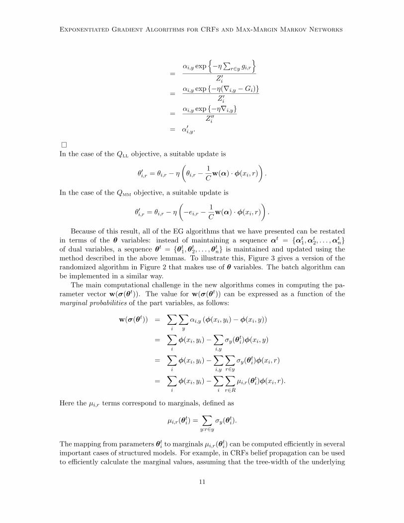
Because of this result, all of the EG algorithms that we have presented can be restatedin terms of the θ variables: instead of maintaining a sequence αt = {αt1,αt2, . . . ,αtn}of dual variables, a sequence θt = {θt1,θt2, . . . ,θtn} is maintained and updated using themethod described in the above lemmas. To illustrate this, Figure 3 gives a version of therandomized algorithm in Figure 2 that makes use of θ variables. The batch algorithm canbe implemented in a similar way.
The main computational challenge in the new algorithms comes in computing the pa-rameter vector w(σ(θt)). The value for w(σ(θt)) can be expressed as a function of themarginal probabilities of the part variables, as follows:
w(σ(θt)) =∑i
∑y
αi,y (φ(xi, yi)− φ(xi, y))
=∑i
φ(xi, yi)−∑i,y
σy(θti)φ(xi, y)
=∑i
φ(xi, yi)−∑i,y
∑r∈y
σy(θti)φ(xi, r)
=∑i
φ(xi, yi)−∑i
∑r∈R
µi,r(θti)φ(xi, r).
Here the µi,r terms correspond to marginals, defined as
µi,r(θti) =∑y:r∈y
σy(θti).
The mapping from parameters θti to marginals µi,r(θti) can be computed efficiently in severalimportant cases of structured models. For example, in CRFs belief propagation can be usedto efficiently calculate the marginal values, assuming that the tree-width of the underlying
11

Collins, Globerson, Koo, Carreras and Bartlett
Inputs: Examples {(xi, yi)}ni=1, learning rate η > 0.
Initialization: For each i = 1 . . . n, set θ1i to some (possibly different) point in R|R|.
Algorithm:
• Calculatew1 =
∑i
φ(xi, yi)−∑i,y
σy(θ1i )φ(xi, y)
• For t = 1, . . . , T , repeat:
– Choose kt uniformly at random from the set [1, 2, . . . , n]
– For all r ∈ R,
If optimizing QLL: θt+1kt,r
= θtkt,r − η(θtkt,r −
1C
wt · φ(xkt, r))
If optimizing QMM: θt+1kt,r
= θtkt,r − η(−ekt,r −
1C
wt · φ(xkt , r))
– For all i 6= kt, for all r, set θt+1i,r = θti,r.
– Calculate
wt+1 =∑i
φ(xi, yi)−∑i,y
σy(θt+1i )φ(xi, y)
= wt +∑y
σy(θtkt)φ(xkt , y)−
∑y
σy(θt+1kt
)φ(xkt , y)
Output: Final dual parameters θT+1 or primal parameters 1CwT+1.
Figure 3: An implementation of the algorithm in Figure 2 using a part-based representation. Thealgorithm uses variables θi for i = 1 . . . n as a replacement for the dual variables αi inFigure 2.
graph is small. In weighted context-free grammars the inside-outside algorithm can beused to calculate marginals, assuming that set of parts R corresponds to context-free ruleproductions. Once marginals are computed, it is straightforward to compute w(σ(θt)) andthereby implement the part-based EG algorithms.
5. Convergence Results
In this section, we provide convergence results for the EG batch and online algorithmspresented in Section 3. Section 5.1 provides the key results, and the following sections givethe proofs and the technical details.
12

Exponentiated Gradient Algorithms for CRFs and Max-Margin Markov Networks
Batch Algorithm Online Algorithm
QMM
n2
ε |A|∞D[α∗‖α1] nε
(|A|∞D[α∗‖α1] + Q(α1)−Q(α∗)
)QLL n(1 + n|A|∞) log(c1ε ) n(1 + |A|∞) log(c2ε )
Table 1: Each entry shows the amount of computation (measured in terms of the num-ber of training sample processed using the EG updates) required to obtainE [|Q(α)−Q(α∗)|] ≤ ε for a given ε > 0. The constants are c1 = (1 +n|A|∞)D[α∗‖α1], and c2 =
[(1 + |A|∞)D[α∗‖α1] +Q(α1)−Q(α∗))
].
5.1 Main Convergence Results
Our convergence results give bounds on how quickly the error |Q(α) − Q(α∗)| decreaseswith respect to the number of iterations, T , of the algorithms. In all cases we have|Q(α) − Q(α∗)| → 0 as T →∞.
In what follows we use D[p‖q] to denote the KL divergence between p,q ∈ ∆n (seeSection 5.2). We also use |A|∞ to denote the maximum magnitude element of A (i.e., |A|∞ =max(i,y),(j,z) |A(i,y),(j,z)|). The first theorem provides results for the EG-batch algorithms,and the second for the randomized online algorithms.
Theorem 1 For the batch algorithm in Figure 1, for QLL and QMM,
Q(α∗) ≤ Q(αT+1) ≤ Q(α∗) +1ηT
D[α∗‖α1] (14)
assuming that the learning rate η satisfies 0 < η ≤ 11+n|A|∞ for QLL, and 0 < η ≤ 1
n|A|∞ forQMM. Furthermore, for QLL,
Q(α∗) ≤ Q(αT+1) ≤ Q(α∗) +e−ηT
ηD[α∗‖α1] (15)
assuming again that 0 < η ≤ 11+n|A|∞ .
The randomized online algorithm will produce different results at every run, since dif-ferent points will be processed on different runs. Our main result for this algorithm char-acterizes the mean value of the objective Q(αT+1) when averaged over all possible randomorderings of points. The result implies that this mean will converge to the optimal valueQ(α∗).
Theorem 2 For the randomized algorithm in Figure 2, for QLL and QMM,
Q(α∗) ≤ E[Q(αT+1)
]≤ Q(α∗) +
n
ηTD[α∗‖α1] +
n
T
[Q(α1)−Q(α∗)
](16)
assuming that the learning rate η satisfies 0 < η ≤ 11+|A|∞ for QLL, and 0 < η ≤ 1
|A|∞ forQMM. Furthermore, for QLL, for the algorithm in Figure 2,
Q(α∗) ≤ E[Q(αT+1)
]≤ Q(α∗) + e−
ηTn
[1ηD[α∗‖α1] +Q(α1)−Q(α∗)
](17)
13

Collins, Globerson, Koo, Carreras and Bartlett
assuming again that 0 < η ≤ 11+|A|∞ .
The above result characterizes the average behavior of the randomized algorithm, butdoes not provide guarantees for any specific run of the algorithm. However, by applyingthe standard approach of repeated sampling (see, for example, Mitzenmacher and Upfal,2005; Shalev-Shwartz et al., 2007), one can obtain a solution that, with high probability,does not deviate by much from the average behavior. In what follows, we briefly outlinethis derivation.
Note that the random variable Q(αT+1) − Q(α∗) is nonnegative, and so by Markov’sinequality, it satisfies
Pr{Q(αT )−Q(α∗) ≥ 2
(E[Q(αT )
]−Q(α∗)
)}≤ 1
2.
Given some δ > 0, if we run the algorithm k = log2(1δ ) times7, each time with T iterations,
and choose the best α of these k results, we see that
Pr{Q(α)−Q(α∗) ≥ 2
(E[Q(αT )
]−Q(α∗)
)}≤ δ.
Thus, for any desired confidence 1−δ, we can obtain a solution that is within a factor of 2 ofthe bound for T iterations in Theorem 2 by using T log2(1
δ ) iterations. In our experiments,we found that repeated trials of the randomized algorithm did not yield significantly differentresults.
The first consequence of the two theorems above is that the batch and randomized onlinealgorithms converge to an α with the optimal value Q(α∗). This follows since Equations14 and 16 imply that as T →∞ the value of Q(αT+1) approaches Q(α∗).
The second consequence is that we can find the number of iterations that the algorithmswill take to reach an α such that E [|Q(α)−Q(α∗)|] ≤ ε for a given ε > 0 (the expectedvalue is redundant for the batch algorithm). Table 1 shows the computation required bythe different algorithms, where the computation is measured by the number of trainingexamples that need to be processed using the EG updates.8 The entries in the table assumethat the maximum possible learning rates are used for each of the algorithms—that is,
11+n|A|∞ for LLEG-Batch, 1
1+|A|∞ for LLEG-Online, 1n|A|∞ for MMEG-batch, and 1
|A|∞ forMMEG-Online.
Crucially, note that these rates suggest that the online algorithms are significantly moreefficient than the batch algorithms; specifically, the bounds suggest that the online algo-rithms require a factor of n less computation in both the QLL and QMM cases. Thus theseresults suggest that the randomized online algorithm should converge much faster than thebatch algorithm. Roughly speaking, this is a direct consequence of the learning rate η beinga factor of n larger in the online case (see also Section 9). This prediction is confirmed inour empirical evaluations, which show that the online algorithm is far more efficient thanthe batch algorithm.
7. Assume for simplicity that log2( 1δ) is integral.
8. Note that if we run the batch algorithm for T iterations (as in the figure), nT training examples areprocessed. In contrast, running the online algorithm for T iterations (again, as shown in the figure) onlyrequires T training examples to be processed. It is important to take this into account when comparingthe rates in Theorems 1 and 2; this is the motivation for measuring computation in terms of the numberof examples that are processed.
14
Exponentiated Gradient Algorithms for CRFs and Max-Margin Markov Networks
A second important point is that the rates for QLL lead to an O(log(1ε )) dependence on
the desired accuracy ε, which is a significant improvement over QMM, which has an O(1ε )
dependence. Note that the O(1ε ) dependence for QMM has been shown for several other
algorithms in the literature (e.g., see Shalev-Shwartz et al., 2007).To gain further intuition into the order of magnitude of iterations required, note that
the factor D[α∗‖α1] which appears in the above expressions is at most n log |Y|, which canbe achieved by setting α1
i to be the uniform distribution over Y for all i. Also, the value of|A|∞ can easily be seen to be 1
C maxi,y ‖ψi,y‖2.In the remainder of this section we give proofs of the results in Theorems 1 and 2. In
doing so, we also give theorems that apply to the optimization of general convex functionsQ : ∆n → R.
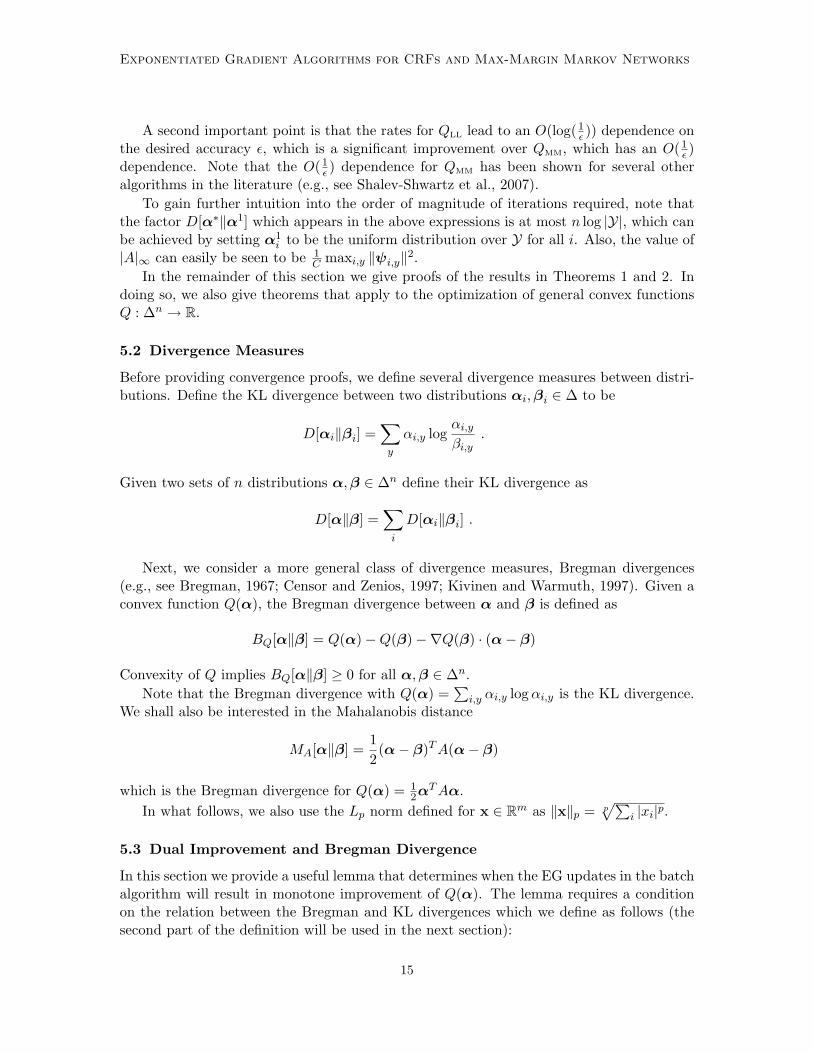
5.2 Divergence Measures
Before providing convergence proofs, we define several divergence measures between distri-butions. Define the KL divergence between two distributions αi,βi ∈ ∆ to be
D[αi‖βi] =∑y
αi,y logαi,yβi,y
.
Given two sets of n distributions α,β ∈ ∆n define their KL divergence as
D[α‖β] =∑i
D[αi‖βi] .
Next, we consider a more general class of divergence measures, Bregman divergences(e.g., see Bregman, 1967; Censor and Zenios, 1997; Kivinen and Warmuth, 1997). Given aconvex function Q(α), the Bregman divergence between α and β is defined as
BQ[α‖β] = Q(α)−Q(β)−∇Q(β) · (α− β)
Convexity of Q implies BQ[α‖β] ≥ 0 for all α,β ∈ ∆n.Note that the Bregman divergence with Q(α) =
∑i,y αi,y logαi,y is the KL divergence.
We shall also be interested in the Mahalanobis distance
MA[α‖β] =12
(α− β)TA(α− β)
which is the Bregman divergence for Q(α) = 12α
TAα.In what follows, we also use the Lp norm defined for x ∈ Rm as ‖x‖p = p
√∑i |xi|p.
5.3 Dual Improvement and Bregman Divergence
In this section we provide a useful lemma that determines when the EG updates in the batchalgorithm will result in monotone improvement of Q(α). The lemma requires a conditionon the relation between the Bregman and KL divergences which we define as follows (thesecond part of the definition will be used in the next section):
15

Collins, Globerson, Koo, Carreras and Bartlett
Definition 5.1 : A convex function Q : ∆n → R is τ -upper-bounded for some τ > 0 if forany p,q ∈ ∆n,
BQ[p‖q] ≤ τD[p‖q].
In addition, we say Q(α) is (µ, τ)-bounded for constants 0 < µ < τ if for any p,q ∈ ∆n,
µD[p‖q] ≤ BQ[p‖q] ≤ τD[p‖q].
The next lemma states that if Q(α) is τ -upper-bounded, then the change in the objectiveas a result of an EG update can be related to the KL divergence between consecutive valuesof the dual variables.
Lemma 2 If Q(α) is τ -upper-bounded, then if η is chosen such that 0 < η ≤ 1τ , it holds
that for all t in the batch algorithm (Figure 1):
Q(αt)−Q(αt+1) ≥ 1ηD[αt‖αt+1] (18)
Proof: Given an αt, the EG update is
αt+1i,y =
1Ztiαti,ye
−η∇ti,y
where
∇ti,y =∂Q(αt)∂αi,y
, Zti =∑y
αti,ye−η∇ti,y
Simple algebra yields∑i
(D[αti‖αt+1
i ] +D[αt+1i ‖α
ti])
= η∑i,y
(αti,y − αt+1i,y )∇ti,y
Equivalently, using the notation for KL divergence between multiple distributions:
D[αt‖αt+1] +D[αt+1‖αt] = η(αt −αt+1) · ∇Q(αt)
The definition of the Bregman divergence BQ then implies
−ηBQ[αt+1‖αt] +D[αt‖αt+1] +D[αt+1‖αt] = η(Q(αt)−Q(αt+1)) (19)
Since Q(α) is τ -upper-bounded and η ≤ 1τ it follows that D[αt+1‖αt] ≥ ηBQ[αt+1‖αt], and
together with Eq. 19 we obtain the desired result η(Q(αt)−Q(αt+1)) ≥ D[αt‖αt+1].
Note that the condition in the lemma may be weakened to requiring that τD[αt‖αt+1] ≥BQ[αt‖αt+1] for all t. For simplicity, we require the condition for all p,q ∈ ∆n. Note alsothat D[p‖q] ≥ 0 for all p,q ∈ ∆n, so the lemma implies that for an appropriately chosenη, the EG updates always decrease the objective Q(α). We next show that the log-lineardual QLL(α) is in fact τ -upper-bounded.
16

Exponentiated Gradient Algorithms for CRFs and Max-Margin Markov Networks
Lemma 3 Define |A|∞ to be the maximum magnitude of any element of A, i.e., |A|∞ =max(i,y),(j,z) |A(i,y),(j,z)|. Then QLL(α) is τLL-upper-bounded with τLL = 1 + n|A|∞.
Proof: First notice that the Bregman divergence BQ is linear in Q. Thus, we can writeBQLL
as a sum of two terms (see Eq. 9).
BQLL[p‖q] = D[p‖q] +MA[p‖q].
We first boundMA[p‖q] in terms of squared L1 distance between p and q. Denote r = p−q.Then:
MA[p‖q] =12
∑i,y,j,z
ri,yrj,zA(i,y),(j,z) ≤|A|∞
2
∑i,y,j,z
|ri,y||rj,z| =|A|∞
2‖p− q‖21. (20)
Next, we use the inequality D[p1‖p2] ≥ 12‖p1− p2‖21 (also known as Pinsker’s inequality, see
Cover and Thomas, 1991, p. 300), which holds for any two distributions p1 and p2. Considerthe two distributions p = 1
np and q = 1nq, each defined over an alphabet of size n|Y|. Then
it follows that:9
|A|∞2‖p− q‖21 =
n2|A|∞2‖p− q‖21 ≤ n2|A|∞D[p‖q] = n|A|∞D[p‖q] (21)
and thus MA[p‖q] ≤ n|A|∞D[p‖q]. So for the Bregman divergence of QLL(α) we obtain
BQLL[p‖q] ≤ (1 + n|A|∞)D[p‖q]
yielding the desired result.
The next lemma shows that a similar result can be obtained for the QMM objective.
Lemma 4 The function QMM(α) is τMM-upper-bounded with τMM = n|A|∞.
Proof: For QMM defined in Eq. 11, we have
BQMM[p‖q] = MA[p‖q]
We can then use a similar derivation to that of Lemma 3 to obtain the result.
We thus have that the condition in Lemma 2 is satisfied for both the QLL(α) andQMM(α) objectives, implying that their EG updates result in monotone improvement of theobjective, for a suitably chosen η:
Corollary 1 The LLEG-Batch algorithm with 0 < η ≤ 1τLL
satisfies for all t
QLL(αt)−QLL(αt+1) ≥ 1ηD[αt‖αt+1] (22)
and the MMEG-Batch algorithm with 0 < η ≤ 1τMM
satisfies for all t
QMM(αt)−QMM(αt+1) ≥ 1ηD[αt‖αt+1] . (23)
9. Note that D[p‖q] is a divergence between two distributions over |Y|n symbols and D[p‖q] is a divergencebetween two sets of n distributions over |Y| symbols.
17
Collins, Globerson, Koo, Carreras and Bartlett
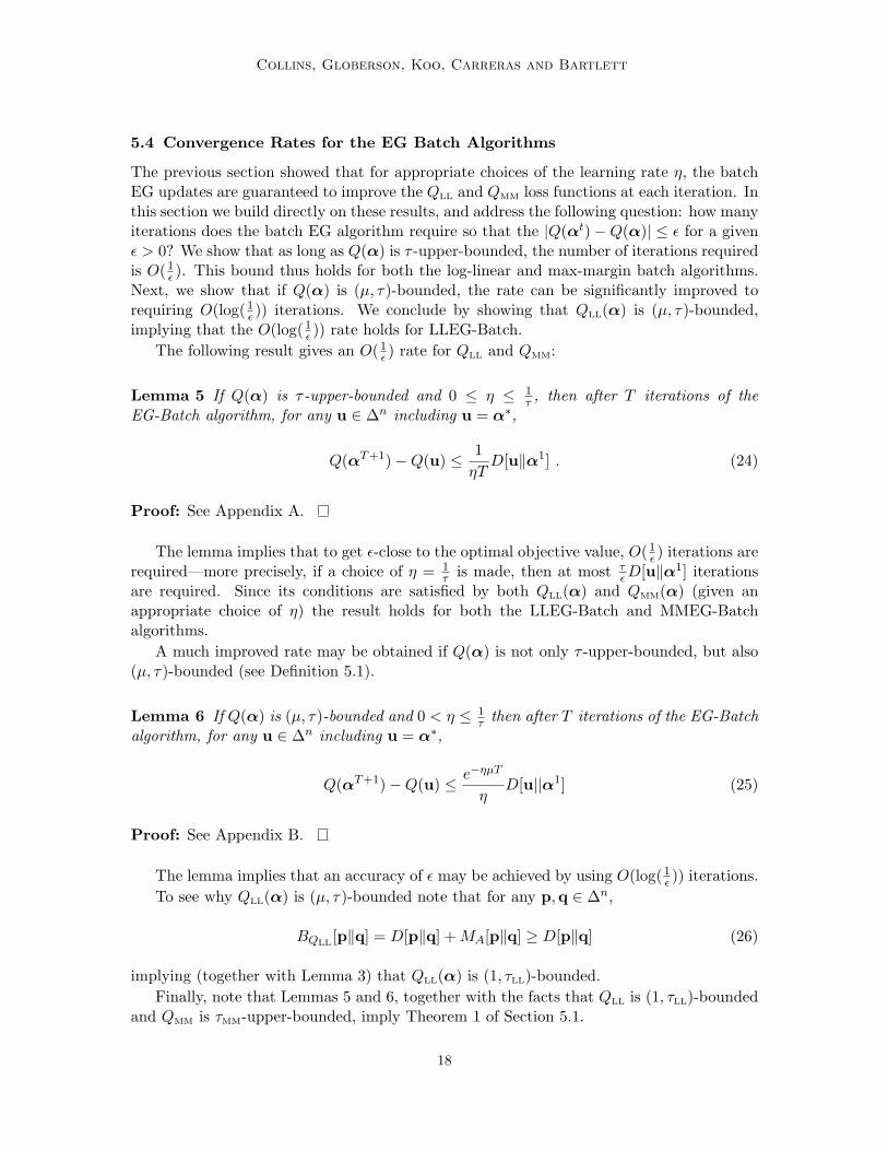
5.4 Convergence Rates for the EG Batch Algorithms
The previous section showed that for appropriate choices of the learning rate η, the batchEG updates are guaranteed to improve the QLL and QMM loss functions at each iteration. Inthis section we build directly on these results, and address the following question: how manyiterations does the batch EG algorithm require so that the |Q(αt)−Q(α)| ≤ ε for a givenε > 0? We show that as long as Q(α) is τ -upper-bounded, the number of iterations requiredis O(1
ε ). This bound thus holds for both the log-linear and max-margin batch algorithms.Next, we show that if Q(α) is (µ, τ)-bounded, the rate can be significantly improved torequiring O(log(1
ε )) iterations. We conclude by showing that QLL(α) is (µ, τ)-bounded,implying that the O(log(1
ε )) rate holds for LLEG-Batch.The following result gives an O(1
ε ) rate for QLL and QMM:
Lemma 5 If Q(α) is τ -upper-bounded and 0 ≤ η ≤ 1τ , then after T iterations of the
EG-Batch algorithm, for any u ∈ ∆n including u = α∗,
Q(αT+1)−Q(u) ≤ 1ηT
D[u‖α1] . (24)
Proof: See Appendix A.
The lemma implies that to get ε-close to the optimal objective value, O(1ε ) iterations are
required—more precisely, if a choice of η = 1τ is made, then at most τ
εD[u‖α1] iterationsare required. Since its conditions are satisfied by both QLL(α) and QMM(α) (given anappropriate choice of η) the result holds for both the LLEG-Batch and MMEG-Batchalgorithms.
A much improved rate may be obtained if Q(α) is not only τ -upper-bounded, but also(µ, τ)-bounded (see Definition 5.1).
Lemma 6 If Q(α) is (µ, τ)-bounded and 0 < η ≤ 1τ then after T iterations of the EG-Batch
algorithm, for any u ∈ ∆n including u = α∗,
Q(αT+1)−Q(u) ≤ e−ηµT
ηD[u||α1] (25)
Proof: See Appendix B.
The lemma implies that an accuracy of ε may be achieved by using O(log(1ε )) iterations.
To see why QLL(α) is (µ, τ)-bounded note that for any p,q ∈ ∆n,
BQLL[p‖q] = D[p‖q] +MA[p‖q] ≥ D[p‖q] (26)
implying (together with Lemma 3) that QLL(α) is (1, τLL)-bounded.Finally, note that Lemmas 5 and 6, together with the facts that QLL is (1, τLL)-bounded
and QMM is τMM-upper-bounded, imply Theorem 1 of Section 5.1.
18
Exponentiated Gradient Algorithms for CRFs and Max-Margin Markov Networks
5.5 Convergence Results for the Randomized Online Algorithm
This section analyzes the rate of convergence of the randomized online algorithm in Figure 2.Before stating the results, we need some definitions. We will use Qα,i : ∆ → R to be thefunction defined as
Qα,i(β) = Q(α1,α2, . . . ,αi−1,β,αi+1, . . . ,αn)
for any β ∈ ∆. We denote the Bregman divergence associated with Qα,i as BQα,i [x‖y]. Wethen introduce the following definitions:
Definition 5.2 : A convex function Q : ∆n → R is τ -online-upper-bounded for some τ > 0if for any i ∈ 1 . . . n and for any p,q ∈ ∆,
BQα,i [p‖q] ≤ τD[p‖q].
In addition, Q is (µ, τ)-online-bounded for 0 < µ < τ if Q is τ -online-upper-bounded, andin addition, for any p,q ∈ ∆n,
µD[p‖q] ≤ BQ[p‖q]
Note that the lower bound in the above definition refers to Q and not to Qα,i. Also, notethat if a function is (µ, τ)-online-bounded then it must also be τ -online-upper-bounded.
The following lemma then gives results for the QLL and QMM functions:
Lemma 7 The regularized log-likelihood dual QLL(α) is (µ, τ)-online-bounded for µ = 1and τ = 1 + |A|∞. The max-margin dual QMM(α) is τ -online-upper-bounded for τ = |A|∞.
Proof: See Appendix C.
For any (µ, τ)-online-bounded Q, the online EG algorithm converges at an exponentialrate, as shown by the following lemma.
Lemma 8 Consider the algorithm in Figure 2 applied to a convex function Q(α) that is(µ, τ)-online-bounded. If η > 0 is chosen such that η ≤ 1
τ , then it follows that for all u ∈ ∆n
E[Q(αT+1)
]≤ Q(u) + e−
ηµTn
[1ηD[u‖α1] +Q(α1)−Q(α∗)
](27)
where α∗ = argminα∈∆n Q(α).
Proof: See Appendix D.
The previous lemma shows, in particular, that the online EG algorithm converges at anexponential rate for the function QLL. However, these results do not apply to QMM, whichis only τ -online-upper-bounded. The following lemma shows that such functions exhibit aO( 1
T ) rate of convergence.
19

Collins, Globerson, Koo, Carreras and Bartlett
Lemma 9 Consider the algorithm in Figure 2 applied to a convex function Q(α) that isτ -online-upper-bounded. If η > 0 is chosen such that η ≤ 1
τ , then it follows that for allu ∈ ∆n
E[Q(αT+1)
]≤ Q(u) +
n
ηTD[u‖α1] +
n
T
[Q(α1)−Q(α∗)
](28)
where E[Q(αT+1)
]is the expected value of Q(αT+1), and α∗ = argminα∈∆n Q(α).
Proof: See Appendix E.
Note that Lemmas 7, 8 and 9 complete the proof of Theorem 2 in Section 5.1.
6. Related Work
The idea of solving regularized loss-minimization problems via their convex duals has beenaddressed in several previous papers. Here we review those, specifically focusing on thelog-linear and max-margin problems.
Zhang (2002) presented a study of convex duals of general regularized loss functions,and provided a methodology for deriving such duals. He also considered a general procedurefor solving such duals by optimizing one coordinate at a time. However, it is not clear howto implement this procedure in the structured learning case (i.e., when |Y| is large), andconvergence rates are not given.
In the specific context of log-linear models, several works have studied dual optimization.Earlier work (Jaakkola and Haussler, 1999; Keerthi et al., 2005; Zhu and Hastie, 2001)treated the logistic regression model, a simpler version of a CRF. In the binary logisticregression case, there is essentially one parameter αi with the constraint 0 ≤ αi ≤ 1 andtherefore simple line search methods can be used for optimization. Minka (2003) showsempirical results which show that this approach performs similarly to conjugate gradient.The problem becomes much harder when αi is constrained to be a distribution over manylabels, as in the case discussed here. Recently, Memisevic (2006) addressed this setting,and suggests optimizing αi by transferring probability mass between two labels y1, y2 whilekeeping the distribution normalized. This requires a strategy for choosing these two labels,and the author suggests one which seems to perform well. We note that our EG updateschange the whole distribution αi and are thus expected to yield much better improvementof the objective.
While some previous work on log-linear models proved convergence of dual methods (e.g.,Keerthi et al., 2005), we are not aware of rates of convergence that have been reported inthis context. Convergence rates for related algorithms, in particular a generalization of EG,known as the Mirror-Descent algorithm, have been studied in a more general context in theoptimization literature. For instance, Beck and Teboulle (2003) describe convergence resultswhich apply to quite general definitions of Q(α), but which have only O( 1
ε2) convergence
rates, as compared to our results of O(1ε ) and O(log(1
ε )) for the max-margin and log-linearcases respectively. Also, their work considers optimization over a single simplex, and doesnot consider online-like algorithms such as the one we have presented.
For max-margin models, numerous dual methods have been suggested, an earlier ex-ample being the SMO algorithm of Platt (1998). Such methods optimize subsets of the αparameters in the dual SVM formulation (see also Crammer and Singer, 2002). Analysis
20

Exponentiated Gradient Algorithms for CRFs and Max-Margin Markov Networks
of a similar algorithm (Hush et al., 2006) results in an O(1ε ) rate, similar to the one we
have here. Another algorithm for solving SVMs via the dual is the multiplicative updatemethod of Sha et al. (2007). These updates are shown to converge to the optimum of theSVM dual, but convergence rate has not been analyzed, and extension to the structuredcase seems non-trivial. An application of EG to binary SVMs was previously studied byCristianini et al. (1998). They show convergence rates of O( 1
ε2), that are slower than our
O(1ε ), and no extension to structured learning (or multi-class) is discussed.Recently, several new algorithms have been presented, along with a rate of convergence
analysis (Joachims, 2006; Shalev-Shwartz et al., 2007; Teo et al., 2007; Tsochantaridis et al.,2004). All of these algorithms are similar to ours in having a relatively low dependence on nin terms of memory and computation. Among these, Shalev-Shwartz et al. (2007) and Teoet al. (2007), present an O(1
ε ) rate, but where accuracy is measured in the primal or via theduality gap, and not in the dual as in our analysis. Thus, it seems that a rate of O(1
ε ) iscurrently the best known result for algorithms that have a relatively low dependence on n(general QP solvers, which may have O(log(1
ε )) behavior, generally have a larger dependenceon n, both in time and space).
7. Experiments on Regularized Log-Likelihood
In this section we analyze the performance of the EG algorithms for optimization of reg-ularized log-likelihood. We describe experiments on two tasks: first, the MNIST digitclassification task, which is a multiclass classification task; second, a log-linear model for astructured natural-language dependency-parsing task. In each case we first give results forthe EG method, and then compare its performance to L-BFGS (Byrd et al., 1995), whichis a batch gradient descent method, and to stochastic gradient descent.10
We do not report results on LLEG-Batch, since we found it to converge much moreslowly than the online algorithm. This is expected from our theoretical results, whichanticipate a factor of n speed-up for the online algorithm. We also report experimentscomparing the randomized online algorithm to a deterministic online EG algorithm, wheresamples are drawn in a fixed order (e.g., the algorithm first visits the first example, thenthe second, etc.).
Although EG is guaranteed to converge for an appropriately chosen η, it turns out tobe beneficial to use an adaptive learning rate. Here we use the following crude strategy:we first consider only 10% of the data-set, and find a value of η that results in monotoneimprovement for at least 95% of the samples. Denote this value by ηini (for the experimentsin Section 7.1 we simply use ηini = 0.5). For learning over the entire data-set, we keep alearning rate ηi for each sample i (where i = 1, . . . , n), and initialize this rate to ηini forall points. When sample i is visited, we halve ηi until an improvement in the objective isobtained. Finally, after the update, we multiply ηi by 1.05, so that it does not decreasemonotonically.
It is important that when updating a single example using the online algorithms, theimprovement (or decrease) in the dual can be easily evaluated, allowing the halving strategydescribed in the previous paragraph to be implemented efficiently. If the current dual
10. We also experimented with conjugate gradient algorithms, but since these resulted in worse performancethan L-BFGS, we do not report these results here.
21

Collins, Globerson, Koo, Carreras and Bartlett
parameters are α, the i’th coordinate is selected, and the EG updates then map αi to α′i,the change in the dual objective is
∑y
α′i,y logα′i,y +1
2C
∥∥∥∥∥w(α) +∑y
(α′i,y − αi,y
)ψi,y
∥∥∥∥∥2
−∑y
αi,y logαi,y −1
2C‖w(α)‖2
The primal parameters w(α) are maintained throughout the algorithm (see Figure 3), sothat this change in the dual objective can be calculated efficiently. A similar method canbe used to calculate the change in the dual objective in the max-margin case.
We measure the performance of each training algorithm (the EG algorithms, as wellas the batch gradient and stochastic gradient methods) as a function of the amount ofcomputation spent. Specifically, we measure computation in terms of the number of timeseach training example is visited. For EG, an example is considered to be visited for everyvalue of η that is tested on it. For L-BFGS, all examples are visited for every evaluationperformed by the line-search routine. We define the measure of effective iterations to bethe number of examples visited, divided by n.
7.1 Multi-class Classification
We first conducted multi-class classification experiments on the MNIST classification task.Examples in this dataset are images of handwritten digits represented as 784-dimensionalvectors. We used a training set of 59k examples, and a validation set of 10k examples.11
We define a ten-class logistic-regression model where
p(y |x) ∝ ex·wy (29)
and x,wy ∈ R784, y ∈ {1, . . . , 10}.Models were trained for various values of the regularization parameter C: specifically, we
tried values of C equal to 1000, 100, 10, 1, 0.1, and 0.01. Convergence of the EG algorithmfor low values of C (i.e., 0.1 and 0.01) was found to be slow; we discuss this issue more inSection 7.1.1, arguing that it is not a serious problem.
Figure 4 shows plots of the validation error versus computation for C equal to 1000,100, 10, and 1, when using the EG algorithm. For C equal to 10 or more, convergence isfast. For C = 1 convergence is somewhat slower. Note that there is little to choose betweenC = 10 and C = 1 in terms of validation error.
Figure 5 shows plots of the primal and dual objective functions for different values of C.Note that EG does not explicitly minimize the primal objective function, so the EG primalwill not necessarily decrease at every iteration. Nevertheless, our experiments show thatthe EG primal decreases quite quickly. Figure 6 shows how the duality gap decreases withthe amount of computation spent (the duality gap is the difference between the primal anddual values at each iteration). The log of the duality gap decreases more-or-less linearlywith the amount of computation spent, as predicted by the O(log(1
ε )) bounds on the rateof convergence.
11. In reporting results, we consider only validation error; that is, error computed during the training processon a validation set. This measure is often used in early-stopping of algorithms, and is therefore of interestin the current context. We do not report test error since our main focus is algorithmic.
22

Exponentiated Gradient Algorithms for CRFs and Max-Margin Markov Networks
7
8
9
10
11
12
13
14
15
16
10 20 30 40 50 60 70 80 90 100
Cla
ssifi
catio
n E
rror
(%
)
Eff. Iteration
C=1C=10C=100C=1000
7.2
7.3
7.4
7.5
7.6
7.7
7.8
7.9
8
20 40 60 80 100 120 140 160 180 200
Cla
ssifi
catio
n E
rror
(%
)
Eff. Iteration
C=1C=10
Figure 4: Validation error results on the MNIST learning task for log-linear models trained usingthe EG randomized online algorithm. The X axis shows the number of effective iterationsover the entire data set. The Y axis shows validation error percentages. The left figureshows plots for values of C equal to 1, 10, 100, and 1000. The right figure shows plotsfor C equal to 1 and 10 at a larger scale.
Finally, we compare the deterministic and randomized versions of the EG algorithm.Figure 7 shows the primal and dual objectives for both algorithms. It can be seen that therandomized algorithm is clearly much faster to converge. This is even more evident whenplotting the duality gap, which converges much faster to zero in the case of the randomizedalgorithm. These results give empirical evidence that the randomized strategy is to bepreferred over a fixed ordering of the training examples (note that we have been able toprove bounds on convergence rate for the randomized algorithm, but have not been able toprove similar bounds for the deterministic case).
7.1.1 Convergence for Low Values of C
As mentioned in the previous section, convergence of the EG algorithm for low values of Ccan be very slow. This is to be expected from the bounds on convergence, which predict thatconvergence time should scale linearly with 1
C (other algorithms, e.g., see Shalev-Shwartzet al., 2007, also require O( 1
C ) time for convergence). This is however, not a serious problemon the MNIST data, where validation error has reached a minimum point for around C = 10or C = 1.
If convergence for small values of C is required, one strategy we have found effective isto start C at a higher value, then “anneal” it towards the target value. For example, seeFigure 8 for results for C = 1 using one such annealing scheme. For this experiment, if wetake t to be number of iterations over the training set, where for any t we have processedt × n training examples, we set C = 10 for t ≤ 5, and set C = 1 + 9 × 0.7t−5 for t > 5.Thus C starts at 10, then decays exponentially quickly towards the target value of 1. It
23

Collins, Globerson, Koo, Carreras and Bartlett
0
0.2
0.4
0.6
0.8
1
5 10 15 20 25 30 35 40 45 50
Obj
ectiv
e
Eff. Iteration
Primal, C=1000Dual, C=1000Primal, C=100Dual, C=100
0
0.1
0.2
0.3
0.4
0.5
0.6
5 10 15 20 25 30 35 40 45 50
Obj
ectiv
e
Eff. Iteration
Primal, C=10Dual, C=10Primal, C=1Dual, C=1
Figure 5: Primal and dual objective values on the MNIST learning task for log-linear models trainedusing the EG randomized online algorithm. The dual values have been negated so thatthe primal and dual problems have the same optimal value. The X axis shows the numberof effective iterations over the entire data set. The Y axis shows the value of the primalor dual objective functions. The left figure shows plots for values of C equal to 1000 and100; the right figure shows plots for C equal to 10, and 1. In all cases the primal anddual objectives converge to the same value, with faster convergence for larger values ofC.
can be seen that convergence is significantly faster for the annealed method. The intuitionbehind this method is that the solution to the dual problem for C = 10 is a reasonableapproximation to the solution for C = 1, and is considerably more easy to solve; in theannealing strategy we start with an easier problem and then gradually move towards theharder problem of C = 1.
7.1.2 An Efficient Method for Optimizing a Range of C Values
In practice, when estimating parameters using either regularized log-likelihood or hinge-loss, a range of values for C are tested, with cross-validation or validation on a held-outset being used to choose the optimal value of C. In the previously described experiments,we independently optimized log-likelihood-based models for different values of C. In thissection we describe a highly efficient method for training a sequence of models for a rangeof values of C.
The method is as follows. We pick some maximum value for C; as in our previousexperiments, we will choose a maximum value of C = 1000. We also pick a tolerance valueε, and a parameter 0 < β < 1. We then optimize C using the randomized online algorithm,until the duality gap is less than ε×p, where p is the primal value. Once the duality gap hasconverged to within this ε tolerance, we reduce C by a factor of β, and again optimize towithin an ε tolerance. We continue this strategy—for each value of C optimizing to withina factor of ε, then reducing C by a factor of β—until C has reached a low enough value. At
24

Exponentiated Gradient Algorithms for CRFs and Max-Margin Markov Networks
1e-04
0.001
0.01
0.1
1
10
100
20 40 60 80 100 120 140 160 180 200
Dua
lity
Gap
(%
)
Eff. Iteration
C=1000C=100C=10C=1
Figure 6: Graph showing the duality gap on the MNIST learning task for log-linear models trainedusing the EG randomized online algorithm. The X axis shows the number of effectiveiterations over the entire data set. The Y axis (with a log scale) shows the value of theduality gap, as a percentage of the final optimal value.
0
0.1
0.2
0.3
0.4
0.5
0.6
0.7
0 50 100 150 200 250
Obj
ectiv
e
Eff. Iteration
Primal - Deterministic EGDual - Deterministic EGPrimal - Randomized EGDual - Randomized EG
0
50
100
150
200
250
0 50 100 150 200 250
Dua
lity
Gap
(%
)
Eff. Iteration
Deterministic EGRandomized EG
Figure 7: Results on the MNIST learning task, comparing the randomized and deterministic onlineEG algorithms, for C = 1. The left figure shows primal and dual objective valuesfor both algorithms. The right figure shows the normalized value of the duality gap:(primal(t)− dual(t))/opt, where opt is the value of the joint optimum of the primal anddual problems, and t is the iteration number. The X axis counts the number of effectiveiterations over the entire data set.
the end of the sequence, this method recovers a series of models for different values of C,each optimized to within a tolerance of ε.
25
Collins, Globerson, Koo, Carreras and Bartlett
0.2
0.25
0.3
0.35
0.4
0.45
0.5
0.55
0.6
0.65
5 10 15 20 25 30 35 40 45 50
Obj
ectiv
e
Eff. Iteration
C=1C=1, annealed
7
8
9
10
11
12
13
14
15
16
10 20 30 40 50 60 70 80 90 100
Cla
ssifi
catio
n E
rror
(%
)
Eff. Iteration
C=1C=1, annealed
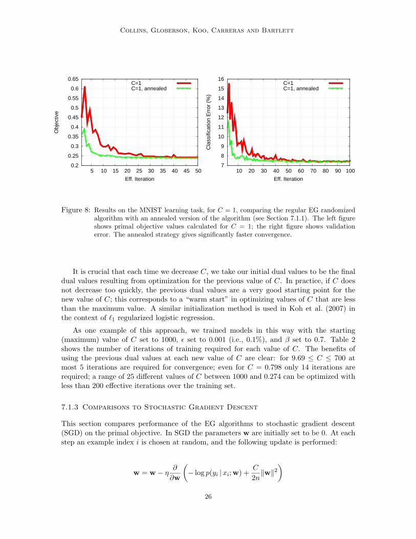
Figure 8: Results on the MNIST learning task, for C = 1, comparing the regular EG randomizedalgorithm with an annealed version of the algorithm (see Section 7.1.1). The left figureshows primal objective values calculated for C = 1; the right figure shows validationerror. The annealed strategy gives significantly faster convergence.
It is crucial that each time we decrease C, we take our initial dual values to be the finaldual values resulting from optimization for the previous value of C. In practice, if C doesnot decrease too quickly, the previous dual values are a very good starting point for thenew value of C; this corresponds to a “warm start” in optimizing values of C that are lessthan the maximum value. A similar initialization method is used in Koh et al. (2007) inthe context of `1 regularized logistic regression.
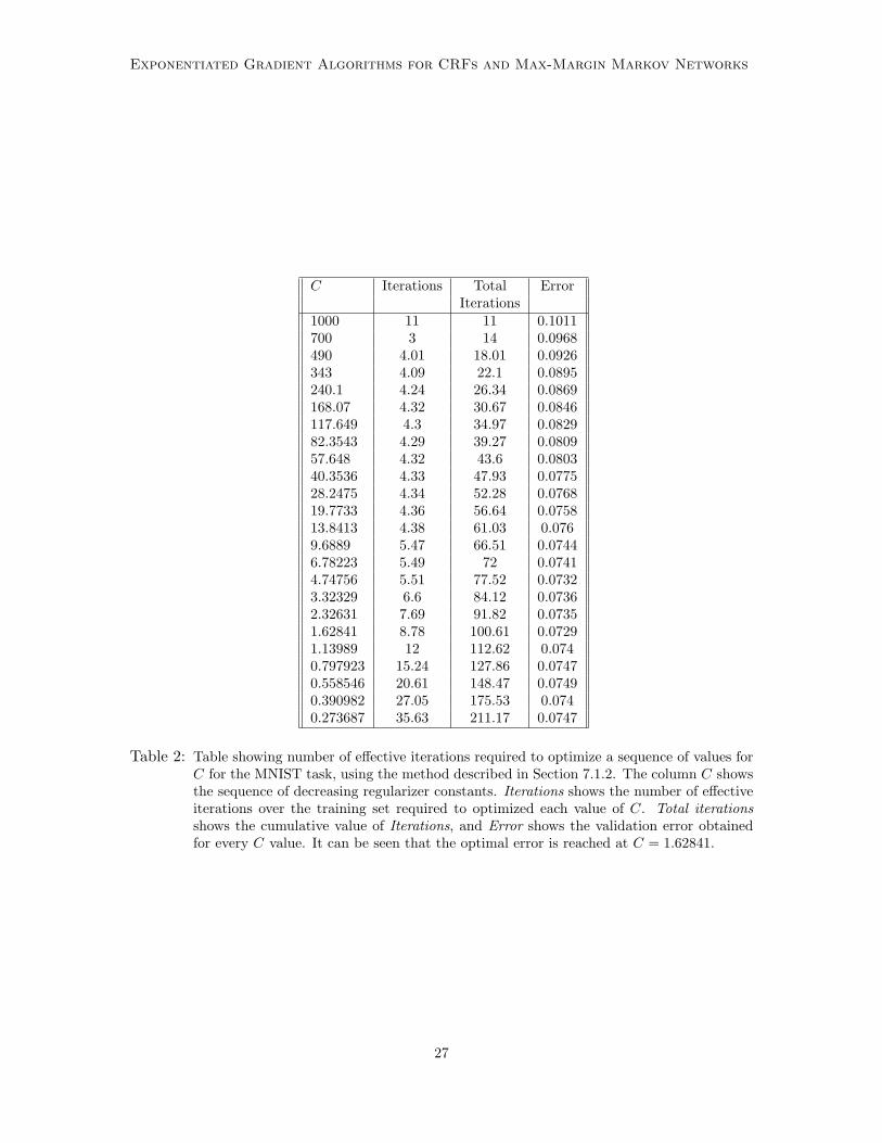
As one example of this approach, we trained models in this way with the starting(maximum) value of C set to 1000, ε set to 0.001 (i.e., 0.1%), and β set to 0.7. Table 2shows the number of iterations of training required for each value of C. The benefits ofusing the previous dual values at each new value of C are clear: for 9.69 ≤ C ≤ 700 atmost 5 iterations are required for convergence; even for C = 0.798 only 14 iterations arerequired; a range of 25 different values of C between 1000 and 0.274 can be optimized withless than 200 effective iterations over the training set.
7.1.3 Comparisons to Stochastic Gradient Descent
This section compares performance of the EG algorithms to stochastic gradient descent(SGD) on the primal objective. In SGD the parameters w are initially set to be 0. At eachstep an example index i is chosen at random, and the following update is performed:
w = w − η ∂
∂w
(− log p(yi |xi; w) +
C
2n‖w‖2
)26
Exponentiated Gradient Algorithms for CRFs and Max-Margin Markov Networks
C Iterations Total ErrorIterations
1000 11 11 0.1011700 3 14 0.0968490 4.01 18.01 0.0926343 4.09 22.1 0.0895240.1 4.24 26.34 0.0869168.07 4.32 30.67 0.0846117.649 4.3 34.97 0.082982.3543 4.29 39.27 0.080957.648 4.32 43.6 0.080340.3536 4.33 47.93 0.077528.2475 4.34 52.28 0.076819.7733 4.36 56.64 0.075813.8413 4.38 61.03 0.0769.6889 5.47 66.51 0.07446.78223 5.49 72 0.07414.74756 5.51 77.52 0.07323.32329 6.6 84.12 0.07362.32631 7.69 91.82 0.07351.62841 8.78 100.61 0.07291.13989 12 112.62 0.0740.797923 15.24 127.86 0.07470.558546 20.61 148.47 0.07490.390982 27.05 175.53 0.0740.273687 35.63 211.17 0.0747
Table 2: Table showing number of effective iterations required to optimize a sequence of values forC for the MNIST task, using the method described in Section 7.1.2. The column C showsthe sequence of decreasing regularizer constants. Iterations shows the number of effectiveiterations over the training set required to optimized each value of C. Total iterationsshows the cumulative value of Iterations, and Error shows the validation error obtainedfor every C value. It can be seen that the optimal error is reached at C = 1.62841.
27

Collins, Globerson, Koo, Carreras and Bartlett
where η > 0 is a learning rate. The term
∂
∂w
(− log p(yi |xi; w) +
C
2n‖w‖2
)can be thought of as an estimate of the gradient of the primal objective function for theentire training set.
In our experiments, we chose the learning rate η to be
η =η0
1 + k/n
where η0 > 0 is a constant, n is the number of training examples, and k is the number ofupdates that have been performed up to this point. Thus the learning rate decays to 0 withthe number of examples that are updated. This follows the approach described in LeCunet al. (1998); we have consistently found that it performs better than using a single, fixedlearning rate.
We tested SGD for C values of 1000, 100, 10, 1, 0.1 and 0.01. In each case we chose thevalue of η0 as follows. For each value of C we first tested values of η0 equal to 1, 0.1, 0.01,0.001, and 0.0001, and then chose the value of η0 which led to the best validation error aftera single iteration of SGD. This strategy resulted in a choice of η0 = 0.01 for all values of Cexcept C = 1000, where η0 = 0.001 was chosen. We have found this strategy to be a robustmethod for choosing η0 (note that we do not want to run SGD for more iterations with all(C, η0) combinations, as this would require 5 times as much computation as picking a singlevalue of η0).
Figure 9 compares validation error rates for SGD and the randomized EG algorithm.For the initial (roughly 5) iterations of training, SGD has better validation error scores, butbeyond this the EG algorithm looks very competitive on this task. Note that the amountof computation for SGD does not include the iterations required to find the optimal valueof η0; if this computation was included the SGD curves would be shifted 5 iterations to theright.
To compare the primal objective obtained by EG and SGD, we used the EG weightvector 1
Cw(αt) to compute primal values. Figure 10 shows graphs comparing performancein optimizing the primal objective value for EG and SGD. For C equal to 1000, 100, and10, the results are similar: SGD is initially better than EG, but after around 5 iterationsEG overtakes SGD, and converges much more quickly to the optimal point. The differencebetween EG and SGD appears to become more pronounced as C becomes smaller. ForC = 1 our strategy for choosing η0 does not pick the optimal value for η0 at least whenevaluating the primal objective; see the caption to the figure for more discussion. EG againappears to out-perform SGD after the initial few iterations.
7.1.4 Comparisons to L-BFGS
One of the standard approaches to training log-linear models is using the L-BFGS gradient-based algorithm (Sha and Pereira, 2003). L-BFGS is a batch algorithm, in the sense thatits updates require evaluating the primal objective and gradient, which involves iterating
28

Exponentiated Gradient Algorithms for CRFs and Max-Margin Markov Networks
7
8
9
10
11
12
10 20 30 40 50 60 70 80 90 100
Cla
ssifi
catio
n E
rror
(%
)
Eff. Iteration
EG, C=10SGD, C=10SGD, C=0.01SGD, C=1000SGD, C=100
7.3
7.4
7.5
7.6
7.7
7.8
7.9
8
5 10 15 20 25 30 35 40 45 50
Cla
ssifi
catio
n E
rror
(%
)
Eff. Iteration
EG, C=10SGD, C=10SGD, C=0.01
Figure 9: Graphs showing validation error results on the MNIST learning task, comparing the EGrandomized algorithm to stochastic gradient descent (SGD). The X axis shows numberof effective training iterations, the Y axis shows validation error in percent. The EGresults are shown for C = 10; SGD results are shown for several values of C. For SGDfor C = 1, C = 0.1, and C = 0.01 the curves were nearly identical, hence we omit thecurves for C = 1 and C = 0.1. Note that the amount of computation for SGD does notinclude the iterations required to find the optimal value for the learning rate η0.
over the entire data-set. To compare L-BFGS to EG, we used the implementation based onByrd et al. (1995).12
For L-BFGS, a total of n training examples must be processed every time the gradient orobjective function is evaluated; note that because L-BFGS uses a line search, each iterationmay involve several such evaluations.13
As in Section 7.1.3, we calculated primal values for EG. Figure 11 shows the primalobjective for EG, and L-BFGS. It can be seen that the primal value for EG convergesconsiderably faster than the L-BFGS one. Also shown is a curve of validation error for bothalgorithms. Here we show the results for EG with C = 10 and L-BFGS with various Cvalues. It can be seen that L-BFGS does not outperform the EG curve for any value of C.
12. Specifically, we used the code by Zhu, Byrd, Lu, and Nocedal’s (www.ece.northwestern.edu/∼nocedal/)with L. Stewart’s wrapper (www.cs.toronto.edu/∼liam/).
13. The implementation of L-BFGS that we use requires both the gradient and objective when performingthe line-search. In some line-search variants, it is possible to use only objective evaluations. In this case,the EG line search will be somewhat more costly, since the dual objective requires evaluations of bothmarginals and partition function, whereas the primal objective only requires the partition function. Thiswill have an effect on running times only if the EG line search evaluates more than one point, whichhappened for less than 10% of the points in our experiments.
29

Collins, Globerson, Koo, Carreras and Bartlett
0.644
0.645
0.646
0.647
0.648
0.649
0.65
0.651
0.652
10 20 30 40 50 60 70 80 90 100
Obj
ectiv
e
Eff. Iteration
EG, C=1000SGD, C=1000
0.37
0.375
0.38
0.385
0.39
0.395
0.4
10 20 30 40 50 60 70 80 90 100
Obj
ectiv
e
Eff. Iteration
EG, C=100SGD, C=100
0.27
0.28
0.29
0.3
0.31
0.32
0.33
0.34
10 20 30 40 50 60 70 80 90 100
Obj
ectiv
e
Eff. Iteration
EG, C=10SGD, C=10
0.24
0.26
0.28
0.3
0.32
0.34
10 20 30 40 50 60 70 80 90 100
Obj
ectiv
e
Eff. Iteration
EG, C=1EG, C=1, annealedSGD, C=1, eta=0.1SGD, C=1, eta=0.01
Figure 10: Graphs showing primal objective values on the MNIST learning task, comparing the EGrandomized algorithm to stochastic gradient descent (SGD). The X axis shows numberof effective training iterations, the Y axis shows primal objective. The graphs are forC equal to 1000, 100, 10, and 1. For C = 1 we show EG results with and withoutthe annealed strategy described in Section 7.1.1. For C = 1 we also show two SGDcurves, for learning rates 0.01 and 0.1: in this case η0 = 0.01 was the best-performinglearning rate after one iteration for both validation error and primal objective, howevera post-hoc analysis shows that η0 = 0.1 converges to a better value in the limit. Thusour strategy for choosing η0 was not optimal in this case, although it is difficult toknow how η0 = 0.1 could be chosen without post-hoc analysis of the convergence forthe different values of η0. For other values of C our strategy for picking η0 was morerobust.
7.2 Structured learning - Dependency Parsing
Parsing of natural language sentences is a challenging structured learning task. Dependencyparsing (McDonald et al., 2005) is a simplified form of parsing where the goal is to map
30

Exponentiated Gradient Algorithms for CRFs and Max-Margin Markov Networks
0.65
0.7
0.75
0.8
5 10 15 20 25 30
Obj
ectiv
e
Eff. Iteration
EG, C=1000L-BFGS, C=1000
0.35
0.4
0.45
0.5
0.55
10 20 30 40 50 60
Obj
ectiv
e
Eff. Iteration
EG, C=100L-BFGS, C=100
0.25
0.3
0.35
0.4
0.45
0.5
10 20 30 40 50 60 70 80 90 100
Obj
ectiv
e
Eff. Iteration
EG, C=10L-BFGS, C=10
0.2
0.25
0.3
0.35
0.4
0.45
0.5
20 40 60 80 100 120 140 160 180 200
Obj
ectiv
e
Eff. Iteration
EG, C=1EG, C=1, annealedL-BFGS, C=1
7
8
9
10
11
12
10 20 30 40 50 60 70 80 90 100
Cla
ssifi
catio
n E
rror
(%
)
Eff. Iteration
EG, C=10L-BFGS, C=1000L-BFGS, C=100 L-BFGS, C=10L-BFGS, C=1L-BFGS, C=0.1L-BFGS, C=0.01
Figure 11: Results on the MNIST learning task, comparing the EG algorithm to L-BFGS. Thefigures on the first and second row show the primal objective for both algorithms, forvarious values of C. The bottom curve shows validation error for L-BFGS for variousvalues of C and for EG with C = 10.
31

Collins, Globerson, Koo, Carreras and Bartlett
sentences x into projective directed spanning trees over the set of words in x. Each labely is a set of directed arcs (dependencies) between pairs of words in the sentence. Eachdependency is a pair (h,m) where h is the index of the head word of the dependency,and m is the index of the modifier word. Assuming we have a function φ(x, h,m) thatassigns a feature vector to dependencies (h,m), we can use a weight vector w to score agiven tree y by w ·
∑(h,m)∈y φ(x, h,m). Dependency parsing corresponds to a structured
problem where the parts r are dependencies (h,m); the approach described in Section 4 canbe applied efficiently to dependency structures. For projective dependency trees (e.g., seeKoo et al., 2007), the required marginals can be computed efficiently using a variant of theinside-outside algorithm (Baker, 1979).
In the experiments below we use a feature set φ(x, h,m) similar to that in McDonaldet al. (2005) and Koo et al. (2007), resulting in 2, 500, 554 features. We report results on theSpanish data-set which is part of the CoNLL-X Shared Task on multilingual dependencyparsing (Buchholz and Marsi, 2006). The training data consists of 2, 306 sentences (58, 771tokens). To evaluate validation error, we use 1, 000 sentences (30, 563 tokens) and reportaccuracy (rate of correct edges in a predicted parse tree) on these sentences.14
As in the multi-class experiments, we compare to SGD and L-BFGS. The implementa-tion of the algorithms is similar to that described in Section 7.1. The gradients for SGDand L-BFGS were obtained by calculating the relevant marginals of the model, using theinside-outside algorithm that was also used for EG. The learning rate for SGD was chosenas in the previous section; that is, we tested several learning rates (η0 = 1, 0.1, 0.001, 0.0001)and chose the one that yielded the minimum validation error after one iteration.
Figure 12 shows results for EG and L-BFGS on the parsing task. We experiment withvalues of C in the set {0.1, 1, 10, 100, 1000}. Of these, the value that results in optimalvalidation error was C = 10. The performance of L-BFGS, SGD and EG is demonstratedin terms of the primal objective for a subset of the C values. L-BFGS and EG bothconverge to the optimal value, and EG is significantly faster. On the other hand, SGDdoes not converge to the optimum for all C values (e.g., for C = 1, 10), and when it doesconverge to the optimum, it is slower than EG.
Figure 12 also shows the validation error for EG at the optimal C value, compared tovalidation error for L-BFGS and SGD at various C values. Again, it can be seen the EGcurve significantly outperforms those of L-BFGS. For SGD, performance is comparable toEG. However, as mentioned earlier, SGD in fact does not successfully optimize the primalobjective for low values of C, and for higher values of C the SGD primal objective is slowerto converge.
As in the multi-class experiments (see Figure 10), it is possible to find learning rates forSGD such that it converges to the primal optimum for C = 1, 10. However, the optimalityof these rates only becomes evident after 10 iterations or more (results not shown). Thus, tofind a learning rate for SGD that actually solves the optimization problem would typicallyrequire an additional few tens of iterations, making it significantly slower than EG.
Finally, it is possible to use EG to efficiently optimize over a set of regularization con-stants, as in Section 7.1.2. Table 3 shows results for a sequence of regularization constants.
14. All 3, 306 sentences were obtained from the training data section of the CoNLL-X Spanish data-set (Civitand Martı, 2002).
32
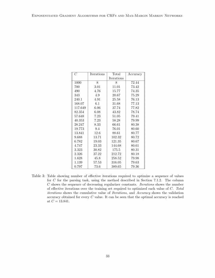
Exponentiated Gradient Algorithms for CRFs and Max-Margin Markov Networks
C Iterations Total AccuracyIterations
1000 8 8 72.44700 3.01 11.01 73.42490 4.76 15.77 74.35343 4.9 20.67 75.29240.1 4.91 25.58 76.13168.07 6.1 31.68 77.13117.649 6.06 37.74 77.8282.354 6.08 43.82 78.7457.648 7.23 51.05 79.4140.353 7.23 58.28 79.9928.247 8.33 66.61 80.3819.773 9.4 76.01 80.6013.841 12.6 88.61 80.779.688 13.71 102.32 80.726.782 19.03 121.35 80.674.747 23.33 144.68 80.613.323 30.82 175.5 80.312.326 37.22 212.72 80.181.628 45.8 258.52 79.981.139 57.53 316.05 79.630.797 73.6 389.65 79.36
Table 3: Table showing number of effective iterations required to optimize a sequence of valuesfor C for the parsing task, using the method described in Section 7.1.2. The columnC shows the sequence of decreasing regularizer constants. Iterations shows the numberof effective iterations over the training set required to optimized each value of C. Totaliterations shows the cumulative value of Iterations, and Accuracy shows the validationaccuracy obtained for every C value. It can be seen that the optimal accuracy is reachedat C = 13.841.
33
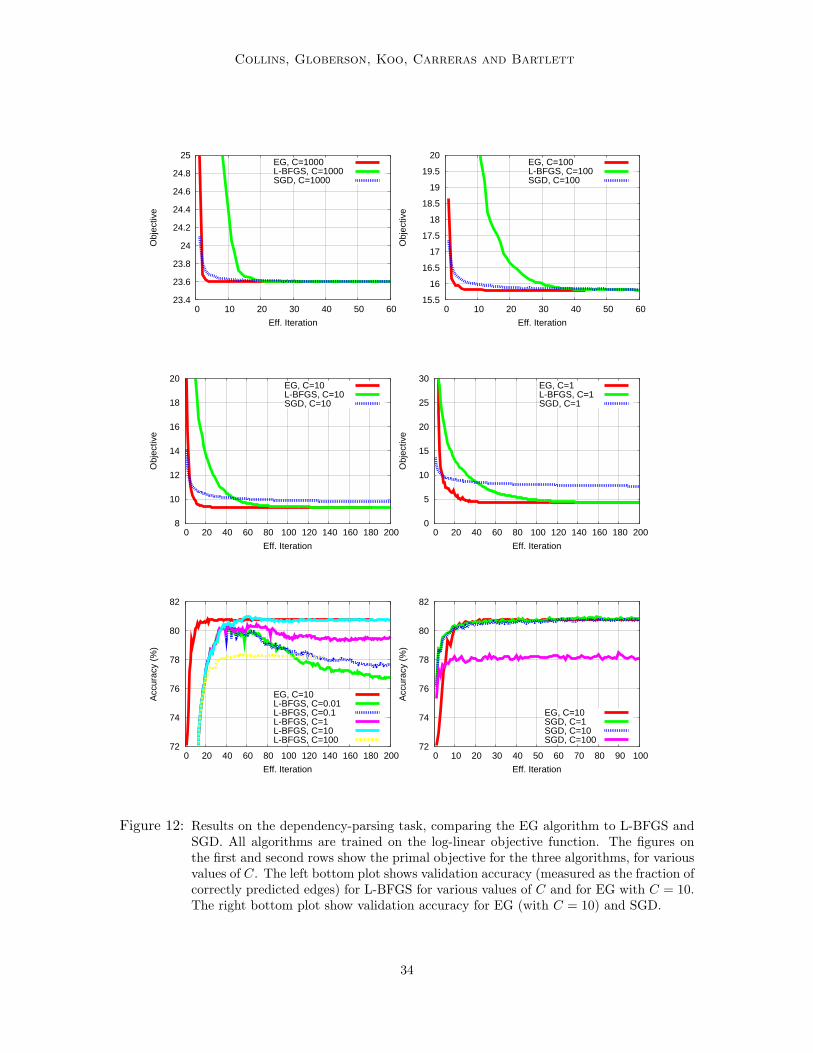
Collins, Globerson, Koo, Carreras and Bartlett
23.4
23.6
23.8
24
24.2
24.4
24.6
24.8
25
0 10 20 30 40 50 60
Obj
ectiv
e
Eff. Iteration
EG, C=1000L-BFGS, C=1000SGD, C=1000
15.5
16
16.5
17
17.5
18
18.5
19
19.5
20
0 10 20 30 40 50 60
Obj
ectiv
e
Eff. Iteration
EG, C=100L-BFGS, C=100SGD, C=100
8
10
12
14
16
18
20
0 20 40 60 80 100 120 140 160 180 200
Obj
ectiv
e
Eff. Iteration
EG, C=10L-BFGS, C=10SGD, C=10
0
5
10
15
20
25
30
0 20 40 60 80 100 120 140 160 180 200
Obj
ectiv
e
Eff. Iteration
EG, C=1L-BFGS, C=1SGD, C=1
72
74
76
78
80
82
0 20 40 60 80 100 120 140 160 180 200
Acc
urac
y (%
)
Eff. Iteration
EG, C=10L-BFGS, C=0.01L-BFGS, C=0.1L-BFGS, C=1L-BFGS, C=10L-BFGS, C=100
72
74
76
78
80
82
0 10 20 30 40 50 60 70 80 90 100
Acc
urac
y (%
)
Eff. Iteration
EG, C=10SGD, C=1SGD, C=10SGD, C=100
Figure 12: Results on the dependency-parsing task, comparing the EG algorithm to L-BFGS andSGD. All algorithms are trained on the log-linear objective function. The figures onthe first and second rows show the primal objective for the three algorithms, for variousvalues of C. The left bottom plot shows validation accuracy (measured as the fraction ofcorrectly predicted edges) for L-BFGS for various values of C and for EG with C = 10.The right bottom plot show validation accuracy for EG (with C = 10) and SGD.
34

Exponentiated Gradient Algorithms for CRFs and Max-Margin Markov Networks
8. Experiments on Max-Margin Models
The max-margin loss (Eq. 5) has a discontinuity in its derivative. This makes optimization ofmax-margin models somewhat more involved than log-linear ones, since gradient algorithmssuch as L-BFGS cannot be used. This difficulty is exacerbated in the case of structuredprediction models, since maximization in Eq. 5 is potentially over an exponentially largeset.
In this section, we apply the EG algorithm to the max-margin problem, and compare itsperformance to the SVM-Struct algorithm presented in Tsochantaridis et al. (2004).15 SVM-Struct is based on a cutting-plane algorithm that operates on the dual max-margin problem(D-MM) and results in monotone improvement in this dual. In this sense, it is similar toour EG algorithm. In order to facilitate a fair comparison, we report the performance ofthe two algorithms as a function of time. We do not report results by iteration since EGand SVM-struct involve different computation per iteration (e.g., SVM-Struct solves a QPper iteration).
We applied SVM-Struct and EG to the dependency parsing problem described in Sec-tion 7.2. To apply SVM-Struct to this problem, we supply it with a routine that findsthe y ∈ Y which attains the maximum of the hinge-loss in Eq. 5. This maximum canbe found using a Viterbi-style algorithm. For the value of C we experimented with C ∈{1, 10, 100, 1000, 10000}. The optimal value in terms of validation error was C = 100.
Figure 13 shows results in terms of primal and dual objective and in terms of accuracy.It can be seen that EG is considerably faster than SVM-Struct for most C values. Theperformance is comparable only for C = 1, where convergence is slow for both algorithms.
9. Conclusion
We have presented novel algorithms for large-scale learning of log-linear and max-marginmodels, which provably converge to the optimal value of the respective loss functions. Al-though the algorithms have both batch and online variants, the online version turns out tobe much more effective, both in theory and in practice. Our theoretical results (see Sec-tion 5.1) suggest that the online algorithm requires a factor of n less iterations to achievea desired accuracy ε in the dual objective. This factor results from the fact that the onlinealgorithm can use a learning rate η that is n times larger than the batch case to obtainupdates that decrease the dual objective. Intuitively, this difference is associated with thefact that the batch algorithm updates all α values simultaneously. The dual objective hasa term αTAα which involves all the αi variables and second order interactions betweenthem. It turns out that for batch updates only a relatively small change in the αi is al-lowed, if one still requires an improvement in the dual objective after the update. It ispossible that our bounds for the batch convergence rate are more conservative than thosefor the online case. However, we have observed in practice that the batch algorithm is muchslower to converge. Furthermore, we also observed that other batch-based algorithms suchas L-BFGS and conjugate gradient converge more slowly than the online EG algorithm.
Our results provide an O(log(1ε )) rate for the log-linear model, as opposed to O(1
ε ) formax-margin. If these bounds are tight, they would imply that log-linear models have an
15. Code available from svmlight.joachims.org/svm struct.html
35

Collins, Globerson, Koo, Carreras and Bartlett
0
5
10
15
20
25
30
35
40
45
0 1 2 3 4 5 6 7 8 9 10
Obj
ectiv
e
CPU Time (hours)
EG Primal, C=1000EG Dual, C=1000SVM-S Primal, C=1000SVM-S Dual, C=1000
0
5
10
15
20
25
30
35
40
45
0 5 10 15 20 25
Obj
ectiv
e
CPU Time (hours)
EG Primal, C=100EG Dual, C=100SVM-S Primal, C=100SVM-S Dual, C=100
0
5
10
15
20
25
0 5 10 15 20 25 30
Obj
ectiv
e
CPU Time (hours)
EG Primal, C=10EG Dual, C=10
SVM-S Primal, C=10SVM-S Dual, C=10
0
5
10
15
20
25
0 5 10 15 20 25 30
Obj
ectiv
e
CPU Time (hours)
EG Primal, C=1EG Dual, C=1SVM-S Primal, C=1SVM-S Dual, C=1
74
75
76
77
78
79
80
81
82
0 5 10 15 20 25 30
Acc
urac
y (%
)
CPU Time (hours)
EG, C=100SVM-S, C=100SVM-S, C=10
Figure 13: Results on the dependency-parsing task, comparing the EG algorithm to SVM-Struct.Both algorithms are trained on a max-margin model. The figures on the first and secondrows show the primal objective for both algorithms, for various values of C. The bottomcurve shows validation accuracy (measured as the fraction of correctly predicted edges)for SVM-Struct for various values of C and for EG with C = 100 (the value that yieldedthe highest validation accuracy). The X axis on all curves is running time in hours.
36

Exponentiated Gradient Algorithms for CRFs and Max-Margin Markov Networks
advantage over max-margin ones in terms of training efficiency. However, it is possible thatthe analysis is not tight, and that improved rates may also be obtained for the max-marginmodel. In any case, this raises the interesting question of comparing classification modelsnot only in terms of accuracy but also in terms of optimization efficiency.
Our convergence rates are with respect to accuracy in the dual objective. Some previouswork (e.g. Shalev-Shwartz et al., 2007) has considered the accuracy with respect to theprimal objective. It is relatively easy to show that in our case this still results in anO(log(1
ε )) for the log-linear problem but a slower rate of O( 1ε2
) for the max-margin case. Itis possible that more refined analysis will result in O(1
ε ), but we leave this for further study.Most of our proofs rely on a relation between BQ and the KL divergence. This relation
holds for max-margin learning as well, a fact that simplifies previous results in this setting(Bartlett et al., 2005). We expect a similar analysis to hold for other functions Q.
An interesting extension of our method is to using second order derivative information,or its approximations, as in L-BFGS (Byrd et al., 1995). Such information may be used toobtain more accurate minimization for each αi and may speed up convergence. Anotherpossible improvement is to the line search method. In the experiments reported here weuse a crude mechanism for adapting the learning rate, and it is possible that a more carefulprocedure will improve convergence rates in practice.
Finally, our results show that the EG algorithms are highly competitive with state-of-the-art methods for training log-linear and max-margin models. We thus expect them tobecome useful as learning algorithms, specifically in the structured prediction setting, wheresome of the standard multi-class algorithms are not applicable.
Acknowledgments
The authors gratefully acknowledge the following sources of support. Amir Globerson wassupported by a fellowship from the Rothschild Foundation - Yad Hanadiv. Terry Koo wasfunded by a grant from the NSF (DMS-0434222) and a grant from NTT, Agmt. Dtd.6/21/1998. Xavier Carreras was supported by the Catalan Ministry of Innovation, Univer-sities and Enterprise, and by a grant from NTT, Agmt. Dtd. 6/21/1998. Michael Collinswas funded by NSF grants 0347631 and DMS-0434222. Peter Bartlett was funded by agrant from the NSF (DMS-0434383).
References
J. Baker. Trainable grammars for speech recognition. In J.J. Wolf and D.H. Klatt, editors,97th meeting of the Acoustical Society of America, pages 547–550. Acoust. Soc. Am., NewYork, NY, 1979.
P. L. Bartlett, M. Collins, B. Taskar, and D. McAllester. Exponentiated gradient algorithmsfor large–margin structured classification. In L. K. Saul, Y. Weiss, and L. Bottou, editors,Advances in Neural Information Processing Systems 17, pages 113–120, Cambridge, MA,2005. MIT Press.
A. Beck and M. Teboulle. Mirror descent and nonlinear projected subgradient methods forconvex optimization. Operations Research Letters, 31:167–175, 2003.
37

Collins, Globerson, Koo, Carreras and Bartlett
L.M. Bregman. The relaxation method of finding the common point of convex sets and itsapplication to the solution of problems in convex programming. U.S.S.R. ComputationalMathematics and Mathematical Physics, 7:200–217, 1967.
S. Buchholz and E. Marsi. CoNLL-X shared task on multilingual dependency parsing.In Proceedings of the Tenth Conference on Computational Natural Language Learning(CoNLL-X), pages 149–164, 2006.
R.H. Byrd, P. Lu, and J. Nocedal. A limited memory algorithm for bound constrainedoptimization. SIAM Journal on Scientific and Statistical Computing, 16(5):1190–1208,1995.
Y. Censor and S.A. Zenios. Parallel optimization. Oxford University Press, 1997.
M. Civit and M. Antonia Martı. Design principles for a Spanish treebank. In Proceedingsof the First Workshop on Treebanks and Linguistic Theories (TLT), 2002.
T.M. Cover and J.A Thomas. Elements of Information Theory. Wiley, 1991.
K. Crammer and Y. Singer. On the algorithmic implementation of multiclass kernel-basedvector machines. Journal of Machine Learning Research, 2:265–292, 2002.
N. Cristianini, C. Campbell, and J. Shawe-Taylor. Multiplicative updatings for support-vector learning. Technical report, NeuroCOLT2,, 1998.
A. Globerson, T. Koo, , X. Carreras, and M. Collins. Exponentiated gradient algorithmsfor log-linear structured prediction. In Proceedings of the Twenty-Fourth InternationalConference on Machine Learning. ACM, New York, NY, 2007.
D. Hush, P. Kelly, C. Scovel, and I. Steinwart. QP algorithms with guaranteed accuracyand run time for support vector machines. Journal of Machine Learning Research, 7:733–769, 2006.
T. Jaakkola and D. Haussler. Probabilistic kernel regression models. In Proceedings ofSeventh Workshop on Artificial Intelligence and Statistics. 1999.
T. Joachims. Training linear SVMs in linear time. In KDD ’06: Proceedings of the 12thACM SIGKDD international conference on Knowledge discovery and data mining, pages217–226. ACM Press, New York, NY, 2006.
S.S. Keerthi, K.B. Duan, S.K. Shevade, and A. N. Poo. A fast dual algorithm for kernellogistic regression. Machine Learning, 61:151–165, 2005.
J. Kivinen and M. Warmuth. Exponentiated gradient versus gradient descent for linearpredictors. Information and Computation, 132(1):1–63, 1997.
J. Kivinen and M. Warmuth. Relative loss bounds for multidimensional regression problems.Machine Learning, 45(3):301–329, 2001.
K. Koh, S.J. Kim, and S. Boyd. An interior point method for large scale l1-regularizedlogistic regression. Journal of Machine Learning Research, 8:1519–1555, 2007.
38

Exponentiated Gradient Algorithms for CRFs and Max-Margin Markov Networks
T. Koo, A. Globerson, X. Carreras, and M. Collins. Structured prediction models via thematrix-tree theorem. In Proceedings of the Conference on Empirical Methods in NaturalLanguage Processing (EMNLP). 2007.
J. Lafferty, A. McCallum, and F. Pereira. Conditonal random fields: Probabilistic modelsfor segmenting and labeling sequence data. In C.E. Brodley and A.P. Danyluk, editors,Proceedings of the Eighteenth International Conference on Machine Learning, pages 282–289, San Francisco, CA, 2001. Morgan Kaufmann.
G. Lebanon and J. Lafferty. Boosting and maximum likelihood for exponential models. InT.G. Dietterich, S. Becker, and Z. Ghahramani, editors, Advances in Neural InformationProcessing Systems 14, pages 447–454. MIT Press, Cambridge, MA, 2002.
Y. LeCun, L. Bottou, Y. Y. Bengio, and P. Haffner. Gradient-based learning applied todocument recognition. Proceedings of the IEEE, 86(11):2278–2324, November 1998.
R. McDonald, K. Crammer, and F. Pereira. Online large-margin training of dependencyparsers. In Proceedings of the 43rd Annual Meeting of the ACL, pages 91–98. Associationfor Computational Linguistics, Morristown, NJ, 2005.
R. Memisevic. Dual optimization of conditional probability models. Technical report, Univ.of Toronto, 2006.
T. Minka. A comparison of numerical optimizers for logistic regression. Technical report,CMU, 2003.
M. Mitzenmacher and E. Upfal. Probability and Computing: Randomized Algorithms andProbabilistic Analysis. Cambridge University Press, 2005.
J. Platt. Fast training of support vector machines using sequential minimal optimization.In Advances in Kernel Methods - Support Vector Learning. MIT Press, 1998.
F. Sha, Y. Lin, L.K. Saul, and D.D. Lee. Multiplicative updates for nonnegative quadraticprogramming. Neural Computation, 19(8):2004–2031, 2007.
F. Sha and F. Pereira. Shallow parsing with conditional random fields. In NAACL ’03:Proceedings of the 2003 Conference of the North American Chapter of the Association forComputational Linguistics on Human Language Technology, pages 134–141, Morristown,NJ, USA, 2003. Association for Computational Linguistics.
S. Shalev-Shwartz, Y. Singer, and N. Srebro. Pegasos: Primal estimated sub-gradient solverfor SVM. In Proceedings of the Twenty-Fourth International Conference on MachineLearning. ACM, New York, NY, 2007.
B. Taskar, C. Guestrin, and D. Koller. Max margin markov networks. In S. Thrun, L. Saul,and B. Scholkopf, editors, Advances in Neural Information Processing Systems 16. MITPress, Cambridge, MA, 2004a.
B. Taskar, D. Klein, M. Collins, D. Koller, and C. Manning. Max-margin parsing. InProceedings of the Conference on Empirical Methods in Natural Language Processing(EMNLP). 2004b.
39

Collins, Globerson, Koo, Carreras and Bartlett
C.H. Teo, Q. Le, A. Smola, and S.V.N. Vishwanathan. A scalable modular convex solverfor regularized risk minimization. In KDD ’07: Proceedings of the 13th ACM SIGKDDinternational conference on Knowledge discovery and data mining, pages 727–736. ACMPress, New York, NY, USA, 2007.
I. Tsochantaridis, T. Hofmann, T. Joachims, and Y. Altun. Support vector machine learningfor interdependent and structured output spaces. In C.E. Brodley, editor, Proceedings ofthe Twenty-First International Conference on Machine Learning. ACM, New York, NY,2004.
S.V. N. Vishwanathan, N. N. Schraudolph, M. W. Schmidt, and K. P. Murphy. Acceleratedtraining of conditional random fields with stochastic gradient methods. In W.W. Cohenand A. Moore, editors, Proceedings of the Twenty-Third International Conference onMachine Learning, pages 969–976. ACM Press, New York, NY, 2006.
T. Zhang. On the dual formulation of regularized linear systems with convex risks. MachineLearning, 46:91–129, 2002.
J. Zhu and T. Hastie. Kernel logistic regression and the import vector machine. In T.G.Dietterich, S. Becker, and Z. Ghahramani, editors, Advances in Neural Information Pro-cessing Systems 14, pages 1081–1088. MIT Press, Cambridge, MA, 2001.
40

Exponentiated Gradient Algorithms for CRFs and Max-Margin Markov Networks
Appendix A. O(1ε) Rate for Batch Algorithms - Proof of Lemma 5
We use a similar proof technique to that of Kivinen and Warmuth (2001). In particular, weneed the following Lemma, which is very similar to results used by Kivinen and Warmuth(2001):
Lemma 10 (See Kivinen and Warmuth (2001), Proof of Lemma 4) For any convex func-tion Q(α) over ∆n, for any u ∈ ∆n, and any αt in the interior of ∆n, if αt+1 is derivedfrom αt using the EG updates with a learning rate η, then
ηQ(αt)− ηQ(u) = D[u‖αt]−D[u‖αt+1] +D[αt‖αt+1]− ηBQ[u‖αt] (30)
Proof: By the definition of Bregman divergence, we have
ηQ(αt)− ηQ(u) = −η∇Q(αt) · (u−αt)− ηBQ[u‖αt] (31)
Given that αt+1 is derived from αt using EG updates,
αt+1i,y =
αti,ye−η∇i,y
Zti
where Zti is a normalization constant, and ∇i,y = ∂Q(αt)∂αi,y
. Simple algebra then shows thatif αt+1 is derived from αt using EG updates, then
D[u‖αt]−D[u‖αt+1] +D[αt‖αt+1] =∑i,y
(ui,y log
ui,yαti,y− ui,y log
ui,y
αt+1i,y
+ αti,y logαti,y
αt+1i,y
)
=∑i,y
(ui,y − αti,y) logαt+1i,y
αti,y
=∑i,y
(ui,y − αti,y)(−η∇i,y − logZti )
=∑i,y
(ui,y − αti,y)(−η∇i,y)
= −η∇Q(αt) · (u−αt) (32)
Note that we have used∑
i,y(ui,y−αti,y) logZti = 0, which follows because∑
i,y ui,y logZti =∑i,y α
ti,y logZti =
∑i logZti .
Combining Eq. 31 and Eq. 32 gives Eq. 30, thus proving the Lemma.We can now prove Lemma 5:Proof of Lemma 5: Using −ηBQ[u‖αt] ≤ 0, Lemma 10 implies that for all t
ηQ(αt)− ηQ(u) ≤ D[u‖αt]−D[u‖αt+1] +D[αt‖αt+1] (33)
By the assumptions of Lemma 5, Q(α) is τ -upper-bounded, and 0 ≤ η ≤ 1τ , hence by
Lemma 3 we haveQ(αt)−Q(αt+1) ≥ 1
ηD[αt‖αt+1] (34)
41

Collins, Globerson, Koo, Carreras and Bartlett
Combining Eqs. 33 and 34 gives for all t
ηQ(αt+1)− ηQ(u) ≤ D[u‖αt]−D[u‖αt+1]
Summing this over t = 1, . . . , T gives (the sum on the RHS telescopes)
η
T∑t=1
Q(αt+1)− ηTQ(u) ≤ D[u‖α1]−D[u‖αT+1]
Because Q(αt) is monotone decreasing (by Eq. 34), we have TQ(αT+1) ≤∑T
t=1Q(αt+1)and simple algebra gives
Q(αT+1) ≤ Q(u) +D[u‖α1]−D[u‖αT+1]
ηT
Dropping the term D[u‖αT+1] (because −D[u‖αT+1] ≤ 0) we obtain
Q(αT+1) ≤ Q(u) +D[u‖α1]ηT
as required.
Appendix B. O(log 1ε) Rate for Batch Algorithms - Proof of Lemma 6
By the assumptions of Lemma 6, Q(α) is τ -upper-bounded, and 0 ≤ η ≤ 1τ , hence by
Lemma 3 we have for all t
Q(αt)−Q(αt+1) ≥ 1ηD[αt‖αt+1] (35)
Combining this result with Lemma 10 gives
ηQ(αt+1)− ηQ(u) ≤ D[u‖αt]−D[u‖αt+1]− ηBQ[u‖αt]
We can now make use of the assumption thatQ(α) is (µ, τ)-bounded, and hence ηBQ[u‖αt] ≥µηD[u‖αt], to obtain
ηQ(αt+1)− ηQ(u) ≤ D[u‖αt]−D[u‖αt+1]− ηµD[u‖αt]= (1− ηµ)D[u‖αt]−D[u‖αt+1]≤ (1− ηµ)D[u‖αt] (36)
If for any t, Q(αt+1) − Q(u) ≤ 0 then because Q(αt) decreases monotonically with t wehave Q(αT+1) ≤ Q(αt+1) ≤ Q(u) and the Lemma holds. Otherwise, if Q(αt+1)−Q(u) ≥ 0for all t then for all t
D[u‖αt+1] ≤ (1− ηµ)D[u‖αt] . (37)
Using this inequality recursively for t = 1, . . . , T we get
D[u‖αT+1] ≤ (1− ηµ)T D[u‖α1] (38)
Substituting back into Eq. 36 we obtain
Q(αt+1)−Q(u) ≤ (1− ηµ)T
ηD[u‖α1] ≤ e−ηµT
ηD[u‖α1] (39)
where we have used log(1− x) ≤ −x.
42
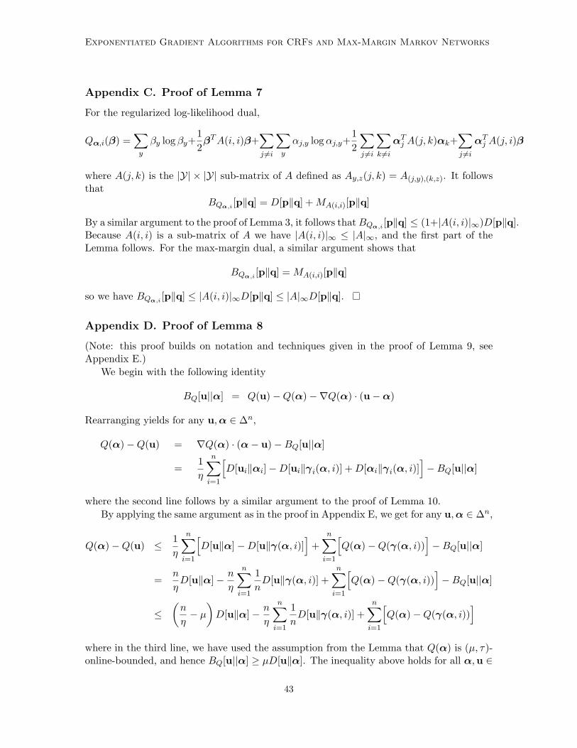
Exponentiated Gradient Algorithms for CRFs and Max-Margin Markov Networks
Appendix C. Proof of Lemma 7
For the regularized log-likelihood dual,
Qα,i(β) =∑y
βy log βy+12βTA(i, i)β+
∑j 6=i
∑y
αj,y logαj,y+12
∑j 6=i
∑k 6=i
αTj A(j, k)αk+∑j 6=iαTj A(j, i)β
where A(j, k) is the |Y| × |Y| sub-matrix of A defined as Ay,z(j, k) = A(j,y),(k,z). It followsthat
BQα,i [p‖q] = D[p‖q] +MA(i,i)[p‖q]
By a similar argument to the proof of Lemma 3, it follows thatBQα,i [p‖q] ≤ (1+|A(i, i)|∞)D[p‖q].Because A(i, i) is a sub-matrix of A we have |A(i, i)|∞ ≤ |A|∞, and the first part of theLemma follows. For the max-margin dual, a similar argument shows that
BQα,i [p‖q] = MA(i,i)[p‖q]
so we have BQα,i [p‖q] ≤ |A(i, i)|∞D[p‖q] ≤ |A|∞D[p‖q].
Appendix D. Proof of Lemma 8
(Note: this proof builds on notation and techniques given in the proof of Lemma 9, seeAppendix E.)
We begin with the following identity
BQ[u||α] = Q(u)−Q(α)−∇Q(α) · (u−α)
Rearranging yields for any u,α ∈ ∆n,
Q(α)−Q(u) = ∇Q(α) · (α− u)−BQ[u||α]
=1η
n∑i=1
[D[ui‖αi]−D[ui‖γi(α, i)] +D[αi‖γi(α, i)]
]−BQ[u||α]
where the second line follows by a similar argument to the proof of Lemma 10.By applying the same argument as in the proof in Appendix E, we get for any u,α ∈ ∆n,
Q(α)−Q(u) ≤ 1η
n∑i=1
[D[u‖α]−D[u‖γ(α, i)]
]+
n∑i=1
[Q(α)−Q(γ(α, i))
]−BQ[u||α]
=n
ηD[u‖α]− n
η
n∑i=1
1nD[u‖γ(α, i)] +
n∑i=1
[Q(α)−Q(γ(α, i))
]−BQ[u||α]
≤(n
η− µ
)D[u‖α]− n
η
n∑i=1
1nD[u‖γ(α, i)] +
n∑i=1
[Q(α)−Q(γ(α, i))
]where in the third line, we have used the assumption from the Lemma that Q(α) is (µ, τ)-online-bounded, and hence BQ[u||α] ≥ µD[u‖α]. The inequality above holds for all α,u ∈
43

Collins, Globerson, Koo, Carreras and Bartlett
∆n, so we can take α = α(kt−11 ) for any sequence kt−1
1 . Taking expectations of both sides,and using similar arguments to those in Appendix E, we get
ET
[Q(α(kt−1
1 ))]−Q(u) ≤
(n
η− µ
)ET
[D[u‖α(kt−1
1 )]]− n
ηET
[D[u‖α(kt1)]
]+ nET
[Q(α(kt−1
1 ))]− nET
[Q(α(kt1))
](40)
where ET is again an expectation with respect to the sequence kT1 being drawn from theuniform distribution over [1 . . . n]T . For convenience, define
Qt ≡ ET
[Q(α(kt1))
]−Q(u) and Dt ≡ 1
ηET
[D[u||α(kt1)]
]Then, Eq. 40 can be rearranged to give
Qt−1 ≤ (n− ηµ)Dt−1 − nDt + nQt−1 − nQt
nQt + nDt ≤ (n− 1)Qt−1 + (n− ηµ)Dt−1 ≤ (n− ηµ)(Qt−1 + Dt−1
)(41)
Qt + Dt ≤(
1− ηµ
n
)(Qt−1 + Dt−1
)where Eq. 41 uses the observation that n− ηµ ≥ n− 1 because ηµ ≤ 1 (this follows becauseη ≤ 1/τ and µ < τ for some τ > 0). By iterating this result, it follows that
QT + DT ≤(
1− ηµ
n
)T (Q0 + D0
)ET
[Q(α(kT1 ))
]≤ Q(u) +
(1− ηµ
n
)T (Q(α1)−Q(u) +
1ηD[u||α1]
)≤ Q(u) + e−ηµT/n
(Q(α1)−Q(u) +
1ηD[u||α1]
)(42)
thus proving the Lemma.
Appendix E. Proof of Lemma 9
For the proof we will need some additional notation, which makes explicit the relation-ship between the sequence of dual variables α1,α2, . . . ,αT+1 and the sequence of indicesk1, k2, . . . , kT used in the algorithm in Figure 2. We will use the following definitions:
• We use kt1 to denote a sequence of indices k1, k2, . . . , kt. We take k01 to be the empty
sequence.
• We write γ : ∆n × [1 . . . n] → ∆n to denote the function that corresponds to an EGupdate on a single example. More specifically, if β = γ(α, k) then we have
βi = αi for i 6= k
βi,y ∝ αi,y exp{−η∇i,y} where ∇i,y = ∂Q(α)∂αi,y
for i = k, for all y.
44

Exponentiated Gradient Algorithms for CRFs and Max-Margin Markov Networks
• Finally, for any choice of index sequence kT1 we will define a sequence of dual variablesusing the following iterative definition:
α(k01) = α1
α(kt1) = γ(α(kt−11 ), kt) for t ≥ 1.
Here α1 is the initial setting of the dual variables, as shown in the algorithm in figure 2.
From these definitions it follows that if kT1 is the sequence of indices chosen during a runof the algorithm in figure 2, then the sequence of dual variables α1,α2, . . . ,αT+1 is suchthat αt+1 = α(kt1) for t = 0 . . . T . We can now give the proof.
Proof of Lemma 9. First, we have for any α,u ∈ ∆n
Q(α) ≤ Q(u) + (α− u) · ∇Q(α)
= Q(u) +1η
n∑i=1
D[ui‖αi]−D[ui‖γi(α, i)] +D[αi‖γi(α, i)] (43)
The second line again follows by similar arguments to those in the proof of Lemma 10.Next consider the terms on the right-hand-side of the inequality. For any i, we have
D[ui‖αi]−D[ui‖γi(α, i)]= D[ui‖αi]−D[ui‖γi(α, i)] +
∑j=1...n,j 6=i
D[uj‖αj ]−∑
j=1...n,j 6=iD[uj‖αj ] (44)
= D[ui‖αi]−D[ui‖γi(α, i)] +∑
j=1...n,j 6=iD[uj‖αj ]−
∑j=1...n,j 6=i
D[uj‖γj(α, i)] (45)
= D[u‖α]−D[u‖γ(α, i)] (46)
Here Eq. 45 follows from Eq. 44 because γj(α, i) = αj for j 6= i.In addition, for any i we have
1ηD[αi‖γi(α, i)] ≤ Q(α)−Q(γ(α, i)) (47)
This follows because by the assumption in the Lemma, Q(α) is τ -online-upper-bounded, sowe have BQα,i [γi(α, i)‖αi] ≤ τD[γi(α, i)‖αi]. By an application of Lemma 2 to the convexfunction Qα,i, noting that by assumption η ≤ 1/τ , it follows that
1ηD[αi‖γi(α, i)] ≤ Qα,i(αi)−Qα,i(γi(α, i))
Finally, note that Qα,i(αi) = Q(α), and Qα,i(γi(α, i)) = Q(γ(α, i)), giving the result inEq. 47.
Combining Equations 43, 46 and 47 gives for any α,
Q(α) ≤ Q(u) +1η
n∑i=1
[D[u‖α]−D[u‖γ(α, i)]] +n∑i=1
[Q(α)−Q(γ(α, i))] (48)
45

Collins, Globerson, Koo, Carreras and Bartlett
Because Eq. 48 holds for any value of α, we have for all t = 1 . . . T , for all kt−11 ∈ [1 . . . n]t−1,
Q(α(kt−11 )) ≤ Q(u) +
1η
n∑i=1
[D[u‖α(kt−1
1 )]−D[u‖γ(α(kt−11 ), i)]
]+
n∑i=1
[Q(α(kt−1
1 ))−Q(γ(α(kt−11 ), i))
](49)
We can now take an expectation of both sides of the inequality in Eq. 49. For any functionf(kt1), we use the notation Et[f(kt1)] to denote the expected value of f(kt1) when kt1 is drawnuniformly at random from [1, 2, . . . , n]t; more precisely
Et[f(kt1)] =1nt
∑kt1∈[1,2,...,n]t
f(kt1)
We apply the operator Et−1 to both sides of Eq. 49. We consider the different terms inturn. First,
Et−1[Q(α(kt−11 ))] = ET [Q(α(kt−1
1 ))]
This follows because Q(α(kt−11 )) does not depend on the values for kt, . . . , kT . Clearly,
Et−1[Q(u)] = Q(u). Next,
Et−1
[1η
n∑i=1
D[u‖α(kt−11 )]−D[u‖γ(α(kt−1
1 ), i)]
]
= Et−1
[n
ηD[u‖α(kt−1
1 )]]−Et−1
[n
η
n∑i=1
1nD[u‖γ(α(kt−1
1 ), i)]
]
= Et−1
[n
ηD[u‖α(kt−1
1 )]]−Et
[n
ηD[u‖α(kt1)]
]= ET
[n
ηD[u‖α(kt−1
1 )]]−ET
[n
ηD[u‖α(kt1)]
]Finally, we consider the last term:
Et−1
[n∑i=1
Q(α(kt−11 ))−Q(γ(α(kt−1
1 ), i))
]
= Et−1
[nQ(α(kt−1
1 ))− nn∑i=1
1nQ(γ(α(kt−1
1 ), i))
]= Et−1
[nQ(α(kt−1
1 ))]−Et
[nQ(α(kt1))
]= ET
[nQ(α(kt−1
1 ))]−ET
[nQ(α(kt1))
]Combining these results with Eq. 49 gives
ET [Q(α(kt−11 ))] ≤ Q(u) + ET
[n
ηD[u‖α(kt−1
1 )]]−ET
[n
ηD[u‖α(kt1)]
]+ET
[nQ(α(kt−1
1 ))]−ET
[nQ(α(kt1))
](50)
46

Exponentiated Gradient Algorithms for CRFs and Max-Margin Markov Networks
Summing Eq. 50 over t = 1 . . . T gives
T∑t=1
ET [Q(α(kt−11 ))] ≤ TQ(u) + ET
[n
ηD[u‖α(k0
1)]]−ET
[n
ηD[u‖α(kT1 )]
]+ET
[nQ(α(k0
1))]−ET
[nQ(α(kT1 ))
]≤ TQ(u) +
n
ηD[u‖α(k0
1)] + n[Q(α(k0
1))−Q(α∗)]
= TQ(u) +n
ηD[u‖α1] + n
[Q(α1)−Q(α∗)
](51)
where α∗ = argminα∈∆n Q(α). Finally, note that for any value of kT1 we have Q(α(kt1)) ≤Q(α(kt−1
1 )) for t = 1 . . . T . Thus
ET [Q(α(kt1))] ≤ ET [Q(α(kt−11 ))]
and
TET [Q(α(kT1 )] ≤T∑t=1
ET [Q(α(kt−11 ))]
Combining this with Eq. 51 gives
TET [Q(α(kT1 )] ≤ TQ(u) +n
ηD[u‖α1] + n
[Q(α1)−Q(α∗)
]thus proving the lemma.
47