export failure and its consequences - jesse...
TRANSCRIPT

Export Failure and Its Consequences:Evidence from Colombian Exporters
Jesse Mora
UC Santa Cruz
November 6, 2014

Introduction
I. Exporting has a lot of benefits and yet few firms export (Bernardand Jensen, 2004; Brooks, 2006)
II. Fixed export costs play a particularly important role in limitinginternational trade
⇒ Estimates: around half a million US dollars for a single firm in LatinAmerica (Das, Roberts, and Tybout, 2007; Morales, Sheu, andZahler, 2011)
III. Fixed export costs may exceed export revenue
⇒ First time exporters tend to start small (Rauch and Watson, 2003)
1 / 39

Introduction
I. The majority of firms are unable to export beyond one year(Eaton, Eslava, Kugler, and Tybout, 2007)
⇒ Exporting likely resulted in profit losses
II. Trade literature treats exporting as a harmless exercise andlargely ignores export failure
III. What if exporting is not a harmless exercise?
2 / 39

Firms After They Try to Export and Fail
I. Firms rely on external financing for exporting (Amiti andWeinstein, 2011)
II. For some firms, export profit losses may result in lower financing
⇒ limit hiring, marketing, capital investments, etc.
III. So export costs are uncertain and the costs of export failure—notjust the probability of export failure—result in
⇒ lowers expected returns from exporting
⇒ fewer firms exporting
3 / 39

Example: InterSoftware/Air-Go Tech. (Mexico)
I. Established in 1996
II. Exported to the U.S. in 2001
III. Went bankrupt in 2002
IV. Hector Obregon, Chief Executive Officer, in Software Guru (2008)
⇒ “The most serious issue was that the expansions distracted us frompaying attention to issues with our principal business”
⇒ “Short-term cash flow became an issue and our credit lines werequickly saturated”
4 / 39

Paper Contributions
I. Partial Equilibrium Model: Failed export attempts paired withfinancial frictions can have a negative feedback effect
⇒ For lower productivity firms, export failure tightens the financialconstraint, decreases domestic sales, or even results in default
II. Stylized Facts: Export failure is associated with reduceddomestic-market performance for financially constrained firms
1) Higher probability of going out of business
2) For surviving firms, decrease in domestic revenue and
3) lower domestic revenue growth
III. Empirics: Quantify the consequences of export failure
⇒ Identification: Difference-in-difference, PSM, and IV estimatesusing Colombian firm-level data
5 / 39

Does Export Failure Result in Domestic-Market Exit?
Figure 1: Firm Entry and Exit
Note: The Figure shows the average share of firms in the data bycohort and firm type at time t . By design, the number of firms in thedata do not change at t = −2,−1, 0. Figure for Matched Data
6 / 39

What We Know
I. Financial frictions matter
⇒ Can affect which firms export and how much they export (Manova,2013)
⇒ Exporters are more likely to face liquidity constraints (Chaney, 2013)
⇒ Exporters are more risky because they have higher rates of defaultrates, conditional on exit (Antunes, Opromolla, and Russ, 2014)
II. Developing countries are different
⇒ Export survival is lower in developing countries (Besedes andPrusa, 2011, 2006a & 2006b)
⇒ ”Underdeveloped countries often have underdeveloped financialmarkets” (Moll, 2014)
7 / 39

What We Know
I. Financial frictions matter
⇒ Can affect which firms export and how much they export (Manova,2013)
⇒ Exporters are more likely to face liquidity constraints (Chaney, 2013)
⇒ Exporters are more risky because they have higher rates of defaultrates, conditional on exit (Antunes et al., 2014)
II. Developing countries are different
⇒ Export survival is lower in developing countries (Besedes andPrusa, 2011, 2006a & 2006b)
⇒ ”Underdeveloped countries often have underdeveloped financialmarkets” (Moll, 2014)
7 / 39
What We Know
I. There are trade offs between the home and foreign market
⇒ There is an immediate opportunity costs to exporting
– See Ahn and McQuoid (2013); McQuoid and Rubini (2014); Rho andRodrigue (2010)
⇒ Other trade offs result from various firm decisions:
– investment (Spearot, 2013)
– pricing (Soderbery, 2014)
– entry and exit (Blum, Claro, and Horstmann, 2013)
8 / 39

I. A Model with Export Failure, Marketing Costs, andFinancial Frictions

A Melitz-Type Model with Export Failure
I. Financing need and financial frictions (Manova, 2013)
II. Firm must spend on marketing in each market (Arkolakis, 2010)
III. I add an element of uncertainty in export success:
⇒ Firms are randomly matched with foreign partners
⇒ Unsuccessful matches result in export failure
⇒ So similar productivity firms may differ in export success
9 / 39

Consumers Maximize Utility
I. Individual demand of variety i : ci = A · p−σi
⇒ Assumes CES preferences
⇒ pi is the price of variety i
⇒ A is a demand parameter
⇒ σ > 1 is the elasticity of substitution between two goods
II. Total demand: qi = Li · ci = Li · A · p−σi
⇒ Li is the number of consumers
⇒ Li is endogenously determined by a firm’s marketing expenditure
10 / 39
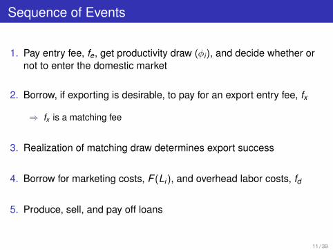
Sequence of Events
1. Pay entry fee, fe, get productivity draw (φi ), and decide whether ornot to enter the domestic market
2. Borrow, if exporting is desirable, to pay for an export entry fee, fx
⇒ fx is a matching fee
3. Realization of matching draw determines export success
4. Borrow for marketing costs, F (Li), and overhead labor costs, fd
5. Produce, sell, and pay off loans
11 / 39

All Firms: Ex Ante Maximization Problem
The maximization problem for potential exporter i :
Eπx (φi) = γEπsuccx (φi) + (1− γ)Eπfail
x (φi)
⇒ γ = the probability that a firm is successfully matched with aforeign partner
⇒ Export if Eπx (φi) > 0
Figure: The Ex Ante Export Entry Decision

Failed Exporter: Ex Post Maximization Problem
The Profit Function:
Eπ(φi) = maxpi ,qi ,Li
{piqi −
qi
φi− λBi − (1− λ)fe
}
Subject to:
Total Demand: qi = LiAp−σi
Marketing Expenditure: F (Li) = LβiThe Firm’s Liquidity Constraint: piqi − qi
φi≥ Bi
Creditors’ Constraint: λBi + (1− λ)fe ≥ fx + fd + F (Li)
13 / 39

Definitions
The Profit Function:
Eπ(φi) = maxpi ,qi ,Li
{piqi −
qi
φi− λBi − (1− λ)fe
}Where:Loan Repayment: Bi
Probability of Repayment: λ
Collateral/Entry Fee: feExport Fixed Costs/Matching Fee: fxOverhead Labor Costs: fd
Key Assumptions:Assumption 1) It is more expensive to export: fx > fd
Assumption 2) Default is not desirable: max{
fe−fdfe , 1
β
}< λ
14 / 39
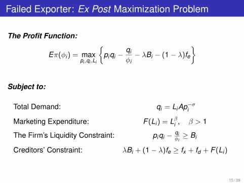
Failed Exporter: Ex Post Maximization Problem
The Profit Function:
Eπ(φi) = maxpi ,qi ,Li
{piqi −
qi
φi− λBi − (1− λ)fe
}
Subject to:
Total Demand: qi = LiAp−σi
Marketing Expenditure: F (Li) = Lβi , β > 1
The Firm’s Liquidity Constraint: piqi − qiφi≥ Bi
Creditors’ Constraint: λBi + (1− λ)fe ≥ fx + fd + F (Li)
15 / 39

Summary of Theoretical Propositions
For some failed exporters—relative to similar non-exporters andsuccessful exporters—entering a foreign market results in
I. firms becoming financially constrained,
II. financially constrained firms decreasing domestic sales,
⇒ Results from a decrease in borrowing for marketing
III. firms exiting the domestic marketDetails
16 / 39

With No Fin. Frictions or Exp. Failure (Melitz, 2003)
17 / 39
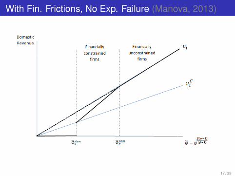
With Fin. Frictions, No Exp. Failure (Manova, 2013)
17 / 39

With Financial Frictions and Export Failure
17 / 39

II. Export failure is associated with reduceddomestic-market performance.
Colombian Firm-Level Data
I. Exports Data (1994–2011): Disaggregated data for all exporters
⇒ Source: Colombian Customs Agency (DIAN)
II. Domestic Data (1995–2011): Financial data for firms under thejurisdiction of the “Superintendencia de Sociedades”
⇒ Source: El sistema de Informacion y Reporte Empresarial(SIREM), reported by Superintendencia de Sociedades
Firm-type availability
18 / 39

Definitions: Outcome Variables
I. Firm Exitsi — Equals one if the firm exits the domestic marketand zero otherwise
II. Domestic Revenueit — Domestic revenue for firm i at time t
⇒ Subtract exports from revenue to calculate the domestic revenue
III. Ln(Domestic Revenueit ) — Log domestic revenue for firm i attime t
IV. Domestic Revenue Growthi — Difference in log domesticrevenue between time t and time t − 1
19 / 39
Definitions: Covariates
I. Successful Exportert — Equals one if the firm exports beyondone year and zero otherwise
⇒ Classification does not vary by firm
⇒ Includes firms going in and out of the export market
II. Not Financially Vulnerablei (NFVi ) — Equals one if the ratio ofcash flow from operations to total assets is greater than themedian at time of first exporting (t = 0) and zero otherwise
⇒ Classification does not vary by firm
⇒ A lower ratio implies a firm will have less cash available for futureperiods
⇒ The ratio is widely use in the literature (Ahn and McQuoid, 2013;Whited and Wu, 2006; Kaplan and Zingales, 1997).
20 / 39

Figure 2: Ln(Domestic Revenue): Unsuccessful Exporters(Constrained Firms)
Note: Regression includes firm fixed effects and year fixed effects.The periods are interacted with not financially constrained, non-exporters, and successful exporters. The omitted group is con-strained, unsuccessful exporters at time t = −1.
Poisson Levels21 / 39

Figure 3: Ln(Domestic Revenue): Unsuccessful vs. Successful Exporters(Constrained Firms)
Note: Regression includes firm fixed effects and year fixed effects.The periods are interacted with not financially constrained, non-exporters, and successful exporters. The omitted group is con-strained, unsuccessful exporters at time t = −1.
Poisson Levels22 / 39
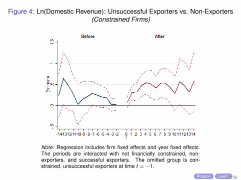
Figure 4: Ln(Domestic Revenue): Unsuccessful Exporters vs. Non-Exporters(Constrained Firms)
Note: Regression includes firm fixed effects and year fixed effects.The periods are interacted with not financially constrained, non-exporters, and successful exporters. The omitted group is con-strained, unsuccessful exporters at time t = −1.
Poisson Levels23 / 39

Figure 5: ∆Ln(Dom. Revenue) for Unsuccessful Exporters(Constrained Firms)
Note: Regression includes firm fixed effects and year fixed effects.The periods are interacted with not financially constrained, non-exporters, and successful exporters. The omitted group is con-strained, unsuccessful exporters at time t = −1.
24 / 39

Figure 6: ∆Ln(Dom. Revenue): Unsuccessful vs. Successful Exporters(Constrained Firms)
Note: Regression includes firm fixed effects and year fixed effects.The periods are interacted with not financially constrained, non-exporters, and successful exporters. The omitted group is con-strained, unsuccessful exporters at time t = −1.
25 / 39

Figure 7: ∆Ln(Dom. Revenue): Unsuccessful Exporters vs. Non-Exporters(Constrained Firms)
Note: Regression includes firm fixed effects and year fixed effects.The periods are interacted with not financially constrained, non-exporters, and successful exporters. The omitted group is con-strained, unsuccessful exporters at time t = −1.
26 / 39

III. The Consequences of Export Failure

Identification Strategy
I. Baseline estimates: Difference-in-difference with firm fixed effects
⇒ Outcome variables: log domestic revenue, ∆log domestic revenue,domestic revenue, and firm exits
II. PSM estimates: Match unsuccessful exporters to successful exporterand non-exporting firms
⇒ Matched based on pre-exporting variables: revenue, revenue growth, cashflow/total assets, short-term and long-term debt, short-term and long-termlabor, sort-term and long-term investment, inventory, property, andintangibles
III. IV estimates: Attempt to bring in external variation to addressendogeneity concerns
27 / 39

Estimation Model
Yit = αi + δt + β1Afterit + β2Afterit · Successfuli + uit
Where:
⇒ Yit is a measurement of success in the domestic market
⇒ αi are firm fixed effects
⇒ δt are year fixed effects
⇒ Afterit = 1 for all periods after first exporting and zero otherwise– In estimates: β1Afterit → β11After(t = 0)it + β12After(t = 1 to 5)it + β13After(rest)it
⇒ Successfuli = 1 for firms exporting more than one year and zerootherwise
– Since I use within firm variation, successful is not included in the model
– In estimates:
β2Afterit · Succi → β21After(t = 0)it · Succi + β22After(t = 1 to 5)it · Succi + β23After(rest)it · Succi
28 / 39

Table 1: Exporting Increases the Probability of Going Out of Business
Dependent= Exit All Survived SR Surv. SR & MR
Successful -0.32*** -0.26*** -0.02(0.03) (0.04) (0.02)
SuccessfulxNFV 0.09** 0.09* -0.03(0.05) (0.05) (0.03)
Not Fin. Vulnerable (NFV) -0.10*** -0.09** 0.02(0.04) (0.04) (0.02)
First Export Valuet=0 -0.00*** -0.00*** -0.00(0.00) (0.00) (0.00)
Avg. Short-Term Debtt<0 0.02** 0.02* 0.01(0.01) (0.01) (0.01)
Avg. Long-Term Debtt<0 0.02** 0.03** 0.01(0.01) (0.01) (0.01)
Avg. Long-Term Investmentt<0 -0.02* -0.02** -0.00(0.02) (0.02) (0.01)
Number of observations 1,240 1,192 1,013Adjusted R2 0.179 0.142 0.070
Note: *** p < 0.01, ** p < 0.05, * p < 0.1. Robust standard errors in parenthesis.The regressions also control for industry, export cohort, short-term labor, long-termlabor, inventory, property, short-term debt, domestic revenue, and intangibles.
29 / 39

Table 2: Baseline Estimates: All Data
Dependent → ∆Ln(Dom. Rev.) Ln(Dom. Rev.)
(1) (2) (3) (4)Base Base*NFV Base Base*NFV
Year of exp -0.16*** -0.07**(0.03) (0.03)
After (t=1 to 5) -0.19*** -0.32***(0.03) (0.05)
After (rest) -0.15*** -0.56***(0.04) (0.09)
Successful*(Year of exp) 0.05 0.17***(0.03) (0.04)
Successful*After(t=1 to 5) 0.04 0.35***(0.03) (0.06)
Successful*After(rest) -0.05 0.45***(0.03) (0.09)
Firm and year fixed effects Yes YesNumber of observations 15,381 16,161Number of clusters/groups 1,412 1,412Adjusted R2 0.042 0.252
Note: *** p < 0.01, ** p < 0.05, * p < 0.1; robust standard errors, clustered at the firmlevel, shown in parenthesis; and Not Financially Constrained(NFV) equals 1 if the firm hasa cash flow to total assets ratio greater than .07 (the median ratio for all firms).
30 / 39
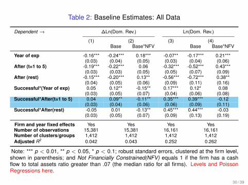
Table 2: Baseline Estimates: All Data
Dependent → ∆Ln(Dom. Rev.) Ln(Dom. Rev.)
(1) (2) (3) (4)Base Base*NFV Base Base*NFV
Year of exp -0.16*** -0.24*** 0.18*** -0.07** -0.17*** 0.21***(0.03) (0.04) (0.05) (0.03) (0.04) (0.06)
After (t=1 to 5) -0.19*** -0.22*** 0.06 -0.32*** -0.52*** 0.43***(0.03) (0.03) (0.05) (0.05) (0.07) (0.09)
After (rest) -0.15*** -0.20*** 0.13** -0.56*** -0.72*** 0.38**(0.04) (0.05) (0.06) (0.09) (0.11) (0.16)
Successful*(Year of exp) 0.05 0.12** -0.15** 0.17*** 0.12* 0.08(0.03) (0.05) (0.07) (0.04) (0.06) (0.08)
Successful*After(t=1 to 5) 0.04 0.09** -0.11** 0.35*** 0.39*** -0.12(0.03) (0.04) (0.06) (0.06) (0.09) (0.11)
Successful*After(rest) -0.05 0.01 -0.13** 0.45*** 0.44*** -0.03(0.03) (0.05) (0.07) (0.09) (0.13) (0.19)
Firm and year fixed effects Yes Yes Yes YesNumber of observations 15,381 15,381 16,161 16,161Number of clusters/groups 1,412 1,412 1,412 1,412Adjusted R2 0.042 0.043 0.252 0.262
Note: *** p < 0.01, ** p < 0.05, * p < 0.1; robust standard errors, clustered at the firm level,shown in parenthesis; and Not Financially Constrained(NFV) equals 1 if the firm has a cashflow to total assets ratio greater than .07 (the median ratio for all firms). Levels and PoissonRegressions here.
30 / 39

Table 3: Matched Estimates: Probability of Going Out of Business
Dependent= Exit All Survived SR Surv. SR & MR
Successful -0.31*** -0.26*** -0.03(0.04) (0.04) (0.02)
SuccessfulxNFV 0.08 0.07 -0.02(0.05) (0.05) (0.03)
Domestic -0.06* -0.07* -0.00(0.04) (0.04) (0.03)
DomesticxNFV 0.00 0.02 -0.02(0.05) (0.05) (0.03)
Not Fin. Vulnerable (NFV) -0.10*** -0.09** 0.01(0.04) (0.04) (0.02)
Avg. Domestic Revenuet<0 -0.03*** -0.02** -0.01(0.01) (0.01) (0.01)
Avg. Short-Term Debtt<0 0.02* 0.02 0.01(0.01) (0.01) (0.01)
Avg. Short-Term Investmentt<0 0.11*** 0.12*** 0.03(0.03) (0.03) (0.03)
Number of observations 1,468 1,391 1,165Adjusted R2 0.197 0.175 0.105
Note: *** p < 0.01, ** p < 0.05, * p < 0.1. Robust standard errors in parenthesis.The regressions also control for industry, export cohort match, short-term labor,long-term labor, inventory, property, Long-Term Investment, Long-Term Debt, andintangible. 31 / 39

Table 4: Matched Estimates: All Data
Dependent → ∆Ln(Dom. Rev.) Ln(Dom. Rev.)
Base Base*NFV Base Base*NFV
Year of Exp. -0.14*** -0.23*** 0.20*** -0.09*** -0.20*** 0.24***(0.03) (0.04) (0.05) (0.03) (0.04) (0.06)
After (t=1 to 5) -0.18*** -0.21*** 0.06 -0.36*** -0.58*** 0.47***(0.03) (0.04) (0.05) (0.05) (0.08) (0.10)
After (t=rest) -0.14*** -0.19*** 0.10* -0.57*** -0.75*** 0.42**(0.04) (0.05) (0.06) (0.10) (0.11) (0.18)
Successful*Year of Exp. -0.00 0.07 -0.05 0.23*** -0.00 0.09(0.04) (0.07) (0.09) (0.05) (0.07) (0.10)
Successful*After(t=1 to 5) 0.04 0.12*** -0.11 0.47*** 0.31*** -0.22(0.03) (0.05) (0.07) (0.07) (0.11) (0.14)
Successful*After(t=rest) -0.07* 0.11** -0.19** 0.55*** 0.36** -0.29(0.04) (0.06) (0.08) (0.11) (0.14) (0.24)
Domestic*Year of Exp. 0.04 0.09 -0.19** 0.02 0.21*** -0.01(0.05) (0.06) (0.08) (0.05) (0.07) (0.09)
Domestic*After(t=1 to 5) 0.07** 0.10** -0.12* 0.19*** 0.57*** -0.25*(0.03) (0.05) (0.06) (0.07) (0.11) (0.13)
Domestic*After(t=rest) 0.03 -0.01 -0.13* 0.22* 0.61*** -0.18(0.04) (0.06) (0.07) (0.11) (0.15) (0.22)
Firm and year fixed effects Yes Yes Yes YesNumber of observations 15,332 15,332 16,830 16,830Number of clusters/groups 1,473 1,473 1,473 1,473Adjusted R2 0.033 0.034 0.252 0.260
Note: *** p < 0.01, ** p < 0.05, * p < 0.1; robust standard errors, clustered at thefirm level, shown in parenthesis; and Not Financially Constrained(NFV) equals 1 if thefirm has a cash flow to total assets ratio greater than .07 (the median ratio). Levelsand Poisson Regressions here. 32 / 39
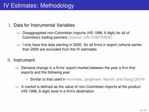
IV Estimates: Methodology
I. Data for Instrumental Variables
⇒ Disaggregated non-Colombian imports (HS 1996, 6 digit) for all ofColombia’s trading partners (Source: UN COMTRADE)
⇒ I only have this data starting in 2000. So all firms in export cohorts earlierthan 2000 are excluded from the IV estimates
II. Instrument
⇒ Demand change in a firms’ export market between the year a firm firstexports and the following year
– Similar to that used in Hummels, Jørgensen, Munch, and Xiang (2014)
⇒ A market is defined as the value of non-Colombian imports at the product(HS 1996, 6-digit) level in a firm’s destination
33 / 39

Table 5: First Stage: Probability of Going Out of Business
Dependent = Successful All Survived SR Survived SR and MR
Demand Change -0.0011** -0.0011** -0.0056(0.0005) (0.0005) (0.0102)
Number of observations 904 870 720
Note: *** p < 0.01, ** p < 0.05, * p < 0.1. Robust standard errors inparenthesis. The regressions control for industry, export cohort, and initialdomestic revenue. Angrist-Pischke multivariate F test of excluded instru-ments is 5.13/4.93/0.30.
34 / 39

Table 6: IV Estimates: Probability of Going Out of Business
Dependent = Exit All Survived SR Survived SR and MR
Successful -2.64** -2.73** 0.07(1.20) (1.26) (0.55)
Number of observations 904 870 720
Note: *** p < 0.01, ** p < 0.05, * p < 0.1. Robust standard errors inparenthesis. The regressions control for industry, export cohort, and initialdomestic revenue.
35 / 39

Table 7: First-Stage Regressions for Demand Changes as a Instrument
Dependent → A(t=0)*Suc. A(t=1-5)*Suc. A(rest)*Suc. A(t=0)*Suc. A(t=1-5)*Suc. A(rest)*Suc.
After(t = 0) 0.58*** -0.01*** -0.00 0.58*** -0.01*** -0.00*(0.02) (0.00) (0.00) (0.02) (0.00) (0.00)
After(t = 1 to 5) 0.01** 0.62*** -0.00 0.01** 0.61*** -0.00(0.00) (0.02) (0.00) (0.00) (0.02) (0.00)
After(rest) 0.01 -0.02 0.76*** 0.00 -0.04** 0.76***(0.00) (0.02) (0.02) (0.01) (0.02) (0.02)
After(t = 0)*IV -0.002*** 0.0002** -0.00002 -0.002*** 0.0002 -0.00002(0.00) (0.00) (0.00) (0.00) (0.00) (0.00)
After(t = 1 to 5)*IV 0.0002 -0.00*** -0.00002 0.0001 -0.002*** -0.00003(0.00) (0.00) (0.00) (0.00) (0.00) (0.00)
After(rest)*IV -0.002 -0.01 0.015 -0.002 -0.01 0.02(0.00) (0.01) (0.01) (0.00) (0.01) (0.01)
Observations 10,207 10,207 10,207 9,581 9,581 9,581Adjusted R2 0.542 0.613 0.735 0.542 0.613 0.734
Second-stage ln(Domestic Revenue) Domestic Revenue Growth
Note: *** p < 0.01, ** p < 0.05, * p < 0.1; All regression include firm fixed effects and year fixedeffects. Robust standard errors, clustered at the firm level, in parenthesis. Angrist-Pischke multi-variate F test of excluded instruments for Log(dom. Rev.)/ ∆log(dom. Rev.): Successful*(Year ofexp) = 48.44/45.27, Successful*After(t=1 to 5) = 12.54/12.04, Successful*After(rest) = 1.1/1.34.
36 / 39

Table 8: IV Estimates: All Data
Dependent → Ln(Dom. Rev.) ∆Ln(Dom. Rev.)
Year of exp -0.13* -0.31***(0.08) (0.11)
After(t = 1 to 5) -0.66*** -0.60***(0.25) (0.17)
After(rest) 0.23 -0.03(1.88) (0.72)
Successful*Year of exp 0.26* 0.32(0.14) (0.20)
Successful*After(t = 1 to 5) 0.90** 0.74***(0.40) (0.28)
Successful*After(rest) -0.60 -0.16(2.48) (0.96)
Firm and year fixed effects Yes YesNumber of observations 10,207 9,581Number of clusters/groups 904 904
Note: *** p < 0.01, ** p < 0.05, * p < 0.1; All regression include firmfixed effects and year fixed effects. Robust standard errors, clustered atthe firm level, in parenthesis.
37 / 39

IV. Conclusion and Future Work

Conclusion
I. Showed, theoretically and empirically, that export failure can lead tonegative domestic-market outcomes
II. For failed exporters, exporting is associated with the following:
⇒ lower domestic revenue
⇒ slower domestic growth
⇒ higher probability of going out of business
III. Implications: The uncertainty in export costs, not just export failure,might lead to fewer firms exporting.
IV. Policy implications: focus beyond market entry and lowering foreigntrade barrier
⇒ subsidize the cost of finding a good match (e.g. USITA)
⇒ lowering the cost of financing exports (e.g. EX-IM Bank)
38 / 39

Conclusion: Future Work
I. Short Term: Modify question
⇒ Are there negative consequences to exporters that try to enter anew foreign market and fail?
II. Long Term: Export failure in a general equilibrium framework
⇒ Does export failure limit the number of exporters and aggregateexports?
⇒ Likewise, does it hamper aggregate productivity gains through aninefficient allocation of resources? learning by exporting?
39 / 39

Thank You!
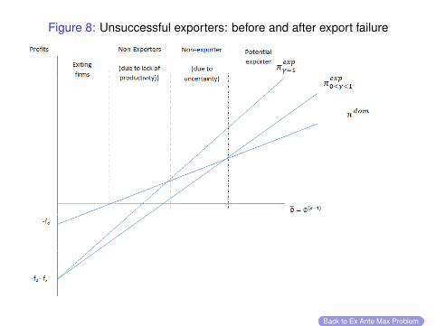
Figure 8: Unsuccessful exporters: before and after export failure
Back to Ex Ante Max Problem

Unconstrained Firms
The maximization problem for unconstrained, unsuccessful exporters:
maxpi ,Li
Eπi(φi) = LiAp1−σi −
LiAp−σiφi
− fx − fd − Lβi
The profit-maximizing price:
p∗i =σ
σ − 11φi
=µ
φi(1)
The profit-maximizing marketing expenditure:
L∗i =
(Aσβ
) 1β−1(µ
φi
) 1−σβ−1
(2)
2 / 25

Financially-constrained Firms
I. The liquidity constraint binds with the choice of L∗i and p∗i forfinancially-constrained firms
⇒ That is, piqi − qiφi
= Bi
II. To find the firm at the unconstrained/constrained threshold:
⇒ substitute L∗i and p∗i into the firm’s liquidity constraint
⇒ bind the constraint and substitute in the creditor’s constraint
⇒ solve for φi
Back to Setup
3 / 25

Exporting Makes Some Firms Financially Constrained
The financially-constrained cutoff for non-exporters:
φdomC = µ
(Aσβ
) 11−σ(
fd − (1− λ)feλβ − 1
) 1−ββ(1−σ)
(3)
For successful exporters in N markets:
φsuccC = µ
(Aσβ
) 11−σ(
Nfx + fd − (1− λ)fe(N + 1)(λβ − 1)
) 1−ββ(1−σ)
(4)
For unsuccessful exporters:
φfailC = µ
(Aσβ
) 11−σ(
fx + fd − (1− λ)feλβ − 1
) 1−ββ(1−σ)
(5)
Proposition 1: As a result of exporting, both successful and failedexporters are more likely to become financially constrained:φfail
C > φsuccC > φdom
C4 / 25

Credit-constrained Firms
I. Firms reduce financing need by choosing a lower Li (i.e. Li < L∗i )
II. How does a lower Li loosen the constraint?
⇒ The Firm’s Liquidity Constraint: piqi − qiφi≥ Bi
– Substituting and simplifying: Li Aσ
(µφi
)1−σ≥ Lβi +fx +fd−(1−λ)fe
λ
⇒ A decrease of Li ,
– lowers net revenue by ∂LHS∂Li
= − Aσ
(µφi
)1−σ
– lowers the loan repayment by ∂RHS∂Li
= −βLβ−1iλ
– credit constraint loosens when ∂RHS∂Li
< ∂LHS∂Li
.
⇒ Credit constraint loosens as Li decreases away from L∗i
III. Since deviation from L∗i lowers profits, firms deviate as little aspossible from L∗i
5 / 25
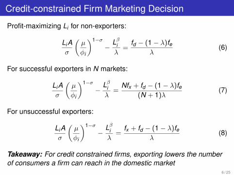
Credit-constrained Firm Marketing Decision
Profit-maximizing Li for non-exporters:
LiAσ
(µ
φi
)1−σ−
Lβiλ
=fd − (1− λ)fe
λ(6)
For successful exporters in N markets:
LiAσ
(µ
φi
)1−σ−
Lβiλ
=Nfx + fd − (1− λ)fe
(N + 1)λ(7)
For unsuccessful exporters:
LiAσ
(µ
φi
)1−σ−
Lβiλ
=fx + fd − (1− λ)fe
λ(8)
Takeaway: For credit constrained firms, exporting lowers the numberof consumers a firm can reach in the domestic market
6 / 25
Lower Bound for Li in the Domestic Market
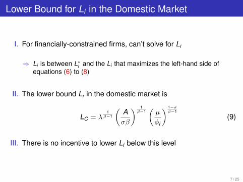
I. For financially-constrained firms, can’t solve for Li
⇒ Li is between L∗i and the Li that maximizes the left-hand side ofequations (6) to (8)
II. The lower bound Li in the domestic market is
LC = λ1
β−1
(Aσβ
) 1β−1(µ
φi
) 1−σβ−1
(9)
III. There is no incentive to lower Li below this level
7 / 25

Exporting May Lower Domestic Revenue
I. Domestic revenue for all firms is vi = piqi = LiA(µφi
)1−σ
II. Domestic revenues for unconstrained firms (Li = L∗i ):
v∗i = Aββ−1
(1σβ
) 1β−1(µ
φi
)β(1−σ)β−1
(10)
III. Domestic revenues for constrained firms will be between L∗i and alower bound, LC :
vC = Aββ−1
(λ
σβ
) 1β−1(µ
φi
)β(1−σ)β−1
(11)
Proposition 2: As a result of exporting, financially-constrainedfirms—irrespective of their success abroad—have lowerdomestic revenues: v fail
i , vsucci < vdom
i8 / 25

Firm Production/Exit Cutoff
I. Some ex ante profitable firms are unable to produce at home
⇒ Even if all profits when to the creditor, the creditor still does not breakeven.
II. The cutoff is defined by the constrained firm, φ0, whose Li choiceequals LC (Eg. 9).
9 / 25
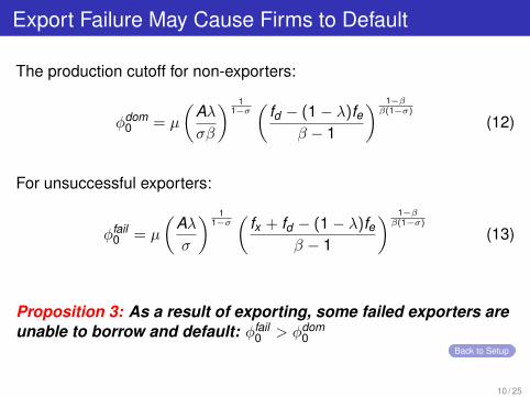
Export Failure May Cause Firms to Default
The production cutoff for non-exporters:
φdom0 = µ
(Aλσβ
) 11−σ(
fd − (1− λ)feβ − 1
) 1−ββ(1−σ)
(12)
For unsuccessful exporters:
φfail0 = µ
(Aλσ
) 11−σ(
fx + fd − (1− λ)feβ − 1
) 1−ββ(1−σ)
(13)
Proposition 3: As a result of exporting, some failed exporters areunable to borrow and default: φfail
0 > φdom0
Back to Setup
10 / 25
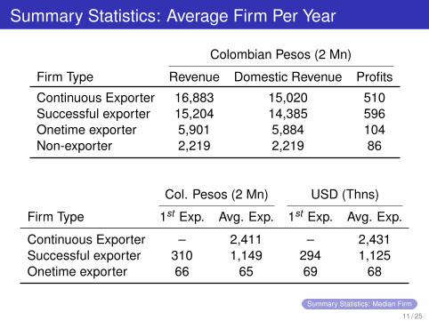
Summary Statistics: Average Firm Per Year
Colombian Pesos (2 Mn)
Firm Type Revenue Domestic Revenue Profits
Continuous Exporter 16,883 15,020 510Successful exporter 15,204 14,385 596Onetime exporter 5,901 5,884 104Non-exporter 2,219 2,219 86
Col. Pesos (2 Mn) USD (Thns)
Firm Type 1st Exp. Avg. Exp. 1st Exp. Avg. Exp.
Continuous Exporter – 2,411 – 2,431Successful exporter 310 1,149 294 1,125Onetime exporter 66 65 69 68
Summary Statistics: Median Firm
11 / 25
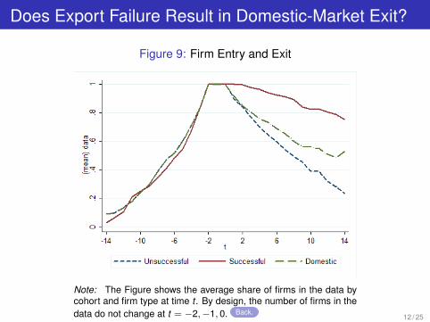
Does Export Failure Result in Domestic-Market Exit?
Figure 9: Firm Entry and Exit
Note: The Figure shows the average share of firms in the data bycohort and firm type at time t . By design, the number of firms in thedata do not change at t = −2,−1, 0. Back.
12 / 25

Export Failure and Its Consequences
Back to Theoretical Propositions

Table 9: Business Classifications and availability
Tipo Descripcion Sociedad Classification In Data
1 Personas Naturales Natural Persons2 Establecimientos de Comercio Establishments of Commerce3 Soc. Limitada Private Limited Company x4 Soc. S. A. Public Limited Company x5 Soc. Colectivas Joint Ventures x6 Soc. Comandita Simple Simple Limited Partnership x7 Soc. Comandita por Acciones Limited joint-stock partnership x8 Soc. Extranjeras Foreign Companies x9 Soc. de Hecho Business Association10 Soc. Civiles Civil Society Organisations.11 Resena Ppal, Suc, Agencia ??12 Sucursal Branch13 Agencia Agency14 Emp. Asociativas de Trabajo E.A.T Associative Work Organizations15 Entidades Sin Animo de Lucro E.S.A.L. Non-Profit Entities16 Empresas Unipersonales E.U. Self-Employed Businesses x
Back to Data
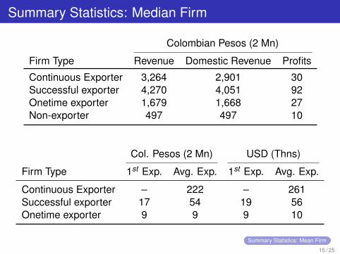
Summary Statistics: Median Firm
Colombian Pesos (2 Mn)
Firm Type Revenue Domestic Revenue Profits
Continuous Exporter 3,264 2,901 30Successful exporter 4,270 4,051 92Onetime exporter 1,679 1,668 27Non-exporter 497 497 10
Col. Pesos (2 Mn) USD (Thns)
Firm Type 1st Exp. Avg. Exp. 1st Exp. Avg. Exp.
Continuous Exporter – 222 – 261Successful exporter 17 54 19 56Onetime exporter 9 9 9 10
Summary Statistics: Mean Firm
15 / 25
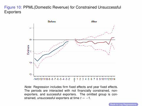
Figure 10: PPML(Domestic Revenue) for Constrained UnsuccessfulExporters
Note: Regression includes firm fixed effects and year fixed effects.The periods are interacted with not financially constrained, non-exporters, and successful exporters. The omitted group is con-strained, unsuccessful exporters at time t = −1.
Back to Log Regressions

Figure 11: PPML(Domestic Revenue), Unsuccessful vs. SuccessfulExporters
Note: Regression includes firm fixed effects and year fixed effects.The periods are interacted with not financially constrained, non-exporters, and successful exporters. The omitted group is con-strained, unsuccessful exporters at time t = −1.
Back to Log Regressions

Figure 12: PPML(Domestic Revenue), Unsuccessful Exporters vs.Non-Exporters
Note: Regression includes firm fixed effects and year fixed effects.The periods are interacted with not financially constrained, non-exporters, and successful exporters. The omitted group is con-strained, unsuccessful exporters at time t = −1.
Back to Log Regressions
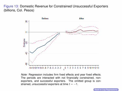
Figure 13: Domestic Revenue for Constrained Unsuccessful Exporters(billions, Col. Pesos)
Note: Regression includes firm fixed effects and year fixed effects.The periods are interacted with not financially constrained, non-exporters, and successful exporters. The omitted group is con-strained, unsuccessful exporters at time t = −1.
Back to Log Regressions
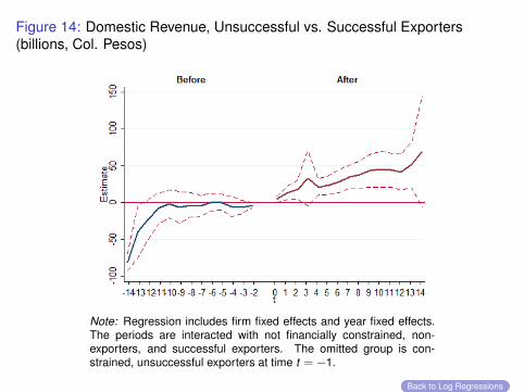
Figure 14: Domestic Revenue, Unsuccessful vs. Successful Exporters(billions, Col. Pesos)
Note: Regression includes firm fixed effects and year fixed effects.The periods are interacted with not financially constrained, non-exporters, and successful exporters. The omitted group is con-strained, unsuccessful exporters at time t = −1.
Back to Log Regressions
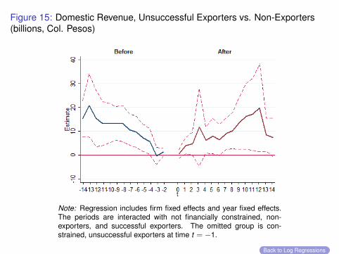
Figure 15: Domestic Revenue, Unsuccessful Exporters vs. Non-Exporters(billions, Col. Pesos)
Note: Regression includes firm fixed effects and year fixed effects.The periods are interacted with not financially constrained, non-exporters, and successful exporters. The omitted group is con-strained, unsuccessful exporters at time t = −1.
Back to Log Regressions

Table 10: Baseline Estimates: All Data
Dependent → Poisson Levels (2 billion Pesos)
(1) (2) (3) (4)Base Base*NFV Base Base*NFV
Year of exp 0.21** 0.25* -0.12 1.23 2.57 -2.88(0.10) (0.15) (0.16) (1.73) (3.54) (3.94)
After (t=1 to 5) 0.14 0.05 0.22 0.23 0.97 -1.63(0.21) (0.32) (0.41) (3.26) (6.18) (7.42)
After (rest) -0.31 -0.49 0.48 -7.66*** -7.71 0.44(0.26) (0.45) (0.51) (2.66) (4.95) (6.64)
Successful*(Year of exp) 0.03 -0.08 0.23 0.94 -1.15 4.23(0.11) (0.17) (0.19) (2.00) (3.80) (4.11)
Successful*After(t=1 to 5) 0.19 0.21 -0.10 3.96 1.07 5.67(0.23) (0.38) (0.45) (4.38) (7.08) (8.31)
Successful*After(rest) 0.57* 0.58 -0.20 11.10** 7.25 7.32(0.31) (0.50) (0.56) (4.57) (6.59) (8.53)
Number of observations 18,741 18,741 18,741 18,741Groups 1,412 1,412 1,412 1,412
Cluster by Group No No Yes YesAdjusted R2 0.019 0.019
Note: *** p < 0.01, ** p < 0.05, * p < 0.1; robust standard errors, clustered at the firmlevel, shown in parenthesis; and Not Financially Constrained(NFV) equals 1 if the firm hasa cash flow to total assets ratio greater than .07 (the median ratio for all firms).
Back to Baseline Regressions

Table 11: Baseline Estimates: Dropping Firms with 1 trillion or More Pesos
Dependent → Poisson Levels (2 billion Pesos)
(1) (2) (3) (4)Base Base*NFV Base Base*NFV
Base Base*NFV Base Base*NFVYear of exp 0.07 0.01 0.11 -0.69 -1.28* 1.08
(0.05) (0.07) (0.08) (0.62) (0.66) (0.84)After (t=1 to 5) -0.07 -0.50*** 0.80*** -2.87* -5.51*** 5.53*
(0.19) (0.18) (0.29) (1.62) (1.25) (2.96)After (rest) -0.57*** -1.12*** 1.17*** -9.84*** -12.80*** 6.91***
(0.22) (0.27) (0.33) (1.98) (2.07) (2.54)Successful*(Year of exp) 0.15** 0.15 -0.03 2.56*** 2.36* 0.31
(0.06) (0.10) (0.12) (0.86) (1.24) (1.65)Successful*After(t=1 to 5) 0.36* 0.75*** -0.76** 5.51*** 7.20*** -3.88
(0.20) (0.25) (0.34) (2.06) (2.79) (4.04)Successful*After(rest) 0.78*** 1.23*** -1.02*** 12.16*** 12.97*** -2.74
(0.23) (0.31) (0.38) (2.28) (2.83) (4.50)
Number of observations 18,718 18,718 18,718 18,718Groups 1,410 1,410 1,410 1,410
Cluster by Group No No Yes YesAdjusted R2 0.040 0.042
Note: *** p < 0.01, ** p < 0.05, * p < 0.1; robust standard errors, clustered at the firm level,shown in parenthesis; and Not Financially Constrained(NFV) equals 1 if the firm has a cash flowto total assets ratio greater than .07 (the median ratio for all firms).
Back to Baseline Regressions

Table 12: Matched Estimates: All Data
Dependent=Domestic Revenue Poisson Levels (2 billion Pesos)
Base Base*NFV Base Base*NFV
Year of Exp. 0.05 0.01 0.07 -0.18 -0.31 0.20(0.05) (0.07) (0.08) (0.60) (0.72) (0.80)
After (t=1 to 5) -0.30** -0.55*** 0.50** -3.15*** -4.32*** 2.43*(0.12) (0.18) (0.20) (0.95) (1.25) (1.46)
After (t=rest) -0.74*** -1.19*** 0.97*** -8.52*** -10.60*** 5.13**(0.19) (0.27) (0.31) (1.61) (1.83) (2.21)
Successful*Year of Exp. 0.18*** 0.22** -0.08 2.76*** 3.53** -1.42(0.07) (0.10) (0.13) (1.03) (1.69) (2.05)
Successful*After(t=1 to 5) 0.71*** 0.99*** -0.58* 10.61*** 11.89*** -2.71(0.16) (0.27) (0.31) (3.39) (4.44) (6.23)
Successful*After(t=rest) 1.13*** 1.48*** -0.81** 19.53*** 20.92*** -3.83(0.23) (0.32) (0.41) (4.53) (4.78) (8.93)
Domestic*Year of Exp. 0.00 -0.13 0.24* -0.42 -1.58** 2.87**(0.07) (0.09) (0.12) (0.61) (0.64) (1.33)
Domestic*After(t=1 to 5) 0.36** 0.48* -0.28 1.62 1.54 0.56(0.17) (0.29) (0.34) (1.30) (1.67) (2.64)
Domestic*After(t=rest) 0.59** 0.93** -0.78* 3.11* 4.03* -2.16(0.25) (0.36) (0.42) (1.71) (2.19) (3.39)
Number of observations 19,259 19,259 19,259 19,259Groups 1,473 1,473 1,473 1,473
Cluster by Group No No Yes YesAdjusted R2 0.023 0.023
Note: *** p < 0.01, ** p < 0.05, * p < 0.1; robust standard errors, clusteredat the firm level, shown in parenthesis; and Not Financially Constrained(NFV)equals 1 if the firm has a cash flow to total assets ratio greater than .07 (themedian ratio for all firms).
Back to Matching Regressions