extended benefits and the duration of ui spells: evidence from the

Journal of Public Economics 78 (2000) 107–138www.elsevier.nl / locate /econbase

Extended benefits and the duration of UI spells: evidencefrom the New Jersey extended benefit program

a,c b,c ,*David Card , Phillip B. LevineaUniversity of California at Berkeley, Berkeley, CA, USA

bDepartment of Economics, Wellesley College, Wellesley, MA 02481, USAcNational Bureau of Economic Research, Cambridge, MA, USA

Abstract

This paper examines the impact on the duration of unemployment insurance receipt of apolitically motivated program that offered 13 weeks of ‘extended benefits’ for 6 months in1996. Using state-level data and individual administrative records from before, during andafter the program, we find that it raised the fraction of claimants who exhausted theirregular benefits by 1–3 percentage points. Had the program run long enough to affectclaimants from the first day of their spell, the fraction exhausting would have risen by 7percentage points, and the average recipient would have collected regular benefits for oneextra week. 2000 Elsevier Science S.A. All rights reserved.

Keywords: Unemployment insurance; Spell duration; Extended benefits

JEL classification: J64; J65

1. Introduction

One of the key factors that may explain some of the significant gap betweenEuropean and American unemployment rates is the relative generosity of un-employment benefits. Although benefit levels tend to be somewhat higher inEurope, there is a much larger difference in the maximum duration of unemploy-ment benefits. In the United States unemployment insurance (UI) is typically

*Corresponding author. Tel.: 11-781-283-2162; fax: 11-781-283-2177.E-mail address: [email protected] (P.B. Levine).

0047-2727/00/$ – see front matter 2000 Elsevier Science S.A. All rights reserved.PI I : S0047-2727( 99 )00113-9

108 D. Card, P.B. Levine / Journal of Public Economics 78 (2000) 107 –138

available for a maximum of 26 weeks, while in many European countries themaximum duration of unemployment benefits is measured in years. Conventionaleconomic models suggest that the availability of longer UI benefits providesincentives for individuals to remain unemployed longer, contributing to the

1problems of high unemployment and long-term joblessness.In fact, existing research in the United States finds a strong positive relationship

between the maximum duration of benefits and the length of an individual’s spell2of unemployment benefits. Empirical identification in this body of work is

provided by differences in the maximum duration that occur across states and overtime. A potential difficulty with this identification strategy is that states maydecide to offer longer UI benefit durations during recessions, in response to low

3rates of job-finding that cause more individuals to exhaust their benefits. Suchendogenous policy formation may lead to an overstatement of the effect of longerUI benefits on the duration of UI spells.

In this paper we use the experiences generated by a unique legislative episode inthe state of New Jersey that led to the adoption of extended unemployment

4benefits for a 25-week period beginning on June 2, 1996. Since 1993, New Jerseyhad been using funds from its Unemployment Insurance Trust Fund to finance theindigent care costs of hospitals in the state. In the Spring of 1996, opponents ofthis financing method blocked its re-authorization, precipitating a legislative crisis.In a deal struck to gain the support of labor organizations, a law passed in May of1996 included the provision of up to 13 weeks of ‘extended’ benefits for workerswho exhausted their ‘regular’ UI benefits (those to which they are normallyentitled — typically 26 weeks). These benefits were available retrospectively toclaimants whose benefits had expired as long ago as December 1995, andprospectively to claimants who exhausted their regular UI benefits until November24, 1996.

This policy change provides two important advantages for a study of the effectof maximum benefit durations on the length of unemployment spells. First, itslegislative history makes the benefit extension unrelated to changes in thecondition of the state’s labor market. New Jersey’s economy remained robust

1See Nickell and Layard (1999) and Machin and Manning (1999) for discussions of long-termunemployment in Europe and the contribution of unemployment benefits to this phenomenon.

2See, for example, Moffitt and Nicholson (1982), Moffitt (1985), and Katz and Meyer (1990a). Thisliterature focuses on the narrow public finance question regarding the impact of maximum benefitduration on compensated unemployment spell lengths, not on total unemployment, due to dataavailability. For similar reasons, the research presented in this paper also focuses on this narrowerquestion. If one had access to similarly complete micro-data on unemployment spells, an analysis ofthese hypothetical data would better address differences in total unemployment rates across countries.

3Indeed, the federally funded extended benefit program is automatically triggered when insuredunemployment rates reach a certain threshold. The fact that benefits are typically extended during arecession would not bias the results if the econometric model controlled for the determinants of theextension (like the insured unemployment rate).

4Meyer (1992) undertakes a similar case-study approach to examine the impact of an increase in UIbenefit levels.

D. Card, P.B. Levine / Journal of Public Economics 78 (2000) 107 –138 109

throughout the period, with overall unemployment rates drifting down at about thesame rate as in nearby states. Second, the short-term nature of the New JerseyExtended Benefit (NJEB) program allows us to compare unemployment spelldurations and other outcomes during the program period with comparable datafrom immediately before and immediately after the NJEB interval.

We use two complementary sources of data for our analysis. We begin bystudying aggregated monthly data for New Jersey and other states on the fractionof UI claimants who exhaust their regular UI entitlement. Standard evaluationtechniques provide two estimates of the effect of the NJEB program: one effectwhen the program ‘turned on’; and a second when the program ‘turned off’. Oursecond data source is administrative claim records from the state of New Jerseyfrom 1995 (the year before the NJEB program) to 1997 (the year after). We usethese records to compare regular UI spell durations in the program period to spelldurations before and after. An important feature of the NJEB program is thatalmost all potential recipients of extended benefits had begun their UI spells beforethe benefit extension was announced. Standard hazard-modeling techniques allowus to compare rates of leaving UI before and after the announcement of the NJEBprogram among these ongoing spells.

Our findings suggest that the NJEB program, as enacted, had a very modesteffect on overall UI claim characteristics. Our aggregate and micro-level estimatesindicate a 1–3 percentage point increase in the fraction of claimants whoexhausted their regular UI eligibility. The impact of the policy, however, appearsto have been substantially moderated by its short-term nature. Many recipientswere well into their unemployment spell at the time the extension was im-plemented and had little opportunity to alter their behavior. Our hazard modelssuggest that the regular UI-leaving rate declined substantially (by about 15%)following the program’s introduction. Simulations of the long-term effect of abenefit extension similar to the NJEB program indicate that the availability of 13extra weeks of benefits would raise the fraction of claimants who exhaust regularUI benefits by 7 percentage points, and would raise the average duration of regularUI claims by about 1 week.

2. Review of the literature

Previous research on the effect of maximum UI eligibility on claim durationshas used data from the United States (cf. Moffitt and Nicholson, 1982; Moffitt,1985; Katz and Meyer, 1990a), Canada (Ham and Rea, 1987), Germany (Hunt,1995), and Austria (Winter-Ebmer, 1998). These studies have generally found thatan increase in the maximum duration of benefits leads to an increase in average UIspell durations. As in other policy evaluation research, an important issue in all ofthese studies is the potential endogeneity of maximum benefit durations tounobserved conditions in the labor market that also contribute to longer (orshorter) UI spells.


There are two sources of variability in maximum UI spell durations, neither ofwhich necessarily provides exogenous changes in the duration of benefits. At theaggregate level, policy changes (enacted by federal or state governments) alter theduration of benefits for all claimants. The problem with these changes is that theyare almost always triggered by slackness in the labor market that has lead to highunemployment rates, leading to a potential reversal of causality. At the individuallevel, differences in past labor market histories create differences in the maximumamount of time that different individuals can receive UI. The formula that convertsdifferences in labor market histories into different entitlement periods varies acrossstates, providing some geographic variation in maximum benefit length. However,to the extent that differences in UI entitlement are correlated with (or caused by)unobserved individual characteristics that also affect UI-leaving rates, variation inindividual-specific UI benefit durations is problematic.

Perhaps the most convincing evidence that job-finding behavior is influenced bythe maximum duration of benefits comes from an examination of the rate ofleaving the UI roles in the weeks before benefit exhaustion (cf. Meyer, 1990; Katzand Meyer, 1990b). The available data clearly indicate that the probability ofleaving UI (the hazard rate) rises sharply in the last few weeks of benefiteligibility. Although this evidence is strongly suggestive that some individualssearch harder to find a job (or return to pre-arranged jobs) just prior to benefitexhaustion, it does not directly address the policy question of the impact of abenefit extension on exit rates from UI. Moreover, results in Meyer (1990) suggestthat individuals who were already collecting UI at the time of a benefit extensionalso have a ‘spike’ in their UI-leaving rate prior to the time their benefits werepreviously scheduled to exhaust, even though they were eligible for longerbenefits.

These concerns underscore the potential usefulness of studying the effect of alegislative change in maximum benefit durations that came about at a time ofstable macroeconomic conditions, such as that generated by the NJEB program.We therefore turn to a detailed discussion of this program and its origins.

3. The New Jersey benefit extension

3.1. Overview of the UI system

The UI system in the United States is administered by the individual statesunder a set of national guidelines established by the federal government. Regular

5UI benefits are financed through a payroll tax that is mainly levied on firms. Eachstate operates a UI Trust Fund that accumulates funds during expansionary years

5Most states levy the tax exclusively on firms while some, including New Jersey, levy part of the taxon workers.


in order to finance higher expenditures in economic downturns. UI taxes arepartially ‘experience rated’: firms whose previous employees have drawn morebenefits are taxed at higher rates, subject to (often binding) minimum andmaximum rates.

Unemployed individuals are eligible to collect UI benefits if they have asufficient work history and if they remain able, available, and actively seekingwork. Weekly UI benefits are paid out according to an individual’s earnings historyprior to job loss, subject to a minimum and maximum benefit. The maximumbenefit rate varies tremendously across the states, ranging from $175 per week in

6Missouri to $365 per week in the state of Washington in 1996. New Jersey isamong the most generous states, providing a maximum benefit of $362 per weekin 1996. In contrast to the interstate variation in benefit levels, almost all states,including New Jersey, specify a maximum entitlement period of 26 weeks during

7normal economic conditions.Although regular UI benefits are usually available for up to 26 weeks, the

maximum duration of benefits is sometimes extended in cyclical downturns. Infact, since 1970 there has been a federal program that provides 13 weeks ofextended benefits when a state’s insured unemployment rate (the number ofcurrent UI claimants divided by the number of employed workers covered by thesystem) exceeds a specific threshold. Changes in the UI system over time,however, have made the trigger virtually unattainable (Blank and Card, 1991), andover the past two decades federal emergency legislation has been enacted on an adhoc basis to provide extended benefits during recessions (Blaustein et al., 1993;Woodbury and Murray, 1997). In addition, individual states can (and sometime do)raise the maximum duration of benefits. To the best of our knowledge, suchincreases have occurred exclusively during periods of adverse labor marketconditions.

3.2. ‘Charity care’ and the New Jersey benefit extension

In contrast to the traditional pattern of linking UI benefit extensions to changesin labor market conditions, the NJEB program emerged from a political com-promise around the state’s ‘Charity Care’ program for indigent hospital patients.Since its inception in 1987, the financing of this program was controversial, andover its 10-year history state legislators struggled to devise alternative financing

6These benefit levels are exclusive of dependent’s allowances which are available in some states. Theadditional payments made for each child is small in each of the handful of states which offers them.

7The maximum duration of regular benefits in most states is lower for workers with limited workhistories. Gustafson and Levine (1998) report that the average maximum duration of benefits amongyounger workers in New Jersey is between 24 and 25 weeks.


arrangements. We detail some of this turbulent history here because it illustrateshow the 1996 benefit extension came about as a short-run solution to a politicaldilemma.

In its original formulation the New Jersey Charity Care program was funded bythe Uncompensated Care Trust Fund, which collected a 19% surcharge on thehospital bills of paying patients. Soon after its introduction the surcharge cameunder fire for driving up hospital rates and insurance premiums, and lowering thenumber of individuals covered by insurance. Legislative extensions of the programbecame hotly contested and the program even expired briefly in 1989 and 1991,only to be revived shortly thereafter. In 1992, a lawsuit successfully challenged thesurcharge tax, ending this method of financing.

To replace the revenues from the surcharge, state legislators agreed to financeCharity Care by diverting some of the surplus available in New Jersey’sUnemployment Insurance Trust Fund. This plan was very unpopular among bothlabor and business groups. Labor groups worried that using funds from the TrustFund would reduce the benefits available to unemployed workers in the future.Business groups viewed the plan as a hidden payroll tax. Despite these concerns,the Charity Care program was funded in this manner from 1993 to the end of1995, when opposition grew strong enough to block an extension. However, noneof the alternatives proposed at the time, including a payroll tax, a tax on healthinsurance premiums, a tax on revenues from video poker games, and a rise in thetobacco tax, could garner enough support to be enacted. The resulting legislativegridlock led the Charity Care program to expire at the end of 1995.

Through the early months of 1996 legislators tried in vain to find ways toreinstate the program. One proposal to break the deadlock was to continue drawingfunds from the UI trust fund, but, in a gesture to organized labor, to authorize ashort-term extension in the maximum duration of UI benefits. The first referencewe have found to this proposal appears in a single sentence near the end of a NewYork Times article (March 3) on the financing crisis. Support for the proposal grewas the crisis continued; hospitals received their last payment for indigent care inFebruary and were warning of layoffs and possible hospital closures if the issuewas not resolved quickly. In the middle of May, legislation was enacted that,among other things, traded a benefit extension for the continued use of the UI trust

8fund to 1997. By the end of 1997, new legislation was enacted that graduallyeliminates the reliance on the UI trust fund by 2003, increasing the tax oncigarettes and appropriating general revenues to cover the remainder of the cost.

An examination of patterns in labor market activity by state demonstrates thatthe NJEB program was unrelated to changes in business cycle conditions. Fig. 1displays unemployment rates in New Jersey, Pennsylvania and for the entire

8A cut in the UI tax for both employers and workers was also included in the package.


Fig. 1. Monthly unemployment rate.

9United States. Recall that the period in which NJEB was in effect was June–November of 1996. Unemployment held roughly constant in New Jersey and muchof the rest of the country in 1995 before falling in 1996 and 1997. New Jersey’seconomy appeared to grow more quickly than the US as a whole over this period,but no noticeable break from trend is apparent within New Jersey or between NewJersey and other states around the period in which NJEB was in effect. As onemight expect based on the legislative history, no obvious relationship existsbetween changes in business cycle activity and the timing of the NJEB program.

3.3. Provisions of NJEB

The specific provisions of the benefit extension included a 50% increase in thenumber of weeks for which benefits could be received, equivalent to a 13-week

9The unemployment rate is not a perfect measure to use for this analysis because changes in UIpolicy may also affect the unemployment rate. Nevertheless, UI recipients represent a minority of theunemployed, and unless the impact of NJEB on spell lengths was very large its effect on the aggregateunemployment likely will be imperceptible. We have also conducted a comparison using the rates ofgrowth in employment covered by the UI system and reached similar conclusions.


extension for the large majority of recipients who were eligible for 26 weeks ofregular benefits. The extension was available to all recipients who exhausted theirregular UI benefits between June 2 and November 24 of 1996. The policy alsoapplied retrospectively to the set of claimants whose benefits expired as far back asDecember 2 of 1995, which we subsequently refer to as the ‘reachback’ group.

To collect these benefits, an exhaustee needed to return to the UI office to file aseparate claim for the extension. Formal notification letters were sent to in-dividuals in the ‘reachback’ group who had exhausted their benefits soon after thelegislation was enacted. Claimants currently receiving UI, and those who started anew claim after June 2, were not individually notified of the benefit extension untilthey received their final regular UI benefit payment. However, the state UI agencyengaged in a variety of outreach activities, including press releases, meetings withunion officials, and the like. In addition, the notification of the reachback grouppresumably generated word-of-mouth dissemination, particularly among frequentusers of the UI system.

Fig. 2 displays the take-up rate of NJEB benefits among eligible UI recipientsby the month of exhaustion of regular UI benefits. The fraction of those in thereachback group who filed a NJEB claim is about 50% among those whoexhausted regular UI in January 1996 (i.e. 5 months prior to notification ofeligibility for NJEB), and rises to about 70% among those who exhausted their

Fig. 2. Take-up rate for NJEB program by date of potential exhaustion of regular UI.


10regular benefits just prior to the law’s enactment. The take-up rate for laterclaimants (i.e. those who exhausted after the effective date of the law) remainsfairly steady at about 70% — a rate similar to estimates of the take-up rate forregular UI benefits among eligible job losers (see, for example, McCall, 1995;

11Anderson and Meyer, 1997).Nevertheless, the fact that 30% of eligible recipients did not claim NJEB raises

an issue regarding the interpretation of the results presented here. If eligibleindividuals did not take up benefits because they did not know about theiravailability, then estimates of the behavioral response to the program would bebiased downwards, relative to the expected responses from a more widelyadvertised program. We believe that this bias is unlikely to be severe, however.First, the program dissemination and application processes were similar to thoseused in other benefit extensions in New Jersey, including Emergency Unemploy-ment Compensation in the early 1990s. Although that program, in particular, didgenerate higher take-up rates than NJEB according to New Jersey officials, it wasalso offered during a recession. Evidence indicates that the most common reasonfor not applying for regular benefits among those who are eligible is theexpectation of finding a job soon (Vroman, 1991; Anderson and Meyer, 1997).Such expectations are no doubt more likely when economic conditions arefavorable and probably affect the decision to file for extended benefits as well.Second, representatives of the New Jersey Department of Labor reported to us thatwithin a few weeks of the program’s inception, recipients were well-informedabout the benefit extension. In fact, in the few weeks following the expiration ofthe program on November 24, 1996, a substantial number of recipients registeredcomplaints that they could not get it. In our empirical analysis, we investigate thispotential source of bias further by separately examining groups of workers who

10The relatively high take-up rate for NJEB among those who exhausted 6 months earlier ispotentially surprising, and suggests that many of these individuals had not found work even after 12months of joblessness.

11The slight drop-off towards the end of the NJEB window is most likely related to mistakes made indetermining a respondent’s actual exhaustion date. For an individual eligible for 26 weeks of regularbenefits, we determined his /her potential exhaustion date by moving 26 weeks forward from his /herdate of initial claim. This procedure may be inaccurate for two reasons. First, some recipients becomedisqualified for benefits for a short period during their spell because of, say, insufficient work search.These individuals may subsequently collect benefits within the same claim, but their actual date ofexhaustion will be delayed, potentially beyond the date that NJEB expired. Second, some recipientsfind temporary employment before exhausting regular benefits and then reapply for UI. Theseindividuals are eligible for the remaining number of weeks of eligibility from the initial claim, but theiractual exhaustion date will be pushed back beyond that which we predicted. In both cases, thelikelihood of incorrectly categorizing an UI recipient as eligible for NJEB increases the closer thepotential exhaustion date is to the expiration date of NJEB.


were more likely to have full information regarding the program’s existence to seeif their response is larger than that observed from other workers.

4. Empirical strategy and description of the data

The legislative history of the NJEB program makes it clear that the benefitextension was unrelated to changes in business cycle conditions in the state. Itsintroduction and ending create conditions that are ideal for a quasi-experimentalanalysis of the effect of maximum benefit durations on the behavior of UIclaimants. In fact, the short-term nature of the policy provides two opportunities toexamine the impact of higher benefit durations: one as the NJEB program began;and another when the program ended. Any effect measured at the onset of theprogram should dissipate at its expiration.

We use two different sources of data to evaluate the effects of the NJEBprogram. First, we obtained monthly data for the UI systems of all 50 states andthe District of Columbia from January 1985 to October of 1997 from the US

12Department of Labor. These state-level data contain information on the numberof initial UI claims and first payments, the fraction of claimants that exhaust theirregular benefits, and the level of covered employment in each month over thisperiod.

These data allow us to determine whether the rate of regular benefit exhaustion(defined as the number of exhaustions divided by the 6-month lag of firstpayments) increased and then returned to its previous level, during and after the

13period in which New Jersey’s extended benefits were available. We test for thepresence of such a pattern in three ways: (1) by comparing exhaustion rates inNew Jersey over time; (2) by comparing exhaustion rates in New Jersey with ratesin neighboring Pennsylvania; and (3) by comparing exhaustion rates in New Jerseywith those in the rest of the country.

Our second source of data is administrative records from New Jersey’s UIsystem for all initial claims filed between January of 1995 and December of 1997.Some 1.3 million claims were filed over this period, with first payments made to

12At the time we obtained these data in the Spring of 1998, we could only create exhaustion rates forinitial claims filed to October of 1997. Claims filed later than that had not hit their 6-month potentialmaximum duration yet. Therefore, we have no data for November of 1997 which would have beenuseful for comparison purposes with the NJEB window in 1996.

13Another possible outcome from extending the maximum duration of benefit receipt is thatindividuals who would not have applied for regular UI benefits may choose to apply. Such behavior inresponse to New Jersey’s benefit extension, however, is unlikely because the extended benefits wereonly available for about 6 months; few individuals could have filed a new claim and then exhaustedtheir regular benefits before the extension expired. Nevertheless, in preliminary data analyses, we usedthe aggregate, state-level data to test whether initial claims as a share of covered employment wasaffected by NJEB and found no statistically significant relationship.


14815 077 claimants. We restrict our attention to the subsample of claimants whoreceived a first payment, whose files include complete demographic and industryinformation, and who received no more than one week of partial UI benefits. Thelatter restriction is adopted to eliminate the small fraction of claimants who

15worked part-time while they collected UI. We also exclude all claimants youngerthan age 18 or older than 65, resulting in a useable sample of 701 743 UIrecipients.

The estimation results reported in this paper are based on the subsample of283 308 claimants whose regular UI benefits were scheduled to exhaust betweenJuly 1 and November 24 of 1995, 1996 or 1997. The period July 1–November 24,1996 includes most of the claims that were prospectively eligible for NJEB,allowing a one-month lag for information about the program to disseminate among

16claimants. We use data for those claimants scheduled to exhaust their regularbenefits from the same months of 1995 and 1997 as a ‘comparison period’, to holdconstant the seasonal differences that exist in the composition of UI claimants andin job-finding behavior. For those scheduled to exhaust regular benefits withinthese three annual windows, job-finding activity in each week of their unemploy-ment spell is analyzed, not just those weeks within the July–November period.

It is important to note that our micro-sample is limited to New Jersey UI claims.We can only use this sample to make comparisons within New Jersey over time.Thus, an assumption in most of our micro-analysis is that claims from 1995 and1997 form a valid ‘counterfactual’ for claims in 1996 (controlling for observablefactors such as unemployment rates). We provide some limited evidence on thevalidity of this assumption below.

The individual claims micro-data can be used to refine our analysis of aggregateexhaustion rates — for example, by taking into account differences acrossclaimants in the maximum duration of regular benefits. The more important use ofthe micro-data, however, is to estimate weekly hazard rates for ending a UI claimspell, and to measure the effect of NJEB eligibility on these hazard rates. Because

14Individuals who file an initial claim but do not receive a first payment include those who find a jobduring the waiting week, who are deemed ineligible for benefits after filing a claim, or who find a jobduring the period in which eligibility is being determined among those for whom eligibility has beenquestioned.

15See McCall (1996) for discussion of the set-aside provisions that allow UI recipients to workpart-time and collect some benefits. We include claimants who collect one week of partial paymentsbecause recipients frequently obtain employment in the middle of the week and their last payment is apartial one. As discussed in more detail below, a limitation of the data available to us is that we cannotidentify those respondents whose first weekly payment was a partial one.

16Restricting the sample to those whose regular benefits were scheduled to expire after July 1 of eachyear provides another advantage in that many claimants whose regular benefits would expire in June of1995 would have filed their claim at the end of 1994 since most are eligible for 26 weeks of benefits.None of these claims are available in our data and their omission could affect the comparability acrossyears. Nevertheless, some recipients whose regular benefits did not expire until after July 1, 1995 mayhave also initially filed their claim in 1994 (due to, say, a period of disqualification during the spell).


of the limited timeframe of the NJEB program, the vast majority of UI claims17affected by NJEB were in progress in June 1996. The NJEB intervention

therefore affected different individuals differently, depending on how many weeksthey had been on UI at the announcement of the program. Such a ‘time-varying’intervention is most easily modeled in the context of a conventional hazard model.

A second use of the individual claims data is to examine the effect of the NJEBprogram on the ‘spike’ in UI exit rates just prior to exhaustion of regular UIbenefits. To the extent that this spike reflects a behavioral response to theimpending cut-off in benefits, one might expect a smaller spike among claimantswho were eligible for NJEB than among claimants in the comparison group.(Although, as noted earlier, Meyer (1990) did not find much evidence of such achange).

5. Results

5.1. Analysis of aggregate data

Fig. 3 graphs aggregate monthly exhaustion rates between 1995 and 1997 forNew Jersey, Pennsylvania, and the entire United States. One obvious differenceacross these geographic entities is that the average exhaustion rate is higher in

18New Jersey. The ratio of exhaustions to 6-month lagged first payments hoversaround 50% in New Jersey compared to roughly 30% for Pennsylvania and 35%for the country as a whole. Nevertheless, movements in exhaustion rates tend to

19follow each other rather closely.Beginning in June of 1996, however, New Jersey’s exhaustion rate began

increasing slightly, while rates elsewhere drifted down. The New Jersey rate stoodat about 48% in June before increasing to over 50% in November of 1996 for thefirst time in over a year. No such trend appears in Pennsylvania or in the nationaldata. This relative upward trend is consistent with the expected effect of the NJEBprogram. In particular, one would expect the availability of NJEB to lead to a

17An individual could file a claim after the June 2, 1996 date, NJEB became effective and stillexhaust their regular benefits by November 24 of that year. For instance, an individual filing a claim onJune 2 who was eligible for 22 or fewer weeks could still qualify for NJEB. The number of recipientsfor whom this is true is very small.

18We graph 3-month backward-looking moving averages because the month-to-month variation inexhaustion rates is considerable, possibly overshadowing other patterns. Use of a moving averagemeans that any policy effect will not be observed as a discrete break in the trend, but will be moregradual.

19Several commentators have noted that the higher average rate of benefit exhaustion in New Jerseythan in Pennsylvania suggests that the latter may not be a good ‘control’ for analyzing the effect ofNJEB. An obvious alternative is New York. However, there is a notable outlier in the exhaustion seriesfor New York in July 1996 that makes it an unattractive choice. Other states with average exhaustionrates comparable to New Jersey are Washington DC, Montana, North Dakota and Rhode Island. Ratherthan use these states, we decided to use all the US as an alternative control.


Fig. 3. Exhaustion rate for regular UI benefits in New Jersey, Pennsylvania and US.

lower exit rate from UI for workers who had just started UI claims, as well as for20those had been on UI for longer. Such behavior would lead to a gradual rise in

the exhaustion rate, with a plateau after 26 weeks, as all those who became eligiblefor NJEB while on UI eventually exhaust. Given the short timeframe of the NJEBprogram, one would therefore expect a monotonically rising effect throughout theJune–November 1996 period. In the months after the benefit extension ended,exhaustions fell considerably in New Jersey, although a small decline is alsoobserved in the US as a whole.

Simple estimates of the impact of NJEB can be obtained by computing thechange in exhaustion rates in New Jersey relative to the change in other states asNJEB benefits ‘turn on’ and ‘turn off’. Such estimates are reported in Table 1. Thefirst three columns of this table present exhaustion rates in New Jersey,Pennsylvania, and the US (excluding New Jersey) for the July–November periods

21of 1995, 1996 and 1997. We use a July–November window rather than a June

20Mortensen (1977) uses a simple search model to derive the predicted effects of longer benefitavailability on search behavior of unemployed workers, and on the exit rates off UI.

21We seasonally adjusted these data using the deviation of the monthly average exhaustion ratewithin each state over the 1985–1997 period from the overall average within the state. Nevertheless,we use the same 5-month period in the preceding year because it is possible that the benefit extensionmay have affected spell lengths earlier in 1996 in anticipation of the change as the policy was beingdebated. For consistency, we report the same period in 1997, although our data only runs to October ofthat year as indicated earlier.


Table 1aUI exhaustion rates in New Jersey, Pennsylvania and the United States

Period New Penn. US DifferencesJersey except

NJ2Penn. NJ2USNJ

(1) (2) (3) (4) (5)

July–Nov. 1995 49.9 31.8 36.1 18.1 13.7(1.4) (1.2) (0.6) (1.9) (1.5)

July–Nov. 1996 49.4 29.0 33.9 20.4 15.5(1.5) (1.4) (0.6) (2.1) (1.6)

July–Oct. 1997 45.1 27.3 35.2 17.8 9.9(3.1) (1.1) (0.8) (3.2) (3.2)

199621995 20.4 22.8 22.2 2.3 1.8(2.1) (1.8) (0.8) (2.8) (2.2)

199721996 24.4 21.7 1.3 22.7 25.7(3.4) (1.8) (1.0) (3.8) (3.6)

19962Average of 2.0 20.5 21.8 2.5 3.71995 and 1997 (2.3) (1.6) (0.8) (2.8) (2.4)

a Standard errors in parentheses. Exhaustion rate represents the number of claims exhausting in amonth divided by the number of first payments 6 months earlier. The averages reported forJuly–November are weighted averages of the respective months, using as weights the number of claims(lagged 6 months). The 199621995 and 199721996 differences are simple differences of therespective averages. The entries in the last row of the table represent the difference between the 1996average and the simple average of the 1995 and 1997 averages. Data for November 1997 areunavailable.

starting date to allow for information lags during the first few weeks of the NJEBprogram. Columns (4) and (5) report the differences in exhaustion rates in NewJersey relative to the two comparison groups. As noted in Fig. 3, averageexhaustion rates are higher in New Jersey than in Pennsylvania, and also higherthan in the rest of the US as a whole.

The row labeled ‘1996 2 1995’ gives the change in exhaustion rates between the1995 and 1996 periods, while the row labeled ‘1997 2 1996’ gives the changefrom 1996 to 1997. The entries for these rows in columns (4) and (5) are the‘differences-in-differences’ in exhaustion rates between New Jersey and eithercomparison group as NJEB started and ended. Finally, the last row of the tableshows the difference in average exhaustion rate for July–November, 1996, relativeto the average for the same months in 1995 and 1997.

A number of alternative estimates of the effect of the NJEB program on NewJersey exhaustion rates can be drawn from Table 1. For example, suppose thataverage exhaustion rates would have followed a linear trend in New Jersey from1995 to 1997, in the absence of NJEB. In this case, the average of 1995 and 1997exhaustion rates is a valid counterfactual for 1996. Under this assumption, NJEBraised exhaustion rates by about 2 percentage points.

An alternative is to assume that exhaustion rates would have paralleled those in


Pennsylvania in the absence of the NJEB program. In this case, we have twoestimates of the NJEB effect: a 2.3 percentage point estimate (from the com-parison between 1996 and 1995 as NJEB ‘turned on’) and a 2.7 percentage pointestimate (from the comparison between 1997 and 1996 as NJEB ‘turned off’). Theaverage of these estimates is 2.5%, which is equivalent to the estimate formed bycomparing New Jersey in 1996 to the average of 1995 and 1997, and subtracting acomparable difference for Pennsylvania.

Finally, a third alternative is to compare New Jersey to all other states in theUS. This comparison leads to a 1.8 estimate when NJEB ‘turned on’ and a 5.7%estimate when NJEB ‘turned off’, with an average estimate of 3.7%.

These various estimates suggest that the NJEB program may have raisedexhaustion rates in the state in the July–November 1996 period by something like1–4 percentage points, although none of the estimates is statistically different fromzero. Interestingly, there is no indication from Table 1 that a simple ‘within NewJersey’ comparison [as in column (1)] gives a much different estimate of the NJEBprogram effect than a ‘difference of differences’ comparison with either Penn-sylvania or the rest of the US. Unfortunately, however, the standard errors for theestimated impacts are so large that we cannot rule out an effect of 0, or one aslarge as 6–8 percentage points.

In an effort to improve the precision of the impact estimates in Table 1, we fit aseries of regression models using monthly exhaustion rates for July–November forall the states from 1985 to 1997. These models include a full set of state and yearfixed effects that absorb permanent differences in exhaustion rates across states, as

22well as any aggregate shocks that affect all states in a given year. Five of themodels are reported in Table 2. The first specification includes only a singledummy for New Jersey observations from 1996. This model provides a validimpact estimate under the assumption that exhaustion rates in New Jersey wouldmove in parallel with the average changes in other states in the absence of NJEB.The estimated impact, 3.8%, is very similar to the averaged difference-in-differences estimate for New Jersey relative to the US as a whole in Table 1.Column (2) includes a second dummy variable for New Jersey data in 1995–1997.With this dummy included, the 1996 dummy measures the deviation of 1996 ratesfrom the average of 1995 and 1997 rates, and is therefore conceptually similar tothe averaged difference-in-difference estimate in Table 1. This change in spe-cification has little effect.

Columns (3)–(5) present models that include the state unemployment rate as acontrol variable for cyclical conditions in the labor market. This variable isstrongly correlated with exhaustion rates, and its addition significantly reduces thestandard error of the regression models, albeit at the cost of some potentialendogeneity bias. Controlling for state unemployment, the estimated impact of

22We use seasonally adjusted exhaustion rates, so we do not include month effects.


Table 2aEstimated models for monthly state exhaustion rates (July–November only)

(1) (2) (3) (4) (5)

State unemployment rate – – 3.0 3.0 3.0(0.1) (0.1) (0.1)

Dummy for New Jersey observations 3.8 3.2 0.3 2.4 2.4from 1996 (2.1) (2.5) (1.8) (2.2) (2.2)Dummy for New Jersey observations – 0.8 – 22.5 22.5from 1995, 1996 or 1997 (1.7) (1.5) (1.5)Monthly trend for New Jersey 2 2 2 2 0.1observations in 1996 only (1.2)

2R 0.65 0.65 0.73 0.73 0.73Standard error of regression 6.0 6.0 5.3 5.3 5.3

a Standard errors in parentheses. Estimated on sample of 3136 monthly observations for 49 states forJuly–November of 1985–1997. (Data for November 1997, and for Idaho and New Hampshire, areunavailable.) The dependent variable is the seasonally adjusted monthly state exhaustion rate (inpercentages). Models include unrestricted state and year effects. Monthly trend variable is normalizedto have mean 0 over the July–November 1996 period.

NJEB (i.e. the 1996 New Jersey dummy) is somewhat sensitive to the inclusion ofthe 1995–1997 dummy, although the estimates are still quite imprecise. Finally, incolumn (5) we include a monthly trend variable that increases linearly over theJuly–November 1996 period. (For ease of interpretation this trend variable has amean of 0.) This term allows us to test for any systematic trend in the relative NewJersey exhaustion rate during 1996. As suggested by the patterns in Fig. 3, theestimated trend is positive, although very imprecisely estimated.

Overall, the results in Tables 1 and 2 suggest that there was a modest increase inexhaustion rates in New Jersey during the period that UI claimants were eligiblefor extended benefits — of the order of 1–3 percentage points. However, given therather large month-to-month variability in state-level exhaustion rates, we cannotrule out an effect of 0, or one as large as 6–8 percentage points.

5.2. Analysis of administrative records

We turn now to a more detailed analysis of individual UI claim data from NewJersey during the 1995–1997 period. As noted earlier, an implicit assumptionthroughout this analysis is that claimants who were scheduled to exhaust in theJuly–November period in 1996 were comparable to those claimants in a pooled1995/1997 sample from the same months with the exception of NJEB eligibility.Weak evidence in favor of this hypothesis is provided by the similarity of theimpact estimate in Table 1 that uses only New Jersey data [i.e. the estimate in thebottom row of column (1)] to estimates that use either Pennsylvania or other USstates as a comparison group.

Some further evidence on the validity of the 1995/1997 pooled sample as a

D.

Card,

P.B.

Levine

/Journal

ofP

ublicE

conomics

78(2000)

107–138

123

Table 3aCharacteristics of UI recipients in NJ, by potential exhaustion date

July 1–November 24 Difference: 199621995/1997 average

1995 1996 1997 Difference t-statistic

Unemployment rate (county) 6.9 7.0 5.8 0.7 78.00Average weekly wage 572 567 572 25.0 3.37Replacement rate 53.7 53.9 54.5 20.2 2.79Age at claim date 38.9 39.0 39.2 0.0 1.61White (not Hispanic) (%) 64.4 62.3 60.2 0.0 0.08Black (not Hispanic) (%) 16.0 17.3 18.4 0.1 1.01Hispanic (%) 16.8 17.5 18.3 20.1 0.41Female (%) 35.2 37.0 37.8 0.5 2.86Years of education 12.26 12.27 12.27 0.0 0.66Union member (%) 15.9 15.6 14.9 0.2 1.13US citizen (%) 86.4 86.1 86.0 20.1 0.83Weeks worked for former employer 49.4 53.6 51.0 3.4 11.58

Industry distribution (%)Agriculture 2.8 2.4 2.9 20.5 7.26Mining 0.3 0.3 0.2 0.1 3.84Construction 17.4 15.5 14.9 20.7 4.45Manufacturing 19.6 18.8 17.9 0.1 0.02Transportation and public utilities 6.0 6.6 6.6 0.3 3.80Wholesale trade 8.1 8.5 8.6 0.2 0.73Retail trade 13.3 15.3 14.5 1.4 10.30Finance, insurance and real estate 5.7 4.8 4.9 20.5 5.29Public administration 2.2 2.0 2.0 20.1 2.35Services 23.9 25.1 27.2 20.5 2.91

UI claim characteristicsPercentage eligible for 26 weeks of regular UI 68.3 70.4 67.7 2.7 13.23Average weeks of UI received 17.6 16.9 16.4 20.3 1.75Percentage exhausted regular UI 48.5 47.1 42.9 0.8 7.29Percentage received NJEB 2.3 31.6 0.0 30.3 204.70Number of observations 89 226 103 492 90 590 2 2

a Samples include valid claims of individuals between ages 18 and 65 and excludes those with missing data on age, wages, industry or UI claim characteristics.


comparison for the 1996 claims sample is provided in Table 3, where we present avariety of descriptive statistics for 1995, 1996 and 1997 claims, along with t-testsfor the hypothesis that the 1996 mean is the same as the average in 1995 and

231997. The first row presents county level unemployment rates (at the firstpayment date for each claim). By this measure, economic conditions were fairly

24stable between 1995 and 1996 before improving in 1997. Other than this change,the characteristics of New Jersey UI claimants were fairly stable over our sampleperiod. Nevertheless, the large samples provide very precise estimates, so many ofthese small differences are statistically significant, as indicated by the t-statistics in

25the fifth column of the table.The bottom panel of Table 3 displays UI claim characteristics over the three

periods. Just over two-thirds of recipients are eligible for the full 26 weeks ofregular benefits in each year. The percentage of recipients that exhausted theirregular benefits in each period is very similar to the aggregate exhaustion ratesreported in Table 1, indicating that the bias introduced in the aggregated data byusing a potentially mis-measured denominator is small. A comparison of the 1996rate to the average of 1995 and 1997 indicates that the percentage of respondentsthat exhausted their regular benefits climbed 0.8 points in response to NJEB. Thisdifference may be attributable to the availability of extended benefits or,alternatively, to the relatively higher rate of unemployment in 1996 compared tothe 1995/1997 average. Almost one-third of respondents in the 1996 sample

26collected extended benefits.

23Ninety-four percent of claims that were scheduled to exhaust in the period June–November, 1996,were filed before June 2, 1996 (the effective date of NJEB). Thus, there is little likelihood that thecomposition of the claims sample was directly affected by NJEB.

24The average county unemployment rates are higher than the state averages in Fig. 1 because theadministrative records sample over-weights counties with higher unemployment. Similar weightingissues may also explain the fact that the state average unemployment rate is slightly higher in 1995 than1996, but no difference is observed here. Although one would expect the sample sizes in 1995 and1996 to be larger than that for 1997 based on the unemployment rates across years, the number ofobservations available for 1995 is diminished somewhat by the sample design. Some individuals filingan initial claim towards the end of 1994 might not receive a first payment until sometime in 1995 ifthere was some question regarding his /her eligibility for benefits and could have potential exhaustiondates between July and November of that year. Because our sample consists of initial claims filed on orafter January 1, 1995, these claimants are not in our data.

25The standard errors reported here, and in the remainder of our analysis, are subject to someunderstatement because they do not incorporate the correlation that may exist across observationswithin a particular geographic region at a point in time. In our analysis of state-level data, we estimatedcomparable models to those reported in Table 2 but controlled for the correlation across monthlyobservations within states and years and found no substantive changes in statistical inference. Forinstance, using the ‘cluster’ option in Stata to estimate the model in Table 2, column (1) actually led toa reduction in the estimated standard from 2.06 to 2.05. We address the analogous issue using themicro-data later in the paper.

26The small number of recipients in the 1995 sample window who collected NJEB were eligible byvirtue of having been temporarily disqualified for benefits during their unemployment spell, thusextending their exhaustion date beyond the potential exhaustion date we have calculated.


Table 4 presents the actual distribution of weeks of regular UI receipt for thoserecipients eligible for 26 weeks of benefits in each of the three sample periods. Theproportion of recipients who exhausted their regular benefits is somewhat smallerhere than reported in Table 3 because the full sample of spells (in Table 3)includes recipients eligible for fewer than 26 weeks of benefits, who are morelikely to exhaust. Column (4) of Table 4, which compares the 1996 frequencies tothe averages for 1995 and 1997, suggests that during the NJEB period there was a1.5 percentage point increase in the share of spells that exhausted their regularbenefits in 1996 compared to 1995 and 1997. Consistent with these findings, theshare of recipients finding jobs in weeks 13–26 is slightly lower in 1996 comparedto 1995 and 1997, indicating that some individuals may have shifted their jobfinding behavior to take advantage of the extended benefits. Again the relative

Table 4Distribution of regular UI spell lengths for those eligible for 26 weeks of benefits, by potential date of

aexhaustion

No. of weeks July 1–November 24 Difference: 199621995/1997 average

1995 1996 1997 Difference t-statistic

1 2.40 3.45 4.31 0.1 7.562 2.46 3.18 3.07 0.4 19.333 0.85 1.17 1.18 0.2 2.804 2.73 2.72 2.93 20.1 22.145 2.67 3.15 3.13 0.3 2.386 2.61 2.89 2.85 0.2 1.137 2.53 2.92 2.71 0.3 2.758 2.75 2.96 2.93 0.1 0.759 2.71 2.89 3.18 20.1 21.6310 2.86 2.82 3.15 20.2 23.2511 2.61 2.74 3.00 20.1 21.5712 2.67 2.75 2.78 0.0 20.2913 2.68 2.41 2.48 20.2 23.4314 2.40 2.22 2.43 20.2 23.1415 2.28 1.97 2.29 20.3 25.1416 2.12 1.88 2.02 20.2 23.8317 1.96 1.78 1.85 20.1 22.8318 1.93 1.69 1.92 20.2 24.5019 1.67 1.65 1.69 0.0 20.8320 1.68 1.48 1.65 20.2 23.6721 1.53 1.45 1.58 20.1 22.0022 1.63 1.47 1.53 20.1 22.3323 1.56 1.41 1.52 20.1 23.0024 1.65 1.33 1.49 20.2 25.4025 3.02 2.47 3.03 20.6 28.43

26 (exhausted) 44.06 43.15 39.30 1.5 2.57

Number of observations 62 545 72 600 62 955 – –a See note for Table 3. Samples include only those claims eligible for 26 weeks of regular UI

benefits.


frequencies are precisely estimated, and many of the differences are statisticallysignificant.

An alternative way to organize the same data is to construct the hazard rates outof UI (and the associated survivor functions) for UI recipients who were eligible

27for 26 weeks of regular benefits before, during, and after NJEB. These aregraphed in Figs. 4 and 5. As in other administrative data bases, the New Jerseysample shows a notable ‘spike’ in UI-leaving rates just prior to regular benefit

28 29exhaustion. Somewhat to our surprise, however, a fairly similar spike is alsoapparent in 1996, when NJEB was in effect. The traditional interpretation of therapid rise in UI exit rates just prior to exhaustion is that some UI recipients wait

30until the ‘last minute’ to begin a new job (or begin searching for a new job). Onthis basis, one might expect to see a much smaller spike at 25 weeks when NJEBwere available. The presence of such a strong spike in our 1996 sample suggeststhat the rise in UI-leaving rates at week 25 in the 1995 and 1997 samples may bedue in part to factors other than the strategic timing of job starting dates.

A close examination of the hazard rates in Fig. 4 reveals that although UI-exitrates in 1996 were between those in 1995 and 1997 for the first 12 weeks ofclaims, the 1996 hazard rates were lower than those in either 1995 or 1997 afterthe 13th week. Similarly, although the survivor function for 1996 claims is parallelto the function for 1997 for the first 10–12 weeks, after that point the twofunctions begin to diverge. After 13 weeks about 1.7% more claimants are still on

27An alternative approach that would utilize all spells would be to create hazard rates by ‘weeks untilexhaustion,’ which should show a spike within the few weeks prior to the regular benefit cut-off. Weexperimented with these hazards and found similar patterns to those reported here. We chose to reporthazard rates by weeks unemployed among a sample of recipients eligible for a uniform 26 weeksbecause it is easier to interpret.

28Because of data limitations, the actual spike is probably somewhat more muted than that presentedhere. All the statistics reported in this paper refer to full weeks of benefit receipt. Yet the administrativedata from which our statistics are derived enumerate calendar weeks, in which any benefit receivedduring the week is counted. Although we can largely correct for this distinction, we cannot identifythose recipients whose first calendar week of benefits was a partial week. Therefore, for some recipientsour count of full weeks of benefit receipt is overstated by one. If, for example, a claimant becameunemployed in the middle of a week and started a new job on a Monday, the measured number ofcalendar weeks of benefits received will be one higher than the number of full weeks and we are unableto correct for this. Individuals who are coded in our data as leaving UI in the week just prior to benefitexhaustion may have actually collected only 24 weeks of full regular benefits. This problem leads tosome overstatement of the pre-exhaustion exit spike. We are unsure whether a similar issue may bepresent in earlier data sets.

29The downward spike at 3 weeks reflects the fact that recipients are paid the weekly benefit for theinitial waiting week if their spell extends to 4 weeks or longer. Therefore, the marginal benefit ofremaining unemployed from the third to the fourth week is really 2 weeks’ worth of benefits, not 1.Standard search models would predict such an incentive would lower the hazard rate in the third weekand this prediction appears to be verified in the data.

30See Meyer (1990). As shown in Mortensen (1977), an optimal job search strategy in the presenceof limited duration benefits will lead to a rising exit rate as exhaustion draws near.


Fig. 4. Hazard rates out of regular UI receipt.

UI in 1996 than in 1997. But by the 25th week, this gap has risen to 4 percentagepoints.

In interpreting this apparent ‘twist’ in the 1996 hazard rate relative to the 1995or 1997 rates, it is important to keep in mind that most claim spells in our 1996sample were in progress when the NJEB program was announced. Indeed, amongthe subset of the 1996 sample eligible for 26 weeks of regular benefits, the medianclaimant would have been in his /her 13th week of UI on June 2, 1996 (had he/shenot left UI). If the announcement of NJEB caused UI claimants to reduce theirsearch intensity, one would expect to see a gradual downward shift in the average1996 hazard from earlier claim weeks (which mostly occurred before the NJEBprogram was announced) to later claim weeks (which were increasingly likely tohave occurred after the program was announced). Evidence from the hazardmodels presented below suggests that this is indeed a reasonable description of theprogram’s effect.

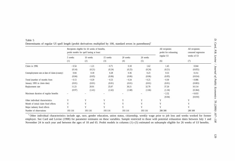
Before turning to the hazard models, however, we present a variety of simplerprobit and censored normal regression (‘Tobit-style’) models for the determinantsof the length of completed regular UI spells in our 1995–1997 samples. Thesemodels, which are presented in Table 5, can be interpreted as models for the latentduration of UI claim spells. Specifically, let y denote the amount of time ani


Fig. 5. Survivor function for regular UI spells.

individual will collect UI. The models in columns (1)–(5) of Table 5 are allmodels for the event that y exceeds a given threshold (5, 10, 15, 20 or 26 weeks)i

conditional on eligibility for 26 weeks of regular benefits. The model in column(6) describes the event that y exceeds the individual’s maximum weeks ofi

eligibility (M ), and is fit over the entire sample of claimants with potentiali

exhaustion dates between July and November of 1995, 1996 and 1997. Finally, themodel in column (7) is a censored normal regression model for y , taking intoi

account that y # M . The latter model is interesting in part because similar modelsi i

have been fit in the previous literature, allowing us to draw comparisons betweenthe New Jersey claimant sample and earlier samples.

As determinants of latent UI spell durations we include a dummy forobservations from 1996 (i.e. claimants potentially eligible for NJEB if they stayedon UI for their full entitlement period), the unemployment rate in the individual’scounty at the start of the claim, a linear trend variable (measuring months sinceJanuary 1995) to capture any generic changes in the job-finding environment inNew Jersey over time, a set of dummy variables for the month the claim started, aset of individual characteristics, including age, gender, education, union status, andcitizenship status, the individual’s average weekly wage (in the period before theclaim started) and UI replacement rate, the number of weeks worked for the

D.

Card,

P.B.

Levine

/Journal

ofP

ublicE

conomics

78(2000)

107–138

129

Table 5aDeterminants of regular UI spell length (probit derivatives multiplied by 100, standard errors in parentheses)

Recipients eligible for 26 weeks of benefits, All recipients: All recipients:

probit models for spell lasting at least: probit for exhausting censored regression

regular UI weeks of UI5 weeks 10 weeks 15 weeks 20 weeks 26 weeks

(1) (2) (3) (4) (5) (6) (7)

Claim in 1996 20.54 21.21 20.71 0.18 1.62 1.45 0.044

(0.14) (0.21) (0.24) (0.25) (0.24) (0.21) (0.055)

Unemployment rate at date of claim (county) 0.04 0.18 0.28 0.36 0.23 0.53 0.151

(0.04) (0.05) (0.06) (0.06) (0.06) (0.05) (0.014)

Trend (number of months from 20.13 20.20 20.23 20.24 20.25 20.30 20.086

January 1995 to claim date) (0.01) (0.01) (0.01) (0.01) (0.01) (0.01) (0.003)

Replacement rate 11.23 20.91 25.07 30.21 32.79 37.20 10.114

(0.97) (1.41) (1.62) (1.68) (1.66) (1.34) (0.364)

Maximum duration of regular benefits – – – – – 22.52 20.033

(0.04) (0.010)

Other individual characteristics Y Y Y Y Y Y Y

Month of initial claim fixed effects Y Y Y Y Y Y Y

Major industry fixed effects Y Y Y Y Y Y Y

Number of observations 193 116 193 116 193 116 193 116 193 116 280 308 280 308

a Other individual characteristics include age, race, gender education, union status, citizenship, weekly wage prior to job loss and weeks worked for formeremployer. See Card and Levine (1998) for parameter estimates on these variables. Sample restricted to those with potential exhaustion dates between July 1 andNovember 24 in each year and between the ages of 18 and 65. Probit models in columns (1)–(5) estimated on subsample eligible for 26 weeks of UI benefits.


previous employer, and a set of major industry fixed effects. In the models incolumns (6) and (7) we also include the individual’s maximum weeks of UI

31entitlement.The pattern of coefficient estimates for the NJEB-eligible dummy in Table 5

suggest that although UI claims with scheduled exhaustion dates after July 1, 1996were somewhat less likely to survive 5, 10 or 15 weeks than comparable spells in

]1995 and 1997, they were somewhat more likely to survive 26 weeks, or to

]]32exhaust. These findings mirror the pattern of the unadjusted survivor functions inFig. 5. In particular, up to about 15 weeks the survivor function for 1996 spells issomewhat below an average of the survivor functions for 1995 and 1997 (implyingthat 1996 spells were less likely to survive than spells in the pooled comparisongroup of 1995 and 1997 spells). Thereafter, however, the 1996 survivor function isabove the average for 1995 and 1997 (implying that 1996 spells were more likelyto last over 20 weeks or to exhaust than an average of 1995 and 1997 spells).

Reflecting the fact that 1996 spells were more likely to end quickly, but alsomore likely to exhaust, the estimates of the censored normal regression model incolumn (7) imply that on balance the number of weeks of regular benefits receivedby 1996 claimants was not too different from the average in 1995 and 1997.Several other aspects of the estimates from this model are also worth noting. Forexample, the estimated coefficient of the replacement rate variable implies that a10 percentage point increase in the replacement rate (e.g. from 0.4 to 0.5) wouldincrease the average duration of UI spells by about one week. This finding iscomparable to estimates in the previous literature (see, for example, Mortensen,1986; Meyer, 1990). The signs of the coefficient estimates for the censored normalmodel are consistent with those of the probit model for exhaustion, and themagnitudes of the coefficient estimates in the two models are also roughlyconsistent, suggesting that the normality assumption used in these models,although surely incorrect, does not affect the qualitative inferences from the

33models.

31In the probit model for exhaustion in column (6), note that the probability of exhaustion isp 5 P( y . M ). If y 5 x b 1 M a 1 u , and u is normally distributed with mean 0 and standardi i i i i i i i

deviation s, then p 5 F(x (b /s) 2 M (1 2 a) /s).i i i32As indicated earlier, the standard errors reported here are subject to some understatement because

they do not incorporate the correlation that may exist across observations at a point in time. This bias isprobably larger in models that exclude the county-level unemployment rate, since the latter presumablyaccounts for some of the correlation across individuals. We re-estimated some models excluding thecounty unemployment rate and found that the standard errors on our key variables were only raised by3–4% (the coefficient estimates are also not much affected), suggesting that local shocks are smallrelative to other variance components. In light of the relatively small standard errors for the estimatesof the key parameters in our models, any bias caused by common local shocks would have to be quitelarge to affect our inferences; nevertheless, readers should be aware of this potential problem.

33In principle the probit coefficients in the exhaustion model should equal the coefficients in thecensored regression model, divided by the estimated standard deviation of spells (12.6). The actualprobit coefficients are typically about 0.07–0.10 times as big as the censored regression coefficients.


As we noted in the discussion of the hazard rates and survival functions in Figs.4 and 5, most of the UI claims in our 1996 sample were actually in-progress whenthe NJEB program was announced. For this reason, it is likely that the estimates inTable 5 understate the ‘long-run’ effect of a 13-week benefit extension on thedistribution of UI claims. Moreover, there is some evidence that UI claims in our1996 sample were more likely to end early than those in a pooled sample of 1995and 1997 claims. Since the early weeks of the 1996 claims were largely before the

]]NJEB program, it seems implausible that UI-leaving behavior in these weeks wasaffected by NJEB. Rather, we conjecture that economic conditions in early 1996may have been somewhat ‘better’ than the average conditions in 1995 and 1997,leading to a somewhat higher exit rate from UI and an increase in the fractions ofclaims ending in 5 or 10 weeks in 1996, relative to the 1995/1997 comparisonsample. If true, this suggests that the estimates in Table 5 (and those in ouraggregate analysis in Tables 1 and 2) may understate even the ‘short-run’ impactof the NJEB program.

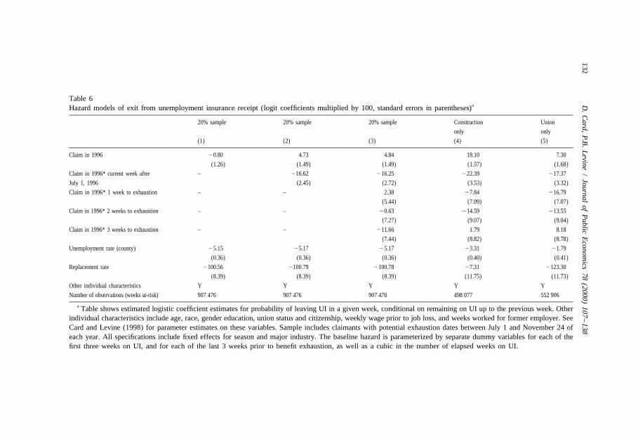
In light of the fact that almost all UI claim spells affected by the NJEB programwere in-progress in June 1996, we turn to a hazard modeling framework forrefining our estimates of the impact of the program. Specifically, we fit discrete-time hazard models for the probability l(i,t) that individual i exits UI in week t,conditional on having remained on UI up to week t 2 1. We experimented withboth conventional proportional hazard models and a simple logit functional form,

34and found very similar estimates from the two alternatives. For simplicity, wereport only the estimates from the logit specifications here. Since the probability ofexiting UI in any given week is small (3.24%), the logit coefficient estimates showthe approximate percentage change in the exit probability per unit change in theassociated covariate.

A key advantage of the hazard framework is that it allows us to measure theeffect of covariates whose values change over time, including the unemploymentrate and most importantly the presence of the NJEB program. We therefore includein our hazard models two dummy variables: one indicating spells from our 1996sample, and a second indicating whether the current week is after July 1, 1996.The former measures any differences in UI leaving rates between 1996 UI spellsand those in the comparison sample of 1995 and 1997 spells, during all weeks ofthese spells. The latter measures any differential change in UI leaving rates for the1996 spells after the NJEB program was in place (allowing a month forinformation about the program to disseminate). In this specification, any un-observed factors that happened to shift UI leaving rates in 1996 relative to theaverage rate in 1995 and 1997 will be absorbed by the 1996 spell dummy, while

34The standard proportional hazard specification is l(i,t) 5 1 2 exp(2exp( g(x ) 1 h(t))). The logiti

specification is log(l(i,t) /(1 2 l(i,t))) 5 g(x ) 1 h(t). As shown in Allison (1982), these specificationsi

are nearly equivalent when the hazard probability is low (as it is in our application). We chose toestimate logit models because of computational expedience.

132D

.C

ard,P.B

.L

evine/

Journalof

Public

Econom

ics78

(2000)107

–138

Table 6aHazard models of exit from unemployment insurance receipt (logit coefficients multiplied by 100, standard errors in parentheses)

20% sample 20% sample 20% sample Construction Union

only only

(1) (2) (3) (4) (5)

Claim in 1996 20.80 4.73 4.84 18.10 7.30

(1.26) (1.49) (1.49) (1.57) (1.68)

Claim in 1996* current week after – 216.62 216.25 222.39 217.37

July 1, 1996 (2.45) (2.72) (3.53) (3.32)

Claim in 1996* 1 week to exhaustion – – 2.38 27.84 216.79

(5.44) (7.09) (7.07)

Claim in 1996* 2 weeks to exhaustion – – 20.63 214.59 213.55

(7.27) (9.07) (9.04)

Claim in 1996* 3 weeks to exhaustion – – 211.66 1.79 8.18

(7.44) (8.82) (8.78)

Unemployment rate (county) 25.15 25.17 25.17 23.31 21.79

(0.36) (0.36) (0.36) (0.40) (0.41)

Replacement rate 2100.56 2100.79 2100.78 27.31 2123.30

(8.39) (8.39) (8.39) (11.75) (11.73)

Other individual characteristics Y Y Y Y Y

Number of observations (weeks at-risk) 907 476 907 476 907 476 498 077 552 906

a Table shows estimated logistic coefficient estimates for probability of leaving UI in a given week, conditional on remaining on UI up to the previous week. Otherindividual characteristics include age, race, gender education, union status and citizenship, weekly wage prior to job loss, and weeks worked for former employer. SeeCard and Levine (1998) for parameter estimates on these variables. Sample includes claimants with potential exhaustion dates between July 1 and November 24 ofeach year. All specifications include fixed effects for season and major industry. The baseline hazard is parameterized by separate dummy variables for each of thefirst three weeks on UI, and for each of the last 3 weeks prior to benefit exhaustion, as well as a cubic in the number of elapsed weeks on UI.


the ‘pure’ effect of the NJEB program on UI leaving behavior will be measured bythe time-varying post-NJEB coefficient.

Our hazard model estimates are presented in Table 6. For ease of computationwe selected a random 20% subset from the overall sample of UI claims withscheduled exhaustion dates from July 1–November 24 of 1995, 1996 and 1997.This sample of 56 262 claims yields a total of 932 959 claim-weeks, including25 283 ‘final payment’ weeks (weeks in which claimants exhaust their UI

35entitlement), which are treated as right-censored observations. The risk set forour hazard analysis therefore contains 907 476 observations. In light of the timepattern of the hazards shown in Fig. 4, we include a variety of controls for the‘baseline’ exit probabilities: dummies for the first 3 weeks of regular UI receipt; acubic in the number of elapsed weeks of regular UI receipt; and dummies for each

36of the last 3 weeks prior to regular benefit exhaustion. We also experimentedwith a variety of other controls, including linear and quadratic terms for thenumber of weeks remaining until exhaustion. The addition of such terms hadessentially no effect on the estimates of the NJEB program impacts nor of theeffects of the other covariates.

The specification in column (1) includes a single dummy variable for 1996claims, along with the same set of individual covariates used in the models inTable 5. The estimate of the 1996 effect is negative, but small, and statisticallyinsignificant. The effects of the control variables are typically significant, andconsistent with the signs of the coefficients of the models in Table 5.

The specification in column (2) adds the second dummy variable which equals 1for 1996 claim weeks after July 1. In this model the ‘1996’ effect is positive —indicating a 4.7% higher exit rate among 1996 spells than in the comparisonsample of 1995 and 1997 spells — while the ‘post-NJEB’ effect is negative —indicating a 16.6% drop in the UI leaving rate once the NJEB program was inplace. The pattern of these estimates provides a simple interpretation of theaverage hazards graphed in Fig. 4 and the probit results in Table 5. Specifically,the positive coefficient for 1996 spells suggests that prior to passage of NJEB,UI-leaving rates in 1996 were slightly higher than those in the 1995/1997 sample.On average, the earlier weeks in the 1996 claims sample occurred prior to NJEB,and the overall hazard rate was above the average 1995/1997 rate (as shown inFig. 4), leading to somewhat fewer spells lasting longer than 5, 10 or 15 weeks (asshown by the probit models in Table 5). The availability of NJEB, however, led toa drop in UI leaving rates, causing a gradual drop in the average hazard among

35For individuals who contributed two or more claims to our sample, we included only the firstclaim. This eliminated about 2% of all claims.

36We also estimated models on the subset of individuals eligible for 26 weeks of regular benefits thatincluded dummies for each individual week of regular UI receipt. Such a specification would becomparable to the semi-parametric proportional hazards model estimated by Meyer (1990). Again, theestimates of the key coefficients are similar.


later weeks in the 1996 (which were more and more likely to have occurred afterJune), and leading to an increase in the fraction of spells that exhausted (as shownby the probit models for exhaustion).

The model in column (3) adds three additional variables, representing interac-tions of the post-NJEB dummy with the dummies for periods 1, 2 and 3 weeks justprior to regular benefit exhaustion. The estimated coefficients on these interactionterms are small and individually and jointly insignificant, suggesting that availabil-ity of NJEB led to only small changes in the size of the ‘spike’ in exit rates prior

37to exhaustion.The models in Table 6 all ignore the presence of unobserved individual-specific

38heterogeneity. To get some sense of the possible implications of this omission,we performed a number of checks. First, we estimated the models without anyindividual-specific covariates, to gauge the sensitivity of our estimates to observ-able heterogeneity. This yielded estimates of the remaining baseline and NJEBcoefficients very similar to the ones from the richer specifications reported in thetable. For example, with no individual-specific controls, the estimate of the 1996dummy in a specification similar to the one in column (2) is 7.4 (vs. 4.7 with allcontrols), while the estimate of the post-NJEB dummy is 218.7 (vs. 216.6 withall controls). These results suggest that our estimates are not very sensitive tocontrolling for observed heterogeneity and, therefore, may not be terribly sensitiveto unobservable heterogeneity either. Second, we compared the observablecharacteristics of individuals ‘at risk’ to leave UI after various numbers of weeks.These comparisons show surprisingly little systematic trend with time on UI. Forexample, average education is 12.3 years in week 1, 12.3 years in week 12, and12.4 years one week prior to exhaustion of regular benefits. Similarly, the meanlog average weekly wage (for the old job) is 6.16 in week 1, 6.14 in week 12, and6.13 one week prior to exhaustion. Based on these results for the observablecovariates, we think it is unlikely that unobserved characteristics lead to much biasin our estimates of the impact of NJEB.

Another concern with the results in Table 6 is that our estimates of the impact ofNJEB are heavily based on the effect of NJEB on later weeks of long spells (sincethe average benefit week ‘at risk’ in the post-NJEB period of 1996 is about week15). This is only a problem, of course, to the extent that the post-NJEB effectvaries with spell duration, or varies across spells by the duration of the completedspell. To assess the possible magnitude of this type of heterogeneity, we

37In this specification, the indicator variables for the weeks immediately preceding exhaustion do notalso need to be interacted with a post-implementation dummy variable because all those eligible forNJEB with potential exhaustion dates beyond July 1 would have approached their last few weeks ofeligibility after June 2.

38Meyer (1990) considers a proportional hazards model with an unobserved individual-specificcomponent that is assumed to follow a gamma-distribution in the claimant population. The presence ofunobserved heterogeneity may lead to under-stated standard errors in the models in Table 6, and also tobias in the estimated parameters.


augmented the basic specification in column (2) with an interaction between thepost-NJEB dummy and a quadratic in the elapsed spell duration. The resultinginteractions are at best marginally significant, and show only a small increase inthe NJEB effect with elapsed duration. We also tried an ad hoc re-weightingscheme to evaluate the average effect of NJEB if the distribution of weeks at riskfor the NJEB ‘treatment’ was representative of the overall distribution of weeks atrisk to exit UI. Specifically, for each person-week ‘at risk’ to leave UI in thepost-NJEB 1996 sample, we weighted the observation by the ratio of the relativenumber of person-weeks of the same elapsed duration in the 1995/1997 com-parison sample to the relative number in the post-NJEB 1996 sample. We then fitthe duration model by weighted logit. The resulting estimate of the post-NJEBcoefficient was 217.9 (vs. the unweighted estimate of 216.6). Based on theseresults we conclude that any effects of heterogeneity in the NJEB effect are small.

As indicated earlier, another issue regarding the NJEB program is that some UIrecipients may have been unaware of their eligibility for the program. To addressthis, we replicated our analysis on two subgroups of workers that we suspect wererelatively well-informed about the program: union members (whose leaderslobbied for the extension); and workers in the construction industry (who are muchmore likely to be ‘repeat’ users of UI — cf. Meyer and Rosenbaum, 1996).Estimation results for these groups are shown in columns (4) and (5) of Table 6.Interestingly, the estimated effects of NJEB for these subgroups are quite similarto those obtained for the overall sample. In particular, the announcement of NJEBseems to have lowered exit rates by about 20% for both groups, with littleindication of any effect on the size of the ‘pre-exhaustion’ spike.

6. Discussion and conclusions

Taken as a whole the results of our analysis provide two alternative views of theeffect of the 1996 benefit extension in New Jersey. Overall, the NJEB programappears to have had a very modest impact on UI claim behavior in the state. Thefraction of recipients who exhausted regular benefits increased by about 1.5percentage points and the average spell length was largely unchanged [Table 5,columns (5)–(7)]; while the average exit rate from regular UI was only marginallyaffected [Table 6, column (1)]. Our reading of the evidence is that this modestprogram impact was due to the short-term nature of the program. Many NJEB-eligible recipients spent a large share of their unemployment spell looking forwork before NJEB was introduced. Moreover, in the absence of NJEB it appearsthat UI spells in New Jersey in 1996 would have been slightly shorter than spellsin our comparison sample of 1995 and 1997 spells. In hazard models that measurethe impact of NJEB on weeks of claim recipiency after the program wasimplemented, we find that UI-leaving rates declined significantly. Our estimates


suggest that the entire hazard profile shifted down by about 17% in each weekfollowing the onset of the extended benefit program [Table 6, column (2)].

We used this estimate to simulate the ‘long-run’ effect of a 13-week benefitextension on a pool of unemployed workers who were eligible for 26 weeks ofregular benefits and knew from the start of their spell that they could receiveextended benefits. Starting with the sample of 1997 UI claimants as a referencepopulation, we calculated claim survivor functions assuming that the weeklyhazard rates were 16.6% lower than the observed rates. The results of thesimulation suggest that the ‘long run’ effect of a 13-week extended benefitprogram would be a 7 percentage point increase in the regular UI exhaustion rate,and a roughly 1 week increase in the average number of weeks of regular UIcollected by claimants. The latter estimate of the sensitivity of weeks of regular UIreceipt to average benefit duration is lower than the estimate reported by Katz andMeyer (1990a), whose results suggest that a 13-week benefit extension should

39increase spell lengths by 2–2.5 weeks.Although the evidence from the 1996 NJEB program suggests that exit rates

from regular UI are significantly affected by a benefit extension, there is noindication that the availability of extended benefits has much affect on the rise inUI-leaving rates in the weeks just prior to the exhaustion of regular benefits. Thisfinding raises an important question regarding the cause of the pre-exhaustionspike in exit rates. It is still possible that this spike is caused by the existence of aUI system that typically offers regular benefits for 26 weeks. For instance, Topel(1983) argues that employers enter into implicit contracts with workers and cyclethem through spells of unemployment to extract the surplus created by imperfectexperience-rating in the financing of UI benefits. If the terms of the agreementinclude a 26-week spell of unemployment, then changing these contractualarrangements in response to a short-term policy may be impractical. Alternatively,workers may have been conditioned to become less selective regarding possiblejob opportunities around the time that UI typically expires. Again, a longer-termpolicy might be expected to have a bigger effect on the size of the pre-exhaustionspike than a short-term policy like NJEB. Other explanations may be available, butregardless, the evidence indicates that at least a short-term benefit extension haslittle or no impact on that spike.

These considerations also suggest that even our long-term estimates of the effectof a 13-week extended benefit program may be understated. If the program was in

39One additional explanation for the discrepancy between our estimates and those obtained in pastwork (besides the potential endogeneity bias discussed earlier) is that there may be an interactionbetween the unemployment rate and the responsiveness of a benefit extension. For instance, duringgood times, the opportunity cost of cutting back on job search activities may be too great for many andwould limit the extent to which the benefit extension would lengthen their unemployment spell.Because our study is the first that we know of that examines the impact of an increase in maximumbenefit duration during a period of economic expansion, such an interaction could explain the smallerresponse compared to earlier work. We have no evidence regarding the validity of this hypothesis.


effect for a longer time, implicit contractual arrangements could be modified,workers could be reconditioned to incorporate the longer availability of regularbenefits etc. The quasi-experiment created by the New Jersey Extended Benefitprogram provides no information on such longer-term adaptive behavior.

Acknowledgements

We thank Bruce Meyer, Roger Gordon, and two anonymous referees forcomments on an earlier draft, Tom Stengle at the US Department of Labor forproviding the monthly, state-level data employed in this analysis and Jean Behrensand Jim Phillips at the New Jersey Department of Labor for their assistance inusing the administrative records data from New Jersey. We also thank JeanBehrens for many detailed comments that substantially improved the paper. All ofthe views expressed in this paper are our own and not those of the United States orNew Jersey Departments of Labor or the National Bureau of Economic Research.

References

Allison, P.D., 1982. Discrete-time methods for the analysis of event histories. In: Leinhardt, S. (Ed.),Sociological Methodology. Josey-Bass, San Francisco.

Anderson, P., Meyer, B.D., 1997. Unemployment insurance take up rates and the after-tax value ofbenefits. Quarterly Journal of Economics 112 (3), 913–938.

Blank, R.M., Card, D., 1991. Recent trends in insured and uninsured unemployment: Is there anexplanation? Quarterly Journal of Economics 106 (4), 1157–1190.

Blaustein, S.J., Cohen, W.J., Haber, W., 1993. Unemployment Insurance in the United States: The FirstHalf Century. W.E. Upjohn Institute for Employment Research, Kalamazoo, MI.

Card, D., Levine, P.B., 1998. Extended benefits and the duration of UI spells: Evidence from the NewJersey Extended Benefits Program, Working Paper No. 6714, August, National Bureau of EconomicResearch.

Ham, J.C., Rea, Jr. S.A., 1987. Unemployment insurance and male unemployment duration in Canada.Journal of Labor Economics 5, 325–353.

Hunt, J., 1995. The effect of unemployment compensation on unemployment duration in Germany.Journal of Labor Economics 13 (1), 88–120.

Katz, L.F., Meyer, B.D., 1990a. The impact of the potential duration of unemployment benefits on theduration of unemployment. Journal of Public Economics, February.

Katz, L.F., Meyer, B.D., 1990b. Unemployment insurance, recall expectations, and unemploymentoutcomes. Quarterly Journal of Economics, November, pp. 973–1002.

Gustafson, C.K., Levine, P.B., 1998. Less-skilled workers, welfare reform, and the unemploymentinsurance system. Working Paper No. 6489, March, National Bureau of Economic Research.

Machin, S., Manning, A., 1999. The causes and consequences of long-term unemployment in Europe.In: Ashenfelter, O., Card, D. (Eds.). Handbook of Labor Economics, Vol. 4. North Holland,Amsterdam.

McCall, B.P., 1995. The impact of unemployment insurance benefit levels on recipiency. Journal ofBusiness and Economic Statistics 12, 189–198.


McCall, B.P., 1996. Unemployment insurance rules, joblessness, and part-time work. Econometrica 64(3), 647–682.

Meyer, B.D., 1990. Unemployment insurance and unemployment spells. Econometrica 58 (4), 757–782.

Meyer, B.D., 1992. Quasi-experimental evidence on the effects of unemployment insurance from NewYork State. Unpublished manuscript, February 27.

Meyer, B.D., Rosenbaum, D.T., 1996. Repeat use of unemployment insurance. Working Paper No.5423, January, National Bureau of Economic Research.

Moffitt, R., 1985. Unemployment insurance and the distribution of unemployment spells. Journal ofEconometrics 28, 85–101.

Moffitt, R., Nicholson, W., 1982. The effect of unemployment insurance on unemployment: The case offederal supplemental compensation. Review of Economics and Statistics 64 (1), 1–11.

Mortensen, D.T., 1977. Unemployment insurance and job search outcomes. Industrial and LaborRelations Review 30, 595–612.

Mortensen, D.T., 1986. Job search and labor market analysis. In: Ashenfelter, O., Layard, R. (Eds.),Handbook of Labor Economics, Vol. 2, North Holland, Amsterdam, pp. 849–920.

Nickell, S., Layard, R., 1999. Labor market institutions and economic performance. In: Ashenfelter, O.,Card, D. (Eds.). Handbook of Labor Economics, Vol. 4. North Holland, Amsterdam.

Vroman, W., 1991. The decline in unemployment insurance claims activity in the 1980s. UnemploymentInsurance Occasional Paper 91-2, January, US Department of Labor, Employment and TrainingAdministration.

Winter-Ebmer, R., 1998. Potential unemployment benefit duration and spell length: Lessons from aquasi-experiment in Austria. Oxford Bulletin of Economics and Statistics 60 (1).

Woodbury, S.A., Murray, A.R., 1997. The duration of benefits. In: O’Leary, C.J., Wandner, S.A. (Eds.),Unemployment Insurance in the United States: Analysis of Policy Issues. Upjohn Institute,Kalamazoo, MI.

extended benefits and the duration of ui spells: evidence from the

Documents