Extended Elastic Impedance using HRS-9

Brian Russell

Hampson-Russell, A CGGVeritas Company

Introduction

In a recent SEG Distinguished Lecture, Patrick Connolly outlined BP’s company-wide approach to fluid and lithology prediction using seismic data.

The cornerstones of this approach are the Coloured Inversion (CI) and Extended Elastic Impedance (EEI) methods.

This talk will first present a general framework for pre-stack and post-stack inversion methods.

I will then review the principles of EEI inversion within this framework.

Finally, I will show how the EEI method has been implemented in HRS-9, using both model-based and coloured inversion

2

Inversion in general

The above flowchart shows the general approach to seismic trace inversion, which involves a geological model, a seismic volume and an inversion algorithm. We can apply the method to either pre- or post-stack seismic data.

Geological Model

Seismic Volume

Inversion Algorithm

Inverted Seismic Volume

3

Post-stack inversion

The earliest trace inversion approach involved building an AI (acoustic impedance, or rVP) model and inverting the stacked volume to create an AI output.

AI Model Volume

Stacked Volume

Inversion Algorithm

AI Inversion

4

Model building

Building a model volume involves the following steps: Create the log property of interest at each well location

and insert it into the model (in this case, we create acoustic impedance by multiplying VP by density).

Make sure the well logs match the seismic data in time by performing correlation with an extracted wavelet.

Interpolate the logs using an algorithm such as inverse-distance weighting or kriging.

Insert the seismic picks to guide the interpolation structurally.

Apply a low pass filter (typically 0 – 15 Hz) so that the detail in the inversion will come from the seismic data.

5

6

Recursive: Bandlimited inversion, in which the seismic trace is integrated and added to the low frequency part of the model. Model Based: Iteratively updates the initial model to find a best fit to the synthetic. Sparse Spike: Constrained to produce as few events as possible, with the low frequency model added in. Coloured: Spectrum of seismic data is shaped to the well log spectrum and a 90 degree phase shift applied. In the standard implementation, no low frequencies are added back (relative impedance) but in our implementation we can add them back (absolute impedance).

These post-stack inversion methods are available in HRS-9:

Types of inversion algorithms

Gas sand stack

7

For example, here is a stack over a gas sand from Alberta, showing a “bright-spot” anomaly.

8

Post-stack inversion

AI

AI

AI= RAI

2

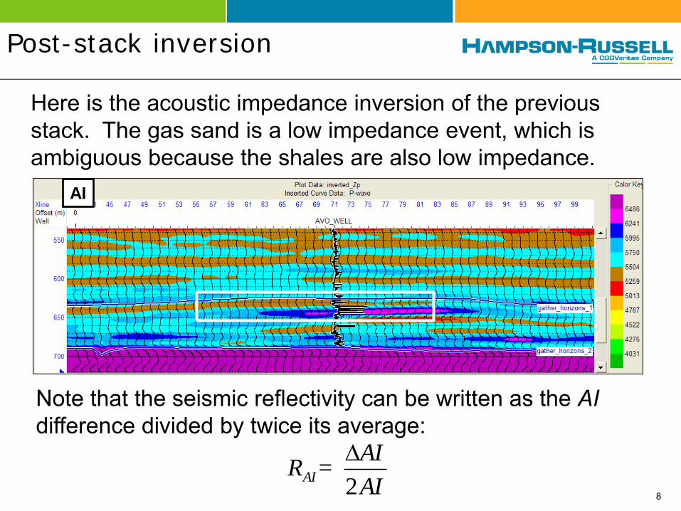
Here is the acoustic impedance inversion of the previous stack. The gas sand is a low impedance event, which is ambiguous because the shales are also low impedance.

Note that the seismic reflectivity can be written as the AI difference divided by twice its average:

Pre-stack simultaneous inversion

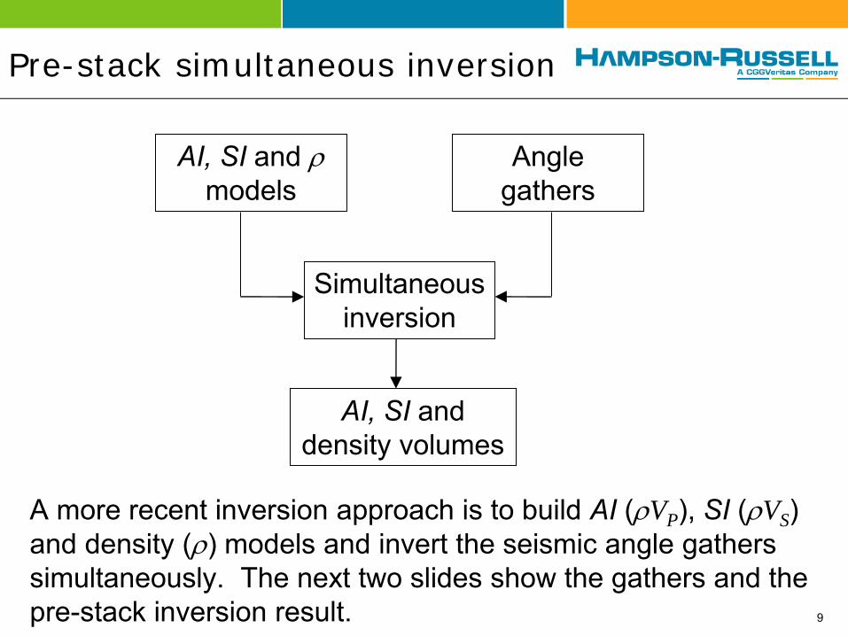
A more recent inversion approach is to build AI (rVP), SI (rVS) and density (r) models and invert the seismic angle gathers simultaneously. The next two slides show the gathers and the pre-stack inversion result.

AI, SI and r models

Angle gathers

Simultaneous inversion

AI, SI and density volumes

9

The seismic gathers

The seismic line is the “stack” of a series of CMP gathers, as shown here.

Here is a portion of a 2D seismic line showing the gas sand “bright-spot”.

The gas sand is a typical Class 3 AVO anomaly.

10

11

AI

Vp/Vs

Pre-stack simultaneous inversion

Note the unambiguous low Vp/Vs ratio at the gas sand.

12

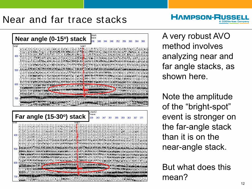
A very robust AVO method involves analyzing near and far angle stacks, as shown here. Note the amplitude of the “bright-spot” event is stronger on the far-angle stack than it is on the near-angle stack. But what does this mean?

Near and far trace stacks

Near angle (0-15o) stack

Far angle (15-30o) stack

13

Elastic Impedance

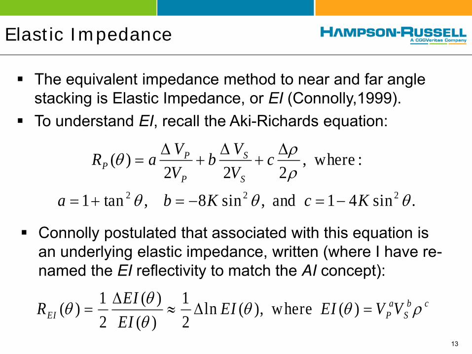
The equivalent impedance method to near and far angle stacking is Elastic Impedance, or EI (Connolly,1999).

To understand EI, recall the Aki-Richards equation:

.sin41 and ,sin8,tan1

: where,222

)(

222

r

r

KcKba

cV

Vb

V

VaR

S

S

P

PP

cb

S

a

PEI VVEIEIEI

EIR r

)( where,)(ln

2

1

)(

)(

2

1)(

Connolly postulated that associated with this equation is an underlying elastic impedance, written (where I have re-named the EI reflectivity to match the AI concept):

Elastic impedance inversion

The inversion approach for EI involves building an EI() model and inverting an angle stack volume at an angle to create an EI output.

EI() Model Volume

Angle Stack Volume

Inversion Algorithm

EI() Inversion

14

15

Here is the comparison between the EI inversions of the near-angle stack and far-angle stack. Notice the decrease in the elastic impedance value on the far-angle stack.

Gas sand case study

EI(7.5o)

EI(22.5o)

The figures show the (a) crossplot between near and far EI logs, and (b) the zones on the logs. Notice the clear indication of the gas sand (yellow).

EI from logs

(a) (b)

EI_Near EI_Far

16

17

Gas sand case study

This figure shows a crossplot between EI (7.5o) and EI (22.5o). The background trend is the grey ellipse, and the anomaly is the yellow ellipse. As shown below, the yellow zone corresponds to the known gas sand.

EI at 7.5o

EI a

t 22.

5o

18

Scaled Elastic Impedance

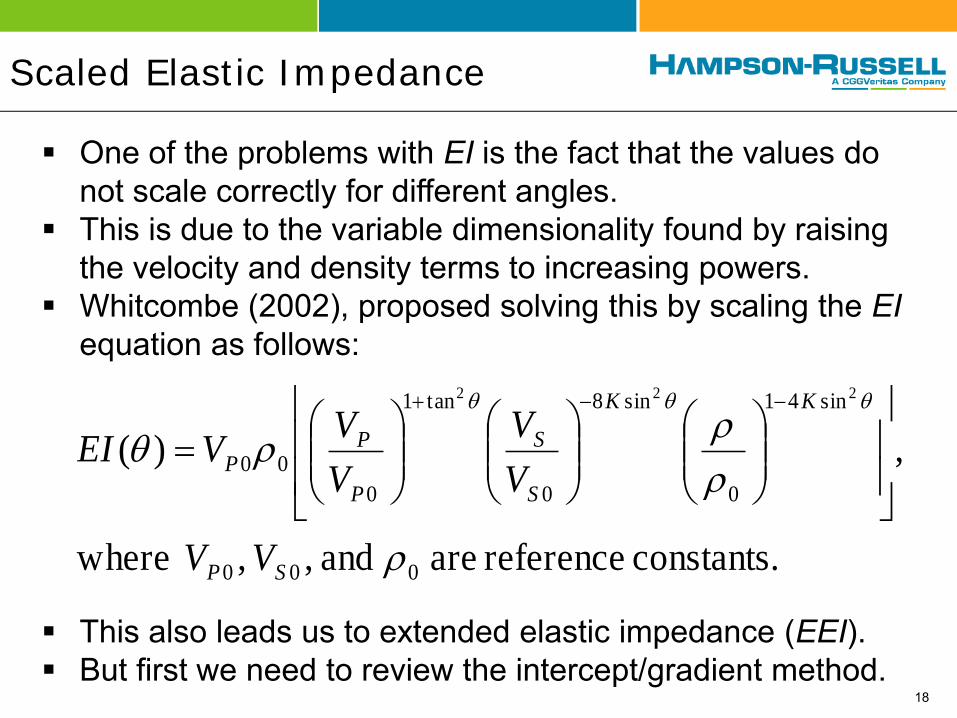
One of the problems with EI is the fact that the values do not scale correctly for different angles.

This is due to the variable dimensionality found by raising the velocity and density terms to increasing powers.

Whitcombe (2002), proposed solving this by scaling the EI equation as follows:

constants. reference are and ,, where

,)(

000

sin41

0

sin8

0

tan1

0

00

222

r

r

rr

SP

KK

S

S

P

PP

VV

V

V

V

VVEI

This also leads us to extended elastic impedance (EEI). But first we need to review the intercept/gradient method.

The Intercept/Gradient method

The Intercept/Gradient method is an approach to AVO which involves re-arranging the Aki-Richards equation to:

: w here,tans ins in)( 222 CBAR P

This is again a weighted reflectivity equation with weights of a = 1, b = sin2, c = sin2 tan2.

. and ,2

,2

42

82

,22

2

P

S

p

PVP

S

S

p

P

p

PAI

V

VK

V

VRC

KV

VK

V

VB

V

VRA

r

r

r

r

19

20

Offset +A

+B

- B

sin2

Time

The Aki-Richards equation predicts a linear relationship between these amplitudes and sin2θ. Regression curves are calculated to give A and B values for each time sample.

The amplitudes are extracted at all times, two of which are shown:

-A

The Intercept/Gradient method

21

The result of this calculation is to produce 2 basic attribute volumes

Intercept: A

Gradient: B

The Intercept/Gradient method

Extended Elastic Impedance

As the next step from scaled EI, Whitcombe et al. (2002) introduced Extended Elastic Impedance, or EEI.

First, they replaced the sin2 term in the two-term Aki-Richards equation with tanc, to give the following expression for EEI reflectivity, REEI.

22

ccccc

cc

sincoscos)()(

tan)(sin)( 2

BARR

BARBAR

EEI

P

Notice that EEI will equal acoustic impedance at c = 0o and gradient impedance (GI) at c = 90o. The limits of c are + and - 90o.

Extended Elastic Impedance

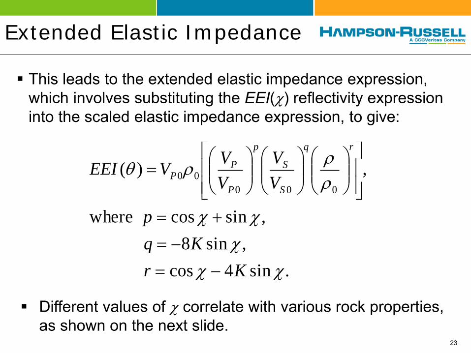
This leads to the extended elastic impedance expression, which involves substituting the EEI(c) reflectivity expression into the scaled elastic impedance expression, to give:

Different values of c correlate with various rock properties, as shown on the next slide.

.sin4cos

,sin8

,sincos where

,)(000

00

cc

c

cc

r

rr

Kr

Kq

p

V

V

V

VVEEI

rq

S

S

p

P

PP

23

Extended Elastic Impedance

Figure (a) shows EEI values at different angles and figure (b) compares elastic parameters to their equivalent EEI curves.

Whitcombe et al. (2002)

(a) (b)

24

Vp/Vs

EEI(45o)

l EEI(19o)

K EEI(10o)

m EEI(-58o)

rVs

EEI(-45o)

EEI inversion

The EEI inversion approach involves building an EEI(c) model and inverting the EEI(c) volume using an inversion algorithm to create an EEI output.

EEI(c) Model Volume

EEI(c) Volume

Inversion Algorithm

EEI(c) Inversion

25

Implementation in HRS-9

Now that we have discussed the theory of EEI, let’s see how to implement the process in HRS-9.

The process involves four steps: Choose a target log and find the optimum c angle. Build the log parameter model. Compute the EEI(c) seismic volume from the

intercept and gradient. Perform the inversion.

We have recently built this functionality into HRS-9. Since the process involves a number of steps, we will first

build a Workflow.

26

27

Creating an EEI Workflow

We start by creating a new workflow Group Name and then start the Workflow Builder.

EEI Workflow

The workflow is built by moving processes from the Process to the Workflow list. The final Workflow is on the right. 28

Gas sand case study

We will now apply this Workflow to the dataset just described.

As our target log, we have chosen the Vp/Vs ratio. Note that this will produce the same output as pre-

stack simultaneous inversion. However, the approach will be different since we are

building an EEI model and inverting the rotated intercept and gradient stacks.

In both cases, we are using the pre-stack data as input, rather than the post-stack data.

We will apply both model-based and coloured inversion.

29

First, use the AVO Attribute Volume option to create A and B:

30

Creating A and B volumes

This display is the product of A and B:

31

Correlation plot

We then find the maximum correlation value, which is at 39o with a correlation coefficient of close to 1.00. In this case, almost any value between 30o and 60o would work reasonably well. However, in some cases there is a clear peak.

A good display option is the EEI Spectrum, which shows the EEI computation for every angle between -90o and +90o. 32

EEI log spectrum

Next, we compute the EEI log at c = 39o. It closely resembles the Vp/Vs ratio log but the units are impedance. 33

EEI log curve at c = 39o

Vp/Vs Ratio

EEI at 39o

Vs Density Vp

EEI model

Next, we compute the EEI reflectivity section, as shown above (Note: REEI(39o) = A*cos(39o) + B*sin(39o))

34

EEI model

The next step is to create the filtered EEI model:

35

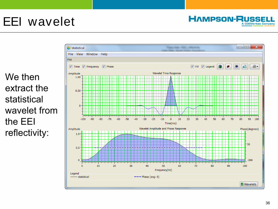
EEI wavelet

We then extract the statistical wavelet from the EEI reflectivity:

36

EEI inversion analysis

The results of post-stack inversion analysis are shown here:

37

Model-based EEI inversion

Model-based inversion with the EEI log is shown here:

38 The gas sand zone is well defined but the units are impedance.

Model-based EEI inversion

Here, we scaled to Vp/Vs units using a single scaler:

39 Now the gas sand zone has the correct low Vp/Vs values.

Coloured EEI inversion

Alternately, we apply coloured inversion, with relative scaling.

40 Note we still have an excellent definition of the gas sand.

Conclusions

This presentation has been an overview of the extended elastic impedance (EEI) approach using HRS-9.

I first reviewed post and pre-stack inversion methods. I then discussed EEI theory and how the general inversion

method could be modified to implement EEI inversion. I then showed how to find an optimum c angle to create the

EEI section. I chose Vp/Vs ratio as the target log. I then showed how to create the EEI section in HRS-9. Next, I created the inverted Vp/Vs volume, using both

model-based and coloured inversion. Both of the EEI inversion methods gave us excellent

definition of the gas sand zone, comparable to pre-stack inversion.

41