extended phase graphs (epg) - stanford...

B.Hargreaves - RAD 229

Extended Phase Graphs (EPG)

• Purpose / Definition

• Propagation

• Gradients, Relaxation, RF

• Diffusion

• Examples

133


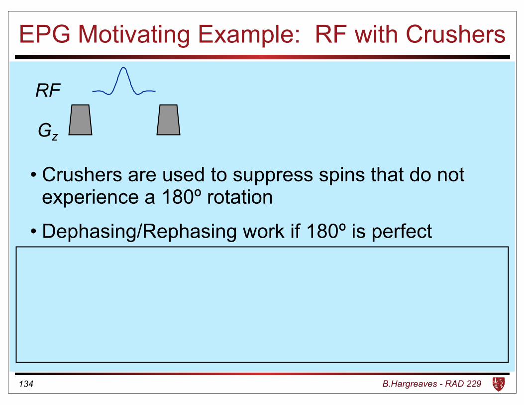
EPG Motivating Example: RF with Crushers

• Crushers are used to suppress spins that do not experience a 180º rotation

• Dephasing/Rephasing work if 180º is perfect

• Bloch simulation: Must simulate positions across a voxel, then sum all spins:

>>w = 360*gamma*G*T*z >>M = zrot(w)*xrot(alpha)*zrot(w)*M; %

134

RF

Gz



135

120xº RFGz

= +

Mx

My

Mx

My

Mx

My

Gz



• Brute-force simulation works, but little intuition

• Quantized gradients produce “dephased cycles”

• Decompose elliptical distributions to +/- circular

136

RF

Gz


Extended Phase Graphs: Purpose

Hennig J. Multiecho imaging sequences with low refocusing flip angles. J Magn Reson 1988; 78:397–407.

Hennig J. Echoes – How to Generate, Recognize, Use or Avoid Them in MR-Imaging Sequences, Part I. Concepts in Magnetic Resonance 1991; 3:125-143.

Hennig J. et al. Calculation of flip angles or echo trains with predefined amplitudes with the extended phase graph (EPG)-algorithm: principles and applications to hyperecho and TRAPS sequences. MRM 2004; 51:68-80

One cycle of phase twist from a spoiler

gradient (for example)

MxMy

137


Magnetization Vector Definitions

138

2

4M

xy

M⇤xy

Mz

3

5 =

2

41 i 01 �i 00 0 1

3

5

2

4M

x

My

Mz

3

5

2

4M

x

My

Mz

3

5 =

2

40.5 0.5 0

�0.5i 0.5i 00 0 1

3

5

2

4M

xy

M⇤xy

Mz

3

5

• Common representations for magnetization:


The EPG Basis

• Consider spins in a voxel:

–z is the location (0 to 1) across the voxel

–Mxy(z) and Mxy*(z) are the transverse magnetization

–Mz(z) is the longitudinal magnetization

• Represent the (huge) number of spins using a compact basis set of Fn and Zn coefficients

• Motivation: Propagation of the basis functions through RF, gradients, relaxation is fairly simple

139


EPG Basis: Graphical

Voxel Dimension

Z1

Voxel Dimension

Z2

Mz

Voxel Dimension

Z0

Voxe

l Dim

ensi

on

MxMy

F0

MxMy

F2

MxMy

F-1Mx

My

F1

. . .

. . .

. . .

• Fn and Zn are basis coefficients

• Transverse basis are simple phase twists (sign of n indicates direction)

• Longitudinal basis are sinusoids

MxMy

F-2

140


EPG Basis: Mathematically

Voxel Dimension

Z1

MxMy

F-1

MxMy

F1• Transverse basis functions (Fn) are just phase twists:

• Longitudinal basis functions (Zn) are sinusoids:

Although there are other basis definitions, this is consistent with that of Weigel et al. J Magn Reson 2010; 205:276-285

Fn and Zn are the basis coefficients, but we sometimes use them to refer to the basis functions they multiply

141

Mz(z) = Real

(Z0 + 2

NX

n=1

Zne2⇡inz

)

Mxy

(z) =�1X

n=�N

F ⇤n

e2⇡inz +NX

n=0

Fn

e2⇡inz


Magnetization to EPG Basis

• Positive F states (n>0):

• Negative F states (n<0):

• Z states (n>=0):

142

Fn

=

Z 1

0M

xy

(z)e�2⇡inzdz

Fn

=

Z 1

0M⇤

xy

(z)e�2⇡inzdz

Zn =

Z 1

0Mz(z)e

�2⇡inzdz

F-n


Review Question• What are the F states that represent this

magnetization (entirely along My)?

My

Mx

z

Mx(z) = 0My(z) = 2cos(2πz)

Answers: A) F1=1, F-1=1B) F1=1, F-1=iC) F1=i, F-1=i

Recall:

143


Basis Functions in MR SequencesKey Point: Basis is easily propagated in MR sequences:

•Gradient (one cycle over voxel):

– Increase/decrease Fn state number (n) or Fn+1=Fn

•RF Pulse

– Mixes coefficients between Fn, F-n and Zn

•Relaxation

– T2 decay attenuates Fn coefficients

– T1 recovery attenuates Zn coefficients, and enhances Z0

•Diffusion

– Increasing attenuation with n (described later) 144


EPG Propagation: Gradient

Voxe

l Dim

ensi

on

MxMy

F0

MxMy

F-1

MxMy

F1

MxMy

F-2

• Magnetization in Fn moves to Fn+1

–Dephasing for n>=0

–Rephasing for n<0

• Generally can apply p cycles (increase n by p)

• Z states are unaffected

Assume the “gradient” such as a spoiler or crusher induces one twist cycle per voxel

Fn+1 = Fn

Gradients induce one cycle (2π) of phase across a voxel

145


EPG Relaxation over Period T

MxMy

F-2• Transverse states:

Fn’ = Fn e-T/T2

• Zn states attenuated:

Zn’ = Zn e-T/T1 (n>0)

• Z0 state also experiences recovery:

Z0’ = M0 (1-e-T/T1 )+ Z0 e-T/T1

MxMy

F-2’

Voxel Dimension

Z1

Voxel Dimension

Z1’

Mz

Voxel Dimension

Z0

Mz

Voxel Dimension

Z0’

146


EPG RF: Transverse Effects• First consider transverse spins after

one cycle of dephasing:

• After a 60xº tip, the transverse distribution is elliptical, but can be decomposed into opposite circular twists (F1 and F-1)

F1

Mx

My

= +

F1 F-1Mx

My

Mx

My

Mx

My

Longitudinal (Zn) states are also affected – described shortly

3D view Transverse View

Transverse View

My

Mz

Mx

147


EPG RF Rotations

• An RF pulse cannot change number of cycles

• “Mixes” Fn, F-n and Zn (details next…)

Voxel Dimension

Z2

MxMy

F2

MxMy

F-2

148


EPG RF Rotations• Dephased magnetization generally has an elliptical

distribution, even after additional nutations (flips)

• Can decompose into a sum of opposite circular twists (previous slide) and cosines along Mz

• Can derive (trigonometrically) for flip angle α about a transverse axis with angle φ from Mx:

149

2

4Fn

F�n

Zn

3

50

=

2

4cos

2(↵/2) e2i� sin2(↵/2) �iei� sin↵

e�2i�sin

2(↵/2) cos

2(↵/2) ie�i�

sin↵�i/2e�i�

sin↵ i/2ei� sin↵ cos↵

3

5

2

4Fn

F�n

Zn

3

5

Same Rφ RF rotation as before, in [Mxy,Mxy,Mz]T frame


RFEffects

Phase Graph “States” (Flow Chart)

F0

Z0

F1 F2 FN. . .

Z1 Z2 ZN. . .

F-1 F-2 F-N. . .F0*

T2Decay

T1Decay

T1 Recovery

Tran

sver

se

(Mxy

)Lo

ngitu

dina

l (M

z)

Gradient Transitions

150


Examples:

• For a 90x rotation:

• (Right-handed!)

• For a 90y rotation:

• (Right-handed!)

151

2

4Fn

F�n

Zn

3

50

=

2

4cos

2(↵/2) e2i� sin2(↵/2) �iei� sin↵

e�2i�sin

2(↵/2) cos

2(↵/2) ie�i�

sin↵�i/2e�i�

sin↵ i/2ei� sin↵ cos↵

3

5

2

4Fn

F�n

Zn

3

5

Ry(⇡/2) =

2

40.5 �0.5 1�0.5 0.5 1�0.5 �0.5 0

3

5

Rx

(⇡/2) =

2

40.5 0.5 �i0.5 0.5 i

�0.5i +0.5i 0

3

5


Example 1: Ideal Spin Echo Train

RF

Gz

180xº180xº90yº

• 90 excitation transfers Z0 to F0

• Crusher gradients cause twist cycle

• Relaxation between RF pulses (Here e-TE/T2=0.81)

• 180x pulse rotation:

– Swap Fn and F-n

– Invert Zn

152

2

4Fn

F�n

Zn

3

50

=

2

40 1 01 0 00 0 �1

3

5

2

4Fn

F�n

Zn

3

5


Example 1: Ideal Spin Echo Train

RF

Gz

180xº180xº90º

Mz

Voxel Dimension

Z0

Voxe

l Dim

ensi

on

MxMy

F0

MxMy

F-1

MxMy

F1

Voxe

l Dim

ensi

on

MxMy

F0

MxMy

F-1

MxMy

F1

Voxe

l Dim

ensi

on

MxMy

F0

Signal = 0.81 Signal = 0.66

153


F0

F1

F-1

Z0

Z0

Coherence Pathways: Spin Echo

RFGz

180xº90º180xº 180xº

phas

e

time

Transverse (F)Longitudinal (Z)

F0F1

F-1

Z0

Z0

F0F1

F-1

Z0

Z0

• Diagram shows non-zero states and evolution of states

• Perfect 180º pulses keep spins in low-order statesEcho Points

154


Example 2: Non-180º Spin Echo• Ideal spin echo train gives simple RF rotations

• Now assume refocusing flip angles of 130º

• Compare RF rotations:

• Positive Fn states remain because magnetization is not perfectly reversed, generating higher order states

• Many more coherence pathways (see next slide…)

130xº180xº

155

2

40.18 0.82 �0.77i0.82 0.18 0.77i0.38i 0.38i �0.64

3

5


Coherences: Non-180º Spin Echo

RFGz

180º90º

180º 180º

Transverse (F)Transverse, but no signal

Longitudinal (Z)

phas

e

F1

F-1

Z0time

Echo Points

Only F0 produces a signal… other Fn states are perfectly dephased

F0

F1

F2

156


Example 3: Stimulated Echo Sequence

• We will follow this sequence through time

• Show which states are populated at each point

60º 60º 60º 60º

157


Example 3: Stimulated Echo Sequence

• Prior to the first pulse, all spins lie along Mz

• This is Z0=1M

z

Voxel Dimension

Z0

60º 60º 60º 60º

158


Stimulated Echo: Excitation: F0

• After a 60º pulse, transverse spins are aligned along My (F0=sin60º)

• One half (cos60º) of the magnetization is still represented by Z0

*Note that we show the “voxel dimension” along different axis for Z and F states

F0

Voxe

l Dim

ensi

on

Mz

Voxel Dimension

Z0

Mz

Voxel Dimension

Z0+

60º 60º 60º 60º

159


One Gradient Cycle

• The gradient “twists” the spins represented by F0

• We call this state F1, where the 1 indicates one cycle of phase (F1=0.86)

• The spins represented by Z0 are unaffected

F0

Voxe

l Dim

ensi

on

Mz

Voxel Dimension

Z0+

F1

MxMy

Mz

Voxel Dimension

Z0

+

60º 60º 60º 60º

160


Another Excitation (60º)

• The Z0 magnetization is again split to F0 and Z0

• The F1 magnetization is split three ways, to F1, F-1 (reverse twisted) and Z1

F1

MxMy

Mz

Voxel Dimension

Z0+ F0

Voxe

l Dim

ensi

on

Mz

Voxel Dimension

Z0+

+

F-1

MxMy

F1

MxMy Voxel Dimension

Z1

+ +

60º 60º 60º 60º

161


Another Gradient Cycle• The F-1 state is refocused to F0

• The F0 and F1 states become F1 and F2

• The Z states are all unaffected

• The process continues…!

F0

Voxe

l Dim

ensi

on

Mz

Voxel Dimension

Z0++

F-1

MxMy

F1

MxMy

Voxel Dimension

Z1

+ +

F0

Voxe

l Dim

ensi

onF2

MxMy

Voxel Dimension

Z1

F1

MxMy

Mz

Voxel Dimension

Z0

+ +

++

162


Example 3: Coherence Pathwaysph

ase

RF / Gradients

time

F0

F1

F-1

F-2

F2

Z1

Z2

Z0

Transverse (F)Longitudinal (Z)

60º 60º 60º 60º

• The stimulated echo sequence coherence diagram is shown below

• Compare with F and Z states on prior slide (location of arrow)

163


Summary of Sequence Examples

• 90º and 180º RF pulses “swap” states

• Generally RF pulses “mix” states of order n

• Gradient pulses transition all Fn to Fn+p

• Coherence diagrams show progression through F and/or Z states to echo formation

• Signal calculation examples actually quantify the population of each state

164


Matlab Formulations

• Single matrix called “P” or “FZ” (for example)

• Rows are Fn, F-n and Zn coefficients, Column each n

• RF, Relaxation are just matrix multiplications

• Gradients are shifts

165


Matlab Formulations• EPG simulations can be easily built-up using modular functions:

(bmr.stanford.edu/epg)

–Transition functions:

• epg_RF.m Applies RF to Q matrix

• epg_grad.m Applies gradient to Q matrix

• epg_grelax.m Gradient, relaxation and diffusion

• epg_gdiff.m Include diffusion effects

–Transformation to/from (Mx,My,Mz):

• epg_spins2FZ.m Convert M vectors to F,Z state matrix Q

• epg_FZ2spins.m Convert F,Z state matrix Q to M vectors

166


Stimulated-Echo ExampleRF

Gz

function [S,Q] = epg_stim(flips)Q = [0 0 1]'; % Z0=1 (Equilibrium)for k=1:length(flips) Q = epg_rf(Q,flips(k)*pi/180,pi/2); % RF pulse Q = epg_grelax(Q,1,.2,0,1,0,1); % Gradient/Relaxend;S = Q(1,1); % Signal from F0

??

• Simulate 3 Steps: RF, gradient and relaxation

• Sample Matlab code:

167


Stimulated Echo Example (Cont)Calculate signal vs flip angle: fplot(epg_stim([x x x],[0,120])

168


EPG Summary / Other Directions• Fn, Zn basis represents many spins in a voxel

• MR operations on Fn, Zn states are simple

• Coherence diagrams show which states are non-zero

• Signal at any time is F0. Other states are dephased

• Matrix formulation allows easy Matlab simulations:– Construct sequence of RF, gradient, relaxation, diffusion

– Transient and steady state signals by looping

– Can simulate multiple gradient directions

– Can also simulate multiple diffusion directions (Weigel 2010)

169

extended phase graphs (epg) - stanford...

Documents