extended sceptre volume 1 user’s manual
TRANSCRIPT
Extended SCEPTREVolume 1
User’s Manual
David BeckerGTE Sylvania, Incorporated
Revised and edited byWolf-Rainer Novender
D-64625 Bensheim - GermanyOktober 1999
Contents
1. Introduction 1
1.1. SCEPTRE capabilities . . . . . . . . . . . . . . . . . . . . . . . . . . . . . . . . . . . . . . . . 1
1.2. Handbook coverage . . . . . . . . . . . . . . . . . . . . . . . . . . . . . . . . . . . . . . . . . . 2
1.3. Input data example . . . . . . . . . . . . . . . . . . . . . . . . . . . . . . . . . . . . . . . . . . 2
2. SCEPTRE use 4
2.1. Circuit preparation . . . . . . . . . . . . . . . . . . . . . . . . . . . . . . . . . . . . . . . . . . 4
2.2. Preparing the SCEPTRE input data . . . . . . . . . . . . . . . . . . . . . . . . . . . . . . . . . . 5
2.2.1. Headings and subheadings . . . . . . . . . . . . . . . . . . . . . . . . . . . . . . . . . . 5
2.2.2. Elements . . . . . . . . . . . . . . . . . . . . . . . . . . . . . . . . . . . . . . . . . . . 8
2.2.3. Defined parameters . . . . . . . . . . . . . . . . . . . . . . . . . . . . . . . . . . . . . . 15
2.2.4. Outputs . . . . . . . . . . . . . . . . . . . . . . . . . . . . . . . . . . . . . . . . . . . . 17
2.2.5. Initial Conditions . . . . . . . . . . . . . . . . . . . . . . . . . . . . . . . . . . . . . . . 20
2.2.6. Functions . . . . . . . . . . . . . . . . . . . . . . . . . . . . . . . . . . . . . . . . . . . 22
2.2.7. Run controls . . . . . . . . . . . . . . . . . . . . . . . . . . . . . . . . . . . . . . . . . 26
2.2.8. DC options . . . . . . . . . . . . . . . . . . . . . . . . . . . . . . . . . . . . . . . . . . 38
2.2.9. Program limits . . . . . . . . . . . . . . . . . . . . . . . . . . . . . . . . . . . . . . . . 40
2.2.10. Vectorized notation . . . . . . . . . . . . . . . . . . . . . . . . . . . . . . . . . . . . . . 41
2.2.11. Internal Parameters . . . . . . . . . . . . . . . . . . . . . . . . . . . . . . . . . . . . . . 41
2.3. Stored model feature . . . . . . . . . . . . . . . . . . . . . . . . . . . . . . . . . . . . . . . . . 44
2.3.1. Transistor model insertion . . . . . . . . . . . . . . . . . . . . . . . . . . . . . . . . . . 44
2.3.2. N terminal model storage . . . . . . . . . . . . . . . . . . . . . . . . . . . . . . . . . . . 46
2.3.3. Changes to a stored model . . . . . . . . . . . . . . . . . . . . . . . . . . . . . . . . . . 47
2.3.4. Initial conditions for a stored model . . . . . . . . . . . . . . . . . . . . . . . . . . . . . 49
2.3.5. Model deletion . . . . . . . . . . . . . . . . . . . . . . . . . . . . . . . . . . . . . . . . 49
2.4. RERUN feature . . . . . . . . . . . . . . . . . . . . . . . . . . . . . . . . . . . . . . . . . . . . 49
2.4.1. General usage . . . . . . . . . . . . . . . . . . . . . . . . . . . . . . . . . . . . . . . . . 49
2.4.2. Limitations of the rerun feature . . . . . . . . . . . . . . . . . . . . . . . . . . . . . . . 51
i
2.5. CONTINUE feature . . . . . . . . . . . . . . . . . . . . . . . . . . . . . . . . . . . . . . . . . . 54
2.5.1. General usage . . . . . . . . . . . . . . . . . . . . . . . . . . . . . . . . . . . . . . . . . 54
2.5.2. Limitations on the CONTINUE feature . . . . . . . . . . . . . . . . . . . . . . . . . . . 55
2.6. RE-OUTPUT feature . . . . . . . . . . . . . . . . . . . . . . . . . . . . . . . . . . . . . . . . . 55
2.7. Subprogram capability . . . . . . . . . . . . . . . . . . . . . . . . . . . . . . . . . . . . . . . . 56
2.7.1. Subprogram insertion . . . . . . . . . . . . . . . . . . . . . . . . . . . . . . . . . . . . . 58
2.7.2. Subprogram with models . . . . . . . . . . . . . . . . . . . . . . . . . . . . . . . . . . . 58
2.8. Additional output and control . . . . . . . . . . . . . . . . . . . . . . . . . . . . . . . . . . . . . 58
2.8.1. SIMUL8 program data . . . . . . . . . . . . . . . . . . . . . . . . . . . . . . . . . . . . 59
2.8.2. No element sort . . . . . . . . . . . . . . . . . . . . . . . . . . . . . . . . . . . . . . . . 59
2.8.3. Matrix printouts . . . . . . . . . . . . . . . . . . . . . . . . . . . . . . . . . . . . . . . 59
2.8.4. Nodal listing . . . . . . . . . . . . . . . . . . . . . . . . . . . . . . . . . . . . . . . . . 59
2.8.5. AC matrix outputs . . . . . . . . . . . . . . . . . . . . . . . . . . . . . . . . . . . . . . 60
2.8.6. Program Debug Output . . . . . . . . . . . . . . . . . . . . . . . . . . . . . . . . . . . . 60
2.9. Error diagnostics . . . . . . . . . . . . . . . . . . . . . . . . . . . . . . . . . . . . . . . . . . . 60
3. Equivalent circuits and associated notation 66
3.1. Diodes . . . . . . . . . . . . . . . . . . . . . . . . . . . . . . . . . . . . . . . . . . . . . . . . . 66
3.2. Transistors (large signal equivalent) . . . . . . . . . . . . . . . . . . . . . . . . . . . . . . . . . 67
3.3. Transistors (small signal equivalent) . . . . . . . . . . . . . . . . . . . . . . . . . . . . . . . . . 73
3.4. Insertion of basic radiation effects . . . . . . . . . . . . . . . . . . . . . . . . . . . . . . . . . . 75
4. Examples of SCEPTRE Use 79
4.1. Example 1 - INVERTER CIRCUIT LOADED WITH RC NETWORK (A01) . . . . . . . . . . . 79
4.2. Example 2 - TRANSFORMER COUPLED AMPLIFIER (A02) . . . . . . . . . . . . . . . . . . 80
4.3. Example 3 - DARLINGTON PAIR (A03) . . . . . . . . . . . . . . . . . . . . . . . . . . . . . . 83
4.4. Example 4 - USE OF SMALL SIGNAL EQUIVALENT CIRCUIT (A04) . . . . . . . . . . . . . 86
4.5. Example 5 - SOLUTION OF SIMULTANEOUS DIFFERENTIAL EQUATIONS (A05) . . . . . 87
4.6. Convolution example . . . . . . . . . . . . . . . . . . . . . . . . . . . . . . . . . . . . . . . . . 89
4.6.1. General . . . . . . . . . . . . . . . . . . . . . . . . . . . . . . . . . . . . . . . . . . . . 89
4.6.2. Convolution impedance mode . . . . . . . . . . . . . . . . . . . . . . . . . . . . . . . . 89
4.6.3. Convolution admittance mode . . . . . . . . . . . . . . . . . . . . . . . . . . . . . . . . 90
4.6.4. Sample problem . . . . . . . . . . . . . . . . . . . . . . . . . . . . . . . . . . . . . . . 91
4.7. Example 7 - USE OF MONTE CARLO (A07) . . . . . . . . . . . . . . . . . . . . . . . . . . . . 94
4.8. Example 8 - USE OF SENSITIVITY (A08) . . . . . . . . . . . . . . . . . . . . . . . . . . . . . 95
4.9. Example 9 - USE OF WORST-CASE (A09) . . . . . . . . . . . . . . . . . . . . . . . . . . . . . 99
4.10. Example 10 - USE OF OPTIMIZATION (A10) . . . . . . . . . . . . . . . . . . . . . . . . . . . 100
4.11. Example 11 - USE OF AC ANALYSIS (A11) . . . . . . . . . . . . . . . . . . . . . . . . . . . . 103
4.12. Example 12 - TRANSFER FUNCTION SIMULATION . . . . . . . . . . . . . . . . . . . . . . . 105
ii
A. Appendices 109
A.1. Topological restrictions on SCEPTRE . . . . . . . . . . . . . . . . . . . . . . . . . . . . . . . . 109
A.1.1. Restrictions on AC, transient and initial condition solutions . . . . . . . . . . . . . . . . . 109
A.1.2. Restrictions on initial condition solutions . . . . . . . . . . . . . . . . . . . . . . . . . . 109
A.2. Computational delay . . . . . . . . . . . . . . . . . . . . . . . . . . . . . . . . . . . . . . . . . 110
A.3. Special options in initial conditions computation . . . . . . . . . . . . . . . . . . . . . . . . . . . 110
A.3.1. Initial conditions computation via transient analysis . . . . . . . . . . . . . . . . . . . . . 111
A.3.2. Reruns with the DC algorithm . . . . . . . . . . . . . . . . . . . . . . . . . . . . . . . . 112
A.3.3. Optional initial conditions for transient reruns . . . . . . . . . . . . . . . . . . . . . . . . 114
A.4. Specified print interval . . . . . . . . . . . . . . . . . . . . . . . . . . . . . . . . . . . . . . . . 114
A.5. Composite plots . . . . . . . . . . . . . . . . . . . . . . . . . . . . . . . . . . . . . . . . . . . . 115
A.6. Nodal listings . . . . . . . . . . . . . . . . . . . . . . . . . . . . . . . . . . . . . . . . . . . . . 117
A.7. Differential equation identification . . . . . . . . . . . . . . . . . . . . . . . . . . . . . . . . . . 117
A.8. Convolution analysis . . . . . . . . . . . . . . . . . . . . . . . . . . . . . . . . . . . . . . . . . 119
A.8.1. Introduction . . . . . . . . . . . . . . . . . . . . . . . . . . . . . . . . . . . . . . . . . . 119
A.8.2. Mixed-domain approach . . . . . . . . . . . . . . . . . . . . . . . . . . . . . . . . . . . 120
A.8.3. Network situations for which the convolution analysis may apply . . . . . . . . . . . . . 121
A.8.4. Integration routine . . . . . . . . . . . . . . . . . . . . . . . . . . . . . . . . . . . . . . 121
A.8.5. Impedance model . . . . . . . . . . . . . . . . . . . . . . . . . . . . . . . . . . . . . . . 123
A.8.6. Admittance model . . . . . . . . . . . . . . . . . . . . . . . . . . . . . . . . . . . . . . 124
A.8.7. Storing impulse response functions . . . . . . . . . . . . . . . . . . . . . . . . . . . . . 125
A.9. Notes to the SCEPTRE User . . . . . . . . . . . . . . . . . . . . . . . . . . . . . . . . . . . . . 126
A.9.1. Specification of dependent sources . . . . . . . . . . . . . . . . . . . . . . . . . . . . . . 126
A.9.2. Proper use of dependent sources . . . . . . . . . . . . . . . . . . . . . . . . . . . . . . . 127
A.9.3. Avoiding computational delay . . . . . . . . . . . . . . . . . . . . . . . . . . . . . . . . 128
A.9.4. Overcoming restrictions in initial conditions runs . . . . . . . . . . . . . . . . . . . . . . 128
A.9.5. Error checking in IC VIA IMPLICIT . . . . . . . . . . . . . . . . . . . . . . . . . . . . 128
A.9.6. Element sort . . . . . . . . . . . . . . . . . . . . . . . . . . . . . . . . . . . . . . . . . 129
A.9.7. Output reduction . . . . . . . . . . . . . . . . . . . . . . . . . . . . . . . . . . . . . . . 129
A.9.8. Some frequent errors . . . . . . . . . . . . . . . . . . . . . . . . . . . . . . . . . . . . . 129
A.9.9. DC coupling capacitor in certain AC runs . . . . . . . . . . . . . . . . . . . . . . . . . . 129
A.9.10. Convolution input . . . . . . . . . . . . . . . . . . . . . . . . . . . . . . . . . . . . . . . 129
A.9.11. Voltmeters and Ammeters . . . . . . . . . . . . . . . . . . . . . . . . . . . . . . . . . . 130
A.9.12. Avoiding redundant sensitivity runs . . . . . . . . . . . . . . . . . . . . . . . . . . . . . 130
A.9.13. Ideal transformers . . . . . . . . . . . . . . . . . . . . . . . . . . . . . . . . . . . . . . 130
A.9.14. Semiconductor capacitance . . . . . . . . . . . . . . . . . . . . . . . . . . . . . . . . . . 130
A.9.15. Rerun . . . . . . . . . . . . . . . . . . . . . . . . . . . . . . . . . . . . . . . . . . . . . 131
iii
List of Figures
1.1. Sample Circuit . . . . . . . . . . . . . . . . . . . . . . . . . . . . . . . . . . . . . . . . . . . . 2
1.2. SCEPTRE Version . . . . . . . . . . . . . . . . . . . . . . . . . . . . . . . . . . . . . . . . . . 3
2.1. Circuit in SCEPTRE Form . . . . . . . . . . . . . . . . . . . . . . . . . . . . . . . . . . . . . . 5
2.2. Mutual Inductance Polarities . . . . . . . . . . . . . . . . . . . . . . . . . . . . . . . . . . . . . 12
2.3. Configurations That Require Source Derivatives . . . . . . . . . . . . . . . . . . . . . . . . . . . 13
2.4. Voltage Polarity and Current Direction . . . . . . . . . . . . . . . . . . . . . . . . . . . . . . . . 21
2.5. TABLE ERIN Values as a Function of Time . . . . . . . . . . . . . . . . . . . . . . . . . . . . . 25
2.6. Example of the Stored Model Feature of SCEPTRE . . . . . . . . . . . . . . . . . . . . . . . . . 45
2.7. Pulse Train . . . . . . . . . . . . . . . . . . . . . . . . . . . . . . . . . . . . . . . . . . . . . . 57
3.1. General Diode Model . . . . . . . . . . . . . . . . . . . . . . . . . . . . . . . . . . . . . . . . . 66
3.2. SCEPTRE Diode Representation . . . . . . . . . . . . . . . . . . . . . . . . . . . . . . . . . . . 67
3.3. Alternate SCEPTRE Diode Representation . . . . . . . . . . . . . . . . . . . . . . . . . . . . . . 67
3.4. Basic Ebers-Moll Transistor Equivalent Circuits . . . . . . . . . . . . . . . . . . . . . . . . . . . 69
3.5. SCEPTRE Ebers-Moll Representations . . . . . . . . . . . . . . . . . . . . . . . . . . . . . . . 71
3.6. Alternate Ebers-Moll Representation . . . . . . . . . . . . . . . . . . . . . . . . . . . . . . . . . 73
3.7. Low Frequency H Parameter Model . . . . . . . . . . . . . . . . . . . . . . . . . . . . . . . . . 74
3.8. SCEPTRE Representation of H Parameter Model . . . . . . . . . . . . . . . . . . . . . . . . . . 74
3.9. Voltage Dependent Primary Photo current . . . . . . . . . . . . . . . . . . . . . . . . . . . . . . 75
3.10. Capacitor Radiation Equivalent Circuit . . . . . . . . . . . . . . . . . . . . . . . . . . . . . . . . 77
4.1. Example 1 Schematic Diagram, SCEPTRE form . . . . . . . . . . . . . . . . . . . . . . . . . . . 79
4.2. Example 1 outputs . . . . . . . . . . . . . . . . . . . . . . . . . . . . . . . . . . . . . . . . . . 81
4.3. Schematic of the transformer coupled amplifier, transistor model . . . . . . . . . . . . . . . . . . 82
4.4. Example 2 outputs . . . . . . . . . . . . . . . . . . . . . . . . . . . . . . . . . . . . . . . . . . 83
4.5. Schematic of the Darlington Pair . . . . . . . . . . . . . . . . . . . . . . . . . . . . . . . . . . . 84
4.6. Example 3 Output Listings . . . . . . . . . . . . . . . . . . . . . . . . . . . . . . . . . . . . . . 85
4.7. Schematic of Example 4, Low Frequency h Parameter Equivalent Circuit . . . . . . . . . . . . . . 86
iv
4.8. Plot of VRL1 versus TIME . . . . . . . . . . . . . . . . . . . . . . . . . . . . . . . . . . . . . . 87
4.9. Plot of VRL2 versus TIME . . . . . . . . . . . . . . . . . . . . . . . . . . . . . . . . . . . . . . 88
4.10. Convolution Mode Interface . . . . . . . . . . . . . . . . . . . . . . . . . . . . . . . . . . . . . 90
4.11. Convolution Representation Using Series Impedance Elements . . . . . . . . . . . . . . . . . . . 90
4.12. Convolution Representation Using Parallel Admittance Elements . . . . . . . . . . . . . . . . . . 91
4.13. Convolution Sample Problem Reference Schematic . . . . . . . . . . . . . . . . . . . . . . . . . 92
4.14. Convolution Reference Example Output . . . . . . . . . . . . . . . . . . . . . . . . . . . . . . . 93
4.15. Convolution Example, Impedance Model Schematic . . . . . . . . . . . . . . . . . . . . . . . . . 93
4.16. Convolution Sample Problem Output . . . . . . . . . . . . . . . . . . . . . . . . . . . . . . . . . 94
4.17. Monte Carlo Example Outputs . . . . . . . . . . . . . . . . . . . . . . . . . . . . . . . . . . . . 96
4.18. Sensitivity Example Output . . . . . . . . . . . . . . . . . . . . . . . . . . . . . . . . . . . . . . 98
4.19. Worst Case Example Outputs . . . . . . . . . . . . . . . . . . . . . . . . . . . . . . . . . . . . . 100
4.20. Optimization Example Outputs . . . . . . . . . . . . . . . . . . . . . . . . . . . . . . . . . . . . 102
4.21. Schematic - AC Example, Equivalent Circuit . . . . . . . . . . . . . . . . . . . . . . . . . . . . 103
4.22. A Transfer Function Block and the Equivalent SCEPTRE Representation . . . . . . . . . . . . . 107
A.1. Voltage Source Loop . . . . . . . . . . . . . . . . . . . . . . . . . . . . . . . . . . . . . . . . . 109
A.2. Current Source Cut Sets . . . . . . . . . . . . . . . . . . . . . . . . . . . . . . . . . . . . . . . . 110
A.3. Voltage Source - Inductor Loop . . . . . . . . . . . . . . . . . . . . . . . . . . . . . . . . . . . . 110
A.4. Current Source - Capacitor Cut Sets . . . . . . . . . . . . . . . . . . . . . . . . . . . . . . . . . 111
A.5. Composite Plot Example . . . . . . . . . . . . . . . . . . . . . . . . . . . . . . . . . . . . . . . 116
A.6. Circuit to Illustrate a Nodal Listing . . . . . . . . . . . . . . . . . . . . . . . . . . . . . . . . . . 117
A.7. Nodal Listing requested byLIST NODE MAP . . . . . . . . . . . . . . . . . . . . . . . . . . . 118
A.8. Network to Illustrate Differential Equation Identification . . . . . . . . . . . . . . . . . . . . . . 119
A.9. Separation of Linear and Non-Linear Sub-Networks . . . . . . . . . . . . . . . . . . . . . . . . . 121
A.10.Impedance Model . . . . . . . . . . . . . . . . . . . . . . . . . . . . . . . . . . . . . . . . . . . 124
A.11.Admittance Model . . . . . . . . . . . . . . . . . . . . . . . . . . . . . . . . . . . . . . . . . . 125
A.12.Ammeter - voltmeter elements . . . . . . . . . . . . . . . . . . . . . . . . . . . . . . . . . . . . 130
A.13.Ideal Transformer . . . . . . . . . . . . . . . . . . . . . . . . . . . . . . . . . . . . . . . . . . . 130
v
List of Tables
2.1. Units for High-Speed Transistorized Circuits . . . . . . . . . . . . . . . . . . . . . . . . . . . . 5
2.2. Entries under ELEMENTS . . . . . . . . . . . . . . . . . . . . . . . . . . . . . . . . . . . . . . 9
2.3. Functions of Real and Complex Arguments . . . . . . . . . . . . . . . . . . . . . . . . . . . . . 24
2.4. Default run control quantities in SCEPTRE . . . . . . . . . . . . . . . . . . . . . . . . . . . . . 27
2.5. Run controls for specifying mode of analysis . . . . . . . . . . . . . . . . . . . . . . . . . . . . 30
2.6. Additional run controls . . . . . . . . . . . . . . . . . . . . . . . . . . . . . . . . . . . . . . . . 39
2.7. Dependent variables in DC calculations. . . . . . . . . . . . . . . . . . . . . . . . . . . . . . . . 40
2.8. Independent variables in DC calculations. . . . . . . . . . . . . . . . . . . . . . . . . . . . . . . 40
2.9. Program data limits . . . . . . . . . . . . . . . . . . . . . . . . . . . . . . . . . . . . . . . . . . 42
2.10. Maximum alphanumeric character lengths allowed (†Recommended) . . . . . . . . . . . . . . . 42
2.11. Internal parameter table . . . . . . . . . . . . . . . . . . . . . . . . . . . . . . . . . . . . . . . . 43
2.12. Tables In Rerun . . . . . . . . . . . . . . . . . . . . . . . . . . . . . . . . . . . . . . . . . . . . 51
A.1. Comparison of DC results . . . . . . . . . . . . . . . . . . . . . . . . . . . . . . . . . . . . . . 113
vi

This manual is almost an identical copy of [1]. The references to the IBM 7090/94 and S/360 computers have beenleft untouched for historical reasons. The machine dependent chapters (7090/94, S/360, and CDC6600 SystemInformation) have been omitted, references to them within this manual will look like??.
wrn

1. Introduction
1.1. SCEPTRE capabilities
SCEPTRE is a unified system of digital computer programs by which the electrical engineer can communicatewith the computer to determine the DC, transient, or AC response of electronic circuits. SCEPTRE has beenprogrammed to include many significant and useful features. Briefly, these include:
Stored models - Any active element or interconnected group of elements that can be described as a combinationof sources, passive elements and mutual inductance may be stored on tape by the user and called into use atany point in a network.
Automatic Initial Conditions - The user has the option of using the DC portion of the program to determinethe initial conditions of a network. The DC portion allows the user to optimize the initial conditions againstuser-established criteria, to compute worst-case DC solutions, or solutions with randomly chosen values ofvariables. He may then use the transient section or the AC section in the same run, or just accept the outputof the initial condition section for inspection. The DC mode can also compute the sensitivity of a networkto changes in user-selected variables. Any run may use the initial conditions mode only, the transient modeonly, the AC mode only or may automatically combine initial conditions with transient or with AC.
Time Domain Convolution - A capability has been added to help solve problems involving interfaces between’black boxes’ presented as impulse responses rather than network elements. This capability allows the com-bination and simultaneous solution of subsystems represented in different forms. It also allows SCEPTREto handle significantly larger networks by partitioning and reduction followed by convolution.
Rerun - Multiple case rerun based on a single master run may be carried out automatically. The user suppliesonly the changes that apply from the master run for each repeated run.
Defined Parameters - A special section has been created to enable the user to define quantities that may be out-put other than sources or passive currents and voltages. The user may enter systems of first-order differentialequations that may or may not have anything to do with a particular electrical network.
Output - In addition to the conventional output format, which allows all sources and passive currents and voltagesat each solution increment, the user may request as output any defined parameter from item 1.1. He mayalso select any element value, step size, and pass count. Time is not the only independent variable for theseoutputs; the user may select others from a fairly large list.
Linearly Dependent Sources - Voltage and current sources that are linearly dependent on resistor voltages andcurrents respectively, can be accommodated without computational delay. This feature permits the extensiveuse of the family of small signal transistor equivalent circuits.
Subprogram Capability - The user who is familiar with computer programming may write FORTRAN sub-routines and insert them in otherwise conventional SCEPTRE runs. This option permits handling specialsituations, even though these should be rare.
Program Language - The program has been written entirely in FORTRAN IV to facilitate the task of adaptingit to digital Computers other than the IBM 360.
1
Automatic Termination - Runs may be automatically terminated contingent on the behavior of specified net-work quantities.
Flexibility - Non-conventional source dependencies and network i topologies can be accommodated.
Save and Continue Capability - Runs may be terminated and then subsequently continued after examination.
Input Convenience - Provision has been made for a free-form format for input data.
1.2. Handbook coverage
This volume describes the means of utilizing all of the many SCEPTRE features. This coverage includes in-structions for preparing the circuit and input data and includes subsections on the stored model, rerun, continue,reoutput and subprogram features. There are examples of each type of analysis that SCEPTRE can provide, andsections containing information pertinent to the use of SCEPTRE on the 7090/94 and S/360 Computers. Back-upinformation on some less-frequently used special options appears in the Appendices of Volume I. References tothese appendices are made in the body text at the appropriate points.
1.3. Input data example
R1=1k
-10V1.fig
+10VR3=1.5k
R2=19k
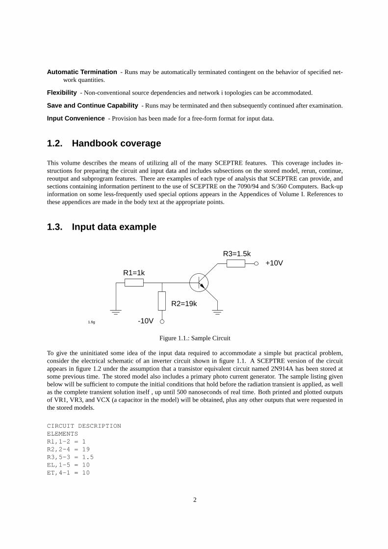
Figure 1.1.: Sample Circuit
To give the uninitiated some idea of the input data required to accommodate a simple but practical problem,consider the electrical schematic of an inverter circuit shown in figure 1.1. A SCEPTRE version of the circuitappears in figure 1.2 under the assumption that a transistor equivalent circuit named 2N914A has been stored atsome previous time. The stored model also includes a primary photo current generator. The sample listing givenbelow will be sufficient to compute the initial conditions that hold before the radiation transient is applied, as wellas the complete transient solution itself , up until 500 nanoseconds of real time. Both printed and plotted outputsof VR1, VR3, and VCX (a capacitor in the model) will be obtained, plus any other outputs that were requested inthe stored models.
CIRCUIT DESCRIPTIONELEMENTSRl,1-2 = 1R2,2-4 = 19R3,5-3 = 1.5EL,1-5 = 10ET,4-1 = 10
2

R1
10 V
T1
R3
R2 10 V
ET=
EL=
12.fig
2
53
4
Figure 1.2.: SCEPTRE Version
Tl,2-1-3 = MODEL 2N914A (PERM)OUTPUTSVR3, VR1, VCXT1, PLOTRUN CONTROLSSTOP TIME = 500, RUN INITIAL CONDITIONSEND
The detailed rules will be given throughout this manual for generating circuit descriptions such as the one above.
3
2. SCEPTRE use
The DC, transient or AC solutions of large electrical networks are computed on request when the circuit descriptionlanguage described herein is used to convey all the necessary information to the SCEPTRE program. The user isnot required to write the network equations or to possess a knowledge of computer programming. This Sectiondescribes the preparation of circuits and the circuit description language recognized by SCEPTRE.
2.1. Circuit preparation
The first step taken in using the SCEPTRE program is to prepare an equivalent circuit drawing of the circuit to beanalyzed. The equivalent circuit may consist of resistors, capacitors, inductors, mutual inductance, voltage sources,and current sources, and/or stored models containing these elements. All of these elements may be linear and/ornonlinear. Furthermore, most equivalent circuits composed of these elements can be accommodated. This allowsthe use of either standard or complex experimental equivalent circuits. The value, or behavior, of any equivalentcircuit element may be defined by a numerical constant, tabular list, or mathematical expression.
After the equivalent circuit has been drawn, each node is given an arbitrary alphanumeric designation consistingof six characters or less. A node is defined as the point of common potential (voltage) at the junction created bythe connection of two or more network elements.
Next, each component or element in the circuit is given a unique name consisting of not more than five alphanu-meric characters. The first character of each element name must be R, C, L, E, or J corresponding to the elementtype; i.e., resistor, capacitor, inductor, voltage source or current source, respectively. The letter M is used to des-ignate mutual inductance in the same way. The two exceptions to this are the circuit designation for a storedmodel (see subsection 2.3.1) which has no specific rule for its first character, but should be limited to a total ofthree alphanumeric characters, and the Convolution model (Appendix A.8), the first character of which is a K. Itis normally very helpful to record on the equivalent circuit diagram the names and nodes chosen. Current flowdirections and source polarities should also be indicated.
The circuit parameter values should be specified in a consistent set of parameter units. Although any consistentset is acceptable, the system given in table 2.1 is useful for high-speed transistorized circuits. If another systemis desired, the most effective choice is units of voltage, current and time that correspond to the magnitude ofthose that are expected in the problems; then determine units of R, L, and C from the fundamental current-voltagerelationships. This choice is always possible in a practical circuit, since the analyst should have some approximateidea of the range of variables.
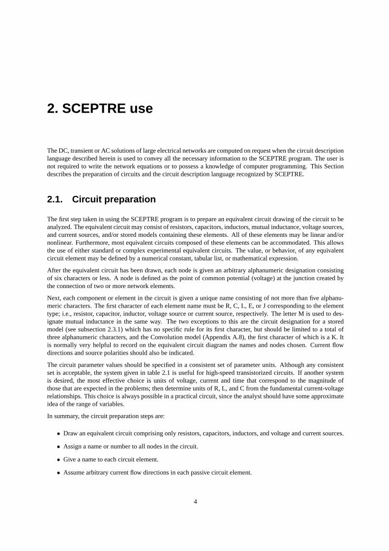
In summary, the circuit preparation steps are:
• Draw an equivalent circuit comprising only resistors, capacitors, inductors, and voltage and current sources.
• Assign a name or number to all nodes in the circuit.
• Give a name to each circuit element.
• Assume arbitrary current flow directions in each passive circuit element.
4
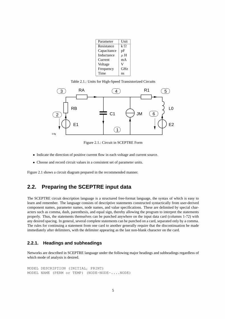
Parameter UnitResistance k ΩCapacitance pFInductance µ HCurrent mAVoltage VFrequency GHzTime ns
Table 2.1.: Units for High-Speed Transistorized Circuits
3.fig
RA
RBC1 JM
R1
L0
E2E11
2
3 4 5
6
Figure 2.1.: Circuit in SCEPTRE Form
• Indicate the direction of positive current flow in each voltage and current source.
• Choose and record circuit values in a consistent set of parameter units.
Figure 2.1 shows a circuit diagram prepared in the recommended manner.
2.2. Preparing the SCEPTRE input data
The SCEPTRE circuit description language is a structured free-format language, the syntax of which is easy tolearn and remember. The language consists of descriptive statements constructed syntactically from user-derivedcomponent names, parameter names, node names, and value specifications. These are delimited by special char-acters such as comma, dash, parenthesis, and equal sign, thereby allowing the program to interpret the statementsproperly. Thus, the statements themselves can be punched anywhere on the input data card (columns 1-72) withany desired spacing. In general, several complete statements can be punched on a card, separated only by a comma.The rules for continuing a statement from one card to another generally require that the discontinuation be madeimmediately after delimiters, with the delimiter appearing as the last non-blank character on the card.
2.2.1. Headings and subheadings
Networks are described in SCEPTRE language under the following major headings and subheadings regardless ofwhich mode of analysis is desired.
MODEL DESCRIPTION (INITIAL, PRINT)MODEL NAME (PERM or TEMP) (NODE-NODE-....NODE)
5

(Comment or message cards, if any, up to 11 allowed)ELEMENTSDEFINED PARAMETERSOUTPUTSFUNCTIONSINITIAL CONDITIONSCIRCUIT DESCRIPTION(Comment or message cards, if any, up to 11 allowed)ELEMENTSDEFINED PARAMETERSOUTPUTSINITIAL CONDITIONSFUNCTIONSRUN CONTROLSSENSITIVITYMONTE CARLOWORST-CASEOPTIMIZATIONRERUN DESCRIPTION (N)(Comment or message cards, if any, up to 11 allowed)ELEMENTSDEFINED PARAMETERSINITIAL CONDITIONSFUNCTIONSRUN CONTROLSCONTINUERUN CONTROLSRE-OUTPUTOUTPUTS (required) S/360 onlyRUN CONTROLS (optional)(In the IBM 7090/94 version, no subheadings are permitted under thisheading.)END
The MODEL DESCRIPTION heading is used when it is desired to store one or more models. The MODEL namecard, comment cards (optional), and any or all of the five subheadings listed can be used for each model for eitherpermanent or temporary storage under the MODEL DESCRIPTION heading. One or more models may be enteredunder one MODEL DESCRIPTION heading.
The CIRCUIT DESCRIPTION heading is always used when any network is presented for analysis. Any or all ofthe ten subheadings listed under the heading may be used.
The RERUN DESCRIPTION heading is used whenever the rerun feature is exercised. All changes to the masternetwork must appear under this card. Any or all of the five subheadings listed under this heading may be used.
The CONTINUE heading is intended for use only when continued computation is desired after a problem has beenoriginally run. The only subheading permitted under this heading is RUN CONTROLS. The only other headingthat may appear together with CONTINUE in a run is END.
The RE-OUTPUT heading is used whenever the user desires output from a previously completed run withoutrepeating that run. No subheadings are permitted under this heading on the 7090/94. The only other heading thatmay appear with RE-OUTPUT on the 7090/94 is END. On the S/360, the OUTPUT subheading is required andthe RUN CONTROLS subheading may be used (see subsection 2.6).
6

The END heading is used to terminate every input data deck submitted to SCEPTRE. This heading is the only onethat must always be used without subheadings.
The data supplied within each of the subheadings consists of descriptive statements which are constructed asproperly punctuated sequences of symbols. The group heading, subheading and subsequent statements may bepunched on a card with arbitrary spacing or location from columns 1 to 72. During a single run the user cannot useall six major headings, although all ten subheadings under CIRCUIT DESCRIPTION could well be used.
Unique sequences of symbols and punctuation are used to convey information in each of the subheadings. Adefinition of each of the symbols in the subheadings follows:
Element Name - Denotes the name given to each component (including model circuit designations) of a circuit(e.g., RA, LLX, E17). No more than five alphanumeric characters may be used to name an element. Modelcircuit designations are limited to no more than four alphanumeric characters.
Node - Denotes the designation assigned to each node of a circuit. No more than six alphanumeric charactersmay be used to name a node.
Number - A numerical constant that may be written as a signed quantity in either integer or decimal form andwith or without an exponent. Up to 13 characters may be used to represent a number. For example, numbersmay be written in the following forms: 10, 10., 10.0, -.1, -0.1, +1.4, 6.4E9, -74.3E-7, 7E+11, -176.6667E5.
Constant - Same as Number, except a decimal point must be included in the specification of the numericalconstant.
Value - Will be used to denote any of the following: Number, Defined parameter, TABLE, EQUATION, EX-PRESSION, or External Function.
Special Value - Will be used to denote any of the following: Value, Constant*Resistor Current, Constant*ResistorVoltage, Value*Current Source, DIODE TABLE, or DIODE EQUATION (X1, X2).
Variable - Denotes any of the following:
• The voltage or current associated with any element as VR1, VJ7, IE4, ILM, etc.
• Any source or source derivative as J17, DJ17, E4, DE4, etc.
• Any defined parameters as P7, DP7, etc.
• Any element value as R17, CA, M12, etc.
• Time as TIME.
• Frequency as FREQ.
• Any internal parameter (see subsection 2.2.11).
V Element Name or I Element Name - Denotes the element voltage or current of ELEMENT NAME. For ex-ample, the voltage across capacitor CAB1 would be referred to as VCAB1, and the current through inductorLCHOK would be referred to by ILCHOK.
TABLE Name (Independent Variable) - Used when a variable circuit quantity is given in tabular form. Thetable used must be given a unique name prefixed by TABLE or simply T, and followed by a single indepen-dent variable in parenthesis. The name may consist of up to five alphanumeric characters. The independentvariable may be any of the quantities defined under VARIABLE, such as TABLE 1A (VC1). If an indepen-dent variable, including the enclosing parenthesis is not supplied, then TIME will automatically be chosen.
EQUATION Name (Argument List) - Used when a variable circuit quantity is given in closed form. The equa-tion must be given a name prefixed by EQUATION or simply Q and followed by one or more argumentsseparated by commas and enclosed in a parenthesis. The EQUATION name may consist of up to five al-phanumeric characters. The argument list may consist of any VARIABLE, CONSTANT, and TABLE (andits independent variable). For example,EQUATION 39 (VCX, J2, TIME, TABLE 2 (VC7)).
7

EXPRESSION Name (Math Definition) - This form is an alternative to EQUATION entry that may be usedto describe a variable quantity. It is somewhat more complex than the EQUATION form, but it has the virtueof needing no further description under FUNCTIONS. The expression must be given a name prefixed byEXPRESSION or simply X and followed by the mathematical definition. The EXPRESSION name mayconsist of up to five alphanumeric characters. It is suggested that numerical designation be used to avoid anypossible confusion with some internal parameters. For example,X14 (10. * SIN (.628 * TIME)).
Any equation for table must be defined more completely under FUNCTIONS. More detail is given in subsections2.2.2 and 2.2.6.
The input data deck describing a network is formed simply by punching the heading card and the associated datasequence for each of the defined data groups.
Remarks such as title, user name, and date may be supplied for output identification purposes by punching thedesired remarks on cards following the CIRCUIT DESCRIPTION card and preceding the first subheading card.The number of comment cards must not exceed 11, and the entire remark will appear as the title of the outputlisting and plots.
The sequence for each of the subheadings in terms of the symbols defined previously are subsequently detailed.
2.2.2. Elements
This subsection covers the formats required for entering element data into SCEPTRE. The general discussionpertaining to all elements is followed by four subsections discussing special conditions which pertain to certainelement entries. These subsections cover mutual inductance (subsection 2.2.2), source derivatives (subsection2.2.2), elements with bounds (subsection 2.2.2), and AC (complex) sources (subsection 2.2.2).
All elements (resistances, capacitances, inductances including mutual, voltage and current sources, source deriva-tives and model circuit designations) that are to be component parts of the network under analysis must be in-troduced under this subheading. Entries allowed under the elements subheading are summarized in table 2.2.Although any combination of alphanumeric characters (maximum 4) can be used for model circuit designations,names unique from other element names are recommended. Alphanumeric character lengths are listed in table2.10, subsection 2.2.9. The general form for entries under the ELEMENTS subheading is:
element name, node-node = value
Each network element is defined by stating the element name, the nodes between which the branch is connected,and the component value. The connection nodes are specified in a from-to order corresponding to the assumeddirection of current flow. The actual tabular values or analytical expressions of elements that are implicitly definedas variables are specified in subsection 2.2.6. More than one element may be described on a card if the elementsare separated by commas.
Some examples that illustrate proper entries under elements for the constant valued elements of the network offigure 2.1 are:
E1, 1-2 = 20E2, 1-6 = 20JM, 1-4 = 2E1
Note that any of these constant elements may be entered with or without decimal points, or by use of the E format.Note also that the proper reference direction for voltage sources p p correspond to the direction of current orpositive charge movement within the voltage source.
NOTES to Table 2.2:
8
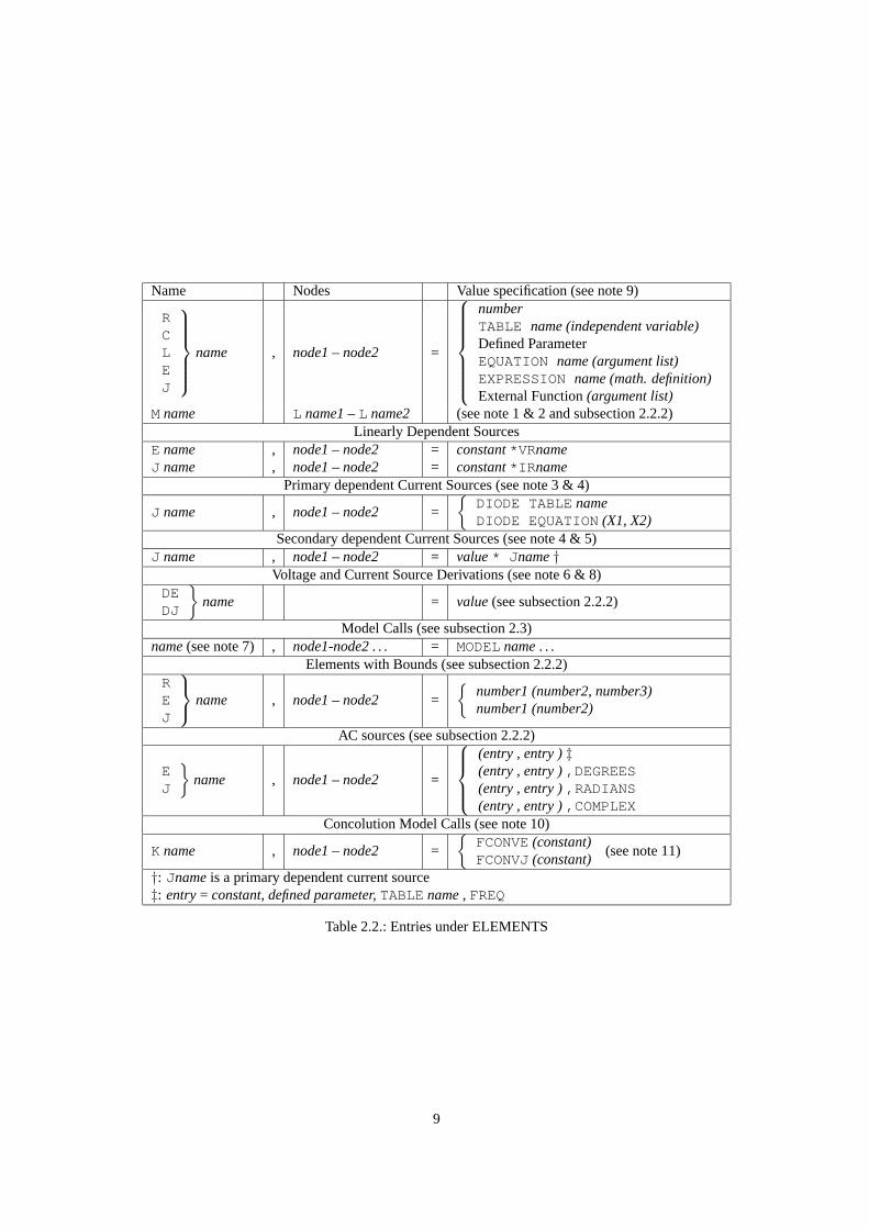
Name Nodes Value specification (see note 9)
RCLEJ
name , node1– node2 =
numberTABLE name (independent variable)Defined ParameterEQUATION name (argument list)EXPRESSIONname (math. definition)External Function(argument list)
Mname L name1– L name2 (see note 1 & 2 and subsection 2.2.2)Linearly Dependent Sources
E name , node1– node2 = constant*VRnameJ name , node1– node2 = constant*IR name
Primary dependent Current Sources (see note 3 & 4)
J name , node1– node2 =
DIODE TABLEnameDIODE EQUATION(X1, X2)
Secondary dependent Current Sources (see note 4 & 5)J name , node1– node2 = value* J name†
Voltage and Current Source Derivations (see note 6 & 8)DEDJ
name = value(see subsection 2.2.2)
Model Calls (see subsection 2.3)name(see note 7) , node1-node2 . . . = MODELname. . .
Elements with Bounds (see subsection 2.2.2)REJ
name , node1– node2 =
number1 (number2, number3)number1 (number2)
AC sources (see subsection 2.2.2)
EJ
name , node1– node2 =
(entry , entry )‡(entry , entry ),DEGREES(entry , entry ),RADIANS(entry , entry ),COMPLEX
Concolution Model Calls (see note 10)
K name , node1– node2 =
FCONVE(constant)FCONVJ(constant)
(see note 11)
†: Jnameis a primary dependent current source‡: entry= constant, defined parameter,TABLEname, FREQ
Table 2.2.: Entries under ELEMENTS
9

1. All C,R,L and M entries will be treated as REAL*8 constants in the AC calculations. Before making the ACcalculations, SCEPTRE will evaluate any entries which are given as functions. For example, a capacitor maybe a function of voltage and a resistor may be a function of time. SCEPTRE will evaluate these functions atTIME=0, using supplied or calculated initial conditions. The appropriate values so obtained will be used inthe AC calculations. Elements as a function of frequency are not permitted in AC calculations.
2. All voltage and current sources which are given as constants (DC sources) or as functions of TIME (Transientsources) will be given a value of zero in AC calculations, and a WARNING message will be printed outwhenever the argument TIME is used.
3. In order to obtain an AC analysis around a circuit’s DC operating points, the user must either supply InitialConditions (see paragraph 2.2.5), or must enter RUN INITIAL CONDITIONS under the RUN CONTROLSsubheading of CIRCUIT DESCRIPTION. If initial condition are supplied, then SCEPTRE determines allelement values dependent on these DC voltages and currents.
4. Primary and secondary dependent current source specifications may be used to represent certain semicon-ductor junctions when requesting Initial Conditions solutions.
5. By Definition this class of current source can appear only if the appropriate diode source has previously beenincluded. The secondary source must be specified only as a value times the primary source.
6. Although this entry is permitted in AC calculations, a time-source, and hence its derivatives, are not mean-ingful. The source will be treated as in Note 2 above and the derivatives ignored.
7. Model circuit designation names can be any combination of no more than four alphanumeric characters.Names unique from other element names are recommended.
8. If the topology of the circuit dictates that a time derivative is required for a transient analysis (e.g., capacitorand independent voltage source loop, or inductor and independent current source cut set), then the same istrue for an AC analysis. However, for AC no card entry is required. A time derivative of an AC source meanssimply a multiplication by jω. SCEPTRE will detect this situation and will automatically handle it.
9. A complex defined parameter, W, cannot be used as a value specification.
10. Convolution models are either series combination of voltage source and resistor (FCONVE) or parallelcombination of current source and resistor (FCONVJ). See Appendix A.8.
11. The constants in the Convolution Model Call are arbitrarily assigned integers identifying the impedance oradmittance functions stored on Disk 12 as explained in Appendix A.8.
Examples of variable element entries using EQUATION, TABLE or EXPRESSION descriptions are as follows:
El, 1-2 = TABLE 3 (TIME)E2, 1-6 = EQUATION 47 (VC1, TABLE 2 (ILO),36.)JM, 1-4 = EQUATION 47 (VC1, P5, 15.)RA, 3-4 = TABLE 5 (TIME)LZ, 1-5 = EXPRESSION 7 (10. *ILZ + 20.)
The tabular entries for TABLE 3 and TABLE 5, as well as the analytical expression for EQUATION 47 mustbe entered under the FUNCTIONS subheading (subsection 2.2.6). A good general rule to follow throughout theprogram is that all constants inside parentheses must include decimal points. A more convenient form that alwaysmay be used is to replace the word EQUATION by Q, the word TABLE by T, and the word EXPRESSION by X.
El, 1-2 = T3(TIME)JM, 1-4 = Q47 (VC 1, P5, 15.)LZ, 1-5 = 47 (10.*ILZ + 20.)
10
The second and third designations in the SPECIAL VALUE list are intended to accommodate the class of linearlydependent sources that are encountered in small signal transistor equivalent circuits (see subsection 3.3). Thefourth designation was designed for the class of secondary dependent current sources that always appear in thelarge signal Ebers-Moll transistor equivalent circuit (see subsection 3.2). The capability of specially processingthese sources has been built into the program and should always be entered directly in the ELEMENTS sectionwithout parentheses. Examples of these appear in this subsection.
The last two designations in the SPECIAL VALUE list are reserved for primary dependent current sources thatrepresent diodes or transistor junctions. DIODE EQUATION (X1, X2) would be used when any diode or tran-sistor junction has been entered, and the user wishes to employ the conventional closed form representation(J = Is(eΘV J − 1)). The value of X1 must correspond toIs in the diode equation, and the value of X2 mustcorrespond toΘ. The program will automatically use the voltage across that particular current generator as theindependent variable, and for that reason this voltage need not be specified. If for example, a current generator thatis named J18 and is connected between nodes 1 and ground is to be described by the conventional diode equationas1 · 10−7(e30V J − 1), the appropriate entry would be
J18, 1 - GND = DIODE EQUATION (1.E-7, 30.)
Note that decimal points are required for the constants 1 and 30. No further description is required under FUNC-TIONS. The designation DIODE TABLE N is used when any diode or transistor junction is to be represented intabular form. The independent variable will automatically be taken as the voltage across the current generator.Therefore, the required entry is simply
J18, 10 - 3 = DIODE TABLE 1
The tabular entries for DIODE TABLE 1 must be entered under the FUNCTIONS subheadings (subsection 2.2.6).
Examples of typical component descriptions that appear in the ELEMENTS group are shown below:
R7, 4-5 = 11.5, E1, GND-1 = 6JA, 0-4 = .98 * J18E12, C-7 = .0005 * VRC
JA is a secondary dependent current source. JK and E12 are linearly dependent sources.
LX3, 9-3 = EQUATION 15X (ILX3,TIME)Tll, 2-3-7 - MODEL 2N7479AA
Reference to the FUNCTIONS section (Section 2.2.6) is never required for a given entry when the expressionformat is used. The rules for the mathematical definition become specialized only in the case when a table is to beused as an argument. For example, if it is desired to enter capacitor C1 as 10 + 80 * (TABLE 7), where TABLE 7is a function of VC1, an appropriate entry would be
C1, 7-8 = X314 (10. +80. * XTABLE (T7, VC1))
Note that in this special case the word TABLE is preceded by X and that both the table name, in this case T7, andthe independent variable of the table VC1, must be included in parentheses. Decimal points must always be givenwith all constants used in an EXPRESSION. This same entry is given in equation form in subsection 2.2.6.
11

4.fig
L1
L2
L3
I3
I2
I1
MutualInductance
M12M13M23
sign
+-
-
Figure 2.2.: Mutual Inductance Polarities
Mutual Inductance
Mutual inductance is entered according to the general format:
Mname, Lname-Lname = value
If coupling exists between inductors L1 and L2, the appropriate entry must include these elements in place of thenode identification as
MX, L1-L2 = TABLE 1 (IL1)
or
MX, L1-L2 = 32.4
In addition, a physical limitation of the principle of mutual inductance must be observed in order to have a physi-cally realizable circuit. That is, since coefficient of coupling,k, is always less than unity and by definition
k =M√L1L2
< 1
the user should be certain thatM <√L1L2. Stated in words, the mutual inductance between any two inductors
must be less than the square root of the product of the self-inductances of the components between which themutual inductance exists. The sign of M is positive if in a given winding the induced voltage of mutual inductanceacts in the same direction as the induced voltage of self-inductance. If the induced voltage of mutual inductanceopposes the induced voltage of self-inductance in a given winding, M is negative. The proper sign for M for theassumed current directions is illustrated in figure 2.2.
Source Derivatives
The time derivatives of sources must be supplied as input data when certain network configurations are encoun-tered1. These situations occur whenever a variable voltage source is connected in a loop containing only capacitorsand other voltage sources, and whenever a variable current source is connected in a cut set containing only induc-tors and other current sources (see figure 2.3).
If the sources in question are constant, the zero derivative will automatically be supplied and the user need not beconcerned. If the user fails to supply a source derivative when one is required, the run will be terminated with anappropriate diagnostic message. The general form for a source derivative entry is
1Except for AC Analysis. See Table 2.2, note 8
12

C1
J1
5.fig
E7C3 C2
L1
L3
L2
Source LoopCapacitor-Voltage Inductor-Current Source Cut Set
Figure 2.3.: Configurations That Require Source Derivatives
DEname = valueDJname = value
where the name is that of the appropriate E or J source. An example would be
DERIVATIVE E7 = TABLE 2
or more simply
DE7 = TABLE 2
Elements with Bounds
Three of the DC options, Monte Carlo, Worst-Case, and Optimization require additional information in the entriesunder ELEMENTS. For a Monte Carlo calculation, it is necessary to specify parameters for distribution of thevariable elements. For Worst-Case and Optimization calculations, minimum and maximum values of the indepen-dent variables must be specified. In all cases, the element information is provided by bounds added in parenthesesafter the element values. Except as noted at the end of this paragraph bounds are provided by statements, underELEMENTS, of the form
element name, none-node = number (number,number)
or
element name, node-node = number(number)
The first form gives two numbers in parentheses. SCEPTRE reads the smaller number as the lower bound and thelarger as the upper bound. The second form has one number in parentheses. In this form, SCEPTRE reads thenumber as the percentage variation allowed in the nominal value of the elements. Examples might be
R2, NZ-N5=12(11,13)
and
R1, N1-NB=6(10)
13

The first example specifies the nominal value of R2 as 12, with lower and upper bounds of 11 and 13, respectively.The second example specifies that the value of R1 is 6±10%.
For Worst-Case and Optimization, the lower and upper bounds are taken to be the limiting values for the element.For these calculations, the nominal value must lie within these limits.
For Monte Carlo calculations, the element distribution mean and standard deviation are computed from the lowerand upper bounds as:
mean=upper bound+ lower bound
2
standard deviation=upper bound− lower bound
6
The exception, mentioned above, to the use of numbers exclusively in specifying elements with bounds is asfollows: Examples with bounds may be specified as values or diode equations if the values or diode equationsare expressed in terms of defined parameters with bounds under DEFINED PARAMETERS. Subsection 2.2.3describes the allowable format for defined parameters with bounds. An example of an entry under ELEMENTS is
R3, N12-N10=X3(P3+P4)
AC Sources
Source voltages and currents for AC calculations are complex numbers and, therefore, require both real and imag-inary parts (or magnitude and phase) for their definition. The format for entering an AC source is:
Ename, node-node = (entry, entry), type
for a voltage source and
Jname, node-node = (entry, entry), type
for a current source. The word entered for ’type’ identifies the meaning of the two entries in the parentheses.’Type’ may be either DEGREES, RADIANS or COMPLEX. If DEGREES or RADIANS is entered, the first entryin parentheses is the magnitude, in the polar coordinate expression of the voltage (or current), and the second entryis phase angle. If type is specified as COMPLEX, the first entry in the parentheses is the real portion of the complexexpression in cartesian coordinates, and the second entry is the imaginary portion. ’Type’ need not be specified. Ifit is not, the default value is DEGREES.
An entry, as described above, may be any of the following: constant, the problem frequency (denoted by FREQ),a TABLE name (where the independent variables must be stated because the default value of the independentvariable is TIME, and the AC calculation takes time as zero), or a real defined Parameter.
The maximum allowed number of independent AC sources is fifty. The maximum number allowed for linearlydependent AC sources plus secondary dependent AC current sources is also fifty.
The following are examples of AC source definitions:
E1, N1-M3 = (12., 4.), COMPLEX
means that voltage source E1, between nodes N1 and M3, is expressed in complex form as 12+4j volts.
J7, N4-N7 = (T1(FREQ), P6), RADIANS
means that current J7, between nodes N4 and N7, is expressed in polar coordinates, where the magnitude is afunction of frequency to be obtained from Table 1 and the phase angle, in radians, is as specified by P6 underDEFINED PARAMETERS.
14

2.2.3. Defined parameters
Any variable that can be described in terms of any network variable and/ or any Number may be defined, and thisquantity may be used as an ELEMENT value, an argument in an equation or table, or an output at each time stepof the problem, in the same manner as any conventional output. Examples of the use of this feature are given inSection 4. More than one defined parameter may be entered on a card if they are separated by commas.
Real Valued Defined Parameters
The input format for real-valued defined parameters requires that the first letter be P followed by no more than fivealphanumeric characters. The general form for entries under DEFINED PARAMETER IS:
Pname = value
Some possible combinations are:
PWR = EXPRESSION 69 (IE 3 * E3)P2 = TABLE 1 (VC7)PX7 = EQUATION 2 (VC7, VR1)
For the special case in which the derivative of a quantity is supplied, the first two letters must be DP followed byno more than four alphanumeric characters, or in general
DPxxxx = value
Real-Valued Defined Parameters with Bounds
Real-valued defined parameters with bounds may be used as independent variables in DC calculations (under theMONTE CARLO, WORST-CASE or OPTIMIZATION subheadings of CIRCUIT DESCRIPTION, see subsection2.2.8). When independent variables are used in this manner, they must be specified with bounds under DEFINEDPARAMETERS. The format is:
Pname = number (number, number)
or
Pname = number (number)
The first form gives two numbers in parentheses. SCEPTRE reads the smaller number as the lower bound and thelarger as the upper bound. The second form has one number in parentheses. In this form, SCEPTRE reads thenumber as the percentage variation allowed in the nominal value of the independent variable.
For Worst-Case and Optimization calculations, the nominal value must not lie outside of the region defined by theupper and lower bound.
15
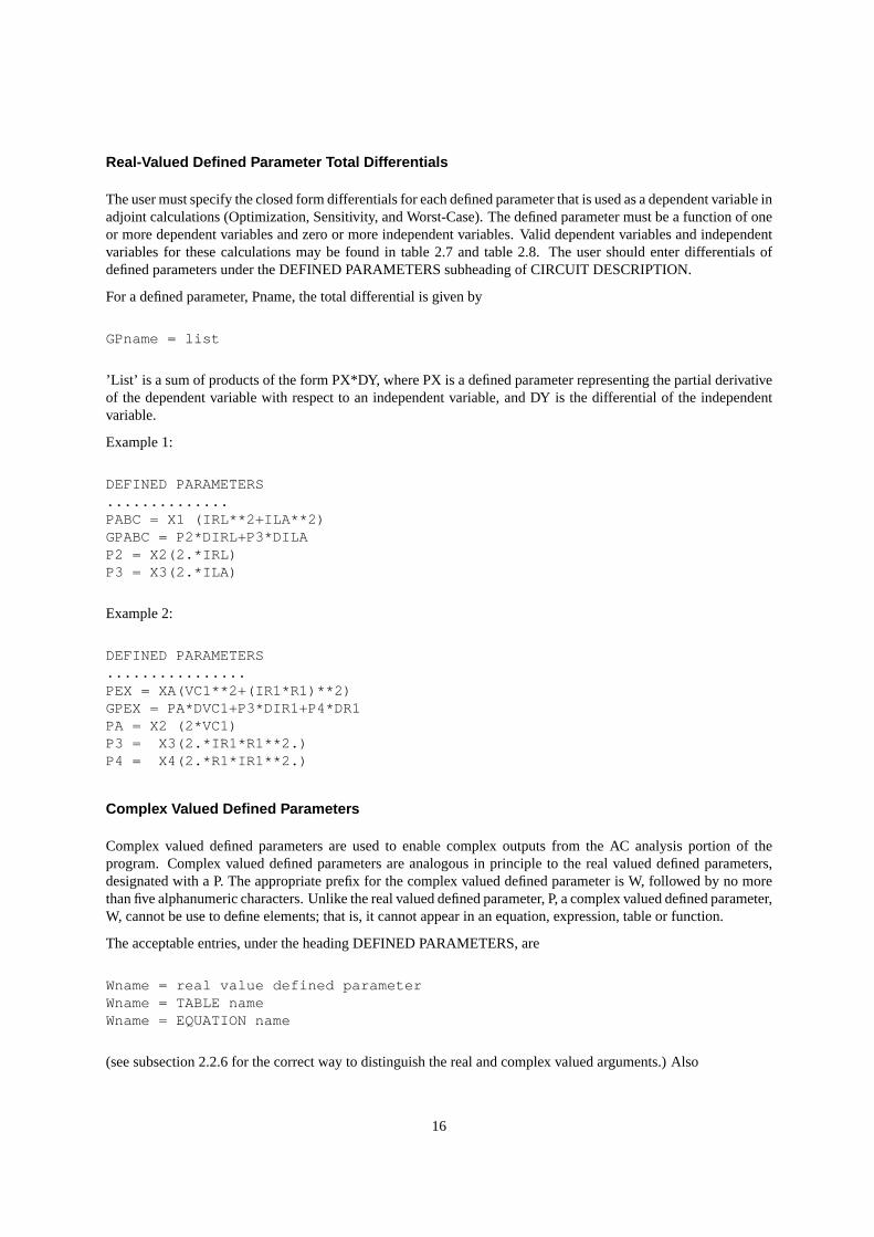
Real-Valued Defined Parameter Total Differentials
The user must specify the closed form differentials for each defined parameter that is used as a dependent variable inadjoint calculations (Optimization, Sensitivity, and Worst-Case). The defined parameter must be a function of oneor more dependent variables and zero or more independent variables. Valid dependent variables and independentvariables for these calculations may be found in table 2.7 and table 2.8. The user should enter differentials ofdefined parameters under the DEFINED PARAMETERS subheading of CIRCUIT DESCRIPTION.
For a defined parameter, Pname, the total differential is given by
GPname = list
’List’ is a sum of products of the form PX*DY, where PX is a defined parameter representing the partial derivativeof the dependent variable with respect to an independent variable, and DY is the differential of the independentvariable.
Example 1:
DEFINED PARAMETERS..............PABC = X1 (IRL**2+ILA**2)GPABC = P2*DIRL+P3*DILAP2 = X2(2.*IRL)P3 = X3(2.*ILA)
Example 2:
DEFINED PARAMETERS................PEX = XA(VC1**2+(IR1*R1)**2)GPEX = PA*DVC1+P3*DIR1+P4*DR1PA = X2 (2*VC1)P3 = X3(2.*IR1*R1**2.)P4 = X4(2.*R1*IR1**2.)
Complex Valued Defined Parameters
Complex valued defined parameters are used to enable complex outputs from the AC analysis portion of theprogram. Complex valued defined parameters are analogous in principle to the real valued defined parameters,designated with a P. The appropriate prefix for the complex valued defined parameter is W, followed by no morethan five alphanumeric characters. Unlike the real valued defined parameter, P, a complex valued defined parameter,W, cannot be use to define elements; that is, it cannot appear in an equation, expression, table or function.
The acceptable entries, under the heading DEFINED PARAMETERS, are
Wname = real value defined parameterWname = TABLE nameWname = EQUATION name
(see subsection 2.2.6 for the correct way to distinguish the real and complex valued arguments.) Also
16

Wname = EXPRESSION name
(see subsection 2.2.6 for a list of the more general FORTRAN complex operational functions available.) Also
Wname = external function
(It is the user’s responsibility, when writing FORTRAN programs, to insure the correct declaration and usage ofcomplex valued quantities.)
Alternatively, the format allowed for specifying AC sources can be used. This format is
Wname = (entry, entry) type
where the details are described in subsection 2.2.2.
2.2.4. Outputs
Tabular Form
Any output must consist of some dependent variable which is a function of some independent variable. SCEPTREoutputs consist of printed tabular listings of requested dependent variables as functions of time and/or plots of thedependent variables as functions of time or some other independent variable. In SCEPTRE, the following generalquantities may serve as either dependent or independent variables:
• The voltage or current associated with any passive element as VR1, IL6.
• The voltage or current associated with any source as E1, IE1, J2, VJ2.
• Any element value as C17.
• Any transient state variable derivative as DC4, DL13B.
• Any Defined Parameter as P12.
• Any Complex Valued Defined Parameter (Wname) in AC Calculations.
• Any Defined Parameter derivative as DP12 if the user has supplied one.
• Any internal parameter as defined in table 2.11.
All requested outputs in SCEPTRE will be supplied in printed tabular form. The general format for requestingprinted outputs is:
variable, variable, variable
and/or
variablevariablevariable
Note that no output request card ever ends with a comma.
17

Plotted Form
In addition, the user has the option of requesting plotted outputs for any or all quantities. If plotted outputs aredesired, the word PLOT is used as the last entry on each output request card for which plots are desired. Thegeneral format is:
variable, variable, PLOT
and/or
variable, PLOTvariable, PLOT
Some typical output requests follow:
VR3, IR3, VR2VR5, VC29VRY, VC1, ESUP, PLOTIC8
Note that more than one output can be requested on a single card. The third card indicates that three quantities arerequired and that all three are to be plotted as well as printed. The quantity, IC8, (the current through capacitor C8)would be output in printed form only. If the word PLOT is used, no other dependent variable may follow it on thatcard.
All indicated variables in the above example will use time as the independent variable. If a different independentvariable is desired for the plotted form, the following format must be used.
IC14, PLOT (VC14)
In this case, the current through capacitor C14 would be plotted as a function of the voltage across it. The printedoutput would be IC14 as a function of time.
Additional flexibility is available to permit the user to attach a different label to any output quantity except TIME.Consider that elements C1 and R7 exist in a given network and that the voltage across both (VC1 and VR7) are ofinterest. If the user decides to rename them as VIN and VOUT, the outputs may be requested as VC1 (VIN), VR7(VOUT), PLOT. All renames must be limited to six alphanumeric characters and the first character may be anyalphanumeric character. The plot, rename, and choice of independent variable options can be presented in termsof the general format as:
yqty(ylabel),......, PLOT(xqty(xlabel))
If no rename is desired, the general format reduces to
yqty, ......, PLOT (xqty)
If, in addition, only time is desired as the independent variable, this can be further reduced to
yqty,........, PLOT
And, if no plotted information is desired, the simplest form arises as
yqty, ....
18

Composite Plots
A specialized plot format is available in which up to nine dependent variables may be plotted against a commonabscissa. The ordinate for each dependent variable runs across the page and is separately scaled, and uniquegraphic characters are used to represent each quantity. Use of this feature requires that all of the quantities whichare to be plotted together may be requested on the same card or sequence of cards under OUTPUTS followed by aspecific plot name. For example,
OUTPUTSVC1, VC2,P13, PLOTVR11, VCET1, JET6, IE4, PLOT 1
In this case, quantities VC1, VC2 and P13 would be plotted singly, as usual. Quantities VR11, VCET1, JET6, andIE4 would be plotted together, since they have been requested together with a plot that has been ’named’ simplyas 1. Any plot name may include up to six alphanumeric characters and more than one name may be used to plotdifferent combinations of quantities.
The composite plot feature also requires a PLOT INTERVAL entry under RUN CONTROLS. While this is a RUNCONTROL entry, it is discussed here because it relates only to composite plots, and its omission will cause therequested plots to appear in their usual separate formats.
The physical length of any composite plot may be controlled. The number of pages encompassed by the abscissa(independent variable) is determined by the problem duration (STOP TIME) and a user supplied entry calledPLOT INTERVAL. The former divided by the latter will determine the number of lines required which will, inturn, determine the number of pages required. For the system S/360, 66 lines will fill one page. Therefore, aproblem duration of 1000 and a PLOT INTERVAL of 5 will require 1000/5 = 200 lines, or three pages, plus twolines on a fourth page (plus approximately three lines per variable for identification and scaling information). ThePLOT INTERVAL entry always appears under RUN CONTROLS, and the format is simply:
PLOT INTERVAL = number
Only one PLOT INTERVAL will be recognized regardless of the number of composite plots that are requested.For additional discussion of composite plots, see Appendix A.5.
Convolution Outputs
The above discussion about outputs also applies to transient runs employing the Convolution option. One precau-tion is noted here. When the user requests an element of a Convolution model as output, he must prefix its nameKname (see table 2.2) with a letter denoting the element desired. The code is as follows:
E for the voltage source of an impedance kernel; e.g., EKname
J for the current source of an admittance kernel; e.g., JKame
R for the resistance value of a kernel; e.g.. RKname
Additional prefixes, I and V, are required if the user is requesting currents and voltages of these elements; e.g.,IEKname, IRKname, VJKname, VRKname. See subsection 4.6 for a discussion of Convolution kernels.
19
AC Outputs
The results of AC calculations can be obtained as outputs in either tabular or plotted form. The general rules foroutput requests given in subsections 2.2.4 and 2.2.4 apply equally to AC outputs, except that AC outputs are notgiven as functions of time. All AC tabular outputs and all but one type of plot are given as functions of frequency.The Nyquist plot gives the imaginary part of a complex function vs. the real part.
The standard forms of requests, under OUTPUTS,
variable, variable, variable
and/or
variablevariablevariable
will produce a tabular printout of magnitude vs. frequency, and phase in degrees vs. frequency for each variable.This is the default entry. The word DEGREES is optional. If the output is desired in radians, the proper entry is
variable, variable, RADIANS
The entry
variable, COMPLEX
produces a printout of the real part of each variable vs. frequency and the imaginary part vs. frequency.
If the word PLOT is added to the entry
Variable, COMPLEX, PLOT
a plot of the same data is also obtained, as described in subsection 2.2.4.
The Nyquist plot shows the imaginary part vs. the real part for each variable. The proper entry for the Nyquist plotis
variable, variable, NYQUIST, PLOT
In this entry only the word PLOT is optional. Both the plot and the printout will appear if the word NYQUISTappears in the entry.
2.2.5. Initial Conditions
The complete solution of the general transient analysis problem requires that all independent initial conditions besupplied. The set of all capacitor voltages and inductor currents that exist at the start of the problem are sufficientfor this purpose. These may be supplied by the user or computed by the program.
20
6.fig
7 8
L5 C11+ -
54
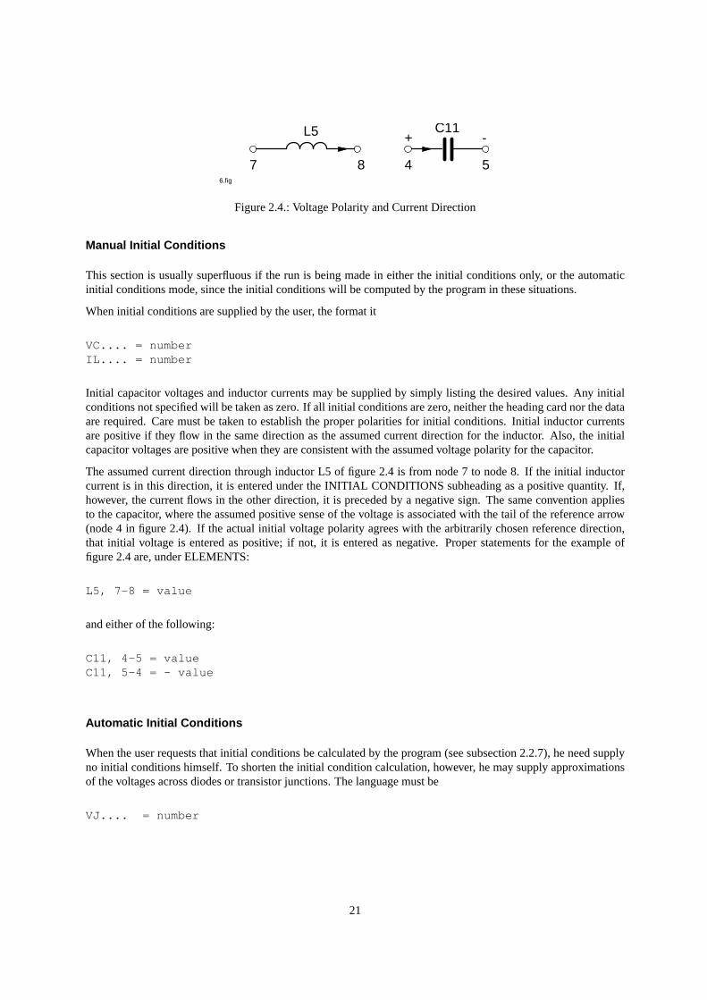
Figure 2.4.: Voltage Polarity and Current Direction
Manual Initial Conditions
This section is usually superfluous if the run is being made in either the initial conditions only, or the automaticinitial conditions mode, since the initial conditions will be computed by the program in these situations.
When initial conditions are supplied by the user, the format it
VC.... = numberIL.... = number
Initial capacitor voltages and inductor currents may be supplied by simply listing the desired values. Any initialconditions not specified will be taken as zero. If all initial conditions are zero, neither the heading card nor the dataare required. Care must be taken to establish the proper polarities for initial conditions. Initial inductor currentsare positive if they flow in the same direction as the assumed current direction for the inductor. Also, the initialcapacitor voltages are positive when they are consistent with the assumed voltage polarity for the capacitor.
The assumed current direction through inductor L5 of figure 2.4 is from node 7 to node 8. If the initial inductorcurrent is in this direction, it is entered under the INITIAL CONDITIONS subheading as a positive quantity. If,however, the current flows in the other direction, it is preceded by a negative sign. The same convention appliesto the capacitor, where the assumed positive sense of the voltage is associated with the tail of the reference arrow(node 4 in figure 2.4). If the actual initial voltage polarity agrees with the arbitrarily chosen reference direction,that initial voltage is entered as positive; if not, it is entered as negative. Proper statements for the example offigure 2.4 are, under ELEMENTS:
L5, 7-8 = value
and either of the following:
C11, 4-5 = valueC11, 5-4 = - value
Automatic Initial Conditions
When the user requests that initial conditions be calculated by the program (see subsection 2.2.7), he need supplyno initial conditions himself. To shorten the initial condition calculation, however, he may supply approximationsof the voltages across diodes or transistor junctions. The language must be
VJ.... = number
21

The iterative process will begin with any VJ.... entries that are supplied. One practical application of this typeof input would be to bias the ON and OFF sides of symmetric circuits such as flip-flops in the desired state.Approximate values could be supplied and the DC solution would then provide the correct voltages for the desiredstate. The results of the DC solution would then carry over to the beginning of the transient solution if one is calledfor. Appendix A.3 discusses special options in initial conditions.
NOTE: If the user requests automatic initial conditions for a transient run, and also supplies initial conditions forcapacitor voltages and inductor currents per subsection 2.2.5, his supplied values can appear as impulses at thestart of the transient run. This situation can lead to erroneous results. See [2, subsection 2.4.1].
2.2.6. Functions
In this data group, each of the tables and equations referred to under ’ELEMENTS’ and ’DEFINED PARAM-ETERS’ (subsections 2.2.2 and 2.2.3, respectively) must be defined in detail. If no such references have beenmade, neither the FUNCTIONS heading card nor data need be supplied. The equation definition sequence will bediscussed first.
Equation Definition Sequence
Each unique equation (used to define the variation of an element or defined parameter) is defined by giving theequation name, a dummy variable list, and the mathematical definition. The general format is
EQUATION name (Dummy Variable List) = (Mathematical Definition)
or
Q name (Dummy Variable List) = (Mathematical Definition)
The dummy variable list must contain the same number of entries as does the argument list in the original equationreference. Each dummy variable may contain up to six alphanumeric characters, the first of which must not be anumber or the letters I through N inclusive. For example, if an equation has been referenced under ELEMENTSas:
LX3, 9-3 = EQUATION 15X (ILX3, TIME, VC1)
then this equation could be explicitly defined under FUNCTIONS as:
EQUATION 15X (A, B, C) = (Mathematical Definition)
or
Q 15X (A, B, C) = (Mathematical Definition)
The dummy variables in this case are A, B, C which replace ILX3, TIME and VC1, respectively. The mathematicaldefinition itself must be included in parenthesis and must be written in terms of A, B, C, along with any constantsand allowable subprogram functions that apply. It is important to mention that there would be no need for the userto reserve quantities A, B, and C for equation 15X alone. These dummy variables may be freely used in otherequations to represent other circuit quantities.
As another example, consider the equation mentioned in subsection 2.2.2, where it was desired to enter capacitorC1 as 10 + (80) (TABLE 7) where TABLE 7 is a function of VC1. If, under ELEMENTS, the user enters C1,7-8 = EQUATION 2 (TABLE 7 (VC1)), then EQUATION 2 must be explicitly defined under FUNCTIONS. Anappropriate entry would be:
22

EQUATION 2 (A) = (10. + 80.*A)
At each solution pass, the ordinate value of TABLE 7 would replace the dummy variable A and the computation10. + 80.*A would be carried out. Note that decimal points are required for the constants 10 and 80 because theyappear with an EQUATION designation.
Still another method can be used that is particularly efficient when more than one equation of the same generalform is used in a given run. Let it be desired to enter C1 as in the above paragraph, in addition to C2 as 5 + (120)(TABLE 4) where TABLE 4 is a function of VC2. Under ELEMENTS the user may enter two cards as:
C1, 7-8 = EQUATION 2 (10.,80., TABLE 7 (VC1))C2, 6-1 = EQUATION 2 (5.,120., TABLE 4 (VC2))
and under FUNCTIONS Equation 2 is explicitly described as
EQUATION 2 (A, B, C) = (A+B*C)
At each solution step, C1 is evaluated in the program by replacing dummy variables A, B and C by 10., 80., andthe ordinate value of TABLE 7, respectively. C2 is then evaluated by replacing A, B, and C by 5., 120., andthe ordinate value of TABLE 4, respectively. Note that two quantities of the same mathematical form have beenaccommodated by one equation.
The mathematical Definition may be any combination of the allowable operations, functions, or variables. Thefollowing mathematical operations and corresponding symbols are included in SCEPTRE:
Operation SymbolExponentiation **Multiplication *Division /Addition +Subtraction -
The order in which operations are performed is indicated by the order in which the operators are listed. The useof parentheses, to denote clearly the intended mathematical combination is suggested to avoid ambiguity. Forexample, X+Y*Z should be written as (X+Y)*Z if X+(Y*Z) is not intended.
Any function of real arguments that is available in the FORTRAN IV Subprogram Library may be use in anyEQUATION or EXPRESSION. A few of the most widely used of these are listed below. In addition, the functionsof complex Arguments listed in table 2.3 may be used.
The argument of any function may be any allowable mathematical definition. In addition, the user may supplysubprogram functions that he has written himself (see subsection 2.7). When these functions are referenced by anEQUATION, all variables that appear as the arguments of operational functions must be given in terms of dummyvariables. Mathematical definitions are not limited to 72 characters (one card) and may be continued on subsequentcards, using as many as necessary.
Double precision entry names for FORTRAN subprogram functions must be used. Thus, the first character for eachentry name of any FORTRAN library subprogram must be D, as DLOG or DSIN. Consult IBM System/360 FOR-TRAN IV Library Subprograms, FORM C28-6596 for available functions. User written FORTRAN subprogramfunctions must be typed double-precision.
For AC calculations, complex defined parameters (see subsection 2.2.3) may be entered using equations, if desired.In this event, the argument list may contain both real and complex valued terms. (The complex entries are indicated
23
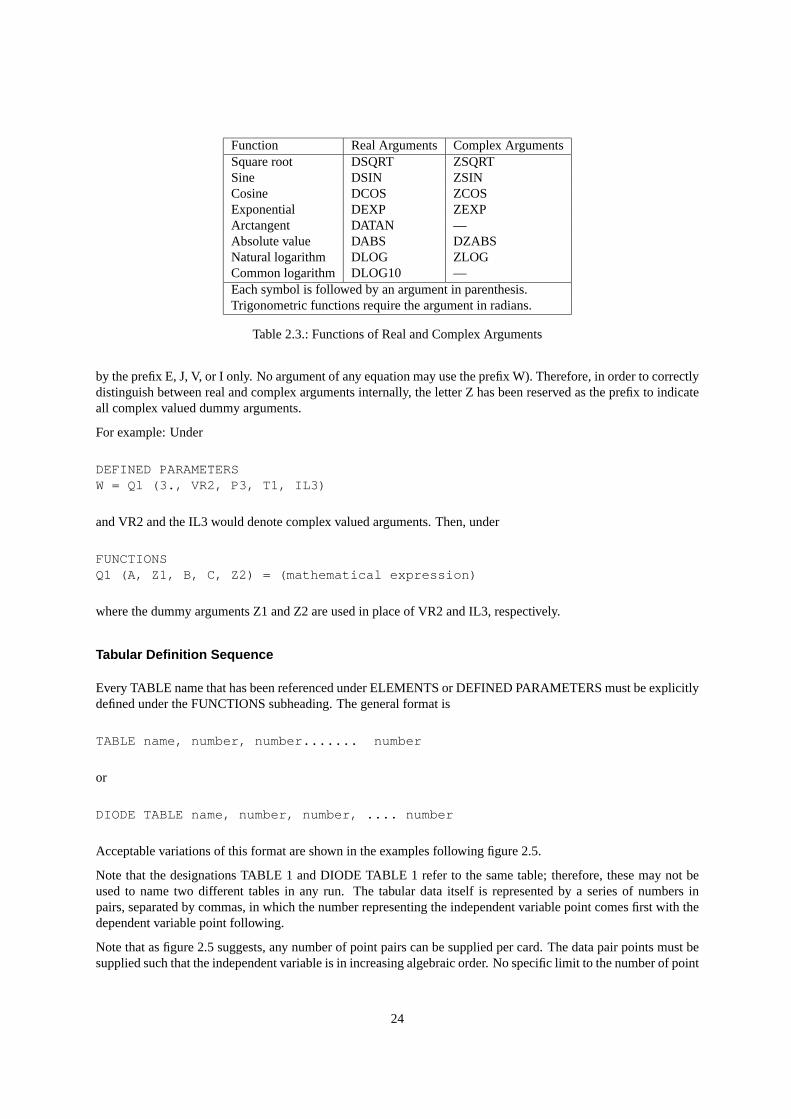
Function Real Arguments Complex ArgumentsSquare root DSQRT ZSQRTSine DSIN ZSINCosine DCOS ZCOSExponential DEXP ZEXPArctangent DATAN —Absolute value DABS DZABSNatural logarithm DLOG ZLOGCommon logarithm DLOG10 —Each symbol is followed by an argument in parenthesis.Trigonometric functions require the argument in radians.
Table 2.3.: Functions of Real and Complex Arguments
by the prefix E, J, V, or I only. No argument of any equation may use the prefix W). Therefore, in order to correctlydistinguish between real and complex arguments internally, the letter Z has been reserved as the prefix to indicateall complex valued dummy arguments.
For example: Under
DEFINED PARAMETERSW = Ql (3., VR2, P3, T1, IL3)
and VR2 and the IL3 would denote complex valued arguments. Then, under
FUNCTIONSQ1 (A, Z1, B, C, Z2) = (mathematical expression)
where the dummy arguments Z1 and Z2 are used in place of VR2 and IL3, respectively.
Tabular Definition Sequence
Every TABLE name that has been referenced under ELEMENTS or DEFINED PARAMETERS must be explicitlydefined under the FUNCTIONS subheading. The general format is
TABLE name, number, number....... number
or
DIODE TABLE name, number, number, .... number
Acceptable variations of this format are shown in the examples following figure 2.5.
Note that the designations TABLE 1 and DIODE TABLE 1 refer to the same table; therefore, these may not beused to name two different tables in any run. The tabular data itself is represented by a series of numbers inpairs, separated by commas, in which the number representing the independent variable point comes first with thedependent variable point following.
Note that as figure 2.5 suggests, any number of point pairs can be supplied per card. The data pair points must besupplied such that the independent variable is in increasing algebraic order. No specific limit to the number of point
24
7.fig
1
2
1 2 3 4TIME
TABLE ERIN
value
Figure 2.5.: TABLE ERIN Values as a Function of Time
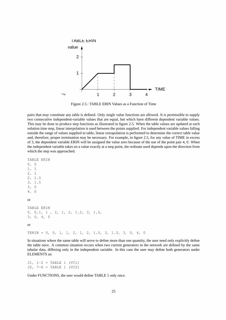
pairs that may constitute any table is defined. Only single value functions are allowed. It is permissible to supplytwo consecutive independent-variable values that are equal, but which have different dependent variable values.This may be done to produce step functions as illustrated in figure 2.5. When the table values are updated at eachsolution time step, linear interpolation is used between the points supplied. For independent variable values fallingoutside the range of values supplied in table, linear extrapolation is performed to determine the correct table valueand, therefore, proper termination may be necessary. For example, in figure 2.5, for any value of TIME in excessof 3, the dependent variable ERIN will be assigned the value zero because of the use of the point pair 4, 0. Whenthe independent variable takes on a value exactly at a step point, the ordinate used depends upon the direction fromwhich the step was approached.
TABLE ERIN0, 01, 12, 12, 1.53, 1.53, 04, 0
or
TABLE ERIN0, 0,1, 1 , 2, 1, 2, 1.5, 3, 1.5,3, 0, 4, 0
or
TERIN = 0, 0, 1, 1, 2, 1, 2, 1.5, 3, 1.5, 3, 0, 4, 0
In situations where the same table will serve to define more than one quantity, the user need only explicitly definethe table once. A common situation occurs when two current generators in the network are defined by the sametabular data, differing only in the independent variable. In this case the user may define both generators underELEMENTS as:
J1, 1-2 = TABLE 1 (VC1)J2, 7-8 = TABLE 1 (VC2)
Under FUNCTIONS, the user would define TABLE 1 only once.
25

2.2.7. Run controls
This subsection contains all the auxiliary information needed to control the run. The information does not directlyaffect the network. Most of these quantities have automatic default entries that hold unless specific entries aresupplied by the user. The default entries are given in table 2.4. All possible entries under the RUN CONTROLSsubheading are given in the following subsections. These entries may be made in any order, and as many may beplaced on a card as will fit, if they are separated by commas.
Run Limits
All transient runs must have a problem duration in the time units consistent with those used to describe the circuit.The form is simply:
STOP TIME = number
Since the user will never know in advance the computer time required for the solution of a given run, it maysometimes be desirable to enter a limit that will automatically terminate the run if that limit is exceeded. The limitin minutes may be entered as
COMPUTER TIME LIMIT = number
The preset value for COMPUTER TIME LIMIT is set to 600 minutes. This statement is active on IBM System/360computers where a system clock is installed and applies to total elapsed time. It should be noted that for operationunder OS/MVT the time used for the above statements is elapsed time as accumulated on the system clock and notCPU utilization time.
Another type of limit is available that operates on the number of passes made by the integration routine. In theabsence of any instruction from the user, the program imposes a limit of 20,000 passes. The user may change thislimit by entering.
INTEGRATION PASSES = number
Start Time
Most transient problems start at time equal to zero, and this entry may be omitted. Otherwise, the appropriate entryis:
START TIME = number
Integration Routine
Four integration routines are available for use with S/360 SCEPTRE. Three are explicit (XPO, TRAP and RUK)and one is implicit. (Implicit is not available on 7090/94.) The default option is XPO and, therefore, this methodis used unless one of the others is specifically requested. When one of the others is desired, the format is
INTEGRATION ROUTINE = TRAP
26

Quantity Default InformationSTOP TIME NoneCOMPUTER TIME LIMIT None (7090/94), 600 min (S/360)MAXIMUM INTEGRATION PASSES 20,000START TIME 0INTEGRATION ROUTINE XPOMINIMUM STEP SIZE 1 · 10−5 (STOP TIME) xpo, trap, ruk
1 · 10−14 (STOP TIME) implicitMAXIMUM STEP SIZE 2 · 10−2 (STOP TIME)STARTING STEP SIZE 1 · 10−8 (STOP TIME) xpo, trap,ruk
1 · 10−8 (STOP TIME) implicitXPO TRAP RUK IMPLICIT
MINIMUM ABSOLUTE ERROR .0001 .00005 .00005 .0001MAXIMUM ABSOLUTE ERROR .005 .001 .005MINIMUM RELATIVE ERROR .0002 .0005 .00005MAXIMUM RELATIVE ERROR .005 .01 .005Mode of Analysis Transient OnlyNEWTON-RAPHSON PASS LIMIT 100RELATIVE CONVERGENCE 0.001ABSOLUTE CONVERGENCE 0.0001MAXIMUM PRINT POINTS 1000COMPUTER SAVE INTERVAL 15VECTOR EQUATIONS 100 (transient) 70 (DC)XPLOT DIMENSION 10YPLOT DIMENSION 5TYPE FREQUENCY RUN LINEARNUMBER FREQUENCY STEPS 10COMPRESSION COUNT .3*(Input Function Buffer)RUN MONTE CARLO† 10INITIAL RANDOM NUMBER 127263527DISTRIBUTION GAUSSIANRUN OPTIMIZATION † 30MINIMUM FUNCTION ESTIMATE 0OPTIMIZATION CRITERION 10−7
OPTIMIZATION RANDOM STEPS 0RANDOM STEP SIZE CONTROL .2INITIAL H MATRIX FACTOR 1.RUN WORST CASE† NOMINAL†: Default value obtains when Run Control is entered without ’=number’.
If the Run Control itself is omitted, the indicated calculation will not occur.
Table 2.4.: Default run control quantities in SCEPTRE
27
or
INTEGRATION ROUTINE = RUK
or
INTEGRATION ROUTINE = IMPLICIT
Certain additional operations are required when implicit integration is used. These are performed internally ac-cording to a prescribed default mechanism, but the user may exercise control over the default. (See [2, subsection5.5].) Two possible statements are available.
USE DIFFERENCED JACOBIANUSE SYMBOLIC JACOBIAN
Use of the Convolution routine requires that the RUK integration routine be specified.
Minimum Step Size
Any transient run will automatically terminate whenever a time step size is required that is smaller than the min-imum step size. If this quantity is not supplied, the program will automatically compute a minimum limit. Forexplicit integration, this minimum limit is equal to 1 x 10⁻⁵ times the problem duration (STOP TIME). For im-plicit integration, the multiplying factor is 1 x 10⁻¹⁴. If a specific minimum step size independent of the problemduration is desired, the format is:
MINIMUM STEP SIZE = number
For example if, in a run using explicit integration,
STOP TIME- = 5000
is specified, the minimum size would automatically be 0.05. To change this to 0.01, use
MINIMUM STEP SIZE = 0.01
Maximum Step Size
This quantity sets an upper limit to the time solution increment that can be used to prevent a complete transientsolution composed of few solution points. If this quantity is not supplied, the program will automatically computea maximum limit equal to 2 x 10⁻² times the problem duration (STOP TIME). If a specific maximum step sizeindependent of the problem duration is desired, the format is:
MAXIMUM STEP SIZE = number
28

Starting Step Size
This quantity will be the size of the first time solution increment that is taken. Subsequent increments are automat-ically chosen by the integration routine. If this quantity is not supplied, the program will automatically compute astarting step equal to 1 x 10⁻³ for explicit, 1 x 10⁻⁸ for implicit, times the problem duration (STOP TIME). If aspecific starting step size independent of the problem duration is desired, the format is:
STARTING STEP SIZE = number
Error Criteria
Unless otherwise specified, any of the three explicit integration routines will operate with preset relative errorcriteria. If it is desired to modify these criteria, the proper formats would be:
MINIMUM ABSOLUTE ERROR = numberMAXIMUM ABSOLUTE ERROR = numberMINIMUM RELATIVE ERROR = numberMAXIMUM RELATIVE ERROR = number
The only error criterion that pertains to implicit integration is MINIMUM ABSOLUTE ERROR. The SCEPTREintegration routines are described in detail in [2].
Mode of Analysis
SCEPTRE can compute DC, AC, or transient solutions only, or certain combinations of these. The combinationsare DC with AC and DC with transient. Runs combining AC with transient cannot be made. The default modeof analysis is the transient run; that is, unless otherwise specified by the user, only the transient solution will becomputed. The transient solution can be run with or without convolution (see Appendix A.8).
SCEPTRE offers five DC solution modes: Initial Conditions, Sensitivity, Monte Carlo, Worst-Case and Opti-mization. Any of the five may be used alone, or as a source of initial conditions data for a Transient or AC run.Alternatively, the user may supply initial conditions data himself as entries to a Transient or AC run without thehelp of the DC options. One of the DC options, called Initial Conditions, takes part in all DC solutions. It may becalled separately, and if any other DC option is called, that option uses two or more passes of the Initial Conditionscalculation to produce its results. The Initial Conditions solution (and thus the other DC options) may use eitherthe Newton-Raphson or implicit method. Table 2.5 shows the entries, under RUN CONTROLS, used for eachmode of analysis.
If it is desired to run only DC solutions, the proper entry is:
RUN INITIAL CONDITIONS ONLY
plus the selected DC option, for which the entries are:
RUN SENSITIVITY
and/or
RUN MONTE CARLO
29

Mode of AnalysisDesired
RUN CONTROL Required RUN CONTROL Optional Notes
DC Solutions RUN INITIAL CONDITIONS ONLY RUN IC VIA IMPLICIT 1only RUN SENSITIVITY 2
RUN MONTE CARLO 2RUN WORST CASE 2RUN OPTIMIZATION 2
DC Plus Tran-sient
RUN INITIAL CONDITIONS or one or moreof the following
RUN IC VIA IMPLICIT 1
RUN SENSITIVITY 2RUN MONTE CARLO 2RUN WORST CASE 2RUN OPTIMIZATION 2plus STOP TIME = number
DC Plus AC same as above plus RUN AC RUN IC VIA IMPLICIT 1Transient only STOP TIME = number 3AC Only RUN ACTransient PlusAC
This combination is not possible
Table 2.5.: Run controls for specifying mode of analysis
and/or
RUN WORST CASE
and/or
RUN OPTIMIZATION
(See subsection 2.2.7 for more detailed discussion of the Sensitivity, Monte Carlo, Worst-Case and OptimizationRun Controls.)
Any one or more of the above five entries will cause Initial Conditions to be found by the Newton- Raphsonmethod. If it is desired that the DC solutions be run using the Implicit technique, include the extra entry
RUN IC VIA IMPLICIT
(See Appendix A.3 for a discussion of the Implicit Method of computing Initial Conditions.)
Notes:
1. The entry RUN IC VIA IMPLICIT will cause all requested DC solutions to use the implicit methods. If thiscard is not entered, all requested DC solutions will be by the Newton-Raphson method.
2. DC solutions are accomplished in the order shown in this table. See text.
3. Transient only is the default mode of analysis.
30

The user should note that the method he chooses, either Newton-Raphson or Implicit, for finding Initial Conditionswill be used in all DC solutions he requests on the same run. Thus, the choice of the method for a particularproblem can have a sizeable effect on running time when several DC calculations are involved. The user shouldthus exercise care in the selection of the Initial Conditions method.
The user should also note that the DC runs are performed in the order Sensitivity, Monte Carlo, Worst-Case andOptimization, regardless of the order in which the cards are entered. Thus, if the user desires to use the results ofany particular DC computation as initial conditions for the transient or AC solution to follow, he must not requestany of the DC options which appear after it in the above mentioned order. For instance, if the user wishes to usethe results of a Monte Carlo solution as initial conditions for a transient (or AC) solution, he must not enter a RUNWORST CASE or RUN OPTIMIZATION card, or these DC solutions will remove the Monte Carlo data from thevoltages, currents, and defined parameter tables.
If the entry
RUN INITIAL CONDITIONS ONLY
is omitted, a transient solution will follow the DC solutions. If the user desires an AC analysis, with or without aDC analysis, the entry is:
RUN AC
plus entries for any DC analysis desired.
Under normal computational circumstances, the initial conditions for any rerun are either inserted by the user orcomputed by the DC portion of the program (see subsections 2.4.1 and 2.4.2). There may be situations, however,in which it is desirable to have the results of master runs, either AC, DC or transient, used as the starting values forone or more associated reruns.
If it is intended that all associated reruns use the final values of the master run as initial conditions, the appropriateentry under RUN CONTROLS is:
IC FOR RERUNS = MASTER RESULTS
If it is intended that each rerun use the final result of the preceding rerun in the sequence, the entry is:
IC FOR RERUNS = PRECEDING RESULTS
(See Appendix A.3 for additional information.)
Convergence of the Newton-Raphson Routine
The Newton-Raphson iteration method should produce convergence and, hence, d-c solutions in less than 30 passesfor most networks. If convergence is slow or does not occur, some realistic limit should be placed on the numberof passes that are made. Unless otherwise specified, a limit of 100 passes is built into SCEPTRE. To change thislimit, the proper entry is:
NEWTON-RAPHSON PASS LIMIT = number
31

Convergence is considered to have occurred if
|Y (n)− Y (n− 1)| ≤ A ∗ |Y (n)|+B,
where Y refers to the vector of initial condition state variables, n is the number of completed passes, A is therelative criterion, and B is the absolute criterion. The values A = 0.001, B = 0.0001 are built into SCEPTRE. Theuser probably will not want to change these values, but if either quantity is to be changed, the proper entries are:
RELATIVE CONVERGENCE = numberABSOLUTE CONVERGENCE = number
Output Control
Some transient runs may require thousands of solution points, and it is usually unnecessary to have every solutionprinted out. SCEPTRE is processed to output a maximum of 1000 spaced points regardless of the number of stepstaken. The maximum number of printed output points may be changed for any particular run by entering:
MAXIMUM PRINT POINTS = number
An additional means exists by which the number of solution points may be precisely controlled and chosen moreselectively. The user supplies the desired time interval and only those solution points that fall on or immediatelyafter integer multiples of the specified interval will be printed in this series. The required entry is;
PRINT INTERVAL = number
This printed series will appear in addition to the normal printed output format. If only this printed series is desired,the normal printed output format may be suppressed by the entry:
MAXIMUM PRINT POINTS = 0
(For additional discussion of print interval, see Appendix A.4.)
A discussion of the PLOT INTERVAL run control, used to control the length of composite plots may be found insubsection 2.2.4.
Automatic Termination of Transient Runs
The user may often desire to monitor certain voltages or currents in a network to determine their relation with somepredetermined quantity. If the relations are satisfied, there may be no further interest in continuing the run. Therun can be terminated at that point by the entry:
TERMINATE IF (XXXXXX relational operation XXXXXX)
The X quantities refer to any variable or constant. The user frequently supplies some element voltage or currentfor this purpose. The following relational operators may be used:
.LE. less than or equal to
32

.LT. less than
.GT. greater than
.GE. greater than or equal to
.EQ. equal to
.NE. not equal to
NOTE: Decimal points are required before and after an operator. A typical entry would be:
TERMINATE IF (VCC .GT. 0.)
which would automatically terminate that particular run whenever the voltage across capacitor CC became positive.
The termination feature may be extended to cover AND/OR logical situations by using the logical operators .AND.and .OR.. A legal entry could be:
TERMINATE IF ((VCC .GT. 0.) .OR. (IL17 .GE. 7.))
This would terminate the run if the voltage across capacitor CC became positive or the current through inductorL17 exceeded 7 units of current. The other logical possibility would be simply
TERMINATE IF ((VCC .GT. 0.) .AND. (IL17 .GE. 7.))
All automatic Termination conditions must apply to all reruns that are associated with a given master run (seeSection 2.4.1). One variation is available. If it is desired that all remaining reruns be canceled if a terminationcondition is met, the word STOP is used instead of TERMINATE. Then a typical entry would be:
STOP IF (VCC .GT. 0.)
Computer Save Interval
Particularly long computer runs should be protected against complete loss arising from improper terminationcaused by electrical malfunction, operator error, etc. This is done by periodically recording the status of therun on tape such that it can always be continued from the last saved point if improper termination does occur. A15-minute save interval is preset in the program which ensures that no more than 15 minutes of computer solutiontime can ever be lost in this way. The user may change the save interval to any number of minutes of computersolution time by the entry:
COMPUTER SAVE INTERNAL = number
33

Run Controls for DC Options
This paragraph describes the Run Controls for the four special DC options, Sensitivity, Monte Carlo, Worst-Caseand Optimization. See subsection 2.2.7 for a discussion of the use of these options in combination with each other,with the normal Initial Conditions calculations, and with the Transient and AC calculations.
In addition to the Run Controls discussed below, use of the DC options requires entries under the correspondingCIRCUIT DESCRIPTION subheadings (SENSITIVITY, MONTE CARLO, WORST-CASE or OPTIMIZATION)listing the dependent and independent variables to be used in the calculations. (See subsection 2.2.8.) Use ofMonte Carlo, Worst-Case and Optimization also requires bounds on entries under ELEMENTS and DEFINEDPARAMETERS. (See subsections 2.2.2 and 2.2.3.)
Sensitivity calculation requests are made by the entry:
RUN SENSITIVITY
There are no additional Run Controls for Sensitivity.
The Monte Carlo calculation is initiated by use of either:
MONTE CARLO = number
or
RUN MONTE CARLO
The number specified is the count of Monte Carlo iterations to be performed. If the count is unspecified, it isassumed to be 10.
The distribution to be used for random variables in a Monte Carlo run is selected by use of one of the controls;
DISTRIBUTION = GAUSSIAN
or
DISTRIBUTION = UNIFORM
If neither is specified, the Gaussian distribution is used. The initial random number is specified by use of thecontrol:
INITIAL RANDOM NUMBER = number
The number used should be a nine-digit positive odd integer. If no initial number is specified, a suitable number isprovided by SCEPTRE. If it is important to have all reruns start with the same random number, the statement:
INITIAL RANDOM NUMBER = DEFAULT
may be used. If this entry is not used, SCEPTRE will select a different initial random number for each rerun.
Optional printed information from each Monte Carlo iteration is obtained by inclusion of the statement:
34

LIST MONTE CARLO DETAILS
The Worst-Case calculations will be executed if one of the Run Controls:
WORST CASE = LOWWORST CASE = NOMINALRUN WORST CASE = HIGH
is provided. The word following the equal sign determines the set of values to be left in the elements, voltages,currents and defined parameter tables at the conclusion of the Worst-Case calculation, for use as initial conditionsin a subsequent transient calculation. LOW and HIGH refer, respectively, to those table values which producethe smallest and largest value of the last objective function requested in the list entered under the WORST CASEsubheading of CIRCUIT DESCRIPTION (see subsection 2.2.8).
If the control:
RUN WORST CASE
is used, the nominal values are restored to the tables at the conclusion of the Worst-Case calculation.
The Optimization process will be run if the Run Control
OPTIMIZATION = integer
appears, and if the appropriate entries are made under the OPTIMIZATION subheading (see subsection 2.2.8). Theinteger which appears after the equal sign indicates the maximum number of optimization iterations which will beallowed for any objective function. If the number is omitted, thirty iterations will be allowed.
Since Optimization can be a time-consuming process and may, in fact, fail if the network has pathological behavior,additional Run Controls have been provided to assist the user. If the card
LIST OPTIMIZATI0N DETAILS
is used, auxiliary intermediate results will be provided to the user. If he supplies the Run Control
PUNCH OPTIMIZATION RESULTS
the most recently updated values of the approximate inverse Hessian matrix (see [2, subsection 2.4.5]), of thegradient vector and of other parameters will be punched out. Thus, if the user wishes to limit the number ofOptimization iterations until he examines the progress of the process, he can save the intermediate results for usein reinitializing at a later run. To be utilized, these punched values, must be provided as data cards in the SCEPTREdeck (see Section??), and the card format
INITIAL H MATRIX FACTOR = 0
must be included among the Run Controls.
If this Run Control is used with a non-zero number, no attempt will be made to read previously punched values.Instead, the number will be used to scale the initial approximation to the inverse Hessian. Careful use of anypre-knowledge about the scale of the inverse matrix can improve optimization performance. If this Run Control isnot entered, the initial approximation is the unit matrix.
The tolerance within which the value of objective function should be located is provided by the Run Control
35

OPTIMIZATION CRITERION = number
If this card does not appear, the iteration will stop whenever the estimated improvement will be less than 10−7.Note that in the presence of a broad, shallow minimum, the objective function will be relatively insensitive to thevalues of the independent variables. In this case, even a small objective function tolerance will permit the programa wide latitude in its choice of final values of the independent variables.
Under some conditions, particularly with a shallow minimum as described above, the algorithm may not locate atrue minimum because the error criterion permits it to stop at a ’neighboring’ point in the space of the independentvariables. To protect against this possibility, two additional Run Controls have been implemented. If the RunControl
OPTIMIZATION RANDOM STEPS = integer
appears, displacements in random directions from the assumed minimum will be made the indicated number oftimes, and the function re-minimized each time. The smallest value resulting from the random motion and re-optimization should be accepted as the true minimum. If the Run Control
RANDOM STEP SIZE CONTROL = number
is used, the independent variable steps an amount estimated to increase the value of the function by 0.5*(num-ber)**2 above its minimum at each random displacement. If this Run Control is not used, the value 0.2 is used.
The formulation of the Davidon method requires that the objective function minimum value be positive. Since thisis not always the case, provision has been made within SCEPTRE to effectively maintain the objective functionpositive by addition of a suitable positive number. However, if the user has some estimate of the true minimumvalue, he may enter his own reference value and thereby improve the performance of the optimization. The correctform of this Run Control is:
MINIMUM FUNCTION ESTIMATE = number
Note, however, that the value entered will apply to all objective functions specified under the OPTIMIZATIONsubheading.
Convolution Run Controls
The insertion of one or more Convolution Model Calls under ELEMENTS (see table 2.2) causes SCEPTRE torequest the Convolution Option as part of a transient run. Four Run Controls are used to regulate the Convolutionoption2 These Run Controls are in addition to those described above for the transient run proper. Of the fourConvolution Run Controls, two regulate the run and define the storage required, and two are associated with theoptional CMPAC routine, which provides in-process smoothing of the calculated results, with attendant saving ofstorage space.
The first two Run Controls allocate internal core storage for the two functions associated with the Convolutionprocess. These Run Controls are:
IMPULSE RESPONSE BUFFER = number
and2Use of Convolution requires that the RUK integration routine be specified. RUK is not the default integration mode. (See subsection 2.2.7.)
36

INPUT FUNCTION BUFFER = number
where number, in the first instance, is the average number of storage points required per impulse response functionand, in the second, is the number of points required to store each corresponding kernel’s input function. (Theinput functions are SCEPTRE-generated, and an equal number of storage spaces must be set aside for each.) If theallocated storage space is exceeded, the run will terminate.
The other two Convolution Run Controls are optional. They call and control the internal compression routine.Without CMPAC, the user must anticipate the number of steps the program might take, and then allocate enoughstorage space via the INPUT FUNCTION BUFFER mechanism. This approach obviously makes increasing de-mands on storage as either the number of convolution kernels or the number of desired integration steps increases.The CMPAC routine reduces the total core storage required by Convolution, by compressing the SCEPTRE-generated data tables that are convolved internally with the impulse response functions. The first of the RunControls which invoke and regulate this compression routine is:
COMPRESSION COUNT = integer
where integer, which must be no greater than that set in by INPUT FUNCTION BUFFER, is used to indicate thenumber of successful integration steps taken between successive calls to CMPAC. The second entry is used in theinternal decision-making process to determine if intermediate points need to be retained. This CMPAC control is:
COMPRESSION CRITERION = constant
where constant *100 indicates the maximum percentage area which may be lost due to omitting the middle pointof any three consecutive data points. For one pass through the algorithm, this is also the maximum total percentagearea lost due to leaving out all possible middle points. However, the routine is repeatedly cycled through untilno more points can be removed. For each additional pass this COMPRESSION CRITERION is automaticallytightened by a factor of four.
Because of this tightening and repetition process, the maximum possible percentage loss, over a series of com-pressions can exceed the value set in by the COMPRESSION CRITERION entry. For normal criteria (up to .05),however, the maximum total loss on all passes could not exceed the criterion by more that 25 percent (or from .05to .0625, for example).
Run Controls for AC Analysis
AC Analysis is called by use of the Run Control
RUN AC
Frequencies at which the analysis is to be carried out are specified in one of two ways. If the response at a singlefrequency is desired, the single entry under RUN CONTROLS
FREQUENCY = number
is used. Number, in the above entry, is the desired single frequency. If, however, the response is desired over arange of frequencies, the following sequence of three entries is used:
INITIAL FREQUENCY = numberFINAL FREQUENCY = number
37

where number in each case denotes a frequency, and
NUMBER FREQUENCY STEPS = number
where number is the number of intervals desired (one less than the number of calculations to be made). This entrymay be omitted. The default value is ten (eleven calculations).
If linear frequency spacing is desired, the control
TYPE FREQUENCY RUN = LINEAR
may be used. If logarithmic spacing is to be used, the proper control is:
TYPE FREQUENCY RUN = LOG
if neither of these two entries is supplied, the default value is linear.
If circuit ELEMENTS (other than source values) are not varied in reruns, computation time for the eigensolutionportion of the analysis can be saved by inclusion of the Run Control:
USE FIXED AC MATRIX IN RERUNS
Additional Run Controls
There are seventeen additional Run Controls in SCEPTRE which are not described in subsection 2.2.7. These RunControls either have semi-diagnostic roles or are best explained within the detailed discussion of functions theycontrol. Table 2.6 lists these Run Controls and the paragraphs which describe them.
2.2.8. DC options
Subheadings under the CIRCUIT DESCRIPTION heading are provided for the user to identify the variables hewishes treated in the Sensitivity, Monte Carlo, Worst-Case and Optimization calculations. The input data consistsof the appropriate subheading:
SENSITIVITYMONTE CARLOWORST CASE
or
OPTIMIZATION
followed by the appropriate parameters. Each set of parameters is enclosed in parentheses. The objective func-tions or dependent variables are listed first, followed by a slash and the list of independent variables. Individualvariables in the list are separated by commas. Each set must name at least one dependent variable and at least oneindependent variable3. The form is:
(dependent variable list / independent variable list)
38

Run Control See Subsection RemarksPRINT A MATRIX 2.8.5 AC DiagnosticPRINT EIGENVALUES 2.8.5 AC DiagnosticPRINT EIGENVECTORS 2.8.5 AC DiagnosticLIST NODE MAP 2.8.4 Network DiagnosticX PLOT DIMENSION —Y PLOT DIMENSION —SOLUTION TIME LIMIT —NO ELEMENT SORT 2.8.2PRINT B MATRIX 2.8.3PUNCH PROGRAM —FULIST —PUNCH BINARY CARDS —WRITE SIMUL8 DATA 2.8VECTOR EQUATIONS —WRITE DEBUG 2.8.6 Prints Internal Program DataEXECUTE SETUP PHASE ONLY —PLOT INTERVAL 2.2.4 Used with composite Plots. Omission
results in deletion of Composite Plots.
Table 2.6.: Additional run controls
Allowable dependent variables are listed in table 2.7. Allowable independent variables are listed in table 2.8.The Sensitivity, Worst-Case and Optimization solutions use Adjoint Calculations as discussed in [2]. Adjointcalculations give the partial derivatives of dependent variables with respect to a list of independent variables.There is no specific limit on the total number of dependent variables or independent variables. The limit is onsets of variables. A set is a list of dependent variables, together with its list of independent variables. The totalnumber of all sets entered for Sensitivity plus Worst-Case plus Optimization must not exceed one hundred. Also,four times the total number of dependent variables plus the total number of independent variables must not exceedfour hundred. The total number of Monte Carlo sets must not exceed forty. Four times the number of Monte Carlodependent variables plus the total number of Monte Carlo independent variables must not exceed one hundred.
An example of valid Sensitivity input data cards is:
SENSITIVITY(IL3, PX/JX,EY)(VR1, IR1, VCX/P1,E1)
In this example the following partial derivatives would be calculated:
∂IL3∂JX
∂IL3∂EY
∂PX
∂JX
∂PX
∂EY
∂V R1∂P1
∂V R1∂E1
∂IR1∂P1
∂IR1∂E1
∂V CX
∂P1∂V CX
∂E1
An example of Optimization input data is:
OPTIMIZATION(IR1, P1/R1,P2,E1)(VC1/J1,R2)
In this example3For Monte Carlo, Worst-Case and Optimization calculations, the independent variables named here must be specified, with bounds, underthe ELEMENTS sub-headings of CIRCUIT DESCRIPTION (see subsection 2.2.2)
39

Name Description (see Table 2.2)VC Voltage across a capacitorIE Current through an independent voltage sourceJ Value of a primary dependent current sourceVJ Voltage across an independent current sourceIL Current through an inductorIR Current through a resistorVR Voltage across a resistorP Defined Parameter†
†: For a Sensitivity, Optimization, or Worst Case dependent variablePname, the differential GPname must also be supplied (see subsection2.2.3)
Table 2.7.: Dependent variables in DC calculations.
Name Description (see Table 2.2)R ResistorE Independent Voltage SourceJ Independent Current SourceP Defined Parameter‡
‡: A defined Parameter independent variable can only be the factor in asecondary dependent current source definition, e.g., J0=Pname*J9. Seesubsection 2.2.3 for the format of defined parameters with bounds.
Table 2.8.: Independent variables in DC calculations.
• IR1 is optimized with respect to R1, P2, E1
• P1 is optimized with respect to R1, P2, E1
• VC1 is optimized with respect to J1, R2.
An example input for Worst-Case calculation would take a form like those above under a
WORST CASE
subheading.
2.2.9. Program limits
7090/94 only:
The standard core memory capacity available on the IBM 7090/94 data processing system is 32,000 words, whichimposes certain program limits on the capacity of the SCEPTRE program. Two factors that establish these limita-tions are program storage and data storage.
The program storage requirements have priority over data storage and must be satisfied first. The entire SCEPTREprogram would require approximately 64,000 words of core storage, but this capacity is not necessary if the overlayfeature of the IBSYS monitor system is used. This feature breaks up the program into several segments called’links’ which are executed sequentially. Each segment overlays or occupies the portion of core storage used by thepreceding segment. Therefore, the amount of program storage required is equal to the largest program segment.
40

The storage capacity that remains after the program storage requirements are satisfied is available for data. Inthe SCEPTRE program, there are about l0,000 words of storage available for this purpose. Within this area,the program data are limited by FORTRAN dimension statements which allocate specific amounts of storage.Although these limits are usually considered fixed, they can be changed somewhat by a programmer. However,increasing limits in this manner usually is accomplished by decreasing one or more of the other program datalimits. Also, any change which affects the total amount of data storage will necessitate a change to the programstorage, and therefore, the program.
S/360 only:
The main storage capacity on the IBM System/360 Data Processing System is facility dependent. It is recom-mended that the user consult with a system programmer concerning the main storage available for problem pro-grams. The disseminated version of the System/360 SCEPTRE is set up for OS/MVT operation and requires a224k byte region. The program data limits remain unchanged.
Table 2.9 gives the program data limits which have been established in the program as it is distributed. These limitsare considered adequate for most normal circuit analysis work. Approximate limits are also given for the numberof TABLE and EQUATION functions.
If only one-half of an input card is used to write the equation specification, 160 equation functions could be used.Conversely, if each equation specification took two full data cards, only 40 equations would be allowed. Definingtable functions involves a similar process, which considers the number of x-y coordinates and the number of tables.Forty tables, each containing 20 point pairs, or eight tables each containing 100 point pairs would be allowed.
The limits shown in table 2.9 are checked by SCEPTRE as the data is read into storage. If any limits are exceededa message stating the limit is produced, and the computer run terminated.
The alphanumeric character limits are listed in table 2.10. The circuit designation used for models is alwaysappended to any names used in a model description and the combined total characters must not exceed the circuitdescription limits. For example, element CB in a model designated as T15 in the circuit description becomesCBT15.
2.2.10. Vectorized notation
When large networks are encountered, SCEPTRE automatically reverts to an internal renaming feature (VECTOR-IZED NOTATION) which effectively enlarges the capacity of the FORTRAN Compiler. ’Large’ networks, in thiscase, refer to those containing 70 or more elements if a DC solution is requested, or 100 or more elements if onlya transient solution is to be made. This feature will not affect the user operationally as long as the input formatsgiven in this manual are followed. It will, however, cause SIMUL8 to be written in terms of the renamed quantities.A complete listing of all circuit Elements and Defined Parameters along with their corresponding internal nameswill be provided for every run in which renaming occurs.
2.2.11. Internal Parameters
A number of parameters are carried internally in the program. The user has permitted access to these parametersfor use as Equation arguments, independent variables for tables, and automatic termination quantities and outputs.The nomenclature and definitions of these parameters are given in Table 2.11.
41
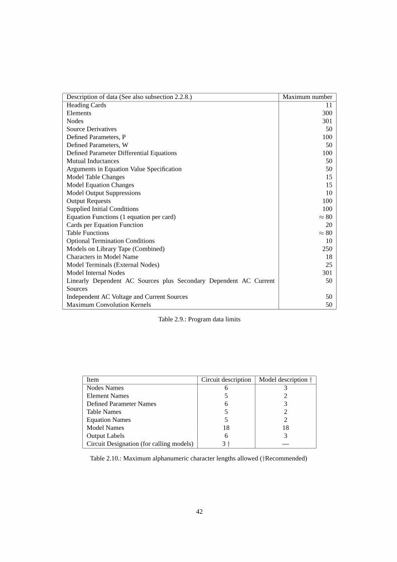
Description of data (See also subsection 2.2.8.) Maximum numberHeading Cards 11Elements 300Nodes 301Source Derivatives 50Defined Parameters, P 100Defined Parameters, W 50Defined Parameter Differential Equations 100Mutual Inductances 50Arguments in Equation Value Specification 50Model Table Changes 15Model Equation Changes 15Model Output Suppressions 10Output Requests 100Supplied Initial Conditions 100Equation Functions (1 equation per card) ≈ 80Cards per Equation Function 20Table Functions ≈ 80Optional Termination Conditions 10Models on Library Tape (Combined) 250Characters in Model Name 18Model Terminals (External Nodes) 25Model Internal Nodes 301Linearly Dependent AC Sources plus Secondary Dependent AC CurrentSources
50
Independent AC Voltage and Current Sources 50Maximum Convolution Kernels 50
Table 2.9.: Program data limits
Item Circuit description Model description†Nodes Names 6 3Element Names 5 2Defined Parameter Names 6 3Table Names 5 2Equation Names 5 2Model Names 18 18Output Labels 6 3Circuit Designation (for calling models) 3 † —
Table 2.10.: Maximum alphanumeric character lengths allowed (†Recommended)
42

Int. name DefinitionXSTOPT Transient solution duration (STOP TIME)XIR Integration routine (TRAP=1, RUK=2, XPO=3)XTISSS Starting step sizeXMNISS Minimum step size allowedXMXISS Maximum step size allowedXMNAIE Minimum absolute errorXMXAIE Maximum absolute errorXRERNO Rerun numberXMXPAS Maximum pass limitXMNRIE Minimum relative errorXMXRIE Maximum relative errorXMXICP Newton-Raphson pass limitXICRER Newton-Raphson relative convergenceXICAER Newton-Raphson absolute convergenceXMXOTP Maximum number of print pointsXICPAS Newton-Raphson pass numberXNOPRQ Number of output requestsXNDFEQ Number of differential equationsXERT Elapsed computer timeXSTPNO Transient solution step numberXPASNO Transient solution pass numberXRUNNO Run number (including reruns)XSTPSZ Transient solution step sizeXSAVE Save intervalXTMON Elapsed computer time at start of transient solutionFREQ FrequencyTIME TimeXPLTI Plot IntervalXPRTI Print IntervalXINFRQ Initial FrequencyXFNFRQ Final FrequencyXTYPFQ Type Frequency RunXNFRQS Number of Frequency StepsXNMCPS Number of Monte Carlo SamplesXNOPPS Maximum number of Optimization Passes per StepXWCLHN Type of Worst-Case Results to be left as Initial Values for Transient RunXDISTR Type of Monte Carlo DistributionXACRE Use Fixed AC Matrix in RerunsXNCONV Number of Convolution kernels enteredXHAVE Impulse Response Buffer Storage AllocationXIAVE Input Function Buffer Storage AllocationXCMPCR Compression CriterionXCMPCT Compression CountXOPCR Optimization CriterionXNOPRS Number of Optimization Random Steps Remaining to be ExecutedXRNSSC Random Step Size ControlXHHFAC Initial H Matrix FactorXMNFES Minimum Function EstimateXSAVIC Type of Rerun InitializationXMXERT Computer Time Limit
Table 2.11.: Internal parameter table
43

2.3. Stored model feature
All active devices must be represented in SCEPTRE by combinations of R, L, C, M, E, and J. Most users willfind that repeated use is made of certain models of active devices or of standard combinations of passive elements,such as filter sections, biasing networks, etc. These situations can always be handled by inserting the componentsone by one in a CIRCUIT DESCRIPTION under ELEMENTS. A more convenient approach is to describe themodel or network once and store it for future use. The stored model feature is not ’free’; its use requires extratape manipulation, and hence, more computer time. However, the time saved in circuit preparation and the addedflexibility will compensate for the extra time.
The stored model feature of SCEPTRE is especially flexible since the user stores whatever models meet his specificneeds. A model may be stored permanently or temporarily. If it is stored permanently, the model may be calledout for insertion in a main network as often as desired per run and for any number of runs. The user might desireto reserve this type of storage for proven models that will see reasonably frequent service. Temporary storage, onthe other hand, stores a model for one run only (plus whatever reruns may be made during that run). This type ofstorage will probably prove most useful for experimental models or for models that are seldom used.
All stored models are transferred from storage to the main circuit where they are used by reference to their ex-ternal nodes or terminals. The user must ensure that corresponding nodes in both the main circuit and the storedmodel match in sequence. Internal nodes of any stored model are of no particular significance and will be brieflymentioned later.
The stored model feature is best illustrated by an example. Assume that the stored transistor model in figure 2.6bis to be inserted into the main circuit in figure 2.6a. The stored model contains terminal nodes 1, 2, and 3 (whichcorrespond to the base, emitter, and collector nodes of the transistor) and internal nodes 7 and 12. The main circuitmay also contain nodes 1, 2, 3, 7, or 12 without danger of ambiguity. Assuming that the model was originallystored with the node sequence 1, 2, and 3, the user could enter the following under ELEMENTS of the mainprogram:
T1 14-21-23 = MODEL X476900 (PERM)
This will match nodes 14, 21, and 23 of the main circuit with nodes 1, 2, and 3 of the stored model. The circuitdesignation of the stored model is T1 and the name of this particular stored model is X476900. The stored modelis transferred from the tape into the main circuit and nodes 1, 2, and 3 of the model become nodes 14, 21, and 23of the main circuit. Internal nodes 7 and 12 become 7 T1 and 12 T1 in the main circuit, because all internal nodesof stored models have appended to them the circuit designation of that model. Since no node name may containmore than six alphanumeric characters the user should use as few characters as possible for the circuit designationnames and internal nodes of any stored model.
2.3.1. Transistor model insertion
Transistors deserve special mention because of the frequency with which they occur in contemporary networks.The remainder of this section given the rules by which the user may store models of his choice.
Permanent Storage
Any three-terminal transistor may be permanently stored on tape using the following format after the MODELDESCRIPTION card:
MODEL name (PERM) (B-E-C)
44
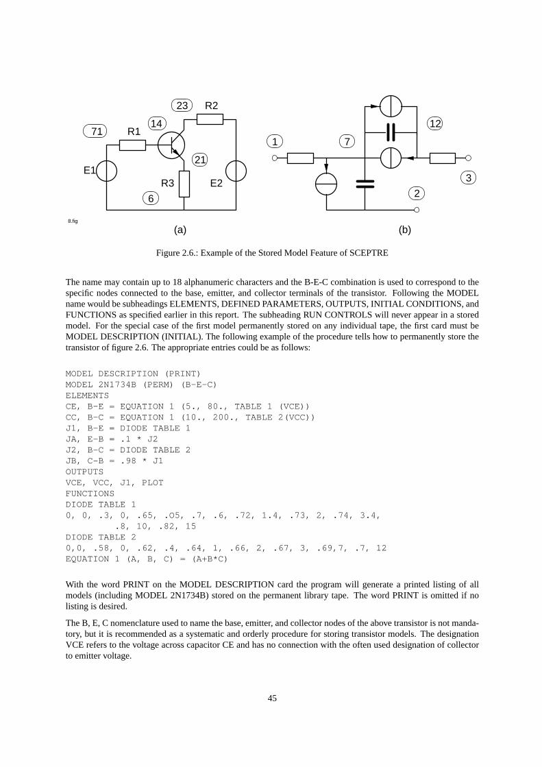
1271
21E1
R3 E2
6
R1
R223
14
71
2
3
(a) (b)8.fig
Figure 2.6.: Example of the Stored Model Feature of SCEPTRE
The name may contain up to 18 alphanumeric characters and the B-E-C combination is used to correspond to thespecific nodes connected to the base, emitter, and collector terminals of the transistor. Following the MODELname would be subheadings ELEMENTS, DEFINED PARAMETERS, OUTPUTS, INITIAL CONDITIONS, andFUNCTIONS as specified earlier in this report. The subheading RUN CONTROLS will never appear in a storedmodel. For the special case of the first model permanently stored on any individual tape, the first card must beMODEL DESCRIPTION (INITIAL). The following example of the procedure tells how to permanently store thetransistor of figure 2.6. The appropriate entries could be as follows:
MODEL DESCRIPTION (PRINT)MODEL 2N1734B (PERM) (B-E-C)ELEMENTSCE, B-E = EQUATION 1 (5., 80., TABLE 1 (VCE))CC, B-C = EQUATION 1 (10., 200., TABLE 2(VCC))J1, B-E = DIODE TABLE 1JA, E-B = .1 * J2J2, B-C = DIODE TABLE 2JB, C-B = .98 * J1OUTPUTSVCE, VCC, J1, PLOTFUNCTIONSDIODE TABLE 10, 0, .3, 0, .65, .O5, .7, .6, .72, 1.4, .73, 2, .74, 3.4,
.8, 10, .82, 15DIODE TABLE 20,0, .58, 0, .62, .4, .64, 1, .66, 2, .67, 3, .69,7, .7, 12EQUATION 1 (A, B, C) = (A+B*C)
With the word PRINT on the MODEL DESCRIPTION card the program will generate a printed listing of allmodels (including MODEL 2N1734B) stored on the permanent library tape. The word PRINT is omitted if nolisting is desired.
The B, E, C nomenclature used to name the base, emitter, and collector nodes of the above transistor is not manda-tory, but it is recommended as a systematic and orderly procedure for storing transistor models. The designationVCE refers to the voltage across capacitor CE and has no connection with the often used designation of collectorto emitter voltage.
45

After this model is stored permanently, it may be called upon as often as required. The user should use as fewalphanumeric characters as possible to represent individual elements in stored models because the program mustcombine the element name with the circuit designation given under ELEMENTS (but not with the model name). Ifthe above stored model is used in a network designated T11, the program must refer to the base-emitter capacitanceas CET11. In this case, the maximum number of five alphanumeric characters has been used for a given element.If either the circuit designation or the element name contained more characters, the run would be aborted. Thisconsideration is independent of the model name.
Temporary Storage
Each model intended for temporary storage must be described element by element under MODEL DESCRIPTIONin the run in which it is to be used. The words INITIAL and PRINT are never used on the MODEL DESCRIPTIONcard for temporary storage. The rest of the entry format is the same as for permanent storage except the wordTEMP:
MODEL name (TEMP) (node-node-node)
or
MODEL name (node-node-node)
If neither TEMP or PERM is used the program will automatically assume temporary storage.
After the model is stored, the circuit designation format in the main program for temporary models differs slightlyfrom the format used for permanent models. Where a permanently stored model is designated as:
T1, 7-8-9 = MODEL X476900 (PERM)
a temporarily stored model could be designated as
T1, 7-8-9 = MODEL X476900 (TEMP)
or
T1, 7-8-9 = MODEL X476900
2.3.2. N terminal model storage
The storage of N terminal models differs from the storage of transistor models only in the number of terminalnodes (program limit 25 nodes) that are specified. Storage may be effected by an entry following the MODELDESCRIPTION card as:
MODEL name (PERM or TEMP) (node-node-....node)
As many internal nodes as desired may be included within the program limit of 301 nodes. The remainder of theinformation will be entered under the appropriate subheadings. Regardless of the number of terminal nodes thatare supplied, the user must take care that these nodes are referenced in the same sequence when called by the mainprogram.
46
2.3.3. Changes to a stored model
The user who frequently makes use of the stored model feature of SCEPTRE will often encounter the situation inwhich the topology of his stored model is satisfactory but the size of some of the model elements must be changed.Changes can be effected easily for any individual run, but no permanent changes to the stored model are possible.(The user has the option of storing a second model which contains a different version of the original). All changesmust be indicated along with the statement that locates the stored model in the main circuit. This will always beunder the main circuit ELEMENTS subheading.
Changes in ELEMENTS or DEFINED PARAMETERS
Consider that a stored model has been called out as:
T1, 7-8-12 = MODEL 2N1734B
In this case, the model will be inserted into the main circuit as it was originally stored. If a change is desired inone or more internal elements or defined parameters of the stored model, the proper entry could be:
T1, 7-8-12 = MODEL 2N1734B (CHANGE CC = 50)
In this case, CC of the original model has been changed to 50 units of capacitance, regardless of its original formor size, All other elements in the stored model would remain as originally stored.
Another practical situation could be reflected by the entry:
T1, 7-8-12 = MODEL 2N1734B (CHANGE CC = TABLE 7 (VCCT1),JA = .2 * J2T1, JE = DIODE TABLE 4)
In this case, CC of the original stored model has been changed to a tabular function which must be represented(TABLE 7) under the FUNCTIONS subheading of the main circuit. Also, JA has been changed to a different math-ematical definition and JE has been changed to another tabular function which must appear under FUNCTIONS.The other elements of the stored model will remain in their original forms.
As a final example, assume that it is desired to change CC in a stored model to a different equation. Then:
T1, 7-8-12 = MODEL 2N1734B (CHANGE CC = EQUATION 5 (VCCT1, VCX))
In this case, CC of the stored model has been changed to a closed form function which must be represented byEQUATION 5 under FUNCTIONS of the main circuit description. All elements or element voltages or currents(within a model) that are referenced on the right hand side of the changed expression or in the main circuit descrip-tion, must include the model designation as a suffix (VCC T1, J2T1). VCX is the voltage across a capacitor, CX,that is not in a model, and therefore, uses no suffix.
Changes in OUTPUTS
The sample stored transistor model of subsection 2.3.1 called for the output of three quantities (VCE, VCC, J1).Normally, any run that uses this stored model will produce these three outputs without further instruction from theuser. If some other quantity in the stored model is desired as output, e.g., J2, it must be requested under the maincircuit OUTPUTS subheading, e.g., J2T5 if the circuit designation T5 were used to call the model under the maincircuit ELEMENTS subheading.
Output requests in the stored model may be inhibited as well. If any quantity is not desired as output for a givenrun, e.g., J1, (even though a stored request for that quantity exists) that output may be inhibited in the statementthat locates the stored model in the main circuit. The proper format is:
47

T1, 7-8-12 = MODEL 2N1734B (PERM, SUPPRESS J1)
If it is desired to suppress more than one output, the format is:
T1, 7-8-12 = MODEL 2N1734B (PERM, SUPPRESS J1, VCE)
All output associated with a stored model may be inhibited by entering:
T1, 7-8-12 = MODEL 2N1734B (PERM, SUPPRESS ALL)
The normal output routine will produce a listing of the entire circuit without a detailed printout of any storedmodels. The proper language for a detailed printout of any stored model is:
T1, 7-8-12 = 2N1734B (PERM, PRINT)
Changes in FUNCTIONS
This subsection describes the manner in which data listed under FUNCTIONS (i.e., tables and equations) in astored model may be changed. A table in a stored model may be changed by the entry:
T1 , 7-8-12 = MODEL 2N1741B (PERM, CHANGE TABLE 1 = TABLE 7)
which replaces TABLE 1 of the stored model with TABLE 7. TABLE 7 must be supplied under FUNCTIONS ofthe main circuit. No correlation is required between the number of point pairs contained in the original table andthe point pairs in the new table. It is never possible to directly change DIODE TABLE X = DIODE TABLE Y. Thesame effect can be achieved by changing the element as in subsection 2.3.3.
An equation in a stored model may be changed by the entry:
T1, 7-8-12 - MODEL 2N1741B (PERM, CHANGE Q1 = Q2)
which replaces the original EQUATION 1 of the stored model with EQUATION 2. EQUATION 2 must be suppliedunder FUNCTIONS of the main circuit. The only special stipulation is that the same independent variables thatheld for the original equation must also apply to the new equation. It is never possible to directly change an equationin a stored model to a table, or a table in a stored model to an equation, (CHANGE EQUATION 1 = TABLE 1)not allowed. However, an element or a defined parameter in a stored model can be changed to a constant, table, orequation (see subsection 2.3.3).
Multiple Changes
When several different types of changes are desired, the change statements described in 2.3.3 through 2.3.3 areseparated by commas. The overall change statement is enclosed in one set of parentheses. For example:
T1, 7-8-12 = MODEL 2N1741B (PERM, CHANGE CC = 50.,CE = 30, SUPPRESS ALL, PRINT)
48

2.3.4. Initial conditions for a stored model
Users should not store initial conditions with stored models, since that would make the model circuit dependent.To supply a set of initial conditions for a stored model, the user need only supply entries of the form:
VC2T6 = number
for a circuit designation of T6 for the stored model. These entries would be made under the INITIAL CONDI-TIONS subheading of the main circuit.
2.3.5. Model deletion
An entire model may be removed from the user’s permanent model library tape. This can be done with an entryunder MODEL DESCRIPTION of the following form:
MODEL 2N367A (DELETE)
2.4. RERUN feature
The rerun feature will permit the user to run multiple versions of a master run which differ from the master inone or more ways. The user need supply only the quantities that have been changed from the master run. Anunlimited number of reruns may be made from a single master run, but each rerun will require approximately asmuch computer solution time as did the master. Each individual rerun will utilize all information from the masterrun except that which is specifically modified for that particular rerun. Any intermediate reruns that may have beenmade will have no effect on a subsequent rerun. Also see Appendix A.3, subsections A.3.2 and A.3.3 for specialuses of the rerun feature.
2.4.1. General usage
As indicated in the general sequence, the RERUN DESCRIPTION section follows the RUN CONTROLS sec-tion of the main circuit description. The RERUN DESCRIPTION card is followed by any of the five possiblesubheadings that are listed. The format of the card is:
RERUN DESCRIPTION (N)
where N is the number of reruns desired. The (N) designation may be omitted if just one rerun is desired. The usermay not describe the values of more than one variable on the same card anywhere in the RERUN DESCRIPTIONsection.
ELEMENTS under Rerun
The subheading ELEMENTS is used if any constant-valued element is to be changed for any of the reruns. If tworeruns are desired in which resistor R1 is to assume constant values 9.3 and 9.5, then, under ELEMENTS,
R1 = 9.3, 9.5
regardless of the constant value R1 had in the master run.
49
DEFINED PARAMETERS Under Rerun
This subheading is used if any constant defined parameter is to be changed for any of the reruns. If a definedparameter PX was used as constant in the master run, a legal entry for rerun under DEFINED PARAMETERSwould be:
PX = 5.1, 6
Bounds on Elements and Defined Parameters in Reruns
Any elements or defined parameters which are unchanged under a RERUN DESCRIPTION heading will retainany bounds previously given (subsections 2.2.2 and 2.2.3). However, if the user specified an element or definedparameter value, he may at the same time change, delete or add bounds to the element value whether or not boundshad been previously specified. For example, under ELEMENTS for a RERUN DESCRIPTION with two rerunsthe user might include
R3 = 4.6, 9 (8.0, 10.5)
Here, the first rerun value of R3 is 4.6 with no bounds given, regardless of whether its preceding value had bounds.However, in the second rerun bounds of 8.0 and 10.5 will be placed on the nominal value of 9. The user iscautioned, however, that the removal of bounds required for the DC options (subsection 2.2.8) will result in anerror.
INITIAL CONDITIONS Under Rerun
This subheading is used to rerun any number of transient runs that start at different operating points. For tworeruns, a sample form under INITIAL CONDITIONS would be
VC1 = 1. 5, 3VC2 = 7, 2.5IL4 = 0, 1. 5
FUNCTIONS Under Rerun
This subheading is used to change any part of a table that describes an element or defined parameter of the originalrun. Changes in equations are discussed in subsection 2.4.2. If TABLE 7 was used to describe an element or groupof elements in the master run, it may be modified under FUNCTIONS in the rerun section as
TABLE 7 = 0, 0, 01, 3, 53, 4, 85, 7, 4.9
These entries reflect the situation shown in figure 2.12. The independent variable values of the original table (0,1, 2, 4) are replaced by 0, 1, 3, 5 for both reruns. The original corresponding table values (0, 10, 27.1, 47) arereplaced by 0, 3, 4, 7 for the first rerun and 0, 5, 8, 4.9 for the second rerun.
If both reruns are intended to use tables in which the independent variables differ form each other, another proce-dure must be used. Instead of one RERUN DESCRIPTION card with N = 2, two such cards may be used (eachrepresents one rerun). The sequence of subheadings could appear as
50

Master run First run Second runIndependent Table Independent Table Independent Table
variable value variable value variable value0 0 0 0 0 01 10 1 3 1 52 27.1 3 4 3 84 47 5 7 5 4.9
Table 2.12.: Tables In Rerun
RERUN DESCRIPTIONFUNCTIONSRERUN DESCRIPTIONFUNCTIONS
Each new table is given separately under one of the FUNCTIONS subheadings. The length of any table in a rerunmust be equal to its counterpart in the master run.
RUN CONTROLS Under Rerun
Any of the quantities except Automatic Termination messages that were defined under the RUN CONTROLS of amaster run may be changed in any rerun.
The Automatic Termination messages of the master run apply to all reruns. If three reruns are to be made in whichthe problem duration differs for each rerun, an appropriate sequence would be
RUN CONTROLSSTOP TIME = 500, 600, 700
The problem durations of the three reruns would be 500, 600, and 700 units of time regardless of the duration ofthe master run.
2.4.2. Limitations of the rerun feature
There are certain features of the master run which cannot be changed in any of the corresponding reruns. Theseare in the areas of output, element form, and operational mode.
Output
There can be no difference between the quantities that are output in the master run and those that are outputs inany of the reruns. Therefore, no OUTPUTS subheading is allowed under RERUN.
Element Form
No change in element form is allowed between the master run and the reruns. If an element originally appears as aconstant, its rerun version must also be a constant. An element originally appearing as a table, must also be a tablein the rerun version. The new table would be defined under FUNCTIONS. An element originally appearing as anequation must also be an equation in the rerun. The only parts of an equation that may be changed are those thatare defined under DEFINED PARAMETERS. To illustrate, consider that the master run had an element
51

JE, 1-8 = DIODE EQUATION (PX1, PX2)
where PX1 and PX2 are defined under DEFINED PARAMETERS. A legal rerun would be
RERUN DESCRIPTIONDEFINED PARAMETERSPX1 = numberPX2 = number
Rerun Mode of Analysis
A master run may consist of the combination of solutions discussed in subsection 2.2.7. A general rule is thatno rerun may contain more than its master run did. If the master run was an AC or transient solution only, allassociated reruns must be the same. If the master run was initial conditions only, all associated reruns must also beinitial condition or other DC solutions. Thus the Run Control
RUN AC
is illegal on reruns if it was not used on the master run, and will terminate the run if used. If the master run wasan initial condition solution plus a transient solution, there is some leeway. The user should determine whether thechanges in the network will affect the initial conditions. (Usually only changes in resistors or batteries will havean effect.) If it is decided that the initial conditions will not change, the initial condition run that was made for themaster will suffice for all reruns. In this case, no special entry is made for the reruns. If, however, it is decidedthat a new initial condition run is required for each rerun, the user must request this with the entry under RUNCONTROLS under RERUN as
RUN INITIAL CONDITIONS
The single entry will allow for re-computation of initial conditions for all reruns in that group. The user may askfor new initial condition solutions for each rerun even if the master initial conditions are valid. However, this actionis wasteful of computer time and should be avoided.
The following RUN CONTROLS are legal on a rerun only if INITIAL CONDITIONS were calculated on themaster run, otherwise, the run will terminate.
RUN SENSITIVITYRUN MONTE CARLORUN WORST CASERUN OPTIMIZATIONRUN INITIAL CONDITIONSRUN INITIAL CONDITIONS ONLY
The following RUN CONTROLS are illegal on rerun but will not terminate the run. SCEPTRE will merely ignorethem and process whatever other requests have been entered under RERUN DESCRIPTION.
NO ELEMENT SORTPUNCH PROGRAMFULIST (7090/94 only)PUNCH BINARY CARDS (7090/94 only)
52

WRITE SIMUL8 DATAVECTOR EQUATIONSWRITE DEBUGPRINT B MATRIXLIST NODE MAPIC FOR RERUNSUSE DIFFERENCED JACOBIANUSE SYMBOLIC JACOBIANEXECUTE SET UP PHASE ONLYUSE FIXED AC MATRIX IN RERUNSIMPULSE RESPONSE BUFFERINPUT FUNCTION BUFFER
The following RUN CONTROLS are reset by the program prior to a rerun. Therefore, if they were in the masterrun and are desired in the rerun, the user must reenter them.
RUN ACRUN SENSITIVITYRUN MONTE CARLORUN WORST CASERUN OPTIMIZATIONLIST MONTE CARLO DETAILSLIST OPTIMIZATION DETAILSPUNCH OPTIMIZATION RESULTSOPTIMIZATION RANDOM STEPSPRINT A MATRIXPRINT EIGENVALUESPRINT EIGENVECTORSMINIMUM FUNCTION ESTIMATEINITIAL RANDOM NUMBER
If either of the following RUN CONTROLS
IC FOR RERUNS = MASTER RESULTS
or
IC FOR RERUNS = PRECEDING RESULTS
has been entered for the master run (see subsection 2.2.7), Initial Conditions for reruns will be taken from thesource indicated without another request. In this case, if
RUN INITIAL CONDITIONSRUN INITIAL CONDITIONS ONLY
or
RUN IC VIA IMPLICIT
is entered under RERUN DESCRIPTION, the run will terminate. Any of the other DC options may be requested,however.
53
Rerun with Stored Models
Many users will probably apply the rerun option to networks in which stored models appear. If network changesleading to rerun occur in the body of the stored model, a slightly different format is required. To illustrate, assumethat a model has been stored with the following card sequence:
MODEL DESCRIPTIONMODEL XXXX (PERM) (1-7-8-9)ELEMENTSR1, 1-2 = 1C1, 2-3 = TABLE 1 (VC1)E1, 9-1 = 20J1, 8-7 = EQUATION 1 (VC1, P1)DEFINED PARAMETERSP1 = 2.7OUTPUTSVR1, VC1, IC1, PLOTINITIAL CONDITIONSVC1 = 10FUNCTIONSTABLE 1-5, 1, 0, 2, 1, 5, 2, 10EQUATION 1 (A, B) = (3.*A + B)
Assume that this stored model is designated as T8 under CIRCUIT DESCRIPTION. To change the constant ele-ment R1 under the rerun option, the entry should be R1T8 = number. Note that the circuit designation for the modelhas been appended to the element name. In the same way, changes to P1 and TABLE 1 may be effected by theentries P1T8 = number and TABLE 1 T8 = number, . . . , number. All changes must be made under the appropriatesubheading. For rerun, changes may be made to EQUATION 1 of the stored model only by changing the definedparameter which appears in the equation. Therefore, the user is advised to use the DEFINED PARAMETERSsection liberally if frequent recourse is expected to both stored models and reruns.
2.5. CONTINUE feature
The purpose of this feature is to allow the user to continue transient runs that have been run previously and havebeen properly terminated. Without this feature, the user would be forced to begin the problem again. This wouldwaste computation. Most continue runs will consist only of an extended problem duration time, but the user hasmuch more flexibility with the continue feature.
2.5.1. General usage
This feature is intended primarily to extend the time duration of transient runs. The only changes permittedunder this heading are most of the changes allowed under RUN CONTROLS. No changes are allowed to thenetwork under this heading, so the subheadings ELEMENTS, DEFINED PARAMETERS, OUTPUTS, INITIALCONDITIONS, and FUNCTIONS can never appear under CONTINUE.
The following representative sequence is appropriate for the case where an original run is carried to its specifiedduration and the user subsequently wishes to continue the run to a new duration of 2000 units of time.
54

CONTINUERUN CONTROLSSTOP TIME = 2000END
Other changes that are permissible under continued RUN CONTROLS are those described in subsections 2.2.7,2.2.7 through 2.2.7 and 2.2.7.
2.5.2. Limitations on the CONTINUE feature
This feature is intended for transient runs only and has no control over DC or AC computations (including InitialCondition computations). When the original run contains a number of reruns, the continue option will apply onlyto the last run that was processed, which will usually be the last rerun.
2.6. RE-OUTPUT feature
The user may often desire additional copies of output from previous runs without the necessity of repeating theruns. This can be done in SCEPTRE through the use of the Re-output feature if the original run has been preservedon tape. In addition to repeating the original output, the Re-output feature permits some degree of modification.Any quantity that was originally outputted in printed form may be obtained in both printed and plotted form by theuse of this feature.
If the printed output results of a previous run are desired without modification, the appropriate entries are simply
7090/94 only:
RE-OUTPUT
Original output requests (without the OUTPUTS subheading)
END
If, in addition to the printed results, any of the same outputs are desired in plotted form (regardless of how manywere plotted in the original run), appropriate entries would be
RE-OUTPUT
New output requests (without the OUTPUTS subheading)
END
Re-output generally does not permit the printed output to exceed that which appeared in the original run. TheRE-OUTPUT heading cannot be used, in the same run with any other heading or subheading except END.
S/360 only:
The RE-OUTPUT feature requires the subheading OUTPUTS which is followed by a list of the desired outputs asdescribed in subsection 2.2.4. This list may contain any or all of the output requests from the original run. Anyquantity output originally may be obtained in either printed and/or plotted form using this feature. For example:
55

RE-OUTPUTOUTPUTSVR1, VR2VC10, PLOTEND
RE-OUTPUT also permits the subheading RUN CONTROLS. MAXIMUM PRINT POINTS may be used underRun Controls. For example:
RE-OUTPUTOUTPUTSVR1, VR2VC10, PLOTRUN CONTROLSMAXIMUM PRINT POINTS = 2000END
On AC runs it is also possible to obtain a plot via the RE-OUTPUT feature if it was not requested on the originalrun. As is the case for other runs, a plot cannot be obtained of an output which was not printed on the original run.In the AC case, this restriction extends to type of plot. If the original run requested a print of magnitude and phasein degrees vs frequency, a plot vs radians cannot be obtained. A Nyquist plot can be obtained only if a complexprintout (with or without a Nyquist plot) had been requested on the initial run.
2.7. Subprogram capability
This feature is intended for the user with some experience in FORTRAN programming and with an occasional needfor special computation that is not directly provided by SCEPTRE. Any subprogram may be written according tothe rules of FORTRAN IV Function Subprograms and retained on tape or cards until it is needed.
As an example of a practical use of this feature, consider the problem of creating a periodic train of pulses as shownin figure 2.7.
A voltage source (e.g., E1) may generate a wave of this type. An appropriate procedure would include underELEMENTS,
E1, none-node = Fname (X.......... X, TIME)
where the X quantities refer to constants or network variables and Fname refers to the chosen subprogram name.The subprogram name must be unique and begin with the letter F. It may not exceed six alphanumeric characters.
With specific reference to figure 2.7, the user could enter under ELEMENTS:
E1, 1-2 = FGEN (O., 5., 20., 40., 100., 100., 300., 2., TIME)
which references the following subprogram (7090/94 only):
FUNCTION FGEN (V0, V1, T0, TR, TD, TF, TP, Z0, TIME)DATA Z/1./
1 IF (Z-Z0) 3, 3, 4
56
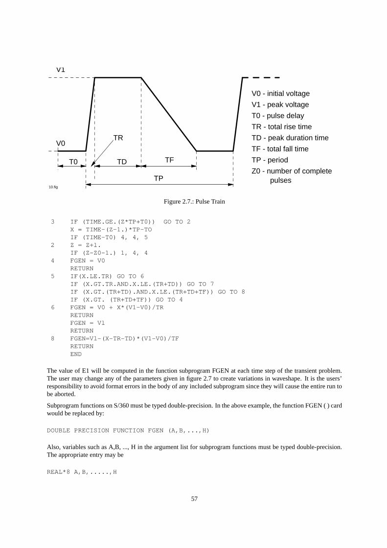
10.fig
V1
V0
T0 TD TF
TP
TR
V1 - peak voltage
T0 - pulse delay
TR - total rise time
TF - total fall time
TP - period
V0 - initial voltage
TD - peak duration time
Z0 - number of completepulses
Figure 2.7.: Pulse Train
3 IF (TIME.GE.(Z*TP+T0)) GO TO 2X = TIME-(Z-1.)*TP-TOIF (TIME-T0) 4, 4, 5
2 Z = Z+l.IF (Z-Z0-1.) 1, 4, 4
4 FGEN = V0RETURN
5 IF(X.LE.TR) GO TO 6IF (X.GT.TR.AND.X.LE.(TR+TD)) GO TO 7IF (X.GT.(TR+TD).AND.X.LE.(TR+TD+TF)) GO TO 8IF (X.GT. (TR+TD+TF)) GO TO 4
6 FGEN = V0 + X*(V1-V0)/TRRETURNFGEN = VlRETURN
8 FGEN=Vl-(X-TR-TD)*(V1-V0)/TFRETURNEND
The value of E1 will be computed in the function subprogram FGEN at each time step of the transient problem.The user may change any of the parameters given in figure 2.7 to create variations in waveshape. It is the users’responsibility to avoid format errors in the body of any included subprogram since they will cause the entire run tobe aborted.
Subprogram functions on S/360 must be typed double-precision. In the above example, the function FGEN ( ) cardwould be replaced by:
DOUBLE PRECISION FUNCTION FGEN (A,B,...,H)
Also, variables such as A,B, ..., H in the argument list for subprogram functions must be typed double-precision.The appropriate entry may be
REAL*8 A,B,.....,H
57

or
IMPLICIT REAL*8 (A-H)
2.7.1. Subprogram insertion
7090/94 only:
Once the subprogram cards are generated, they are inserted in the second half of the SCEPTRE Program ControlDeck behind the $IBJOB card PGMC1970 (see figure??). Assuming that a source deck is to be submitted, theproper sequence of cards would be
$IBJOB ALTIO,NOFLOW$IBFTC FGEN. FULIST,DECK
FUNCTION FGEN (V0, V1, T0, TR, TD, TF, TP, Z0, TIME)...........END
This feature may be used more efficiently by inserting the subprogram in compiled form. The compiled deck issimply inserted behind the second $IBJOB card, PGMC1970, as illustrated in figure??.
S/360 only:
When S/360 subprogram cards are generated, they are inserted in the second half of the SCEPTRE ProgramControl Deck behind the card identified as PGMC0310 in figure??. If, instead, an object deck is available it issimply inserted behind the card identified as PGMC0360.
This example was intended to build a General wave for input purposes. The imaginative user will find otherapplications in the course of practical analysis which cannot be implemented through conventional input.
2.7.2. Subprogram with models
There is no difficulty in combining the subprogram feature with stored models. The models may be stored (eitherpermanently or temporarily) with appropriate reference to the user’s subprograms. To illustrate:
MODEL DESCRIPTIONMODEL name (PERM) (1-6-4-A)ELEMENTSL2, 1-2 = FCOR (IL1, IL2, IL3, 25., 100.)...........
Here the user would ensure that the model includes elements L1, L2 and L3 because the currents through theseelements have been used as arguments in the subprogram. The subprogram itself should be supplied in eithersource or object form as in subsection 2.7.1.
2.8. Additional output and control
Some additional output and control is available to the interested user. This information will probably not be desiredfor most runs that are made but can be useful in special situations.
58

2.8.1. SIMUL8 program data
Normally, the program outputs the results of initial conditions computations once after convergence has beenachieved regardless of the number of iterations required. However, all resistor and primary dependent currentsource voltages may be output after each iteration of the DC program. In addition, all the formatted data that isused by the FORTRAN program (SIMUL8) written by SCEPTRE is available. This information may be obtainedby the request
WRITE SIMUL8 DATA
in the RUN CONTROLS section.
2.8.2. No element sort
In the absence of any user direction, the program forms the network tree by giving priority to the smaller elementswithin any passive element type. Variable elements are considered to have zero value for this purpose. If theinstruction
NO ELEMENT SORT
is inserted in the RUN CONTROLS section, tree priority is given within passive element types according to ordersof appearance under ELEMENTS. This instruction of course does not change the basic element type preferenceorder of E, C, R and L.
2.8.3. Matrix printouts
7090/94 only:
The network B matrix, which gives the topological relation between all network links and tree branches, is availablein labeled and constructed form. The required entry is BTFORM = 1 to obtain the matrix for the transient program.The corresponding matrix for the DC program is called by BTFORM=2. A card indicating the desired optionmust be placed immediately after the $DATA card that normally precedes MODEL DESCRIPTION or CIRCUITDESCRIPTION.
S/360 only:
The network B matrix, which gives the topological relation between all network link and tree branches, is availablein labeled and constructed form. To obtain the matrix for the transient program and/or DC program, the entry
PRINT B MATRIX
must be placed in the RUN CONTROLS section of the SCEPTRE input data.
2.8.4. Nodal listing
A printed listing of each network node and the elemente incident at the node can be generated with any run. (SeeAppendix A.6.) This listing is requested by
LIST NODE MAP
59

2.8.5. AC matrix outputs
Three Run Controls are provided to enable the interested user to obtain additional outputs relative to an AC analysis.The appropriate card formats as an indication of the outputted information are as follows:
PRINT A MATRIX
This output depends on the particular case involved. See [2, subsection 2.5] for an explanation of the four casesencountered.
For case (1) independent sources only, the output will be the system Matrices A and G.
For case (2) independent sources and dependent sources, the output will be the system Matrices A, G and H.
For case (3) independent sources requiring time derivatives, the output will be the system Matrices A, G, and Q.
For case (4) independent sources requiring time derivatives and dependent sources, the output will be the systemMatrices A, G, H and Q.
PRINT EIGENVALUES
This entry will result in a listing of the N complex valued eigenvalues obtained in the analysis. As a check onthe correctness of the similarity transformation, it will also cause a print-out of the results of the calculationΛS-SΛ, where S is the complex-valued modal matrix andΛ is the diagonal matrix composed of the complex systemeigenvalues. If the transformation is correct, the calculation gives the zero matrix.
PRINT EIGENVECTORS
This entry will result in a listing of the S matrix and the inverse of this matrix, S−1. As a check on the correctinessof the inversion it will also provide the results of the calculation S*S−1-1. If the matrix inversion is correctlyobtained, this calculation gives the zero matrix.
2.8.6. Program Debug Output
A program debug outputting facility which is provided principally as a program debugging aid is available to theinterested user. With this feature, data normally generated, used and of concern only internal to the program canbe printed out. In normal application of the program, this type of information is not desired and hence the facilityis not normally activated. To activate the debug printout feature request
WRITE DEBUG
in theRUN CONTROLSsection of the SCEPTRE input data.
2.9. Error diagnostics
The free form input data format of SCEPTRE is intended to minimize formatting errors. Other types of errors suchas those of omission, ambiguity, inconsistency, and violation (of syntax, program limits, etc.) must be detectedand diagnosed and the user alerted. For this purpose, the program possesses a comprehensive input data diagnosticcapability. A listing of the principal error messages in the input processor program are shown below. As the inputdata cards are read-in by the input processor, each card is printed-out and then scanned for errors. If an error isfound, an error message stating the trouble is printed immediately following the detection of the error. The severityof errors detected in this manner is also indicated. There are three levels of severity:
60

Level 1: (warning only) errors of this type are not critical and will be repaired by the input processor. The errorscan is continued and the analysis phase executed providing that errors of a higher level are not detectedelsewhere in the input data.
Level 2: (simulation deleted) errors of this type are critical and thus prohibit execution of the analysis phase.However, the error scan is continued in order to detect, diagnose and alert the user of any remaining errorsin the input data.
Level 3: (execution terminated) this type of error will not permit the. proper execution of the input processor and,thence successful continuation of either the error scan or execution of the analysis phase.
Most input data errors fall into level 2 as illustrated by the following example of an initial condition specificationwhich should contain an ’I’ prefix designating the initial current through inductor L3:
INITIAL CONDITIONSVC1 = 100L3 = 0.01
*** Error Message 1 - level 2 - simulation deleted - ERROR SCAN CONTINUESINITIAL CONDITION LACKS A ’V’ OR ’I’ PREFIX
Error messages
Messages numbered #2 and #3 are not issued in the System/360 version. Instead, the run will be aborted aftermessage #1 is issued and the system condition code set to terminate processing.
1 INITIAL CONDITION LACKS A ’V’ OR ’I’ PREFIX2 EQUAL SIGN MISSING3 VARIABLE NAME EXCEED CHARACTER LIMIT4 REDUNDANT VOLTAGE OR CURRENT SPECIFICATION5 NO VALUE SPECIFICATION FOLLOWS EQUALS6 INCORRECT VALUE SPECIFICATION7 MORE THAN 100 INITIAL CONDITIONS HAVE BEEN SPECIFIED8 THE MAXIMUM OF 100 DEFINED PARAMETERS HAS BEEN EXCEEDED9 DEFINED PARAMETER LACKS A ’D’ or ’P’ PREFIX
10 DEFINED PARAMETER DERIVATIVE CANNOT BE A CONSTANT11 IMPROPER DELIMITER SEQUENCE FOUND IN NODE STRING12 NODE DESIGNATION MISSING13 LIMIT OF 25 MODEL NODES HAS BEEN EXCEEDED14 NODE STRING IMPROPERLY TERMINATED15 PRECEDING MODEL IS NOT IN THE MODEL LIBRARY16 TABLE NAME OR INDEPENDENT VARIABLE EXCEEDS 6 CHARACTERS17 TABLE VALUE OR ARGUMENT EXCEEDS VALUE LIMIT18 TABLE INDEPENDENT VARIABLE IMPROPERLY SPECIFIED19 RIGHT PAREN FOLLOWING TABLE INDEPENDENT VARIABLE MISSING20 EQUATION ARGUMENT STRING MISSING21 NO OUTPUT REQUESTS SUPPLIED, RE-OUTPUT HAS BEEN DELETED22 INCORRECT DELIMITER OR INSUFFICIENT DATA ON CARD23 THE LIMIT OF ONE HUNDRED OUTPUTS HAS BEEN EXCEEDED24 MISSING COMMA SUPPLIED BY PROCESSOR
61

25 OUTPUT VARIABLE OR LABEL EXCEEDS SIX CHARACTERS26 PLOT NAME OR LABEL IS MISSING27 PRECEDING UNRECOGNIZABLE CARD IGNORED28 THE MAX OF 100 DEFINED PARAMETER DERIVATIVES IS EXCEEDED29 REDUNDANT DEFINED PARAMETER OR DEFINED PARAM DERIVATIVE30 MAX OF TEN TERMINATE IF RUN CONTROLS HAS BEEN EXCEEDED31 IMPROPER RUN CONTROL FORMAT32 INCOMPLETE SPECIFICATION PRIOR TO GROUP OR MODE CARD33 LEFT PAREN MISSING FOR TERMINATION CONTROL34 EXTRANEOUS DELIMITER IGNORED35 SECONDARY DEPENDENT SOURCE IMPROPERLY SPECIFIED36 INVALID NUMBER OR INTEGRATION ROUTINE37 UNRECOGNIZABLE DATA FOLLOWS MODEL DESCRIPTION38 MODEL NAME MISSING39 REDUNDANT MODEL HAS BEEN SPECIFIED40 THE MAXIMUM OF 11 HEADING CARDS HAS BEEN EXCEEDED41 TABLE OR EQUATION SPECIFICATION EXPECTED42 INCOMPLETE EQUATION OR UNEVEN TABLE PRIOR TO NEW FUNCTION43 TABLE OR EQUATION IMPROPERLY SPECIFIED44 TABLE OR EQUATION IS REDUNDANT45 TABLE OR EQUATION NAME EXCEEDS SIX CHARACTERS46 INVALID CONSTANT SPECIFIED47 TABLE DATA EXCEEDS CAPACITIY OF THE INPUT PROCESSOR48 THE MAXIMUM OF 300 ELEMENTS HAS BEEN EXCEEDED49 THE MAXIMUM OF 50 MUTUAL INDUCTANCES HAS BEEN EXCEEDED50 THE MAXIMUM OF 50 SOURCE DERIVATIVES HAS BEEN EXCEEDED51 COMMA OR = SIGN MISSING OR WRONG DERIVATIVE SPECIFIED52 SOURCE ELEMENT MISSING FOR TABLE OR DIODE EQUATION53 INCORRECT MODEL CARD - ELEMENT NAME INCOMPLETE54 IMPROPER MODEL CHANGE SPECIFIED55 INCONSISTENT MODEL CHANGE, EQUATION AND TABLE ARE EQUATED56 LIMIT OF 15 TABLE OR EQUATION MODEL CHANGES EXCEEDED57 INSUFFICIENT MODEL NODES SPECIFIED58 MODEL NAME EXCEEDS EIGHTEEN CHARACTERS59 MODEL CIRCUIT DESIGNATION EXCEEDS FOUR CHARACTERS60 MODEL CHANGE VALUE IS VARIABLE61 THE LIMIT OF TEN SUPPRESSED OUTPUTS HAS BEEN EXCEEDED62 UNRECOGNIZABLE MODEL MODIFICATION DATA63 MORE THAN 250 TEMPORARY OR PERMANENT MODELS SPECIFIED64 AN EQUATION IS NOT A PERMISSABLE ARGUMENT65 IMPROPER ARGUMENT FORMAT66 EQUATION, ARGUMENT OR VALUE EXCEEDS 1200 CHARACTERS67 MODEL NOT IN SPECIFIED LIBRARY, ALTERNATE LIB SCAN STARTS68 MUTUAL INDUCTANCE REFERENCES NON-EXISTENT INDUCTOR69 SOURCE DERIVATIVE REFERENCES NON-EXISTENT SOURCE70 DEFINED PARAM DERIV. REFERENCES NON-EXISTENT DEF. PARAM.71 A MODEL ELEMENT CANNOT BE A MODEL72 ELEMENT, MUTUAL INDUCTANCE OR SOURCE DERIV IS REDUNDANT73 MODEL TABLE OR EQUATION CHANGE IS REDUNDANT74 ELEMENT IMROPERLY SPECIFIED75 REFERENCED TABLE, EQUATION, DEF PARAM OR ELEMENT MISSING76 THE FOLLOWING OUTPUT REQUEST IS NOT VALID
62

77 NO OUTPUT REQUESTS HAVE BEEN SUPPLIED78 IMPROPER EXPRESSION FORMAT --COMPUTATION DELAYS MAY OCCUR79 INVALID SYNTAX80 TABLE XXX FORMAT ALTERED TO TXXX81 TIME SUPPLIED AS ARGUMENT IN XTABLE FUNCTION82 THE MAX. OF 100 PARTIAL DFPRAM. DERIV. HAS BEEN EXCEEDED83 PART. DFPRAM DERIV REFERENCES NON-EXISTENT DFPRAM DERIV.84 INVALID OR MISSING DELIMITER IN A DC OPTION CARD85 INVALID VARIABLE IN A DC OPTION CARD86 MONTE CARLO DEFAULT, 10 PASSES SUPPLIED87 OPTIMIZATION DEFAULT, 30 PASSES SUPPLIED88 NOMINAL VALUE DOES NOT LIE BETWEEN BOUNDS89 AC RUN REQUESTED WITH INITIAL CONDITIONS ONLY RUN90 COMPLEX DEFINED PARAMETER GIVEN AS REAL CONSTANT91 LIMIT OF 50 COMPLEX DEFINED PARAMETERS EXCEEDED92 AC SOURCES PRESENT IN NON-AC RUN93 SYMBOLIC JACOBIAN WITH ADJOINT RUN MAY LEAD TO ERROR94 INVALID OR MISSING DELIMITER IN A DIFFERENTIAL DATA CARD95 INVALID VARIABLE IN A DIFFERENTIAL DATA CARD
The program generator portion of the program also contains a diagnostic capability to inform the user of errorsthat can only be detected after the network topology is analyzed. Such errors may or may not cause the executionof the analysis phase to be aborted as indicated by the error messages which occur. A list of diagnostic messagesthat may originate in the program generator follows.
AN ILLEGAL PROCESSING SEQUENCE HAS BEEN REQUESTEDPROGRAM CAPACITY HAS BEEN EXCEEDED--XXX LIST OVER FLOWED IN FILING XXX’WTSPTP’ HAS BEEN ASKED TO WRITE XXX SOURCE STATEMENT CARDS.
THE LIMIT is xxxTHE IIIIII ELEMENTS TO BE PROCESSED EXCEEDS THE LIMIT OF XXX.XXX RESULTS IN A CURRENT SOURCE CUT SET.XXX CAUSES J-C CUT SET PREVENTING I/C SOLUTION.XXX RESULTS IN A VOLTAGE SOURCE LOOP.XXX CAUSES E-L LOOP PREVENTING I/C SOLUTION.THE ELEMENT XXX FROM XXX TO XXX IS SHORTED OUT OF TRE CIRCUIT.
EXECUTION WILL BE TERMINATED AFTER COMPLETED ERROR SCAN.WARNING ONLY -- THE XXX NODE OF XXX IS NOT CONNECTED TO ANY OTHER
ELEMENT IN THE CIRCUIT -- EXECUTION CONTINUES.AN ERRONEOUS TREE BRANCH EXISTS IN THE PATH OF XXX.ERROR IN BCD CONVERSION OF XXX ENTRIES IS CLASS IITHE REFERENCE INDUCTOR XXX FOR XXX CANNOT BE FOUND IN THE ELEMENTS TABLEPROGRAM ERROR IN ’WTEQTN’. ILLEGAL ARGUMENT TYPE CODE FOUND IN DEPENDENCY
TABLE.THE VARIABLE XXX COULD NOT BE FOUND IN THE VALUE LIST BY ’WTEQTN’ - PROGRAM
ERROR.THE VARIABLE XXX IS DEPENDENT UPON ITSELF. THE RUN CANNOT BE CONTINUED.THE DEPENDENCY TABLE HAS OVERFLOWED IN ’WTEQTN’ - PROGRAM ERROR.THE TERM XXX WILL CAUSE A COMPUTATIONAL DELAY.THE TERM XXX COULD NOT BE FOUND IN THE VALUE LIST BY ’EQFORM’ - PROGRAM ERROR.VALUE EXPRESSION FOR TYPE 6 IS NOT CODED YET. THE RUN CANNOT BE CONTINUED.THE VARIABLE XXX CANNOT BE FOUND IN EITHER THE LIST OF CIRCUIT ELEMENTS
OR DEFINED PARAMETERS BY ’COMPCK’.
63

THE FOLLOWING INVALID PREFIX HAS BEEN SUPPLIED TO ’COPYDP’, ’X’’COPYDP’ IS BEING REQUESTED TO GENERATE THE FOLLOWING (INVALID) RESISTOR
DERIVATIVE TERM IN AN EQUATION XXXTHE FOLLOWING TERM WILL CAUSE THE DEPENDENCY TABLE TO OVERFLOW XXX’SCANEQ’ COULD NOT FIND THE TERM XXX IN THE ELEMENTS TABLE -- PROGRAM ERRORTHE XXX ELEMENT COMPLETES A LOOP CONTAINING XXX WHICH WILL PROHIBIT AN
INITIAL CONDITIONS SOLUTION.THE VARIABLE ELEMENT (XXX) COMPLETES A LOOP CONTAINING AN ELEMENT OF THE
SAME TYPE WHICH PROHIBITS AN IC SOLUTIONCAPACITOR XXX REFERENCED IN TABLE OR EQUATION BUT NOT SUPPLIED AS ELEMENTELEMENT XXX IS FUNCTION OF CAPACITOR XXX VOLTAGE FOR WHICH VOLTAGE
SUBSTITUTION CANNOT BE PERFORMED (INITIAL CONDITIONS)RESISTOR OR INDUCTOR CURRENT SUPPLIED AS TABLE INDEPENDENT VARIABLE OR
EQUATION ARGUMENT FOR XXX IS NOT ALLOWED FOR INITIAL CONDITIONS PROBLEMXXX UPON WHICH XXX IS DEPENDENT CANNOT BE FOUND IN THE CLASS 9 SECTION
OF THE ELEMENTS TABLE.AN INTEGER-TO-BCD CONVERSION ERROR OCCURRED IN A DIMENSION STATEMENT GENERATIONXXX WHICH XXX IS DEPENDENT UPON IS NOT IN THE CLASS 2 OR 5 SECTION OF
ELEMENTS--PROGRAM ERRORTHE VMUTUAL SUBROUTINE SUPPLIED XXX FOR TYPE OF MUTUAL TERM TO BE ADDED
TO V3P(N) or V6(N)--MUST BE IN RANGE OF 1 - 5.THE DERIVATIVE OF THE VARIABLE SOURCE XXX HAS NOT BEEN SUPPLIED.’GTCODE’ CAN’T ENCODE THE ILLEGAL TERM XXX - PROGRAM ERROR.NUMBER OF HEADING CARDS EXCEEDS MAXIMUM - THIS CARD IS IGNOREDSIMUL8 DATA GENERATION HAS BEEN DELETED FOR THIS RERUNNO STOP TIME HAS BEEN SPECIFIEDILLEGAL INITIAL CONDITION VARIABLE NAME - XXXIMPROPER VALUE SPECIFICATION ON CARD PRIOR TO GROUP CARDILLEGAL VALUE SPECIFICATIONILLEGAL TABLE SPECIFICATIONEXTRANEOUS X IGNOREDFOLLOWING VARIABLE NAME TRUNCATED TO SIX CHARACTERS XXX -----INCORRECT DELIMITER FOLLOWS VARIABLE NAME XXXXXX AN = HAS BEEN SUPPLIEDINCORRECT DELIMITER FOLLOWS VARIABLE VALUE EEEEEEE. EEEEE X, HAS BEEN SUPPLIEDILLEGAL RUN CONTROL SPECIFICATIONRUN CONTROL DATA MISSINGINITIAL CONDITIONS WERE NOT SPECIFIED FOR THE ORIGINAL RUNEXTRANEOUS X IGNOREDINCORRECT DELIMITER FOR FOLLOWING RUN CONTROL SPECIFICATION XXXAN EQUAL SIGN HAS BEEN SUPPLIEDINVALID NUMBER OR INTEGRATION ROUTINE SPECIFIEDNO ENTRIES IN RERUN DATA LISTILLEGAL VARIABLE NAME - XXXILLEGAL TABLE NAME SPECIFICATION - XXXTABLE XXX - RERUN TABLE EXCEEDS LENGTH OF ORIGINAL TABLEILLEGAL CONTINUE SPECIFICATIONILLEGAL RUN CONTROL SPECIFICATIONRUN CONTROL DATA MISSINGINCOMPLETE RUN CONTROL SPECIFICATION ON CARD PRIOR TO END CARDILLEGAL DEBUG CARD IGNOREDTHE NEWTON-RAPHSON PASS LIMIT HAS BEEN EXCEEDED WITHOUT ATTAINING CONVERGENCEMATRIX XXX IS SINGULAR
64

UNABLE TO LOCATE DEPENDENT PLOT VARIABLE FOR INDEPENDENT VARIABLE XXXNO. PLOT PTS. HAVE EXCEEDED PLOT STORAGE BLOCK SIZEDERIVATIVE XXX FOUND IN THE TERMINATION CONDITION(S) IS NOT RESOLVEDTHE LENGTH OF THE FIRST SOLUTION BUFFER IS ZERO.MORE THAN 9 OUTPUTS WERE REQUESTED ON PLOT NUMBER XXX. ONLY THE FIRST 9
REQUESTS WILL BE HONORED.PLOT REQUEST XXX WAS NOT SPECIFIED AS AN OUTPUT IN THE ORIGINAL (CIRCUIT
DESCRIPTION) RUN FOR THIS SYSTEM.MAXIMUM PLOT LENGTH (2000 LINES) HAS BEEN EXCEEDED.A TRACE ON ONE OF THE PLOTS IS DISPLACED FROM ZERO BY MORE THAN 10**6 TIMES
ITS TOTAL RANGE. LOSS OF SIGNIFICANCE IS POSSIBLE IN THESE RESULTS.TABLE CONTAINING IMPLICIT INTEGRATION DATA HAS OVERFLOWED. SIMULATION
HAS BEEN DELETED.TABLE CONTAINING SPARSE MATRIX DATA HAS OVERFLOWED. SIMULATION HAS BEEN
DELETED.TABLES CONTAINING SPARSE MATRIX DATA HAVE OVERFLOWED. PIVOTING OF THE
MATRIX WILL BE DELETED.
7090/94 only:
If the analysis phase is aborted by any of the error messages indicated above, the following messages will alsoappear.
IBFTC CARD WITH CORRECT DECK NAME NOT FOUND.
This message is printed following the Program Control Deck card labeled PGMC 1960.
LOADING HAS BEEN SUPPRESSED.
This message is printed following PGMC 2300.
65
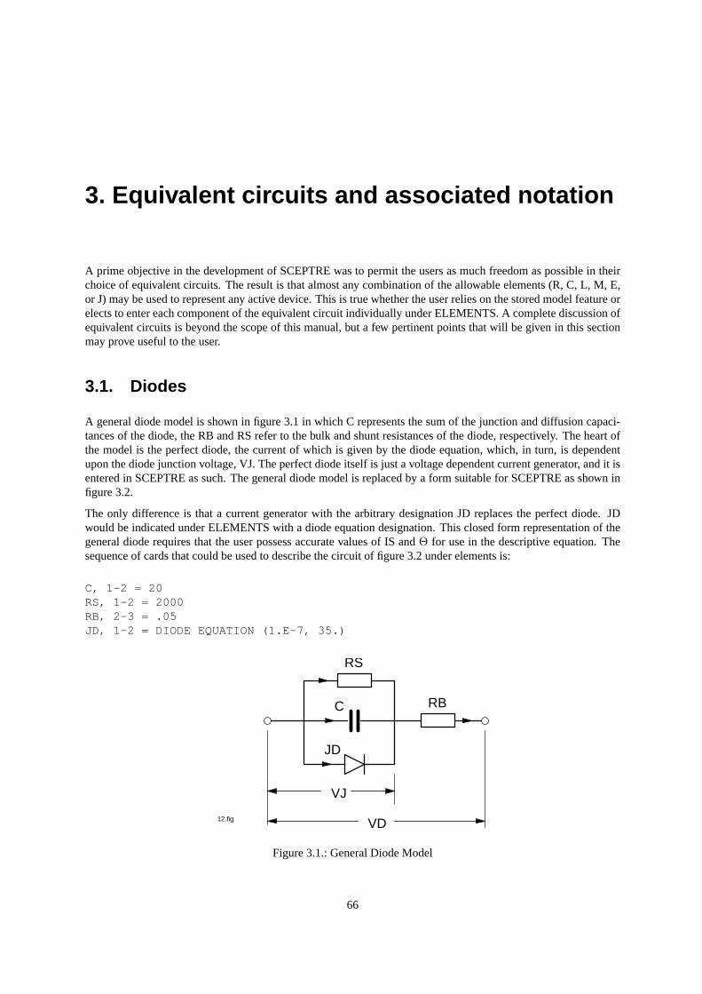
3. Equivalent circuits and associated notation
A prime objective in the development of SCEPTRE was to permit the users as much freedom as possible in theirchoice of equivalent circuits. The result is that almost any combination of the allowable elements (R, C, L, M, E,or J) may be used to represent any active device. This is true whether the user relies on the stored model feature orelects to enter each component of the equivalent circuit individually under ELEMENTS. A complete discussion ofequivalent circuits is beyond the scope of this manual, but a few pertinent points that will be given in this sectionmay prove useful to the user.
3.1. Diodes
A general diode model is shown in figure 3.1 in which C represents the sum of the junction and diffusion capaci-tances of the diode, the RB and RS refer to the bulk and shunt resistances of the diode, respectively. The heart ofthe model is the perfect diode, the current of which is given by the diode equation, which, in turn, is dependentupon the diode junction voltage, VJ. The perfect diode itself is just a voltage dependent current generator, and it isentered in SCEPTRE as such. The general diode model is replaced by a form suitable for SCEPTRE as shown infigure 3.2.
The only difference is that a current generator with the arbitrary designation JD replaces the perfect diode. JDwould be indicated under ELEMENTS with a diode equation designation. This closed form representation of thegeneral diode requires that the user possess accurate values of IS andΘ for use in the descriptive equation. Thesequence of cards that could be used to describe the circuit of figure 3.2 under elements is:
C, 1-2 = 20RS, 1-2 = 2000RB, 2-3 = .05JD, 1-2 = DIODE EQUATION (1.E-7, 35.)
VJ
VD
C
RS
RB
JD
12.fig
Figure 3.1.: General Diode Model
66
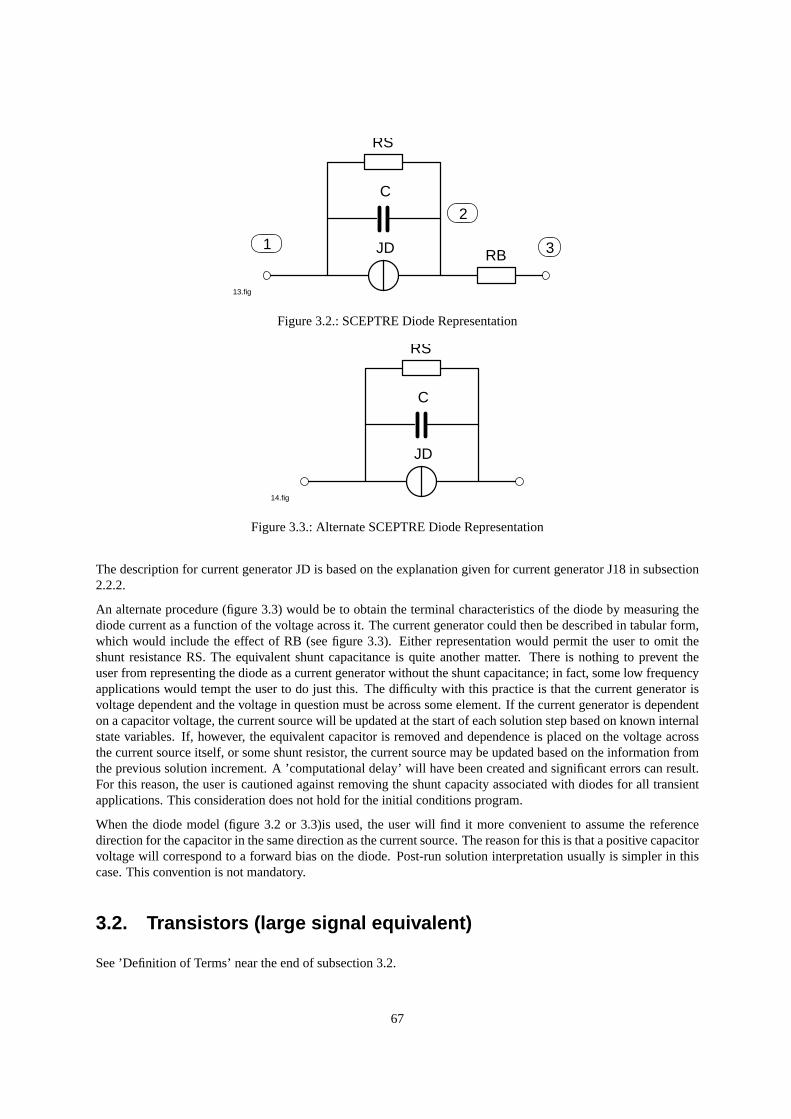
13.fig
1
2
3
RS
C
JD RB
Figure 3.2.: SCEPTRE Diode Representation
RS
C
JD
14.fig
Figure 3.3.: Alternate SCEPTRE Diode Representation
The description for current generator JD is based on the explanation given for current generator J18 in subsection2.2.2.
An alternate procedure (figure 3.3) would be to obtain the terminal characteristics of the diode by measuring thediode current as a function of the voltage across it. The current generator could then be described in tabular form,which would include the effect of RB (see figure 3.3). Either representation would permit the user to omit theshunt resistance RS. The equivalent shunt capacitance is quite another matter. There is nothing to prevent theuser from representing the diode as a current generator without the shunt capacitance; in fact, some low frequencyapplications would tempt the user to do just this. The difficulty with this practice is that the current generator isvoltage dependent and the voltage in question must be across some element. If the current generator is dependenton a capacitor voltage, the current source will be updated at the start of each solution step based on known internalstate variables. If, however, the equivalent capacitor is removed and dependence is placed on the voltage acrossthe current source itself, or some shunt resistor, the current source may be updated based on the information fromthe previous solution increment. A ’computational delay’ will have been created and significant errors can result.For this reason, the user is cautioned against removing the shunt capacity associated with diodes for all transientapplications. This consideration does not hold for the initial conditions program.
When the diode model (figure 3.2 or 3.3)is used, the user will find it more convenient to assume the referencedirection for the capacitor in the same direction as the current source. The reason for this is that a positive capacitorvoltage will correspond to a forward bias on the diode. Post-run solution interpretation usually is simpler in thiscase. This convention is not mandatory.
3.2. Transistors (large signal equivalent)
See ’Definition of Terms’ near the end of subsection 3.2.
67
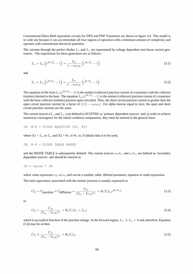
Conventional Ebers-Moll equivalent circuits for NPN and PNP Transistors are shown in figure 3.4. This model isin wide use because it can accommodate all four regions of operation with a minimum amount of complexity andoperates with conventional electrical quantities.
The currents through the perfect diodesIre andIrc are represented by voltage dependent non-linear current gen-erators . The expressions for these generators are as follows:
Ire = Ies
(eΘeV
′be − 1
)=
Ieo1− αIαN
(eΘeV
′be − 1
)(3.1)
and
Irc = Ics
(eΘcV
′bc − 1
)=
Ico1− αIαN
(eΘcV
′bc − 1
)(3.2)
The equation of the formIxs(eΘxVbx−1) is the emitter (collector) junction current of a transistor with the collector(emitter) shorted to the base. The equationIxo(eΘxVbx−1) is the emitter (collector) junction current of a transistorwith the base-collector (emitter) junction open-circuited. Thus, the short circuit junction current is greater than theopen circuit junction current by a factor of1/(1 − αIαN ). For alpha inverse equal to zero, the open and shortcircuit junction currents are the same.
The current sources (Ire andIrc ) are defined in SCEPTRE as ’primary dependent sources’ and, in order to achievenumerical convergence for the initial condition computation, they must be entered in the general form:
JX, B-X = DIODE EQUATION (X1, X2)
where X1 =Ies or Ics and X2 =Θe or Θc or, if tabular data is to be used,
JB, B-X = DIODE TABLE XXXXX
and the DIODE TABLE is subsequently defined. The current sourcesαNIre andαIIrc are defined as ’secondarydependent sources’ and should be entered as
JS = value * JX
where value representsαN or αI and can be a number, table, defined parameter, equation or math expression.
The total capacitance associated with the emitter junction is usually expressed as
CE = Cjunction+ Cdiffusion =Coe
(Voe − VCE)ne+ ΘeTeIese
ΘeVCE (3.3)
or
CE =Coe
(Voe − VCE)ne+ ΘeTe(Ire + Ies) (3.4)
which is an explicit function of the junction voltage. In the forward region,Ire Ies > 0 and, therefore, Equation(3.4) may be written
CE ≈Coe
(Voe − VCE)ne+ ΘeTeIre (3.5)
68
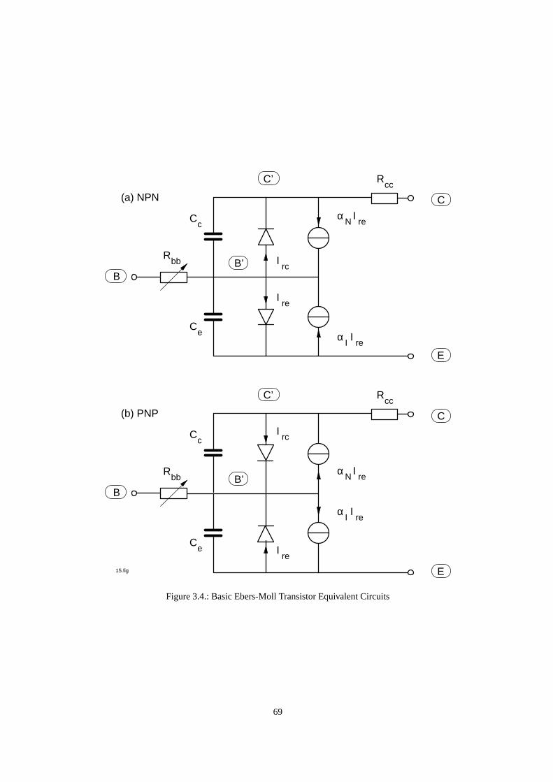
Irc
α IreN
αII
re
Ire
R
C
E
B’R
bb
C
C’cc
c
eC
B
15.fig
R
C
E
B’R
bb
C
C’
I
α
cc
IreNc
rc
αII
re
Ire
eC
B
(a) NPN
(b) PNP
Figure 3.4.: Basic Ebers-Moll Transistor Equivalent Circuits
69
Note that Equation (3.4) must always have a positive diffusion capacitance, even whenIre < 0 (because|Ies| >|Ire|whenVCE < 0 in the diode equation), but that a negative diffusion capacitance and, therefore, a negative totalcapacitance is conceivable in (3.5). Normally, any negative contribution due to the diffusion term will be ordersof magnitude less than the positive junction term and the total capacitance will be positive. It is clear that, if thecurrent sourceIre in (3.5) is represented by a diode table that permits no negative current, a negative capacitanceis never possible. The situation regarding the collector capacitance is not substantially different as (3.4) becomes
CC =Coe
(Voc − VCC)nc+ ΘcTs(Irc + Ics) (3.6)
In SCEPTRE language, the total emitter capacitance may be entered as
CE, B-X EQUATION 1 (K1, K2, VCE, K3, K4, JE, K5)
and
EQUATION 1 (A, B, C, D, E, F, G) = (A/(B-C)** D + E*(F+G))
where the constants have been chosen as
K1 = Coe K2 = Voe K3 = ne K4 = ΘeTe K5 = Ies
If JE is in a tabular form that insures JE≥ 0 only, or if the user is confident that his application cannot cause anegative capacitance, a reasonable simplification permits the entry
CE, B-X = EQUATION 2 (K1, K2, VCE, K3, K4, JE)
and
EQUATION 2 (A, B, C, D, E, F) = (A/(B-C)**D + E* F)
A popularly used approximation is to consider that the junction component of capacitance is constant at some valueK6 . Then EQUATION 2 simplifies to
CE, B-X = EQUATION 3 (K6, K4, JE)
and
EQUATION 3 (A, B, C) = (A+B*C)
Another approximation that is often made is to enter RBB as a constant resistor when it really is a nonlinearfunction of emitter current. If the user desires a greater degree of sophistication in his model, any of the aboveconstants K1 – K6 may be entered as a variable quantity in equation or tabular form. The situation for the totalcollector capacitance is entirely analogous. The following examples illustrate suggested NPN and PNP transistormodels coded for SCEPTRE when closed form expressions forIre, Irc and the junction capacitances are available(Reference figure 3.5).
For the NPN:
70
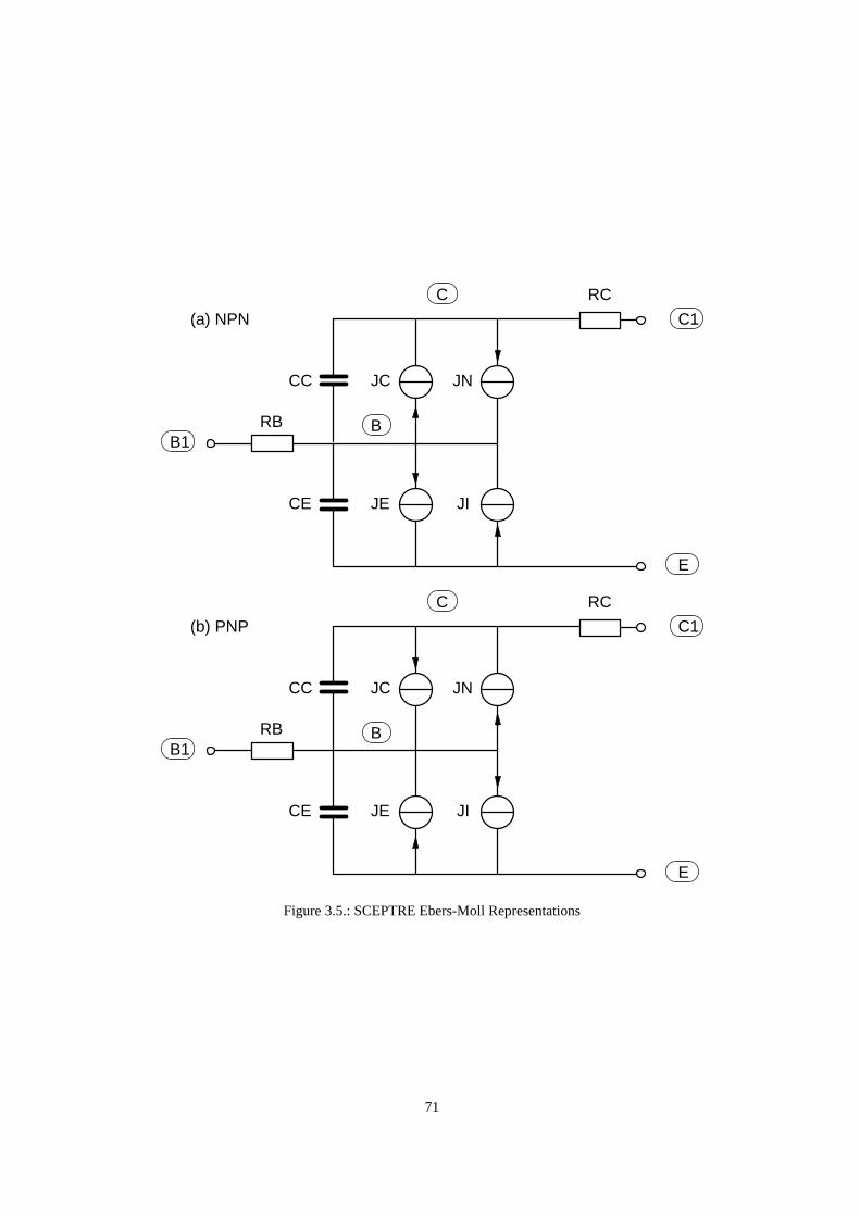
(a) NPN
B1
C
C1
E
B
CC
RB
JC JN
JIJECE
RC
B1
C
C1
E
B
CC
RB
JC JN
JIJECE
RC
(b) PNP
Figure 3.5.: SCEPTRE Ebers-Moll Representations
71
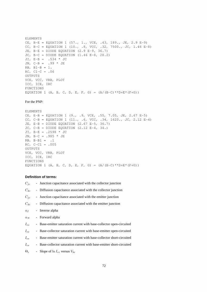
ELEMENTSCE, B-E = EQUATION 1 (57., 1., VCE, .43, 189., JE, 2.9 E-9)CC, B-C = EQUATION 1 (10., .8, VCC, .32, 7500., JC, 1.46 E-8)JE, B-E = DIODE EQUATION (2.9 E-9, 36.7)JC, B-C = DIODE EQUATION (1.46 E-8, 28.2)JI, E-B = .534 * JCJN, C-B = .99 * JERB, B1-B = 1.RC, C1-C = .06OUTPUTSVCE, VCC, VRB, PLOTICC, ICE, IRCFUNCTIONSEQUATION 1 (A, B, C, D, E, F, G) = (A/(B-C)**D+E*(F+G))
For the PNP:
ELEMENTSCE, E-B = EQUATION 1 (9., .9, VCE, .55, 7.05, JE, 2.67 E-5)CC, C-B = EQUATION 1 (11., .6, VCC, .34, 1620., JC, 2.12 E-4)JE, E-B = DIODE EQUATION (2.67 E-5, 36.7)JC, C-B = DIODE EQUATION (2.12 E-4, 34.)JI, B-E = .2598 * JCJN, B-C = .985 * JERB, B-B1 = .1RC, C-C1 = .005OUTPUTSVCE, VCC, VRB, PLOTICC, ICE, IRCFUNCTIONSEQUATION 1 (A, B, C, D, E, F, G) = (A/(B-C)**D+E*(F+G))
Definition of terms:
Cjc - Junction capacitance associated with the collector junction
Cdc - Diffusion capacitance associated with the collector junction
Cje - Junction capacitance associated with the emitter junction
Cde - Diffusion capacitance associated with the emitter junction
αI - Inverse alpha
αN - Forward alpha
Ieo - Base-emitter saturation current with base-collector open-circuited
Ico - Base-collector saturation current with base-emitter open-circuited
Ies - Base-emitter saturation current with base-collector short-circuited
Ics - Base-collector saturation current with base-emitter short-circuited
Θe - Slope ofln Ire versusVbe
72
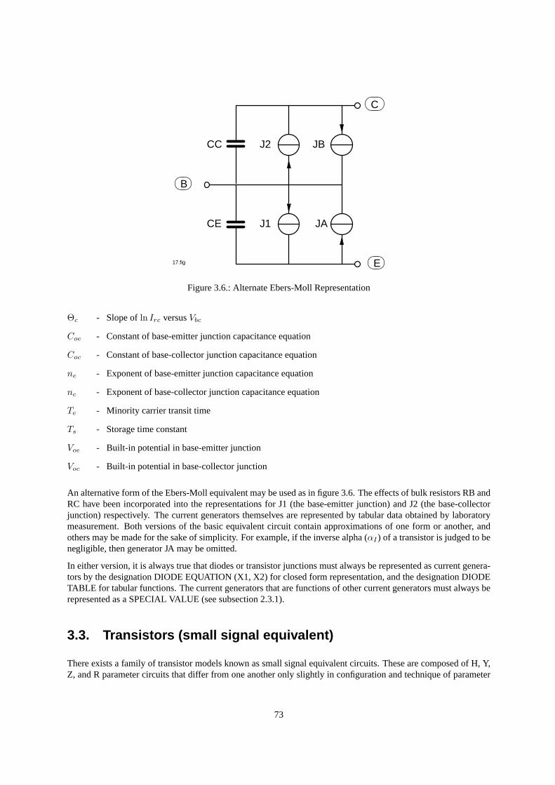
CC
CE
B
C
J1
J2 JB
JA
E17.fig
Figure 3.6.: Alternate Ebers-Moll Representation
Θc - Slope ofln Irc versusVbc
Coe - Constant of base-emitter junction capacitance equation
Coc - Constant of base-collector junction capacitance equation
ne - Exponent of base-emitter junction capacitance equation
nc - Exponent of base-collector junction capacitance equation
Te - Minority carrier transit time
Ts - Storage time constant
Voe - Built-in potential in base-emitter junction
Voc - Built-in potential in base-collector junction
An alternative form of the Ebers-Moll equivalent may be used as in figure 3.6. The effects of bulk resistors RB andRC have been incorporated into the representations for J1 (the base-emitter junction) and J2 (the base-collectorjunction) respectively. The current generators themselves are represented by tabular data obtained by laboratorymeasurement. Both versions of the basic equivalent circuit contain approximations of one form or another, andothers may be made for the sake of simplicity. For example, if the inverse alpha (αI ) of a transistor is judged to benegligible, then generator JA may be omitted.
In either version, it is always true that diodes or transistor junctions must always be represented as current genera-tors by the designation DIODE EQUATION (X1, X2) for closed form representation, and the designation DIODETABLE for tabular functions. The current generators that are functions of other current generators must always berepresented as a SPECIAL VALUE (see subsection 2.3.1).
3.3. Transistors (small signal equivalent)
There exists a family of transistor models known as small signal equivalent circuits. These are composed of H, Y,Z, and R parameter circuits that differ from one another only slightly in configuration and technique of parameter
73
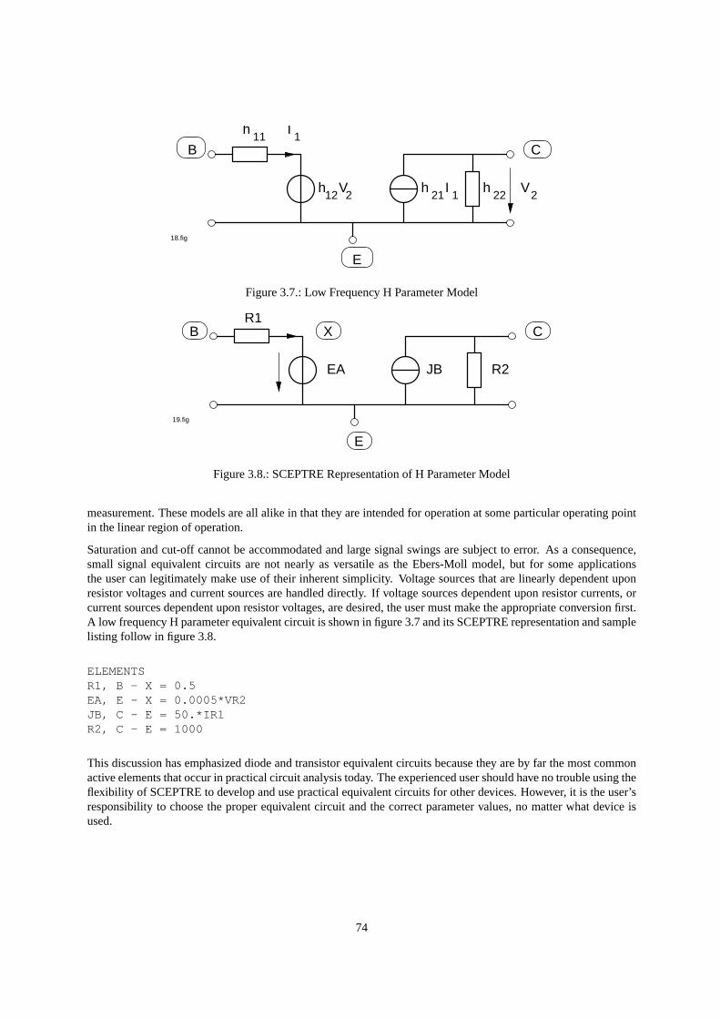
18.fig
B
h
E
C11
I1
h12
V2
h22
h21 1
I V2
Figure 3.7.: Low Frequency H Parameter Model
B C
19.fig
XR1
R2JBEA
E
Figure 3.8.: SCEPTRE Representation of H Parameter Model
measurement. These models are all alike in that they are intended for operation at some particular operating pointin the linear region of operation.
Saturation and cut-off cannot be accommodated and large signal swings are subject to error. As a consequence,small signal equivalent circuits are not nearly as versatile as the Ebers-Moll model, but for some applicationsthe user can legitimately make use of their inherent simplicity. Voltage sources that are linearly dependent uponresistor voltages and current sources are handled directly. If voltage sources dependent upon resistor currents, orcurrent sources dependent upon resistor voltages, are desired, the user must make the appropriate conversion first.A low frequency H parameter equivalent circuit is shown in figure 3.7 and its SCEPTRE representation and samplelisting follow in figure 3.8.
ELEMENTSR1, B - X = 0.5EA, E - X = 0.0005*VR2JB, C - E = 50.*IR1R2, C - E = 1000
This discussion has emphasized diode and transistor equivalent circuits because they are by far the most commonactive elements that occur in practical circuit analysis today. The experienced user should have no trouble using theflexibility of SCEPTRE to develop and use practical equivalent circuits for other devices. However, it is the user’sresponsibility to choose the proper equivalent circuit and the correct parameter values, no matter what device isused.
74
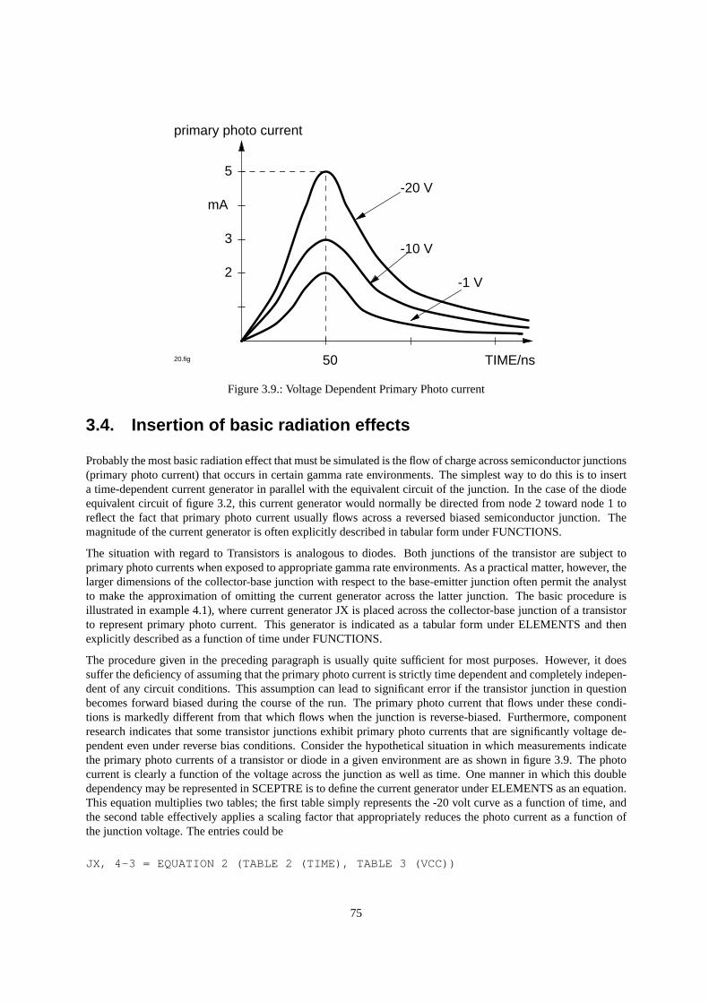
5
50
-20 V
-10 V
-1 V2
3
mA
TIME/ns
primary photo current
20.fig
Figure 3.9.: Voltage Dependent Primary Photo current
3.4. Insertion of basic radiation effects
Probably the most basic radiation effect that must be simulated is the flow of charge across semiconductor junctions(primary photo current) that occurs in certain gamma rate environments. The simplest way to do this is to inserta time-dependent current generator in parallel with the equivalent circuit of the junction. In the case of the diodeequivalent circuit of figure 3.2, this current generator would normally be directed from node 2 toward node 1 toreflect the fact that primary photo current usually flows across a reversed biased semiconductor junction. Themagnitude of the current generator is often explicitly described in tabular form under FUNCTIONS.
The situation with regard to Transistors is analogous to diodes. Both junctions of the transistor are subject toprimary photo currents when exposed to appropriate gamma rate environments. As a practical matter, however, thelarger dimensions of the collector-base junction with respect to the base-emitter junction often permit the analystto make the approximation of omitting the current generator across the latter junction. The basic procedure isillustrated in example 4.1), where current generator JX is placed across the collector-base junction of a transistorto represent primary photo current. This generator is indicated as a tabular form under ELEMENTS and thenexplicitly described as a function of time under FUNCTIONS.
The procedure given in the preceding paragraph is usually quite sufficient for most purposes. However, it doessuffer the deficiency of assuming that the primary photo current is strictly time dependent and completely indepen-dent of any circuit conditions. This assumption can lead to significant error if the transistor junction in questionbecomes forward biased during the course of the run. The primary photo current that flows under these condi-tions is markedly different from that which flows when the junction is reverse-biased. Furthermore, componentresearch indicates that some transistor junctions exhibit primary photo currents that are significantly voltage de-pendent even under reverse bias conditions. Consider the hypothetical situation in which measurements indicatethe primary photo currents of a transistor or diode in a given environment are as shown in figure 3.9. The photocurrent is clearly a function of the voltage across the junction as well as time. One manner in which this doubledependency may be represented in SCEPTRE is to define the current generator under ELEMENTS as an equation.This equation multiplies two tables; the first table simply represents the -20 volt curve as a function of time, andthe second table effectively applies a scaling factor that appropriately reduces the photo current as a function ofthe junction voltage. The entries could be
JX, 4-3 = EQUATION 2 (TABLE 2 (TIME), TABLE 3 (VCC))
75
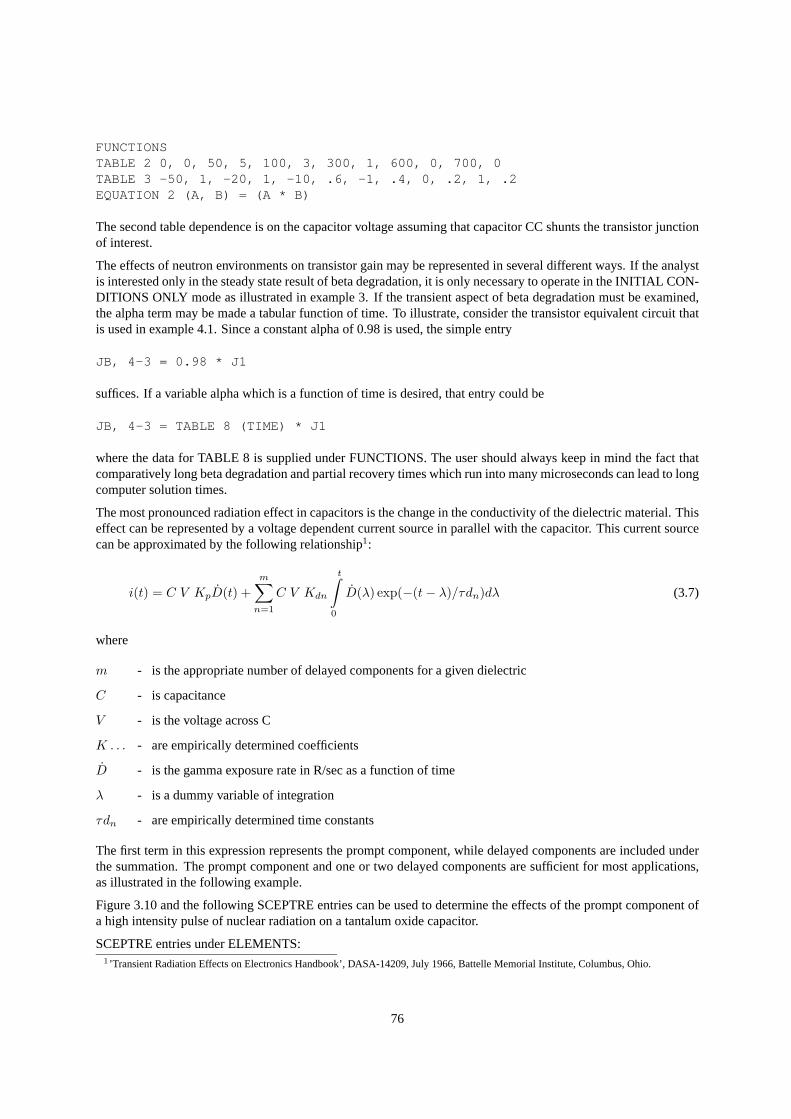
FUNCTIONSTABLE 2 0, 0, 50, 5, 100, 3, 300, 1, 600, 0, 700, 0TABLE 3 -50, 1, -20, 1, -10, .6, -1, .4, 0, .2, 1, .2EQUATION 2 (A, B) = (A * B)
The second table dependence is on the capacitor voltage assuming that capacitor CC shunts the transistor junctionof interest.
The effects of neutron environments on transistor gain may be represented in several different ways. If the analystis interested only in the steady state result of beta degradation, it is only necessary to operate in the INITIAL CON-DITIONS ONLY mode as illustrated in example 3. If the transient aspect of beta degradation must be examined,the alpha term may be made a tabular function of time. To illustrate, consider the transistor equivalent circuit thatis used in example 4.1. Since a constant alpha of 0.98 is used, the simple entry
JB, 4-3 = 0.98 * J1
suffices. If a variable alpha which is a function of time is desired, that entry could be
JB, 4-3 = TABLE 8 (TIME) * J1
where the data for TABLE 8 is supplied under FUNCTIONS. The user should always keep in mind the fact thatcomparatively long beta degradation and partial recovery times which run into many microseconds can lead to longcomputer solution times.
The most pronounced radiation effect in capacitors is the change in the conductivity of the dielectric material. Thiseffect can be represented by a voltage dependent current source in parallel with the capacitor. This current sourcecan be approximated by the following relationship1:
i(t) = C V KpD(t) +m∑n=1
C V Kdn
t∫0
D(λ) exp(−(t− λ)/τdn)dλ (3.7)
where
m - is the appropriate number of delayed components for a given dielectric
C - is capacitance
V - is the voltage across C
K . . . - are empirically determined coefficients
D - is the gamma exposure rate in R/sec as a function of time
λ - is a dummy variable of integration
τdn - are empirically determined time constants
The first term in this expression represents the prompt component, while delayed components are included underthe summation. The prompt component and one or two delayed components are sufficient for most applications,as illustrated in the following example.
Figure 3.10 and the following SCEPTRE entries can be used to determine the effects of the prompt component ofa high intensity pulse of nuclear radiation on a tantalum oxide capacitor.
SCEPTRE entries under ELEMENTS:1’Transient Radiation Effects on Electronics Handbook’, DASA-14209, July 1966, Battelle Memorial Institute, Columbus, Ohio.
76
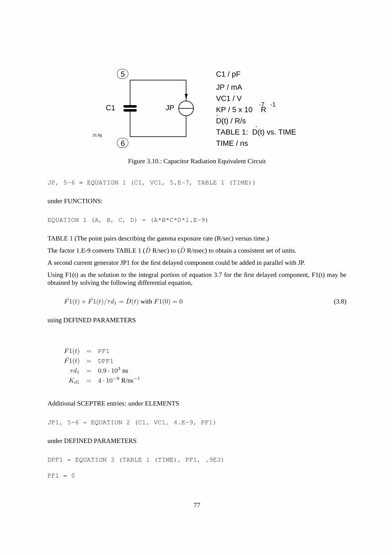
21.fig
6
5
C1 JP
JP / mA
TIME / ns
TABLE 1: D(t) vs. TIME
D(t) / R/s.
VC1 / V
C1 / pF
.
-7KP / 5 x 10 R
-1
Figure 3.10.: Capacitor Radiation Equivalent Circuit
JP, 5-6 = EQUATION 1 (C1, VC1, 5.E-7, TABLE 1 (TIME))
under FUNCTIONS:
EQUATION 1 (A, B, C, D) = (A*B*C*D*1.E-9)
TABLE 1 (The point pairs describing the gamma exposure rate (R/sec) versus time.)
The factor 1.E-9 converts TABLE 1 (D R/sec) to (D R/nsec) to obtain a consistent set of units.
A second current generator JP1 for the first delayed component could be added in parallel with JP.
Using F1(t) as the solution to the integral portion of equation 3.7 for the first delayed component, F1(t) may beobtained by solving the following differential equation,
F1(t) + F1(t)/τd1 = D(t) with F1(0) = 0 (3.8)
using DEFINED PARAMETERS
F1(t) = PF1
F1(t) = DPF1
τd1 = 0.9 · 103 ns
Kd1 = 4 · 10−9 R/ns−1
Additional SCEPTRE entries: under ELEMENTS
JP1, 5-6 = EQUATION 2 (C1, VC1, 4.E-9, PF1)
under DEFINED PARAMETERS
DPF1 = EQUATION 3 (TABLE 1 (TIME), PF1, .9E3)
PF1 = 0
77

under FUNCTIONS
EQUATION 2 (A, B, C, D) = (A*B*C*D)
EQUATION 3 (A, B, C) = (A*1.E-9-B/C)
The factor 1.E-9 converts TABLE 1 to nanosecond time units as in EQUATION 1.
78
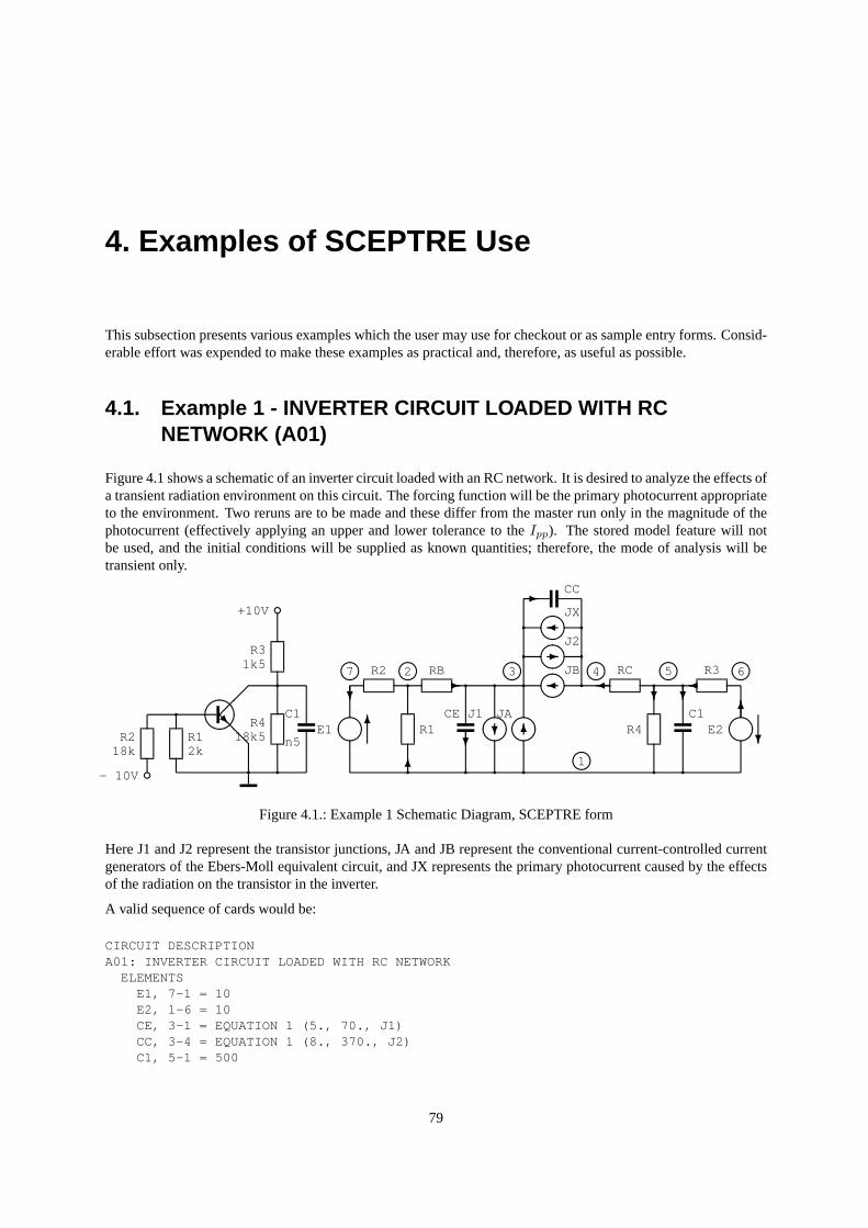
4. Examples of SCEPTRE Use
This subsection presents various examples which the user may use for checkout or as sample entry forms. Consid-erable effort was expended to make these examples as practical and, therefore, as useful as possible.
4.1. Example 1 - INVERTER CIRCUIT LOADED WITH RCNETWORK (A01)
Figure 4.1 shows a schematic of an inverter circuit loaded with an RC network. It is desired to analyze the effects ofa transient radiation environment on this circuit. The forcing function will be the primary photocurrent appropriateto the environment. Two reruns are to be made and these differ from the master run only in the magnitude of thephotocurrent (effectively applying an upper and lower tolerance to theIpp). The stored model feature will notbe used, and the initial conditions will be supplied as known quantities; therefore, the mode of analysis will betransient only.
c
c
qqq q
qq qqq q q
qqqqqq
q q q q? 6
-
6
?
6
?
-
-
? ?
6
?k
kkkk kk 654327
1
E1
R2 RB
R1J1 JA
CC
JX
J2
JB RC
R4
R3
E2R2
18kR12k
- 10V
+10V
R31k5
R418k5
C1
n5
R@@
C1CE
Figure 4.1.: Example 1 Schematic Diagram, SCEPTRE form
Here J1 and J2 represent the transistor junctions, JA and JB represent the conventional current-controlled currentgenerators of the Ebers-Moll equivalent circuit, and JX represents the primary photocurrent caused by the effectsof the radiation on the transistor in the inverter.
A valid sequence of cards would be:
CIRCUIT DESCRIPTIONA01: INVERTER CIRCUIT LOADED WITH RC NETWORK
ELEMENTSE1, 7-1 = 10E2, 1-6 = 10CE, 3-1 = EQUATION 1 (5., 70., J1)CC, 3-4 = EQUATION 1 (8., 370., J2)C1, 5-1 = 500
79
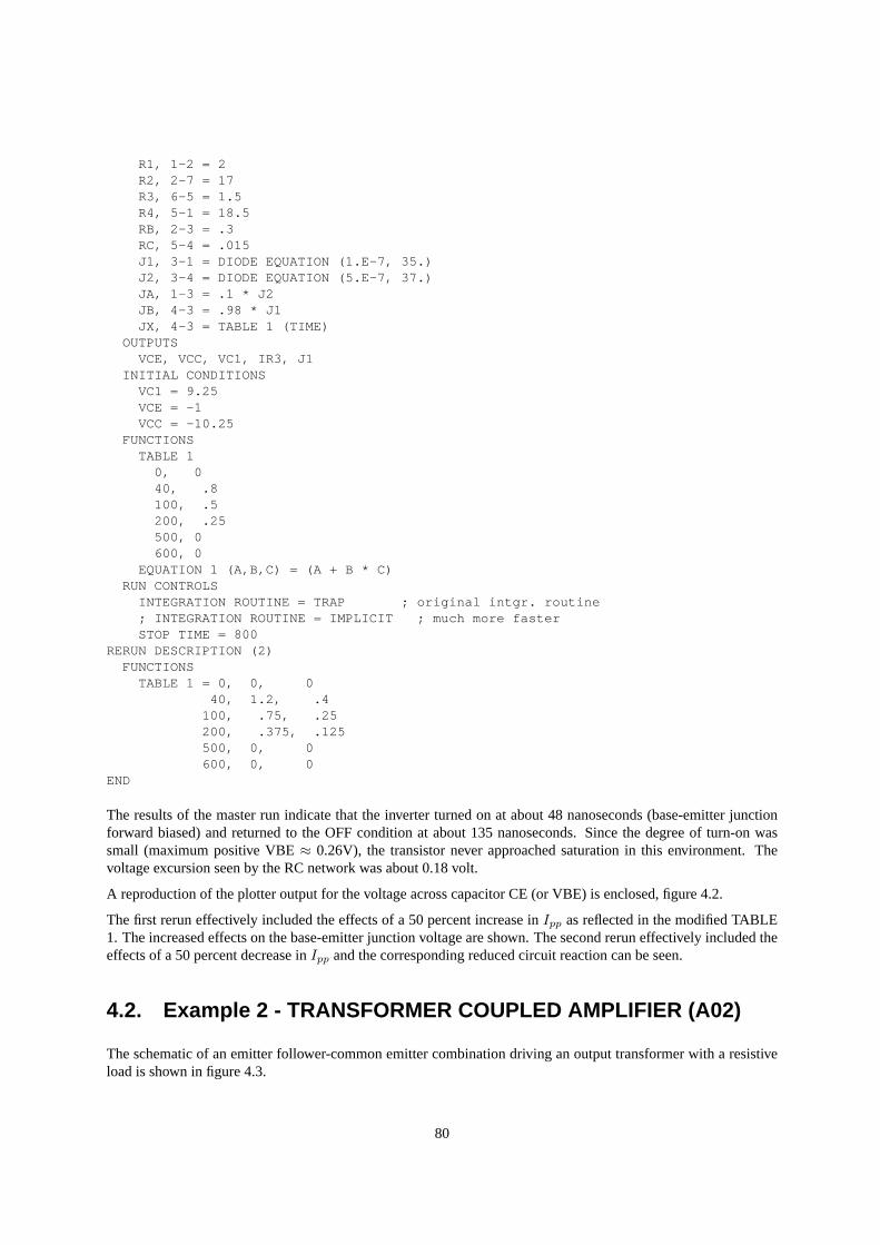
R1, 1-2 = 2R2, 2-7 = 17R3, 6-5 = 1.5R4, 5-1 = 18.5RB, 2-3 = .3RC, 5-4 = .015J1, 3-1 = DIODE EQUATION (1.E-7, 35.)J2, 3-4 = DIODE EQUATION (5.E-7, 37.)JA, 1-3 = .1 * J2JB, 4-3 = .98 * J1JX, 4-3 = TABLE 1 (TIME)
OUTPUTSVCE, VCC, VC1, IR3, J1
INITIAL CONDITIONSVC1 = 9.25VCE = -1VCC = -10.25
FUNCTIONSTABLE 1
0, 040, .8100, .5200, .25500, 0600, 0
EQUATION 1 (A,B,C) = (A + B * C)RUN CONTROLS
INTEGRATION ROUTINE = TRAP ; original intgr. routine; INTEGRATION ROUTINE = IMPLICIT ; much more fasterSTOP TIME = 800
RERUN DESCRIPTION (2)FUNCTIONS
TABLE 1 = 0, 0, 040, 1.2, .4
100, .75, .25200, .375, .125500, 0, 0600, 0, 0
END
The results of the master run indicate that the inverter turned on at about 48 nanoseconds (base-emitter junctionforward biased) and returned to the OFF condition at about 135 nanoseconds. Since the degree of turn-on wassmall (maximum positive VBE≈ 0.26V), the transistor never approached saturation in this environment. Thevoltage excursion seen by the RC network was about 0.18 volt.
A reproduction of the plotter output for the voltage across capacitor CE (or VBE) is enclosed, figure 4.2.
The first rerun effectively included the effects of a 50 percent increase inIpp as reflected in the modified TABLE1. The increased effects on the base-emitter junction voltage are shown. The second rerun effectively included theeffects of a 50 percent decrease inIpp and the corresponding reduced circuit reaction can be seen.
4.2. Example 2 - TRANSFORMER COUPLED AMPLIFIER (A02)
The schematic of an emitter follower-common emitter combination driving an output transformer with a resistiveload is shown in figure 4.3.
80
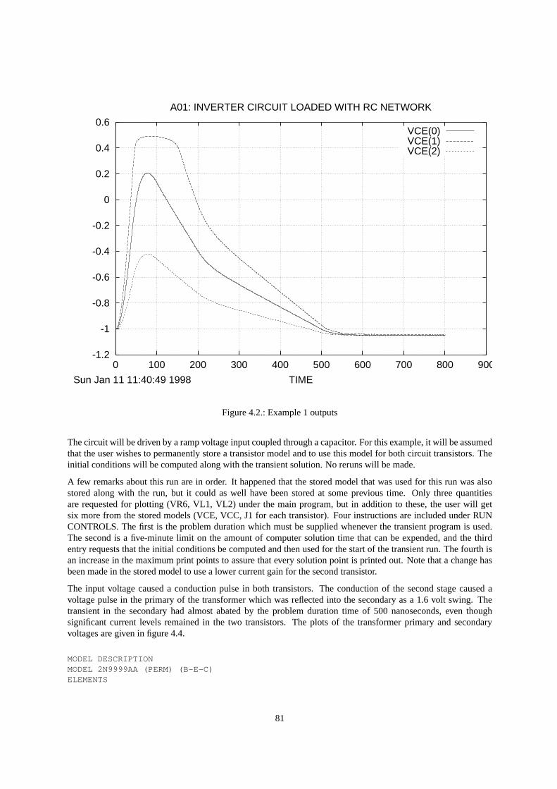
-1.2
-1
-0.8
-0.6
-0.4
-0.2
0
0.2
0.4
0.6
0 100 200 300 400 500 600 700 800 900
TIME
A01: INVERTER CIRCUIT LOADED WITH RC NETWORK
Sun Jan 11 11:40:49 1998
VCE(0)VCE(1)VCE(2)
Figure 4.2.: Example 1 outputs
The circuit will be driven by a ramp voltage input coupled through a capacitor. For this example, it will be assumedthat the user wishes to permanently store a transistor model and to use this model for both circuit transistors. Theinitial conditions will be computed along with the transient solution. No reruns will be made.
A few remarks about this run are in order. It happened that the stored model that was used for this run was alsostored along with the run, but it could as well have been stored at some previous time. Only three quantitiesare requested for plotting (VR6, VL1, VL2) under the main program, but in addition to these, the user will getsix more from the stored models (VCE, VCC, J1 for each transistor). Four instructions are included under RUNCONTROLS. The first is the problem duration which must be supplied whenever the transient program is used.The second is a five-minute limit on the amount of computer solution time that can be expended, and the thirdentry requests that the initial conditions be computed and then used for the start of the transient run. The fourth isan increase in the maximum print points to assure that every solution point is printed out. Note that a change hasbeen made in the stored model to use a lower current gain for the second transistor.
The input voltage caused a conduction pulse in both transistors. The conduction of the second stage caused avoltage pulse in the primary of the transformer which was reflected into the secondary as a 1.6 volt swing. Thetransient in the secondary had almost abated by the problem duration time of 500 nanoseconds, even thoughsignificant current levels remained in the two transistors. The plots of the transformer primary and secondaryvoltages are given in figure 4.4.
MODEL DESCRIPTIONMODEL 2N9999AA (PERM) (B-E-C)ELEMENTS
81
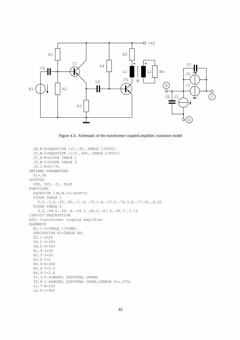
@@@
@@R
R
errr
r
r r
r r
r r
?E1
CZ
R1
T1
R2
R3
CX
R4
R5
L1
T1 M
L2 R6
+E2
e
e
e-
?
rr
r
r rr
B
E
C
CC
J2
J3
CE J1
Figure 4.3.: Schematic of the transformer coupled amplifier, transistor model
CE,B-E=EQUATION 1(5.,40.,TABLE 1(VCE))CC,B-C=EQUATION 1(10.,400.,TABLE 2(VCC))J1,B-E=DIODE TABLE 1J2,B-C=DIODE TABLE 2J3,C-B=P1*J1
DEFINED PARAMETERSP1=.98
OUTPUTSVCE, VCC, J1, PLOT
FUNCTIONSEQUATION 1(A,B,C)=(A+B*C)DIODE TABLE 1
0,0,.3,0,.65,.05,.7,.6,.72,1.4,.73,2,.74,3.4,.77,10,.8,22DIODE TABLE 2
0,0,.58,0,.62,.4,.64,1,.66,2,.67,3,.69,7,.7,12CIRCUIT DESCRIPTIONA02: transformer coupled amplifierELEMENTS
E1,1-2=TABLE 1(TIME)DERIVATIVE E1=TABLE DE1E2,1-4=20CZ,2-3=1E3CX,5-6=1E3R1,4-3=30R2,3-1=20R3,5-1=2R4,4-6=240R5,4-7=3.3R6,9-1=1.8T1,3-5-4=MODEL 2N9999AA (PERM)T2,6-1-8=MODEL 2N9999AA (PERM,CHANGE P1=.975)L1,7-8=100L2,9-1=900
82
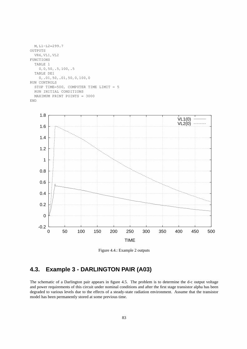
M,L1-L2=299.7OUTPUTS
VR6,VL1,VL2FUNCTIONS
TABLE 10,0,50,.5,100,.5
TABLE DE10,.01,50,.01,50,0,100,0
RUN CONTROLSSTOP TIME=500, COMPUTER TIME LIMIT = 5RUN INITIAL CONDITIONSMAXIMUM PRINT POINTS = 3000
END
-0.2
0
0.2
0.4
0.6
0.8
1
1.2
1.4
1.6
1.8
0 50 100 150 200 250 300 350 400 450 500
TIME
VL1(0)VL2(0)
Figure 4.4.: Example 2 outputs
4.3. Example 3 - DARLINGTON PAIR (A03)
The schematic of a Darlington pair appears in figure 4.5. The problem is to determine the d-c output voltageand power requirements of this circuit under nominal conditions and after the first stage transistor alpha has beendegraded to various levels due to the effects of a steady-state radiation environment. Assume that the transistormodel has been permanently stored at some previous time.
83
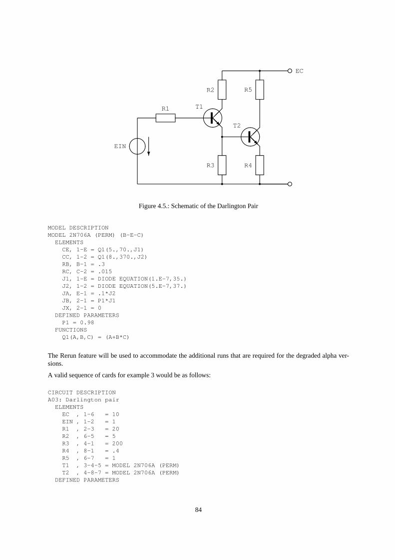
@@R
@@R
@@
@@
e
e
?EIN
R1
R2 R5
EC
T2
T1
R3 R4
r r
r
r
Figure 4.5.: Schematic of the Darlington Pair
MODEL DESCRIPTIONMODEL 2N706A (PERM) (B-E-C)
ELEMENTSCE, 1-E = Q1(5.,70.,J1)CC, 1-2 = Q1(8.,370.,J2)RB, B-1 = .3RC, C-2 = .015J1, 1-E = DIODE EQUATION(1.E-7,35.)J2, 1-2 = DIODE EQUATION(5.E-7,37.)JA, E-1 = .1*J2JB, 2-1 = P1*J1JX, 2-1 = 0
DEFINED PARAMETERSP1 = 0.98
FUNCTIONSQ1(A,B,C) = (A+B*C)
The Rerun feature will be used to accommodate the additional runs that are required for the degraded alpha ver-sions.
A valid sequence of cards for example 3 would be as follows:
CIRCUIT DESCRIPTIONA03: Darlington pair
ELEMENTSEC , 1-6 = 10EIN , 1-2 = 1R1 , 2-3 = 20R2 , 6-5 = 5R3 , 4-1 = 200R4 , 8-1 = .4R5 , 6-7 = 1T1 , 3-4-5 = MODEL 2N706A (PERM)T2 , 4-8-7 = MODEL 2N706A (PERM)
DEFINED PARAMETERS
84

I/C TRANSIENT VALUES AT TIME EQUALS ZERO:VCET1 = 3.3818865E-01VCCT1 =-8.9376695E+00VCET2 = 4.4221916E-01VCCT2 =-8.8226781E+00
RESULTS OF INITIAL CONDITION COMPUTATIONSPEC 5.3007344E+00PEIN 2.7598821E-04VR3 6.5620879E-01VR4 2.1082735E-01
I/C TRANSIENT VALUES AT TIME EQUALS ZERO:VCET1 = 3.3769191E-01VCCT1 =-8.9456210E+00VCET2 = 4.4163421E-01VCCT2 =-8.8381601E+00
RESULTS OF INITIAL CONDITION COMPUTATIONSRERUN 1
PEC 5.1910074E+00PEIN 5.4289718E-04VR3 6.5128728E-01VR4 2.0655488E-01
I/C TRANSIENT VALUES AT TIME EQUALS ZERO:VCET1 = 3.3696571E-01VCCT1 =-8.9570427E+00VCET2 = 4.4077602E-01VCCT2 =-8.8603292E+00
RESULTS OF INITIAL CONDITION COMPUTATIONSRERUN 2
PEC 5.0340188E+00PEIN 9.2654405E-04VR3 6.4422545E-01VR4 2.0044292E-01
I/C TRANSIENT VALUES AT TIME EQUALS ZERO:VCET1 = 3.3626101E-01VCCT1 =-8.9679012E+00VCET2 = 4.3993970E-01VCCT2 =-8.8813264E+00
RESULTS OF INITIAL CONDITION COMPUTATIONSRERUN 3
PEC 4.8854795E+00PEIN 1.2915639E-03VR3 6.3752024E-01VR4 1.9466077E-01
SIMULATION PROGRAM HAS TERMINATED
Figure 4.6.: Example 3 Output Listings
PEC = X1 (EC*IEC)PEIN= X2 (EIN*IEIN)
OUTPUTSPEC,PEIN,VR3,VR4
RUN CONTROLSRUN INITIAL CONDITIONS ONLY
RERUN DESCRIPTION (3)DEFINED PARAMETERS
P1T1= .96, .93, .9END
The RUN INITIAL CONDITIONS ONLY entry ensures that no transient computations will be made. The Newton-Raphson process will iterate to the final DC solution for the master run; then do the same for each of the reruns inturn.
Figure 4.6 shows the results of the master run and the three reruns in tabular form. There is little change betweenthe results of the master run and the reruns because of the inherent stability of the circuit. The power supplied fromthe input source EIN increases successively in the reruns because the reduced alpha of the first stage permits moreinput current.
85
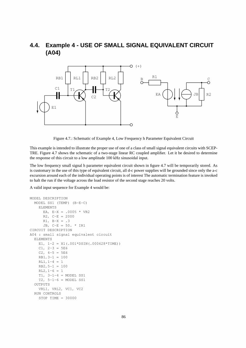
4.4. Example 4 - USE OF SMALL SIGNAL EQUIVALENT CIRCUIT(A04)
@@R @@R
@@
@@
?
e
e
ee
eE1
C1
RB1 RL1 RB2 RL2
C2
T1 T2
(+)
R1
EA JB??
R2
CB
E
r
r r r
r r
r rr r
r
Figure 4.7.: Schematic of Example 4, Low Frequency h Parameter Equivalent Circuit
This example is intended to illustrate the proper use of one of a class of small signal equivalent circuits with SCEP-TRE. Figure 4.7 shows the schematic of a two-stage linear RC coupled amplifier. Let it be desired to determinethe response of this circuit to a low amplitude 100 kHz sinusoidal input.
The low frequency small signal h parameter equivalent circuit shown in figure 4.7 will be temporarily stored. Asis customary in the use of this type of equivalent circuit, all d-c power supplies will be grounded since only the a-cexcursion around each of the individual operating points is of interest The automatic termination feature is invokedto halt the run if the voltage across the load resistor of the second stage reaches 20 volts.
A valid input sequence for Example 4 would be:
MODEL DESCRIPTIONMODEL SS1 (TEMP) (B-E-C)
ELEMENTSEA, E-X = .0005 * VR2R2, C-E = 2000R1, B-X = .3JB, C-E = 50. * IR1
CIRCUIT DESCRIPTIONA04 : small signal equivalent circuit
ELEMENTSE1, 1-2 = X1(.001*DSIN(.000628*TIME))C1, 2-3 = 5E6C2, 4-5 = 5E6RB1,3-1 = 100RL1,1-4 = 1RB2,5-1 = 100RL2,1-6 = 1T1, 3-1-4 = MODEL SS1T2, 5-1-6 = MODEL SS1
OUTPUTSVRL1, VRL2, VC1, VC2
RUN CONTROLSSTOP TIME = 30000
86
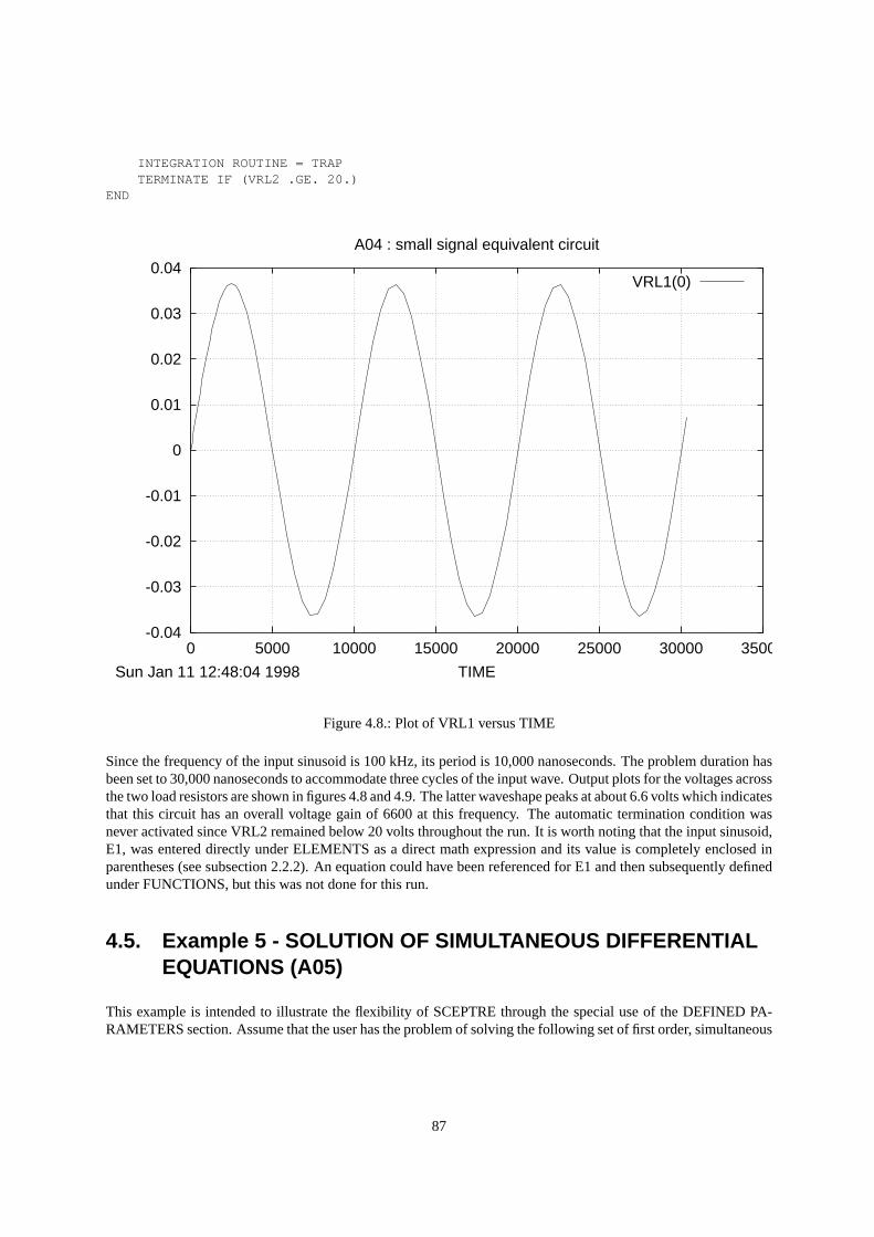
INTEGRATION ROUTINE = TRAPTERMINATE IF (VRL2 .GE. 20.)
END
-0.04
-0.03
-0.02
-0.01
0
0.01
0.02
0.03
0.04
0 5000 10000 15000 20000 25000 30000 35000
TIME
A04 : small signal equivalent circuit
Sun Jan 11 12:48:04 1998
VRL1(0)
Figure 4.8.: Plot of VRL1 versus TIME
Since the frequency of the input sinusoid is 100 kHz, its period is 10,000 nanoseconds. The problem duration hasbeen set to 30,000 nanoseconds to accommodate three cycles of the input wave. Output plots for the voltages acrossthe two load resistors are shown in figures 4.8 and 4.9. The latter waveshape peaks at about 6.6 volts which indicatesthat this circuit has an overall voltage gain of 6600 at this frequency. The automatic termination condition wasnever activated since VRL2 remained below 20 volts throughout the run. It is worth noting that the input sinusoid,E1, was entered directly under ELEMENTS as a direct math expression and its value is completely enclosed inparentheses (see subsection 2.2.2). An equation could have been referenced for E1 and then subsequently definedunder FUNCTIONS, but this was not done for this run.
4.5. Example 5 - SOLUTION OF SIMULTANEOUS DIFFERENTIALEQUATIONS (A05)
This example is intended to illustrate the flexibility of SCEPTRE through the special use of the DEFINED PA-RAMETERS section. Assume that the user has the problem of solving the following set of first order, simultaneous
87
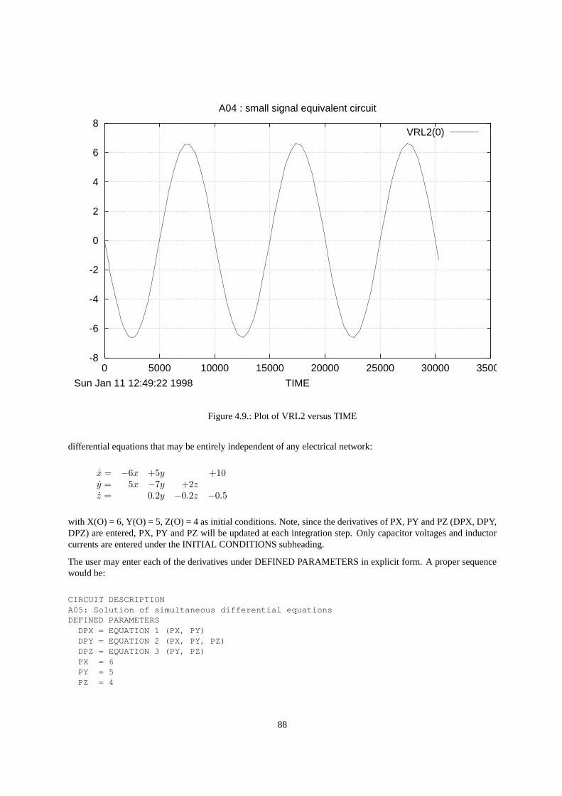
-8
-6
-4
-2
0
2
4
6
8
0 5000 10000 15000 20000 25000 30000 35000
TIME
A04 : small signal equivalent circuit
Sun Jan 11 12:49:22 1998
VRL2(0)
Figure 4.9.: Plot of VRL2 versus TIME
differential equations that may be entirely independent of any electrical network:
x = −6x +5y +10y = 5x −7y +2zz = 0.2y −0.2z −0.5
with X(O) = 6, Y(O) = 5, Z(O) = 4 as initial conditions. Note, since the derivatives of PX, PY and PZ (DPX, DPY,DPZ) are entered, PX, PY and PZ will be updated at each integration step. Only capacitor voltages and inductorcurrents are entered under the INITIAL CONDITIONS subheading.
The user may enter each of the derivatives under DEFINED PARAMETERS in explicit form. A proper sequencewould be:
CIRCUIT DESCRIPTIONA05: Solution of simultaneous differential equationsDEFINED PARAMETERS
DPX = EQUATION 1 (PX, PY)DPY = EQUATION 2 (PX, PY, PZ)DPZ = EQUATION 3 (PY, PZ)PX = 6PY = 5PZ = 4
88
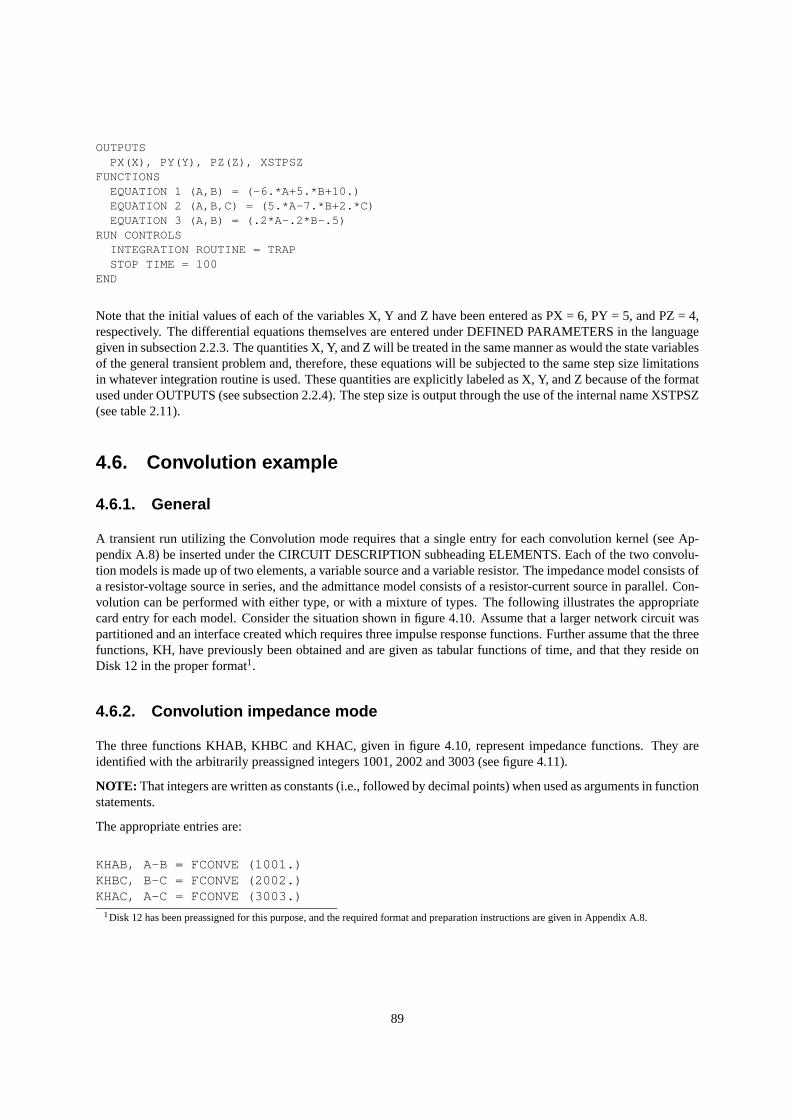
OUTPUTSPX(X), PY(Y), PZ(Z), XSTPSZ
FUNCTIONSEQUATION 1 (A,B) = (-6.*A+5.*B+10.)EQUATION 2 (A,B,C) = (5.*A-7.*B+2.*C)EQUATION 3 (A,B) = (.2*A-.2*B-.5)
RUN CONTROLSINTEGRATION ROUTINE = TRAPSTOP TIME = 100
END
Note that the initial values of each of the variables X, Y and Z have been entered as PX = 6, PY = 5, and PZ = 4,respectively. The differential equations themselves are entered under DEFINED PARAMETERS in the languagegiven in subsection 2.2.3. The quantities X, Y, and Z will be treated in the same manner as would the state variablesof the general transient problem and, therefore, these equations will be subjected to the same step size limitationsin whatever integration routine is used. These quantities are explicitly labeled as X, Y, and Z because of the formatused under OUTPUTS (see subsection 2.2.4). The step size is output through the use of the internal name XSTPSZ(see table 2.11).
4.6. Convolution example
4.6.1. General
A transient run utilizing the Convolution mode requires that a single entry for each convolution kernel (see Ap-pendix A.8) be inserted under the CIRCUIT DESCRIPTION subheading ELEMENTS. Each of the two convolu-tion models is made up of two elements, a variable source and a variable resistor. The impedance model consists ofa resistor-voltage source in series, and the admittance model consists of a resistor-current source in parallel. Con-volution can be performed with either type, or with a mixture of types. The following illustrates the appropriatecard entry for each model. Consider the situation shown in figure 4.10. Assume that a larger network circuit waspartitioned and an interface created which requires three impulse response functions. Further assume that the threefunctions, KH, have previously been obtained and are given as tabular functions of time, and that they reside onDisk 12 in the proper format1.
4.6.2. Convolution impedance mode
The three functions KHAB, KHBC and KHAC, given in figure 4.10, represent impedance functions. They areidentified with the arbitrarily preassigned integers 1001, 2002 and 3003 (see figure 4.11).
NOTE: That integers are written as constants (i.e., followed by decimal points) when used as arguments in functionstatements.
The appropriate entries are:
KHAB, A-B = FCONVE (1001.)KHBC, B-C = FCONVE (2002.)KHAC, A-C = FCONVE (3003.)
1Disk 12 has been preassigned for this purpose, and the required format and preparation instructions are given in Appendix A.8.
89
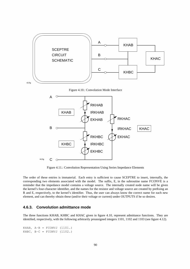
A
B
C
SCEPTRE
CIRCUIT
SCHEMATIC
43.fig
KHBC
KHAB
KHAC
Figure 4.10.: Convolution Mode Interface
44.fig
A
B
C
KHAC
KHBC
KHAB
RKHAB
EKHAB RKHAC
EKHACRKHBC
EKHBC
IRKHAC
IRKHBC
IRKHAB
Figure 4.11.: Convolution Representation Using Series Impedance Elements
The order of these entries is immaterial. Each entry is sufficient to cause SCEPTRE to insert, internally, thecorresponding two elements associated with the model. The suffix, E, in the subroutine name FCONVE is areminder that the impedance model contains a voltage source. The internally created node name will be giventhe kernel’s four-character identifier, and the names for the resistor and voltage source are created by prefixing anR and E, respectively, to the kernel’s identifier. Thus, the user can always know the correct name for each newelement, and can thereby obtain these (and/or their voltage or current) under OUTPUTS if he so desires.
4.6.3. Convolution admittance mode
The three functions KHAB, KHBC and KHAC given in figure 4.10, represent admittance functions. They areidentified, respectively, with the following arbitrarily preassigned integers 1101, 1102 and 1103 (see figure 4.12).
KHAB, A-B = FCONVJ (1101.)KHBC, B-C = FCONVJ (1102.)
90
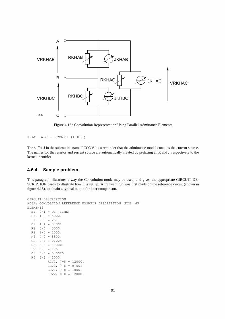
A
B
C
RKHBC
RKHAB JKHAB
JKHBC
RKHAC JKHAC VRKHAC
VRKHAB
VRKHBC
45.fig
Figure 4.12.: Convolution Representation Using Parallel Admittance Elements
KHAC, A-C - FCONVJ (1103.)
The suffix J in the subroutine name FCONVJ is a reminder that the admittance model contains the current source.The names for the resistor and surrent source are automatically created by prefixing an R and J, respectively to thekernel identifier.
4.6.4. Sample problem
This paragraph illustrates a way the Convolution mode may be used, and gives the appropriate CIRCUIT DE-SCRIPTION cards to illustrate how it is set up. A transient run was first made on the reference circuit (shown infigure 4.13), to obtain a typical output for later comparison.
CIRCUIT DESCRIPTIONA06A: CONVOLTION REFERENCE EXAMPLE DESCRIPTION (FIG. 47)ELEMENTS
E1, 0-1 = Q1 (TIME)R1, 1-2 = 5000.L1, 2-3 = 25.C1, 1-4 = 0.001R2, 3-4 = 3000.R3, 3-5 = 2000.R4, 4-0 = 8500.C2, 4-6 = 0.004R5, 5-6 = 11000.L2, 6-0 = 175.C3, 5-7 = 0.0025R6, 6-8 = 1000.
RCV1, 7-8 = 12000.CCV1, 7-8 = 0.001LCV1, 7-8 = 1000.RCV2, 8-0 = 12000.
91
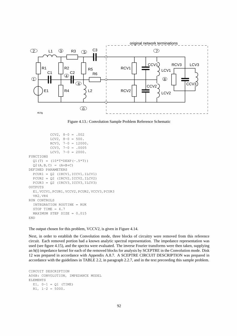
CCV1
CCV2
LCV1
LCV2
original network terminations
R5
1
5
0
8
R1C1
R2C2
R3
R6
C3L1
R4 L2E1
3
4
6
2 7
RCV1
RCV2
LCV3RCV3
CCV3
46.fig
Figure 4.13.: Convolution Sample Problem Reference Schematic
CCV2, 8-0 = .002LCV2, 8-0 = 500.RCV3, 7-0 = 12000.CCV3, 7-0 = .0005LCV3, 7-0 = 2000.
FUNCTIONSQ1(T) = (10*T*DEXP(-.5*T))Q2(A,B,C) = (A+B+C)
DEFINED PARAMETERSPCUR1 = Q2 (IRCV1,ICCV1,ILCV1)PCUR2 = Q2 (IRCV2,ICCV2,ILCV2)PCUR3 = Q2 (IRCV3,ICCV3,ILCV3)
OUTPUTSE1,VCCV1,PCUR1,VCCV2,PCUR2,VCCV3,PCUR3VR2,VR4
RUN CONTROLSINTEGRATION ROUTINE = RUKSTOP TIME = 4.7MAXIMUM STEP SIZE = 0.015
END
The output chosen for this problem, VCCV2, is given in Figure 4.14.
Next, in order to establish the Convolution mode, three blocks of circuitry were removed from this referencecircuit. Each removed portion had a known analytic spectral representation. The impedance representation wasused (see figure 4.15), and the spectra were evaluated. The inverse Fourier transforms were then taken, supplyingan h(t) impedance kernel for each of the removed blocks for analysis by SCEPTRE in the Convolution mode. Disk12 was prepared in accordance with Appendix A.8.7. A SCEPTRE CIRCUIT DESCRIPTION was prepared inaccordance with the guidelines in TABLE 2.2, in paragraph 2.2.7, and in the text preceeding this sample problem.
CIRCUIT DESCRIPTIONA06B: CONVOLUTION, IMPEDANCE MODELELEMENTS
E1, 0-1 = Ql (TIME)R1, 1-2 = 5000.
92
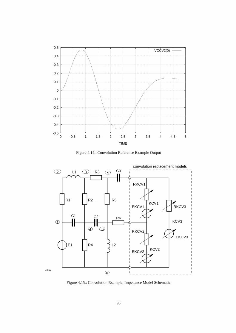
-0.5
-0.4
-0.3
-0.2
-0.1
0
0.1
0.2
0.3
0.4
0.5
0 0.5 1 1.5 2 2.5 3 3.5 4 4.5 5
TIME
VCCV2(0)
Figure 4.14.: Convolution Reference Example Output
5R3 C3L12
R4 L2E1
1
C1 C2
R2R1
R6
R5
64
0
3
49.fig
RKCV3
EKCV3
KCV1
KCV2
KCV3
convolution replacement models
RKCV1
EKCV1
RKCV2
EKCV2
Figure 4.15.: Convolution Example, Impedance Model Schematic
93

Plot not available!Figure 4.16.: Convolution Sample Problem Output
L1, 2-3 = 25.C1, 1-4 = .001R2, 3-4 = 3000.R3, 3-5 = 2000.R4, 4-0 = 8500.C2, 4-6 = .004R5, 5-6 = 11000.L2, 6-0 = 175C3, 5-7 = .0025R6, 6-8 = 1000.
KCV1, 7-8 = FCONVE(1001.)KCV2, 8-0 = FCONVE(1002.)KCV3, 7-0 = FCONVE(1003.)
FUNCTIONSQl(T) = (10*T*DEXP(-.5*T)Q2(A,B) = (A+B)
DEFINED PARAMETERSPVOLT1 = Q2(VRKCV1, EKCV1)PVOLT2 = Q2 (VRKCV2, EKCV2)PVOLT3 = Q2(VRKCV3, EKCV3)
OUTPUTSE1, PLOTIRKCV1, IRKCV2, IRKCV3, PLOTPVOLT1, PVOLT2, PVOLT3, PLOTVR2, VR4
RUN CONTROLSINTEGRATION ROUTINE=RUKWRITE SIMUL8 DATAPRINT B MATRIXSTOP TIME = 4.7MAXIMUM STEP SIZE = 0.15IMPULSE RESPONSE BUFFER = 300INPUT FUNCTION BUFFER = 900
END
Figure 4.16 shows the output voltage across the same nodes as were used for the reference circuit, figure 4.13.
4.7. Example 7 - USE OF MONTE CARLO (A07)
The Darlington Pair used for Example 3 and shown in figure 4.5 is used also to demonstrate the Monte Carlo option.While all four of the DC options (Monte Carlo, Sensitivity, Worst-Case and Optimization) can be requested in asingle run, they are shown separately in this and the next three examples for clarity. In each case, the completeSCEPTRE input deck is listed, and the output due to execution of the requested feature is shown.
MODEL DESCRIPTIONMODEL 2N706A (TEMP) (B-E-C)
94
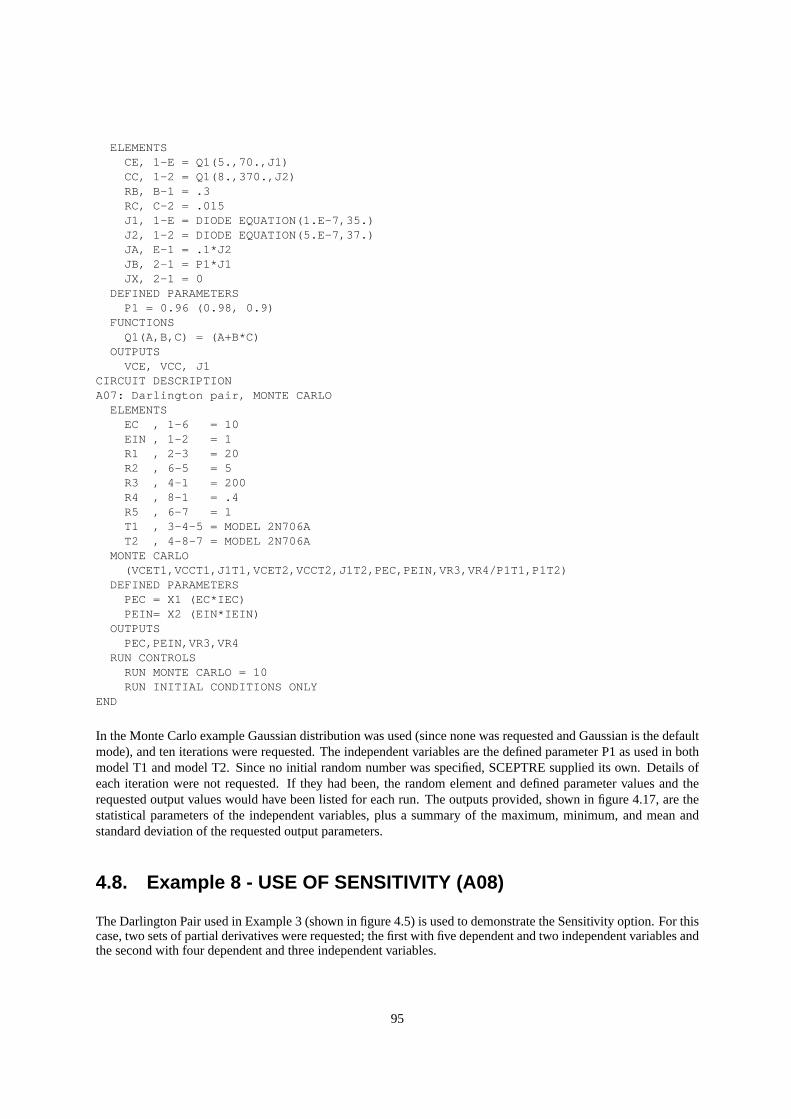
ELEMENTSCE, 1-E = Q1(5.,70.,J1)CC, 1-2 = Q1(8.,370.,J2)RB, B-1 = .3RC, C-2 = .015J1, 1-E = DIODE EQUATION(1.E-7,35.)J2, 1-2 = DIODE EQUATION(5.E-7,37.)JA, E-1 = .1*J2JB, 2-1 = P1*J1JX, 2-1 = 0
DEFINED PARAMETERSP1 = 0.96 (0.98, 0.9)
FUNCTIONSQ1(A,B,C) = (A+B*C)
OUTPUTSVCE, VCC, J1
CIRCUIT DESCRIPTIONA07: Darlington pair, MONTE CARLO
ELEMENTSEC , 1-6 = 10EIN , 1-2 = 1R1 , 2-3 = 20R2 , 6-5 = 5R3 , 4-1 = 200R4 , 8-1 = .4R5 , 6-7 = 1T1 , 3-4-5 = MODEL 2N706AT2 , 4-8-7 = MODEL 2N706A
MONTE CARLO(VCET1,VCCT1,J1T1,VCET2,VCCT2,J1T2,PEC,PEIN,VR3,VR4/P1T1,P1T2)
DEFINED PARAMETERSPEC = X1 (EC*IEC)PEIN= X2 (EIN*IEIN)
OUTPUTSPEC,PEIN,VR3,VR4
RUN CONTROLSRUN MONTE CARLO = 10RUN INITIAL CONDITIONS ONLY
END
In the Monte Carlo example Gaussian distribution was used (since none was requested and Gaussian is the defaultmode), and ten iterations were requested. The independent variables are the defined parameter P1 as used in bothmodel T1 and model T2. Since no initial random number was specified, SCEPTRE supplied its own. Details ofeach iteration were not requested. If they had been, the random element and defined parameter values and therequested output values would have been listed for each run. The outputs provided, shown in figure 4.17, are thestatistical parameters of the independent variables, plus a summary of the maximum, minimum, and mean andstandard deviation of the requested output parameters.
4.8. Example 8 - USE OF SENSITIVITY (A08)
The Darlington Pair used in Example 3 (shown in figure 4.5) is used to demonstrate the Sensitivity option. For thiscase, two sets of partial derivatives were requested; the first with five dependent and two independent variables andthe second with four dependent and three independent variables.
95
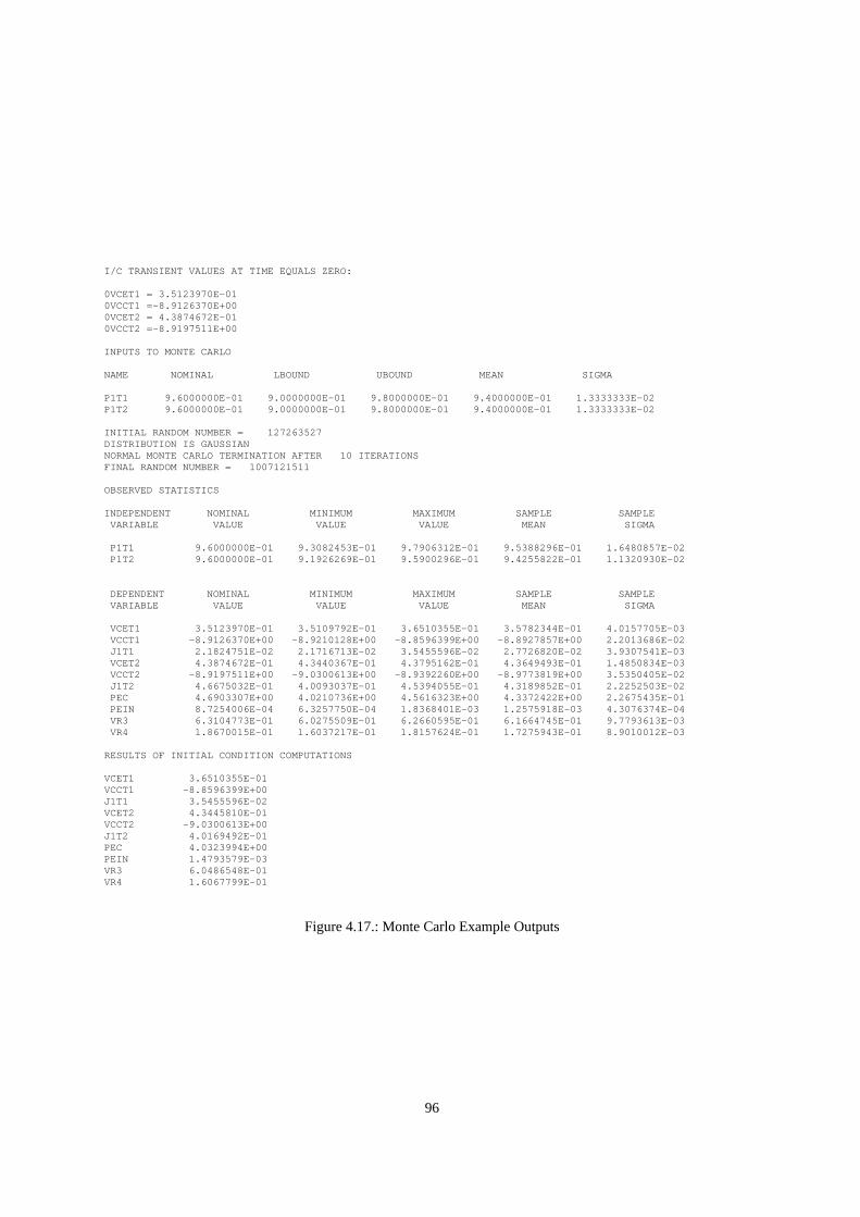
I/C TRANSIENT VALUES AT TIME EQUALS ZERO:
0VCET1 = 3.5123970E-010VCCT1 =-8.9126370E+000VCET2 = 4.3874672E-010VCCT2 =-8.9197511E+00
INPUTS TO MONTE CARLO
NAME NOMINAL LBOUND UBOUND MEAN SIGMA
P1T1 9.6000000E-01 9.0000000E-01 9.8000000E-01 9.4000000E-01 1.3333333E-02P1T2 9.6000000E-01 9.0000000E-01 9.8000000E-01 9.4000000E-01 1.3333333E-02
INITIAL RANDOM NUMBER = 127263527DISTRIBUTION IS GAUSSIANNORMAL MONTE CARLO TERMINATION AFTER 10 ITERATIONSFINAL RANDOM NUMBER = 1007121511
OBSERVED STATISTICS
INDEPENDENT NOMINAL MINIMUM MAXIMUM SAMPLE SAMPLEVARIABLE VALUE VALUE VALUE MEAN SIGMA
P1T1 9.6000000E-01 9.3082453E-01 9.7906312E-01 9.5388296E-01 1.6480857E-02P1T2 9.6000000E-01 9.1926269E-01 9.5900296E-01 9.4255822E-01 1.1320930E-02
DEPENDENT NOMINAL MINIMUM MAXIMUM SAMPLE SAMPLEVARIABLE VALUE VALUE VALUE MEAN SIGMA
VCET1 3.5123970E-01 3.5109792E-01 3.6510355E-01 3.5782344E-01 4.0157705E-03VCCT1 -8.9126370E+00 -8.9210128E+00 -8.8596399E+00 -8.8927857E+00 2.2013686E-02J1T1 2.1824751E-02 2.1716713E-02 3.5455596E-02 2.7726820E-02 3.9307541E-03VCET2 4.3874672E-01 4.3440367E-01 4.3795162E-01 4.3649493E-01 1.4850834E-03VCCT2 -8.9197511E+00 -9.0300613E+00 -8.9392260E+00 -8.9773819E+00 3.5350405E-02J1T2 4.6675032E-01 4.0093037E-01 4.5394055E-01 4.3189852E-01 2.2252503E-02PEC 4.6903307E+00 4.0210736E+00 4.5616323E+00 4.3372422E+00 2.2675435E-01PEIN 8.7254006E-04 6.3257750E-04 1.8368401E-03 1.2575918E-03 4.3076374E-04VR3 6.3104773E-01 6.0275509E-01 6.2660595E-01 6.1664745E-01 9.7793613E-03VR4 1.8670015E-01 1.6037217E-01 1.8157624E-01 1.7275943E-01 8.9010012E-03
RESULTS OF INITIAL CONDITION COMPUTATIONS
VCET1 3.6510355E-01VCCT1 -8.8596399E+00J1T1 3.5455596E-02VCET2 4.3445810E-01VCCT2 -9.0300613E+00J1T2 4.0169492E-01PEC 4.0323994E+00PEIN 1.4793579E-03VR3 6.0486548E-01VR4 1.6067799E-01
Figure 4.17.: Monte Carlo Example Outputs
96
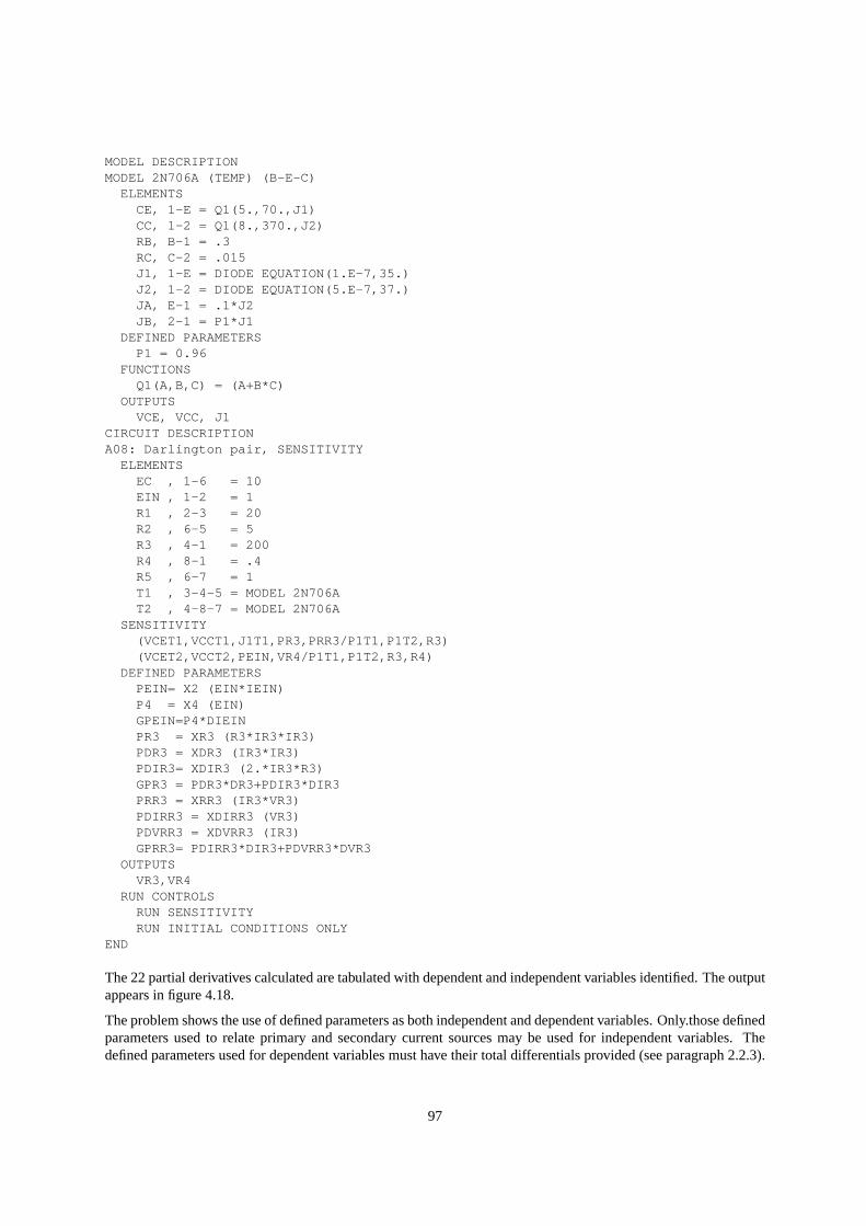
MODEL DESCRIPTIONMODEL 2N706A (TEMP) (B-E-C)
ELEMENTSCE, 1-E = Q1(5.,70.,J1)CC, 1-2 = Q1(8.,370.,J2)RB, B-1 = .3RC, C-2 = .015J1, 1-E = DIODE EQUATION(1.E-7,35.)J2, 1-2 = DIODE EQUATION(5.E-7,37.)JA, E-1 = .1*J2JB, 2-1 = P1*J1
DEFINED PARAMETERSP1 = 0.96
FUNCTIONSQ1(A,B,C) = (A+B*C)
OUTPUTSVCE, VCC, J1
CIRCUIT DESCRIPTIONA08: Darlington pair, SENSITIVITY
ELEMENTSEC , 1-6 = 10EIN , 1-2 = 1R1 , 2-3 = 20R2 , 6-5 = 5R3 , 4-1 = 200R4 , 8-1 = .4R5 , 6-7 = 1T1 , 3-4-5 = MODEL 2N706AT2 , 4-8-7 = MODEL 2N706A
SENSITIVITY(VCET1,VCCT1,J1T1,PR3,PRR3/P1T1,P1T2,R3)(VCET2,VCCT2,PEIN,VR4/P1T1,P1T2,R3,R4)
DEFINED PARAMETERSPEIN= X2 (EIN*IEIN)P4 = X4 (EIN)GPEIN=P4*DIEINPR3 = XR3 (R3*IR3*IR3)PDR3 = XDR3 (IR3*IR3)PDIR3= XDIR3 (2.*IR3*R3)GPR3 = PDR3*DR3+PDIR3*DIR3PRR3 = XRR3 (IR3*VR3)PDIRR3 = XDIRR3 (VR3)PDVRR3 = XDVRR3 (IR3)GPRR3= PDIRR3*DIR3+PDVRR3*DVR3
OUTPUTSVR3,VR4
RUN CONTROLSRUN SENSITIVITYRUN INITIAL CONDITIONS ONLY
END
The 22 partial derivatives calculated are tabulated with dependent and independent variables identified. The outputappears in figure 4.18.
The problem shows the use of defined parameters as both independent and dependent variables. Only.those definedparameters used to relate primary and secondary current sources may be used for independent variables. Thedefined parameters used for dependent variables must have their total differentials provided (see paragraph 2.2.3).
97
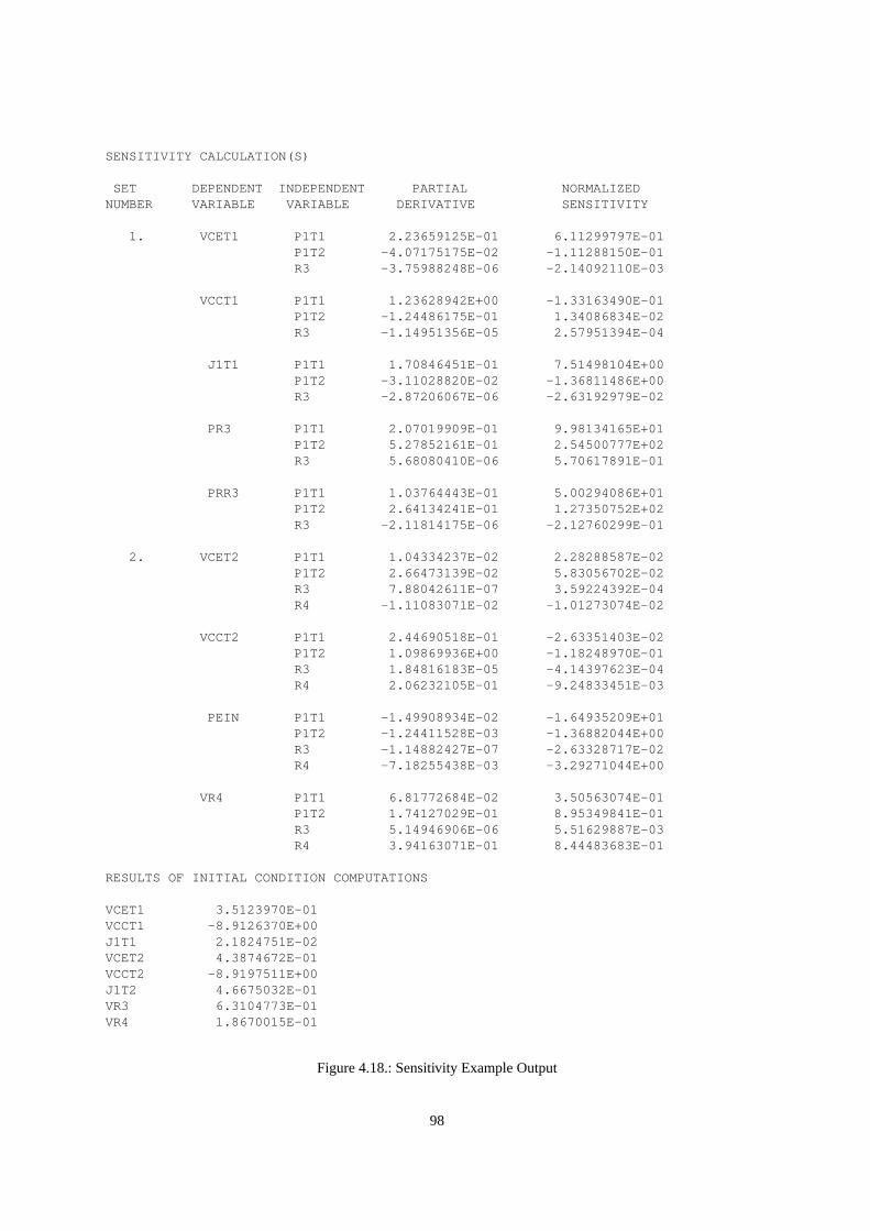
SENSITIVITY CALCULATION(S)
SET DEPENDENT INDEPENDENT PARTIAL NORMALIZEDNUMBER VARIABLE VARIABLE DERIVATIVE SENSITIVITY
1. VCET1 P1T1 2.23659125E-01 6.11299797E-01P1T2 -4.07175175E-02 -1.11288150E-01R3 -3.75988248E-06 -2.14092110E-03
VCCT1 P1T1 1.23628942E+00 -1.33163490E-01P1T2 -1.24486175E-01 1.34086834E-02R3 -1.14951356E-05 2.57951394E-04
J1T1 P1T1 1.70846451E-01 7.51498104E+00P1T2 -3.11028820E-02 -1.36811486E+00R3 -2.87206067E-06 -2.63192979E-02
PR3 P1T1 2.07019909E-01 9.98134165E+01P1T2 5.27852161E-01 2.54500777E+02R3 5.68080410E-06 5.70617891E-01
PRR3 P1T1 1.03764443E-01 5.00294086E+01P1T2 2.64134241E-01 1.27350752E+02R3 -2.11814175E-06 -2.12760299E-01
2. VCET2 P1T1 1.04334237E-02 2.28288587E-02P1T2 2.66473139E-02 5.83056702E-02R3 7.88042611E-07 3.59224392E-04R4 -1.11083071E-02 -1.01273074E-02
VCCT2 P1T1 2.44690518E-01 -2.63351403E-02P1T2 1.09869936E+00 -1.18248970E-01R3 1.84816183E-05 -4.14397623E-04R4 2.06232105E-01 -9.24833451E-03
PEIN P1T1 -1.49908934E-02 -1.64935209E+01P1T2 -1.24411528E-03 -1.36882044E+00R3 -1.14882427E-07 -2.63328717E-02R4 -7.18255438E-03 -3.29271044E+00
VR4 P1T1 6.81772684E-02 3.50563074E-01P1T2 1.74127029E-01 8.95349841E-01R3 5.14946906E-06 5.51629887E-03R4 3.94163071E-01 8.44483683E-01
RESULTS OF INITIAL CONDITION COMPUTATIONS
VCET1 3.5123970E-01VCCT1 -8.9126370E+00J1T1 2.1824751E-02VCET2 4.3874672E-01VCCT2 -8.9197511E+00J1T2 4.6675032E-01VR3 6.3104773E-01VR4 1.8670015E-01
Figure 4.18.: Sensitivity Example Output
98
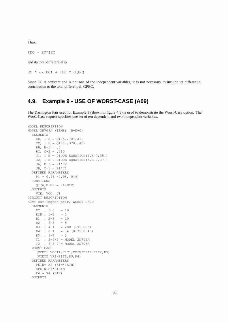
Thus,
PEC = EC*IEC
and its total differential is
EC * d(IEC) + IEC * d(EC)
Since EC is constant and is not one of the independent variables, it is not necessary to include its differentialcontribution to the total differential, GPEC.
4.9. Example 9 - USE OF WORST-CASE (A09)
The Darlington Pair used for Example 3 (shown in figure 4.5) is used to demonstrate the Worst-Case option. TheWorst-Case request specifies one set of ten dependent and two independent variables.
MODEL DESCRIPTIONMODEL 2N706A (TEMP) (B-E-C)
ELEMENTSCE, 1-E = Q1(5.,70.,J1)CC, 1-2 = Q1(8.,370.,J2)RB, B-1 = .3RC, C-2 = .015J1, 1-E = DIODE EQUATION(1.E-7,35.)J2, 1-2 = DIODE EQUATION(5.E-7,37.)JA, E-1 = .1*J2JB, 2-1 = P1*J1
DEFINED PARAMETERSP1 = 0.96 (0.98, 0.9)
FUNCTIONSQ1(A,B,C) = (A+B*C)
OUTPUTSVCE, VCC, J1
CIRCUIT DESCRIPTIONA09: Darlington pair, WORST CASE
ELEMENTSEC , 1-6 = 10EIN , 1-2 = 1R1 , 2-3 = 20R2 , 6-5 = 5R3 , 4-1 = 200 (195,205)R4 , 8-1 = .4 (0.35,0.45)R5 , 6-7 = 1T1 , 3-4-5 = MODEL 2N706AT2 , 4-8-7 = MODEL 2N706A
WORST CASE(VCET1,VCCT1,J1T1,PEIN/P1T1,P1T2,R3)(VCET2,VR4/P1T2,R3,R4)
DEFINED PARAMETERSPEIN= X2 (EIN*IEIN)GPEIN=P4*DIEINP4 = X4 (EIN)
OUTPUTS
99
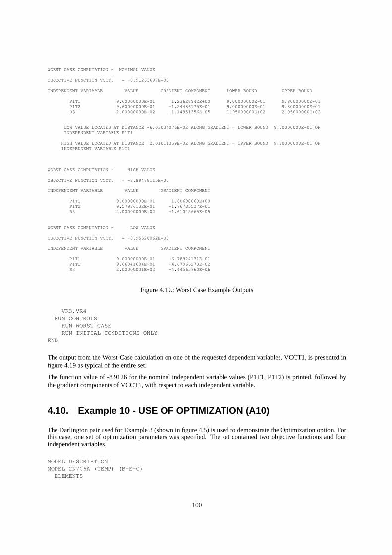
WORST CASE COMPUTATION - NOMINAL VALUE
OBJECTIVE FUNCTION VCCT1 = -8.91263697E+00
INDEPENDENT VARIABLE VALUE GRADIENT COMPONENT LOWER BOUND UPPER BOUND
P1T1 9.60000000E-01 1.23628942E+00 9.00000000E-01 9.80000000E-01P1T2 9.60000000E-01 -1.24486175E-01 9.00000000E-01 9.80000000E-01R3 2.00000000E+02 -1.14951356E-05 1.95000000E+02 2.05000000E+02
LOW VALUE LOCATED AT DISTANCE -6.03034076E-02 ALONG GRADIENT = LOWER BOUND 9.00000000E-01 OFINDEPENDENT VARIABLE P1T1
HIGH VALUE LOCATED AT DISTANCE 2.01011359E-02 ALONG GRADIENT = UPPER BOUND 9.80000000E-01 OFINDEPENDENT VARIABLE P1T1
WORST CASE COMPUTATION - HIGH VALUE
OBJECTIVE FUNCTION VCCT1 = -8.89478115E+00
INDEPENDENT VARIABLE VALUE GRADIENT COMPONENT
P1T1 9.80000000E-01 1.60698069E+00P1T2 9.57986132E-01 -1.76735527E-01R3 2.00000000E+02 -1.61045665E-05
WORST CASE COMPUTATION - LOW VALUE
OBJECTIVE FUNCTION VCCT1 = -8.95520062E+00
INDEPENDENT VARIABLE VALUE GRADIENT COMPONENT
P1T1 9.00000000E-01 6.78924171E-01P1T2 9.66041604E-01 -4.67066273E-02R3 2.00000001E+02 -4.44565760E-06
Figure 4.19.: Worst Case Example Outputs
VR3,VR4RUN CONTROLS
RUN WORST CASERUN INITIAL CONDITIONS ONLY
END
The output from the Worst-Case calculation on one of the requested dependent variables, VCCT1, is presented infigure 4.19 as typical of the entire set.
The function value of -8.9126 for the nominal independent variable values (P1T1, P1T2) is printed, followed bythe gradient components of VCCT1, with respect to each independent variable.
4.10. Example 10 - USE OF OPTIMIZATION (A10)
The Darlington pair used for Example 3 (shown in figure 4.5) is used to demonstrate the Optimization option. Forthis case, one set of optimization parameters was specified. The set contained two objective functions and fourindependent variables.
MODEL DESCRIPTIONMODEL 2N706A (TEMP) (B-E-C)
ELEMENTS
100
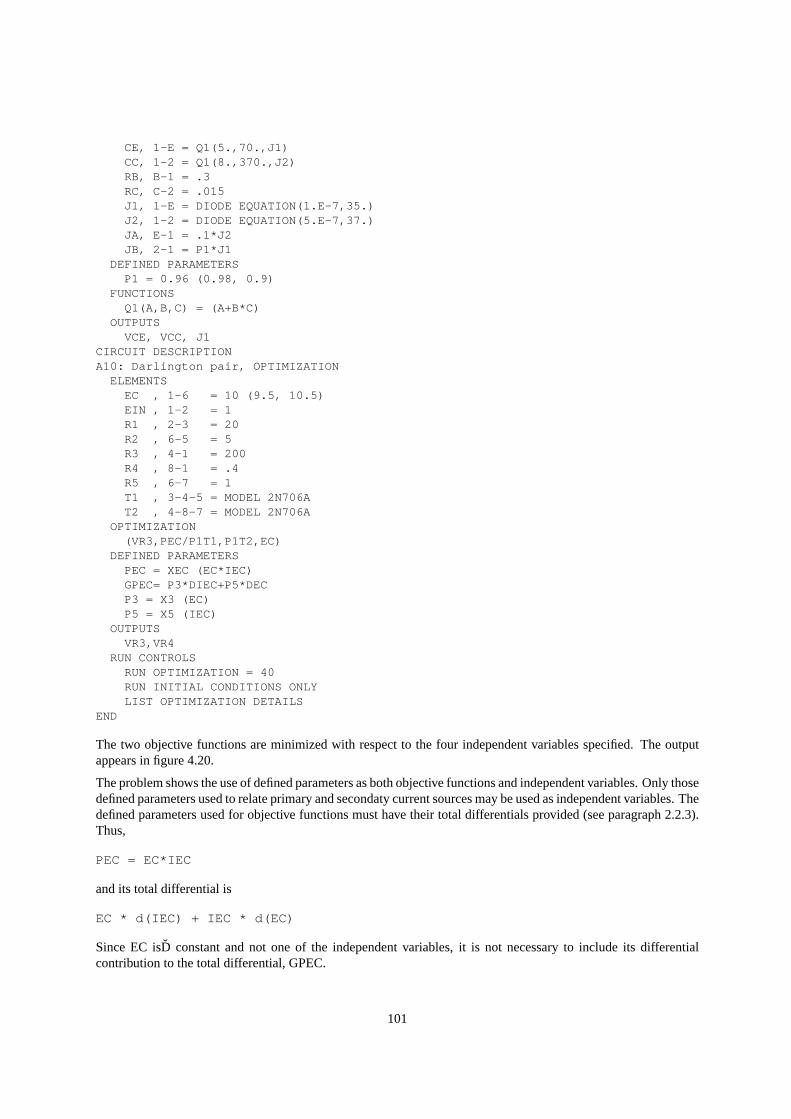
CE, 1-E = Q1(5.,70.,J1)CC, 1-2 = Q1(8.,370.,J2)RB, B-1 = .3RC, C-2 = .015J1, 1-E = DIODE EQUATION(1.E-7,35.)J2, 1-2 = DIODE EQUATION(5.E-7,37.)JA, E-1 = .1*J2JB, 2-1 = P1*J1
DEFINED PARAMETERSP1 = 0.96 (0.98, 0.9)
FUNCTIONSQ1(A,B,C) = (A+B*C)
OUTPUTSVCE, VCC, J1
CIRCUIT DESCRIPTIONA10: Darlington pair, OPTIMIZATION
ELEMENTSEC , 1-6 = 10 (9.5, 10.5)EIN , 1-2 = 1R1 , 2-3 = 20R2 , 6-5 = 5R3 , 4-1 = 200R4 , 8-1 = .4R5 , 6-7 = 1T1 , 3-4-5 = MODEL 2N706AT2 , 4-8-7 = MODEL 2N706A
OPTIMIZATION(VR3,PEC/P1T1,P1T2,EC)
DEFINED PARAMETERSPEC = XEC (EC*IEC)GPEC= P3*DIEC+P5*DECP3 = X3 (EC)P5 = X5 (IEC)
OUTPUTSVR3,VR4
RUN CONTROLSRUN OPTIMIZATION = 40RUN INITIAL CONDITIONS ONLYLIST OPTIMIZATION DETAILS
END
The two objective functions are minimized with respect to the four independent variables specified. The outputappears in figure 4.20.
The problem shows the use of defined parameters as both objective functions and independent variables. Only thosedefined parameters used to relate primary and secondaty current sources may be used as independent variables. Thedefined parameters used for objective functions must have their total differentials provided (see paragraph 2.2.3).Thus,
PEC = EC*IEC
and its total differential is
EC * d(IEC) + IEC * d(EC)
Since EC isD constant and not one of the independent variables, it is not necessary to include its differentialcontribution to the total differential, GPEC.
101
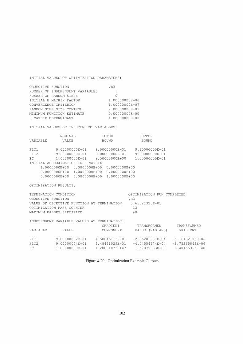
INITIAL VALUES OF OPTIMIZATION PARAMETERS:
OBJECTIVE FUNCTION VR3NUMBER OF INDEPENDENT VARIABLES 3NUMBER OF RANDOM STEPS 0INITIAL H MATRIX FACTOR 1.00000000E+00CONVERGENCE CRITERION 1.00000000E-07RANDOM STEP SIZE CONTROL 2.00000000E-01MINIMUM FUNCTION ESTIMATE 0.00000000E+00H MATRIX DETERMINANT 1.00000000E+00
INITIAL VALUES OF INDEPENDENT VARIABLES:
NOMINAL LOWER UPPERVARIABLE VALUE BOUND BOUND
P1T1 9.60000000E-01 9.00000000E-01 9.80000000E-01P1T2 9.60000000E-01 9.00000000E-01 9.80000000E-01EC 1.00000000E+01 9.50000000E+00 1.05000000E+01INITIAL APPROXIMATION TO H MATRIX
1.0000000E+00 0.0000000E+00 0.0000000E+000.0000000E+00 1.0000000E+00 0.0000000E+000.0000000E+00 0.0000000E+00 1.0000000E+00
OPTIMIZATION RESULTS:
TERMINATION CONDITION OPTIMIZATION RUN COMPLETEDOBJECTIVE FUNCTION VR3VALUE OF OBJECTIVE FUNCTION AT TERMINATION 5.65021325E-01OPTIMIZATION PASS COUNTER 13MAXIMUM PASSES SPECIFIED 40
INDEPENDENT VARIABLE VALUES AT TERMINATION:GRADIENT TRANSFORMED TRANSFORMED
VARIABLE VALUE COMPONENT VALUE (RADIANS) GRADIENT
P1T1 9.00000002E-01 4.50846113E-01 -2.86201981E-04 -5.16132196E-06P1T2 9.00000004E-01 5.48451029E-01 -4.44554674E-04 -9.75265843E-06EC 1.00000000E+01 1.28031073-147 1.57079633E+00 6.40155365-148
Figure 4.20.: Optimization Example Outputs
102
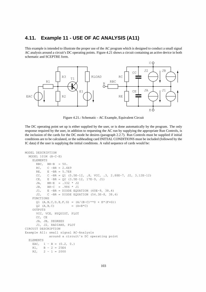
4.11. Example 11 - USE OF AC ANALYSIS (A11)
This example is intended to illustrate the proper use of the AC program which is designed to conduct a small signalAC analysis around a circuit’s DC operating points. Figure 4.21 shows a circuit containing an active device in bothschematic and SCEPTRE form.
@@I
e
e
e6
?
?
6
??
EAC
R1
R3T1
RLOAD
E1
R2
BRBC
RCCC
CE
RE
JA
J2 JB
J1
C
E
r
r
r
r r r r
rr
r rFigure 4.21.: Schematic - AC Example, Equivalent Circuit
The DC operating point set up is either supplied by the user, or is done automatically by the program. The onlyresponse required by the user, in addition to requesting the AC run by supplying the appropriate Run Controls, isthe inclusion of the cards for the DC mode he desires (paragraph 2.2.7). Run Controls must be supplied if initialconditions are to be calculated, or the subheading card INITIAL CONDITIONS must be included (followed by theIC data) if the user is supplying the initial conditions. A valid sequence of cards would be:
MODEL DESCRIPTIONMODEL 101M (B-C-E)
ELEMENTSRBC, BR-B = 50.RC, C -BR = 2.4E9RE, E -BR = 5.7E8CC, C -BR = Q1 (5.5E-12, .8, VCC, .3, 2.88E-7, J2, 3.12E-12)CE, E -BR = Q2 (3.5E-12, 17E-9, J1)JA, BR-E = .332 * J2JB, BR-C = .986 * J1J1, E -BR = DIODE EQUATION (60E-9, 38.4)J2, C -BR = DIODE EQUATION (54.3E-8, 38.4)
FUNCTIONSQ1 (A,B,C,D,E,F,G) = (A/(B-C)**D + E*(F+G))Q2 (A,B,C) = (A+B*C)
OUTPUTSVCC, VCE, NYQUIST, PLOTCC, CEJA, JB, DEGREESJ1, J2, RADIANS, PLOT
CIRCUIT DESCRIPTIONExample A11: small signal AC-Analysis
around a circuit’s DC operating pointELEMENTS
EAC, 1 - B = (0.2, 0.)R1, B - 2 = 25E4R2, 2 - 1 = 2000
103

R3, 2 - 3 = 11500RLOAD,3 - 4 = 100E1, 1 - 4 = -20T1, 2-3-1 = MODEL 101M
OUTPUTSVR2, VR3, COMPLEX, PLOT
RUN CONTROLSRUN INITIAL CONDITIONSPRINT EIGENVALUESPRINT EIGENVECTORSRUN ACINITIAL FREQUENCY = 1E5FINAL FREQUENCY = 1E6NUMBER FREQUENCY STEPS = 20TYPE FREQUENCY RUN = LINEAR
END
The automatic DC operating point set-up procedure results in the Initial Condition program, SIMIC, being writtenand executed. This is followed by one pass through the transient program, SIMTR, in order to deterinine the valuesof any elements, or outputs, that may be dependent on the initial conditions. Then, the AC analysis proceeds usingfixed resistor values, representing the DC operating points, instead of the original CLASS J9 diode sources. Theuser will receive a listing of these various DC results as follows:
OUTPUTS BEFORE AC RUN
VCCT1 -1.3023927E+01VCET1 3.6223429E-01CCT1 2.3449600E-12CET1 1.1243506E-09JAT1 -1.8027600E-07JBT1 6.5009336E-02J1T1 6.5932389E-02J2T1 -5.4300000E-07VR2 -4.0836859E-01VR3 1.2977793E+01
J9 SOURCE ’J1T1 ’ IS REPLACED BY RESISTOR= 0.3949750
J9 SOURCE ’J2T1 ’ IS REPLACED BY RESISTOR= 0.2400000E+13
LSNEW: COMPLEX EIGENVALUES
I REAL IMAGINARY MAGNITUDE
1 -0.65292E+10 0.00000E+00 0.65292E+102 -0.33353E+08 0.00000E+00 0.33353E+08
ATRACE = -0.6562516388467601E+10
EIGENVALUE SUM = -0.6562516388467599E+10 0.0000000000000000E+00
WHEN COMPARING A*S WITH S*LAMBDA, THE WORST ERROR OBTAINED WAS (-0.19073E-05, 0.00000E+00)WHEN MULTIPLYING MODAL MATRIX BY INVERSE MODAL MATRIX
WORST ERROR IN DIAGONAL TERM WAS ( 0.00000E+00, 0.00000E+00)WORST ERROR IN OFF-DIAGONAL TERM WAS ( 0.00000E+00, 0.00000E+00)
SINEW: MODAL MATRIX ... S
1 21 1.0000E+00 0.0000E+00 9.9999E-01 0.0000E+002 -2.0843E-03 0.0000E+00 3.9932E-03 0.0000E+00
SINEW: INVERSE MODAL MATRIX ...SI
1 21 6.5705E-01 0.0000E+00 -1.6454E+02 0.0000E+002 3.4296E-01 0.0000E+00 1.6454E+02 0.0000E+00
104
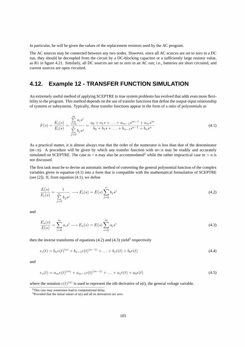
In particular, he will be given the values of the replacement resistors used by the AC program.
The AC sources may be connected between any two nodes. However, since all AC scurces are set to zero in a DCrun, they should be decoupled from the circuit by a DC-blocking capacitor or a sufficiently large resistor value,as R1 in figure 4.21. Similarly, all DC sources are set to zero in an AC run; i.e., batteries are short circuited, andcurrent sources are open circuited.
4.12. Example 12 - TRANSFER FUNCTION SIMULATION
An extremely useful method of applying SCEPTRE to true system problems has evolved that adds even more flexi-bility to the program. This method depends on the use of transfer functions that define the output-input relationshipof systems or subsystems. Typically, these transfer functions appear in the form of a ratio of polynomials as
F (s) =Eo(s)Ei(s)
=
m∑i=0
aisi
n∑j=0
bjsj=a0 + a1s+ . . .+ am−1s
m−1 + amsm
b0 + b1s+ . . .+ bn−1sn−1 + bnsn(4.1)
As a practical matter, it is almost always true that the order of the numerator is less than that of the denominator(m<n). A procedure will be given by which any transfer function with m<n may be readily and accuratelysimulated on SCEPTRE. The case m = n may also be accommodated2 while the rather impractical case m> n isnot discussed.
The first task must be to devise an automatic method of converting the general polynomial function of the complexvariables given in equation (4.1) into a form that is compatible with the mathematical formulation of SCEPTRE(see [2]). If, from equation (4.1), we define
E(s)Ei(s)
=1
n∑j=0
bjsj−→ Ei(s) = E(s)
n∑j=0
bjsj (4.2)
and
Eo(s)E(s)
=m∑i=0
aisi −→ Eo(s) = E(s)
m∑i=0
aisi (4.3)
then the inverse transforms of equations (4.2) and (4.3) yield3 respectively
ei(t) = bne(t)(n) + bn−1e(t)(n−1) + . . .+ b1e(t) + b0e(t) (4.4)
and
eo(t) = ame(t)(m) + am−1e(t)(m−1) + . . .+ a1e(t) + a0e(t) (4.5)
where the notatione(t)(n) is used to represent the nth derivative of e(t), the general voltage variable.2This case may sometimes lead to computational delay.3Provided that the initial values of e(t) and all its derivatives are zero.
105
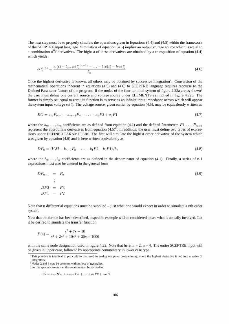
The next step must be to properly simulate the operations given in Equations (4.4) and (4.5) within the frameworkof the SCEPTRE input language. Simulation of equation (4.5) implies an output voltage source which is equal toa combination oTf derivatives. The highest of these derivatives are obtained by a transposition of equation (4.4)which yields
e(t)(n) =ei(t)− bn−1e(t)(n−1) − . . .− b1e(t)− b0e(t)
bn(4.6)
Once the highest derivative is known, all others may be obtained by successive integration4. Conversion of themathematical operations inherent in equations (4.5) and (4.6) to SCEPTRE language requires recourse to theDefined Parameter feature of the program. If the nodes of the four terminal system of figure 4.22a are as shown5
the user must define one current source and voltage source under ELEMENTS as implied in figure 4.22b. Theformer is simply set equal to zero; its function is to serve as an infinite input impedance across which will appearthe system input voltageei(t). The voltage source, given earlier by equation (4.5), may be equivalently written as
EO = amPm+1 + am−1Pm + . . .+ a1P2 + a0P1 (4.7)
where thea0, . . . , am coefficients are as defined from equation (4.1) and the defined ParametersP1, . . . , Pm+1
represent the appropriate derivatives from equation (4.5)6. In addition, the user must define two types of expres-sions under DEFINED PARAMETERS. The first will simulate the highest order derivative of the system whichwas given by equation (4.6) and is here written equivalently as
DPn = (V JI − bn−1Pn − . . .− b1P2− b0P1)/bn (4.8)
where theb0, . . . , bn coefficients are as defined in the denominator of equation (4.1). Finally, a series of n-1expressions must also be entered in the general form
DPn−1 = Pn (4.9)...
DP2 = P3DP1 = P2
Note that n differential equations must be supplied – just what one would expect in order to simulate a nth ordersystem.
Now that the format has been described, a specific example will be considered to see what is actually involved. Letit be desired to simulate the transfer function
F (s) =s2 + 7s− 10
s4 + 2s3 + 10s2 + 20s+ 1000
with the same node designation used in figure 4.22. Note that here m = 2, n = 4. The entire SCEPTRE input willbe given in upper case, followed by appropriate commentary in lower case type.
4This practice is identical in principle to that used in analog computer programming where the highest derivative is fed into a series ofintegrators.
5Nodes 2 and 8 may be common without loss of generality.6For the special case m = n, this relation must be revised to
EO = amDPm + am−1Pm + . . .+ a1P2 + a0P1
106
7
82
1
F(s)
7
8
1
2
JI EO
+
-
b)a)65.fig
Figure 4.22.: A Transfer Function Block and the Equivalent SCEPTRE Representation
ELEMENTSJI, 1-2 = 0E0, 8-7 = X1 (DP2+7.*P2-10.*P1) from equation (4.7)DEFINED PARAMETERSDP4 = X2 ((VJI-2.*P4-10.*P3-200.*P2-1000.*P1)/1)
from equation (4.8)
DP3 = X3 (P4) from equation (4.9)DP2 = X4 (P3)DP1 = X4 (P2)P1 = 0 these establish initial values.P2 = 0 They may be omitted, and the onlyP3 = 0 consequence will be a seriesP4 = 0 of warning messages.
It is clear that, if a particular system requires two or more transfer functions of the above type, the user must repeatthe procedure for each one. If there are very many transfer functions involved, or if those that are involved are ofhigher order, the input task becomes a bit tedious and error prone. The remedy for this, of course, is the storedmodel of SCEPTRE. It is suggested that the user store on his permanent tape one model for each degree transferfunction of interest7. The process is simple and need be done only once. An example of the storage procedure fora general second order transfer function will be given. This model will then be called for use as a specific secondorder function. Consider permanent storage of the following with m = 2, n = 2:
F2(s) =a2s
2 + a1s+ a0
b2s2 + b1s+ b0
The required cards are
MODEL DESCRIPTIONMODEL 2ORDER (PERM) (A-B-C-D)ELEMENTSJI, A-B = 0E0, D-C = X1 (PA2*DP2 + PA1*P2 + PAO*P1)DEFINED PARAMETERSDP2 = X2 ((VJI - PB1*P2 - PBO*P1)/PB2)DP1 = X3 (P2)PAO = 0, PA1 = 0, PA2 = 0PBO = 0, PB1 = 0, PB2 = 0P1=0, P2=0
7A higher order model could be stored and degenerated to one of the desired order by proper manipulation of Defined Parameters. Themethod suggested here uses less computer solution time, fewer Defined Parameters, and is less complicated.
107
Here the Defined Parameters are named as PAO, ...., PBO, .... to correspond with coefficientsa0, . . . , b0, . . .. P1and P2 serve as the dependent variables of the two differential equations. The model is general in that any of thecoefficients can be changed (when the model is called) from the originally assigned zero values. It should be notedthat, even though this model is stored with provision for the case m = n, this will not be the case actually usedunless parameter PA2 is made non-zero in the model call.
Now that the model has been stored in general second order form, the desired coefficients needed to representa specific second order transfer function can be supplied when the model is called out for use under CIRCUITDESCRIPTION.
If it desired to simulate
Eo(s)Ei(s)
=10s+ 4
s2 + .7s+ 5
with the nodes as labeled in figure 4.22a, an appropriate entry sequence would be
CIRCUIT DESCRIPTIONELEMENTS
.....G2, 1-2-7-8 = MODEL 2ORDER (PERM, CHANGE PAO = 4,
PA1 = 10, PBO = 5, PB1 = 0.7, PB2 = 1)
The same model could be called repeatedly to represent many second order transfer functions with arbitrary coeffi-cients. The procedure is even simpler to simulate ideal amplifiers, summing junctions and limit functions (see [3]).The ability of SCEPTRE to perform these operations now qualify it as a tool for systems analysis. When one con-bines this with its unmatched capability for nonlinear circuit analysis, its potential for the solution of large systemsthat can be broken down into non-linear circuitry and linear subsystems becomes clear.
108
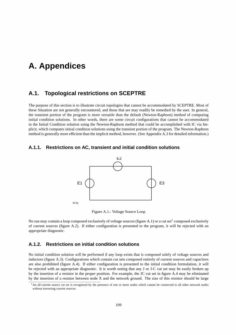
A. Appendices
A.1. Topological restrictions on SCEPTRE
The purpose of this section is to illustrate circuit topologies that cannot be accommodated by SCEPTRE. Most ofthese Situation are not generally encountered, and those that are may readily be remedied by the user. In general,the transient portion of the program is more versatile than the default (Newton-Raphson) method of computinginitial condition solutions. In other words, there are some circuit configurations that cannot be accommodatedin the Initial Condition solution using the Newton-Raphson method that could be accomplished with IC via Im-plicit, which computes initial condition solutions using the transient portion of the program. The Newton-Raphsonmethod is generally more efficient than the implicit method, however. (See Appendix A.3 for detailed information.)
A.1.1. Restrictions on AC, transient and initial condition solutions
E1
E2
66.fig
E3
Figure A.1.: Voltage Source Loop
No run may contain a loop composed exclusively of voltage sources (figure A.1) or a cut set1 composed exclusivelyof current sources (figure A.2). If either configuration is presented to the program, it will be rejected with anappropriate diagnostic.
A.1.2. Restrictions on initial condition solutions
No initial condition solution will be performed if any loop exists that is composed solely of voltage sources andinductors (figure A.3). Configurations which contain cut sets composed entirely of current sources and capacitorsare also prohibited (figure A.4). If either configuration is presented to the initial condition formulation, it willbe rejected with an appropriate diagnostic. It is worth noting that any J or J-C cut set may be easily broken upby the insertion of a resistor in the proper position. For example, the JC cut set in figure A.4 may be eliminatedby the insertion of a resistor between node X and the network ground. The size of this resistor should be large
1An all-current source cut set is recognized by the presence of one or more nodes which cannot be connected to all other network nodeswithout traversing current sources.
109
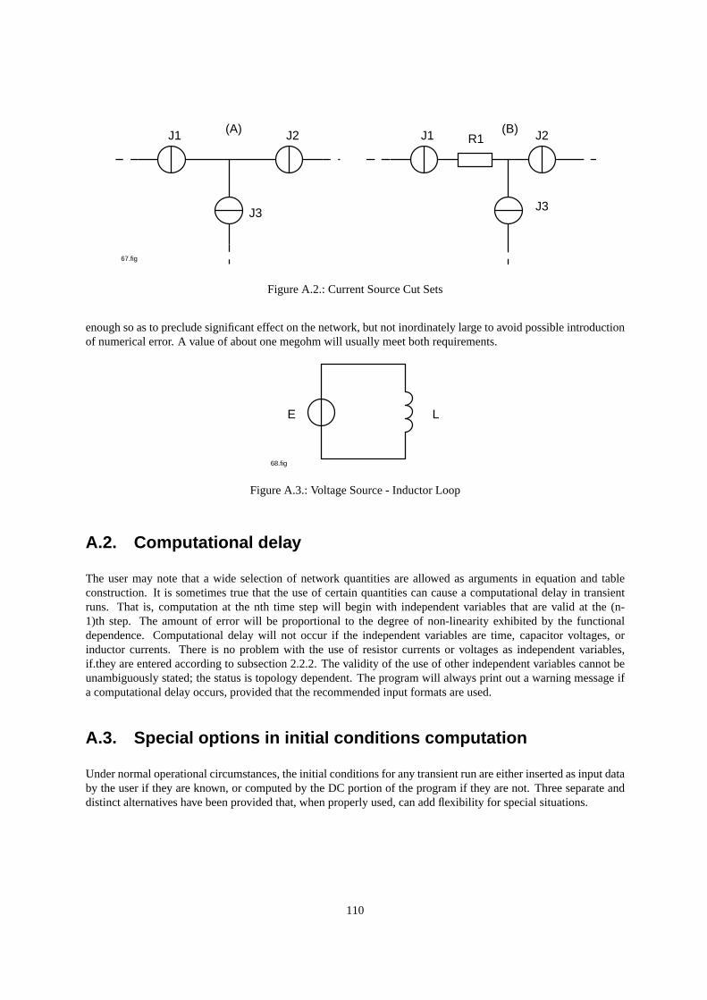
J1 J2
J3
67.fig
J3
R1 J2J1(A) (B)
Figure A.2.: Current Source Cut Sets
enough so as to preclude significant effect on the network, but not inordinately large to avoid possible introductionof numerical error. A value of about one megohm will usually meet both requirements.
E L
68.fig
Figure A.3.: Voltage Source - Inductor Loop
A.2. Computational delay
The user may note that a wide selection of network quantities are allowed as arguments in equation and tableconstruction. It is sometimes true that the use of certain quantities can cause a computational delay in transientruns. That is, computation at the nth time step will begin with independent variables that are valid at the (n-1)th step. The amount of error will be proportional to the degree of non-linearity exhibited by the functionaldependence. Computational delay will not occur if the independent variables are time, capacitor voltages, orinductor currents. There is no problem with the use of resistor currents or voltages as independent variables,if.they are entered according to subsection 2.2.2. The validity of the use of other independent variables cannot beunambiguously stated; the status is topology dependent. The program will always print out a warning message ifa computational delay occurs, provided that the recommended input formats are used.
A.3. Special options in initial conditions computation
Under normal operational circumstances, the initial conditions for any transient run are either inserted as input databy the user if they are known, or computed by the DC portion of the program if they are not. Three separate anddistinct alternatives have been provided that, when properly used, can add flexibility for special situations.
110
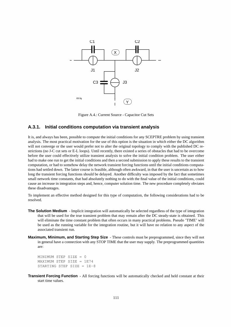
69.fig
J1
X
J3
Y
C3
C1 C2
J2
Figure A.4.: Current Source - Capacitor Cut Sets
A.3.1. Initial conditions computation via transient analysis
It is, and always has been, possible to compute the initial conditions for any SCEPTRE problem by using transientanalysis. The most practical motivation for the use of this option is the situation in which either the DC algorithmwill not converge or the user would prefer not to alter the original topology to comply with the published DC re-strictions (no J-C cut sets or E-L loops). Until recently, there existed a series of obstacles that had to be overcomebefore the user could effectively utilize transient analysis to solve the initial condition problem. The user eitherhad to make one run to get the initial conditions and then a second submission to apply these results to the transientcomputation, or had to somehow delay the network transient forcing functions until the initial conditions computa-tions had settled down. The latter course is feasible, although often awkward, in that the user is uncertain as to howlong the transient forcing functions should be delayed. Another difficulty was imposed by the fact that sometimessmall network time constants, that had absolutely nothing to do with the final value of the initial conditions, couldcause an increase in integration steps and, hence, computer solution time. The new procedure completely obviatesthese disadvantages.
To implement an effective method designed for this type of computation, the following considerations had to beresolved.
The Solution Medium - Implicit integration will automatically be selected regardless of the type of integrationthat will be used for the true transient problem that may remain after the DC steady-state is obtained. Thiswill eliminate the time constant problem that often occurs in many practical problems. Pseudo ’TIME’ willbe used as the running variable for the integration routine, but it will have no relation to any aspect of theassociated transient run.
Maximum, Minimum, and Starting Step Size - These controls must be preprogrammed, since they will notin general have a connection with any STOP TIME that the user may supply. The preprogrammed quantitiesare:
MINIMUM STEP SIZE = 0MAXIMUM STEP SIZE = 1E74STARTING STEP SIZE = 1E-8
Transient Forcing Function - All forcing functions will be automatically checked and held constant at theirstart time values.
111
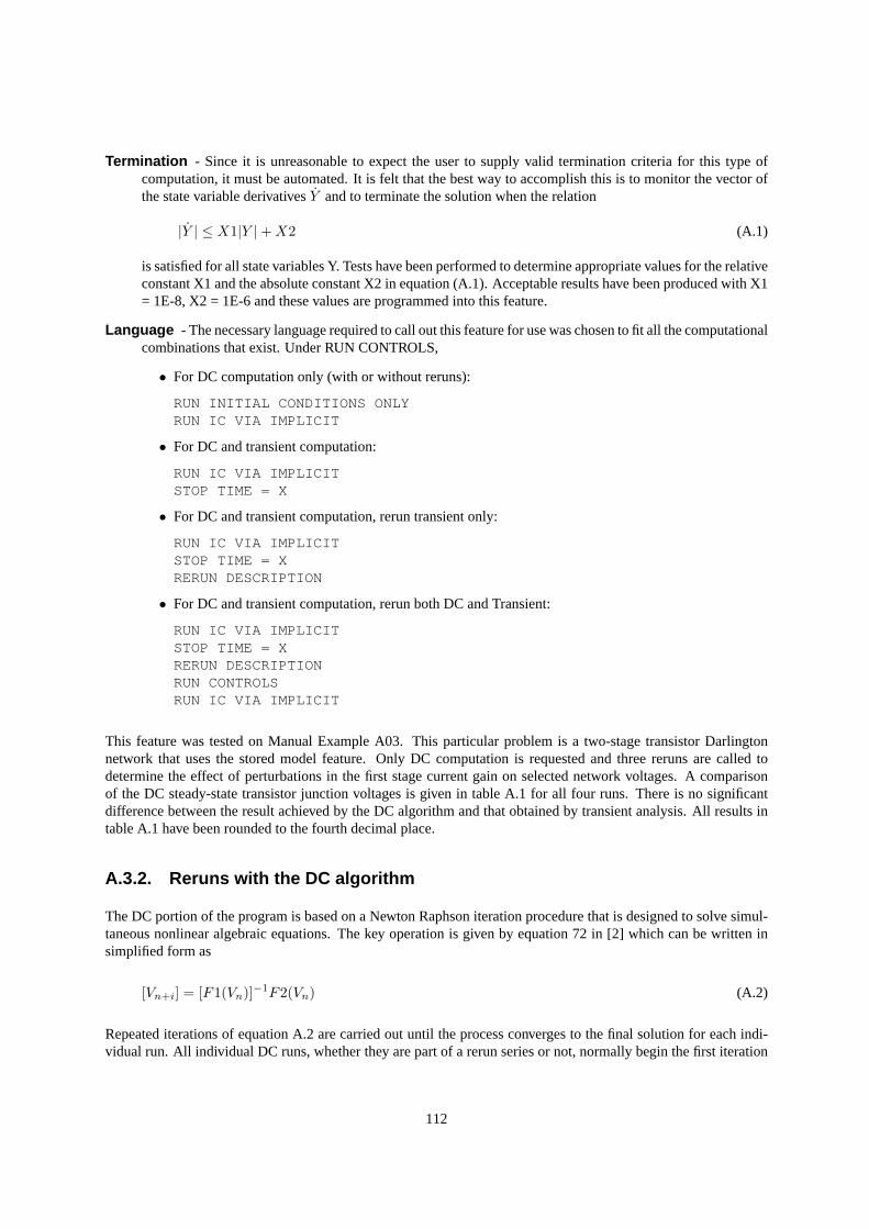
Termination - Since it is unreasonable to expect the user to supply valid termination criteria for this type ofcomputation, it must be automated. It is felt that the best way to accomplish this is to monitor the vector ofthe state variable derivativesY and to terminate the solution when the relation
|Y | ≤ X1|Y |+X2 (A.1)
is satisfied for all state variables Y. Tests have been performed to determine appropriate values for the relativeconstant X1 and the absolute constant X2 in equation (A.1). Acceptable results have been produced with X1= 1E-8, X2 = 1E-6 and these values are programmed into this feature.
Language - The necessary language required to call out this feature for use was chosen to fit all the computationalcombinations that exist. Under RUN CONTROLS,
• For DC computation only (with or without reruns):
RUN INITIAL CONDITIONS ONLYRUN IC VIA IMPLICIT
• For DC and transient computation:
RUN IC VIA IMPLICITSTOP TIME = X
• For DC and transient computation, rerun transient only:
RUN IC VIA IMPLICITSTOP TIME = XRERUN DESCRIPTION
• For DC and transient computation, rerun both DC and Transient:
RUN IC VIA IMPLICITSTOP TIME = XRERUN DESCRIPTIONRUN CONTROLSRUN IC VIA IMPLICIT
This feature was tested on Manual Example A03. This particular problem is a two-stage transistor Darlingtonnetwork that uses the stored model feature. Only DC computation is requested and three reruns are called todetermine the effect of perturbations in the first stage current gain on selected network voltages. A comparisonof the DC steady-state transistor junction voltages is given in table A.1 for all four runs. There is no significantdifference between the result achieved by the DC algorithm and that obtained by transient analysis. All results intable A.1 have been rounded to the fourth decimal place.
A.3.2. Reruns with the DC algorithm
The DC portion of the program is based on a Newton Raphson iteration procedure that is designed to solve simul-taneous nonlinear algebraic equations. The key operation is given by equation 72 in [2] which can be written insimplified form as
[Vn+i] = [F1(Vn)]−1F2(Vn) (A.2)
Repeated iterations of equation A.2 are carried out until the process converges to the final solution for each indi-vidual run. All individual DC runs, whether they are part of a rerun series or not, normally begin the first iteration
112

Rerun # Variable via DC analysis via TR analysisMaster VCET1 0.3382 0.3382Run VCCT1 -8.9377 -8.9377
VCET2 0.4422 0.4422VCCT2 -8.8227 -8.8226
First VCET1 0.3377 0.3377Rerun VCCT1 -8.9456 -8.9458
VCET2 0.4416 0.4416VCCT2 -8.8381 -8.8383
Second VCET1 0.3370 0.3369Rerun VCCT1 -8.9570 -8.9572
VCET2 0.4408 0.4408VCCT2 -8.8603 -8.8605
Third VCET1 0.3363 0.3362Rerun VCCT1 -8.9680 -8.9680
VCET2 0.4399 0.4399VCCT2 -8.8813 -8.8814
Table A.1.: Comparison of DC results
with the left side of equation A.2 set to zero. The average network usually converges to a final solution in anywherefrom 10 to 25 iterations.
It is usually true that, when a series of DC only reruns are to be made, the overall circuit differs just slightly inelement value from one rerun to the next. It follows then that the final solution will also not vary greatly from rerunto rerun. In circumstances of this type it is often likely that convergence of a given rerun could be significantlyspeeded if the final results of a preceding run were used as the starting point. Example A03 of the manual canbe used again as an illustration. When the master run and each of the three associated reruns were started atzero voltage, all four runs converged in 11 passes. The same problem was repeated with each of the three rerunsbegun with the voltages with which its predecessor finished. Convergence was then obtained in four passes foreach of the reruns and there was no difference in accuracy. Other tests have been made with comparable results.The attractiveness of this feature will, of course, be proportional to the number of DC reruns that are to be made.Significant computer solution time will be saved only if a significant number of reruns are used.
Two variants of this feature are allowed. The first is if all reruns are to begin with the final voltages of the masterrun. In that case, the required language is
RUN CONTROLSRUN INITIAL CONDITIONS ONLYIC FOR RERUNS = MASTER RESULTSRERUN DESCRIPTION (N)
The second version of this feature allows all reruns to begin with the final voltages of the run preceding it. The (n+ 1)th rerun would start with the final voltages of the nth rerun. The required language then becomes
RUN CONTROLSRUN INITIAL CONDITIONS ONLYIC FOR RERUNS = PRECEDING RESULTSRERUN DESCRIPTION (N)
It is possible to combine this feature with DC via Transient feature described in the preceding section. The languageis
113

RUN CONTROLSRUN INITIAL CONDITIONS ONLYRUN IC VIA IMPLICITIC FOR RERUNS = either formRERUN DESCRIPTION (N)
Note that in all possible cases the necessary call is inserted under RUN CONTROLS of the master run and neverunder RERUN DESCRIPTION.
A.3.3. Optional initial conditions for transient reruns
The third alternative for initial conditions is a method that has some of the characteristics of the other two. It issimilar to the method of subsection A.3.1, in that it utilizes transient analysis and is similar to the subsection A.3.2technique because it applies to reruns only. It offers the user the capability of starting any transient rerun with thestate variable values that existed at the end of a previous transient run. Consider the situation in which the effectof a series of pulses applied to a given network is to be ascertained. If the phenomena connected with each pulseis such that it affects some network parameter (say transistor current gain) that, in turn, affects the quiescent pointof the network, it may be advantageous to run the entire problem as a master run with a series of associated reruns.The state variable values that exist at the end of each individual transient run will be transferred to the beginningof the next run without any intervening analysis.
The required language is identical to that given in the preceding section. If the master run final values are to serveas the starting point for all associated reruns, enter under RUN CONTROLS:
IC FOR RERUNS = MASTER RESULTS
If all runs are to begin with the final values of the previous run, enter
IC FOR RERUNS = PRECEDING RESULTS
There is no danger of ambiguity that may be implied by the identical language. The feature in the previous sectionis distinguished from this one by the fact that it will also contain the statement RUN INITIAL CONDITIONSONLY.
A.4. Specified print interval
The basic output format of SCEPTRE supplies printed output at every successful step taken by the integrationmethod up to a default maximum of 1000 points. If more than 1000 steps are taken, that number is divided bythe smallest integer, n, such that every nth step is printed out and no more than 1000 points would be output. Ifa given run took 2115 steps (n here is 3), 705 points or every third step would be output. No attempt is made tospace the print increments; if it happens that many steps are taken in the first half of a run and comparatively fewin the last half the printed output will be spaced accordingly. In most cases, this is desirable and the basic formatwas chosen for that reason. In some situations, a different format can be attractive and has been made available.The objective of the optional Specified Print Interval feature is to enable the user to precisely control the numberof printed output points and to allow them to be more selectively chosen. The user may supply the time interval atwhich print points are desired and only those solution points that fall on or immediately after integer multiples ofthe specified interval will be printed. Assume, for example that a transient problem is run to a STOP TIME = 800,and that the first few solution points are at the following times: 0, 2, 4, 6, 8, 10, 14, 18, 22......... Assume also that
114

the user has specified a print interval of 10. In that case printed output would appear at times 0, 10, 22........ andthe number of print points would equal STOP TIME divided by PRINT INTERVAL ( = 80 in addition to the oneat time = 0). The only situation in which the number of output print points would differ from the above relation isthe rather uncommon situation in which the specified print interval is smaller than the step sizes actually taken.
This feature is optional and is activated by the entry
PRINT INTERVAL = number
under the RUN CONTROLS section. This printed series will appear in addition to the normal output. If only thisprinted series is desired, the normal printed output format may be suppressed by the entry
MAXIMUM PRINT POINTS = 0
A.5. Composite plots
The standard plot format with SCEPTRE has always been one dependent variable plotted against an independentvariable with automatic scaling supplied for both the abscissa and ordinate. The plots were output in machine plotformat with all abscissas having physical lengths of 10 inches and ordinates of 8-1/2 inches. A summary of allquantities that may be plotted is given in Manual subsection 2.2.4.
A specialized plot format has been added in which up to nine quantities may be plotted against a common abscissa.The ordinate values for each variable are separately scaled in order to preserve resolution and unique characters areused to represent each quantity. Use of this feature requires that all of the quantities that are to be plotted togetherbe requested on the same card under OUTPUTS followed by a specific plot name. The plots illustrated in figureA.5 were obtained with the following entries:
OUTPUTSPX, PY, PZ, XSTPSZ, PLOT GREEN
RUN CONTROLSPLOT INTERVAL = 1STOP TIME = 80
Here the four quantities PX, PY, PZ and XSTPSZ are requested, together with a specific plot name of ’GREEN’.Any alphanumeric combination not exceeding six characters could as well have been used to designate the plotname. Any of the dependent variables could have been renamed according to the format given, in Manual subsec-tion 2.2.4 and the number of composite plots is restricted only by the program limit of 100 output quantities. Theonly independent variable allowed for these plots, however, is TIME. Use of this feature does not affect the printedoutput format in any way.
Provision has also been made to allow the user to control the physical length of any composite plot. The numberof pages over which the length of any of these plots are spread depends upon the problem duration (STOP TIME)and a user supplied quantity called PLOT INTERVAL. The number of lines covered by the plot will equal theSTOP TIME divided by the PLOT INTERVAL. For the System/360, 59 lines will fill one page. Therefore, a STOPTIME of 1000 and a PLOT INTERVAL of 5 will require 200 lines and lead to a plot of about four pages in length.The PLOT INTERVAL entry is supplied under RUN CONTROLS and only one such entry will be recognizedregardless of the number of composite plots requested. The user is free to control the length of any single plottedentry by simply supplying a plot name and a PLOT INTERVAL entry.
115
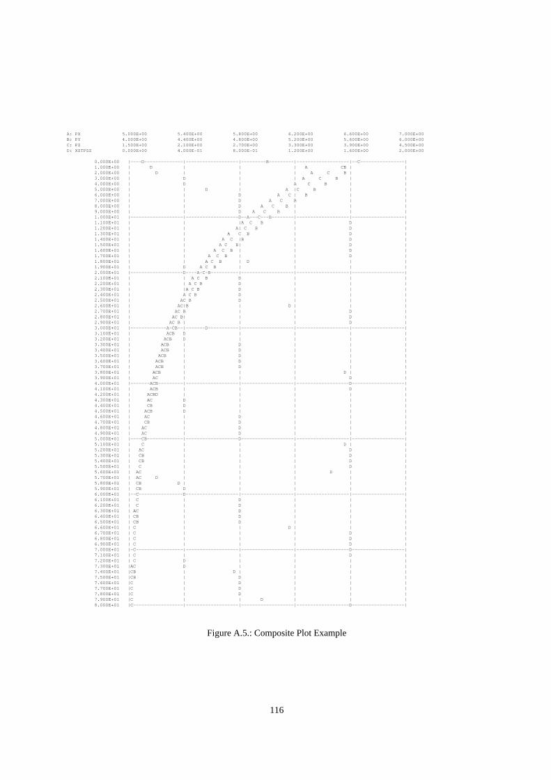
A: PX 5.000E+00 5.400E+00 5.800E+00 6.200E+00 6.600E+00 7.000E+00B: PY 4.000E+00 4.400E+00 4.800E+00 5.200E+00 5.600E+00 6.000E+00C: PZ 1.500E+00 2.100E+00 2.700E+00 3.300E+00 3.900E+00 4.500E+00D: XSTPSZ 0.000E+00 4.000E-01 8.000E-01 1.200E+00 1.600E+00 2.000E+00
0.000E+00 |----D--------------|-------------------|---------B---------|-------------------|--C----------------|1.000E+00 | D | | | A CB | |2.000E+00 | D | | | A C B | |3.000E+00 | D | | A C B | |4.000E+00 | D | A C B | |5.000E+00 | | D | A |C B | |6.000E+00 | | D A C | B | |7.000E+00 | | D A C B | |8.000E+00 | | D A C B | | |9.000E+00 | | D A C B | | |1.000E+01 |-------------------|-------------------D--A---C---B--------|-------------------|-------------------|1.100E+01 | | |A C B | D |1.200E+01 | | A| C B | D |1.300E+01 | | A C B | D |1.400E+01 | | A C |B | D |1.500E+01 | | A C B| | D |1.600E+01 | | A C B | | D |1.700E+01 | | A C B | | D |1.800E+01 | | A C B | D | | |1.900E+01 | D A C B | | | |2.000E+01 |-------------------D----A-C-B----------|-------------------|-------------------|-------------------|2.100E+01 | | A C B D | | |2.200E+01 | | A C B D | | |2.300E+01 | |A C B D | | |2.400E+01 | A C B D | | |2.500E+01 | AC B D | | |2.600E+01 | AC|B | D | | |2.700E+01 | AC B | | D |2.800E+01 | AC B| | | D |2.900E+01 | AC B | | | D |3.000E+01 |-------------A-CB--|-------D-----------|-------------------|-------------------|-------------------|3.100E+01 | ACB D | | | |3.200E+01 | ACB D | | | |3.300E+01 | ACB | D | | |3.400E+01 | ACB | D | | |3.500E+01 | ACB | D | | |3.600E+01 | ACB | D | | |3.700E+01 | ACB | D | | |3.800E+01 | ACB | | | D | |3.900E+01 | AC | | | D |4.000E+01 |-------ACB---------|-------------------|-------------------|-------------------D-------------------|4.100E+01 | ACB | | | D |4.200E+01 | ACBD | | | | |4.300E+01 | AC D | | | |4.400E+01 | CB D | | | |4.500E+01 | ACB D | | | |4.600E+01 | AC | D | | |4.700E+01 | CB | D | | |4.800E+01 | AC | D | | |4.900E+01 | AC | D | | |5.000E+01 |----CB-------------|-------------------D-------------------|-------------------|-------------------|5.100E+01 | C | | | D | |5.200E+01 | AC | | | D |5.300E+01 | CB | | | D |5.400E+01 | CB | | | D |5.500E+01 | C | | | D |5.600E+01 | AC | | | D | |5.700E+01 | AC D | | | | |5.800E+01 | CB D | | | | |5.900E+01 | CB D | | | |6.000E+01 |--C----------------D-------------------|-------------------|-------------------|-------------------|6.100E+01 | C | D | | |6.200E+01 | C | D | | |6.300E+01 | AC | D | | |6.400E+01 | CB | D | | |6.500E+01 | CB | D | | |6.600E+01 | C | | D | | |6.700E+01 | C | | | D |6.800E+01 | C | | | D |6.900E+01 | C | | | D |7.000E+01 |-C-----------------|-------------------|-------------------|-------------------D-------------------|7.100E+01 | C | | | D |7.200E+01 | C D | | | |7.300E+01 |AC D | | | |7.400E+01 |CB | D | | | |7.500E+01 |CB | D | | |7.600E+01 |C | D | | |7.700E+01 |C | D | | |7.800E+01 |C | D | | |7.900E+01 |C | | D | | |8.000E+01 |C------------------|-------------------|-------------------|-------------------D-------------------|
Figure A.5.: Composite Plot Example
116
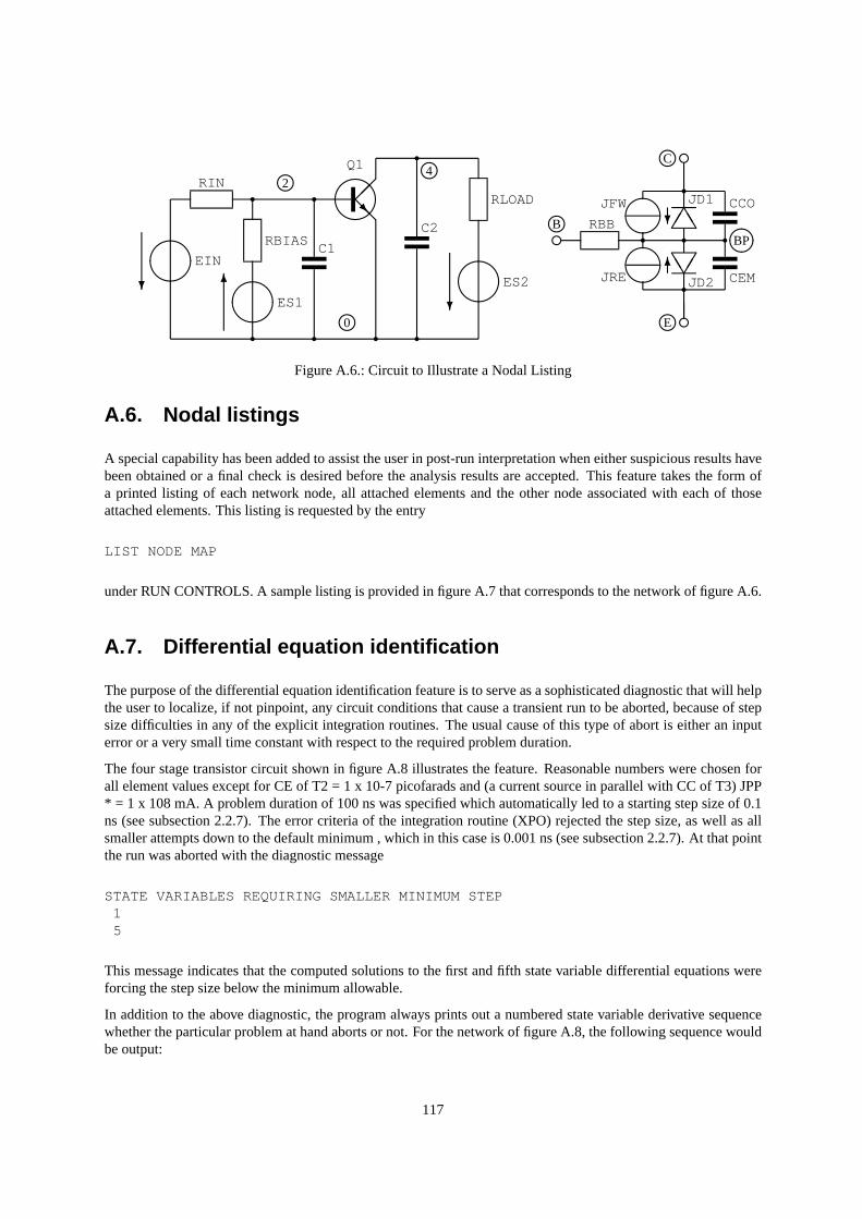
TT
TT
e
e
e r r r
@@R
? 6
?
?
6
RBB
CCO
CEM
JD1
JD2JRE
JFW
ES2
RLOAD
C2
Q1
C1
ES1
RBIAS
RIN
EIN
r
r r
r r r
rj jj
j
j
BP
C
E
B
42
j0
r
r
Figure A.6.: Circuit to Illustrate a Nodal Listing
A.6. Nodal listings
A special capability has been added to assist the user in post-run interpretation when either suspicious results havebeen obtained or a final check is desired before the analysis results are accepted. This feature takes the form ofa printed listing of each network node, all attached elements and the other node associated with each of thoseattached elements. This listing is requested by the entry
LIST NODE MAP
under RUN CONTROLS. A sample listing is provided in figure A.7 that corresponds to the network of figure A.6.
A.7. Differential equation identification
The purpose of the differential equation identification feature is to serve as a sophisticated diagnostic that will helpthe user to localize, if not pinpoint, any circuit conditions that cause a transient run to be aborted, because of stepsize difficulties in any of the explicit integration routines. The usual cause of this type of abort is either an inputerror or a very small time constant with respect to the required problem duration.
The four stage transistor circuit shown in figure A.8 illustrates the feature. Reasonable numbers were chosen forall element values except for CE of T2 = 1 x 10⁻⁷ picofarads and (a current source in parallel with CC of T3) JPP* = 1 x 10⁸ mA. A problem duration of 100 ns was specified which automatically led to a starting step size of 0.1ns (see subsection 2.2.7). The error criteria of the integration routine (XPO) rejected the step size, as well as allsmaller attempts down to the default minimum , which in this case is 0.001 ns (see subsection 2.2.7). At that pointthe run was aborted with the diagnostic message
STATE VARIABLES REQUIRING SMALLER MINIMUM STEP15
This message indicates that the computed solutions to the first and fifth state variable differential equations wereforcing the step size below the minimum allowable.
In addition to the above diagnostic, the program always prints out a numbered state variable derivative sequencewhether the particular problem at hand aborts or not. For the network of figure A.8, the following sequence wouldbe output:
117
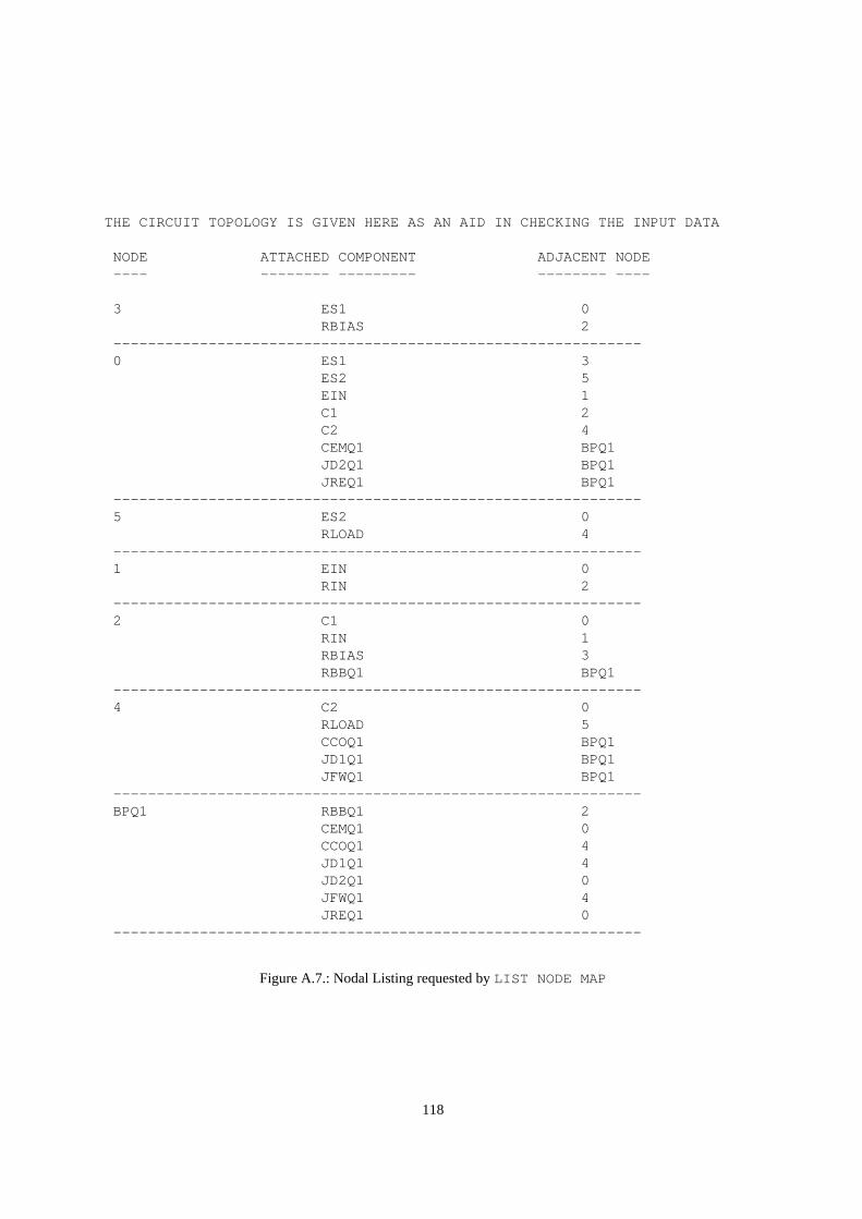
THE CIRCUIT TOPOLOGY IS GIVEN HERE AS AN AID IN CHECKING THE INPUT DATA
NODE ATTACHED COMPONENT ADJACENT NODE---- -------- --------- -------- ----
3 ES1 0RBIAS 2
-------------------------------------------------------------0 ES1 3
ES2 5EIN 1C1 2C2 4CEMQ1 BPQ1JD2Q1 BPQ1JREQ1 BPQ1
-------------------------------------------------------------5 ES2 0
RLOAD 4-------------------------------------------------------------1 EIN 0
RIN 2-------------------------------------------------------------2 C1 0
RIN 1RBIAS 3RBBQ1 BPQ1
-------------------------------------------------------------4 C2 0
RLOAD 5CCOQ1 BPQ1JD1Q1 BPQ1JFWQ1 BPQ1
-------------------------------------------------------------BPQ1 RBBQ1 2
CEMQ1 0CCOQ1 4JD1Q1 4JD2Q1 0JFWQ1 4JREQ1 0
-------------------------------------------------------------
Figure A.7.: Nodal Listing requested byLIST NODE MAP
118
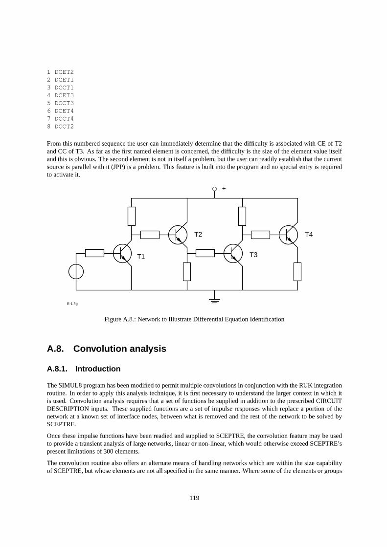
1 DCET22 DCET13 DCCT14 DCET35 DCCT36 DCET47 DCCT48 DCCT2
From this numbered sequence the user can immediately determine that the difficulty is associated with CE of T2and CC of T3. As far as the first named element is concerned, the difficulty is the size of the element value itselfand this is obvious. The second element is not in itself a problem, but the user can readily establish that the currentsource is parallel with it (JPP) is a problem. This feature is built into the program and no special entry is requiredto activate it.
+
T1
T2
T3
T4
E-1.fig
Figure A.8.: Network to Illustrate Differential Equation Identification
A.8. Convolution analysis
A.8.1. Introduction
The SIMUL8 program has been modified to permit multiple convolutions in conjunction with the RUK integrationroutine. In order to apply this analysis technique, it is first necessary to understand the larger context in which itis used. Convolution analysis requires that a set of functions be supplied in addition to the prescribed CIRCUITDESCRIPTION inputs. These supplied functions are a set of impulse responses which replace a portion of thenetwork at a known set of interface nodes, between what is removed and the rest of the network to be solved bySCEPTRE.
Once these impulse functions have been readied and supplied to SCEPTRE, the convolution feature may be usedto provide a transient analysis of large networks, linear or non-linear, which would otherwise exceed SCEPTRE’spresent limitations of 300 elements.
The convolution routine also offers an alternate means of handling networks which are within the size capabilityof SCEPTRE, but whose elements are not all specified in the same manner. Where some of the elements or groups
119

of elements are already described by their responses in the time domain, or are described by their responses in thefrequency domain and conversion to time domain is possible, then the convolution approach might save manualcalculation in preparing the network for analysis.
The larger context involving convolution is described in Section A.8.2. The type of non-linear network which isamenable to this approach is described in section A.8.3. The theory associated with the convolution mode withinSCEPTRE is given in section A.8.4, A.8.5, and A.8.6.
The required impulse response functions are assumed to reside on a disk file. Instructions and formats required forpreparing such a file are given in section A.8.7. The circuit description preparation required for the convolutionmode is also described in Table 2.2 of section 2.2.2, and in example 4.6.
A.8.2. Mixed-domain approach
The convolution feature is an integral portion of a more general technique designed primarily to permit a transientanalysis of a certain class of large non-linear networks. The major steps in the approach are:
1. Partition the network into two parts (see section A.8.3).
2. Use a frequency-domain program capable of solving a large linear network to determine the driving- pointand transfer immittance functions, H(ω), at the interface terminals.
3. Find the equivalent impulse response functions, h(t), in the time domain by using Fourier inversion.
4. Model these impulse response functions as either impedances or admittances. The impedance (admittance)model assumes that a removed portion of an existing circuit is characterized at the interface by a Theveninvoltage source (Norton current source) and a driving-point impedance (admittance).
5. Describe these time-domain functions in a way acceptable to SCEPTRE.
6. Solve the remaining moderate-size sub-network containing the nonlinearities, and include these impulseresponse functions using SCEPTRE with its convolution capability.
Step 1 is accomplished manually at the discretion of the user. Step 2 may be accomplished using any auxiliary ACanalysis program which is capable of providing the desired immittance functions. Step 3 is done using any off-lineprogram which can process the AC outputs and supply the necessary inverse Fourier Transforms. Steps 4, 5 and 6represent the convolution analysis portion of the overall approach.
The ability to do Steps 4, 5, and 6 is the key to this method of analysis. The problem of modeling the time functionsand processing them in synchronism with SCEPTRE was solved by observing that these functions form the impulseresponse matrix for the removed circuitry as seen by the original network across the appropriate interface terminals.Therefore, in the impedance mode, the time function of the voltage across any pair of interface terminals can beobtained by convolving the appropriate impedance function with the time function describing the current flowingthrough the two terminals. Similarly, in the admittance mode, the current flowing through the terminal can beobtained by convolving the voltage function, across the terminals, with the appropriate admittance function.
SCEPTRE calculates currents and voltages, for a given configuration, as functions of time. Therefore, in order tocalculate present values, it was necessary that the convolution routine be written so that, in the impedance mode(admittance mode), it uses past history of the current(voltage) to estimate the present value of current (voltage),which in turn will yield the required terminal-to-terminal voltage (current). It then updates the current and voltagetables and repeats the procedures for the next time step.
120
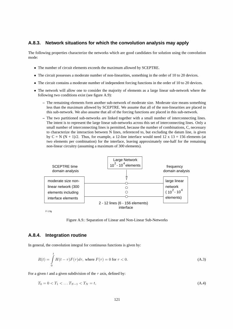
A.8.3. Network situations for which the convolution analysis may apply
The following properties characterize the networks which are good candidates for solution using the convolutionmode:
• The number of circuit elements exceeds the maximum allowed by SCEPTRE.
• The circuit possesses a moderate number of non-linearities, something in the order of 10 to 20 devices.
• The circuit contains a moderate number of independent forcing functions in the order of 10 to 20 devices.
• The network will allow one to consider the majority of elements as a large linear sub-network where thefollowing two conditions exist (see figure A.9):
– The remaining elements form another sub-network of moderate size. Moderate size means somethingless than the maximum allowed by SCEPTRE. We assume that all of the non-linearities are placed inthis sub-network. We also assume that all of the forcing functions are placed in this sub-network.
– The two partitioned sub-networks are linked together with a small number of interconnecting lines.The intent is to represent the large linear sub-networks across this set of interconnecting lines. Only asmall number of interconnecting lines is permitted, because the number of combinations, C, necessaryto characterize the interaction between N lines, referenced to, but excluding the datum line, is givenby C = N (N + 1)/2. Thus, for example, a 12-line interface would need 12 x 13 = 156 elements (attwo elements per combination) for the interface, leaving approximately one-half for the remainingnon-linear circuitry (assuming a maximum of 300 elements).
10 10-2 4
10 10-2 4
elements
Large Network
moderate size non-
linear network (300
elements including
interface elements
large linear
network
elements)
(
2 - 12 lines (6 - 156 elements)interface
domain analysisSCEPTRE time
domain analysisfrequency
F-1.fig
Figure A.9.: Separation of Linear and Non-Linear Sub-Networks
A.8.4. Integration routine
In general, the convolution integral for continuous functions is given by:
R(t) =
t∫0
H(t− τ)F (τ)dτ, whereF (τ) = 0 for τ < 0. (A.3)
For a givent and a given subdivision of theτ axis, defined by:
T0 = 0 < T1 < . . . TN−1 < TN = t, (A.4)
121
the integral in equation (A.3) becomes:
Rt) =N−1∑i=0
Si, whereSi =
Ti+1∫Ti
H(t− τ)F (τ)dτ (A.5)
We assume the H and F functions are given in tabular form and that the data points are correct at the sample timesinvolved. We make use of these sample times in our selection of the sub-divisions along theτ -axis by consideringthese sub-division breakpoints to be the ordered set of points obtained by interleaving the two sets of time pointswhich define the H and F functions, respectively.
We also assume that the two time functions are representable between consecutive time points as straight linesegments through these data points. That is,
F (τ) = Ai(τ − Ti) +Bi (A.6)
and
H(TN − τ) = Ci(τ − Ti) +Di with Ti ≤ τ ≤ Ti+1, (A.7)
where
Ai =F (Ti+1)− F (Ti)
Ti+1 − Ti, Bi = F (Ti) (A.8)
Ci =H(TN − Ti+1)−H(TN − Ti)
Ti+1 − Ti, Di = H(TN − Ti) (A.9)
The ordered set of interleaved time points define the non-zero subintervals which contribute to the overall integra-tion. The contribution from the ith general subinterval is:
Si =
Ti+1∫Ti
H(TN − τ)F (τ)dτ (A.10)
=
Ti+1∫Ti
[Ci(τ − Ti) +Di][Ai(τ − Ti) +Bi]dτ (A.11)
=
Ti+1∫Ti
[AiCi(τ − Ti)2 + (AiDi +BiCi)(τ − Ti) +BiDi]dτ (A.12)
The integrand associated with this subinterval is seen to be a quadratic expression resulting from the product ofthe two straight line segments characterizing the two functions over the interval. The exact analytic integral of thisequation is:
Si =(AiCi
3
)(Ti+1 − Ti)3 +
(AiDi +BiCi
2
)(Ti+1 − Ti)2 +BiDi (Ti+1 − Ti) (A.13)
122
Let
∆Ti = Ti+1 − Ti.
Then, after substituting equations A.8 and A.9 into A.13 and simplifying, we get:
Si = F (Ti)[H(TN − Ti+1) + 2H(TN − Ti)
6
]∆Ti +
+F (Ti+1)[
2H(TN − Ti+1) +H(TN − Ti)6
]∆Ti (A.14)
Equation (A.14) describes the general form of the convolution integral over a subinterval in terms of the width ofthe subinterval and the four data points defining the two functions at each end-point of the subinterval.
Two salient features of this integration scheme are:
• It introduces no new time points. That is, it used only subintervals defined by known time points.
• It introduces no error of its own. This is the exact integral based on the straight line assumption, and there isno approximation to an integral involved. (Granted, the original data points may be in error, and the straightline assumption is an approximation).
A.8.5. Impedance model
If we regard the H function as an impedance function between two nodes, A and B, then the voltage across A-Band the current through A-B are related by the convolution integral given in equation (A.3). That is, the voltage ata particular timeTN is:
VAB(TN ) =
TN∫0
ZAB(TN − τ)I(τ)dτ (A.15)
However, equation (A.15) cannot be solved by SCEPTRE as it is written because the present value of current,I(TN ) is not known. Examination of equation (A.15) indicates that the only term containingI(TN ) is the nthsubinterval. Rewriting the equation in order to separate this term yields:
VAB(TN ) = V 1 + V 2, (A.16)
where
V 1 =
TN−1∫0
ZAB(TN − τ)I(τ)dτ (A.17)
and
V 2 =
TN∫TN−1
ZAB(TN − τ)I(τ)dτ (A.18)
123
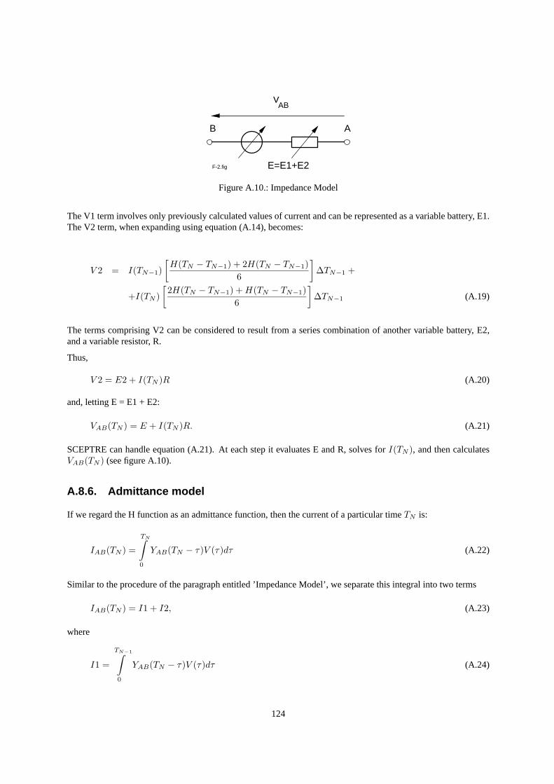
F-2.fig
B A
ABV
E=E1+E2
Figure A.10.: Impedance Model
The V1 term involves only previously calculated values of current and can be represented as a variable battery, E1.The V2 term, when expanding using equation (A.14), becomes:
V 2 = I(TN−1)[H(TN − TN−1) + 2H(TN − TN−1)
6
]∆TN−1 +
+I(TN )[
2H(TN − TN−1) +H(TN − TN−1)6
]∆TN−1 (A.19)
The terms comprising V2 can be considered to result from a series combination of another variable battery, E2,and a variable resistor, R.
Thus,
V 2 = E2 + I(TN )R (A.20)
and, letting E = E1 + E2:
VAB(TN ) = E + I(TN )R. (A.21)
SCEPTRE can handle equation (A.21). At each step it evaluates E and R, solves forI(TN ), and then calculatesVAB(TN ) (see figure A.10).
A.8.6. Admittance model
If we regard the H function as an admittance function, then the current of a particular timeTN is:
IAB(TN ) =
TN∫0
YAB(TN − τ)V (τ)dτ (A.22)
Similar to the procedure of the paragraph entitled ’Impedance Model’, we separate this integral into two terms
IAB(TN ) = I1 + I2, (A.23)
where
I1 =
TN−1∫0
YAB(TN − τ)V (τ)dτ (A.24)
124
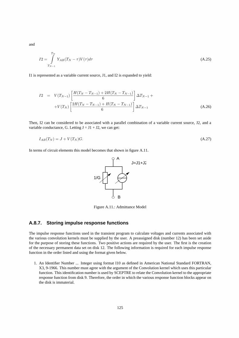
and
I2 =
TN∫TN−1
YAB(TN − τ)V (τ)dτ (A.25)
I1 is represented as a variable current source, J1, and I2 is expanded to yield:
I2 = V (TN−1)[H(TN − TN−1) + 2H(TN − TN−1)
6
]∆TN−1 +
+V (TN )[
2H(TN − TN−1) +H(TN − TN−1)6
]∆TN−1 (A.26)
Then, I2 can be considered to be associated with a parallel combination of a variable current source, J2, and avariable conductance, G. Letting J = J1 + J2, we can get:
IAB(TN ) = J + V (TN )G. (A.27)
In terms of circuit elements this model becomes that shown in figure A.11.
B
A
1/G
J=J1+J2
Figure A.11.: Admittance Model
A.8.7. Storing impulse response functions
The impulse response functions used in the transient program to calculate voltages and currents associated withthe various convolution kernels must be supplied by the user. A preassigned disk (number 12) has been set asidefor the purpose of storing these functions. Two positive actions are required by the user. The first is the creationof the necessary permanent data set on disk 12. The following information is required for each impulse responsefunction in the order listed and using the format given below.
1. An Identifier Number ... Integer using format I10 as defined in American National Standard FORTRAN,X3, 9-1966. This number must agree with the argument of the Convolution kernel which uses this particularfunction. This identification number is used by SCEPTRE to relate the Convolution kernel to the appropriateresponse function from disk 9. Therefore, the order in which the various response function blocks appear onthe disk is immaterial.
125
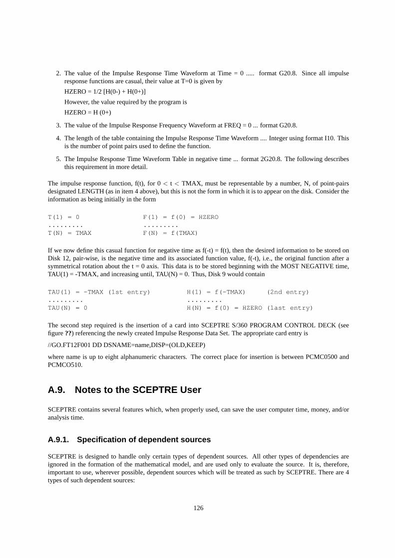
2. The value of the Impulse Response Time Waveform at Time = 0 ..... format G20.8. Since all impulseresponse functions are casual, their value at T=0 is given by
HZERO = 1/2 [H(0-) + H(0+)]
However, the value required by the program is
HZERO = H (0+)
3. The value of the Impulse Response Frequency Waveform at FREQ = 0 ... format G20.8.
4. The length of the table containing the Impulse Response Time Waveform .... Integer using format I10. Thisis the number of point pairs used to define the function.
5. The Impulse Response Time Waveform Table in negative time ... format 2G20.8. The following describesthis requirement in more detail.
The impulse response function, f(t), for 0< t < TMAX, must be representable by a number, N, of point-pairsdesignated LENGTH (as in item 4 above), but this is not the form in which it is to appear on the disk. Consider theinformation as being initially in the form
T(1) = 0 F(1) = f(0) = HZERO......... .........T(N) = TMAX F(N) = f(TMAX)
If we now define this casual function for negative time as f(-t) = f(t), then the desired information to be stored onDisk 12, pair-wise, is the negative time and its associated function value, f(-t), i.e., the original function after asymmetrical rotation about the t = 0 axis. This data is to be stored beginning with the MOST NEGATIVE time,TAU(1) = -TMAX, and increasing until, TAU(N) = 0. Thus, Disk 9 would contain
TAU(1) = -TMAX (1st entry) H(1) = f(-TMAX) (2nd entry)......... .........TAU(N) = 0 H(N) = f(0) = HZERO (last entry)
The second step required is the insertion of a card into SCEPTRE S/360 PROGRAM CONTROL DECK (seefigure??) referencing the newly created Impulse Response Data Set. The appropriate card entry is
//GO.FT12F001 DD DSNAME=name,DISP=(OLD,KEEP)
where name is up to eight alphanumeric characters. The correct place for insertion is between PCMC0500 andPCMCO510.
A.9. Notes to the SCEPTRE User
SCEPTRE contains several features which, when properly used, can save the user computer time, money, and/oranalysis time.
A.9.1. Specification of dependent sources
SCEPTRE is designed to handle only certain types of dependent sources. All other types of dependencies areignored in the formation of the mathematical model, and are used only to evaluate the source. It is, therefore,important to use, wherever possible, dependent sources which will be treated as such by SCEPTRE. There are 4types of such dependent sources:
126

1. Resistor-dependent voltage sources:
Exx, node 1 - node 2 = constant *VRyy
2. Resistor-dependent current sources:
Jxx, node 1 - node 2 = constant *IRyy
3. Diodes:
Jxx, node 1 - node 2 =
• DIODE Q (a,b)
• or
DIODE EQUATION (a,b)
• or
DIODE T xy
• or
DIODE TABLE xy
4. Diode dependent current sources:
Jxx, node 1 - node 2 = variable *Jyy
where Jyy is a diode current source
Such sources must be specified exactly as shown. Variations in forms such as Exx = X1 (3.*VRyy), will not beidentified as type 1 sources by SCEPTRE, and may lead to a computational delay.
Correct specification of dependent sources will, in general, produce a larger step size in transient runs, and faster,more reliable convergence in initial condition runs, leading to a decrease in running time in both cases.
This is particularly important in AC calculations. Only sources 1 recognizable as AC sources or one of the fourdependent sources described here are used in AC calculations. All others are considered DC sources and set tozero.
A.9.2. Proper use of dependent sources
in many cases, it is to the user’s advantage to force his dependent sources into one of the four types recognizedby SCEPTRE (see A.9.1). Thus, a circuit containing a source dependent on capacitor voltage, specified in astraightforward manner as
E1, N1-N2 = X1 (3.*VC1)C1, NA-NB =....
could be rewritten with a large resistor in parallel with C1, allowing the source to become a resistor-dependentsource
127
E1, N1-N2 = 3.*VR1CL, NA-NB =....R1, NA-NB = large number
This technique may not be helpful if it requires a significant increase in the number of circuit elements.
Similarly, a voltage source depending on the current through a fixed resistor
E1, N1-N2 = X1 (3.*IR1)R1, NA-NB = 2.
should be specified in the following electrically equivalent form which will be recognized by SCEPTRE as a type1 source
E1, N1-N2 = 1.5*VR1R1, NA-NB = 2.
A.9.3. Avoiding computational delay
A computational delay occurs when the specification of an element depends on a circuit variable which SCEPTREhas not yet computed at this time step. The value at the previous step is used. This may force a smaller step size thanwould otherwise be required. There are two techniques for avoiding this in certain circumstances. One is to specifythe element as one of SCEPTRE’s special dependent sources (see A.9.1 and A.9.2). When this cannot be done, theuser should rerun Phase I only, specifying WRITE SIMUL8 DATA under RUN CONTROLS. An examination ofthe SIMUL8 program generated may indicate a possible change of variables to avoid the computational delay. Forexample, if the specification
L2, node 1 - node 2 = X1 (P1*IR2)
produces a computational delay, and examination of the SIMUL8 program shows that P1 and VR2 have beencalculated while IR2 has not, L2 should be respecified as
L2, node 1 - node 2 = X1 (P1*VR2/R2)
A.9.4. Overcoming restrictions in initial conditions runs
The restrictions on initial conditions circuits described in the SCEPTRE manual [2, p. 40] apply only to theNewton-Raphson method of initial conditions solution. They do not apply to the alternate initial conditions solutionusing implicit integration of the transient equations. It is therefore advised that initial conditions for a circuit befound using SCEPTRE’s transient model, instead. This is done by inserting in the RUN CONTROLS section thecard RUN IC VIA IMPLICIT.
A.9.5. Error checking in IC VIA IMPLICIT
Theoretically, a circuit containing capacitor-current source cut-sets and/or inductor-voltage source tie-sets (i.e.,loops) has no DC solution. This condition is detected by the default (Newton-Raphson) SCEPTRE initial conditionroutines, an error message is printed, and execution stops. This is not the case if the user has specified RUN ICVIA IMPLICIT. SCEPTRE will attempt to solve the problem, resulting in a long, and useless run. It is, therefore,advisable to check the circuit before using IC VIA IMPLICIT.
128

A.9.6. Element sort
The state variables chosen by SCEPTRE are partially dependent on the ordering of the input under ELEMENTS.It is sometimes helpful in cases where SCEPTRE chooses an inconveniently small step size for a transient run toresubmit the run with a different ordering of elements. This will result in a new choice of state variables, whichmay have larger time constants. To get the effect of this reordering, the card
NO ELEMENT SORT
should be included under RUN CONTROLS.
Since this technique requires some experimentation, it is wise to limit the duration of the run (COMPUTER TIMELIMIT = ...) and try several different element orderings. The best one can then be used for the complete run.
A.9.7. Output reduction
SCEPTRE produces printed output of each variable which it plots. This often results in unnecessarily large volumesof output and high charges for printing. If the user requires only plotted output, he should specify MAXIMUMPRINT POINTS = 1 in the RUN CONTROLS section. To allow a subsequent list of the out variables, the runshould be set up to permit a RE-OUTPUT run.
A.9.8. Some frequent errors
The user should note that output controls must be under the RUN CONTROLS heading, rather than the OUTPUTSheading.
Thus, PLOT INTERVAL = .... and PRINT INTERVAL = ..... are both considered RUN CONTROLS and shouldappear in that section of input.
A.9.9. DC coupling capacitor in certain AC runs
The user is encouraged to insert a DC coupling capacitor in series with all AC voltage sources for AC problemswhich require initial condition solution. During the IC solution, the AC source is set to zero, forming a shortand allowing current through the source. The capacitor prevents any current from flowing through that branch,resulting in the correct IC solution.
Analogously, an inductor should be connected in parallel with an AC current source. This forces a short across thecurrent source, which has been set to zero (open circuit), for the IC run. This prevents any voltage from appearingacross the source.
In both cases, the value of the element should be large enough so it does not load the source driving the AC run.That is, the capacitor should appear as a short circuit and the inductor should appear as an open circuit at the lowestanalysis frequency.
A.9.10. Convolution input
The input function h for convolution must specify h(0). (See section A.8.7 page 125). In cases where there is noenergy in the total circuit at t = 0, any value may be given for h(0) since it has no effect on circuit behavior.
129
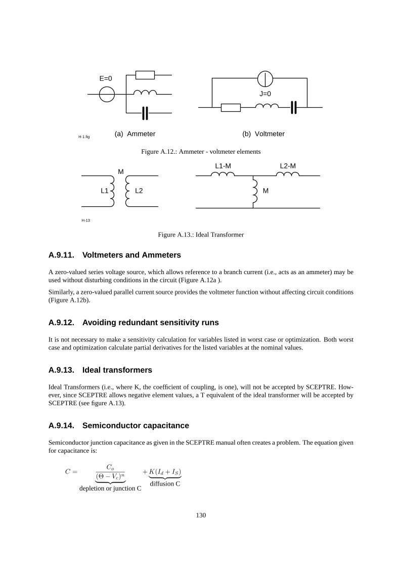
E=0
(b) Voltmeter
J=0
H-1.fig (a) Ammeter
Figure A.12.: Ammeter - voltmeter elements
H-13
L2-M
M
L1-MM
L1 L2
Figure A.13.: Ideal Transformer
A.9.11. Voltmeters and Ammeters
A zero-valued series voltage source, which allows reference to a branch current (i.e., acts as an ammeter) may beused without disturbing conditions in the circuit (Figure A.12a ).
Similarly, a zero-valued parallel current source provides the voltmeter function without affecting circuit conditions(Figure A.12b).
A.9.12. Avoiding redundant sensitivity runs
It is not necessary to make a sensitivity calculation for variables listed in worst case or optimization. Both worstcase and optimization calculate partial derivatives for the listed variables at the nominal values.
A.9.13. Ideal transformers
Ideal Transformers (i.e., where K, the coefficient of coupling, is one), will not be accepted by SCEPTRE. How-ever, since SCEPTRE allows negative element values, a T equivalent of the ideal transformer will be accepted bySCEPTRE (see figure A.13).
A.9.14. Semiconductor capacitance
Semiconductor junction capacitance as given in the SCEPTRE manual often creates a problem. The equation givenfor capacitance is:
C =Co
(Θ− Vc)n︸ ︷︷ ︸depletion or junction C
+K(Id + IS)︸ ︷︷ ︸diffusion C
130

When the junction is forward biased the denominator of the first term in the equation becomes negative. Since thevalue of n lies between 1/2 and 1/3, the first term becomes complex. However, according to the basic physics ofsemiconductors, the first term of the equation is valid only if the junction is reverse biased. To avoid this problem,use instead two capacitors in parallel.
Cj , which models the first term in the equation can be given either as a constant or as a table, which will be a betterrepresentation of the semiconductor physics. The second capacitor,CD = K(ID + IS), should be given by anequivalent equation to avoid unnecessary computation:
CD = K[IS(eΘVc − 1) + IS
]= KISe
ΘVc
A.9.15. Rerun
Under RERUN DESCRIPTION, it is not possible to change a constant to a table or equation. This can be done,however, by specifying the constant as a table or equation in the master run, which can be changed to a differenttable or equation in reruns.
131

Bibliography
[1] D. Becker.Extended SCEPTRE Vol. 1, User’s Manual.AFWL-TR-73-752 (NTIS3: ADA 009594)
[2] D. Becker.Extended SCEPTRE Vol. 2, Mathematical Formulation.AFWL-TR-73-75 (NTIS: ADA 009595)
[3] J.C. Bowers, S.R. Sedore.SCEPTRE: A Computer Program for Circuit and System Analysis.Englewood Cliffs, N.J., Prentice-Hall, Inc., 1971
[4] R. W. Jensen, M. D. Lieberman.IBM Electronic Circuit Analysis Program Techniques and Applications.Englewood Cliffs, N.J., Prentice-Hall, Inc., 1968
[5] Advanced Statistical Analysis Program (ASTAP) General Information Manual.IBM GH20-1271-0
[6] R. W. Jensen, L. P. McNamee.Handbook of Circuit Analysis Languages and Techniques.Englewood Cliffs, N.J., Prentice-Hall, Inc., 1976
[7] James C. Bowers, et al.A survey of Computer-Aided-Design & Analysis ProgramsAFAPL-TR-76-33 (NTIS: AD-A 026567)
[8] Soo Young Shin.A Survey of Computer-Aided Electronic Circuit Analysis ProgramsNTIS: AD-A 009185
[9] H. Spiro. Simulation integrierter Schaltungen durch universelle Rechnerprogramme: Verfahren und Praxisder rechnergestützten Simulation nichtlinearer Schaltungen.Verlag Oldenbourg, München , 1985
[10] J. I. Lubell.Transmission Line Modeling for Use with Circuit/System Analysis Programs.AFWL-TR-73-128 (NTIS: AD 913-800)
[11] P. Krehl, W.-R. Novender.A Graphical and Analytical Method to Determine the Transient Response for anIdeal Transmission Line, Loaded by a Time-Varying Impedance.IEEE Transactions on Plasma Science, Vol. PS-13, No. 2, April 1985
[12] C. B. Frye, Jr., M. J. Apfelbaum.Mixed Domain Transient Analysis of Large Non-Linear Networks.Tenth Annual Allerton Conference on Circuit and System Theory, October 1972
[13] W. Kaplan.Ordinary Differential Equations.Addison Wesley, Reading, Mass., 1958, Section 10-2, pp. 400–401.
[14] eb.da, Section 10-4,“Heun’s Method”, pp. 402–403
[15] K. G. Ashar, H. N. Ghosh, A. W. Aldridge, L. J. Patterson.Transient Analysis and Device Characterizationof ACP Circuits.IBM Journal of Research and Development, Vol. 7, p. 218, 1963
2Air Force Weapons Laboratory, Kirtland, AFB, NM 87117, USA3National Technical Information Service, Springfield, VA 22151, USA
132

[16] P. E. Chase.Stability Properties of Predictor-Corrector Methods for Ordinary Differential Equations.Journal A.C.M 9, October 1962, pp. 457–468
[17] R. J. Kuhler.Application of Generator Analysis Methods.AFAPL-TR-77-31 (NTIS: AD A042071)
[18] Wm. C. Davidon.Variable Metric Method for Minimization.AEC Research and Development Report ANL-5990 (REV) 1959
[19] M. J. Box.A Comparison of Several Current Optimization Methods, and the Use of Transformation in Con-strained Problems.The Computer Journal 9, pp. 67-77, 1966
[20] M. J. Box, D. Davies, W. G. Swann.Non-Linear Optimization Techniques.Imperial Chemical Industries, Ltd. Monograph No. 5, 1969
[21] Variable Metric Minimization.SHARE Routine No. 1117, AN Z013, A3. SHARE Inc., Suite 750, 25 Broadway New York, NY 10004
[22] J. C. Bowers, J. E. O’Reilly, G. A. Shaw.SUPER-SCEPTRE – A Program for the Analysis of Electrical,Mechanical, Digital and Control Systems.University of South Florida, Tampa, Florida 33620, May 1975(NTIS: AD A011348)
[23] W. A. Cordwell.Transistor and Diode Model Handbook.AFWL-TR-69-44 (NTIS: AD 862556)
[24] Y. C. Liang, V. J. Gosbell.A Versatile Switch Model for Power Electronics SPICE2 Simulations.IEEE Transactions on Industrial Electronics, vol. 36, no. 1, February 1989, p. 86
[25] Lawrence J. Giacoletto.Simple SCR and TRIAC PSPICE Computer Models.IEEE Transactions on Industrial Electronics, vol. 36, no. 3, August 1989, p. 451
[26] F. Javier Gracia, Fernando Arizti, F. Javier Aranceta.A Nonideal Macromodel of Thyristor for TransientAnalysis in Power Electronic Systems.IEEE Transactions on Industrial Electronics, vol. 37, no. 6, December 1990, p. 514
[27] Vineeta Agrawal, Anant K. Agarwal, Krishna Kant.A Study of Single-Phase to Three-Phase Cycloconverterusing PSPICE.IEEE Transactions on Industrial Electronics, vol. 39, no. 2, April 1992, p. 141
[28] H. A. Nienhaus, J. C. Bowers, M. S Ziemacki.A Computer Model for a High Power SCR.AFAPL-TR-75-1064 (NTIS: ADA 022375)
4Air Force Aero Propulsion Laboratory
133