extending the notion of riemann integral to lebesgue
TRANSCRIPT

1
EXTENDING THE NOTION OF RIEMANN INTEGRAL TO LEBESGUE INTEGRAL ON
2
R AND APPLICATIONS IN TIME SERIES ANALYSIS.
BY
FRANCIS NDONGA CHEGE
A project submitted to the school of mathematics in partial
fulfillment for a degree of master of science in pure mathematics
to School Of Mathematics. University Of Nairobi
2rd September 2016

2
CONTENTS
Declaration (i)
Acknowledgement (ii)
Dedication (iii)
Abstract (iv)
CHAPTER 1 INTRODUCTION
1.1 General Introduction 9
1.2 Problem statement 9
1.3 Objectives 9
1.4 Significance Of Study 9
CHAPTER 2. LITERATURE REVIEW 10-11
CHAPTER 3. RIEMANN INTEGRATION
3.1 Partition 12
3.2 Bounded Variation 12-14
3.3 Total Variation 16-17
3.4 Riemann Integration 19-23
3.5 Calculus Theorems Allied to Riemann Integrals
3.6Indefinate and definite Integrals 25
3.7Fundamentals theorems of integral calculus 26
3.8Integration by Parts 27
3.9Cauchy-Schwartz Inequality 27-28
3.10 Mean Value Theorem(M.V.T) of Integral Calculus 28
CHAPTER4 RIEMANN STIELTJES INTEGRATION
4.1 Riemann Stieltjes Integration 29-33
4.2 Step Function 34-35
4.3 Change Of Variable Theorem 36
4.4 Integration Of Vector Valued Functions 37-38

3
4.5 Rectifiable Curves 39-41
CHAPTER 5. LEBESGUE INTEGRATION
5.1 Introduction 42
5.2 The lebesgue measure 43-48
5.3 The lebesgue integral for Non-negative simple functions 49-50
5.5 The integral of a non-negative measurable functions 51
5.6 Monotone Convergence Theorem (M.C.T) 52-55
5.7 Fatou’s Lemma 56-57
5.8 Lebesgue Dominated Convergence Theorem (L.D.C.T) 57-59
CHAPTER6. COMPARISION OF LEBESGUE AND RIEMANN INTEGRABLE FUNCTIONS.
6.1 Bounded Functions 60-62
6.2 Lebesgue and Riemann Integrals for Unbounded functions 63-64
6.3 Libesgue and Riemann integration and the connection
of a function and its anti-derivative 65-66
6.4 Functions of Class L2 67-69
6.5 Integration of complex(analytic) expressions and Lp-spaces 70-73
CHAPTER 7 APPLICATIONS TIME SERIES ANALYSIS
7.1 Variation And Linear Regression Model 74-75
7.2 Fourier Series 77-79
7.3 Time Series And Smoothing Process 80-82
7.4 Auto Correlation 83-84
7.5 Wavelet Analysis 85-89
7.6 Spectral Analysis 90-92
Conclusion 93
Recommendations 94
Bibliography 95

4
DECLARATION
Declaration by the student
I the undersigned ,declare that this project is the original work
and has not been used as a basis for any degree in any other University
FRANCIS NDONGA CHEGE
REG.NO . I56/76350/2014
……………. …………….
This Project has been submitted with my approval as the university supervisor
SUPERVISOR
……………… ……………..
Signature Date

5
ACKNOWLEGEMENTS
Glory and Honor to the Almighty God to the highest .For giving me strength to
Move on even when I am in the weakest spirit and moments.
I am very grateful to my supervisors Dr.J.N.Muriuki and Prof J. Khalaghai for
their relentless support, direction and clarity while researching this project.
I would also not forget to reminisce the crucial background support from Msc. pure
Math’s lecturer’s, colleagues, librarians, and authors .Finally much appreciation to
University of Nairobi for the chance to undertake the postgraduate program.

6
DEDICATION
To my young , teenage and Adult friends, the selfless in doing together and sharing ,
that we extend often is a milestone .The non dangerous adventures ,cheerful spirit ,
conventional with understanding of the goals . The future is us, and we direct virtues ,
talents and hard work. You are uncountable and wish to be anonymous ,but request to
Thank you all ,for this far. And great things in store are endless. We can do it
again certainly.

7
ABSTRACT
This research work is intended for Senior undergraduate course in analysis ,’The 3rd and 4th
year B.ed and B.sc mathematics options’ and first year student mastering in mathematics. The
project covers topics in calculus ,real analysis, measure theory and applications in time series.
The beginning chapters lay the setting to Riemann integration in contrast with other earlier
existing theories such us mid-ordinate rule and Trapezium method. Riemann defines partition of
independent ordinate and take variation of the dependent ordinate then proceed to take the
minimum and maximum sum of all the partitions possible and the integral is taken if the two
Riemann sum are equal. Some examples of integration are also provided. The theory of Riemann
stieltjes is an extension of Riemann theory that covers ;vector- valued functions and discontinuous
functions such unit step functions and signum functions. It’s bridge the gap of continuity and
discontinuity by use of convergence of series and also extend the real line to n
R spaces. The
final and most notable extension is the lebesgue integration. The construction of the lebesgue
measure is done using countable base, whose members are open interval then the idea of
measurable functions is extensively discussed ,before it’s use in definition of measurable integral
is important ,the we proceed to define monotone convergence theorems and lebesgue dominated
convergence theorems. Finally the comparison of the two integration theories ‘Riemann and
lebesgue’ is done by citing a number of similarity and loopholes in evaluation of integral in areas
such as ;Bounded and Un bounded functions ,Complex and PL -spaces and recovery of derivative
functions. Finally application of the Fourier Series integrals in Time-Series Analysis is done by
by smoothing time plot by regression and other methods which allow finding of auto correlation ,
wavelet and spectrum analysis.

8
CHAPTER ONE
1.0 INTRODUCTION
1.1 General Introduction
Integration means bringing parts together ,it is the process that is inverse to differentiation.
Thus the definite integration, ”Let f be defined on the interval [a,b],the definite integral of f
Is given by ( ) lim ( ) ,
b
in
a
f x dx f x x→∞
= ∆∑∫ ,provided the limits exists, where ( )b a
xn
−∆ = and i
x
is any value of x in thi interval. This definite integral is a number ( example of Riemann sum)
The fundamental Theorem of calculus ,’let f be continuous on the interval[a,b] and let F be
any ant derivative of f .Then ( ) ( ) ( ) ( ) |
b
b
a
a
f x dx F b F a F x= − =∫ which shows connection of
between ant derivatives and definite integrals.Other important theorems allied to Riemann
includes the Archimedes ( 287 213 .B C− ) ,First Principles and mean value theorem.
Riemann integral became inadequate and could not give solutions in discontinuity as well as Functions with increasing number of limits. Thus extensions such as Riemann Stieljes and Lebesgue integration theories allows us to integrate a much larger class of functions such as step-wise functions(discontinuous functions)and also many limits operations can be handled with a lot of ease.

9
1.2 PROBLEM STATEMENT
Many research studies has been done on the integration techniques ,but very few of
their feedback narrow back to its development from reasonably well-behaved functions on
sub-intervals of real line. As well as developed theories of integrations that can be applied to much
large classes of functions whose domains are more or less arbitrary set ,including subsets of 2
R
This research aim to put across different ways of approximating areas of the regions, the
Riemann theory and extensions by Stieltjes and Lebesgue and also its applications in time
series analysis
1.3 OBJECTIVES
The overall objectives is to survey the formulation (or derivation) of both Riemann integral
and Lebesgue integral and make a brief comparison between theories.
1.4 Specific Objectives
1 .Investigate the fundamental concepts of Riemann and Riemann-Stieltjes theory of integration.
2. Construction of the lebesgue measure and integration and some of the main theorems of the
theory.
3.Make a brief comparison stating where possible advantages of Lebesgue integral theory over
the Riemann integral theory.
4.Exhibit examples to show applications in Time Series Analysis.
1.5 SIGNIFICANCE OF STUDY
Lebesgue integration have wide range of applications in statistics of expectations, Solutions to
time series analysis and research methods. Furthermore integration and differentiation is very vital
in applied and Engineering mathematics. It also occupy a central place in analysis , in the study of
( L2-Spaces and L
p-spaces).
10
CHAPTER 2
2.0 LITERATURE REVIEW
2.1 Motivation
Three Cambridge University Dons of mid 20th− Century in their three books,
‘Cambridge Mathematics; Part I ,Part II ,and Part III ,classified the subject into
(i)Mathematics for pre-university/undergraduate mathematics
(ii)Applied mathematics of specialized courses and
(iii)Mathematics Analysis
Riemann and Lebesgue Theories Of Integration are some of earlier stage of analysis and extending the
study of real line to n
R spaces just make it much involved .Furthermore application of orthogonal integral to
time series analysis is crucial in Biostatistics ,geophysics and financial fields
2.2 Background Information.
The concepts of integration dates backs to ( (287 213 . )B C− ) where Archimedes and his
contemporaries would apply the first principles to find area of planes figures even before the method
of differentiation was discovered. Otherwise, the concepts of integration as a technique that both acts
as a an inverse to the operation of differentiation and also compute area under curves ,goes back to the
origin of calculus and the work of Isaac Newton (1643 1727)− and Leibnitz (1646 1716)−
It was Leibnitz who introduced the ∫ …dx notation. The first rigorous attempt to
understand integration as a limiting operation within the spirit of analysis was due to
Bernard Riemann (1826 1866).− The approach of Riemann that is usually taught was however
developed by Jean-Gaston Dar boux (1842 1917)− .at the time it was developed this theory seemed
to be all that was needed but as the 19th century drew
closer, some problem appeared.
(i)One of the main tasks of integration is to recover a function f from it’s derivative 'f .
but some functions were discovered for which 'f was bounded but not Riemann integrable.

11
(ii)Suppose ( )n
f is a sequence of functions converging point wise to f . The Riemann integral
could not be used to find conditions for which ( ) lim ( )nn
f x dx f x dx→∞
=∫ ∫
(iii)Riemann integration was limited to computing integrals over 2
R with respect to Lebesgue measure,
although it is not yet apparent ,the emerging theory of probability would require the calculation of
expectations of random variables ; ( ) ( ) ( )x E X x w dp wΩ
= ∫ .The Lebesgue’s technique allows us to
investigate ( ) ( )s
f x dm x∫
where ;f S R→ is a ‘suitable’ measurable function defined on a measure
space ( , , )S M∑ , If we take M to be the Lebesgue measure on ( , ( ))R B R . we recover
the familiar integral ( )R
f x dx∫ but we will now be able to integrate many more functions
(at least in principles)than Riemann and Darboux. If we take X to be a random variable on a
probability space, we get it’s expectation ( )E x .
2.3 COMPARISON
Many authors such as have compared the two theories Riemann and Libesgue inform
of integral theorem, but much of comparisons tools will depend on the calculus
reader/student in identifying the key areas, applications and the successes or failure of each
method. This article cite five such areas namely; Integration of discontinuous functions, Relation
of differentiation and integration, complex functions and 2L space− s.
2.4 APPLICATION
There are wide range of stationary time series models methods for estimation of autocorrelation
and spectrum as well as methods for multivariate stationary series, and those that forecasting
future values . Authors who have written materials in this field includes
Priestly .M,’ Spectral Analysis and Time Series’. Hannan. E.J,’ Time Series Analysis.’ etc..

12
CHAPTER THREE
RIEMANN INTEGRATION
3.1.0 (Partition)
3.1.1 Definition; Let [a, b] be a compact interval. Then the set of points 1, ,..........o np x x x=
satisfying the inequality 0 1 2..........n
a x x x x b= < < < = is called a partition of [ , ]a b
0 1 1.............
| | | |a x n nx x x b= − =
3.1.2 Consequences
(a) 1k k kx x x −∆ = − such that
1
n
k
k
x b a=
∆ = −∑
(b) collection of all possible partition on [ , ]a b is denoted by ( , ) [ , ]Q a b P Q a b⇒ ∈
I .e P is a partition of [ , ]a b
3.2.0 Bounded Variation ( Bounded Variation )
3.2.1 Definition ; Let f be a function on [ , ]a b with 1
( ) ( ) ( )k k k
f x f x f x −∆ = − , if there exist a
number M such that M>0 and 1| ( ) ( ) |k kf x f x M−− ≤∑ [ , ]p Q a b∀ ∈ .
Then the function f is said to be bounded variation on [ , ]a b and is denoted by . [ , ]f BV a b∈ .
Y
( )k
f xλ =
1( )
kf xµ −=
|a
|b
X

13
3.2.2 Theorem
If f is monotonic on [ , ]a b then . [ , ]f BV a b∈
Proof
A monotonic f is either an increasing ( )↑ or decreasing ( )↓ function on
an interval [ , ]a b . (i)When f is increasing ( )↑ on [ , ]a b
Then for every partition of [ , ]a b we have 1( ) ( ) 0
k kf f x f x −∆ = − ≥
Hence 1 1
1 1 1
( ) ( ) ( ) ( )k
n n n
k k k
i i i
f x f x f x f x− −
= = =
− = −∑ ∑ ∑
( ) ( )f b f a= −
Putting ( ) ( )f b f a M− = , hence for all possible partitions ,
. [ , ]f BV a b∈ since 1
| |n
k
k
fx M=
∆ ≤∑
(ii)If f is decreasing ( )↓ on [ , ]a b
Then for every partition of [ , ]a b
We have 1
( ) ( ) ( ) 0k k k
f x f x f x−∆ = − ≥
Hence 1 1
1 1 1
| ( ) ( ) | ( ) ( )n n n
k k k k
i i i
f x f x f x f x− −= = =
− = −∑ ∑ ∑
( ) ( )f b f a= −
Putting ( ) ( )f b f a M− = implies that 1
| |n
k
k
fx M=
∆ ≤∑
Hence for all partitions on [ , ], . [ , ]a b f BV a b∈

14
3.2.3 Def ( ε δ− ,definition of continuity)
A function ( )f x is continuous at a point a if for every number 0ε > their exist 0δ >
Such that | | | ( ) ( ) |x a f x f aδ ε− < ⇒ − <
( )f b _ ( )f x
( )f a _
|a
δ |x
X
3.2.4 Example
The function 2 5
( )4
xf x
x
−=
− is continuous at 5x = since
2
5
5lim
4x
x
x→
−−
has a value(exist).
On the contrary ( )f x is not continuous at 4x = , because its limit has no value.
Proof
f(x) f(x)
ε
f(a) δ
a x
In this case 5a = , 2 5
( )4
xf x
x
−=
−
choose any 0ε > and fix it such that | ( ) ( ) |f x f a ε− <
i.e 2 5
| 20 |4
x
xε
−− <
− or
2 5 20 80| |
4
x x
xε
− − +<
−
=2 20 75
| |4
x x
xε
− +<
−=
( 5)( 15)|
4
x x
xε
− −<
−

15
= 15
| ( 5) || |4
xx
xε
−− <
−
= 4
| 5 | | |15
xx
xε
−− <
−
1
10(for x close to 5)
i.e | 5 |10
xε
δ− < = Thus 0δ > and | 5 |x δ− <
whenever | 5 |x δ− < | ( ) (5) |f x f ε⇒ − <
3.2,5 . Theorem; Let f be continuous in [ , ]a b , if the derivative 'f of the function f exist
and is bounded on [a, b] such that for ( , ),x a b∀ ∈ then f is of bounded variation.
Recall mean value theorem 1
1
( ) ( )'( ) k k
k
k k
f x f xf t
x x
−
−
−=
− and 1( ) ( ) ( )
k k kf x f x f x −∆ = −
by mean value theorem 1( ) '( )( )
k k k kf x f x x x −∆ = − '( )
k kf t x= ∆ where 1k k k
x t x− ≤ ≤
And hence | | | '( ) |k k
f f t x∆ = ∆∑ ∑ ( )A b a≤ − Putting ( )A b a M− = ,
we have | |k
f M∆ ≤∑ i. e f is a bounded variation.

16
3.3.0 Total Variation
3.3.1 Def ;Let . [ , ]f BV a b∈ and let 1| ( ) ( ) |k kSp f x f x −= −∑ corresponding to the partition
0 1 2, , .......... np x x x x= ( )k
f x
1)( kf x −
0 1...... ...
| . . |k na x x x b x= =
Let [ , ]Q a b be the set of all partition of [ , ]a b , the number
( , ) ; ( , )f p
V a b Sup s p Q a b= ∈
1| ( ) ( ) |p k kSup s f x f x −= = −∑ | ( , )P Q a b∈ is called the total variation of f on [ , ]a b .
3.3.2 Theorem
Let . ( , )f BV a b∈ and let a c b< < then . [ , ]f BV a c∈ and . [ , ]f BV c b∈ furthermore
[ , ] [ , ] [ , ]f f fV a b V a c V c b= +
Proof
(I)Showing ( , ) ( , ) ( , )f f fV a c V c b V a b+ ≤
Let 1p and 2
p be any arbitrary partitions of [ , ]a c and [ , ]c b respectively. Then 20 1p p p= ∪ is a
partition of [ , ]a b .Let 1| ( ) ( ) |i k kSp f x f x −= −∑ , corresponds to the partitions i
p (for arbitrary
appropriate interval) then 1 2 0 1( , )f
p p Sp V a b Sp+ = ≤ ⇒∑ ∑ and 2Sp are bounded above by
( , )fV a b ,Which implies that 1 1| ( ) ( ) | ( , )k k f
Sp f x f x V a b−= − ≤∑ and
2 1| ( ) ( ) | ( , )k k f
Sp f x f x V a b−= − ≤∑ hence f is of bounded on [ , ]a c and [ , ]c b and from above
we have ( , ) ( , ) ( , )f f f
V a c V c b V a b+ ≤.

17
(II)To show ( , ) ( , ) ( , )f f f
V a b V a c V c b≤ +
Let 0 0 1, ,..........n
p x x x= be partition on [ , ]a b and let 'P P c= ∪ obtained by adjoining
a point c in 0p .If 1( , )k k
c x x+∈ then 1 1| ( ) ( ) | | ( ) ( ) | | ( ) ( ) |k k k k
f x x f c f x f c f x− −− ≤ − + + so
that 0 'Sp Sp≤ .The points P which belongs to [ , ]a c and the points of P which belongs to [ , ]c b
determines the partitions 1p and 2p hence 0 1 2'Sp Sp Sp Sp≤ = + I .e 0 1 2Sp Sp Sp≤ +
( , ) ( , )Vf a c Vf c b≤ + ( , ) ( , ) ( , )f f fV a b V a c V c b⇒ = +
3.3.3 Theorem
Let [ , ]f BV a b∈ and consider the function F defined
in [a, b] by ( , ); ...
( )0; .....
fv a x if a x b
f xif x a
< <=
= then F(↑) and F-f(↑)
Proof
For a x y b< < ≤ we have ( , ) ( , ) ( , )f f fV a b V a x V x y= + ……….(i)
so that ( ) ( ) ( , )f
F y F x V x y= + ( , ) ( ) ( )f
V x y F y F x⇒ = −
( ) ( ) 0F y F x⇒ − ≥
( ) ( )F x F y⇒ ≤ but x y≤ F⇒ ↑ i. e non decreasing.
Also for a x y b≤ ≤ ≤ we have ( ) ( )F f y F f x− − − ( ) ( ) [ ( ) ( )]F y f y F x f x= − − −
[ ( ) ( )] [ ( ) ( )]F y F x f y f x= − − −
( , ) ( , ) [ ( ) ( )]f fV a y V a x f y f x= − − −
( , ) [ ( ) ( )] 0fV x y f y f x= − − ≥
( ) ( ) 0F f y F f x⇒ − − − =
( ) ( )F f x F f y⇒ − ≤ − but x y≤ I .e F f− ↑ hence non-decreasing

18
3.3.4 Theorem
A real valued function f defined on [a, b] is of bounded variation on [a, b]
if and only if f can be expressed as a difference of two non-decreasing
functions 1f and 2f i. e 1 2( ) ( ) ( )f x f x f x= − ,
with 1f and 2f non-decreasing on [a ,b].
Proof
Let . [ , ]f BV a b∈ then ( )f F F f= − − ,
Let F be defined as ( , );
( )0;........
fV a x a x b
F xx a
= < <=
=
Where both F and F f− have been shown to be
non-decreasing (by previous theorem)
Putting 1F f= and 1 2F f f− = then f can be expressed as a
difference of two non-decreasing functions.
Conversely
Let 1 2f f f= − when 1f and 2f are non-decreasing functions on [a, b]
1f and 2f are monotonic on [a, b]
Thus 1f and 2f are of bounded variation on [a, b].
Hence the difference 1 2f f− is of bounded variation on [a, b]
I .e 1 2f f f= − is of bounded variation.

19
3.4.0 RIEMANN INTEGRATION
3.4.1. Definition; Let f be continuous and bounded on [ , ]a b , divide [ , ]a b into n sub-divisions by points
0 1, ,.......n
x x x
Y
km k
M
0a x= 1x 2....x 1kx −
kb x=
X
Thus partition 0 1, ,........, nP x x x= such that 0 1 ..........n
a x x x b= < < < = .
Let the largest sub-interval have value 1k k kx x x −∆ = −
Let 1sup ( ) sup ( ); ( , )k k kM f x f x x x x−= = ∈ for 1k kx x x− < <
1inf( ) inf ( ); ( , )k k km x f x x x x−= = ∈ , for 1k kx x x− < < and for each partition
form the sum ( ) 1 1 0 2 2 1 1( ) ( )............. ( )p n n nS M x x M x x M x x −= − + − − =
1
n
k k
k
M x=
∆∑
Similarly ( ) 1 1 0 2 2 1 1( ) ( ) ...... ( )p n n ns m x x m x x m x x −= − + − + −
1
n
k k
k
m x=
= ∆∑
p
S and ( )p
s are called the upper and lower sum respectively ,by varying the partition we obtain
set of ( )pS and ( )ps ,Let ( )inf . .pU S g l b= = of the values of ( )pS ∀ possible partition. Let
( ) . .pL Sups l u b= = of all values of ( )ps ∀ possible partition. These values which always exist
are called upper and lower Riemann integrals of f over [a ,b] denoted by ( )
b
a
U f x dx= ∫ and
L = ( )
b
a
f x dx∫ If L U= i. e If the lower and upper integrals are equal then f is said be

20
Riemann-integrable over [ , ]a b and the common integral is denoted by ( )
b
a
I f x dx= ∫
(i)if U L≠ , f is not integrable over the interval [ , ]a b
(ii) the expression ( )I f x dx= ∫ is called the Riemann integral.
3.4.2 Theorem
Let f be continuous on [ , ]a b and a c b< < then ( ) ( ) ( )
b c b
a a c
f x dx f x dx f x dx= +∫ ∫ ∫
Proof
Let 1p and 2p be partition of [ , ]a c and [ , ]c b respectively and 1 2P p p= ∪
i.e P consists of at least one of the sets 1p and 2p ,where by ( )L SupS p=
clearly 1 2( ) ( ) ( )S P S p S p= + moreover ( ) ( )
b
a
S P L f x dx≤ ≤ ∫ , then given any 1p of [ , ]a b
and 2p of [ , ]a b 1 2( ) ( ) ( )
b
a
S p S p f x dx⇒ + ≤ ∫ 1 2( ) ( ) ( )...........( )
b
a
S p f x dx S p i⇒ ≤ −∫
For any part 2p of ( , )c b the right hand side of ( )i forms an upper bound of 1( )S p ,
1 2( ) ( ) ( )
b
a
SupS p f x dx S p⇒ ≤ −∫
1 2( ) ( ) ( ) ( )
c b
a a
SupS p f x dx f x dx S p⇒ ≤ ≤ −∫ ∫ i. e 2( ) ( ) ( )
c b
a a
f x dx f x dx S p≤ −∫ ∫
2( ) ( ) ( ) .....( )
b c
a a
S p f x dx f x dx ii⇒ ≤ −∫ ∫ ∀ partition 2p in [ , ]a b , the right hand side of ( )ii
forms an upper bound 1( ) ( ) ( )
b c
a a
SupS p f x dx f x dx⇒ ≤ −∫ ∫
2( ) ( ) ( ) ( )
b b c
c a a
SupS p f x dx f x dx f x dx⇒ ≤ ≤ −∫ ∫ ∫ Thus ( ) ( ) ( )
c b b
a c a
f x dx f x dx f x dx+ ≤∫ ∫ ∫ ……….*

21
To show the reverse inequality
Let P be any partition of [a, b] and Q be the partition obtained from P
by adjoining a point C in [a, b] P
a c b
1p 2p then ( ) ( )s p s Q≤
Let 1p be the part of [a,b] consisting those points of Q which lie on [a, c] and 2p be part
of [a, b] consisting of those points of Q which lie on [c, b] then
1 2( ) ( ) ( ) ( )s p s Q s p s p≤ = + ( ) ( )
c b
a c
f x dx f x dx≤ +∫ ∫
i.e ( ) ( ) ( )
c b
a c
s p f x dx f x dx≤ +∫ ∫ ,∀ possible partition P on [a, b]
( ) ( ) ( )
c b
a c
SupS p f x dx f x dx≤ +∫ ∫ ( ) ( ) ( ) ( )
b c b
a a c
SupS p f x dx f x dx f x dx≤ ≤ +∫ ∫ ∫Q
then ( ) ( ) ( ) ......**
b c b
a a c
f x dx f x dx f x dx≤ +∫ ∫ ∫
By * and ** equality is established i. e ( ) ( ) ( )
b c b
a a c
f x dx f x dx f x dx= +∫ ∫ ∫
3.4.3 Theorem
Let f be continuous on [ , ]a b with max ( )M f x= and min ( )m f x= on [ , ]a b
Then ( ) ( ) ( )m b a f x dx M b a− ≤ ≤ −∫
Proof
Let ( )p k kS M x= ∆∑ , ( )p k ks m x= ∆∑ since k K
m m M M≤ ≤ ≤ ,taking summation
22
from 1k = to n k k k K k km x m x M x M x∆ ≤ ∆ ≤ ∆ ≤ ∆∑ ∑ ∑ ∑ .For all possible partitions over
[ , ]a b thus we have ( ) ( ) ( ) ( )( ) inf ( )k p p k p pm x s S M x m b a Sups S M b a∆ ≤ ≤ ≤ ∆ ⇒ − ≤ ≤ ≤ −∑ ∑
But ( ) ( )( ) inf
b
p p
a
Sups f x dx S≤ ≤∫ hence ( ) ( ) ( )
b
a
m b a f x dx M b a− ≤ ≤ −∫
3.4.4 Properties of Riemann integral
1.If ( )f x c= where c is constant then ( ) ( )
b
a
f x dx c b a= −∫ .
2.Let f be continuous then ( ) ( ) ( )
b b
a a
f x c f x dx c b a+ = + −∫ ∫
3.If f is continuous and integrable on [ , ]a b ,then there exist a number c between a and b
such that ( ) ( ) ( )
b
a
f x dx b a f c= −∫ .
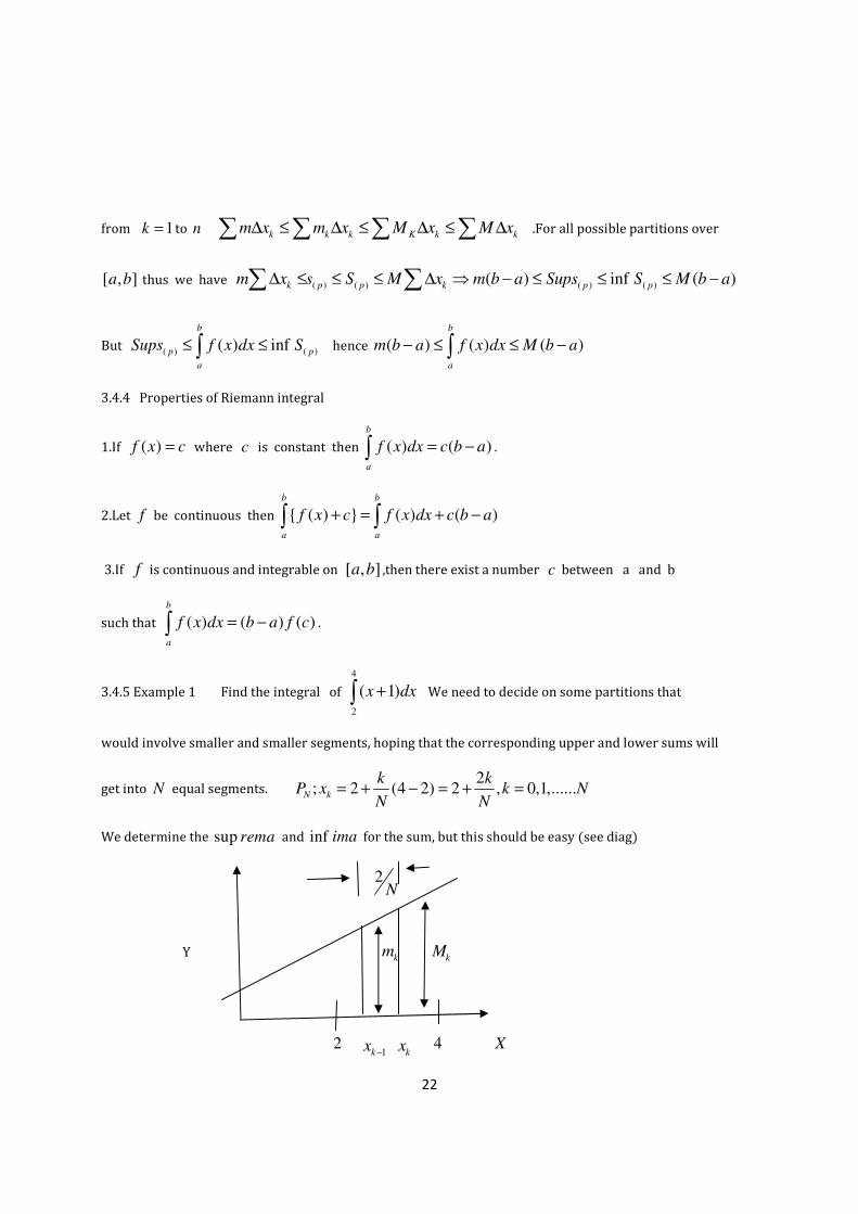
3.4.5 Example 1 Find the integral of
4
2
( 1)x dx+∫ We need to decide on some partitions that
would involve smaller and smaller segments, hoping that the corresponding upper and lower sums will
get into N equal segments. 2
; 2 (4 2) 2 , 0,1,......N k
k kP x k N
N N= + − = + =
We determine the sup rema and inf ima for the sum, but this should be easy (see diag)
2N
Y km k
M
2 1kx − k
x 4 X

23
1
1 1
2 2 2( , ) ( )( ) (( ) 1).
N N
N k k k
k k
kU f p f x x x
N n−
= =
+= − = +∑ ∑
2 2
1 1
6 4 6 4 ( 1)1 . .
2
N N
k k
N Nk N
N N N N= =
+= + = +∑ ∑
2 1
6N
N
+= +
1 1
1 1
2( 1) 2( , ) ( )( ) ((2 1).
N N
N k k k
K k
kL f p f x x x
N N− −
= =
−= − = + +∑ ∑
=2
1 1 1
6 4 41 1
N N N
K K K
KN N N= = =
− +∑ ∑ ∑
2 2
6 4 4 ( 1). . .
2
N NN N
N N N
+= − +
=4 1
6 2( )N
N N
+− +
When we send N to infinity ,the sums approximate the area as well
2 1 ( , ) lim( ( , ) lim(6 ) 8N
n n
NInf U f p U f p
N→∞ →∞
+≤ = + =
4 1
( , ) lim( ( , )) lim(6 2 ) 8Nn n
NSup U f p L f p
N N→∞ →∞
+≥ = − + =
Thus
8 ( , ) inf ( , ) 8Sup U f p U f p≤ = ≤
( , ) inf ( , ) 8Sup U f p U f p= =
Hence the function is Riemann integrable on and
4
2
( 1) 8x dx+ =∫

24
3.4.6 Example 2
Show that a constant function k is integrable and ( )
b
a
kdx k b a= −∫
For any partition p of the interval [ , ]a b ,
we have 1 2
( , ) ........n
L p f k x k x k x= ∆ + ∆ + + ∆
1 2( ........ ) ( )
nk x x x k b a= ∆ + ∆ + + ∆ = −
sup ( , ) ( )
b
a
kdx L p f k b a
−
= = −∫
inf ( , ) ( )
b
a
kdx U p f k b a
−
= = −∫
Thus ( )
b b
a a
kdx kdx k b a
−
−
= = −∫ ∫
3.4.7 Example3
Show that the function f defined by
( )f x = 0; .. .. ..
( )1; .. .. ..
when x is rationalf x
when x is irrational
=
is not integrable on any interval
Let us consider a partition p of an interval [a,b]
1 1 1 2
1
( , ) 1 1 ....... 1n
n
i
U p f M x x x x b a=
= ∆ = ∆ + ∆ + + ∆ = −∑
inf ( , )
b
a
fdx U p f b a
−
= = −∫
1 2( , ) sup0 0 ........ 0 0
nL p f x x x= ∆ + ∆ + + ∆ =
sup ( , )
b
a
fdx L p f
−
=∫
Thus b b
a a
fdx fdx
−
−
≠∫ ∫ , hence, the function f is not integrable.

25
3.5.0. Some Calculus Theorems Allied to Riemann Integral
3.5.1 Definition
Let f be differentiable and defined on ( , )a b and let f be continuous on [ , ]a b ,
If f satisfies '( ) ( ) ( , )F x f x x a b= ∀ ∈ , then F is called the anti derivative or primitive of f
3.5.2 Example
For 2( )F x x= then anti derivative of ( )f x is defined by
3
( )3
xF x c= +
3.5.3 Theorem
Let F be anti derivative for f and G be defined on [ , ]a b .Then G is a primitive for f
on [ , ]a b if and only if for some constants c , ( ) ( )G x F x c= +
Proof
( )F x c+ is a primitive of f on [ , ]a b ,suppose G is a primitive of f on [ , ]a b
then F G− is continuous and differentiable on [ , ]a b
[ ( ) ( )] '( ) '( )D F x G x F x G x⇒ − = −
'( ) '( )f x f x= −
0=
( ) ( )F x G x c⇒ − =
( ) ( )G x F x c⇒ = +

26
3.5.4 Theorem(Fundamental theorem of integral calculus)
Any function f which is continuous on [ , ]a b has a primitive on [ , ]a b .
If G is any primitive of f Then ( ) ( ) ( )
b
a
f x dx G b G a= −∫ [ ( )]b
aG t=
Proof
Let F be defined on [ , ]a b by ( ) ( )
b
a
F x f t dt= ∫ ∀ [ , ]x a b∈ ,
then ( ) ( ) ( )
b
a
f t dt F b F a= −∫
( ( ) ) ( ( ) )G b c G a c= + − +
= ( ) ( )G b G a− [ ( )]b
aG t=
3.5.5 Theorem
Let f and g be continuous on [ , ]a b and , Rλ µ ∈ ,
Then ( ( ) ( )) ( ) ( )
b b b
a a a
f x g x dx f x dx g x dxλ µ λ µ+ = +∫ ∫ ∫
Proof
Let F and G be primitive of f and g on [ , ]a b ,
then ,h F Gλ µ= + is a primitive of f gλ µ+
and ( ) ( ) [ ( ) ( )]
b
b
a
a
f t g t dt F t G tλ µ λ µ+ = +∫ by . . .F T I C
[ ( )] [ ( )]b b
a aF t G tλ µ= +
( ) ( )
b b
a a
f t dt g t dtλ µ= +∫ ∫

27
3.5.6 Theorem(Integration by parts)
Suppose f and g are continuous on [ , ]a b and have primitives F and G respectively on [ , ]a b
Then ( ) ( ) [ ( ) ( )] ( )
b b
b
a
a a
f t G t dt F t G t F t dt= −∫ ∫ where ' ( )F f x= and ' ( )G g x=
Proof
( )FG G F F G Gf Fg∆ = ∆ + ∆ = +
FG⇒ is a primitive of fG Fg+ on [ , ]a b ,by previous theorem (fundamental theorem of integral
calculus) ( ( ) ( ) ( ) ( ) [ ( ) ( )]
b
b
a
a
f t G t F t g t dt F t G t⇒ + =∫
Distributing integration signs, we have
( ) ( ) ( ) ( ) [ ( ). ( )]
b b
b
a
a a
f t G t dt F t g t dt F t G t+ =∫ ∫
( ) ( ) [ ( ) ( )] ( ) ( )
b b
b
a
a a
f t G t dt F t G t F t g t dt⇒ = −∫ ∫
, hence integration by parts.
3.5.7 Theorem (Cauchy Criterion)
Let ( )n
f be a sequence of functions defined on S R⊆
then their exist a function f ,such that nf converges uniformly on S
iff the following is satisfied,
0ε∀ > N∃ such that | ( ) ( ) |n
f x f x ε− < x s∀ ∈ and ,m n N>

28
3.5.8 Theorem (Cauchy –schwarz inequality)
Suppose f and g are continuous on [ , ]a b
then 2 2 2 ( ) ( ) ( ) . ( )
b b b
a a a
f t g t dt f t dt g t dt≤∫ ∫ ∫
Proof,
For any [ , ]x a b∈ , 2 2 2 20 ( ) ( ) ( ) 2 ( ). ( ) ( )
b b b b
a a a a
xf t g t dt x f t dt x f t g t dt g t dt≤ + = + +∫ ∫ ∫ ∫
2Ax Bx C≡ + +
i.e 2 2 0Ax Bx C+ + = , such a quadratic equation cannot have two different
Roots implies 2 4 0b ac⇒ − ≤ i. e 2 4b ac≤ Substituting ( )2 22 4B AC B AC≤ ⇒ ≤
2 2 2
( ) ( ) ( ) . ( )
b b b
a a a
f t g t dt f t dt g t dt⇒ ≤∫ ∫ ∫
3.5.9 Theorem ( . .M V T of Integral Calculus)
Let f be continuous on [ , ]a b ,then ∃ ( , )a bξ ∈ for which ( ) ( ) ( )
b
a
f x dx b a f ξ= −∫
where ( ) ( )
( )F b F a
fb a
ξ−
=−
Proof
Since f is continuous on [ , ]a b then f is Riemann integrable [ ( ) ( ) ( )]
b
a
m b a f x dx M b a− ≤ ≤ −∫
thus ∃ µ between min and max such that ( ) ( )
b
a
f t dt b aµ= −∫ , but f is continuous
and takes all the values between min and max ⇒ ∃ ( , )a bξ ∈ such that ( )f ξ µ=
i.e ( ) ( )( )
b
a
f t dt f b aξ= −∫

29
RIEMANN-STIELJES INTEGRAL
4.3.0 Review;
In Riemann integral 1 ( );
i i iM Sup f x x x x−= ≤ ≤ and 1
inf ( ); i i i
m f x x x x−= ≤ ≤ , 1i i ix x x −∆ = −
The upper and lower sums are defined by
1
( , )n
i i
i
U M x u p f=
= ∆ ≡∑ and 1
( , )n
i i
i
L m x L p f=
= ∆ ≡∑
And further ( ) inf inf ( , )
b
a
f x p fµ µ
−
= =∫ …(i) ( ) sup sup ( , )
b
a
f x dx L L p f
−
= =∫ ……(ii)
Remark. Inf and Sup taken over all possible partition P of [a, b]. If (i) and (ii) are equal
i.e ( , ) ( , )u p f L p f= then f is said to be Riemann –Integrable on [a ,b].
4.3.1 Def (R.S integrals)
Let α be a real value on which f is monotonically ( )↑ on [ , ]a b ,since ( )aα and ( )bα
are finite .It follows that α is bounded on [ , ]a b ,corresponding to each partition P of [ , ]a b
We write 1( ) ( )
i ix xα α α −∆ = − .Clearly , 0α∆ ≥ ,for any real valued function f which is
bounded on [ , ]a b , We have 1
( , , )n
i i
i
u p f Mα α=
= ∆∑ , 1
( , , )n
i i
i
L p f mα α=
= ∆∑
We define ( ) ( ) ( ) ( , , )
b b
a a
f x d x fd Inf p fα α α
− −
= =∫ ∫ and ( ) ( ) ( ) ( , , )
b b
a a
f x d x fd x SupL p fα α α
− −
= =∫ ∫
If b b
a a a
fd fd fdα α α
−
−
= =∫ ∫ ∫ ……………..(1)
Equation (1) is called the Riemann -Stieltjes integral of f with respect to α over [ , ]a b .
In this case f is said to be .R S integral and is denoted by ( )f R α∈ .

30
4.3.2 Remark
If ( )x xα = then the .R S integral reduces to Riemann integral
4.3.3 Theorem
If *P is a refinement of P ,then ( , , ) ( *, , )..( )L p f L P f iα α≤ *( , , ) ( , , )U p f U p fα α≤ …(ii)
Proof
To prove ( )i ,suppose *P contains only one point more than P and let *x be the extra point
Such that *
1i ix x x− < < where 1ix − and i
x are consecutive of P .
We put 1 1 ( ); *
iW Inf f x x x x−= < < and 2
( ); * i
W Inf f x x x x= < <
Let 1 ( );
i i iM Inf f x x x x−= < < ,then clearly 1 i
w m≥ and 2 iw m≥
And so ( *, , ) ( , , )L p f x L p f x− 1 1 2 1[ ( *) ( )] [ ( ) ( *)] [ ( ) ( )]
i i i i iw x x w x x m x xα α α α α α− −= − + − − −
1 1 2( )[ ( *) ( )] ( )[ ( ) ( *)] 0
i i i iw m x x w m x xα α α α−= − − + − − ≥
*( , , ) ( , , ) 0L p f L p fα α⇒ − ≥ ( , , ) ( *, , )L p f L p fα α⇒ ≤
4.3.4 Corollary
( ) ( ) ( ) ( )
b b
a a
f x d x f x d xα α
−
−
=∫ ∫
Proof
Let *P be the common refinement of two partition 1p and 2
p 1 2*P p p⇒ = ∪
by theorem
above *
1 2( , , ) ( , , ) ( *, , ) ( , , )L p f L p f U p f U p fα α α α≤ ≤ ≤ Hence 1 2( , , ) ( , , )L p f U p fα α≤
and if 2p is fixed and Sup taken over all possible partition 1
p
2( , , ) ( ) ( , , )
b
a
SupL p f f x dx U p fα α
−
= ≤∫

31
Thus ( ) ( )
b
a
f x d xα
−
∫ is a lower bound, taking inf imum over all possible partition 2p ,
we obtain 2( ) ( ) ( , , )
b
a
f x d x InfU p fα α≤∫
2( , , )
b b
a a
fd InfU p f fdα α α
−
−
≤ =∫ ∫ .
b b
a a
fd fdα α
−
−
⇒ ≤∫ ∫
4.3.5 Example
Let ( )x xα = and define f on [0,1] as 1; ..
( )0; ...
if rationalf x
if irrational
=
( )f b
Show that
1 1
0 0
( ) ( ) ( ) ( )f x d x f x d xα α≤∫ ∫
( )f a
mi Mi
Solutions 0 1
For every partitions of [0,1] , ( ); [0,1] 1i
M Sup f x x= ∈ = and ( ); [0,1] 0i
m Inf f x x= ∈ =
Since every sub-interval 1[ , ]
i ix x− contains both rational and irrational and this holds to
each partitions hence P∀ ( , , ) ( , ) 1u p f u p fα = = , ( , , ) ( , ) 0L p f L p fα = =
Thus 1 1
0 0
( ) ( ) ( ) ( )f x d x f x d xα α≤∫ ∫
Thus the 1
0
( ) sup ( , ) 0f x dx L p f= =∫ and 1
0
( ) ( , ) 1f x dx Inf p f= =∫ .Then we compare the two
Since 0≠1 i.e. 0<1 and then
1 1
0 0
( ) ( ) ( ) ( )f x d x f x d xα α≤∫ ∫

32
4.3.6 Theorem
( )f R α∈ on [ , ]a b if for every 0ε > ∋ partition P s. t ( , , ) ( , , )U p f L p fα α ε− < ……….*
(a criterion to show integral)
Proof
For every point P we have ( , , ) ( , , )
b b
a a
L p f fd fd U p fα α α α
−
−
≤ ≤ ≤∫ ∫
Thus 0
b b
a a
fd fdα α ε
−
−
≤ − <∫ ∫
Since ε is arbitrary chosen
b b
a a
fd fd fdα α α
−
−
= =∫ ∫ ∫ i.e f is R S− integral and ( )f R α∈
Conversely
Suppose ( )f R α∈ and let 0ε > , then there are partitions 1
p and 2
p of [ , ]a b
Such that , 2( , , )2
b
a
u p f fdε
α α− <∫ ……(i) and 1( , , )2
b
a
fd L p fε
α α− <∫ ….(ii)
Let P be common refinements of 1p and 2
p
Then 2( , , ) ( , , )
2
b
a
U p f U p f fdε
α α α≤ + ∫
Hence we have 2 1,( , , ) ( , , ) ( , )
2u p f u p f L p f
εα α α ε≤ < +
1( , , ) ( , , )u p f L p fα ε α⇒ < +
i.e. 1
( , , ) ( , , )u p f L p fα α ε− < where ( )f R α∈

33
4.3.7 Properties of R.S integration
(a)If 1( )f R α∈ , 2
( )f R α∈ on [ , ]a b then 1 2( )f f R α± ∈
by linearity . ( )c f R α∈ c R∀ ∈ .
(b)If 1 2( ) ( )
of x f x≤ then 1 2
b b
a a
f d f dα α≤∫ ∫ .
(d)If ( )f R α∈ on [ , ]a b , ( )f x M≤ , then | | [ ( ) ( )]
b
a
fd M b aα α α≤ −∫
(e)Linearity, If 1
( )f R α∈ and 2
( )f R α∈
Then 1 2 1 2( )
b b b
a a a
f fd fdα α α α+ = +∫ ∫ ∫ And ( )
b
a
f R c c fdα α∈ = ∫
Proof (e)
If 1 2f f f= + and P is any partition of [ , ]a b
We have that 1, 2( , ) ( , , ) ( , , )L p f L p f L p fα α α+ ≤ 1, 2( , , ) ( , ) ( , , ).U p f U p f U p fα α α≤ ≤ +
If 1( )f R α∈ and 2
( )f R α∈ , let 0ε > be given. There are partitions ( 1,2)jp j =
such that ( , , ) ( , , )j j j jU p f L p fα α ε− < .These inequalities persists if 1p and 2
p are
replaced by their common refinement p .Thus ( , , ) ( , , ) 2U p f L p fα α ε− < which proves
that ( )f R α∈ and for this p we have ( , , )j jU p f f dα α ε< +∫ ( 1,2)j =
1 2( , , ) 2fd U p f f d f dα α α α ε⇒ ≤ < + +∫ ∫ ∫ ,Since ε was arbitrary ,we have that
1 2fd f d f dα α α≤ +∫ ∫ ∫ …………(a) If we replace 1f and 2
f in (a)
by 1
f− and 2
f− ,the inequality is reversed and equality is proved.

34
4.4.1 Definition; Unit Step function
A function α defined on [ , ]a b is said to be a step function if ∃ a partition 0 1 , ,............,
nP x x x=
With 0 1............
na x x x b= < < < = such that α is constants on each interval.
The number ( ) ( )k kx xα α+ −− is called the jump at k
x for 1 k h< <
( )xα 3α
2α
1α
0x a=
1
x
2......x
nx b=
4.4.2 Example
0; 0( )
1; 0
xI x
x
≤=
> and in general
0;( )
1;
xI x
x
εε
ε
≤− =
> the partition provides link
between R.S integral and finite series
4.4.3 Theorem
Let α be n
f on [ , ]a b with ( ) ( )k k kx xα α α+ −= − as in above.
Let f be defined such that both f and α are not discontinued from
Right to left at each k
x then b
a
fdα∫ exists
and 1
( ) ( ) ( )
b n
k
ka
f x d x f xα=
=∑∫ .

35
4.4.4 Example (step function)
Let [ ]x be the largest integer less than or equal to x ,
referred to as greatest integer function,[x]≤x≤[x]+1 e.g. [π], [e]=2
Y
1| 2
| 3| 4
| 5|
X
Note [ ]α is continuous from the right with 1k
α = . Thus If f is continuous on [2,5] and
( ) [ ]x xα = Then 5 5
0 0
( ) ( ) ( ) [ ]f x d x f x d xα =∫ ∫ from theorem above
5
1
( ) 1 2 3 4 5 15i
f i=
= = + + + + =∑
Now suppose f was x2
2 2
5 52 2 2 2 2
10
[ ] 1 2 3 4 5i
x d iα=
= = + + + +∑∫
1 4 9 16 25 55= + + + + =
4.4.5 Example 2
5 5 5
2 2 2
0 0 0
( ( [ ]) [ ]x d x x x dx x d x+ = +∫ ∫ ∫
2 55 2
0
0
|3 i
xi
=
= +∑
125 2
1 4 9 16 25 963 3
= + + + + + =

36
4.5.0 Theorem (change of variable)
Suppose µ is a strictly increasing continuous function that maps an interval [ , ]A B onto [ , ]a b
Suppose α is monotonically increasing on [ , ]a b and ( )f R α∈ on [ , ]a b ,
Define β and g on [ , ]A B by ( ) ( ( ))y yβ α µ= ( ) ( ( ))g y f yµ= ………………..(I)
then ( )g R β∈ and
B b
A a
gd fdβ α=∫ ∫ ………….(II)
Proof
To each partition 0 1, ,.........., nP x x x= of [ , ]a b corresponds a partition 0 1 , ,........
nQ y y y= of
[ , ]A B such that ( )i i
x yϕ= and all partitions are obtained in this way .Since the values taken by f
on 1
[ , ]i i
x x− are exactly the same as those as those taken by g on 1
[ , ]i i
y y− ,we see that
( , , ) ( , , )U Q g U p fβ α= , ( , , ) ( , , )L Q g L P fβ α= …….(III).Since ( ),f R α∈
can be chosen so that both ( , , )U p f α and ( , , )L p f α are close to fdα∫ .and
( , , ) ( , , )U p f L p fα α ε− < , then ( )g R β∈ and thus B b
A a
gd fdβ α=∫ ∫ ,if ( )x xα = and
β ϕ= and if ' Rϕ ∈ on [ , ]A B then ( ) ( ( ) '( )
b B
a A
f x dx f y y dyϕ ϕ=∫ ∫
4.5.1 Example
Evaluate 2sin cosx xdx∫
solution
Let sinu x= , then cos ; cosdu
x du xdxdx
= =
Thus 2 2sin cosx xdx u dµ=∫ ∫
3
3
uc= +
3sin
3
xc= +

37
4.6.0 Integration Of Vector-Valued Functions
Let 1, 2,......... kf f f be real functions on [a, b] and 1( ,........, )
kf f f= be the corresponding
mapping of [a, b] into kR .If α increases monotonically on [a, b],to say ( )f R α∈ ,for 1,......,j k= .
in this case 1( ,........ )
b b b
k
a a a
fd f d f dα α α=∫ ∫ ∫ i. e fdα∫ is the point
in kR whose
thj co-ordinates is jf dα∫
4.6.1 Theorem
If f maps [ , ]a b into kR and ( )f R α∈ for some monotonically increasing α on [ , ]a b
Then | | ( )f R α∈ and | | | | ....( )
b b
a a
fd f d aα α≤∫ ∫
Proof
If 1..........
kf f are components of f ,then
1
2 2 21| | ( ....... )nf f f= + + ,each of 2
( )i
f R α∈
and hence does their sum. Since square root function is continuous on [0,M] for
every real M, | | ( )f R α∈ ,
To prove (a)Let 1( ,...... )
ny y y= where j jy f dα= ∫ then we have that y fdα= ∫
2 2| | j jy y y f dα⇒ = =∑ ∑ ∫ ( )j jy f= ∑∫ , by the Schwarz inequality
( ) | || ( ) |j jy f t y f t≤∑ ( )a t b≤ ≤ hence 2| | | | | | ....( )y y f d bα≤ ∫
If 0y = a is trivial, If 0y ≠ , division of (b) by | |y gives (a).

38
4.6.2 Example
If 2 2(3 6 ) 14 20A x y i yzj xz k= + − +
Evaluate .c
A dr∫ from (0,0,0) to (1,1,1) along the following paths C
where x t= , 2y t= , 3z t=
Solution
Points (0,0,0) and (1,1,1) corresponds to 0t = and 1t = respectively
dx dt= , 2dy dt= , 23dz t dt=
1
2 2. (3 6 )
t
c t o
A dr t t dt
=
=
= +∫ ∫ 2 314( )( )2t t dt− 3 2 220( )( ) 3t t t dt+
1
2 2 9
0
9 28 60t dt t dt t dt= − +∫
1
2 6 9
0
(9 28 60 )t t t dt= − +∫ 3 7 10 1
03 4 6 | 5t t t= − + =
4.6.3 Example2
Compute the length of the arc ( cos ) ( sin )t t tx e t i e t j e k= + + t−∞ < < ∞
0 0
| | | cos sin ) ( sin cos ) |
t t
t t t t tdxS dt e t e t i e t e t j e k dt
dt= = − + + +∫ ∫
1
2 2 2 2
0
[ ( 2cos sin ) (2cos sin 1) ]
t
t t te t t e t t e dt= − + + +∫
0
3 3( 1)
t
t te dt e= = −∫

39
4.7.0 Rectifiable Curves
4.7.1 Definition ;For each curve γ in kR there is associated a subset of k
R ,
i.e. the range of γ ,but different curves may have the same range.
We associate to each partition 0 1
, ,........., n
P x x x= of [ , ]a b and to each Curve γ on [ , ]a b
the number 1
1
( , ) | ( ) ( ) |n
i i
i
P x xγ γ γ −=
∧ = −∑
the thi term in this sum is the distance (in k
R )
between the points 1
( )i
xγ − and ( ).i
xγ
Hence ( , )p y∧ is the length of a polygonal path with vertices at 0 1( ), ( ),......... ( )
nx x xγ γ γ
in this order. As our partitions becomes finer and finer this polygon approaches the range of γ more
and more closely and is reasonable to define the length of γ as ( ) sup ( , )pγ γ∧ = ∧ ,
where the supre mum is taken over all partitions of [ , ]a b .
If ( )γ∧ < ∞ ,we say that γ is rectifiable.
In certain cases, ( )γ∧ is given by a Riemann integral, this can be proved for
curves γ whose derivatives 'γ is continuous.
4.7.2 Theorem
If 'γ is continuous on [ , ]a b , then γ is rectifiable and ( ) | '( ) |
b
a
t dtγ γ∧ = ∫
Proof
(i)If 1i ia x x b−≤ ≤ ≤ then
1
1 1
1| ( ) ( ) | | '( ) | | '( ) |i
i i
xx
i i
x x
x x t dt t dtγ γ γ γ− −
−− = ≤∫ ∫
Hence ( , ) | '( ) |
b
a
p t dtγ γ∧ ≤ ∫ for every partition P of [ , ]a b thus ( ) | '( ) |
b
a
t dtγ γ∧ ≤ ∫ ….(i)

40
(ii)To prove the reverse inequality let 0ε > be given, Since 'γ is uniformly continuous on [ , ]a b ,
there exist 0δ > such that | '( ) ( ) |s tγ γ ε− < if | |s t δ− < .
Let 0 1 , ,..........
nP x x x= be a partition of [ , ]a b ,with i
x δ∆ < for all i ,
If 1i ix t x− ≤ ≤ it now follows that | '( ) | | '( )
it xγ γ ε≤ +
hence
1
| '( ) | | '( ) |i
i
x
i i i
x
t dt x x xγ γ ε−
≤ ∆ + ∆∫
1
| [ '( ) '( ) '( )] |i
i
x
i i
x
t x t dt xγ γ γ ε−
= + − + ∆∫
1 1
| '( ) | | [ '( ) '( )] |i i
i i
x x
i i
x x
t dt x t dt xγ γ γ ε− −
≤ + − + ∆∫ ∫
1| ( ) ( ) | 2
i i ix x xγ γ ε−≤ − + ∆
If we add these inequalities, we obtained
| '( ) | ( , ) 2 ( )
b
a
t dt p y b aγ ε≤ ∧ + −∫
( ) 2 ( )b aγ ε≤ ∧ + − and since ε was arbitrary
Thus | '( ) | ( ).............( )
b
a
t dt iiγ γ≤ ∧∫ From (i) and (ii) we have ( ) | '( ) |
b
a
t dtγ γ∧ = ∫
4.7.3 Example 1
If ( ),x f t a t b= ≤ ≤ is a rectifiable arc, show that given an arbitrary 0δ > and 0ε > ,
there exist a subdivision 1.....
o na t t t b= < < = with polygonal approximations P such
that (i) 11,.....,
i it t n−− = (ii) | ( ) |s s p ε− < ,where s and ( )s P are the lengths
of ( )x f t= and P respectively.
Since s is the supremum of all possible ( ),s P there exists subdivisions ' ' '
1 ....o n
a t t t b= < < < =

41
with polygonal approximations 'P such that ( ')s P s ε> − .For otherwise, ( )s P s ε≤ − for all
( ),s P so that s ε− is an upper bound of the ( )s P less than the supre mum s ,not impossible.
Now the above subdivision does not satisfy (i),a finer subdivision 1....
o na t t t b= < < < =
satisfying 1( )
i it t δ−− < can be obtained by introducing additional points. But the new
polygonal arc 'P obtained this way satisfies ( ) ( ')s P s P ε≤ ≤ and therefore also | ( ) |s s P ε− <
4.7.4 Example 2
Show that a regular arc ( ),x f t= ,a t b≤ ≤ is rectifiable .
let 1....
o na t t t b= < < < = be arbitrary subdivision,
Then 1( ) | |i i
i
s P x x −= −∑ 1| ( ) ( ) |i i
i
f t f t −= −∑
1 1 2 2 1 3 1
| ( ( ) ( )) ( ( ) ( )) ( ( ) ( )) |n n n n n n
n
f t f t i f t f t j f t t k− − −= − + − + −∑
1 1 1 2 2 1 3 3 1[| ( ) ( ) | | ( ) ( ) | | ( ) ( ) |]n n n n n n
n
f t f t f t f t f t f t− − −≤ − + − + −∑
' ' ' ' ''
1 1 2 1 3 1[| ( ) | ( ) | ( ( ) | ( ) | ( ) | ( )]n n n n n n i i i
n
f t t f t t f t tθ θ θ− − −≤ − + − + −∑
where we used the mean value theorem for the ( )i
f t ,and since '( )
if t are
continuous on closed interval a t b≤ ≤ ,they are bounded on a t b≤ ≤ , say by n
M .Hence
1 2 3 1 1 2 3( ) ( ) ( ) ( )( )n n
n
s P M M M t t M M M b a−≤ + + − ≤ + + −∑
Thus the ( )s P are all bounded by 1 2 3
( )( )M M M b a+ + − and so the arc is rectifiable n
M .

42
CHAPTER FIVE
The LEBESGUE INTEGRATION
5.0 Introduction
5.1 Interval of a real line
Let I be an interval of real line and points ( , )a b , where a b< i. e I is
either of the following types ( , ),[ , ], ( , ],[ , )a b a b a b a b .Then the real number b a− is called
the length of either of these interval, we denote it by ( )Iλ , In this case I is bounded
and is of the form [ , ]a b .And the length taken as +∞.
Remark
If a b= , then the length ( ) 0Iλ = , thus the void set ∅ has a length i. e ( ) 0µ ∅ = .
5.2 .0 The Lebesgue Measure
5.2.1 Theorem
Consider R with the metric (Euclidean) then any open subsets E of the real line can be
expressed as the union of at most countable family of mutually disjoint sub-interval of R .
Proof
Let A be any subsets of the real line 'R then there is at least one open subset of R which
Contains A ( for instance R contains A ),Let this open subset be expressed as a union of
at most countable family of open sub-interval of R . Hence any subset A of R can be covered
by at most countable family of open intervals denoted by ( )S A I. e the class of all
such at most countable covers of A .
If γ is at most countable collection of open sub-interval’s of R and thus 1( )
nIγ ∞= ,
where each ( )n
I is an open interval and 1
( ), ( )n
n
I S A S Aγ∞
=
= ∀ ∈U

43
5.2.2 The Outer Lebesgue Measure
Let γ represent any at most countable collection of open sub-intervals of 'R
We put ; n
I n Nγ = ∈ ,each of nI is an open sub-Interval of 'R .such
that the non-negative extended real number *( ) ( )Iλ γ λ=∑ i. e *( )λ γ -represent’s sum
of the length’s of all sub-interval in the collection γ . Let E be any subsets of R and let γ
be any at most countable collection of open sub-interval’s that covers E which implies that
( ( ))S Eγ ∈ . The extended real number inf *( ); ( ( ))S Eλ γ γ ∈ is called the outer lebesgue
measure of E denoted by *( )m E .
Equivalently
Let ( ( ))S Eγ ∈ ,at most countable sub-interval that covers E i. e 1( )n n
Iγ ∞== , then the extended
real number *( ) ( )nIλ γ λ=∑ i. e ( )S Eγ ∈ is a set of real numbers 1 2
*( ), *( )....λ γ λ γ
Then we proceed to take the infimum, inf *( ); ( )S Eλ γ γ ∈
and *( ) inf *( ); ( )m E S Eλ γ γ= ∈ ,
Hence for each subset E of R’ there corresponds a unique non-negative extended
number *( ) 0m E ≥ and it’s infimum is such that **; ( ')T
m P R R→
extended real number is called the outer Lebesgue measure.
5.2.3 Remark ; Lebesgue measure is complete .For if EϵM and M(E)=0 and A⊆E
then AϵM and M*(A)=0
Proof ; Let M*(E)=0, and A⊆E, then by motone property M*(A) ≤M*(E)=0
*( ) 0... .. *( )o M A thus M A⇒ ≤ ≤

44
5.2.4 Theorem
Let *m denote the outer lebesgue measure on 'R
Then (i) *( ) 0m φ =
(ii) *( ) 0m E ≥ ,whenever E F∈ (non-negative)
(iii) If , ( )A B P R∈ and A B⊂ then *( ) *( )m A m B≤
monotone property of M*
Proof
(i)We choose γ φ= ⇒ ( ( ))Sγ φ∈ then *( ) 0λ γ = ( ( ))Sγ φ∀ ∈
Now *( ) inf *( ); ( ) 0m Sφ λ γ φ= =
(ii)Let 'x R∈ consider E x= then , 2 2
x xε εγ
− += covers x also
*( ) ( ) ( )2 2
n
x xI
ε ελ γ λ
+ −= = −∑ ,The measure *( ) *( )m x λ γ ε≤ =
Implying the measure of infimum is positive i.e. 0 *( *( )m x λ γ ε≤ ≤ = ,
and *( ) 0m x = if γ = ∅
(iii)Since A B⊆ , ( ) ( )S A S B⊆
Indeed if implying ( )S Bγ ∈ ,
Then *( ), ( ) *( ); ( )S A S Bλ γ γ λ γ γ∈ ⊆ ∈
and hence *( ) *( )m A m B≤

45
5.2.5 Theorem
*M is count ably sub-additive i. e if 1( )
n nE
∞−
is a sequence of subsets of 'R
then 1
*( ) *( ).........( )n
n
m m E i∞
=
≤∑U
Proof ;Suppose *( )on
m E = +∞ for some o
n N∈ ,then the right hand side of (i)
diverges, however since 1
on n
n
E E∞
=
⊆U introducing the measure 1
*( ) *( )on n
n
m E m E∞
=
≤ U
thus *( )nm E+∞ ≤ U hence(i) holds true for *( )onm E = +∞
Assume *( )nm E ≤ ∞ by definition of *m it follows that for each
0ε > ( )n S Eγ∃ ∈ such that *( ) *( ) , 1,...2
n n nm E n
ελ γ ≤ + =
Let
1
n
n
γ γ∞
=
=U then γ is atmost countable collection of open interval which covers
1
n
n
E∞
=U
1
( )n
n
S Eγ∞
=
∈ U The measure of the union
1 1
*( ) *( )n n
n n
m E λ γ∞ ∞
= =
≤U U *( )λ γ=
1
*( )n
m E∞
=U
1
*( )n
n
λ γ∞
=
≤∑1
( *( ) )2
n nn
m Eε∞
=
< +∑1
*( )n
n
m E ε∞
=
= +∑
11
*( ) *( )n n
nn
m E m E∞ ∞
==
≤∑U

46
5.2.6 Thm; If E ∉Μ then there is a subset A of E with finite positive measure (0 *( ) )m A< < ∞
Proof
Since the measure E ∉Μ by definition 'x R∃ ⊆ such that *( ) *( ) *( )cm x m x E m x E< ∩ + ∩
Suppose *( )m x E∩ = +∞ ,Since x x E⊇ ∩ by monotone property *( ) *( )m x m x E≥ ∩ = +∞
Thus *( )m x = +∞ and hence *( )m x E∩ < ∞
Next suppose *( ) 0m x E∩ = Thus *( ) *( )cm x m x E< ∩ ,
This is a contradiction since c
x x E⊇ ∩ hence *( ) *( )c
m x m x E⊇ ∩ *( ) 0m x E⇒ ∩ >
i.e 0 *( )m x E< ∩ < ∞ Putting x E A∩ = we have 0 *( )m A< < ∞ where A E⊂
5.2.7 Theorem
If ,A B∈Μ ,then so is A B∪ ,Any finite union is measurable or Μ is closed under the union operation
Proof
Let A∈Μ by definition ,it follows that any 'X R⊆ i. e *( ) *( ) *( )....( )cm x m x A m x A i= ∩ + ∩
Similarly B Y R∈Μ⇒ ∃ ⊆ such that *( ) *( ) *( )....( )cm Y m Y B m Y B ii= ∩ + ∩
In particular c
Y X A= ∩ ……. ( )iii ,using ( )iii and ( )ii we have
that *( )cm x A∩ = *( )cm x A B∩ ∩ *( ).....( )c cm x A B iv+ ∩ ∩
Substituting (iv) and (i) gives *( ) *( )m x m x A= ∩ *( )cm x A B+ ∩ ∩ + *( )c cm x A B∩ ∩
or *( ) *( ( ))m x m x A B= ∩ ∪ ( )cA B+ ∪
Hence by finite sub-additivity of m*, *( ( )m x A B∩ ∪ *( ) *( ( ))c cm x A m x A B≤ ∩ + ∩ ∩
*( ) *( ( ))m x m x A B⇒ ≥ ∩ ∪ *( ( ) )cm x A B+ ∩ ∩ x R⇒ ∃ ⊆ such that
*( ) *( ( )) *( ( ) )cm x m x A B m x A B≥ ∩ ∪ + ∩ ∪ and from definition we have A B∪ ∈ Μ

47
5.2.8 Theorem
If A and B are both L-measurable then A B∩ ∈ Μ
Proof
,A B ∈Μ from definition, ,c cA B⇒ ∈Μ ∈Μ
c c
A B⇒ ∪ ∈Μ
( )cA B⇒ ∩ ∈Μ
A B⇒ ∩ ∈ Μ
5.2.9 Definition (Ω − Algebra or Ω − Field)
Let X be a non-void set and ℱ be a class of subsets of X satisfying
the following (1) φ ∈ℱ
(2) If E ∈ℱ then c
E ∈ℱ
(3) If 1( )n nE ∞− is a sequence of members of ℱ then
1
n
n
E∞
=
∈U1
n
n
E∞
=
∈U ℱ
Then ℱ is called a Ω − algebra of subsets of X
5.2.10 Theorem (Disjoint Lemma)
Let X be a non-void set and Ω be an algebra of X
If 1( )n nE ∞
= is any sequence of sets in Ω such that
(i) n nD E⊆
(ii) m nD D∩ = ∅ whenever m n≠ where 1( )n nD ∞
= is pair wise disjoint
(iii)1 1
n n
n n
D E∞ ∞
= =
=U U ,Then x belongs to at least one of the 'n
E s

48
Proof
(i) n nD E⊆ n N∀ ∈ since n
E ∈Ω is an algebra
and 'n
D s are obtained from 'n
E s .Using operations of union of sets
on finite number of sets i. e D E= and ( 1 2..... )
nE E E∪ ∪ 1n > and clearly that n n
D E⊆
(ii) m nD D∩ = ∅ , whenever 1( )n nD ∞
= is pair wise disjoint
1D
nD 2
D
3
D 2D
From construction of 'n
D s it follows that m nD D∩ = ∅ for n m≠
(iii) 1 1
n n
n n
D E∞ ∞
= =
=U U
1E 1
D
2E 1D From construction of '
nD s it follows
2D that n mD D∩ = ∅ for n m≠ thus n n
D E⊆
1 1
n n
n n
D E∞ ∞
= =
⇒ ⊆U U ,the reverse inequality is clear from (i) and 1 1
n n
n n
D E∞ ∞
= =
=U U
Since ,
1
n
n
X E∞
=
∈U then x belongs to at least one of the 'n
E s

49
5.3.0 The Lebesgue Integral For Non-negative Simple Functions
5.3.1 Definition , Indicator or Characteristic Functions
Let ( , )FΩ be a measurable space for a set A ⊆ Ω define
0,1A
X → by 0;
( )1;A
x Ax
x Aχ
∈=
∉ this function is called the characteristic
or the indicator function of a set. If Af I= where i. e ;
A eI RΩ →
and 1;
( )0;
A
x AI x
x A
∈=
∉ and
( ) 1. ( ) 0. ( )c
A x d A Aχ µ µ µ= +∫
5.3.2 Defination ; Simple Functions
Suppose the range of S consists of the distinct numbers 1 2, .........
na a a
define simple non-negative function ;e
S RΩ → by 1
( ) ( )i
n
i A
i
S x a xχ=
=∑ where 0,i i
a A F≥ ∀ ∈
and 1
i
i
A∞
=
∈ΩU , with 0i j
A A =I i j≠ .
5.3.3 Example
Consider ([0,1], , )µΜ ,define 1; .. .. ..
( )0; .. .. ..
if x is rationalf x
if x is irrational
=
.
This is a simple function with 1[0,1]A Q= ∩ and 2 1 [0,1]c cA A Q= = ∩
Note that f ∈Μ and [0,1]
1. ( [0,1])fd Qµ µ= ∩∫ 0. ( [0,1]) 0cQµ+ ∩ =
since rational s are countable then ( [0,1]) 0Qµ ∩ =

50
5.4.0 Lebesgue Integration
5.4.1 Lebesgue Integral Of Non-negative Simple Functions
Integration is defined on a measure X in which F is the ringΩ − of measurable sets and µ
is the measure on it. Suppose
1
( ) ( )i
n
i A
i
S x a xχ=
=∑ where iA F∀ ∈
,1
i
i
A∞
=
= ΩU and
0i
a R≥ ∈ is measurable and if S is measurable space ( , , )F µΩ and non-negative,
we define
1
( ) ( )n
i i
i
S x d a A Sdµ µ µ=
= =∑∫ ∫ or ( )E
E
Sd SupI sµ =∫ ………………(a)
The left side of (a) is the lebesgue integral of S ,with respect to µ over the set E
5.4.2 Properties Of The Integral
1. The integral is a non-negative extended real number 0 Sdµ≤ ≤ +∞∫
2. If 1 2 0, ,s s s L+∈ and
eRα ∈ such that 0α ≥ , the
(a) 0s Lα +∈ and ( )s d sdα µ α µ=∫ ∫
(b) 1 2 0s s L
++ ∈ then 1 2 1 2( )s s d s d s dµ µ µ+ = +∫ ∫ ∫
(c)If 1 2
s s≤ then 1 2s d s dµ µ≤∫ ∫
(d)If , 1n
s n ≥ is an increasing sequence functions in 0L+ such that lim ( ) ( )n
nS x s x
→∞=
x R∀ ∈ then ( ) ( ) lim ( ) ( )nn
s x d x s x d xµ µ→∞
=∫ ∫

51
5.5.0 The Integral Of a Non-Negative Measurable Functions
5.5.1 Definition
Let ( , )FΩ be a measurable space ,the non-negative functions ;e
f RΩ → is said to be
F − measurable, If ∃ an increasing sequence ; 1n
S n ≥ such that lim ( ) ( )nn
S x f x→∞
=
x∀ ∈Ω , we shall denote the class of all non-negative measurable function by L+ .
5.5.2 Theorem
(a)Suppose f is measurable and nonnegative on X .For A∈ Μ , define
( )A
A fdφ µ= ∫ , then φ is count ably additive on Μ
(b)The same conclusion holds if ( )f L µ∈ on X
Proof
To show 1
( ) ( )n
n
A Aφ φ∞
=
=∑ , In general case, we have ,for every measurable simple
functions S such that 0 s f≤ ≤ ,1 1
( )
n
n
n nA A
sd sd Aµ µ φ∞ ∞
= =
= ≤∑ ∑∫ ∫ 1
( ) ( )n
n
A Aφ φ∞
=
∴ ≤∑
Now if ( )n
Aφ = +∞ for some n, is trivial ,since ( ) ( )n
A Aφ φ≥
suppose ( )n
Aφ < ∞ for every n ,such that 1 2 1 2( ) ( ) ( )A A A Aφ φ φ∪ ≠≥ +
it now follows that for every n 1( ...... ) ( ) ...... ( )
n nA A A Aφ φ φ∪ ∪ ≥ + + since
1......
nA A A⊃ ∪ ∪
1
( ) ( )n
n
A Aφ φ∞
=
⇒ ≥∑
5.5.3 Definition ;For a function f L+∈ , we define the integral of f with respect t o µ
by ( ) ( ) lim ( )nn
f x d x S x d xµ µ→∞
=∫ ∫

52
5.5.4 Properties Of the Integrals
Let 1 2 3, ,f f f then the following holds
1. 0fdµ ≥∫ and for 1 2f f≥ 1 2f d f dµ µ⇒ ≥∫ ∫
2.For , 0α β ≥ , we have 1 2f f Lα α ++ ∈
and 1 2 1 2( )f f d f d f dα β µ α µ β µ+ = +∫ ∫ ∫ 1 2f d f dα µ β µ= +∫ ∫
3.For every E F∈ , we have E f Lχ +∈ and if υ ( )E = E fdχ µ∫ is a measure on F
And ( ) 0Eυ = iff ( ) 0Eµ = , the integral E
E
fd fdχ µ µ=∫ ∫ .
5.6.0 Monotone Convergence Theorem( . .M C T theorem)
Let ( , , )X µℵ be a measure space , ( )n
f be a sequence on *( , )M X ℵ s. t 1n nf f +≤ n N∀ ∈
and n
f f→ point wise on X , then 1( )n nf dµ ∞=∫ converges to fdµ∫ in
eR i. e
lim (lim )n nn n
f d f d fdµ µ µ→∞ →∞
= =∫ ∫ ∫
Proof
*(n
f m x∈ ,) n R∀ ∈ and nf f→ point wise on X *( , )f m X χ⇒ ∈
since 1n n
f f f+≤ ≤ by monotone properties of S , we have that 1 ...( )n nf d f d fd iµ µ µ+≤ ≤∫ ∫ ∫
Thus the sequence 1( )n nf dµ ∞=∫ is increasing in *
eR and hence

53
Conversely, If ; ( )n n
A x X x f xαφ= ∈ ≤ it can be shown that n
A ∈ℵ n N∀ ∈
Moreover (i) 1n nA A +⊆ (ii)
1
n
n
A X∞
=
=U
Since integral is a count ably additive set function ( ) ( )n
x f xαφ ≤ on n
x A∈ ,
by monotone property of ∫ on m*(x,ℵ ) , nd f dαφ µ µ≤∫ ∫
i.e
n
n n
A x
d f d f d fdα φ µ µ µ µ≤ ≤ ≤∫ ∫ ∫ ∫ …………(ii)
the two inequalities proof the theorem.
Remark; If we define ;λ ℵ eR→ by ( )
E
E dλ φ µ= ∫ E∀ ∈ ℵ
The ( )Eλ is a measure and therefore λ is continuous from below.
Proof
0
1i
n
i A
i
L aφ φ χ+
=
∈ ⇒ =∑ , 1
n
i
i
A=
= ΩU
1
I
n
E i A E
i
E F aφχ χ χ=
∈ ⇒ =∑ =1
i
n
i A E
i
a χ ∩=∑
where ( ) EE dλ φχ µ= ∫1
( )n
i i
i
a A Eµ=
= ∩∑ is it a measure or not
(i)1
( ) ( )n
i
i
a Aλ φ µ=
= ∩∅∑1
( ) 0n
i
i
a µ=
= ∅ =∑
(ii)Since 0i
a ≥ and ( ) 0i
A Eµ ∩ ≥ 1
( ) 0n
i i
i
a A Eµ=
⇒ ∩ ≥∑

54
(iii) λ is countable additive ,for let 1
;j j
j
E E E F∞
=
= ∈U for each j
then to show that 1
( ) ( )j
j
E Eλ λ∞
=
=∑
1
( ) ( )n
i i j
i
E a A Eλ µ=
= ∩∑1 1
( )n
n i j
j j
a A Eµ∞
= =
= ∩∑ U
1 1
( ( ))n
i i j
i j
a A Eµ∞
= =
= ∩∑ U1 1
( )n
i i j
i j
a A Eµ∞
= =
= ∩∑ ∑
1
( )i i j
j
a A Eµ∞
=
= ∩∑∑1
( )j
j
Eλ∞
=
=∑
( )Eλ∴ is a measure.
5.6.1 Some Applications Of M.C.T.
Theorem; Let ( , , )X µℵ be a measure space and *( , )m X ℵ and C non-negative
real ,then (i) cfd c fdµ µ=∫ ∫ (ii) ( )f g d fd gdµ µ µ+ = +∫ ∫ ∫
Proof
Let ( )n
φ , ( )n
ψ be increasing ( )↑ sequence of simple ( ) *( , )n
f s M X∈ ℵ such
that ( ) ( )n increasesφ ↑ to f and ( ) ( )n increases toψ ↑ g .
ncφ⇒ is increasing sequence by M.C.T , lim (lim )n n n n
n nd d fdφ φ µ
→∞ →∞= =∫ ∫ ∫
lim nn
c dn cfdφ µ→∞
=∫ ∫ ………….* But nc d c fdφ µ µ=∫ ∫
lim limn nn n
c d c dφ µ φ µ→∞ →∞
∴ =∫ ∫ lim ......**nn
c d c fdφ µ µ→∞
= =∫ ∫
Thus from * and ** we have cfd c fdµ µ=∫ ∫ .
55
(ii) by M.C.T lim (lim )n nn n
d d gdψ µ ψ µ µ→∞ →∞
= =∫ ∫ ∫
Now ( )n n
φ ψ+ increases ( )↑ to f g+ by M.C.T
lim ( ) ( ) .....*n nn
d f g dφ ψ µ µ→∞
+ = +∫ ∫
Since nφ and n
ψ are simple ' *( , )n
f s M X∈ ℵ
( )n n n nd d dφ ψ µ φ µ ψ µ+ = +∫ ∫ ∫
Thus lim ( ) ......**n nn
d fd gdφ ψ µ µ µ→∞
+ = +∫ ∫ ∫
From * and ** we have ( )f g d fd gdµ µ µ+ = +∫ ∫ ∫
5.6.2 Example
Let ( , ( ), )R B R µ be a measurable space , where µ is the lebesgue measure on ( )B R
Let (0, )n nf χ= n N∀ ∈ ,where
nf is monotonic increasing to
[0, ]f χ +∞∈
and nf and f are ( )B R measurable functions
[0, ] [0, ]n nf d d n nµ χ µ µ= = =∫ ∫
and [0, ] ([0, ])nfd dµ χ µ µ= = +∞ = ∞∫ ∫
Now fdµ = +∫ limn
n→∞
∞ = = +∞ and ∴ M.C.T applies.

56
5.7.0 Fatou’s Lemma
Let ( ,X ℵ , )µ be a measure space ,
and ( )n
f be a sequence of elements of *(M x ,ℵ ),
Then (lim ) limn nn n
f d f dµ µ→∞ →∞
≤∫ ∫
Proof
For each n N∈ ,let 1inf , ,........
n n nf f f += ,
clearly *(nf M x∈ ,ℵ ) n N∀ ∈ and ( ) limn nn
f f→∞
↑=
Hence by M.C.T lim (lim )n nn n
f d f dµ µ→∞ →∞
=∫ ∫
i.e (lim ) lim ........*n nn n
f d f dµ µ→∞ →∞
=∫ ∫
now m nf f≤ m n∀ ≤
By monotone property n mf d f dµ µ≤∫ ∫
Taking the limits
lim lim .........**m nm n
f d f dµ µ→∞ →∞
≤∫ ∫
from * and **, we have (lim ) limn nn n
f d fµ→∞ →∞
≤∫ ∫

57
5.7.1 Theorem
Let ( ,X ℵ , )µ be a measure space and *
, (f g M x∈ , )µ and f g≤
Let E and F ∈ ℵ such that E F⊆ then(i) fd gdµ µ≤∫ ∫ and (ii) E F
fd fdµ µ≤∫ ∫
Proof
(i)If *( ,M xφ ∈ ℵ ) is simple and fφ ≤ then gφ ≤ ,further if ( )fΩ is a set of all simple
functions ,such that fφ ≤ then ( )gφ ∈Ω ( simple functions s. t gφ ≤ ) i. e ( ) ( )f gΩ ∈Ω
and hence ( ) ( )f g
Sup d Sup dφ µ φ µΩ Ω
≤∫ ∫ i. e fd gdµ µ≤∫ ∫
(ii)Consider *; ( , )E FfX fX M x∈ ℵ ) Since E F⊆ , E FfX fX⇒ ≤
By part (i) and monotony E FfX d fX dµ µ≤∫ ∫ andE F
fd fdµ µ≤∫ ∫
5.7.2 Example
Consider ([0,1], , )F µ ,and take 1 2
[ , ]n
n n
g nχ=
Note that 0n
g → in [0,1], now 1 2[ , ]
.n
n n
g dn n dnχ=∫ ∫ =1 2 1
([ , ]) . 1n nn n n
µ = =
lim lim1 1nn n
g dµ→∞ →∞
⇒ = =∫ Such that 0 lim n nn
gdn g d→∞
= ≠∫ ∫ ,M.C.T. does not apply
Now 0n
g → on [0,1], i.e (liminf ) 0 0nn
g d dµ µ→∞
= =∫ ∫
And liminf liminf 1 1nn n
g dµ→∞ →∞
= =∫ ∴ (liminf ) 0 liminfn nn n
g g dµ→∞ →∞
= ≤∫ ∫ ,
fatou’s lemma apply

58
5.8.0 Lebesgue Dominated Convergence Theorem(L.D.C.T)
Suppose 1( )
nf
∞ is a sequence of measurable functions which converges . ,a eµ to a function f .
Let g be an integrable functions such that | |n
f g≤ Then f is integrable and lim nn
f d fdµ µ→∞
=∫ ∫ ,
the function g is called a dominating function for the sequence 1( ) .nf∞
Proof.
Since 0n
f g+ ≥ , fatou’s lemma shows that ( ) liminf ( )nn
E
f g d f g dµ µ→∞
+ ≤ +∫ ∫ e
liminf ...( )nn
E
fd f d iµ µ→∞
≤∫ ∫ Since 0n
g f− ≥ similarly
( ) liminf ( )nn
E
g f d g f dµ µ→∞
− ≤ −∫ ∫
liminf[ ]nn
E E
fd f dµ µ→∞
− ≤ −∫ ∫
which is the same as lim nn
E E
fd Sup f dµ µ→∞
≥∫ ∫ …(ii) From (i) and (ii) we have lim nn
E E
f d fdµ µ→∞
=∫ ∫
5.8.1 Example . Let 1
[0, ]n
n
f nχ= for 1, 2,3,n = ,….,This functions 1; (0; )
( )0;
n
n xnf x
otherwises
∈=
,
hence ( )n
f x cannot be dominated by a single integrable functions .Further at any point in (0,1]
the sequence contains only finite number of non-zero terms and indefinite number of zeros and at
any point outside (0,1], each term of the sequence is zero Hence lim ( ) 0nn
f x→∞
= for all x n∈ ,
Thus we have Further
1
1(0, )
0
1 1((0, ] . 1
n
n
nR
f xdx n dx n dx nm nn n
χ= = = = =∫ ∫ ∫
,Thus ( ) 1n
R
f x dx =∫ for all .Hence lim 1 0 lim ( )n nn n
R R
f dx f x dx→∞ →∞
= ≠ =∫ ∫ .

59
5.8.2 Example2
Show that 1
0
lim ( ) 0nn
f x→∞
=∫ ,where 2 21
n
nxf
n x=
+
Sol
Let 2 21
2
n xnx
+= so that
2 2
1
1
nx
n x n<
+
Let 1
( )2
g x = . since a constant is integrable, ( )g x is integrable
Hence 2 2
( ) ( )1
n
nxf x g x
n x= <
+ , ( )
nf x is dominated by an integrable function ( )g x
Further 2 2
lim ( ) lim 01
nn n
nxf x
n x→∞ →∞= =
+ , So that fn(x)→0 as n→∞
Hence by lebesgue’s dominated convergence theorem
1 1
2 2
0 0
lim 0 01n
nxdx dx
n x→∞= =
+∫ ∫
5.8.3 Properties Of Lebesgue Integral For Bounded Measurable Functions
(a)If f is measurable and bounded on E , and ( )Eµ < ∞ , then ( )f µ∈l on E
(b)If ( )a f x b≤ ≤ for x E∈ , and ( )Eµ < +∞ , then ( ) ( )E
a E fd b Eµ µ µ≤ ≤∫ .
(c )If f and ( )g µ∈l on E and if ( ) ( )f x g x≤ for x E∈ then E E
fd gdµ µ≤∫ ∫
(d)If ( )f µ∈l on E , then ( )cf µ∈l on E , and E E
cfd c fdµ µ=∫ ∫
(e)If ( )f µ∈l on E and A E⊂ then ( )f µ∈l on A .

60
CHAPTER SIX
COMPARISON OF RIEMANN INTEGRAL AND LIBESGUE INTEGRAL THEORIES
6.1.0 Theorem(Equivalence of Riemann and Lebesgue)
(a) If f R∈ on [a, b], the f L∈ on [a, b] and
b b
a a
fdx R f dx=∫ ∫ .
(b) Suppose f is bounded on [ , ]a b ,the f R∈ on [ , ]a b if and only if f
is continuous almost everywhere on [ , ].a b
Proof ;(a)Suppose f is bounded , then there is a sequence kp of partitions of [ , ]a b such that
1 kp + such that the distance between the adjacent points of
kP is less than 1
kand such that
lim ( , ) ,kn
L p f R fdx→∞
−
= ∫ lim ( , )kn
U p f R fdx
−
→∞= ∫ , all the integrals are taken over [ , ]a b .
If 1 , ,...... k o np x x x= with ox a= and nx b= define ,Putting ( )k iU a M= and ( )k iL a m= for
1i ix x x− < < ,1 i n≤ ≤ and hence ( , ) ,k kL p f L dx= ∫ ( , )k k kU p f U dx= ∫ so that
1 2 2 1( ) ( ) ........ ( )...... ( ) ( )L x L x f x U x U x≤ ≤ ≤ for all [ , ],x a b∈ since 1kp + refines kp .Thus there exist
( ) lim ( )kk
L x L x→∞
=,
lim ( )k kn
U U x→∞
= and we observe that L and U are bounded and measurable
functions on [ , ]a b that ( ) ( ) ( )L x f x U x≤ ≤ where ( )a x b≤ ≤ ,and that ,Ldx R fdx−
=∫ ∫
Udx R fdx
−
=∫ ∫ , by the monotone convergence theorem, where the only assumption is that f is a
bounded real function on [ , ]a b .We note that f R∈ , if and only if its upper and lower
Riemann integrals are equal. hence if and only if Ldx Udx=∫ ∫ , since L U≤ , Ldx Udx=∫ ∫
happens if and only if ( ) ( )L x U x= for all [ , ],x a b∈
in this case ( ) ( ) ( ) ( ) ( ) ( )L x f x U x L x f x U x≤ ≤ ⇒ = =
almost everywhere on [ , ]a b , so that f is measurable, thus
b b
a a
fdx R fdx=∫ ∫

61
(b)Furthermore ,if x belongs to number kp ,it is quite easy to see that ( ) ( )U x L x= if and only
if f is continuous at x .Since the union of sets kP is countable, it’s measure is 0,and we
conclude that f is continuous almost everywhere on [ , ]a b if and only if ( ) ( )L x U x= almost
everywhere, Hence
b b
a a
fdx R fdx=∫ ∫ if and only if f R∈ .This completes the proof.
6.1.1 Example ; Evaluate
5
0
0;0 1
( ) 1; 1 2 3 4
2; 2 3 4 5
x
f x dx x x
x x
≤ ≤
= ≤ ≤ ∪ ≤ ≤ ≤ ≤ ∪ ≤ ≤
∫ by using the Riemann
and Libesgue definitions of integrals.
(I)Using Riemann definition of the integrals(where the subdivisions is taken of the segments [ , ]a b )
by the subdivisions points 0 1 2, , ,........ nx x x x on X − axis.
Y
0
1
2
3
4
5
X
the upper and lower Riemann sums tends to common value
0(1 0) 1(2 1) 2(3 2) 1(4 3) 2(5 4) 6− + − + − + − + − = thus ( ) 6
b
a
R f x dx =∫
(II)Evaluating the lebesgue integral where the sub-divisions is that of the interval [0,2 ], 0δ δ+ ≥
we get ,0[1 0] 1[(2 1) (4 3)] 2[(3 2) (5 4)] 6− + − + − + − + − = thus
5
0
( ) 6L f x dx =∫

62
6.1.2 Example 2
Let f be defined on [ , ]a b as follows 0; .. ..
( )1; .. .. ..
if x rationalf x
if x is irrational
=
, prove that f is
lebesgue integrable but not Riemann integrable.
Solution
Consider a partition 1 , ........ oP a x x x b= = < < < = of [ , ]a b .Then 1iM = in
1[ , ]i ix x−
and 0im = in 1[ , ]ix x− ,Hence 1( )p i iS x x b a−= − = −∑ and
10( ) 0p i is x x −= − =∑
so that R ( ) ( )
b
a
R f x dx b a
−
= −∫ and ( ) 0
b
a
R f x dx−
=∫ .This shows that f is not Riemann
integrable. We prove that f is lebesgue integrable.
Let Q be the set of all rationales’ in [ , ]a b ,then CQ is the set of irrationals in [ , ]a b ,where
[ , ]a b Q CQ= ∪ and Q CQ∩ = ∅ .Since Q is countable set it has a measure and hence
it is measurable in [ , ]a b and since the complement of a set is measurable, CQ is measurable.
By definitions f is the characteristic functions of CQ ,Since CQ is measurable,
f is measurable function. As f is bounded, it is integrable.
The lebesgue integral of f is
b
a Q CQ Q CQ
fdx fdx fdx fdx∪
= = +∫ ∫ ∫ ∫
as 0. ( ) 1 ( ) ( )Q CQ m Q m CQ m CQ∩ = + = .Next we find the measure CQ
If 1E and
2E are disjoint measurable sets then 1 2 1 2 1 2( ) ( ) ( ) ( )m E m E m E E m E E+ = ∪ + ∩
where 1E Q= and 2 ,E CQ= taking ( ) ( ) ([ , ]) ( )m Q m CQ m a b m+ = + ∅ , since ( ) 0m ∅ = we have
( ) ( ),m CQ b a= − thus ( )
b
a
fdx b a= −∫ .Hence f is lebesgue integrable but not Riemann Integrable.
63
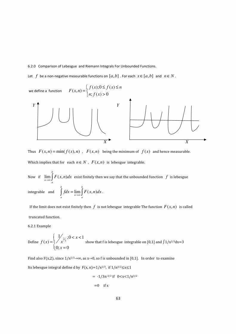
6.2.0 Comparison of Lebesgue and Riemann Integrals For Unbounded Functions.
Let f be a non-negative measurable functions on [ , ]a b . For each [ , ]x a b∈ and n N∈ .
we define a function ( );0 ( )
( , ); ( ) 0
f x f x nF x n
n f x
≤ ≤=
>
Y Y
X X
Thus ( , ) min( ( ), )F x n f x n= , ( , )F x n being the minimum of ( )f x and hence measurable.
Which implies that for each n N∈ , ( , )F x n is lebesgue integrable.
Now if lim ( , )
b
na
F x n dx→∞ ∫ exist finitely then we say that the unbounded function f is lebesgue
integrable and lim ( , )
b b
na a
fdx F x n dx→∞
=∫ ∫ .
If the limit does not exist finitely then f is not lebesgue integrable The function ( , )F x n is called
truncated function.
6.2.1 Example
Define 2
3
1 ;0 1( )
0; 0
xxf x
x
< <= =
show that f is lebesgue integrable on [0,1] and ∫1/x2/3dx=3
Find also F(x,2), since 1/x2/3→∞, as x→0, so f is unbounded in [0,1]. In order to examine
Its lebesgue integral define d by F(x, n)=1/x2/3, if 1/n3/2≤x≤1
= -1/3n-3/2 if 0<x<1/n3/2
=0 if x

64
For n=2
2 33 2
32
32
1 1, 12
1 1( ,2) , ,03
0, , 0
if xx
F x n if xn
if x
−
≤ ≤
= − < < =
Now
32
32
1(
1 1
10 0
( , ) ( , ) ( , )n
n
F x n dx F x n dx F x n dx= +∫ ∫ ∫
12
1
13
22
3103
2
1 1
3
n
n
n dx dxx
−= − +∫ ∫
13
32
1 13(1 ( )
n n= + −
23 , n
n= − ∀
Thus by the definition of lebesgue integral of unbounded functions ,we have
2
( ) lim ( , ) lim(3 ) 3n n
f x dx F x n dxn→∞ →∞
= = − =∫ ∫
6.2.2 REMARK
The Riemann integral of f on unbounded set A can exist even though the Riemann integral of | |f does
not exist on A . For example,
0
sin sinlim
b
na
x xR dx R dx
x x
∞
→∞=∫ ∫ exists as an improper Riemann integral
wheres the integral
0
sin| |
xdx
x
∞
∫ does not exist. On the contrary the lebesgue integral of
0
sin xL dx
x
∞
∫ does
not exist because
0
sin| |
xdx
x
∞
∫ does not exist ,It shows that there exists improper Riemann integrals
which are not integrable in lebesgue sense. This Indicates that nothing can be said about the equality of
the two integrals when A is unbounded, Riemann integrals may exists when the lebesgue integral does not
exists. Moreover if | |f is Riemann integrable on A , then f is both Riemann and Lebesgue integrable
on A and the two integrals are equal.

65
6.3.0 (III)Libesgue and Riemann Integrals and The Connection Between Integration And Different ion.
6.3.1 Definition, Let an interval of ( , )R a b be divided into N equal parts each of length b a
xN
−∆ =
Y
a i x+ ∆
a 2a x+ ∆ ix ( 1)b a i x= + + ∆
X
Let [ , ( 1) ]x a i x a i x∈ + ∆ + + ∆ then 0
1
lim ( )N
ix
i
f x x∆ →
=
∆∑ as N →∞ is called the de^inite
integral of f(x) in the interval ( , )a b and is denoted by ( )
b
a
f x dx∫ .
6.3.2 Theorem(fundamental theorem of differential calculus)
Let ( )f x have anti derivatives ( )F x in the interval [ , ]a b Then ( ) ( ) ( )F b F a f x dx− = ∫ .
proof, Let ( )F x be the anti derivatives of ( )f x the from mean value theorem
1 0 0( ) ( ) '( )F x F x F c x− = ∆
2 1 1( ) ( ) '( )F x F x F c x− = ∆
1
1
( ) ( ) '( )
( ) ( ) '( )
n n n
n n i
F x F x F c x
F x F x F c x
+
+
− = ∆
− = ∆ which implies ( ) ( ) ( )
b
a
F b F a F x dx− = ∫ .
6.3.3 Connection ;This familiar connection between integration and differentiation is carried over into
lebesgue theory. For if f ∈l on [ , ]a b and ( ) ( )F x f t dt= ∫ (a<x<b), then '( ) ( )F x f x= almost
everywhere on [a,b].Conversely, If F is differentiable at every point on [ , ]a b almost everywhere not
good enough And if ' [ , ]F L a b∈ then ( ) ( ) '( )
b
a
F b F a F t− = ∫ ( )a x b≤ ≤

66
6.3.4 Theorem
Let f be continuous function on [a, b], Then (i) f is integrable on [a b]
(ii)If F(x)= ( )
x
a
f t dt∫ ,where ,a x b< < then ( )F x is differentiable and '( ) ( )F x f x= .
Proof
(i)Since f is continuous on [a,b],it is measurable on [a,b]
As a continuous functions is bounded on, let | |f M≤ ,taking g M= in the property, thus
f is integrable on [a,b].
(ii)Let [ , ]A a x= , [ , ]B x x h= + so that [ , ]A B a x h∪ = +
Now we have ,
x x h
A B a x
fdx fdx fdx
+
∪
= +∫ ∫ ∫ using notation ( ),F x we have
( ) ( ) ,
x h
x
F x h F x fdx
+
+ = + ∫ which gives ( ) ( ) ( ),....( )
x h
x
F x h F x f t i
+
+ − = ∫
Since f is continuous function and the measure is the lebesgue measure,
we obtained earlier that ( , ) ( ) ( , )
x h
x
m x x h f t dt x x h M
+
+ ≤ ≤ +∫ where ( )L f t M≤ ≤
and [ , ]t x x h∈ + , For L and M are bounds of continuous function f on [a,b].
Hence there is a point ε in[ , ]x x h+ such that ( ) ....(2)
x h
x
f t dt hf ε+
=∫ where xε θ= + .
using (1) and (2) we have that ( ) ( ) ( ),F x h F x hf ε+ − = since 0h ≠ dividing by
h and taking the limits as 0,h → we have ( ) ( )
lim ( )h
F x h F xf x
h→∞
+ −=
which proves that '( ) ( )F x f x=
In term of recovery of derivative functions the two integral are are effective.

67
6.4.0 (IV) Functions Of Class 2
L
As an application of the lebesgue theory, perseval theorem and Bessels theorem already proved for
Riemann integrable functions are extended to lebesgue functions.
Definitions
A trigonometric polynomials is a finite sum of the form
( )f x a= ( ) ( cos sin )N
o n n
N
f x a a nx b nx−
= + +∑ ( )x real−
Where 1.......... , ............o N N
a a b b are complete numbers, the sum can also
be written in the form ( )N
inx
n
N
f x c e−
=∑ ( )x real−
6.4.1 Definitions
We say a sequence of complex functions n
φ is an orthonormal set of functions on a measurable
Space x if n m
x
dφ φ µ∫ = 0;( )
1;( )
n m
n m
≠
= ,in particular ,we must have
2 ( )n
φ µ= l , If 2( )f µ∈ l
and If n n
x
c f dφ µ= ∫ (n=1,2,3,…………..),we write f ~ 1
n n
n
c φ∞
=∑ .
The definitions of trigonometric Fourier series in 2L (or even to L ) on ( , )π π−
6.4.2 Theorem(Bessel Inequality)
If n
φ is an ortho normal on [ , ]a b and if ( )f x ~1
( )n n
n
c xφ∞
=∑
Then 2 2
1
| | | ( ) |
b
n
n a
c f x dx∞
=
≤∑ ∫ ,in particular lim 0n
nc
→∞= ,
The bessel inequality hold for any 2 ( )f µ∈ l .

68
6.4.3 Parseval’s Theorem(Riemann version).
Suppose f and g are Riemann integrable functions with period 2π , and ( )f x ~inx
nc e∞
−∞∑ ,
,
( )g x ~ inx
neγ
∞
−∞∑ , Then 21
lim | ( ) ( ; ) | 02
Nn
f x S f x dx
π
ππ→∞−
− =∫
_ _1
( ) ( )2
n nf x g x dx c
π
π
γπ
∞
−∞−
=∑∫
2 21| ( ) | | |
2n
f x dx c
π
ππ
∞
−∞−
=∑∫
Proof
Using the notation 1
22
1|| || | ( ) |
2h h x dx
π
ππ −
= ∫ let 0ε > be given. Since f R∈ and ( ) ( )f fπ π= − ,
by construction we obtain a continuous 2π − periodic function h with || ||f h ε− < and we find a
trigonometric polynomials P such that | ( ) ( ) |h x p x ε− < for all x .
Hence || ||h p ε− < .If P has degree No. Thus 2|| ( ) || || ||N
h S h h p ε− ≤ − < , for all 0N N≥ .
by bessel’s inequality w ith h f− in place of f , 2 2 2|| ( ) ( ) || || ( ) || || ||
N N NS h S f S h f h f ε− = − ≤ − <
Now applying triangle inequality shows that 2|| ( ) || 3
Nf S f ε− <
0N N≥
Thus 21lim | ( ) ( ; ) | 0
2N
nf x S f x dx
π
ππ→∞−
− =∫
Next _ _ _1 1
( ) ( )2 2
N Ninx
N n n n
N N
S f gdx c e g x dx c
π π
π π
γπ π− −− −
= =∑ ∑∫ ∫
And the Schwarz inequality shows that
|1_ _
2 2| ( ) | | ( ) || | | | | | N N Nf g S f g f S f g f S g− ≤ − ≤ −∫ ∫ ∫ ∫ ∫ ,
which tends to zero as N→∞ ,if g f=

69
6.4.4 Parseval Theorem For 2
( )f µ∈l lebesgue version
Suppose ( )f x ~inx
nc e
∞
−∞∑ …..(a) ,where 2
f ∈ l on [ , ]π π−
Let n
S be the partial sum of (a), Then lim || || 0n
nf S
→∞− =
And 2 21| | | |
2n
c f dx
π
ππ
∞
−∞ −
=∑ ∫
Proof
Let 0ε > be given ,since 1
2 2|| || ( )
b
a
f g f g dx ε− = − <∫ , there is a continuous function g
such that || ||2
f gε
− < .Moreover, we can arrange it so that ( ) ( )g gπ π= − ,then g
can be extended to a Periodic continuous function by Perseval Riemann version(earlier),
there is a trigonometric polynomial T ,of degree N ,say, such that || ||2
g Tε
− < .
Hence by Bessels inequality (extended to 2l ), n N≥ implies || || || ||
nS f T f ε− ≤ − <
thus lim || || 0n
nf S
→∞− = and hence
2 21| | | |
2nc f dx
π
∞∞
−∞ −∞
=∑ ∫ , as proved in perseval Riemann version.
6.4.5 Corollary
If 2f ∈ l on [ , ]π π− and if ( ) inx
f x e dx o
π
π
−
−
=∫ ( 0, 1, 2, ..........)n = ± ± ± then || || 0f = ,Thus if two
functions in 2l have the same Fourier Series, they differ at most on a set of measure zero.
LIbesgue integral simplify the norm and working sums in 2l easier this is not the case with Riemann
integral.
70
6.5.0 Integration of Complex(Analytic)Expressions.
Complex expressions are well solved using U-substitution and Riemann improper integrals, we now
extend this to lebesgue theory.
Suppose is a complex-valued function defined on a measure space and ,
where and are real. We say is measurable if and only if both and are measurable.
It is easy to verify that sums and products of complex measurable functions
are again measurable since .
Since is measurable for every complex measurable . Suppose is a measure on ,
and is a complex function on .We say that on provided that is
measurable and and we define
Integral of is finite since , and it is clear that finiteness of
integral of , holds if and only if and on .
We know . If on , there is a complex number , Such
that .If we put , and real
then ,the third of the above
Equalities holds since the preceding one show that is real.
( )V
f X f u iv= +
u v f u v
1
2 2 2| | ( )f u v= +
| |f f u X
E X ( )f u∈ l E f
| |f du < +∞∫E E E
fdu udu i vdu= +∫ ∫ ∫
| |f | | | |u f≤ | | | |v f≤ | | | | | |f u v≤ +
| |f ( )u u∈ l ( )v u∈ l E
| | | |E E
fdu f du≤∫ ∫ ( )f u∈ l E c | | 1c =
0E
c fdu ≥∫ g cf u iv= = + u v
| | | |E E E E E
fdu c fdu gdu udu f du= = = ≤∫ ∫ ∫ ∫ ∫
gdu∫

71
6.6.0 The spaces.
Let and or or denote the space of all complex valued
measurable functions on such that .The space is called the
power integrable function of
A measurable function defined on the segment is called the power
summable where , if , finite integrals.
The set of all such functions is denoted .
6.6.1 Example
i.e.
= = =
But Since
= ,
6.6.2 Example2
1
0
(5 2 )x dx−∫
11
2
0
(5 2 )x dx= −∫ 3 1
0
1(5 2 ) | 2
3x= − − =
Now
1
0
( ) 5 2f x xdx= −∫ =2 1
05 | 4x x− =
pL −
0 p≤ ≤ ∞ ( )p
L µ ( )p
L Ω ( , , )p
L F µΩ
Ω | |pf dµ < ∞∫ ( )
pL µ
thP ( , , )F µΩ
( )f x [ , ]a bthP
1P ≥ | ( ) |
b
p
a
f x dµ < ∞∫
[ , ]p
L a b
1
1( )
Pf x L
x= ∈
1 1
0 0
( )dx
f x dxx
=∫ ∫
1
2
111 2
01
12
xx dx
−− +
=− +
∫1
22 2x x−
=1
0
( ) 2f x x=∫1
0| 2=
2 (0,1)f L∉1 1 1
2
0 0 0
1( ) ( )
dxf x dx
xx= =∫ ∫ ∫
ln | |x1
0| = ∞
12p p
L L⊄
1pf L∈
2pf L∈
2 1p pL L∴ ⊂

72
The two examples shows that integration in 2l and of complex valued functions is not
always guaranteed even though they were possible in 1R .Continuity and finiteness of
functions therefore must be considered when integrating.
6.6.3 Proposition
If and then
Proof ;Take
Thus
6.6.4 Definition
For , define ,called the norm of
6.6.5 Properties
(1)If .The following hold iff a. e .
(2)The
Proof
( )µ Ω ≤ ∞ 11 p≤ ≤ ∞2 1p p
L L⊂
2pf L∈
1 2| | | | 1p p
f f≤ + x∀ ∈Ω
1 2| | | | 1.p p
f d f d dµ µ µ⇒ ≤ + < +∞∫ ∫ ∫
1| |p
f < +∞∫ 1p
f L⇒ ∈2 1p p
L L∴ ⊂
( )p
f L µ∈1
|| || ( | | ) pf f d µ= ∫th
P ( )p
f L µ∈
, ( )Pf g L µ∈ || || 0p
f = 0f = ( )x µ
|| || | ||| ||p p
f fα α= Cα∀ ∈
1
|| || ( | | )p p
pf f dα α µ= ∫
1
(| | | | )p p pf dα µ= ∫
1
| | ( | | )p pf dα µ= ∫ | ||| ||p
fα=

73
3. || || || || || ||p qfg f g≤ +
Proof
Let p>1 and q>1 be such that (p and q are conjugate)
Let and ,Then and
Note that if or or
a.e
Now assume and
Apply the Holder’s lemma by putting
Substituting in the holders equalities gives
Integrating both sides of (1) with respect to measure μ, we obtain
1 11
p q+ =
( )p
f µ∈l ( )q
g µ∈l1( )fg µ∈ l
11
| | ( | | ) ( | | )qqpfg f d gµ≤∫ ∫ ∫
|| || 0p
f = || || 0q
g = | | 0pf dµ⇒ =∫ | | 0q
g dµ =∫
0fg⇒ = xµ
|| || 0f ≠ || || 0q
g ≠
1t
p=
| |( )|| ||
p
p
fa
f=
| |( )|| ||
q
q
gb
g=
1(1 )
t ta b ta t b
− ≤ + −
| | | | 1 | | 1 | |. ( ) ( ) ..............(1)
|| || || || || || || ||
p q
p q p q
f g f g
f g p f q g≤ +
1 1 1| | | | | |
|| || || || || || || ||
p q
p q p q
fg d f d g df g p f q g
µ µ µ≤ +∫ ∫ ∫
1 1 1| | 1
|| || || ||p q
fg df g p q
µ⇒ ≤ + =∫
| | || || || ||p qfg d f gµ⇒ ≤∫ || || || || || ||p q
fg f g⇒ ≤

74
CHAPTER SEVEN
APPLICATION OF RIEMANN AND LIBESGUE INTEGRAL TO TIME SERIES ANALYSIS
REVIEW (I)
7.1.0 VARIATION ;The variation in observation can be due to;-
(i)Treatment effect’s (ii)Random-error
The treatment model is an addition model of the form ij i ijy t eµ= + +
where (1) µ ;- is the grand mean i.e the mean yield if no treatment is applied.
(2) i
t ;- is effect of the thi treatment .The
thi treatment will either increase
or decrease of yield by i
t .
(3) ije is the randomization error effect.
7.1.1 REGRESSION MODEL.
7.1.2 Definition ;A regression model is a formal means of expressing the two essential
ingredients of a statistical relation.
(a)The tendency of the dependent variable Y to vary both with the independent X
in a systematic fashion.
(b)A scattering of points around the line of a statistical relationship.
7.1.3 Definition, First order model When there are two independent variable 1x and
2x the
regression models becomes 1 1 2i o i i i
Y x xβ β β ε= + + + is called a first order regression model with
two independent variable. where i
Y is the dependent variable and the parameters of the model
o
β ,1β and
2β and the error term is i
ε .The parameter 1β indicates the change in the mean
response per unit increase in 1x when
2x is held constant. Also 2β indicates the change in mean
response per unit increase in 2x when
1x is held constant.

75
7.1.4 Example
Suppose 2x is held constant at level
2 20x = , the regression function
1( ) 20 0.95 0.5(20)E Y x= + − becomes 1( ) 10 0.95E Y x= +
7.1.5 General Linear Regression Model In Matrix Terms.
In matrix terms the general linear regression model is .....***Y x β ε− −−
= +
where Y
;- is the vector of responses i.e
1
2
:
n
y
yY
y
=
11 1
1 1
1 ...
: : : :
: : : :
1 ...
n
n np
x x
x
x x −
=
β
is the vector of parameters. For example if 1 1 2 2 1 1......
i i i p ipY x x xβ β β β − −= + + + +
1
1
:
p
β
ββ
β −
=
and
1
2
:
n
ε
εε
ε
=
is the vector of independent normal variables
with expectation ( ) 0E ε = .
7.1.6 LEAST SQUARES ESTIMATORS
Let us denote the vector of estimated regression coefficients 1 2 1
, , ,.....o p
b b b b − as b
1
1
:
o
n
b
bb
b
−
−
=
.The least squires normal equations for general regression model ***
are ( ' ) 'x x b x y− − − −
= and the least squires estimators are 1( ' )b x x x y
−
− − −= .
76
7.1.7 FITTED VALUES AND RESIDUALS
Let the vectors of the fitted values iY be denoted by Y
∧
− and the vectors of the residual
terms i i ie y y∧
= − be denoted by e−
1
2
:
n
y
yY
y
∧
∧∧
∧
=
and
1
2
:
n
e
ee
e
−
=
7.1.8 The fitted values are represented by Y xb∧
− −=
and residual terms by e y y y xb
− ∧ −
−= − = −
The
vectors of the fitted values Y∧
can be expressed in terms of the matrix H−
as follows
Y H Y∧
−= where
1( ' ) 'H x x x x
−= .
7.1.9 Similarly, the vector of the residuals can be expressed as follows ( )e I H Y− −
= − .
The variance-covariance matrix of the residual is 2 2( ) ( )e I Hσ σ
− −= − which is
estimated by 2( ) ( )e MSE I Hσ
−−= − .
7.2.0 FOURIER SERIES
7.2.1 Definition ,A trigonometric polynomial is a finite sum of the form
1
( ) ( cos sin )....( )N
o n n
n
f x a a nx b nx a=
= + +∑ where ,......, ,o N
a a are complex numbers .
Equation (a) can be written as ( )N
inx
n
N
f x c e−
=∑ ( )x real− .Every trigonometric polynomial is
periodic with period 2π .If n is a non zero integer ,inxe is the derivative of
inxe
in, which also has a
period 2π . Hence 1( .. 0)1
0( .. 1, 2....)2
inxif n
e dxif n
π
ππ −
==
= ± ±∫ . sin x and cos x satisfy ''( ) ( ) 0f x f x+ = ,

77
in general 2
'( ) ( ) 0f x f xω+ = is satisfied by sin xω and cos xω .
7.2.2 sin x is an odd function and cos x is even ( )f x is said to be odd if
( ) ( )f x f x− = − and even if ( ) ( )f x f x− = .
e.g sin( ) 1 sin( ).....2 2
oddπ π−
= − = − cos( ) 1 cos ....evenπ π− = = .
7.2.3 sin( ) sin( )
sin cos2
α β α βα β
+ + −=
cos( ) cos( )cos cos
2
α β α βα β
+ + −=
cos( ) cos( )sin sin
2
α β α βα β
− − +=
7.2.4 Then if m and n are non-negative integers then
(i) 1
sin cos [sin( ) sin( ) ]2
mx nxdx m n x m n x dx
π π
π π− −
= + + −∫ ∫
1 1
sin( ) sin( ) 02 2
m n xdx m n xdx
π π
π π− −
= + + − =∫ ∫
Following the same arguments
0; ...sin sin
; ... 0
if m nmx nxdx
if m n
π
π π−
≠=
= >∫ (iii)
0; ...
cos cos ; ... 0
2 ; ... 0
if m n
mx nxdx if m n
if m n
π
π
π
π−
≠
= > = =
∫
(i),(ii) and (iii) are called the orthogonal formula.
7.2.5 Remark
Suppose the series
1
( cos sin )2
on n
n
aa nx b nx
∞
=
+ +∑ converges then it’s sum will be a function of x
i.e
1
( ) ( cos sin )2
on n
n
af x a nx b nx
∞
=
= + +∑
78
Suppose the convergence is uniform, then we can integrate term by term
1
( ) [ 1.cos 1.sin2
on n
n
af x dx dx a nxdx b nxdx
π π π π
π π π π
∞
=− − − −
= + +∑∫ ∫ ∫ ∫ .
For k=0. multiply by cos kx
1
( )cos cos [ 1.cos 1.sin2
on n
n
af x kxdx kxdx a nxdx b nxdx
π π π
π π π
∞
=− − −
= + +∑∫ ∫ ∫ ∫
cos2
oakxdx
π
π−
= ∫ oaπ= i.e
1( )oa f x dx
π
ππ −
= ∫
For 1k ≥ ,multiply by cos kx
( )cos cos [ cos cos sin cos ]2
on n
af x kxdx kxdx a nx kxdx b x kxdx
π π π π
π π π π− − − −
= + +∑∫ ∫ ∫ ∫
cos cos cos2
on
akxdx a nx kxdx
π π
π π− −
= +∑∫ ∫
n na dx a
π
π
π π−
= =∫ when 0n k− > Thus 1
( )cosna f x nxdx
π
ππ −
= ∫
Similarly ( ) [ cos sin ]2
oo n
af x dx a nxdx b nxdx
π π π π
π π π π− − − −
= + +∑∫ ∫ ∫ ∫
Multiply by sin kx for 1k >
( )sin sin [ cos sin sin sin2
on n
af x kxdx kxdx a nx kxdx b nx kxdx
π π π π
π π π π− − − −
= + +∑∫ ∫ ∫ ∫ where k n=
sin sin sin sinn na nx kx b nx kxdx
π π
π π− −
= +∫ ∫
( )sin nf x kxdx b
π
π
π−
=∫
1( )sinnb f x kxdx
π
ππ −
= ∫

79
7.2.6 Example 1
Compute the F series of ( )f x x= when xπ π− ≤ ≤
Solution
(i)
21 1| 0
2o
xa xdx
ππ
πππ π −
−
= = =∫
(ii) 1
cos 0na x nxdx
π
ππ −
= =∫ (since cosx x is odd function)
(iii) 1
sinnb x nxdx
π
ππ −
= ∫ where sinx x is even
0
2sinx nxdx
π
π= ∫
1
0
0
2 1 2( 1)cos | cos
n
x nx nxdxn n n
ππ
π π
+−= − + =∫
7.2.7 Example 2
Compute the F series of f defined by 0; .. 0
( )1; ..0
if xf x
if x
π
π
− ≤ <=
≤ ≤
Solution
1( )oa f x dx
π
ππ −
= ∫ divides the integral to corresponds with the intervals
0
1( ) ( )f x dx f x dx
π π
π π−
= +∫ ∫ 1
. 1ππ
= = For 1n ≥ 1
( )cosna f x nxdx
π
ππ −
= ∫
0
0
1 1( )cos ( )cosf x nxdx f x nxdx
π
ππ π= +∫ ∫
0
1cos 0nxdx
π
π= =∫
1 1
(cos cos0) (( 1) 1)nnn n
ππ π
− −− = − −
0; .. .. ..
2; .. .. ..
if n is even
if n is oddnπ
=
Thus 1
1 2 (2 1)( ) sin
2 2 1n
k xf n
kπ
∞
=
+= +
+∑

7.3.0 TIME SERIES
7.3.1 Definition; Time series is a s
A time series can be expressed as a
periods, amplitude .This properties
behavior in a time series. Examples
(i).The prices of stocks and shares t
(ii)The temperature reading taken at
(iv)The values of brain activity measu
7.3.2 Example ;Picture of FTSE 100
80
a set of data collected over time
as a combination of cosine (or sine) waves with diffe
ties can be utilized to examine the periodic (cyclical)
les
res taken at regular intervals of time.
n at regular interval in season at a place.
easured every 2 seconds for 256 seconds
100 share idex against time
differing
al)

81
7.3.3 Methods for time series analysis may be divided into two classes
(i)Frequency-domain methods;-which spectral analysis and wavelets analysis
(ii)And time-domain methods;-which includes auto-correlation and cross-correlation analysis.
7.3.4 Objectives Of Time Series Analysis
(i)Provide experiment and historic data.it may consist of graphical representation or a
few summary statistic.
(ii)Monitoring of a time series to detect changes in behavior as they occur.
(iii)To fore-cast future values of a series.
(iv)Analysis of accommodate dependence in series and help in making inferences on parameters.
(v)Development of models with a view of understanding underlying mechanisms which generate
the data.
7.4.0 Methods Of Analysis.
7.4.1 Time plot;-are pattern of plotted points or graphs of when the plotted and joined by straight lines.
7.4.2 Minimizing Randomness(Smoothing)
The process involves decomposing of independent variables t
y to trend estimate t
s and randomness t
r
i.e t t ty y e
∧
= + such that using simple linear regression model ( ) ( )t
Y t u tµ= +
implies that y∧
is the estimate of the trend tµ .
Ways of achieving stationary includes;- Moving averages, fitting polynomial regression, and spline
regression.
7.4.3 (I)Moving Averages
A simple moving average is of the form 1 1
( )
3
t t tt
y y yy∧
− ++ +=
and generally
p
t j t j
p
y w y∧
+−
=∑ ; 1,..........,t p n p= + − where every increase
positive integer p removes seasonal fluctuations but highlight more long-term trends.

82
7.4.4 Polynomial Regression
This is the matrix regression method ,where a polynomial represented by Y xb∧
− −=
with residual terms
by e y y y xb− ∧ −
−= − = −
.The vectors of the fitted values Y
∧
can be expressed in terms of the
matrix H−
as follows Y H Y∧
−= where
1( ' ) 'H x x x x
−=……(i)
such that the polynomial is of the form
0
p
t
j
Y H Y∧
−=
=∑ and for large p, the values of Y−
can be adjusted to Y Y Y−
−= − .
where 1
n
i
i
Y Y
n
−
=
=∑ .A further refinement can be done by replacing Y
− by orthogonal
polynomials 1
( ).. sin cos [sin( ) sin( ) ]2
a mx nxdx m n x m n x dx
π π
π π− −
= + + −∫ ∫
1 1
sin( ) sin( ) 02 2
m n xdx m n xdx
π π
π π− −
= + + − =∫ ∫
(b)0; ...
sin sin1; ... 0
if m nmx nxdx
if m n
π
π−
≠=
= >∫ or (c)
0; ...
cos cos ; ... 0
2 ; ... 0
if m n
mx nxdx if m n
if m n
π
π
ππ−
≠
= = > = =
∫
where m and n are non-negative integers and the matrix ( ' )X X in equation (i)
is diagonal.
7.4.5 Spline Regression is a method of weighted moving averages applied to gain
stationary which copes with arbitrary patterns of missing values in the data.
Equation 2"
1
( ) ( ) ( )n
i i
i
Q y t t dtα µ α µ∞
= −∞
= − +∑ ∫ . if α is close to zero, we tolerate a lot
of roughness in tµ to fit the data. if α is large we get smooth ( )tµ and allow less close fit
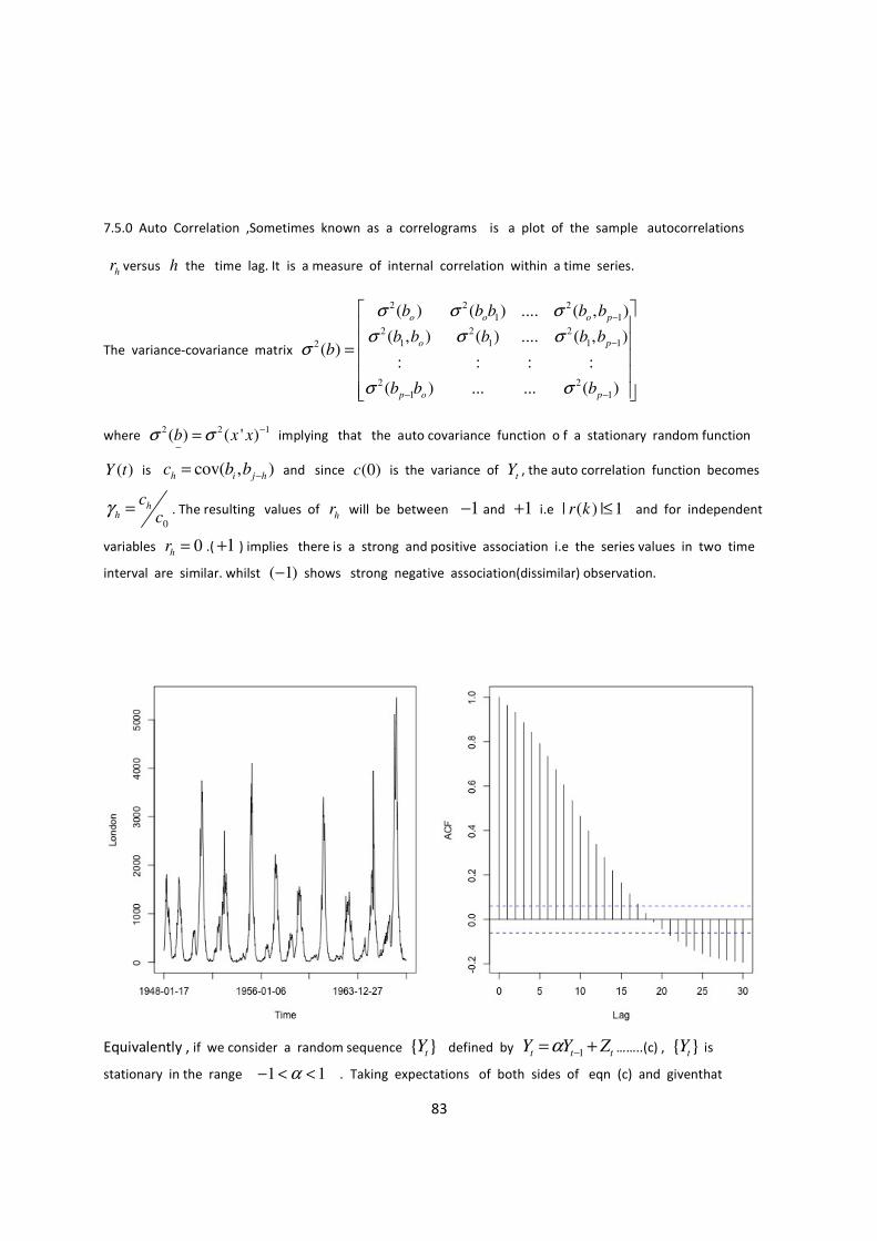
7.5.0 Auto Correlation ,Sometimes
h
r versus h the time lag. It is a m
The variance-covariance matrix σ
where 2 2 1( ) ( ' )b x xσ σ −
−= implyin
( )Y t is cov( , )h i j h
c b b −= and s
0
hh
cc
γ = . The resulting values of
variables 0h
r = .( 1+ ) implies the
interval are similar. whilst ( 1)− sh
Equivalently , if we consider a ran
stationary in the range 1 α− < <
83
es known as a correlograms is a plot of the samp
a measure of internal correlation within a time serie
2 2 2
1 1
2 2 2
1 1 1 12
2 2
1 1
( ) ( ) .... ( ,
( , ) ( ) .... ( ,( )
: : : :
( ) ... ... ( )
o o o p
o p
p o p
b b b b b
b b b b bb
b b b
σ σ σσ σ σ
σ
σ σ
−
−
− −
=
plying that the auto covariance function o f a station
d since (0)c is the variance of t
Y , the auto correlat
s of h
r will be between 1− and 1+ i.e | ( ) | 1r k ≤
there is a strong and positive association i.e the serie
shows strong negative association(dissimilar) observa
random sequence tY defined by 1t t tY Y Zα −= + …
1< . Taking expectations of both sides of eqn (c
ample autocorrelations
eries.
1
1
)
)
)
−
−
tionary random function
ation function becomes
1≤ and for independent
series values in two time
ervation.
t ……..(c) , tY is
n (c) and giventhat

( ) 0tE Z = ,we deduce that µ =
expectations and dividing by Var
...; 0,1...k
k kρ α= = then we pro
7.5.1 Estimating The Autocorrelatio
For a series , 1,......., t
Y t n= we
coefficient 1
( )(n
t
t kk
y y y
gn
= +
−=∑
plot of kγ against K is called a c
dashed horizontal lines represe
of departure from randomness
84
αµ= therefore 0µ = . Now multipliying both sides
( )t
ar Y gives 1k kρ αρ −= . Finally , 1
oρ = gives the
proceed to plot kρ against k
lation Function For Equally Spaced Series(Correlogram
we use y−
(i
y
n=∑
and define the th
k sample au
)( )t ky y
−−
− −Then the
thk sample autocorrelation coef
a correlogram of that data t
y Each correlogram
resenting the limits 2n
± , which are used for inf
ess
ides by t kY − taking
the solution
grams)
auto covariance
coefficient is k
k
o
g
gγ = ,A
am includes a pair of
r informal assessment

85
7.6.0 Wavelet;- Analysis is the analysis of the dominant frequencies in a time series
7.6.1 Introduction ;For the cosine function 1
2cos(2 0.6 )50
tX tπ π= + for 1,2,.........,500t = .
In addition normally distributed errors with mean 0 and variance 1
P=50 1
50ω = , Thus it takes 50 times(
1
50ω = ) to cycle through the cosine
function , before errors are added. The maximum and the minimum values are +2 and -2
+2
-2
0 100 200 300 400 500
If we change period to 250 and 1
0.004250
ω = =
then 1
2cos(2 0.6 )250
tX tπ π= + for 1,500t =
+2
-2
0 100 200 300 400 500

86
If the regression models becomes take s a cyclic shape
where is the randomness, the frequency and parameters estimated by
least square i.e and Suppose that we have observed at n distinct time points and
for conviniences,we assume
that n is even.our goal is to identify important frequencies in the data.To pur sue the
investigation,we consider the set of possible frequencies j
j
nω = for 1,2,....,
2
nj = ,This are
called the the harmonic frequencies.We will represent the time series as
2
1 2
1
[ ( )cos 2 ( ) ( )sin(2 ( )
n
t j j
j
j jx t t
n nβ π ω β π ω
=
= +∑ .This is a sum of sine and cosine functions
at the harmonic frequencies.Think of the 1( )j
nβ and 2( )
j
nβ as the regression parameters.
Then there are a total of n parameters because we let j move from 1 to 2
n. This means that
we have n data points and n parameters. So the fit of regressin model will be exact.The first
step in the creation of the periodogram is the estimation of the 1( )j
nβ and 2( )
j
nβ parameters
It actually not necessary to carry out regression ( ) to estimate this parameters
because Instead a mathematics device called the Fast Fourier Transform (FFT) is used.
After the parameters have been estimated we define
2 2
1 2( ) ( ) ( )j j j
pn n n
β β∧ ∧
= + .This is the sum of
squared “regression” coefficients at the frequencies j
n
1
cos( ) sin( ) ....( )m
t t
k
y t t e iiα ω β ω=
= + +∑
tz 2p
πω = ( , )θ α β=
1( ' )X X XYθ −=
1( ' )X X XYθ −=

87
7.6.2 Interpretation And Use
A relatively large value of ( )j
pn
indicates relatively more importance for the frequency j
n
(or near j
n) in explaining the oscillation in the observed series ( )
jp
n is proportional to
the squared correlation between the observed series and cosine wave with frequencies j
n.
The dorminant frequencies might be used to fit cosine( or sine) wave to the data or might
be used simply to describe the important periodicities in the series.
7.6.3 Equivalently from Fourier the series we
where and
thus we can write
parameters as and
It can be
shown that the Fourier series of with and n is odd take initial
where is the sample mean Similarly for the even n, the Fourier series
is .
Equation (ii) show we can achieve an orthogonal partitioning of more variations by
increasing and since and associated sum of squares is
1
( cos sin )2
on n
n
aa nx b nx
∞
=
+ +∑
1( )cosna f x nxdx
π
ππ −
= ∫1
( )sinnb f x kxdx
π
ππ −
= ∫
1
2 cos( )n
t
t
y t
n
ωα =
=∑
1
2 sin( )n
t
t
y t
n
ωβ =
=∑
( )f x 0ω = t ty eα= +
1,........t n= α yα−
=
( )f x x= ( 1)t t
ty eα= − + 1,......,t n=
m
( 1)t
ty
nα
−
=
∑2α

If
of the total variation in the series
The graph of against is
The figure show the spectral an
largest peak occurs at the frequ
a large peak corresponding to a
per two years
2
1
cos( )
( )
n
t
t
y t
I
ω
ω=
=∑
( )I ω ω
88
where and th
eries is
is called periodo gram.
l analysis from the first of london measles time s
frequency of 0.5 cycles/year of biennial oscillatio
to annual oscillation and also a slightly smaller one
2
1
sin( )n
t
t
y t
n
ω=
∑
0 ω π≤ ≤
ty 2
1 1
2(0) 2 ( ) ( )
n m
t
t j
jy I I I
nπ π
= =
= + +∑ ∑
d the partitioning
,
e series.The
lation. There is also
one at three cycles
)2
nj <

89
7.6.4 The Connection Between The Correlogram And The Period gram
Though the two have different rationales .The presented arguments ,show a connection
between them .For Fourier frequency ω , we can write
2 2
1 1
cos( ) sin( )
( )
n n
t t
t t
y t y t
In
ω ω
ω= =
+
=
∑ ∑2 2
1 1
( cos( ) ( )sin( )n n
t t
t t
y y t y y t
n
ω ω− −
= =
− + −
=
∑ ∑
Since
1 1
cos( ) sin( ) 0n n
t t
t tω ω= =
= =∑ ∑ . Expanding each squared term gives
2 2 2( ) ( ) cos ( ) sin ( ) ( )( ) cos( )cos( ) sin( )sin( )t t s
s t
nI y y wt t y y y y t s t sω ω ω ω ω ω− − −
≠
= − + + − − +∑ ∑∑
12
1 1
( ) 2 ( )( )cos( )n n
t t t k
k t k
y y y y y y kω−− − −
−= = +
= − + − −∑ ∑∑
Now substituting the sample auto covariance coefficients we obtain
1
1
( )2 cos( )
n
o k
ko
Ig g k
g
ωω
−
=
= + ∑ express Fourier transform as a sample of auto covariance
Finally dividing by og defines normalized period gram
1
1
( )1 2 cos( )
n
k
ko
Ik
g
ωγ ω
−
=
= + ∑ as the Fourier transform of the correlogram
7.7.0 The Spectrum Of A Stationary Random Process.
Consider a stationary random sequence cov( , )t t t kY Yγ −= .The corresponding auto covariance
generating function is ( ) ...(4)k
k
k
G Z zγ∞
=−∞
= ∑ whose arguments z ,is a complex variable .If in equation
(4). we now choose iw
z e−= where ω is thereal variable ,we obtain the spectrum of tY
,
( ) ( ) .......(5)i ik
k
k
f G e eω ωω γ
∞− −
=−∞
= = ∑ because k kγ γ −= and 2cosi ie e
ω ω ω−+ = we can write
equation (5) as 0
1
( ) 2 cos( )k
k
f kω γ γ ω∞
=
= + ∑ ,

90
revealing that spectrum isa real-valued function. If 2σ denotes the variance of tY .
we can similarly define a normalized spectrum 2
1
( )*( ) 1 2 cos( )k
k
ff k
ωω ρ ω
σ
∞
=
= = + ∑
Note; The normalized spectrum bears the same relationship to the autocorrelation
function as does the spectrum to the auto covariance and any non-negative valued function ( )f ω
on ( (0, )π defines a legitimate spectrum.
7.7.1 Example
A first – order autoregressive process. Suppose that tY is defined by 1t t tY Y Zα −= + where tZ
is a randomized sequence and 1 1α− < < we have already seen that the autocorrelation function tY is
; 0,1,.......,k
k kρ α= = Thus the normalized spectrum of tY is *( )ik
k
k
f eωω ρ
∞−
=−∞
= ∑ It can be shown
that 12 2*( ) (1 ) 1 2 cos( ) .......(6)f ω α α ω α
−= − − + Normalized spectrum for each of 0.5,0.5α = −
and 0.9 Note For negative , *( )fα ω is an increasing function of ω

91
7.7.3 Discrete And Continuous Spectrum
Spectrum plots gives information about how power (or variance) in a series
is distributed according to frequencies.For auto covariance cov ,h t t hc Y Y −= and auto covariance
function ish
h
h
c z∞
=−∞∑ and since
h hc c−= and 2cos( )i ie eω ω ω−+ = we write a spectrum real
valued
1
( ) 2 cos( )o k
h
f c hω γ ω∞
=
= + ∑ Conversion of time-indexed data into estimates of autocorrelation
or spectrum depends partly on Fourier transformation of ( )c τ to obtain ( )F A .If Continuous component is
missing i.e ( )f λ =0 for all λ . the time spectrum is said to have a discrete spectrum (point spectrum).
( ) ( )i k
k
k
C e pλ ττ λ
∞
=−∞
= ∑ moreover ( ) (0)k
k
p Cλ∞
=−∞
= < ∞∑
Thus since summable series are square summable 2( )k
k
p λ∞
=−∞
< ∞∑ . It follows that the
spectrum function can be obtained from auto covariance by the expression
1( ) lim ( )
2k
T
i
kt
T
p C e dλ τλ τ τ−
→∞−
= ∫ ,expression yields ( )p λ for all λ and ( )dF A can be
obtained. For continuous spectrum ( ) ( )iC e f d
λττ λ λ∞
−∞
= ∫ is valid and ( ) (0)f d Cλ λ∞
−∞
= < ∞∫
The auto covariance and spectrum of an almost periodic function
Let i t
j
j
Xt C eλ
∞
=−∞
= ∑ be an almost periodic function with 2| |j
j
C∞
=−∞
< ∞∑
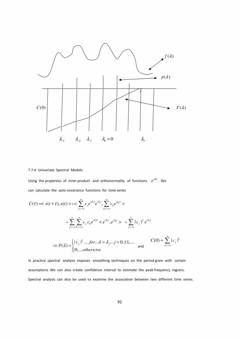
92
( )f λ
( )p λ
(0)C ( )F λ
3λ− 2λ− 1λ− 0 0λ = 3λ
7.7.4 Univariate Spectral Models
Using the properties of inner product and orthonormality of functions i it
eλ
. We
can calculate the auto covariance functions for time series
( ) ( ), ( )C x t x tτ τ=< + > = ,j j ki i t i
j k
j k
c e e c eλ τ λ λ τ
∞ ∞
=−∞ =−∞
< >∑ ∑
= ,j j ki k i t i t
j k
j k
c c e e eλ λ λ
∞ ∞ −
=−∞ =−∞
< >∑ ∑ =2| | ji t
j
j
c eλ
∞
=−∞∑
2| | .... ... ... 0, 1,....( )
0;....
j jc for j
Potherwise
λ λλ
= = ±⇒ =
and
2(0) | |j
j
C c∞
=−∞
= ∑
In practice spectral analysis imposes smoothing techniques on the period gram with certain
assumptions .We can also create confidence interval to estimate the peak frequency regions.
Spectral analysis can also be used to examine the association between two different time series.

93
RECOMMEDATION
To show further application of lebesgue integration in
(i)n
R -spaces and stokes and green theorems.
(ii) Statistical methods such discrete
and continuous solutions of expectations
(iii)In Time Series Analysis Solutions
94
CONCLUSION
This study describes the Extensions of Riemann theory of integrations, first to Riemann
Stieltjes integration, then to the most notable extensions, ’The Lebesgue Theory Of Integration.
As a result we are able to solve the discontinuous functions, such as step-functions, recover f(t) from
F’(t),and calculate areas covered by continuous functions with increased limits e.g Rn spaces.
95
REFERENCES
1.Burkill.J.C”The lebesgue Integral”, Cambridge press, New York,1951.
2.Rudin.W”Real and Complex Analysis”,2d Edition ,Mcgraw-Hill Book Company, New York,1974.
3.Herstein,I.N.”Topics in Algebra”, Blaisdell Publishing Company, New York,1964.
4.Artin .E.”The Gamma Function” ,Holt, Rinehart and wiston ,Inc, New York,1964.

96