Extensible Data SkippingPaula Ta-Shma, Guy Khazma, Gal Lushi, Oshrit Feder

IBM ResearchEmail: {paula,oshritf}@il.ibm.com, {Guy.Khazma,Gal.Lushi}@ibm.com

Abstract—Data skipping reduces I/O for SQL queries byskipping over irrelevant data objects (files) based on theirmetadata. We extend this notion by allowing developers todefine their own data skipping metadata types and indexesusing a flexible API. Our framework is the first to nativelysupport data skipping for arbitrary data types (e.g. geospatial,logs) and queries with User Defined Functions (UDFs). Weintegrated our framework with Apache Spark and it is nowdeployed across multiple products/services at IBM. We presentour extensible data skipping APIs, discuss index design, andimplement various metadata indexes, requiring only around 30lines of additional code per index. In particular we implementdata skipping for a third party library with geospatial UDFsand demonstrate speedups of two orders of magnitude. Ourcentralized metadata approach provides a x3.6 speed up evenwhen compared to queries which are rewritten to exploit Parquetmin/max metadata. We demonstrate that extensible data skippingis applicable to broad class of applications, where user definedindexes achieve significant speedups and cost savings with verylow development cost.

I. INTRODUCTION

According to today’s best practices, cloud compute and stor-age services should be deployed and managed independently.This means that potentially huge datasets need to be shippedfrom the storage service to the compute service to analysethe data. This is problematic even when they are connectedby a fast network, and highly exacerbated when connectedacross the WAN e.g. in hybrid cloud scenarios. To addressthis, minimizing the amount of data sent across the networkis critical to achieve good performance and low cost. Dataskipping is a technique which achieves this for SQL analyticson structured data.

Data skipping stores summary metadata for each object(or file) in a dataset. For each column in the object, thesummary might include minimum and maximum values, alist or bloom filter of the appearing values, or other metadatawhich succinctly represents the data in that column. Thismetadata can then be indexed to support efficient retrieval,although since it can be orders of magnitude smaller than thedata itself, this step may not be essential. The metadata canbe used during query evaluation to skip over objects whichhave no relevant data. False positives for object relevance areacceptable since the query execution engine will ultimatelyfilter the data at the row level. However false negatives mustbe avoided to ensure correctness of query results.

Unlike fully inverted database indexes, data skipping in-dexes are much smaller than the data itself. This property iscritical in the cloud, since otherwise a full index scan couldincrease the amount of data sent across the network instead of

reducing it. In the context of database systems, data skipping isused as an additional technique which complements classicalindexes. It is referred to as synopsis in DB2 [41] and zonemaps in Oracle [48], where in both cases it is limited tomin/max metadata. Data skipping and the associated topicof data layout, has been addressed in recent research papers[44], [42] and is also used in cloud analytics platforms [12],[6]. Data skipping metadata is also included in specific dataformats [5], [4].

Despite the important role of data skipping, almost allproduction ready implementations are limited to min/maxindexes over numeric or string columns, with the exceptionof the ORC/Parquet formats which also support bloom filters.Moreover, queries with UDFs cannot be handled. For example,today’s implementations do not support data skipping for thequery below1.

SELECT max(temp) FROM weatherWHERE ST_CONTAINS(India, lat, lon)AND city LIKE ’%Pur’

We address this by implementing data skipping support forApache Spark SQL[21], and making it extensible in severalways.

1) users can define their own data skipping metadata beyondmin/max values and bloom filters

2) data skipping can be applied to additional column typesbeyond numeric and string types e.g. images, arrays, userdefined types (UDTs), without changing the source data

3) users can enable data skipping for queries with UDFs bymapping them to conditions over data skipping metadata

For the query above, our framework allows defining a suffixindex for text columns and mapping the LIKE predicate toexploit it for skipping, as well as mapping the ST_CONTAINSUDF to min/max metadata on geospatial attributes. This canreduce the amount of data scanned by orders of magnitude.Our implementation supports plugging in metadata stores,with connectors for Parquet and Elastic Search, and is in-tegrated into multiple IBM products/services including IBMCloud®SQL Query, IBM Analytics Engine and IBM CloudPak®for Data [12], [10], [11].

We demonstrate various use cases for extensible data skip-ping, show its benefits far outweigh its costs, and show thatcentralized metadata storage provides significant performancebenefits beyond relying on data (Parquet/ORC) formats onlyfor data skipping.

1’India’ denotes a polygon with India’s geospatial coordinates

arX

iv:2

009.

0815

0v2

[cs

.DB

] 1

5 N

ov 2

020

Fig. 1: Index creation flow

This paper is organised as follows. Section II covers ex-tensible data skipping APIs, section III discusses our imple-mentation, section IV covers metadata index design, section Vdiscusses experimental results, section VI covers related workand section VII presents our conclusions.

II. EXTENSIBLE DATA SKIPPING

Our Scala APIs allow the developer to (1) create dataskipping indexes, including adding support for new indextypes, and (2) specify how to exploit data skipping indexesduring query evaluation by mapping predicates to operationson summary metadata. Our framework covers compositions ofpredicates e.g. using AND, OR and NOT, allowing expressionsof arbitrary complexity.

A. Extensible Data Skipping APIs

For simplicity, we provide a running example formin/max data skipping, but our APIs can handle ar-bitrary predicates/UDFs and user defined metadata (e.g.LIKE/ST_CONTAINS and suffix indexes). Useful data skip-ping metadata for the query below is the minimum andmaximum temperature for an object (data subset2).

SELECT * FROM weather WHERE temp > 101

1) Index Creation: Users can define new metadata typeswhich extend our MetaDataType class, such as the examplebelow.

abstract class MetadataTypecase class MinMaxMetaData(col: String,

var min: Double, var max: Double)extends MetadataType

Indexes are created explicitly and executed as a dedicatedSpark job. Index creation runs in 2 phases - see figure 1. Thefirst phase accepts a Spark DataFrame (representing an object)and generates metadata having some MetaDataType. Thesecond phase translates this metadata to a metadata storerepresentation. In order to implement the first phase, thedeveloper extends the Index class.

abstract class Index(params: Map[String,String], col: String*) {

def collectMetaData(df: DataFrame):MetadataType

}

Our example MinMaxIndex extends Index, andcollectMetadata returns a MinMaxMetaData instancecontaining minimum and maximum values for the givenobject column.

2Other alternatives for data subsets are blocks, row groups etc. Ourintegration with Spark skips at the object level.

Fig. 2: An Expression Tree (ET) for the example query

Fig. 3: Query evaluation flow

2) Query Evaluation: Spark has an extensible query opti-mizer called Catalyst[21], which contains a library for repre-senting query trees and applying rules to manipulate them. Wefocus on query predicates i.e. boolean valued expressions typi-cally appearing in a WHERE clause, which can be representedas Expression Trees (ETs). Figure 2 shows the expression treefor our example query.

We analyse ETs and label tree nodes with Clauses. A Clauseis a boolean condition that can be applied to a data subset s,typically by inspecting its metadata. Note that for a queryET e, for every vertex v in e, we denote the set of Clausesassociated with v by CS(v).

Definition 1. Denote the universe of possible data subsets(i.e., objects) by U . A Clause c is a boolean function U →{0, 1}.

Definition 2. For a Clause c and a (boolean) query expressione, we say that c represents e (denoted by c o e), if for everydata subset S, whenever there exists a row r ∈ S that satisfiese, then S satisfies c.

This means that if S does not satisfy c, then S can besafely skipped when evaluating the query expression e. Forexample, let e be temp > 101. Given a data subset S, let cbe the Clause maxr∈S temp(r) > 101. Then c represents e.Therefore, objects wheremaxr∈S temp(r) <= 101 can be safely skipped.

Query evaluation is done in 2 phases as shown in figure 3. Inthe first phase, a query’s ET e is labelled using a set of clausesand the clauses are combined to provide a single clause whichrepresents e. The labelling process is extensible, allowing fornew index types and for new ways of using metadata. In thesecond phase, this clause is translated to a form that can beapplied at the metadata store to filter out the set of objectswhich can be skipped during query evaluation.

The labelling process is done using filters. Typically therewill be one or more filters for each metadata index type. Forexample, we will define a MinMaxFilter to correspond toour MinMaxIndex.

Definition 3. An algorithm A is a filter if it performs thefollowing action: When given an expression tree e as input,for every (boolean valued) vertex v in e, it adds a set of clauses

Fig. 4: The result of a filter on an ET

C s.t. ∀c ∈ C: c o v to the existing set of clauses. 3

For example a filter f might label our ET usingMaxClause, as shown in figure 4, where for a column name cand a value v, MaxClause(c,>,v) is defined as maxr∈S c(r) >v. Since MaxClause(temperature,>,101) represents the node towhich it was applied, f acted as a filter. Since maxr∈S c(r)is stored as metadata in MinMaxMetaData, MaxClause canbe evaluated using this metadata only.

We provide the user with APIs to define clauses and filters.A Clause is a trait which can be extended. A Filter needsto define the labelNode method.

case class MaxClause(col:String, op:opType,value:Literal) extends Clause

case class MaxFilter(col:String) extendsBaseMetadataFilter {

def labelNode(node:LabelledExpressionTree):Option[Clause] = {

node.expr match {case GreaterThan(attr: Attribute, v:

Literal) if attr.name == col =>Some(MaxClause(col, GT, v))

case _ => None}}

Filters typically use pattern matching on the ET structure4.Similarly we can define a MinFilter which can label a treewith MinClauses. Patterns can also match against UDFs inexpression trees e.g. ST_CONTAINS - see also section V-Cfor queries using UDFs.

In some cases a filter’s patterns may need to match againstcomplex predicates using AND/OR/NOT. For example, theGeoBox index (section IV) stores a 2 dimensional boundingbox for each object and the corresponding filter needs to matchagainst an AND with child constraints on both lat and lng.Figure 5 illustrates this.

Each MetaDataFilter needs to be registered in oursystem, and during query optimization we inspect the typesof metadata that were collected and run the relevant filterson the query’s ET. Running the complete set of registeredfilters will generate an ET where each node can be labelledby multiple Clauses. For every vertex v in e, we denote theset of Clauses associated with v by CS(v). We recursivelymerge all of an ET’s Clauses to form a unified Clause whichrepresents it. This Clause is then applied to the metadata to

3Note that for a particular node, a filter might not add any clauses (this isthe special case of adding the empty set).

4For simplicity we left out the cases of ≤ and ≥ for MaxFilter above.

Fig. 5: The result of a geobox filter on a complex queryexpression

Fig. 6: Modified Spark query execution flow after integrationwith extensible data skipping

make a final skipping decision. For a full formal description ofthe algorithm used and proof of correctness, see Appendix A

III. IMPLEMENTATION

We implemented data skipping support for Apache SparkSQL[21] as an add-on Scala library which can be added tothe classpath and used in Spark applications. Our work appliesto storage systems which implement the Hadoop FileSystemAPI, which includes various object storage systems as well asHDFS. We tested our work using IBM Cloud Object Storage(COS) and the Stocator connector [19], [46]. Metadata isstored via a pluggable API which we describe in sectionIII-B. The library supports multiple levels of extensibility:code which implements any of our extensible APIs such asmetadata types, and clause and filter definitions, as well asadditional metadata stores, can be added as plugin libraries.

A. Spark Integration

Spark uses a partition pruning technique to filter the list ofobjects to be read if the dataset is appropriately partitioned.Our approach further prunes this list according to data skippingmetadata as shown in figure 6.

Our technique applies to all Spark supported native for-mats e.g. JSON, CSV, Avro, Parquet, ORC, and can benefitfrom optimizations built into those formats in Spark. Unlikeapproaches which embed data skipping metadata inside thedata format which require reading footers of every object, ourapproach avoids touching irrelevant objects altogether. It alsoavoids wasteful resource allocation because when relying ona format’s data skipping, Spark allocates resources to handleentire objects, even when only object footers need to beprocessed. We provide an API for users to retrieve how muchdata was skipped for each query.

We used APIs provided by Spark’s Catalyst query optimizerto achieve this without changing core Spark. In particular,we added a new optimization rule using the Spark sessionextensions API[34]. Spark SQL maintains anInMemoryFileIndex which tracks the objects to be readfor the current query and their properties. Our rule wrapsthe InMemoryFileIndex with a new class extending it byadding the additional filtering step from figure 6.

We refrain from skipping objects when our metadata aboutthem is stale. This can happen if objects are added, deletedor overwritten in a dataset after indexing it. We keep track offreshness using last modified timestamps, which are retrievedduring file listing by the InMemoryFileIndex. We alsoprovide a refresh operation, which updates stale metadata.

B. Metadata Stores

We support a pluggable API for metadata stores includingthe specification of how metadata and clauses should betranslated for a particular store. This includes the indexingtime translation API for figure 1 and the query time translationAPI for figure 3. The key property is that these translationsshould preserve the correctness of our skipping algorithm. Weused this API to implement both Parquet and Elastic Search[8]metadata stores.

It is now widely accepted practice to use the same storagesystem for both data and metadata[7], [3], [2], avoidingdeployment of an additional metadata service. This is achievedusing our Parquet metadata store, and all storage systemsimplementing the Hadoop FS API are supported. Relevantmetadata indexes are scanned prior to query execution, butthis cost is not significant, since metadata is typically con-siderably smaller than data. By leveraging Parquet’s column-wise compression and projection pushdown for metadata, weminimize the amount of metadata that needs to be read perquery, ensuring low overhead. Use of Parquet also allowsgenerating and storing metadata for multiple columns together,resulting in better indexing and refresh performance, comparedwith storing indexes on each column separately.

C. Protecting Sensitive Data and Metadata

Security and privacy protection for sensitive data are es-sential for today’s cloud services. Parquet supports column-wise encryption of sensitive columns in a modular and effi-cient fashion[16], [17], and being format-agnostic, our librarysupports skipping over encrypted parquet data transparently.However, an end-to-end solution needs to encrypt metadata,since it can also leak sensitive information. To prevent leakage,when storing metadata in Parquet, we implemented an optionto encrypt indexes on sensitive columns, by assigning a key toeach index. A user can choose the same key used to encryptthe column the index originates from, choose another key, orleave the index as plaintext. This scheme enables scenariossuch as storing data and metadata at a shared location, whereeach user can only access a subset of the columns and indexesaccording to their keys.

Spark’s partition pruning capability relies on either (1) awidely accepted naming convention which names appropri-ately partitioned data objects according to their partitioningcolumn name and column value or (2) a Hive metastore. Thefirst option leaks metadata into object names, and thereforepartitioning according to sensitive columns is problematic. Useof a Hive metastore in a multi-tenant cloud service pushesthe problem of managing sensitive multi-tenant metadata tothe underlying database. An alternative is to rely on our dataskipping framework for partition pruning, thereby ensuringend-to-end data and metadata protection, without sacrificingperformance.

IV. METADATA INDEX DESIGN

In this section we explain the requirements of a good meta-data index type and cover indicators of skipping effectiveness.We show that in theory both selecting and designing optimalindexes are hard problems. However, we demonstrate practicalchoices that work well in this and the following section. Wesurvey various index types implemented using our APIs witha summary in table I.

Our goal is to minimize the total number of bytes scanned,because there is a close correlation between this and querycompletion time (e.g. see section V). Moreover, users ofserverless SQL services are typically billed in proportion tothe number of bytes scanned[1], [13].

For each query, prior to reading the data, the relevantmetadata is scanned and analyzed. As long as the metadatais much smaller than the data, this approach can significantlyreduce the amount of data scanned overall. For big datasetsthe overhead of scanning metadata is usually insignificantcompared to the benefits of skipping data (see figure 8), andin some cases metadata can also be cached in memory oron SSDs. When using our Parquet metadata store, we readonly the relevant metadata indexes by using Spark and Parquetcolumn projection capabilities.

A. Indicators of Skipping Effectiveness

Given a dataset (set of rows) D and a query Q, a row r inD is relevant to Q if r must be read in order to compute Qon D. Let Dr denote the set of relevant rows in D. AssumingD is stored as objects5, let O denote the set of all objects forD, let Or denote the set of objects relevant to Q (i.e. havingat least one relevant row), and let Om be the set of objectsdeemed relevant according to the metadata associated with D.Note that Or ⊆ Om. Note that Os = O − Om is the set ofobjects that can be skipped.

Denote the number of rows in object o (or dataset D) as |o|(|D|). All definitions below are w.r.t. a dataset D and a queryQ.

Definition 4. The selectivity σ of a query is the proportionof relevant rows σ = |Dr|

|D|

5alternatively other units can be considered such as blocks, row groups etc.

Data skipping can potentially reduce bytes scanned forselective6 queries. The definitions use relevant rows rather thanrows in the result set to account for queries which performfurther computations such as aggregation.

Definition 5. The layout factor λ of a query is the proportionof relevant rows in relevant objectsλ = |Dr|∑

o∈Or|o|

Mixing relevant and irrelevant rows in the same objectdecreases the layout factor. A high layout factor (grouping rel-evant rows together) increases the potential for data skipping.To realise this potential we need effective metadata.

Definition 6. The metadata factor µ of a query isµ =

∑o∈Or

|o|∑o∈Om

|o|

The metadata factor is closely related to the metadata’sfalse positive ratio - a low false positive ratio gives rise toa high metadata factor. In addition the metadata factor takesinto account the relative size of each object. A high metadatafactor denotes that the metadata is close to optimal given thedata layout.

Definition 7. The scanning factor ψ of a query is theproportion of rows actually scanned (using metadata)ψ =

∑o∈Om

|o||D|

Our aim is to achieve the lowest possible scanning factor.According to our definitions

ψ =σ

λµ(1)

To achieve this for a selective query we need λµ to be high,and we are equally dependent on good layout and effectivemetadata7.

We focus here on metadata effectiveness for any given datalayout, and refer the reader to previous work regarding datalayout optimization[44], [42]. In practice, often data layoutis given and cannot be changed e.g. legacy requirements,compliance, encryption of one or more sensitive columns. Inother cases, re-layout of the data is too costly, or it might bedifficult to meet the needs of multiple conflicting workloadswithout duplicating the entire dataset.

Our approach is to enable an extensible range of metadatatypes, which cater to data within a reasonable range oflayout factors. Generating data skipping metadata is typicallysignificantly cheaper than changing the data layout, since noshuffling of the data is needed. Moreover, unlike data layout,it can be done without write access to the dataset and onlyrequires read access to the column(s) at hand. Each user canpotentially store metadata corresponding to their particularworkload.

On the other hand, using equation 1, we can identify caseswhere the layout factor is prohibitively low and good skippingis unachievable without re-layout.

6Selectivity ranges between 0 and 1.“Highly selective” queries have closeto 0 selectivity

7Note that the scanning factor is not defined for queries with 0 selectivity

To take averages of skipping indicators when consideringmultiple queries, we use the geometric mean, following[22].Let G(X) denote (

∏ni=1 xi)

1n . Given a dataset D and a

workload with queries q1, . . . , qn, where for each qi we haveψi = σi

λiµi, then we also have

G(ψ) =G(σ)

G(λ)G(µ)(2)

We apply this approach to measuring the skipping indicatorson real world datasets and workloads in section V.

B. The Index Selection Optimization Problem

Given a dataset D and query workload (set of queries) Q,it is natural to ask what is the optimal set of metadata indexeswe can store to achieve the lowest possible scanning factor.Since the workload and data layout are given, σ and λ aregiven, and to achieve low ψ we need to achieve high µ. Weassume that every metadata index i has a cost ci, and that weneed to stay within a given metadata budget K. A natural costdefinition is the size of the metadata in object storage. We alsoassume that each index i ∈ I provides a benefit vi which in ourcase corresponds to the increase in µ as a result of i. Ideally,given K and a set of candidate metadata indexes I , one couldchoose an optimal subset I ′ ⊆ I which gives maximal µ whilestaying within budget. We show that this problem is NP-hardusing a reduction from the knapsack problem. Previous workshowed that the problem of finding a data layout providingoptimal skipping is also NP-hard[44].

Problem 8. Given dataset D, workload Q, a set of indexes I ,and a metadata budget K, find I ′ ⊆ I that maximizes

∑i∈I′ vi

subject to∑i∈I′ ci ≤ K.

Claim 9. Problem 8 is NP-hard.

Proof. By reduction from {0,1}-knapsack. Knapsack itemweight and value correspond to the cost and benefit of anindex respectively, and knapsack capacity corresponds to themetadata budget. Clearly, maximizing the value of items in theknapsack within capacity is equivalent to maximizing indexbenefit within a metadata budget.

Remark 10. This formulation shows that even in the specialcase where the benefit of an index is independent from otherindexes, the problem is hard. In the general case, the benefit ofindexes is relative since, for example, an index which achievesmaximal µ renders further addition of indexes obsolete.

Given a fixed metadata budget, choosing optimal indexes isa hard problem. However, for many index types8 we store afixed #bytes per object, thereby bounding the index size to asmall fraction of the data size. Using such index types, it isreasonable to index all data columns, assuming the metadatais stored in the same storage system as the data (i.e. with thesame storage/access cost).

8all index types in table I except for value list and prefix/suffix indexes

C. An Index Design Optimization Problem

Choosing an optimal set of indexes is hard. What aboutdesigning a single optimal index? We show that this is hardeven for a range query workload on a single column. Considera single column c with a linear order e.g. integers, and aworkload Q with range queries over c i.e. queries of theform

SELECT * FROM DWHERE c between c1 and c2

Storing min/max metadata only for c may not achieve maximalµ, for example, when an object’s rows have gaps in columnc between the min and max values. In this case if c1 and c2both fit inside the gap then min/max metadata will give a falsepositive for the query above. A gap list metadata index couldstore a list of such gaps per object, and be used to skip objectshaving gaps covering the intervals used in queries. Given adataset D, a workload Q and metadata budget of k gaps, whichgaps should be stored to give optimal µ? (We assume the costof each gap is equal). An algorithm which achieves this isprovided in [31]. However, we show that allowing queries withdisjunction turns this into a hard problem.

Problem 11. Given a dataset D with a column c having alinear order, a workload Q comprising of disjunctive rangequeries over c, and a metadata budget of K gaps, find a setof k gaps where k ≤ K such that µ is maximized.

Problem 12. (Densest k-Subhypergraph problem) Given ahypergraph G = (V,E) and a parameter k, find a set of kvertices with maximum number of hyperedges in the subgraphinduced by this set[29].

Claim 13. Problem 11 is NP-hard.

Proof. By reduction from the densest k-Subhypergraph prob-lem. Given G = (V,E) and k, we construct an input toproblem 11 as follows. We create a dataset with one objectO such that its column c induces |V | gaps - {g1, g2, .., g|V |},and use the function f(vi) = gi to map each vertex to a gap.Each hyperedge e ∈ E is mapped to a query with a WHEREclause comprised of a predicate of the form: ∨v∈ec ∈ f(v).In order to skip O for this query we need exactly those gapsin {f(v)|v ∈ e}. In this setting maximizing µ (the numberof queries where O is skipped) is equivalent to finding thedensest k-Subhypergraph.

D. Metadata Index Types

Table I contains a summary of common index types (Min-Max, BloomFilter) as well as novel ones we found usefulfor our use cases and implemented for our Parquet metadatastore. All metadata enjoys Parquet columnar compression andefficient encoding - therefore the Bytes/Object values in thetable can be considered an upper bound.

The MetricDist index enables similarity search queriesusing UDFs based on any metric distance e.g. Euclidean,Manhattan, Levenshtein. Applications include document andgenetic similarity queries. Recently semantic similarity queries

have been applied to databases[26], where values are con-sidered similar based on their context, allowing queries suchas “which employee is most similar to Mary?”. Assuming ametric function for similarity, extensible data skipping can besuccessfully applied.

Additional index types can be easily integrated by imple-menting our APIs - example candidates include SuRF[47],HOT[24], HTM[45]. Recent work demonstrated the use ofrange sets (similar to our gap lists) to optimize queries withJOINs[35]. Adding a new index type via our APIs requiresroughly 30 lines of new code.

E. A Hybrid Index

When a column typically has low cardinality per object, avalue list is both more space efficient than a bloom filter andavoids false positives. However, for high cardinality, value listmetadata size can approach that of the data. In order to achievethe best of both worlds, we implemented a hybrid index, whichuses a value list up to a certain cardinality threshold, and abloom filter otherwise. We now explain how we determinedan appropriate threshold.

Assuming equality predicates only, we compare value listand bloom filter indexes using the formulas presented in tableI. Our aim is to minimize the total bytes scanned for dataand metadata. Given an object of size |o|, a column with vdistinct values each one of size b bits, and a workload Q ={qi}ni=1 of exact match queries, let Ei ∈ {0, 1} be the eventin which o must be read for qi. It follows that the average datato be scanned for the workload using a bloom filter index isapproximately 1

n

∑ni=1(−v ln f

ln2 2+ Ei|o| + (1 − Ei)f |o|). The

average data to be scanned for the workload using value listis exactly 1

n

∑ni=1(vb + Ei|o|). Therefore, a value list index

is preferable when:

v(b+ln f

ln2 2) < f |o|(1− 1

n

n∑i=1

Ei)

The term 1n

∑ni=1Ei can be approximated using the expected

scanning factor when using a value list index, which can bederived from the workload mean layout and selectivity factorsusing equation 2.

For example, given an object of size 64MB with a stringcolumn of up to 64 characters (b = 512) and a target scanningfactor of 0.01, a value list up to 10,088 elements is preferableover a bloom filter with f = 0.01. We implemented a hybridindex which creates a bloom filter or value list per objectaccording to the column cardinality. By default we use athreshold of 10K elements based on the above example, butthis threshold can be changed according to dataset properties.

V. EXPERIMENTAL RESULTS

We focus on use cases where data is born in the cloudat a high, often accelerating, rate so highly scalable and lowcost solutions are critical. We demonstrate our library forgeospatial analytics (representing IoT workloads in general)and log analytics on 3 proprietary datasets. We collect skippingeffectiveness indicators and discuss their effect on the scanning

TABLE I: Data Skipping Index Types

Index Type Description Column Types Handles Predicates1 Bytes/Object2

MinMax Stores minimum/maximum values for a column ordered p(n, c) 2bGapList Stores a set of k gaps indicating ranges where there are ordered p(n, c) kb

no data points in an objectGeoBox Applies to geospatial column types e.g. Polygon, Point. geospatial geo UDFs 2xb

Stores a set of x bounding boxes covering data pointsBloomFilter Bloom filter is a well known technique[25] hashable n = c, n ∈ C −v ln f

ln2 2(in bits)

ValueList Stores the list of unique values for the column has =, text n = c, n ∈ C, LIKE vbPrefix Stores a list of the unique prefixes having b1 characters text LIKE ’pattern%’ v1b1Suffix Stores a list of the unique suffixes having b2 characters text LIKE ’%pattern’ v2b2

Formatted Handles formatted strings. There are many uses cases. text template based UDFs variesMetricDist Stores an origin, max and min distance per object has metric dist metric distance UDFs 2m+ b

1 p ∈ {<,≤, >,≥,=}. n is a column name and c is a literal, C is a set of literals.2 b is the (average) number of bytes needed to store a single column element. v is the number of distinct values in a column for the

given object. k is the number of gaps (configurable). x is the number of boxes per object. v1 (v2) is the number of distinct valueswith prefix (suffix) of size b1 (b2). m is the number of bytes needed to store a distance value. f is the false positive rate (f ∈ (0, 1)).

factor (hence data scanned). All experiments were conductedusing Spark 2.3.2 on a 3 node IBM Analytics Engine cluster,each with 128GB of RAM, 32 vCPU, except where mentionedotherwise. The datasets are stored in IBM COS. All experi-ments are run with cold caches.

A proprietary (1) Weather Dataset contains a 4K grid ofhourly weather measurements. The data consists of a singletable with 33 columns such as latitude, longitude, temperatureand wind speed. The data was geospatially partitioned usinga KD-Tree partitioner[42]. One month of weather data wasstored in 8192 Parquet objects using snappy compression witha total size of 191GB.

The two proprietary http server log datasets below aresamples of much larger datasets and use Parquet with snappycompression:

(2) A Cloud Database Logs dataset, consisting of a singletable with 62 columns such as db name, account name,http request. The data was partitioned daily with layout ac-cording to the account name for each day, resulting in 4Kobjects with a total size of 682GB.

(3) A Cloud Storage Logs dataset, consisting of a singletable with 99 columns such as container name, account name,user agent. The data was partitioned hourly, resulting in 46Kobjects with a total size of 2.47TB.

A. Indexing

Use of our APIs allows adding new index types achievingsimilar performance to native index types with little pro-grammer effort. Table II in appendix B reports statistics forindexing a single column using various index types on ourdatasets. In addition, we implemented an optimization whichreads min/max statistics from Parquet footers, which givessignificant speedups when only MinMax indexes are used onParquet data9.

Figure 7 shows that indexing multiple columns using theHybrid index is significantly faster than indexing each columnseparately10, even for Parquet data where columns are scanned

9If additional index types are used it provides no benefit since the Parquetrow groups need to be accessed in any case.

10other index types behave similarly

Fig. 7: Indexing time/size vs #columns (log scale) with Hybrid(cloud database logs) and MinMax (weather)

individually. For MinMax the indexing time remains low(benefiting from our MinMax optimization) and flat whenvarying the number of columns.

We note that indexing can be done per object at datageneration or ingestion time, and can alternatively be doneusing highly scalable serverless cloud frameworks e.g. [33].

B. Metadata versus Data Processing

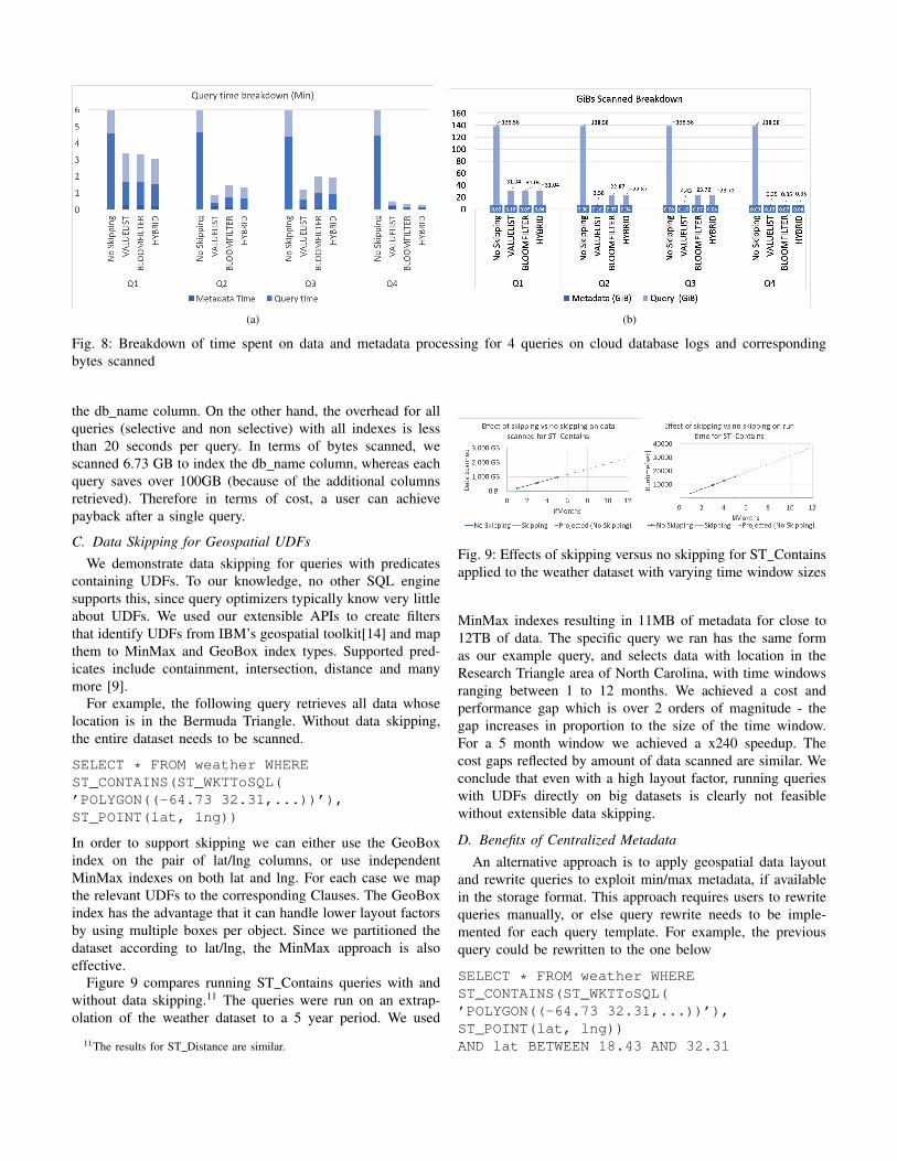
Figure 8 shows time and bytes scanned for 4 queriessearching for different values of the db name column (clouddatabase logs dataset). The queries retrieve 8 columns, andwe compare ValueList, BloomFilter and Hybrid indexes onthe db name column, and in all cases either ValueList or theHybrid index outperforms BloomFilter (whereas BloomFilteris the index most widely adopted in practice). There is a clearcorrespondence between bytes scanned and query completiontimes, and data skipping reduces query times roughly betweenx3 and x20. In all cases, the time spent on metadata processingis a small fraction of the overall time. For all queries, theHybrid index requires the least metadata processing timebecause of its smaller size. For Q4, when almost all data isskipped, the Hybrid index is superior for this reason. For Q2and Q3, Hybrid and BloomFilter incur false positives and soretrieve more data than ValueList, resulting in longer querytimes.

We point out that for this scenario it only takes around3 queries to save the 10 mins that were spent on indexing

(a) (b)

Fig. 8: Breakdown of time spent on data and metadata processing for 4 queries on cloud database logs and correspondingbytes scanned

the db name column. On the other hand, the overhead for allqueries (selective and non selective) with all indexes is lessthan 20 seconds per query. In terms of bytes scanned, wescanned 6.73 GB to index the db name column, whereas eachquery saves over 100GB (because of the additional columnsretrieved). Therefore in terms of cost, a user can achievepayback after a single query.

C. Data Skipping for Geospatial UDFs

We demonstrate data skipping for queries with predicatescontaining UDFs. To our knowledge, no other SQL enginesupports this, since query optimizers typically know very littleabout UDFs. We used our extensible APIs to create filtersthat identify UDFs from IBM’s geospatial toolkit[14] and mapthem to MinMax and GeoBox index types. Supported pred-icates include containment, intersection, distance and manymore [9].

For example, the following query retrieves all data whoselocation is in the Bermuda Triangle. Without data skipping,the entire dataset needs to be scanned.

SELECT * FROM weather WHEREST_CONTAINS(ST_WKTToSQL(’POLYGON((-64.73 32.31,...))’),ST_POINT(lat, lng))

In order to support skipping we can either use the GeoBoxindex on the pair of lat/lng columns, or use independentMinMax indexes on both lat and lng. For each case we mapthe relevant UDFs to the corresponding Clauses. The GeoBoxindex has the advantage that it can handle lower layout factorsby using multiple boxes per object. Since we partitioned thedataset according to lat/lng, the MinMax approach is alsoeffective.

Figure 9 compares running ST Contains queries with andwithout data skipping.11 The queries were run on an extrap-olation of the weather dataset to a 5 year period. We used

11The results for ST Distance are similar.

Fig. 9: Effects of skipping versus no skipping for ST Containsapplied to the weather dataset with varying time window sizes

MinMax indexes resulting in 11MB of metadata for close to12TB of data. The specific query we ran has the same formas our example query, and selects data with location in theResearch Triangle area of North Carolina, with time windowsranging between 1 to 12 months. We achieved a cost andperformance gap which is over 2 orders of magnitude - thegap increases in proportion to the size of the time window.For a 5 month window we achieved a x240 speedup. Thecost gaps reflected by amount of data scanned are similar. Weconclude that even with a high layout factor, running querieswith UDFs directly on big datasets is clearly not feasiblewithout extensible data skipping.

D. Benefits of Centralized Metadata

An alternative approach is to apply geospatial data layoutand rewrite queries to exploit min/max metadata, if availablein the storage format. This approach requires users to rewritequeries manually, or else query rewrite needs to be imple-mented for each query template. For example, the previousquery could be rewritten to the one below

SELECT * FROM weather WHEREST_CONTAINS(ST_WKTToSQL(’POLYGON((-64.73 32.31,...))’),ST_POINT(lat, lng))AND lat BETWEEN 18.43 AND 32.31

Fig. 10: Effects of skipping versus rewrite approach forST Contains applied to the weather dataset with varying timewindow sizes

AND lng BETWEEN -80.19 AND -64.73

Our approach uses centralized metadata which avoids read-ing the footers of irrelevant Parquet/ORC objects altogether.This achieves a performance boost for 2 main reasons: over-heads for each GET requests are relatively high for object stor-age, and Spark cluster resources are used more uniformly andeffectively. The bytes scanned are reduced both by avoidingreading irrelevant footers and by metadata compression, whichlowers cost. Figure 10 compares the cost and performance ofextensible data skipping to a query rewrite approach. Since thedata is partitioned geospatially, both identify the same objectsas irrelevant. However, our centralized metadata approachperforms x3.6 better at run time at x1.6 lower cost for 5 yeartime windows, demonstrating significant benefit.

E. Prefix/Suffix Matching

SQL supports pattern matching using the LIKE operator,supporting single and multi-character wildcards. We addedprefix and suffix indexes to support predicates of the formLIKE ’pattern%’ and LIKE ’%pattern’ respectively. The in-dexes accept a length as a parameter and store a list ofdistinct prefixes (suffixes) appearing in each object. This ismore efficient and results in smaller indexes compared to valuelist when a column’s prefixes/suffixes are repetitive. 12

In figure 11 we present the skipping effectiveness indicatorsfor prefix/suffix matching on the db name column and prefixmatching on the http request column of the cloud databaselogs dataset. For the db name column we stored prefixesand suffixes of length 15, and for the http request columnwe stored prefixes of length 20. Note the average columnlengths for these columns are much higher. We generated aworkload for each index consisting of 50 queries. For theprefix workloads, each query has a LIKE ’pattern%’ predicate,where the pattern is a random column value in the dataset withprefix of random size up to the column value length. The suffixworkload is generated similarly.

Overall the aim is to bring the scanning factor as closeas possible to the selectivity. The extent to which this ispossible depends on how close we can bring the layoutand metadata factors to 1 (equation 2). Despite relativelylow layout factors (layout was not done according to the

12A trie based implementation is a topic for further work.

queried columns), good skipping is achievable. All indexesshown here achieve metadata factor close to 1, despite storingonly prefixes/suffixes, and give a range of beneficial scanningfactors.

Fig. 11: Skipping effectiveness indicators for prefix/suffix andformat specific user agent indexes. For selectivity and scanningfactors lower is better, for metadata and layout factors higheris better. With approximately equal metadata factors, a highlyselective (selectivity closer to 0) user agent workload makesup for a significantly lower layout factor, achieving the bestscanning factor overall. All indexes are beneficial, achievingbetween 1/1000 and 1/10 scanning factors.

In figure 12 we show the effects of increasing the prefixlength in terms of skipping indicators as well as metadatasize. In this case we generated a different random workloadfor the db name column with 20 queries13. Here the selectivityand layout factors are fixed so the scanning factor is inverselyproportional to the metadata factor. According to equation 1the lowest possible scanning factor is around 10−2. We achievethis for prefix length 15 with an order of magnitude smallermetadata compared to a value list index.

Fig. 12: Skipping effectiveness indicators and metadata sizefor a prefix index on the db name column w.r.t. prefix length.

F. Format Specific Indexing

As is typical for log analytics, many columns in our logsdatasets e.g. db name, http request have additional applica-tion specific (nested) structure not captured by prefix/suffixindexes, such as hierarchical paths and parameter lists. Weshow how to index such columns, avoiding the need to add

13The selectivity is slightly different from that shown in figure 11 becausethe workload is a different set of queries.

new data columns, which is often not feasible for large andfast growing data.

We indexed the user agent column[40] of both datasets totrack the history of malicious http requests. Our extensibleframework enables easy integration with open source tools.We used the Yauaa library[18], benefitting from its accurateclient identification[23], its handling of idiosyncrasies in theformat, and its keeping up to date with frequent client changes.The library parses a user agent string into a set of fieldname-value pairs. To generate the metadata, we parsed out theagent name field, and stored a list of names per object. Wealso implemented the getAgentName UDF. The query belowretrieves all malicious http requests in the log.

SELECT * FROM storagelogsWHERE getAgentName(user_agent)=‘Hacker’

In figure 11 we show the skipping effectiveness indicators forthis index, using a workload consisting of 50 queries, wherefor each query we chose a random agent name appearing inthe dataset. This highly selective workload enables very goodskipping even with low layout factor.

VI. RELATED WORK

Hive style partitioning partitions data according to certainattributes, encoded as metadata in filenames. Spark/Hadoopuse this metadata for partition pruning. Using this techniquealone is inflexible since only one hierarchy is possible, chang-ing the partitioning scheme requires rewriting the entire datasetwhen using object storage (which has no rename operation),and range partitioning is not supported. Our framework forextensible data skipping is complementary to this technique.

Parquet and ORC support min/max metadata stored in filefooters, as well as bloom filters[5], [4]. Both support dictionaryencodings which provide some of the benefit of our valuelist indexes. Note that these encodings are primarily designedto achieve compression, so in some cases other encodingsare used instead, compromising skipping[27]. Both formatsrequire all objects to be partially read to process a query, andfooter processing is not read optimised. Neither format allowsadding metadata to an existing file, whereas our approachallows dynamic indexing choices. Parquet allows user definedpredicates as part of a Filter API, however this is designed towork with existing metadata only. Since query engines havenot exposed similar APIs this does not achieve extensibleskipping.

Data skipping Min/max metadata, also known as synopsisand zone maps, is commonly used in commercial DBMSs [41],[48] and some data lakes[6]. Other index types have beenexplored in research papers e.g. storing small materializedaggregates (SMAs) per object column such as min, max,count, sum and histograms[37]. Brighthouse[43] defines a dataskipping index similar to Gap List. Their Character Map indexcould be easily defined using our APIs. Recently range sets(similar to our gap lists) have been proposed to apply dataskipping to queries with joins[35].

Data layout research Many efforts optimize data layout toachieve optimal skipping e.g.[44], [20], [42], [38]. We surveythose most relevant. The fine grained approach[44] adoptsbit vectors as the only supported metadata type, where 1 bitis stored per workload feature. To obtain a list of featuresone needs to analyze the workload, inferring subsumptionrelationships between predicates and applying frequent itemsetmining. This approach does not work well when the workloadchanges. To handle a UDF, the user needs to implementa subsumption algorithm for it, although this aspect is notexplained in the paper. On the other hand, our frameworkenables defining a feature based (bit vector) metadata index,allowing feature based data skipping when applicable.

Both AQWA[20] and the robust approach[42] addresschanging workloads by building an adaptive kd-tree basedpartitioner which exploits existing workload knowledge andis updated when as the workload changes. AQWA focuseson geospatial workloads only whereas the robust approachhandles the more general case. Data layout changes are madewhen beneficial according to a cost benefit analysis. kd-trees apply to ordered column types, and generate min/maxmetadata only. Other layout techniques are needed to handlecategorical data and application specific data types such asserver logs and images.

Extensible Indexing Hyperspace defines itself as an exten-sible indexing framework for Apache Spark[15], although atthe time of this writing it only supports covering indexes whichrequire duplicating the entire dataset, and does not include anydata skipping (chunk elimination) indexes. The GeneralizedSearch Tree (GiST) [32], [36] focused on generalizing invertedindex access methods with APIs such that new access methodscan be easily integrated into the core DBMS supportingefficient query processing, concurrency control and recovery.Our work focuses on data skipping for big data where classicalinverted indexes are not appropriate, and a different set ofextensible APIs is needed.

Applications Prior work addressed specific applicationssuch as geospatial analytics[39], [20], and range and k nearestneighbour (kNN) queries for metric functions e.g.[30], [28]without providing general frameworks.

VII. CONCLUSIONS

Our work is the first extensible data skipping framework,allowing developers to define new metadata types and support-ing data skipping for queries with arbitrary UDFs. Moreoverour work enjoys the performance advantages of consolidatedmetadata, is data format agnostic, and has been integrated withSpark in several IBM products/services. We demonstrated thatour framework can provide significant performance and costgains while adding relatively modest overheads, and can beapplied to a diverse class of applications, including geospatialand server log analytics. Our work is not inherently tied toSpark and could be integrated in any system with the abilityto intercept the list of objects to be retrieved. Further workincludes integration into additional SQL engines and automaticindex selection.

VIII. ACKNOWLEDGEMENTS

The authors would like to thank Ofer Biran, Michael Factorand Yosef Moatti for their close involvement in this work andfor providing valuable review feedback. Thanks to LinsongChu, Pranita Dewan, Raghu Ganti and Mudhakar Srivatsa forcollaboration on the geospatial integration, and to MichaelHaide, Daniel Pittner and Torsten Steinbach for fruitful longterm collaboration. Thanks to Guy Gerson for involvement inthe initial stages of this work.

This research was partially funded by the EU Horizon 2020research and innovation programme under grant agreement no.779747.

REFERENCES

[1] Amazon Athena pricing. https://aws.amazon.com/athena/pricing/.[2] Apache Hudi. https://hudi.apache.org/.[3] Apache Iceberg. https://iceberg.apache.org/.[4] Apache ORC. https://orc.apache.org.[5] Apache Parquet. https://parquet.apache.org/.[6] Databricks Delta Guide. https://docs.databricks.com/delta/optimizations/

file-mgmt.html#data-skipping.[7] Delta Lake (open source version). https://delta.io/.[8] Elastic Search. https://www.elastic.co.[9] Geospatial Toolkit functions. https://www.ibm.com/support/knowledgecenter/

SSCJDQ/com.ibm.swg.im.dashdb.analytics.doc/doc/geo functions.html.[10] IBM Analytics Engine. https://www.ibm.com/cloud/analytics-engine.[11] IBM Cloud Pak for Data. https://www.ibm.com/products/cloud-pak-for-data.[12] IBM Cloud SQL Query. https://www.ibm.com/cloud/sql-query.[13] IBM Cloud SQL Query Pricing. https://cloud.ibm.com/catalog/services/

sql-query.[14] IBM Geospatial Toolkit. https://www.ibm.com/support/knowledgecenter/

SSCJDQ/com.ibm.swg.im.dashdb.analytics.doc/doc/geo intro.html.[15] Microsoft Hyperspace. https://github.com/microsoft/hyperspace.[16] Parquet Modular Encryption. https://github.com/apache/parquet-format/blob/

master/Encryption.md.[17] Test Driving Parquet Encryption. https://medium.com/@tomersolomon/

test-driving-parquet-encryption-3d5319f5bc22.[18] Yauaa: Yet Another UserAgent Analyzer. https://yauaa.basjes.nl.[19] Stocator - Storage Connector for Apache Spark. https://github.com/

CODAIT/stocator, 2019.[20] A. M. Aly, A. R. Mahmood, M. S. Hassan, W. G. Aref, M. Ouzzani,

H. Elmeleegy, and T. Qadah. Aqwa: adaptive query workload awarepartitioning of big spatial data. Proceedings of the VLDB Endowment,8(13):2062–2073, 2015.

[21] M. Armbrust, R. S. Xin, C. Lian, Y. Huai, D. Liu, J. K. Bradley,X. Meng, T. Kaftan, M. J. Franklin, A. Ghodsi, et al. Spark sql:Relational data processing in spark. In Proceedings of the 2015 ACMSIGMOD international conference on management of data, pages 1383–1394. ACM, 2015.

[22] C. Ballinger. TPC-D: Benchmarking for Decision Support. http://people.cs.uchicago.edu/∼chliu/doc/benchmark/chapter3.pdf.

[23] N. Basjes. Yauaa: Making sense of the user agent string. https://techlab.bol.com/making-sense-user-agent-string.

[24] R. Binna, E. Zangerle, M. Pichl, G. Specht, and V. Leis. Hot: A heightoptimized trie index for main-memory database systems. In Proceedingsof the 2018 International Conference on Management of Data, SIGMOD’18, pages 521–534, New York, NY, USA, 2018. ACM.

[25] B. H. Bloom. Space/time trade-offs in hash coding with allowable errors.Communications of the ACM, 1970.

[26] R. Bordawekar, B. Bandyopadhyay, and O. Shmueli. Cognitive database:A step towards endowing relational databases with artificial intelligencecapabilities. CoRR, abs/1712.07199, 2017.

[27] B. Braams. Predicate Pushdown in Parquet and Apache Spark. PhDthesis, Universiteit van Amsterdam, 2018.

[28] E. Chavez and G. Navarro. An effective clustering algorithm to indexhigh dimensional metric spaces. In Proceedings Seventh InternationalSymposium on String Processing and Information Retrieval. SPIRE2000, pages 75–86. IEEE, 2000.

[29] E. Chlamtac, M. Dinitz, C. Konrad, G. Kortsarz, and G. Rabanca. Thedensest k-subhypergraph problem. CoRR, abs/1605.04284, 2016.

[30] P. Ciaccia, M. Patella, and P. Zezula. M-tree: An efficient access methodfor similarity search in metric spaces. In Proceedings of the 23rdInternational Conference on Very Large Data Bases, VLDB ’97, pages426–435, San Francisco, CA, USA, 1997. Morgan Kaufmann PublishersInc.

[31] M. Y. Eltabakh, F. Ozcan, Y. Sismanis, P. J. Haas, H. Pirahesh, andJ. Vondrak. Eagle-eyed elephant: Split-oriented indexing in hadoop.In Proceedings of the 16th International Conference on ExtendingDatabase Technology, EDBT ’13, pages 89–100, New York, NY, USA,2013. ACM.

[32] J. M. Hellerstein, J. F. Naughton, and A. Pfeffer. Generalized searchtrees for database systems. In Proceedings of the 21th InternationalConference on Very Large Data Bases, VLDB ’95, pages 562–573, SanFrancisco, CA, USA, 1995. Morgan Kaufmann Publishers Inc.

[33] E. Jonas, Q. Pu, S. Venkataraman, I. Stoica, and B. Recht. Occupy thecloud: Distributed computing for the 99%. In Proceedings of the 2017Symposium on Cloud Computing, pages 445–451, 2017.

[34] S. Kambhampati. Customize Spark for your deployment. https://developer.ibm.com/technologies/analytics/blogs/customize-spark-for-your-deployment/,2019.

[35] S. Kandula, L. Orr, and S. Chaudhuri. Pushing data-induced predicatesthrough joins in big-data clusters. Proceedings of the VLDB Endowment,13(3):252–265, 2019.

[36] M. Kornacker. High-performance extensible indexing. In Proceedingsof the 25th International Conference on Very Large Data Bases, VLDB’99, pages 699–708, San Francisco, CA, USA, 1999. Morgan KaufmannPublishers Inc.

[37] G. Moerkotte. Small materialized aggregates: A light weight indexstructure for data warehousing. In Proceedings of the 24rd InternationalConference on Very Large Data Bases, VLDB ’98, pages 476–487, SanFrancisco, CA, USA, 1998. Morgan Kaufmann Publishers Inc.

[38] S. Nishimura and H. Yokota. Quilts: Multidimensional data partitioningframework based on query-aware and skew-tolerant space-filling curves.In Proceedings of the 2017 ACM International Conference on Manage-ment of Data, pages 1525–1537. ACM, 2017.

[39] V. Pandey, A. Kipf, T. Neumann, and A. Kemper. How good aremodern spatial analytics systems? Proceedings of the VLDB Endowment,11(11):1661–1673, 2018.

[40] E. R. Fielding, Ed. J. Reschke. Hypertext transfer protocol (http/1.1):Semantics and content. RFC 7231, RFC Editor, June 2014.

[41] V. Raman et al. DB2 with BLU acceleration: So much more than just acolumn store. Proceedings of the VLDB Endowment, 6(11):1080–1091,2013.

[42] A. Shanbhag, A. Jindal, S. Madden, J. Quiane, and A. J. Elmore. Arobust partitioning scheme for ad-hoc query workloads. In Proceedingsof the 2017 Symposium on Cloud Computing. ACM, 2017.

[43] D. Slezak, J. Wroblewski, V. Eastwood, and P. Synak. Brighthouse: Ananalytic data warehouse for ad-hoc queries. Proceedings of the VLDBEndowment, 1:1337–1345, 08 2008.

[44] L. Sun, M. J. Franklin, S. Krishnan, and R. S. Xin. Fine-grainedpartitioning for aggressive data skipping. In Proceedings of the 2014SIGMOD. ACM, 2014.

[45] A. S. Szalay, J. Gray, G. Fekete, P. Z. Kunszt, P. Kukol, and A. Thakar.Indexing the sphere with the hierarchical triangular mesh, 2007.

[46] G. Vernik, M. Factor, E. K. Kolodner, P. Michiardi, E. Ofer, andF. Pace. Stocator: providing high performance and fault tolerance forapache spark over object storage. In 2018 18th IEEE/ACM InternationalSymposium on Cluster, Cloud and Grid Computing (CCGRID), pages462–471. IEEE, 2018.

[47] H. Zhang, H. Lim, V. Leis, D. G. Andersen, M. Kaminsky, K. Keeton,and A. Pavlo. Surf: Practical range query filtering with fast succinct tries.In Proceedings of the 2018 International Conference on Management ofData, SIGMOD ’18, pages 323–336, New York, NY, USA, 2018. ACM.

[48] M. Ziauddin, A. Witkowski, Y. J. Kim, D. Potapov, J. Lahorani,and M. Krishna. Dimensions based data clustering and zone maps.Proceedings of the VLDB Endowment, 10(12):1622–1633, 2017.

APPENDIX AFORMAL DESCRIPTION AND PROOFS

We point out that negation of an expression e can be handledif we can construct a Clause representing ¬e.

Definition 14. Let c be a Clause that represents an expressione, we say that a Clause c∗e is a negation of c with respect toe if c∗e o ¬e

In the worst case, our algorithm will return None, meaningthat no skipping can be done.

Algorithm 1: Merge-Clauseinput : an expression tree e with root voutput: A Clause C (possibly None)

1 if e = AND(a, b) then2 /* Case 1 */3 Let φ :=

∧γ∈CS(v) γ

4 Run the algorithm recursively on a and b anddenote the result by α, β respectively

5 Return α ∧ β ∧ φ6 else if e = OR(a, b) then7 /* Case 2 */8 Let φ :=

∧γ∈CS(v) γ

9 Run the algorithm recursively on a and b anddenote the result by α, β respectively

10 Return (α ∨ β) ∧ φ11 else if e = NOT (a) then12 /* Case 3 */13 Run the algorithm recursively on a, denote the

result by α14 if α can be negated with respect to a then15 Return α∗a16 else17 Return None18 end19 else20 /* Case 4 */21 Return

∧γ∈CS(v) γ

Algorithm 2: Generate-Clauseinput : a boolean expression e, a sequence of filters

f1, ..., fnoutput: A Clause (possibly None) c

1 Apply f1, ..., fn to e2 Run Merge− Clause(e) and return the result

A. Correctness

Given a query Q with ET e, we apply algorithm 2 to achievea Clause C using the filters defined using our extensible APIsand registered in our system. We show that C o e. Thereforewe can safely skip all objects whose metadata does not satisfyC.

Remark 15. A good perspective of how extensibility isachieved is by viewing each extensible part’s role: metadatatypes stand for what is the collected metadata, filters standfor how to utilize the available metadata on a given query,and metadata stores stand for how the metadata is stored.

Theorem 16. Let e denote a boolean expression, and f1, ..., fkdenote a sequence of filters. Denote by C the output ofalgorithm 2 on e with f1, ..., fk. Then C o e.

B. Proof of theorem 16

To prove the theorem, we will use the following lemmas:

Lemma 17. Let e denote a boolean expression, let c1, c2 s.t.c1 o e ∧ c2 o e. Then (c1 ∧ c2) o e.

Proof. Assume the stated assumptions. we will show that (c1∧c2) o e by definition: let o ∈ U s.t. ∃r ∈ o.e(r) = 1. then -since c1 o e we get c1(o) = 1, identically we get c2(o) = 1,thus c1(o) = 1 ∧ c2(o) = 1 =⇒ (c1 ∧ c2)(o) = 1.

Lemma 18. Let e1, e2 denote a pair of boolean expressions,let c1, c2 s.t. c1 o e1 ∧ c2 o e2. Then (c1 ∧ c2) o (e1 ∧ e2).

Proof. Assume the stated assumptions and let o ∈ U s.t.∃r ∈ o.(e1 ∧ e2)(r), we will show that (c1 ∧ c2)(o): inparticular, e1(r), which implies c1(o). identically we get c2(o),thus c1(o) ∧ c2(o) =⇒ (c1 ∧ c2)(o).

Lemma 19. Let e1, e2 denote a pair of boolean expressions,let c1, c2 s.t. c1 o e1 ∧ c2 o e2. Then (c1 ∨ c2) o (e1 ∨ e2).

Proof. Assume the stated assumptions and let o ∈ U s.t. ∃r ∈o.(e1 ∨ e2)(r), we will show that (c1 ∨ c2)(o): in particular, ife1(r) then c1(o), else we get e2(r), which implies c2(o), thuswe get c1(o) ∨ c2(o) =⇒ (c1 ∨ c2)(o)

Remark 20. The above-mentioned lemmas can easily be re-stated and re-proved for an arbitrary number of expressions,by a simple induction. we omit these parts and from now wewill use the lemmas as if stated for an arbitrary number ofexpressions.

Lemma 21. Let e denote a boolean expression, denote by Tethe expression tree rooted at e. Assume the following holds:

Assumption 22. ∀v ∈ Te∀c ∈ CS(v) : c o v.

Denote by C the output of Algorithm 1 on e, then C o e.

Proof. By full induction on d - the depth 14.we will assumeWLOG that all {∨,∧,¬} nodes are of degree ≤ 2.

Case 1: (Base case, d = 0) In this case, e is a single booleanoperator, so case 4 of Algorithm 1 is applied. By ourassumption, ∀c ∈ CS(e).c o e, by lemma 17 , we get∧γ∈CS(e) γ o e, and indeed this is the output in this case.

Case 2: (Induction Step) Let d ∈ N+ and assume the claim holdsfor all k ∈ {0...d − 1}. since d > 0, cases 1, 2, 3 ofAlgorithm 1 are the only options.

14in this case the depth is defined as the maximum length (in edges) of apath from the root (Te) to a {∨,∧,¬} node, comprised of {∨,∧,¬} nodesonly, so for example the depth of (a+ b < 2) ∧ (c < 5) is 1

Case 2.a: if e = AND(a, b) : in this case, Algorithm 1 is calledagain on a, b, use α, β from Algorithm 1’s notation.a, b are both expressions of depth strictly smaller thand, so by the inductive hypothesis we have α oa and β ob; by lemma 18 we get (α∧β) o (a∧ b). by lemma 17and from Assumption 22 we get (φ =

∧γ∈CS(e) γ) oe.

applying lemma 17 again we get (α ∧ β ∧ φ) o e, andindeed this is the output in this case.

Case 2.b: if e = OR(a, b) : in this case, Algorithm 1 is calledagain on a, b, use α, β from Algorithm 1’s notation.a, b are both expressions of depth strictly smaller thand, so by the inductive hypothesis we have α o a andβ o b; by lemma 19 we get (α ∨ β) o e. by lemma 17and from Assumption 22 we get (φ =

∧γ∈CS(e) γ) oe.

applying lemma 17 again we get ((α∨β)∧φ) oe, andindeed this is the output in this case.

Case 2.c: if e = NOT (a): in this case, Algorithm 1 is calledagain on a, and the result is denoted as α.

Case 2.d: if α can be negated with respect to a: Algorithm 1returns α∗a, and by definition α∗a o ¬a = e

Case 2.e: if α CAN NOT be negated with respect to a: Noneis returned, which represents any expression.

We are now ready to prove Theorem 16:

Proof of Theorem 16. From Algorithm 1’s assumptions weknow that f1, ..., fn are filters, thus Assumption 22 holds.Thus, correctness follows from Lemma 21.

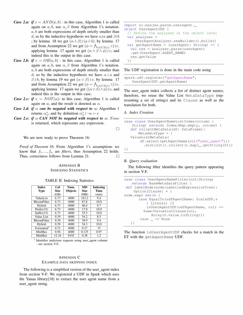
APPENDIX BINDEXING STATISTICS

TABLE II: Indexing Statistics

Index Col Num. MD IndexingType Size Objects Size Time

(GB) (MB) (min)ValueList 6.73 4000 163.2 9.4

BloomFilter 6.73 4000 67.8 10.0Hybrid 6.73 4000 40.4 9.7

Prefix(15) 6.73 4000 17.0 10.0Suffix(15) 6.73 4000 35.5 10.0Value List 0.39 4000 34.2 8.5

BloomFilter 0.39 4000 38.9 9.4Hybrid 0.39 4000 34.3 10.0

Formatted1 0.72 4000 0.27 15MinMax 0.56 4000 0.125 0.97MinMax 12.16 8192 0.38 1.2

1 Identifies malicious requests using user agent column- see section V-F.

APPENDIX CEXAMPLE DATA SKIPPING INDEX

The following is a simplified version of the user agent indexfrom section V-F. We registered a UDF in Spark which usesthe Yauaa library[18] to extract the user agent name from auser agent string.

import nl.basjes.parse.useragent._object UserAgentUDF {// Define the analyzer at the object levelval analyzer =

UserAgentAnalyzer.newBuilder().build()val getAgentName = (userAgent: String) => {val res = analyzer.parse(userAgent).get(UserAgent.AGENT_NAME)res.getValue

}}

The UDF registration is done in the main code using

spark.udf.register("getAgentName",UserAgentUDF.getAgentName)

The user agent index collects a list of distinct agent names,therefore, we reuse the Value List MetaDataType (rep-resenting a set of strings) and its Clause as well as thetranslation for both.

A. Index Creation

case class UserAgentNameListIndex(column :String) extends Index(Map.empty, column) {def collectMetaData(df: DataFrame):

MetadataType = {ValueListMetaData(

df.select(getAgentName(col("user_agent"))).distinct().collect().map(_.getString(0)))

}}

B. Query evaluation

The following filter identifies the query pattern appearingin section V-F.

case class UserAgentNameFilter(col:String)extends BaseMetadataFilter {

def labelNode(node:LabelledExpressionTree):Option[Clause] = {

node.expr match {case EqualTo(udfAgentName: ScalaUDF,v

: Literal) ifisUserAgentUDF(udfAgentName, col) =>

Some(ValueListClause(col,Array(v.value.toString)))

case _ => None}}

The function isUserAgentUDF checks for a match in theET with the getAgentName UDF.