extracting a mobility model from real user traces

Extracting a mobility model from real user tracesMinkyong Kim

Dept. of Computer ScienceDartmouth College

Hanover, [email protected]

David KotzDept. of Computer Science

Dartmouth CollegeHanover, NH

[email protected]

Songkuk KimWilson Center for Research & Technology

Xerox CorporationWebster, NY

[email protected]

Abstract— Understanding user mobility is critical for simula-tions of mobile devices in a wireless network, but current mobilitymodels often do not reflect real user movements. In this paper,we provide a foundation for such work by exploring mobilitycharacteristics in traces of mobile users. We present a method toestimate the physical location of users from a large trace of mobiledevices associating with access points in a wireless network. Usingthis method, we extracted tracks of always-on Wi-Fi devices froma 13-month trace. We discovered that the speed and pause timeeach follow a log-normal distribution and that the direction ofmovements closely reflects the direction of roads and walkways.Based on the extracted mobility characteristics, we developed amobility model, focusing on movements among popular regions.Our validation shows that synthetic tracks match real tracks witha median relative error of 17%.

I. INTRODUCTION

The purpose of mobile computing and communications isto allow people to move about and yet be able to interact withinformation, services, and other people. Anyone designing anapplication, system, or network to serve mobile users musttherefore have some notion about how the users, and theirdevices, move. Indeed, most researchers use simulation todiscover how their application, system or network respondsto variations in user activity, including mobility. It is thuscritical to support such simulations with a realistic model ofuser mobility—and yet, most mobility models used by thisresearch community are ad hoc creations based on the intuitionof their designer. Few models are derived from traces of realuser behavior. The mobile and ad-hoc networks (MANET)community depends on simple but unrealistic variations ofrandom-walk models, for example. An alternative to model-based simulation may be trace-driven simulation. Althoughtrace-driven simulation does not require a mobility model,model-based simulation allows researchers to explore a largerparameter space.

To develop a mobility model, we must understand user mo-bility. We must obtain detailed mobility data about real users,and carefully characterize their mobility. This characterizationprovides useful insights itself, for example, to researchersinterested in predicting mobility in support of location-awareapplications [1] or for network optimization [2]. Recent re-search in opportunistic ad hoc networking also depends on anunderstanding of user mobility and the opportunities for userdevices to interact when users pass close to each other. Somerecent work [3] distributed portable devices to real people to

collect data about such opportunities, but these studies arebased on small populations. One study [4] examines the largetraces collected at Dartmouth College [5], [6] and UCSD [7],but only recognizes opportunities when the users are at thesame Wi-Fi access point (AP), in contrast to when the usersare within communication range of each other.

This paper describes our experiences in extracting user mo-bility characteristics from wireless network traces (syslog) anddeveloping a mobility model based on these characteristics. Wechose to use syslog traces because these traces are relativelyeasy to collect for large user populations; for example, thetraces collected at Dartmouth College contain data from nearly10,000 users over several years. Any wireless ISP provider alsohas access to similar data.

Although syslog traces are readily available, we cannotextract mobility characteristics directly from them. Thesetraces contain sequences of access points with which wirelessdevices associated. From these sequences, we need to extractlocations of users over time. We explored several methods toextract mobility tracks from syslog traces.

We also developed a heuristic to extract mobility charac-teristics from mobility tracks. From these traces we cannotknow whether a user was moving or not, so we need a wayto estimate pause durations. We validate this heuristic usingthe data collected by controlled walks and then apply theheuristic to our wireless network traces to collect mobilitycharacteristics.

We analyzed mobility characteristics including pause time,speed, and direction of movements. We found that pause timeand speed distributions each follow a log-normal distribution.Not surprisingly, the directions of movement do not followa uniform distribution, although many MANET researchersmake that assumption in their simulations. Instead, the di-rections of movement follow the direction of popular roadsand walkways on the campus, and shows a strong symmetryacross 180 degrees. These mobility characteristics provide thefundamental information that underlies any mobility model.

For our mobility model, we first define popular regions,hotspots, and characterize these regions. We concentrate onmovements among hotspots, supposedly more interesting re-gions for many applications. Researchers who want to simulatehow users aggregate (e.g., a friend-finder application [8]) needto have this type of model. Those who want to explore aspectsof context-aware systems (such as scalability of context-aware

This full text paper was peer reviewed at the direction of IEEE Communications Society subject matter experts for publication in the Proceedings IEEE Infocom.

1-4244-0222-0/06/$20.00 (c)2006 IEEE

Authorized licensed use limited to: Dartmouth College. Downloaded on November 27, 2008 at 01:15 from IEEE Xplore. Restrictions apply.

services [9]) can also benefit from such a model.Finally, we use mobility characteristics to develop a soft-

ware model that generates realistic user mobility tracks. Wevalidate our model by comparing synthetic tracks with realtracks. Our validation shows that synthetic tracks match realtracks with a median relative error of 17%.

II. COLLECTING USER TRACES

We use the wireless network data set collected at DartmouthCollege to derive mobility information. The Dartmouth tracedata is the largest publicly-available set of Wi-Fi networktraces, comprising syslog, SNMP and tcpdump data that hasbeen collected since 2001 [5], [6]. In this paper, we concentrateon the syslog data collected from the beginning of June2003 to the end of June 2004. At the time, the DartmouthWLAN consisted of approximately 560 access points (thenumber of APs changes over time as the network evolves).Whenever clients authenticate, associate, roam, disassociateor deauthenticate with an AP, a syslog message is recorded,containing a timestamp in seconds, the client MAC address,the AP name and the event type. Note that syslog traces do notcontain signal-strength information, which would have beenuseful for locating clients.

The Dartmouth trace data includes a map, indicating the(x, y, z) coordinate of most of the APs on campus. We definea location as a pair of (x, y) coordinates on the map. (Weignore the z coordinate, an integer representing the buildingfloor on which the AP is located, in our study; we hopeto extend our approach to three dimensions in future work.)If a map of access points is not available, one can collectlocation of APs through methods such as war-driving (asused by Place Lab [10], [11]), or using AP position-estimationtechniques [12].

For the purposes of characterizing mobility, we are onlyinterested in a subset of wireless network users: the Voice-over-IP (VoIP) device users. Most of the Dartmouth wirelessnetwork clients are laptop users, but most of these clientsare not very mobile, or are nomadic in their mobile networkusage. We chose to concentrate on the always-on VoIP deviceusers, as these have been shown to have higher mobility [5].We obtained a list of 198 MAC addresses belonging to Cisco7920 Wi-Fi VoIP telephones and Vocera VoIP communicators,and only considered syslog data containing one of these MACaddresses.

For each VoIP-client MAC address in the trace data, weextracted the syslog events for each day. To remove diurnaleffects where a client will be less mobile at night (for instance,where the owner of a VoIP device goes home off-campus atnight but leaves the device charging in their office), we onlyconsider the working day by ignoring any events before 8 AMand after 6 PM on each day.

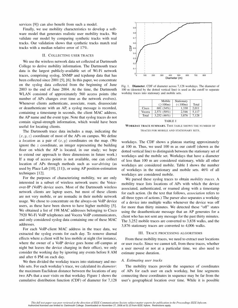
We then divided the workday traces into stationary and mo-bile sets. For each workday’s trace, we calculated its diameter:the maximum Euclidean distance between the locations of anytwo APs that a user visits on that workday. Figure 1 shows thecumulative distribution function (CDF) of diameter for 7,128

0 100 200 300 400 500 600 700 8000

0.1

0.2

0.3

0.4

0.5

0.6

0.7

0.8

0.9

1

Diameter (m)

CD

F

Fig. 1. Diameter. CDF of diameter across 7,128 workdays. The diameter of100 m (denoted by the dotted vertical line) is used as the cutoff to separateworkday traces into stationary and mobile sets.

Mobile Stationary(≥100m) (<100m) Total

Cisco 681 (34%) 1,330 2,011Vocera 2,571 (50%) 2,546 5,117Total 3,252 (46%) 3,876 7,128

TABLE I

WORKDAY TRACE SUMMARY. THIS TABLE SHOWS THE NUMBER OF

TRACES FOR MOBILE AND STATIONARY SETS.

workdays. The CDF shows a plateau starting approximatelyat 100 m. Thus, we used 100 m as our cutoff (shown as thedotted vertical line) to distinguish between the stationary set ofworkdays and the mobile set. Workdays that have a diameterof less than 100 m are considered stationary, while all otherworkdays are considered mobile. Table I shows the numberof workdays in the stationary and mobile sets. 46% of allworkdays are considered mobile.

We parsed these syslog traces to obtain mobility traces. Amobility trace lists locations of APs with which the deviceassociated, authenticated, or roamed along with a timestampfor each action. (In the text that follows, association refers toall three types of actions.) The parser also separates a workdayof a device into multiple walks whenever the device was offfor more than thirty minutes. We detected these “off” statesusing the deauthenticate message that an AP generates for aclient who has not sent any message for the past thirty minutes.The 3,252 mobile traces are converted to 3,838 walks, and the3,876 stationary traces are converted to 4,006 walks.

III. TRACE PROCESSING ALGORITHMS

From these mobility traces, we need to extract user locationsor user tracks. Since we cannot tell, from these traces, whethera user moved or not at a particular time, we also need toestimate pause duration.

A. Estimating user tracks

The mobility traces provide the sequence of coordinatesof APs for each user on each workday, but line segmentsconnecting these coordinates in sequence may be far from theuser’s geographical location over time. While it is possible

This full text paper was peer reviewed at the direction of IEEE Communications Society subject matter experts for publication in the Proceedings IEEE Infocom.Authorized licensed use limited to: Dartmouth College. Downloaded on November 27, 2008 at 01:15 from IEEE Xplore. Restrictions apply.

GPS trackAPs

Fig. 2. AP associations. A pedestrian carried a Vocera communicator on anoutdoor walk around campus. This figure shows line segments between APsthe Vocera associated in sequence.

to estimate the location of a Wi-Fi user by having its clientsense multiple nearby APs (as with Place Lab [10] and manyothers), it is experimentally difficult to obtain such locationtraces from thousands of users. In contrast, syslog data, whichis recorded by the AP, is readily available. Thus, we exploremethods to estimate user locations from syslog data.

There are several reasons that locations in syslog datamay be different from a user’s location. First, most usersdo not stand next to an AP, and then walk to a point nextto another AP. Second, mobile devices do not necessarilyassociate with the geographically-closest AP. This behaviorresults from many reasons, such as different APs being con-figured with different power levels, or the signal from closeAPs being blocked by buildings or trees. Third, differentdevices have different aggressiveness in changing associations.Less-aggressive devices do not change the associated AP asfrequently. Thus, they may be associated with an AP far fromthe user’s current location.

To get a sense of how VoIP devices change associations,we asked a volunteer to walk around on the Dartmouthcampus with a GPS device and a Vocera communicator. Afterregistering the GPS data to the AP map coordinates, we plottedthe actual path (according to GPS) and the associations in thesame figure. Figure 2 shows both the GPS track and the crudetrack of a user’s location by drawing line segments betweenthe map coordinates of APs in sequence; the arrow shows thedirection of the walk. Clearly, a mobile user roams widelyfrom AP to AP. This crude method estimates a mobility trackthat is far from the GPS track.

Based on the above observations, we need a method toestimate a smooth path representing the user’s location overtime. We explore three approaches to address this problem.

1) Triangle centroid: The centroid algorithm uses locationof past three AP associations as the vertices of a triangle. Weestimate the user’s location as the centroid of a triangle, whichis the intersection of the triangle’s three triangle medians. Thelocation estimate is updated whenever there is an associationmessage.

2) Time-based centroid: Because devices do not changeassociations periodically, using the past three associations maybe ineffective, especially for less aggressive devices. Thus, weexplore the centroid algorithm with a window of a fixed-timeperiod, q. Every p seconds, we update the user’s location withassociations that happened during the past q seconds. Thus, auser’s location at time t is defined as:

x(t) = 1n

∑ni=1 xi, y(t) = 1

n

∑ni=1 yi (1)

where n is the number of associations within the past qseconds. If there has been no association within the past qseconds (n = 0), we keep the previous location estimate:

x(t) = x(t − p), y(t) = y(t − p). (2)

The default values for p and q are 10 and 60 seconds,respectively. Note that n changes dynamically for each updatefor this method, while n is fixed at three for the trianglecentroid algorithm.

3) Kalman filter: A Kalman filter is a recursive data pro-cessing algorithm that produces optimal estimates. While thisfilter requires significant knowledge of the system, one canmake reasonable guesses to get a good result.

The system to be estimated can be modeled as:

xk+1 = Φkxk + wk (3)

where xk represents the state of the system, Φ is a matrixrelating one state xk to the next state xk+1, and w is avector representing system noise. Our state variables includethe user’s location (x and y) and velocity (x′ and y′). Then,Equation 3 is written as:

xx′

yy′

k+1

=

1 t 0 00 1 0 00 0 1 t0 0 0 1

k

xx′

yy′

k

+

w1

w2

w3

w4

k

(4)

where t is the time difference between two consecutive asso-ciations.

The measurement of the system is defined as:

zk = Hkxk + vk (5)

where H is a matrix relating the state variables xk to themeasurements zk, and v is a vector representing measurementerror. For each association k, we have the location of the APwith which a user is associated. Given this measurement, weupdate our estimate of the user’s location. Since the measuredlocation can be considered as the user’s true location disturbedby some noise, Equation 5 can be written as:

[z1

z2

]k

=[

1 0 0 00 0 1 0

]k

xx′

yy′

k

+[

v1

v2

]k

. (6)

We now need to define the covariance matrices for wk

and vk, Qk and Rk, respectively. Q represents the degreeof variability in the state variables; R represents the measure-ment uncertainty. Since the relationship between variances is


Fig. 3. GPS tracks. This figure shows the GPS tracks of four walks depictedon the Dartmouth campus map.

unknown, we assume that the variances are independent ofeach other, making their products zero. The resulting Q andR are:

Qk =

w12 0 0 0

0 w22 0 0

0 0 w32 0

0 0 0 w42

Rk =[

v12 0

0 v22

]

Since it is the relative magnitude of values in covariancematrices that affects the filter’s performance, we set values inQ to one and empirically chose values for R in the followingsection.

4) Validation: To validate path extractors, we walkedaround on the Dartmouth campus with a GPS device, aVocera VoIP communicator, and a Cisco VoIP phone. GPSdata serves as the ground truth and VoIP data is used toestimate a user’s path. We have data for four such walks,each made by a different person along a different path. Eachwalk lasted around 30 minutes, roughly 20 minutes walkingand 10 minutes pausing at an indoor location. With these fourwalks, we were able to visit much of the area covered by thecampus-wireless network. Figure 3 shows the GPS tracks ofthese walks on our campus map.

To get the difference between the tracks and GPS data, wecomputed the distance between the two every 30 seconds.Since there is no GPS data when a user was indoors, weexcluded these time periods from the calculation. (Thesepause-time periods are later used to test our characterizationtechnique.) Figure 4 illustrates the distance between a GPStrack and an estimated track of a Vocera communicator forone of our walks.

Choosing Kalman parameters: We used all four walks tochoose the Kalman parameters. Since movements in x and ydirections are likely to be symmetric, we assume that errorsin the x and y directions are same. Then, we have only oneunknown variable, v2.

Fig. 4. Differences. This figure shows the difference between the GPS trackand the path estimated using a Kalman filter.

Figure 5 shows the median difference between the GPStrack and the path estimated by Kalman filters with differentv2 values: 15, 25, 35, 50, 100, 150, 200, and 250. All users,except User 4, do not show a trend over different values ofv2. For User 4, as v2 increases, the difference decreases forthe Vocera while it increases for the Cisco phone; there is notone good value for both. Thus, we chose 25 for v2 based onthe local minimum observed for some of the Vocera users.

Evaluating path extractors: From our walks, we found thatdifferent types of devices have different association patterns.Vocera communicators aggressively associated with manyAPs, while the Cisco phones tended to stay associated witha single AP for a long time. Path extractors should be ableto cope with these differences. We also observed that thedistance from a device to the associated AP varies by a largeamount; while a device tends to associate with nearby APs, itsometimes associated with APs as far as 200 meters away. Pathextractors should be able to produce estimates with a boundederror range by coping with associations with far-away APs.

Figure 6 shows the difference result for Vocera commu-nicators and Cisco phones; each line shows the median andmaximum of differences (measured every 30 seconds) foreach user. The triangle centroid, time-based centroid, andKalman filter are labeled as ‘triangle’, ‘time’, and ‘kalman’,respectively. In addition to these three algorithms, we includeda crude track by connecting the locations of APs (like thatshown in Figure 2); this track is labeled as ‘ap’.

The triangle-centroid algorithm produces relatively well-bounded estimates for Vocera communicators, but its mediansfor Cisco phones are much worse than the crude tracks. Thisresult happens because Cisco phones tend to stay associatedwith an AP for a while, so using the past three associationsis too slow to reflect a user’s current location. The time-basedcentroid algorithm works better than the triangle-centroidalgorithm for Cisco phones, but it sometimes updates the user’slocation with far-away APs as happened for Vocera User 2and User 4. The Kalman filter produces estimates that arewell bounded for Vocera communicators and it also worksreasonably well for Cisco phones.


18

20

22

24

26

28

30

32

0 50 100 150 200 250

Diff

eren

ce (

met

er)

v2

user 1user 2user 3user 4

(a) Vocera

32

34

36

38

40

42

44

46

48

50

0 50 100 150 200 250

Diff

eren

ce (

met

er)

v2

user 1user 2user 3user 4

(b) Cisco phone

Fig. 5. Kalman parameter. This figure shows the median difference betweenthe GPS track and the estimated path with different v2 values.

B. Extracting pause time

We then used the Kalman filter to extract user tracks, whichare sequences of a user’s locations with timestamps indicatingwhen the user arrived at each location. To characterize usermobility, we need to separate the time between two consec-utive associations into travel time and pause time. Since wecannot tell whether a user was moving by looking at the traces,we need to estimate pause duration.

1) Algorithm: We estimate pause duration using the user’sspeed. If the speed between two locations is within a “normal”range, we assume that the user did not pause at the sourcelocation. If the speed is too slow, we assume that the userdid not move at that slow speed, but instead, paused at thesource before moving to the destination. When considering a“normal” range, we assume that users are pedestrians. Thisassumption is reasonable for the Dartmouth campus; mostpeople walk rather than drive a car or take a bus on the campusbecause the campus is small. For an environment where userschange their mode of transportation, we can adapt methodsthat detect mode of transit [13], [14].

Our track traces consists of an arrival time ti and locationli, defined as (xi, yi). When a user arrives at li+1 at ti+1, the

1 2 3 40

20

40

60

80

100

120

140

160

180

200

User

Diff

eren

ce (

met

er)

aptriangletimekalman

(a) Vocera

1 2 3 40

20

40

60

80

100

120

140

160

180

200

User

Diff

eren

ce (

met

er)

aptriangletimekalman

(b) Cisco phone

Fig. 6. Path extractors This figure shows median(‘x’) and maximum(‘o’)of differences for Vocera communicators and Cisco phones.

speed from li to the new location li+1 is computed as

si =di

ei(7)

where di is the Euclidean distance between li and li+1, and ei

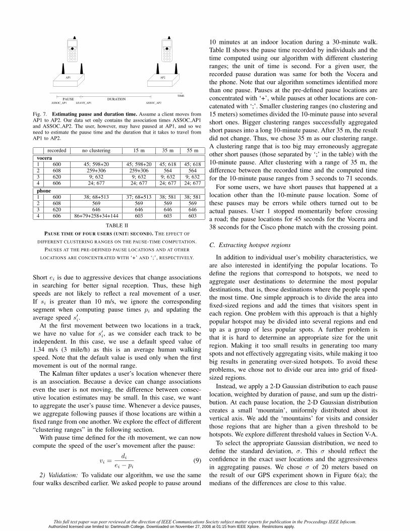
is the elapsed time, ti+1− ti. If si is within the normal range,we assume that the user did not pause at li. We defined thenormal range to be min ≤ si ≤ 10 m/s; we explored differentvalues of min: 0.1 m/s and 0.5 m/s. If si is smaller than min,the user is likely to have paused at li before moving to li+1.Thus, bigger min values are likely to produce more pauses.The elapsed time, ei, is the sum of the pause time, pi, andthe duration of travel, qi, as illustrated in Figure 7. The pausetime, pi is computed as

pi = ei − qi = ei − di

s′i(8)

where s′i is the average speed of the user, computed as expo-nentially weighted moving average: s′i = 0.25si + 0.75s′i−1.

In the traces we sometimes observe slow speeds due topauses, but we also observe some high speeds. These highspeeds are observed only with short ei (a few seconds).Obviously, short ei produces high speed (see Equation 7).


PAUSE DURATIONASSOC_AP2

TIME

ASSOC_AP1 LEAVE_AP1

AP1 AP2

Fig. 7. Estimating pause and duration time. Assume a client moves fromAP1 to AP2. Our data set only contains the association times ASSOC AP1and ASSOC AP2. The user, however, may have paused at AP1, and so weneed to estimate the pause time and the duration that it takes to travel fromAP1 to AP2.

recorded no clustering 15 m 35 m 55 m

vocera1 600 45; 598+20 45; 598+20 45; 618 45; 6182 608 259+306 259+306 564 5643 620 9; 632 9; 632 9; 632 9; 6324 606 24; 677 24; 677 24; 677 24; 677

phone1 600 38; 68+513 37; 68+513 38; 581 38; 5812 608 569 569 569 5693 620 646 646 646 6464 606 86+79+258+34+144 603 603 603

TABLE II

PAUSE TIME OF FOUR USERS (UNIT: SECOND). THE EFFECT OF

DIFFERENT CLUSTERING RANGES ON THE PAUSE-TIME COMPUTATION.

PAUSES AT THE PRE-DEFINED PAUSE LOCATIONS AND AT OTHER

LOCATIONS ARE CONCENTRATED WITH ‘+’ AND ‘;’, RESPECTIVELY.

Short ei is due to aggressive devices that change associationsin searching for better signal reception. Thus, these highspeeds are not likely to reflect a real movement of a user.If si is greater than 10 m/s, we ignore the correspondingsegment when computing pause times pi and updating theaverage speed s′i.

At the first movement between two locations in a track,we have no value for s′i, as we consider each track to beindependent. In this case, we use a default speed value of1.34 m/s (3 mile/h) as this is an average human walkingspeed. Note that the default value is used only when the firstmovement is out of the normal range.

The Kalman filter updates a user’s location whenever thereis an association. Because a device can change associationseven the user is not moving, the difference between consec-utive location estimates may be small. In this case, we wantto aggregate the user’s pause time. Whenever a device pauses,we aggregate following pauses if those locations are within afixed range from one another. We explore the effect of different“clustering ranges” in the following section.

With pause time defined for the ith movement, we can nowcompute the speed of the user’s movement after the pause:

vi =di

ei − pi(9)

2) Validation: To validate our algorithm, we use the samefour walks described earlier. We asked people to pause around

10 minutes at an indoor location during a 30-minute walk.Table II shows the pause time recorded by individuals and thetime computed using our algorithm with different clusteringranges; the unit of time is second. For a given user, therecorded pause duration was same for both the Vocera andthe phone. Note that our algorithm sometimes identified morethan one pause. Pauses at the pre-defined pause locations areconcentrated with ‘+’, while pauses at other locations are con-catenated with ‘;’. Smaller clustering ranges (no clustering and15 meters) sometimes divided the 10-minute pause into severalshort ones. Bigger clustering ranges successfully aggregatedshort pauses into a long 10-minute pause. After 35 m, the resultdid not change. Thus, we chose 35 m as our clustering range.A clustering range that is too big may erroneously aggregateother short pauses (those separated by ‘;’ in the table) with the10-minute pause. After clustering with a range of 35 m, thedifference between the recorded time and the computed timefor the 10-minute pause ranges from 3 seconds to 71 seconds.

For some users, we have short pauses that happened at alocation other than the 10-minute pause location. Some ofthese pauses may be errors while others turned out to beactual pauses. User 1 stopped momentarily before crossinga road; the pause locations for 45 seconds for the Vocera and38 seconds for the Cisco phone match with the crossing point.

C. Extracting hotspot regions

In addition to individual user’s mobility characteristics, weare also interested in identifying the popular locations. Todefine the regions that correspond to hotspots, we need toaggregate user destinations to determine the most populardestinations, that is, those destinations where the people spendthe most time. One simple approach is to divide the area intofixed-sized regions and add the times that visitors spent ineach region. One problem with this approach is that a highlypopular hotspot may be divided into several regions and endup as a group of less popular spots. A further problem isthat it is hard to determine an appropriate size for the unitregion. Making it too small results in generating too manyspots and not effectively aggregating visits, while making it toobig results in generating over-sized hotspots. To avoid theseproblems, we chose not to divide our area into grid of fixed-sized regions.

Instead, we apply a 2-D Gaussian distribution to each pauselocation, weighted by duration of pause, and sum up the distri-bution. At each pause location, the 2-D Gaussian distributioncreates a small ‘mountain’, uniformly distributed about itsvertical axis. We add the ‘mountains’ for visits and considerthose regions that are higher than a given threshold to behotspots. We explore different threshold values in Section V-A.

To select the appropriate Gaussian distribution, we need todefine the standard deviation, σ. This σ should reflect theconfidence in the exact user locations and the aggressivenessin aggregating pauses. We chose σ of 20 meters based onthe result of our GPS experiment shown in Figure 6(a); themedians of the differences are close to this value.


102

103

104

10−4

10−3

10−2

10−1

100

Pause (s)

CC

DF

min=0.1m/s, not clusteredmin=0.1m/s, clusteredmin=0.5m/s, not clusteredmin=0.5m/s, clustered

Fig. 8. Pause. This figure shows the overall pause-time distribution.

IV. MOBILITY CHARACTERISTICS

Having verified that the Kalman filter provides a reasonableapproximation of the GPS data, we apply this filter to the 3,838mobile walks to produce the same number of mobility tracks.We then apply our pause-time estimator and extract mobilitycharacteristics: pause time, speed, direction, start time, andend time.

For the 4,006 stationary walks, we do not extract user tracks.We estimate each user’s stationary location using the simpletriangle centroid (Section III-A.1). We extract characteristicssuch as duration of stay, start time, and end time.

A. Mobile set

For both pause time and speed characterization, we usethe complementary cumulative distribution function (CCDF):F (x) = P (X ≥ x). CCDF is commonly drawn on alogarithmic scale for both axes. The log-log CCDF helpsdetermine whether a set of data fits a power law or heavy-tailed distribution; if the data is linear on a log-log scale, thenthis means that the data fits a power-law distribution.

Figure 8 shows the log-log CCDF of the number of pausesobserved across all 3,838 walks as a function of pause durationin seconds. We explored two different values of min, usedfor our pause-time estimator (see Section III-B.1). Note thatwe only counted non-zero pauses. This figure shows thedistributions of pauses both before and after clustering, usingthe clustering range of 35 meters (based on the validationpresented in Section III-B.2). As expected, there were morelonger pauses when clustered. min of 0.5 m/s producedrelatively more shorter pauses than min of 0.1 m/s; this isbecause bigger min identifies more pauses. It is clear thatnone of distributions are linear. Using maximum likelihoodestimation (MLE), we find that the clustered pauses fit a log-normal distribution, with a small number of users pausing forlong periods of time.

Figure 9 shows the weighted log-log CCDF of the totalduration of travel as a function of speed in meters per second.It includes distributions with min of 0.1 m/s and 0.5 m/s. The

10−1

100

101

10−4

10−3

10−2

10−1

100

Speed (m/s)

CC

DF

min=0.1m/smin=0.5m/s

Fig. 9. Speed. This figure shows the overall speed distribution. The speedof each movement segment is weighted by duration of that movement.

0.01

0.02

0.03

0.04

30

210

60

240

90

270

120

300

150

330

180 0

Fig. 10. Direction. This figure shows a weighted PDF of movement directionwith a bin size of 5°. The direction of each movement segment is weightedby duration of that movement.

speed of each movement segment is weighted by the durationof that movement. min of 0.5 m/s produced more faster speedsthan min of 0.1 m/s. The median for min of 0.5 m/s and0.1 m/s are 0.43 m/s and 1.26 m/s, respectively; 1.26 m/s(2.8 mile/h) is close to the average human walking speed(3 mile/h). MLE finds that speed fits a log-normal distribution.

Figure 10 shows the probability density function (PDF)of movement directions. The direction of each movement isweighted by the duration of that movement. The bin size is 5°.By manual comparison to a map of the Dartmouth campus,we found that the directions with larger peaks correspond tothe directions of popular roads. Interestingly, the trends arerepeated every 180°. We expect that this symmetry is becauseon a given road, people move in both directions. For instance,on a road that goes south and north, people move eithernorthward or southward, generating peaks at two directionsthat are exactly 180° apart. Because of this symmetry, boththe mean and median of the distribution are close to 0°.

Figure 11 shows a CDF of the start time and end time ofeach of 3,252 mobile workday traces. The line ‘start’ shows


8 9 10 11 12 13 14 15 16 17 180

0.1

0.2

0.3

0.4

0.5

0.6

0.7

0.8

0.9

1

Hour

CD

F

startend

Fig. 11. Start and end times of mobile workdays. This figure showsthe CDF across 3,219 workdays. ‘start’ denotes the time that devices firstappeared within a workday; ‘end’ shows the time that devices disappeared.

Fig. 12. Mobile users on map.

the time that devices first appeared within a workday. The line‘end’ shows the time that devices disappeared. Note that ourchosen workday runs from 08:00 to 18:00; earlier start timeswere recorded as 08:00 and later end times as 18:00. 47% ofworkdays started by 09:00, and 53% ended after 17:00.

Figure 12 shows the distribution of pauses over our campusafter applying a Gaussian distribution for each visit andadding them up. The darker spots represent higher mountains.The popular regions include the main Dartmouth library, theDepartment of Computer Science, the School of Engineering,the building with offices of network administrators, a hotelrestaurant, and a gym.

B. Stationary set

We computed the duration of the stay for each of 4,006walks. The duration of a walk is the difference between thetime when the first and last messages of that walk wererecorded. When there is only one message, the duration iszero. Note that this duration is an approximation of the timethat a device was connected to the network. Since APs donot always generate deauthentication messages, which showthe time that clients deauthenticate, we cannot rely on thesemessages to determine when clients went off. For example,

0 1 2 3 4 5 6 7 8 9 100

0.1

0.2

0.3

0.4

0.5

0.6

0.7

0.8

0.9

1

Duration (hour)

CD

F

Fig. 13. Duration of stay. The CDF of overall duration of stay across 4,006stationary walks. The vertical dotted line shows the thirty-minute timeout usedby APs to deauthenticate clients with no activities.

8 9 10 11 12 13 14 15 16 17 180

0.1

0.2

0.3

0.4

0.5

0.6

0.7

0.8

0.9

1

Hour

CD

F

startend

Fig. 14. Start and end times of stationary workdays. This figure showsthe CDF across 3,876 workdays. ‘start’ and ’end’ denote the time that devicesfirst appeared and the time that devices disappeared within a workday.

if a device associates with an AP and no deauthenticationmessage was generated, the computed duration for that devicemay be much shorter than the actual duration that the devicewas connected to the network.

Figure 13 shows the CDF of duration for 4,006 walks.About 29% had a duration of less than two minutes. Thejump at thirty minutes is due to the fact that a client isdeauthenticated if it has not sent any message for thirtyminutes. After the thirty minute jump, the number of walksfor different durations does not change much.

Figure 14 shows the CDF of start and end time for 3,876stationary workdays. 28% of workdays started by 09:00 and34% ended after 17:00. Compared to mobile workdays, sta-tionary workdays started later and ended earlier. This resultmay be because workdays that start later and end earlier aremore likely to have small diameters, and thus are classified asstationary.

Figure 15 shows the users’ locations on the campus mapafter applying a Gaussian distribution for each stationarylocation. For this set of walks, we used the triangle centroid to


Fig. 15. Stationary users on map. The arrow denotes a popular region thatis unique to stationary users.

compute the stationary location for each walk and calculatedthe number of walks at each location. Note that we did notconsider the duration of stay for this set; each stationary lo-cation is weighted equally. Compared to the popular locationsfor mobile users (shown in Figure 12), the popular stationarylocations are restricted to smaller regions. Nonetheless, thesepopular locations for stationary users coincide with those formobile users. The only location that is unique for the stationaryusers is one of the clusters of undergraduate dorms, denotedby an arrow in Figure 15. The locations that were popularamong mobile users, but not among stationary users, includea gym and a hotel containing a restaurant.

C. Summary of characteristics

Table III shows the summary of mobility characteristics. Foreach characteristic, we list the mean and median. The last twocolumns show the parameters for fitted distributions and theroot mean square (RMS) error. Most characteristics are fittedas either log-normal distribution or exponential distribution.The equation for the PDF of the log-normal distribution is

f(x) = e−(ln(x−µ)2)/2σ2

xσ√

2π, and that of the exponential distri-

bution is f(x) = eax+b. To fit data to a distribution, wefirst separated them into 100 bins. To remove the effect oftruncating traces to working hours, we ignored the first bin forthe start time, and ignored the last bin for the end time. Thestart and end time of both mobile and stationary sets followexponential distributions. The pause times and speed of themobile set follow log-normal distributions. The durations ofthe stationary set follow a uniform distribution.

V. CHARACTERIZING HOTSPOTS

The research community is often more interested in pop-ular regions, hotspots, where wireless users spend most oftheir time. For example, researchers working in opportunisticnetworking or developing context-aware services need to havean accurate model of these regions. Thus, we focus on thesehotspots in developing a mobility model. We first definehotspot regions using a Gaussian distribution; the area outsideof hotspots becomes the cold region. We then characterizeeach region separately.

4

5

6

7

8

9

10

11

1600 1800 2000 2200 2400

Num

ber

of h

otsp

ots

Threshold

Fig. 16. Threshold for hotspots

A. Defining hotspot regions

Given the map of user destinations (Figures 12 and 15),we need to define hotspot regions by applying a threshold.Threshold values that are too low may generate too many orbig regions as hotspots. Some of these hotspots may be infact not popular locations. On the other hand, if the thresholdvalue is too high, we may also select too many hotspots, asthe threshold may divide a large region into several smallerhotspots.

To observe the effect of selecting different threshold values,we calculated the number of hotspots generated by varying thethreshold from 1500 to 2500 in increments of 100. Figure 16shows the result. Among the values that generated the mini-mum number of hotspots we chose the smallest, 1900; smallervalues produce larger hotspots.

Figure 17 shows the regions represented by these fivehotspots on a map of the Dartmouth campus. These hotspotscoincide with the locations of several buildings popular amongVocera and Cisco phone users: the School of Engineering, themain Dartmouth library, the Computer Science department, thebuilding with offices of campus network administrators, and ahotel containing a restaurant. Note that these hotspots representpopular spots among VoIP device users and may be differentfrom popular spots of the whole Dartmouth population.

B. Hotspot characteristics

Figure 18 shows a PDF of the number of users (walks)starting their day at each region (shown as black bars). Theregion labeled as ‘0’ represents tracks that started outside anyhotspot (the cold region); the rest represents values for eachhotspot. This figure also shows the area of each hotspot regionnormalized by the total area of all hotspots (shown as whitebars). The size of the cold region is not included because wedo not have a clear boundary of the campus and thus do notknow the exact size of the cold region. Clearly, we see that thenumber of users and the hotspot size follow a similar trend,perhaps because a popular hotspot builds a larger ‘mountain’with a larger base.

We also computed the pause-time distribution for each


set characteristic unit mean median distribution RMS

mobile start hour 1.9 (09:54) 1.1 (09:06) exponential a = −0.438 b = −0.872 0.5399end hour 8.5 (16:30) 9.1 (17:06) exponential a = 0.523 b = −6.637 0.1844

pause (min=0.1m/s) hour 0.718 0.223 log-normal µ = −1.880 σ2 = 5.085 1.1654pause (min=0.5m/s) hour 0.466 0.045 log-normal µ = −2.700 σ2 = 4.738 3.0781speed (min=0.1m/s) m/s 0.76 0.43 log-normal µ = −0.741 σ2 = 0.788 0.5252speed (min=0.5m/s) m/s 1.64 1.26 log-normal µ = 0.290 σ2 = 0.604 0.5253

direction degree -6.2° 2.5° - -

stationary start hour 3.3 (11:18) 2.4 (10:24) exponential a = −0.175 b = −1.599 0.3754end hour 7.3 (15:18) 8.4 (16:24) exponential a = 0.249 b = −3.858 0.5246

duration (after 30 minutes) hour 5.1 5.0 uniform f(x) = 0.1055 0.3802

TABLE III

SUMMARY OF MOBILITY CHARACTERISTICS.

Fig. 17. Hotspots on campus map. This shows the hotspots identified withthe threshold of 1900. Hotspots 1 to 5, in order, correspond to a hotel, theSchool of Engineering, the main Dartmouth library, the Computer Sciencedepartment, and the building with offices of campus network administrators.

0 1 2 3 4 50

0.05

0.1

0.15

0.2

0.25

0.3

0.35

0.4

Region

Pro

babi

lity

Initial usersHotspot size

Fig. 18. Initial regions. This figure shows the initial region distribution ofthe number of users for each region. ‘0’ represents regions outside of fivehotspots.

region. Figure 19 shows CDFs of pause time for five hotspotsand the cold region. We first aggregated pause time as longas a user remains within the same region. The aggregatedpause time depicts the duration of a user’s stay after enteringa region. For each region, we have a CDF of the number ofaggregated pauses for all walks as a function of aggregatedpause duration. We include pause times of zero seconds; weneed this information for simulation to decide whether to pauseor not before moving to the next location. Figure 19 showsthat the cold region has relatively more short pauses than anyof the hotspots. This result is expected since we chose hotspots

0 0.5 1 1.5 2 2.5 3 3.5

x 104

0

0.1

0.2

0.3

0.4

0.5

0.6

0.7

0.8

0.9

1

Pause (s)C

DF

coldhot 1hot 2hot 3hot 4hot 5

Fig. 19. Pause distribution per region. This figure shows the CDF of pausetime for five hotspots and the cold region.

as regions that have longer total pause times. Among the fivehotspots, hotspot 2 and 3 have more long pauses. This impliesthat people tend to stay for a long time in these two regions:the School of Engineering and the main Dartmouth library.

To capture movements between different regions, we com-puted the probability of moving from one region to another. Inaddition to five hotspots and the cold region, we also definedthe OFF state. Thus, we have an n×n transition matrix wheren − 2 is the number of hotspots.

Among these seven states, the cold region is treated differ-ently. It is considered not as a destination, but as a waypointthat a user goes through or stops on the way from onehotspot to another. A waypoint is location li in our tracktraces described in Section III-B.1. For each transition fromone hotspot to another hotspot or OFF state, we count thenumber of waypoints from traces, and generate a (n − 1) ×(n − 1) waypoint matrix that consists of the average numberof waypoints when users moved between two regions.

VI. MODELING MOBILITY

We generate synthetic mobility tracks using our model andthen compare these tracks to the real tracks, using character-istics that were not considered by the model.

A. Generating tracks

To simulate users’ movements, we use the following mo-bility characteristics that we described earlier:


��

��

��

source

waypoints

destination

Fig. 20. Example of a path with three waypoints.

1) Ratio of mobile set size to stationary set size2) Mobile set

• n × n Region transition matrix(where n − 2 is the number of hotspots)

• (n − 1) × (n − 1) Waypoint matrix• Overall speed distribution• Overall start time distribution for mobile workdays• Initial region distribution• Pause time distribution per region

3) Stationary set

• Initial location map• Start time distribution for stationary workdays• Duration of stay

Using these characteristics, we generate synthetic movementtraces. A user is assigned as either mobile or stationary usingthe mobile to stationary ratio. A stationary user enters thenetwork at a time from the start time distribution at the locationfrom the initial location map. She then stays at the locationfor the duration chosen from the duration-of-stay distribution.

A mobile user enters the network at a time selected fromthe start time distribution at a region selected from the initialregion distribution. The user’s next destination is then chosenbased on the probabilities in the region transition matrix.

The number of waypoints visited on the way to the desti-nation is based on the waypoint matrix. We use a Gaussiandistribution with the mean based on this matrix to choosethe number of waypoints, k, for each move. We choose thelocations of k points, uniformly distributed, within the areabounded by a box whose two diagonal end points are definedby the source and the destination of the move. We then sort thek points in ascending order by their distance from the source.Figure 20 shows an example path constructed in such way.We expect that this approach generates paths that are closerto real movements than using straight lines between regions.

The speed of movement is chosen from the overall speeddistribution. Once a user has reached the destination, he pausesfor a period chosen from the pause time distribution forthat particular region. When the pause time elapses, the nextdestination is chosen using the region transition matrix.

B. Validation

One of the most difficult problems in modeling is todetermine whether a model captures reality. For instance, onecould compare the pause-time distributions of both sets oftracks and determine whether they are similar. The pause-timedistribution, however, is a component of the model that created

the generated tracks. We would therefore expect the twodistributions to be similar. Verification [15] is concerned withdetermining whether the conceptual model has been correctlytranslated into a computer program. Although verification isan important step, its purpose is debugging. Instead, one needsto validate a model. Validation is the process of determiningwhether a model is an accurate representation of the system.To validate a model, we need to compare an aspect of thetracks that is not a component of the model.

We validate the tracks by looking at the number of visitorswithin a given region in each hour of a workday. We define thenumber of visitors to be the number of users who either werealready in the region at the start of the hour or entered duringthe hour. Note that a user can be counted at most once for aregion in a given hour. We count the visitors per region perhour for both the generated tracks and the real ones. Note thatthis method does not validate the path (location of waypoints)that a user took to move between hotspots. It also does notvalidate behaviors of stationary users.

Figures 21 shows the number of visitors per region per hour.The x-axis shows one-hour buckets starting at 08:00 and end-ing at 18:00. The number of visitors using the synthetic tracksare similar to the real tracks for all regions except hotspot 1.The number of visitors in the real tracks for these four hotspotsis relatively stable during the day. Visitors increase at thebeginning of the day, are relatively constant during the day,and decrease at the end of the workday. Hotspot 1, however,has a large peak between 1200 and 1300, which may be dueto users visiting a restaurant during their lunch hour. Thesynthetic tracks of hotspot 1 fail to match the real behaviordue to these temporal variations. While our model considersthe variations for the beginning and ending of each workingday, it currently does not consider the variation for certainhours during the day, such as lunch time. Incorporating suchtemporal variations may be useful, although it may requireprior knowledge about a hotspot, such as whether it containsa restaurant, if lunch-time movements are to be considered.

We compute the relative error for each hotspot. Let the valueof a real track be r and that of synthetic track be s. Then, therelative error is defined as

∑ni=1 |ri − si|/

∑ni=1 ri where n

is the number of hour-long bins.Figure 22 shows the relative error between the synthetic

tracks and real tracks. Hotspot 1 with a large peak duringlunch time has the largest error of 46%. The error for therest of the hotspots ranges from 16% to 30%. The median ofrelative error for the five regions is 17%.

VII. RELATED WORK

Most MANET researchers use relatively simple mobilitymodels, based on some form of random walk on a flat plane.With increasing awareness of the limitations of some ofthese models [16] and the importance of a realistic mobilitymodel in the evaluation of MANET protocols [17], othershave begun to propose more complex models. For example,Jardosh et al. propose a random-walk model that incorporatesobstacles [18]. This paper describes a technique for modeling


0

100

200

300

400

500

600

8 9 10 11 12 13 14 15 16 17

visi

tor

hour

Hotspot 1 realsynthetic

0

100

200

300

400

500

600

8 9 10 11 12 13 14 15 16 17

visi

tor

hour

Hotspot 2

0

200

400

600

800

1000

1200

1400

8 9 10 11 12 13 14 15 16 17

visi

tor

hour

Hotspot 3

0

50

100

150

200

250

8 9 10 11 12 13 14 15 16 17

visi

tor

hour

Hotspot 4

0

50

100

150

200

250

8 9 10 11 12 13 14 15 16 17

visi

tor

hour

Hotspot 5

Fig. 21. Hourly visitors. This figure shows the number of visitors duringeach hour of a workday for the five hotspots.

paths between points based on Voronoi diagrams, which couldbe adapted for use in our model. Another mobility modelis proposed by Musolesi et al. [19], who use observationsfrom social networking theory to create a model that reflectshow users congregate according to their social relationships

1 2 3 4 50

0.1

0.2

0.3

0.4

0.5

Hotspot

Rel

ativ

e er

ror

Fig. 22. Relative error. This figure shows the relative error between thesynthetic tracks and the real tracks.

with each other. These complex models, however, are typicallysynthetically generated, rather than based on real traces.

Recently, there have been a few papers describing waysto extract places from traces of user mobility. For exam-ple, Patterson et al. used GPS data in an effort to identifycommon destinations in a user’s daily life [20]; their resultsare interesting, but it is not clear how to use this techniqueto derive a general model for a user population. Similarly,Kang et al. demonstrate a method for clustering a sequenceof location observations to identify “places” within a movinguser’s path [21]. Again, although they validate the techniqueon a trace of two users, their aim is not to build a generalmodel for a larger population.

There have been few significant efforts to create mobilitymodels from real traces. In one short paper, Hsu et al. developa Weighted Way Point model from a set of survey data,in which they asked 268 students to keep a diary of theirmovements on campus for a month, at the granularity of abuilding [22]. Using a predefined set of five location types(classrooms, libraries, cafeterias, off-campus, and other), theynoted a non-uniform distribution of visits to these locationtypes. Their Markov-based model conditions the choice of anext location type upon the time of day (morning or afternoon)and on the current location type. They also used the surveydata to extract a distribution of pause times for each locationtype. They confirm that their model, when used in a simulatorfor ad hoc routing, does demonstrate non-uniform locationdistribution and (due to clustering) leads to lower connectivitythan does the random way-point model. Although our studymust estimate user locations from network-association records,it goes far beyond their study, by extracting mobility fora larger area, with finer location granularity, over a longerperiod of time, and for far more users. Another study based onobservations of pedestrian traffic on a campus [23] developeda hybrid mobility model which favors certain directions basedon probabilities computed from the observations. In this shortpaper, they only observe people at six locations on a largecampus. Using the same trace as our study, Jain et al. [24]developed a model of wireless users’ AP registration patterns,which may be significantly different from users’ physicalmobility patterns. Their model ignores temporal patterns andfocuses only on spatial patterns.


VIII. CONCLUSION

This paper has presented one of the first attempts toconstruct a WLAN mobility model from real-world wirelessuser traces. We present a method for extracting users’ mo-bility tracks from these traces, and validated this method bycomparing them to the location determined by users carryingboth GPS and 802.11 devices. We applied our method toone of the largest available traces of wireless users, fromDartmouth College. By examining the mobility in these trackswe were able to extract information about the movementspeed, pause times, destination transition probabilities, andwaypoints between destinations. This information forms anempirical model that we used to generate synthetic tracks,which we validated by comparison to the real tracks. Wefound that our generated tracks produced similar results to thereal tracks, save in the cases where temporal variations werepresent in the real tracks, as our model does not consider thesetemporal effects.

We believe that this model, and the methods used toconstruct it, will be useful for research in many areas of mobilecomputing and communications. As examples, we cite relatedwork in mobile ad hoc networking, opportunistic networking,content-distribution networks, and location prediction, all ofwhich need good mobility models or an understanding ofmobility characteristics.

In future work, we intend to further improve our metricsfor validating our synthetic tracks. We also intend to helpthe research community use our model by developing a trackgenerator capable of creating mobility traces that can be usedby the network simulator ns-2.

ACKNOWLEDGMENTS. We would like to thank UdayanDeshpande, Tristan Henderson, and Libo Song for their helpin collecting sample traces. Tristan also read earlier drafts ofthis paper and suggested improvements to the presentation. Wealso thank Stephen Paul for commenting on the Kalman filter.This project was supported by Cisco Systems, NSF AwardEIA-9802068, and Dartmouth’s Center for Mobile Computing.

REFERENCES

[1] A. Roy, S. D. Bhaumik, A. Bhattacharya, K. Basu, D. J. Cook, andS. Das, “Location aware resource management in smart homes,” inProceedings of the First IEEE International Conference on PervasiveComputing and Communications. Fort Worth, TX: IEEE ComputerSociety Press, March 2003, pp. 481–488.

[2] L. Song, D. Kotz, R. Jain, and X. He, “Evaluating location predictorswith extensive Wi-Fi mobility data,” in Proceedings of the 23rd AnnualJoint Conference of the IEEE Computer and Communications Societies(INFOCOM), vol. 2, March 2004, pp. 1414–1424.

[3] J. Su, A. Chin, A. Popivanova, A. Goel, and E. de Lara, “User mobilityfor opportunistic ad-hoc networking,” in Proceedings of the Sixth IEEEWorkshop on Mobile Computing Systems and Applications (WMCSA),Lake District, England, Dec. 2004, pp. 41–50.

[4] A. Chaintreau, P. Hui, C. Diot, J. Scott, and J. Crowcroft, “Pocketswitched networks: Real-world mobility and its consequences for op-portunistic forwarding,” University of Cambridge Computer Laboratory,Tech. Rep. UCAM-CL-TR-617, Feb. 2005.

[5] T. Henderson, D. Kotz, and I. Abyzov, “The changing usage of amature campus-wide wireless network,” in Proceedings of the TenthAnnual International Conference on Mobile Computing and Networking(MobiCom). ACM Press, September 2004, pp. 187–201.

[6] D. Kotz and K. Essien, “Analysis of a campus-wide wireless network,”Wireless Networks, vol. 11, pp. 115–133, 2005.

[7] M. McNett and G. M. Voelker, “Access and mobility of wireless PDAusers,” Department of Computer Science and Engineering, University ofCalifornia, San Diego, Tech. Rep. CS2004-0780, February 2004.

[8] J. I. Hong and J. A. Landay, “A architecture for privacy-sensitiveubiquitous computing,” in Proceedings of the second internationalconference on mobile systems, applications, and services (MobiSys),Boston, MA, 2004, pp. 177–189.

[9] T. Buchholz and C. Linnhoff-Popien, “Towards realizing global scal-ability in context-aware systems,” in Proceedings of the InternationalWorkshop on Location- and Conext-Awareness (LoCA). Oberpfaffen-hofen, Germany: Springer-Verlag, May 2005, pp. 26–39.

[10] A. LaMarca, Y. Chawathe, S. Consolvo, J. Hightower, I. Smith, J. Scott,T. Sohn, J. Howard, J. Hughes, F. Potter, J. Tabert, P. Powledge,G. Borriello, and B. Schilit, “Place Lab: Device positioning using radiobeacons in the wild,” in Proceedings of Pervasive, Munich, Germany,2005.

[11] Y.-C. Cheng, Y. Chawathe, A. LaMarca, and J. Krumm, “Accuracy char-acterization for metropolitan-scale Wi-Fi localization,” Intel ResearchSeattle, Tech. Rep. IRS-TR-05-003, Jan. 2005.

[12] H. Satoh, S. Ito, and N. Kawaguchi, “Position estimation of wire-less access point using directional antennas,” in Proceedings of theInternational Workshop on Location- and Conext-Awareness (LoCA).Oberpfaffenhofen, Germany: Springer-Verlag, May 2005, pp. 144–156.

[13] L. Liao, D. Fox, and H. Kautz, “Learning and inferring transportationroutines,” in Proceedings of the National Conference on ArtificialIntelligence, 2004, pp. 348–353.

[14] E. Welbourne, J. Lester, A. LaMarca, and G. Borriello, “Mobile contextinference using low-cost sensors,” in Proceedings of the InternationalWorkshop on Location- and Conext-Awareness (LoCA). Oberpfaffen-hofen, Germany: Springer-Verlag, May 2005, pp. 254–263.

[15] A. M. Law and W. D. Kelton, Simulation modeling and analysis, 3rd ed.McCraw-Hill, 2000.

[16] J. Yoon, M. Liu, and B. Noble, “Sound mobility models,” in Proceedingsof the Ninth Annual International Conference on Mobile Computing andNetworking. ACM Press, 2003, pp. 205–216.

[17] T. Camp, J. Boleng, and V. Davies, “A survey of mobility models for adhoc network research,” Wireless Communications & Mobile Computing(WCMC): Special issue on Mobile Ad Hoc Networking: Research,Trends and Applications, vol. 2, no. 5, pp. 483–502, 2002.

[18] A. Jardosh, E. M. Belding-Royer, K. C. Almeroth, and S. Suri, “Towardsrealistic mobility models for mobile ad hoc networks,” in Proceedingsof the Ninth Annual International Conference on Mobile Computing andNetworking. ACM Press, 2003, pp. 217–229.

[19] M. Musolesi, S. Hailes, and C. Mascolo, “An ad hoc mobility modelfounded on social network theory,” in Proceedings of the 7th ACMInternational Symposium on Modeling, analysis and Simulation ofWireless and Mobile systems (MSWiM). Venice, Italy: ACM Press,Oct. 2004, pp. 20–24.

[20] D. J. Patterson, L. Liao, K. Gajos, M. Collier, N. Livic, K. Olson,S. Wang, D. Fox, and H. Kautz, “Opportunity Knocks: a System to Pro-vide Cognitive Assistance with Transportation Services,” in Proceedingsof UbiComp 2004: International Conference on Ubiquitous Computing,ser. Lecture Notes in Computer Science, vol. 3205. Springer-Verlag,October 2004, pp. 433–450.

[21] J. H. Kang, W. Welbourne, B. Stewart, and G. Borriello, “Extractingplaces from traces of locations,” in Proceedings of the 2nd ACMInternational Workshop on Wireless Mobile Applications and Serviceson WLAN Hotspots (WMASH), Philadelphia, PA, USA, 2004, pp. 110–118.

[22] W. Hsu, K. Merchant, H. Shu, C. Hsu, and A. Helmy, “Weightedwaypoint mobility model and its impact on ad hoc networks - MobiCom2004 poster abstract,” Mobile Computing and Communications Review,Jan. 2005.

[23] D. Bhattacharjee, A. Rao, C. Shah, M. Shah, and A. Helmy, “Empiricalmodeling of campus-wide pedestrian mobility: Observations on the USCcampus,” in Proceedings of the IEEE Vehicular Technology Conference,September 2004.

[24] R. Jain, D. Lelescu, and M. Balakrishnan, “Model T: an empirical modelfor user registration patterns in a campus wireless LAN,” in Proceedingsof the Eleventh Annual International Conference on Mobile Computingand Networking (MobiCom), Cologne, Germany, Aug. 2005, pp. 170–184.


extracting a mobility model from real user traces

Documents