Extracting Go Game Positions from Photographs

Teemu Hirsimäki∗

Laboratory of Computer and Information Science

Helsinki University of Technology

February 1, 2005

Abstract

Go is an ancient oriental board game played bytwo players who place white and black stonesalternately on the intersections of a rectangulargrid. With digital image processing and com-puter vision methods available today, it shouldbe possible to devise a system, which follows thegame with a video camera and analyses wherethe players place new stones or remove stones.

In this article, I present an automatic systemfor analysing still images of go boards. The sys-tem is able to locate the playing grid and thestones from the image. The performance of thesystem is demonstrated with a few test images,and the possibilities to extend the analysis tovideo streams is discussed.

1 Introduction

Go is a two-player board game which is popularin oriental countries, but not very widely knownin Europe or America. The game is played byplacing white and black stones alternately onthe intersections of a rectangular 19 × 19 grid,and trying to capture opponent’s stones whilealso surrounding as much territory as possible.Figure 1 shows a photograph of a go game inprogress.

Recording the moves of a game between twoplayers is traditionally done manually with apencil by marking the number of each move ona grid on a paper. Nowadays, it is also com-mon to use a computers to mark the moves witha mouse, or a pen of a hand-held computer.However, with the digital image processing andcomputer vision techniques available today, onemight consider building a system, which uses avideo camera to capture the whole game and a

∗E-mail: teemu.hirsimaki@iki.fi

Figure 1: A go game after seven moves by bothplayers.

computer program to analyse the video and inferwhere each stone was placed during the game.

In the following sections, we learn how thefirst steps of such automatic recording systemcan be built with relatively simple digital imageprocessing and optimisation techniques. Insteadof dealing with video stream, the task is herelimited to analysing still images of a go gamesand trying to locate the playing grid and stonesfrom the images.

2 Image analysis

2.1 Properties of a go board

Let’s look at Figure 1 and think a little what arethe most important features that make us thinkit as an image of a go board? The strongestcues are evidently the dark lines that form theplaying grid and especially the strict regularityof the grid. Also, the grid lines are usually on arelatively homogenous background, but it wouldbe easy for humans to spot the playing grid even

1

Figure 2: Left: original image I. Right: resulting image IL after filtering with Equation 2 andcutting negative pixels (dark colours correspond to high intensity).

if it floated in air in front of a coloured back-ground. A more important thing is that thereare no other strong dark lines intersecting thegrid lines.

There is one problem with relying on the lines,however. When a go game progresses, stones areplaced on the board, and the grid lines will beobscured more and more. When the board isalmost completely covered with stones, it wouldprobably be more sensible to start the analy-sis by locating stones instead of lines. How-ever, considering the target application, whichrecords go games from the beginning to the end,it makes sense to start with lines, because theboard is always empty at the beginning of thegame. Also, if we can assume that the boardand the camera do not move much during thegame, and the grid is located already at the be-ginning of the game, it is probably not necessaryto locate the grid from scratch later.

2.2 Detecting the line pixels

The first step of our image analysis is locatingpixels that form the lines of the grid. A commondigital image processing technique called linear

filtering can be used to examine the local prop-erties of the image pixels. In linear filtering, anoutput image O is created from an input image

I by computing each output pixel O(x, y) as alinear combination of the corresponding inputpixel I(x, y) and its local neighbourhood:

O(x, y) =∑

(x′,y′)∈N

H(x−x′, y−y′) I(x′, y′) (1)

where the local neighbourhood N and the co-efficients H define the filter. It is also com-mon to use rectangular neighbourhoods withodd number of pixels horizontally and vertically,so that the filter can be centred around onepixel. [Sonka et al., 1998, pp. 68–69]

Since the grid of a go board consists of darklines on a lighter background, we base our anal-ysis on this assumption. Pixels that are darkerthan their local neighbourhood can be foundwith a filter, that has a negative peak in the cen-tre, and small positive values around the peak.Setting the filter values so that the their sumis zero, the filter becomes insensitive to the ab-solute values of the pixels and responses onlyto the value differences. For example, a simple5 × 5-filter can be defined as follows:

H =

1 1 1 1 11 1 1 1 11 1 −24 1 11 1 1 1 11 1 1 1 1

(2)

The effect of the above filter is shown in Fig-ure 2. On the left, is the original image I, andon the right is the resulting image IL, which werefer to as the line image. In addition to filter-ing with H, the negative values have been set tozero in order to show the positive responses bet-ter. The remaining values have been normalisedbetween zero and one.

Equipped with the line image IL, and know-ing that we are looking for a projection of arectangular 19 × 19 grid, it would be possibleto formulate the task of locating the grid as adirect optimisation problem. We could try fit-

2

ρ

Hough space

θ

L

Angle

Dis

tance

ρ

x

Image space

θy

L

Figure 3: Line L in the image space maps to a point in the Hough space.

ting a projected grid on the image and com-puting, for example, the negative sum of pixelvalues along the lines of the grid in IL. Thenthe task would be finding a grid position thatminimises the sum. However, it would be veryhard to find the global maximum without addi-tional information. Thus, before thinking aboutthe optimisation problem more, let’s introduceanother well-known image processing techniquethat helps us in our task.

2.3 Hough transform

Locating pixels that form straight lines can bedone conveniently with the Hough transform. Ifwe consider a pixel in the filtered image IL fora moment, we know that the pixel can only bepart of lines that cross the location of the pixel.This leads to the idea of the Hough transform:count how many pixels contribute to each pos-sible line in order to find the strongest lines. Allpossible lines in the input image are representedwith two parameters: the angle θ of the normalof the line, and the distance ρ between the lineand the centre of the image. Figure 3 illustratesthe parameters and the connection between theimage space and the Hough space. Each line inthe image space corresponds to a unique point inthe Hough space. [Sonka et al., 1998, pp. 164–173]

In practice, the Hough transform is computedusing a accumulator array A(θ, ρ), which quan-tizes the Hough space. For each non-zero inputpixel (x, y), we consider every quantized angleθ′ at time, and compute the corresponding dis-

tance ρ(θ′) that makes the line go through thepixel (x, y). Then the corresponding cell in theaccumulator array, A(θ′, ρ(θ′)), is increased bythe input pixel value at (x, y). After the wholeimage is processed, the strongest lines in the im-age form local maximums in the Hough space.

The left side of Figure 4 shows the Houghtransform IH of the image IL of Figure 2. Theparallel grid lines of the original image can beseen in the Hough space as a vertical series ofpeaks. The lines in the series have almost thesame angle, but not exactly due to the perspec-tive projection.

With the Hough transform image of Figure 4,we can start thinking how to actually locate theplaying grid. Since the grid consists of 38 in-tersecting lines, the first idea might be findingthe 38 strongest maximums in IH . However,the grid lines are often quite thin and weakcompared to other lines present in the imageand, even though we know that the distance be-tween parallel grid lines is regular, there mightbe other lines just outside the grid that wouldfit perfectly in the series of lines: edge of theboard and lines in the tablecloth, for example.The problem is that the Hough space only con-tains information about the angle of the lineand its distance from the centre of the image.It does not give any hints where the lines startand where they end in the original image. Thus,in order to separate the grid lines from otherlines, the key is to combine the information inthe Hough image IH and the filtered image IL.

3

Angle (θ)

Dis

tanc

e (ρ

)

0 50 100 150

−300

−200

−100

0

100

200

300

Angle (θ)

Dis

tanc

e (ρ

)

0 50 100 150

−300

−200

−100

0

100

200

300

Figure 4: Left: Hough transform IH computed from the line image IL. The parallel grid lines ofthe original image form vertical series of peaks in the Hough space. Right: Filtered version of thehough transform of the enhanced line image I ′

L.

3 Searching the grid

As briefly mentioned in Section 2.2, our task oflocating the grid from the image can be formu-lated in a minimisation problem. One difficultyin finding the global minimum is that we do nothave any good model for things that can appearoutside the go board. There may be bowls anda clock near the board, and part of the playersmight be visible, as in Figure 1. The table andthe table cloth can have arbitrary colours andtextures. If our grid candidate is off the board,we have little clue in which direction we shouldmove the grid to approach the desired location.

To alleviate this problem, we do not directlyfit the full 19 × 19 to image IL, but start witha smaller grid instead. Then it is easier to finda good initial guess for the grid position, ensurethat the small grid is within the board, and tofit the grid with the edge image by minimisingthe cost function.

3.1 Making the first guess

3.1.1 Preprocessing

Since we are trying to record go games, we as-sume that most of the centre area of the originalimage consist of the go board and hope to find agood initial grid candidate around the centre ofthe image. To follow this assumption, we do anadditional operation to the line image IL beforethe Hough transform. After filtering the originalimage I with the filter H, and setting the nega-tive values to zero, we apply a Gaussian weightfunction to give more weight to the centre pixelsgiving us the image IL′ :

IL′(x, y) = IL(x, y)·

exp

{

(x − x0)2

2σ2x

+(y − y0)

2

2σ2y

}

(3)

where (x0, y0) is the centre of the image. Settingthe variances σ2

x and σ2y to quarter of the width

and height of the image seems to be a reasonablechoice.

After transforming IL′ to Hough space we also

4

filter the Hough image with a peak filter similarto Equation 2 to enhance the peaks. This timewe use a positive peak because we are interestedin locally high values. The resulting image IH′

is shown at the right side of Figure 4.

3.1.2 Locating the peak series

The parallel grid lines of the original image formalmost vertical series of peaks in the Hough im-age. First we want to find out the approximatelocation of the two peak series in the Hough im-age, i.e., what is the general orientation of theparallel lines. We do the following steps.

1. Blur the Hough image IH′ temporarily witha horizontal filter

[

1 1 1 1 1]

, andweigh the columns of the image with avertical Gaussian using tenth of the imageheight as the variance.

2. Compute the sums of the columns to get afunction S(θ) and find its maximum. Thelocation θ1 of the maximum corresponds tothe approximate location of the first peakseries.

3. Remove the first maximum by setting S(θ)to zero between θ1−25◦ and θ1+25◦. Then,find again the maximum of the function.The corresponding θ2 is the approximatelocation of the second peak series.

3.1.3 Selecting the middle peaks

After locating the approximate angles of thepeak series, θ1 and θ2, we locate 12 peaks fromeach series around the centre, and choose the 5at the middle as follows.

1. Take the columns (θi − 10◦), . . . , (θi + 10◦)from the Hough image IH′ , and weigh thepatch with a horizontal Gaussian using halfof the patch width as the variance.

2. Compute the maximum of each row M(ρ),and the corresponding angle Mθ(ρ).

3. Then find 12 maximums by doing the fol-lowing steps 12 times:

(a) Find the maximum of M(ρ), and setits location to ρi.

(b) Remove the maximum by computingthe median of M(ρ) for |ρ − ρi| < 10,and zeroing values around ρ1 to bothdirections until the value of the func-tion drops below the median.

4. Then select the 5 median values of the val-ues ρ1, . . . , ρ12, and get the correspondingangles with the function Mθ(ρ).

This procedure seems to give reasonable linecandidates for a small 5 × 5 grid. Sometimes,however, the procedure might miss a line or twobecause some grid lines may be very thin. Thiscan be fixed by computing the distances betweenneighbouring lines, and checking if some of thedistances is larger than 1.5 times the smallestdistance. If this is the case, the gap can be filledby interpolating lines.

3.2 Tuning the grid

We can be now quite sure that the initial gridis within the actual board, and each of the gridlines is relatively near to its correct position.This means that a minimisation method can beused to tune the positions of the lines to matchthe pixels in the line image IL exactly. The clos-est local minimum should be enough.

3.2.1 Cost function

There are many ways to choose the cost functionfor the minimisation. As mentioned earlier, weare planning to combine information from theHough image and the gradient image, so onepossibility is to define the cost function C as aweighted sum of two terms CL and CH , the costscomputed from the line image and the Houghimage respectively:

C(α) = wCL(α) + (1 − w)CH(α) (4)

where α represents the parameters defining thegrid location, and weight w controls the rela-tive importance of the terms. The first termCL(α) is computed by taking pixels that fall un-der the grid lines in IL, and summing the squareroots of the pixel values. Taking the square rootdampens the very bright values caused by thestone edges that may have much stronger con-trast than the grid lines. To compute CH(α),we normalise IH′ between zero and one, andtake the pixel value corresponding to the linein question. For w, we use 0.9, which has beenempirically found to be a reasonable choice.

Now the best grid location α̂ can be found byminimising the cost function:

α̂ = arg minα

C(α) (5)

= arg minα

(

wCL(α) + (1 − w)CH(α))

(6)

5

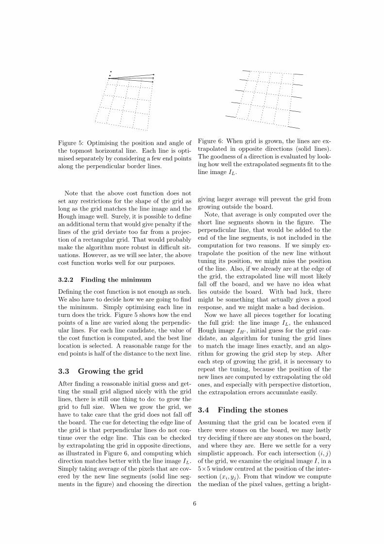
Figure 5: Optimising the position and angle ofthe topmost horizontal line. Each line is opti-mised separately by considering a few end pointsalong the perpendicular border lines.

Note that the above cost function does notset any restrictions for the shape of the grid aslong as the grid matches the line image and theHough image well. Surely, it is possible to definean additional term that would give penalty if thelines of the grid deviate too far from a projec-tion of a rectangular grid. That would probablymake the algorithm more robust in difficult sit-uations. However, as we will see later, the abovecost function works well for our purposes.

3.2.2 Finding the minimum

Defining the cost function is not enough as such.We also have to decide how we are going to findthe minimum. Simply optimising each line inturn does the trick. Figure 5 shows how the endpoints of a line are varied along the perpendic-ular lines. For each line candidate, the value ofthe cost function is computed, and the best linelocation is selected. A reasonable range for theend points is half of the distance to the next line.

3.3 Growing the grid

After finding a reasonable initial guess and get-ting the small grid aligned nicely with the gridlines, there is still one thing to do: to grow thegrid to full size. When we grow the grid, wehave to take care that the grid does not fall offthe board. The cue for detecting the edge line ofthe grid is that perpendicular lines do not con-tinue over the edge line. This can be checkedby extrapolating the grid in opposite directions,as illustrated in Figure 6, and computing whichdirection matches better with the line image IL.Simply taking average of the pixels that are cov-ered by the new line segments (solid line seg-ments in the figure) and choosing the direction

Figure 6: When grid is grown, the lines are ex-trapolated in opposite directions (solid lines).The goodness of a direction is evaluated by look-ing how well the extrapolated segments fit to theline image IL.

giving larger average will prevent the grid fromgrowing outside the board.

Note, that average is only computed over theshort line segments shown in the figure. Theperpendicular line, that would be added to theend of the line segments, is not included in thecomputation for two reasons. If we simply ex-trapolate the position of the new line withouttuning its position, we might miss the positionof the line. Also, if we already are at the edge ofthe grid, the extrapolated line will most likelyfall off the board, and we have no idea whatlies outside the board. With bad luck, theremight be something that actually gives a goodresponse, and we might make a bad decision.

Now we have all pieces together for locatingthe full grid: the line image IL, the enhancedHough image IH′ , initial guess for the grid can-didate, an algorithm for tuning the grid linesto match the image lines exactly, and an algo-rithm for growing the grid step by step. Aftereach step of growing the grid, it is necessary torepeat the tuning, because the position of thenew lines are computed by extrapolating the oldones, and especially with perspective distortion,the extrapolation errors accumulate easily.

3.4 Finding the stones

Assuming that the grid can be located even ifthere were stones on the board, we may lastlytry deciding if there are any stones on the board,and where they are. Here we settle for a verysimplistic approach. For each intersection (i, j)of the grid, we examine the original image I, in a5×5 window centred at the position of the inter-section (xi, yj). From that window we computethe median of the pixel values, getting a bright-

6

ness value B(i, j). For each intersection, we alsocompute the median of the brightness values ina local 5× 5 neighbourhood: M(i, j). Then thestones S(i, j) can be decided as follows:

S(i, j) =

white if B(i,j)M(i,j) > T,

black if M(i,j)B(i,j) > T,

empty otherwise.

(7)

A good value for the threshold T can be deter-mined empirically. We will set T to 1.2 for now.

4 Tests and discussion

4.1 Tests

The system described above was implemented inMATLAB.1 Figures 7–12 show six test imagesdemonstrating how the system works. In eachfigure, the original image is shown at top, andthe analysis of the system is shown below. Thewhite stones are marked with circles and blackstones with asterisks. The images in Figures 7–10 have been analysed correctly, one black stonehas been missed in Figure 11, and Figure 12shows an image on which the system failed, be-cause it could not find sensible initial lines fromthe Hough image, shown also in the figure.

4.2 Problems in detecting lines

As can be seen from the test images, the systemfinds the playing grid quite well even if there aresome stones on the board, as long as the mostof the lines are visible. Also, low viewing an-gles are tolerated. Figure 12 shows perhaps thebiggest weakness of the current approach. Theanalysis fails simply because there are too manystones obscuring the centre lines. The peaks intoHough image are too weak and the algorithmfails to find them.

There are a few techniques that might im-prove the Hough image. If the local line di-rections were estimated for each pixel in theline image IL, the information could be takeninto account in the Hough transform, so thatonly part of the array cells need to be up-dated [Sonka et al., 1998, pp. 169]. That wouldprobably reduce the noise in the Hough im-age. There are also many variations and ex-tensions of the Hough transform presented in

1The source code of the system is available for down-load at http://www.cis.hut.fi/thirsima/gocam/

the literature, that might be more robust tonoise. See, for example, the survey given in[Kälviäinen et al., 1995].

Whatever method for finding lines is used, thelines can not be found if the board is completelycovered by the stones. Considering the end ap-plication, if we can assume that the board andthe camera are not moving during the game, itis enough to locate the grid in the beginning ofthe game and perhaps to only fine tune grid dur-ing the game. However, if the application shouldtolerate moving of the camera, an analysis basedon finding stones would be needed.

4.3 Problems in detecting stones

In Figure 11, for example, we see that thestones are seldom located exactly at the inter-sections. Because the stones are lens shaped,and their thickness can be even half of theirradius, the centres of the stones are elevatedfrom the board. Additionally, the stones mighthave been placed carelessly off the intersections,which can make the effect even stronger. Thecurrent procedure for finding stones is quite sim-ple, but seems to work well enough for the testimages. It might be possible to try finding thecentre of the stone before analysing the colourof stone from a small window, but then it shouldbe decided if there is a stone on the intersectionin the first place.

The other difficulty in detecting stones isthat the lighting conditions can vary in differ-ent parts of the board. For this reason, try-ing to set simple threshold values for white andblack stones is not very robust. The intensityof the board surface on a brighter part may bequite close to the intensity of the white stonesin a darker part. Also, black stones may havesurprisingly bright reflections from lamps abovethe board. The current median based analysisseems to be quite robust, but assumes that thereare not too many stones of one colour in the lo-cal neighbourhood. The most straightforwardway to improve the stone detection algorithm isprobably to use colour images instead of gray-scale images.

4.4 From still images to video

So far we have analysed only still images, but inthe end application which would analyse videostream, it would probably be useful to analyseconsecutive frames, too, in order to detect if

7

Figure 7: Test image 1 (320×240): Top: The original image. Bottom: The analysis of the system.Black stones are marked with asterisks, white stones with circles.

8

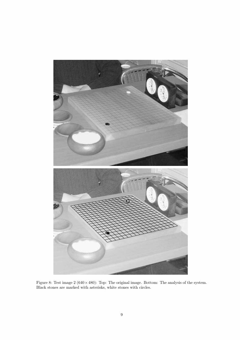
Figure 8: Test image 2 (640×480): Top: The original image. Bottom: The analysis of the system.Black stones are marked with asterisks, white stones with circles.

9

Figure 9: Test image 3 (350×280): Top: The original image. Bottom: The analysis of the system.Black stones are marked with asterisks, white stones with circles.

10

Figure 10: Test image 4 (440 × 373): Top: The original image. Bottom: The analysis of thesystem. Black stones are marked with asterisks, white stones with circles.

11

Figure 11: Test image 5 (790 × 600): Top: The original image. Bottom: The analysis of thesystem. Black stones are marked with asterisks, white stones with circles.

12

Angle (θ)

Dis

tanc

e (ρ

)

0 50 100 150

−300

−200

−100

0

100

200

300

Figure 12: Test image 6 (650×522): Top: The original image, which the system could not analysecorrectly. Bottom: The Hough image.

13

the colour around each intersection has changed.Also, it is perhaps not necessary to do the fullprocedure of finding lines and stones for everyframe, if it can be assumed that the board andthe camera do not move much during the record-ing. Then a separate fast analysis would be nec-essary to decide if the position on the board haschanged. Also, the system should be able to de-cide if it is worthwhile to analyse the positionat all. When a player is placing a stone on theboard, the board is partly obscured.

5 Conclusion

All in all, the presented system for analysingphotos of go boards and reading the position onthe board seems to work well. It finds the gridlines using linear filtering and Hough transform,and is quite robust if there are not too manystones on the board. Also, the colours of thestones can be decided quite well. The currentsystem is only able to analyse still images, butextending the system to analyse videos of com-plete go games seems possible.

References

[Kälviäinen et al., 1995] Kälviäinen, H., Hirvo-nen, P., Xu, L., and Oja, E. (1995). Prob-abilistic and non-probabilistic Hough trans-forms: overview and comparisons. Image and

Vision Computing, 13(4):239–315.

[Sonka et al., 1998] Sonka, M., Hlavac, V., andBoyle, R. (1998). Image Processing, Analysis,

and Machine Vision. International ThomsonPublishing Inc., 2nd. edition.

14