Extracting information from S-curves of language change

Fakhteh Ghanbarnejad,1, ∗ Martin Gerlach,1, ∗ Jose M. Miotto,1 and Eduardo G. Altmann1, †

1Max Planck Institute for the Physics of Complex Systems, Dresden,Germany

I. DATA

The data for the timeseries is obtained from the latest version of the google-ngram database [1], which is anextension of the original data [2] enriched with more data and syntactic annotations. Given two or three linguisticvariants, denoted by q = 1, 2 or 3, we count the total number of occurrences of each variant by nq(t) in each yeart ∈ [1800, 2008] irrespective of its capitalization. From this we estimate the fraction of adopters ρ(t) by the relativeusage of variant ’1’ for the given word (w):

ρw(t) =nw1 (t)∑q n

wq

. (1)

Figures ?? show S-curves of individual words. We calculate the average relative usage of one variant as an averageover all tockens of the ensemble, i.e.

ρavg(t) =

∑w n

w1∑

w

∑q n

wq

. (2)

The relative frequency of a word, f relw (t), is measured as the relative weight of both (or the three) variants combined:

f relw (t) =

∑q n

wq (t)∑

w

∑q n

wq (t)

(3)

While the frequency of a word, fw(t), is measured as the weight of all the variants combined divided by the size ofthe database (in word tokens):

fw(t) =

∑q n

wq (t)

#tokens in the corpus at yeart(4)

We associate an error σρ(t) to each datapoint (t, ρ(t)), which we split into two parts, i.e.

σ2ρ = σ2

s + σ20 (5)

in which σs is due to finite sampling of the data, and σ0 subsumes additional uncertainties from exogenous perturba-tions. The introduction of the latter is necessary, because only considering the finite-sampling effect does not accountfor the observed fluctuations in the frequency of the most common words, which we assume to be stationary.

The effect of finite sampling, σs, is approximated by assuming that n1 and n2 (q = 1, 2) are the outcomes of abinomial process with n = n1 + n2 samples where variant ’1’ is drawn with probability p = n1/N and variant ’2’ isdrawn with probability 1− p. From this we can calculate the error σs:

σs(t)2 =

n1(t)n2(t)

(n1(t) + n2(t))3 . (6)

For the estimation of σ0, which we treat as constant and independent of the sample size n(t) = n1(t)+n2(t) in eachyear, we look at the timeseries of the relative frequency of the most frequent word, "the", in the English language.Assuming that this timeseries is stationary, we estimate σ0, such that 95% of the points of the timeseries lie withinthe 95% confidence-interval assuming Gaussian errors according to Eq. (5). This gives σ2

0 = 0.002, which we use inall cases.

∗Both authors contributed equally to this work.†Electronic address: {fakhteh,gerlach,jmiotto,edugalt}@pks.mpg.de

2

A. German orthographic reforms

In this section we focus exclusively on the competition between the letters ’ß’ (s-sharp, q = 2) and ’ss’ (q = 1)encoding the sound for voiceless s in the German orthography. The official set of rules concerning the usage of eachvariant was changed twice in the orthographic reforms of 1901 and 1996 [3]. We investigate the usage of each variantover time for 2960 words as being affected by the orthographic reform of 1996 [4]. We consider the timeseries of fourrepresentative cases: (i) ρavg(t); and three individual words as the most frequent (ii) word ’dass’, ρdass(t); (iii) verb’muss’, ρmuss(t); and (iv) noun ’einfluss’, ρeinfluss(t).

B. Russian Names

In this section we focus on two Russian name-suffixes: ’ов’ and ’ев’. The letter ’в’ has been written in Romanscript languages like English (en) and German (de) by ’v’, ’w’ or ’ff’. Here we consider the competition between theletter ’v’ (q = 1) and two others together ’w’+’ff’ (q = 2 and q = 3); while all the official standard systems suggest ’v’for ’в’. We investigate the usage of each variant over time for 50 common Russian names which are listed below. Wepresent the timeseries of six representative cases: (i) the average over all words, ρavg(t); (ii) the five most used wordsρw(t).

a. German: Charkov, Saratov, Romanov, Stroganov, Tambov, Pirogov, Godunov, Katkov, Aksakov, Demidov,Semenov, Lermontov, Saltykov, Kornilov, Stepanov, Lobanov, Bulgakov, Krylov, Melnikov, Annenkov, Turgenev,Kostomarov, Filatov, Grekov, Putilov, Titov, Vinogradov, Danilov, Sobolev, Nikiforov, Kamenev, Novikov, Kondakov,Martynov, Rykov, Melikov, Platonov, Karpov, Lazarev, Balabanov, Krasnov, Nabokov, Dolgorukov, Kirov, Leonov,Maklakov, Naumov, Frolov, Mitrofanov, Fedotov

b. English: Saratov, Demidov, Pirogov, Tambov, Charkov, Katkov, Kornilov, Lazarev, Novikov, Melikov, Ler-montov, Aksakov, Godunov, Turgenev, Menshikov, Stepanov, Vinogradov, Semenov, Kutuzov, Lebedev, Suvorov,Lomonosov, Mendeleev, Lavrov, Melnikov, Lobanov, Annenkov, Volkhov, Balakirev, Lvov, Bazarov, Shuvalov, Grig-oriev, Titov, Yakov, Nekrasov, Mikhailov, Gorchakov, Morozov, Zubov, Chekhov, Sakharov, Dragomirov, Andreyev,Danilov, Chirikov, Yermolov, Bulgakov, Vasiliev, Saltykov

To make this lists, the primary list of common Russian names ending ’ов’ and ’ев’ was created according to theEnglish Wikipedia pages including: List of surnames in Russia, List of Russian-language writers, scientists, composers,leaders of the Soviet Union and Marshal of the Soviet Union; Also list of cities and towns in Russia was counted inthis list. The words which have been used at least a) one time between 1800 and 2008 and b) 10 times for more than100 years (75 years for German data) in this period were included in the initial list. Then in order to guarantee thatthese words are right competitors, we removed words satisfiying one of the following condistions:

• The words whose first letter were written mostly by small letters instead of capital letters (∑2008

t=1800 fsmallw (t)∑2008

t=1800 fcaptalw (t)

≥0.01)

• The names like Gorbachev which has a sudden peak at late 20 century and before that were rarely used(

∑2000t=1950 fword(t)

0.99∗∑2000

t=1850 fword(t)≥ 1)

• The names which have entries in Wikipedia not corresponding to the Russian origin e.g. Rostow which refersto Americans and Romanow which refers to Polish places

C. Regularization verbs in English

In this section we focus on the regularization of English verbs [5]. In addition to the regular past form of a verb, whichis generated by adding -ed (laugh → laughed), there exists a small number of verbs which are conjugated irregularly,e.g. burn → burnt. However, all irregular forms coexist with a corresponding regular variant [2]. We investigate thecompetition between the regular (q = 1) and the irregular (q = 2) form for 281 verbs with a recently attested irregularform [2]. As an example, for the verb ’write’, n1(t) = n(writed, t), and n2(t) = n(writ, t) + n(written, t) + n(wrote, t),since we have to combine the usage of past participle and preterit to capture all irregular past forms.

The following filtering is employed. We discarded any verb, where the irregular past form is the same as theinfinitive since it would not be possible to distinguish between a verb that is used as a past form or a present form,e.g. for the verb ’beat’ the irregular preterit is ’beat’. We condition the counts on those forms that are identified asverbs by the associated part-of-speech tags. We then selected the 10 verbs that exhibit the largest relative change

3

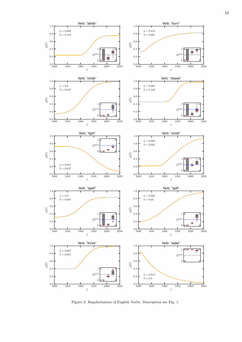
| ρ1 − ρ0 |, where ρ0 and ρ1 is the average over the 20 datapoints in the beginning (t ∈ [1800 − 1819]) and the end(t ∈ [1989− 2008]) of the timeseries respectively. These verbs are: abide (abided/abode), burn (burned/burnt), chide(chided/chid,chidden), cleave (cleaved/clove,cloven), light (lighted/lit), smell (smelled/smelt), spell (spelled/spilt),spill (spilled/spilt), thrive (thrived/throve,thriven), wake (waked/woke,waken).

II. SURROGATE DATA

In the following we describe how to apply our notion of endogenous and exogenous influence to several paradigmaticmodels of innovation spreading on complex networks.

A. Approximate Master Equation

We formulate the dynamics in the framework of approximate master equations (AME) [6], which describe thestochastic binary dynamics in an uncorrelated network with a given degree distribution Pk. Nodes can either bepotential adopters (susceptible) or have already adopted the innovation (infected) and are grouped into classes {k,m},where k denotes the degree and m the number of infected neighbors. The dynamics is specified by the function Fk,m(Rk,m), the rate at which susceptible (infected) {k,m}-nodes become infected (susceptible). In this work we onlyconsider monotone dynamics, i.e. Rk,m = 0, which leads to the following system of ordinary differential equations forthe fraction of susceptible {k,m}-nodes, sk,m:

d

dtsk,m =− Fk,msk,m − C (k −m) sk,m

+ C (k −m+ 1) sk,m−1, (7)

with C = 〈(k −m)Fk,msk,m〉/〈(k −m) sk,m〉 where 〈· 〉 =∑k Pk

∑km=0. From sk,m(t) we can calculate the timeseries

for the total fraction of infected nodes, ρ(t), according to:

ρ(t) = 1−∑k

Pk

k∑m=0

sk,m. (8)

Assuming that at time t0 a randomly chosen fraction of nodes, ρ(t0) = ρ0, is infected, we get as initial conditions forsk,m [6]:

sk,m(t0) =

(k

m

)ρm0 (1− ρ0)

k−m(1− ρ0) . (9)

We investigate two special cases of functions Fk,m with two parameters a and b:Bass-Model: In the Bass-model the probability of becoming infected is proportional to the number of neighbors

that are already infected:

Fk,m = a+ bm

k, (10)

Threshold-model: In a threshold-model a node becomes infected with probability 1 if the fraction of infectedneighbors exceeds a certain threshold:

Threshold: Fk,m =

{a, m/k < 1− b1, m/k ≥ 1− b . (11)

B. Exogenous and Endogenous Influence

The formulation of the spreading dynamics in the framework of AME allows us to calculate exactly the ’groundtruth’ of the exogenous and endogenous contributions for any given Fk,m. Following the approach in Sec. II, main

4

text, we can now calculate exactly the individual contributions:

Gj =1

N

N∑i=1

gj (t∗i )

g (t∗i ),

=1

N

∑k

∑i∈{k}

gj (t∗i ,m∗i , k)

g (t∗i ,m∗i , k)

,

=∑k

Pk

k∑m=0

∫ ∞0

gj (t,m, k)

g (t,m, k)∆k,m (t) dt, (12)

where ∆k,m(t) = Fk,msk,m is the actual fraction of {k,m}-nodes that changed from susceptible to infected at time t.Noting that the total rate of change is given by g(k,m) = Fk,m, it follows that

Gj =∑k

Pk

k∑m=0

∫ ∞0

gj (t,m, k) sk,m (t) dt, (13)

Assuming that the exogenous contribution is given by transitions that occur when no neighbor is infected, i.e.gexo (k,m) = Fk,0, the exogenous and endogenous contribution yields:

Gexo =∑k

Pk

k∑m=0

∫ ∞0

Fk,0sk,mdt,

Gendo =∑k

Pk

k∑m=0

∫ ∞0

(Fk,m − Fk,0) sk,mdt. (14)

C. Numerical Implementation

Given a degree-sequence k ∈ [kmin, kmax], a degree-distribution Pk, and one of the Fk,m from Eqs. (10,11), wecan solve the set of differential equations for sk,m numerically according to Eq. (7). We use scipy’s [7] odeint-implementation to get the timeseries ρ(t) from Eq. (9) and the true exogenous and endogenous influence from Eq. (14)for a particular trajectory. We set as parameters ρ0 = ρ(t0 = 0) = 10−3 and sample the trajectory ρ(t) at discretepoints t ∈ {t0 + i · dt} for i = 1, . . . , N with dt = 0.01 and ρ(t = Ndt) ≥ 1− ρ0.

III. FITTING METHODS

In this section we explore three different methods of how to quantitatively assess the endogenous and exogenousfactor in the spreading dynamics of a linguistic variant within the population. We want to restrict ourselves to theanalysis of the timeseries of the total fraction of adopters of the innovation, ρ(t), with ρ ∈ [0, 1] given a set of Nobservations D = {ti, ρi σi} with i = 1, . . . , N , where ti is the time, ρi the relative usage of one variant over the other,and σi the error associated to ρi, for details in the real data, see Sec. I

Our starting point for all three methods is the assumption that the dynamics of the total fraction of adopters, ρ(t),can be effectively described by a generalized population-dynamics model:

d

dtρ(t) = [1− ρ (t)] g (ρ (t)) , (15)

which means that the rate of change of ρ is determined by an arbitrary function g(ρ) only affecting the fraction ofsusceptibles, 1 − ρ. Further, we want to account for the fact that the fraction of adopters is bounded by the twoasymptotic values y0 and y1 such that ρ(t→ −∞) = y0 and ρ(t→∞) = y1, which gives for the dynamics

d

dtρ(t) =

{[y1 − ρ] g (ρ) , ρ ∈ [y0, y1]

0, else. (16)

This rescaling of the asymtoyics is necessary to compare the models (in which y0 = 0 and y1 = 1) to data (in whichtypically y0 > 0 and y1 < 1). Additional parameter t0 sets the characteristic timescale, such that ρ(t0) = 1

2 (y0 + y1),

5

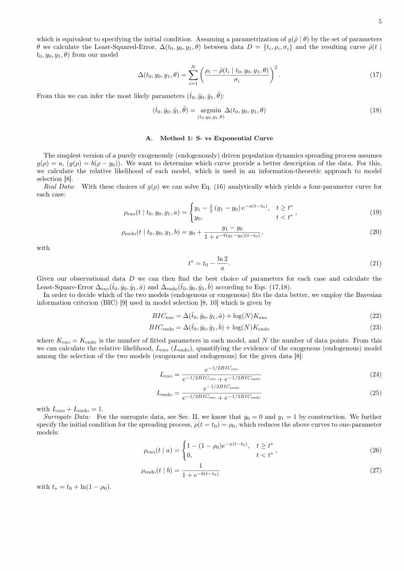
which is equivalent to specifying the initial condition. Assuming a parametrization of g(ρ | θ) by the set of parametersθ we calculate the Least-Squared-Error, ∆(t0, y0, y1, θ) between data D = {ti, ρi, σi} and the resulting curve ρ(t |t0, y0, y1, θ) from our model

∆(t0, y0, y1, θ) =

N∑i=1

(ρi − ρ(ti | t0, y0, y1, θ)

σi

)2

. (17)

From this we can infer the most likely parameters (t0, y0, y1, θ):

(t0, y0, y1, θ) = argmin(t0,y0,y1,θ)

∆(t0, y0, y1, θ) (18)

A. Method 1: S- vs Exponential Curve

The simplest version of a purely exogenously (endogenously) driven population dynamics spreading process assumesg(ρ) = a, (g(ρ) = b(ρ − y0)). We want to determine which curve provide a better description of the data. For this,we calculate the relative likelihood of each model, which is used in an information-theoretic approach to modelselection [8].

Real Data: With these choices of g(ρ) we can solve Eq. (16) analytically which yields a four-parameter curve foreach case:

ρexo(t | t0, y0, y1, a) =

{y1 − 1

2 (y1 − y0) e−a(t−t0), t ≥ t∗y0, t < t∗

, (19)

ρendo(t | t0, y0, y1, b) = y0 +y1 − y0

1 + e−b(y1−y0)(t−t0), (20)

with

t∗ = t0 −ln 2

a. (21)

Given our observational data D we can then find the best choice of parameters for each case and calculate theLeast-Square-Error ∆exo(t0, y0, y1, a) and ∆endo(t0, y0, y1, b) according to Eqs. (17,18).

In order to decide which of the two models (endogenous or exogenous) fits the data better, we employ the Bayesianinformation criterion (BIC) [9] used in model selection [8, 10] which is given by

BICexo = ∆(t0, y0, y1, a) + log(N)Kexo (22)

BICendo = ∆(t0, y0, y1, b) + log(N)Kendo (23)

where Kexo = Kendo is the number of fitted parameters in each model, and N the number of data points. From thiswe can calculate the relative likelihood, Lexo (Lendo), quantifying the evidence of the exogenous (endogenous) modelamong the selection of the two models (exogenous and endogenous) for the given data [8]:

Lexo =e−1/2BICexo

e−1/2BICexo + e−1/2BICendo(24)

Lendo =e−1/2BICendo

e−1/2BICexo + e−1/2BICendo(25)

with Lexo + Lendo = 1.Surrogate Data: For the surrogate data, see Sec. II, we know that y0 = 0 and y1 = 1 by construction. We further

specify the initial condition for the spreading process, ρ(t = t0) = ρ0, which reduces the above curves to one-parametermodels:

ρexo(t | a) =

{1− (1− ρ0)e−a(t−t0), t ≥ t∗0, t < t∗

, (26)

ρendo(t | b) =1

1 + e−b(t−t0)(27)

with t∗ = t0 + ln(1− ρ0).

6

B. Method 2: Mixed Curve

In this section we want to extend our previous model by assuming that, both, exogenous and endogenous drivingis present in the spreading dynamics simultaneously, i.e. g(ρ) = a+ b (ρ− y0).

Real Data: Solving Eq. (16) yields a 5-parameter curve for ρ:

ρmixed(t | t0, y0, y1, a, b) =

{−(a−by0)(y1−y0)+y1(2a+b(y1−y0))e[a+b(y1−y0)](t−t0)

b(y1−y0)+(2a+b(y1−y0))e[a+b(y1−y0)](t−t0) , t ≥ t∗y0, t < t∗

, (28)

with

t∗ = t0 −ln(2 + b

a (y1 − y0))

a+ b (y1 − y0). (29)

We note that the special case a = 0 yields t∗ → −∞, which means that for all finite t: ρ(t) > y0 and only in the limitρ(t→ −∞) = y0. Given the data D we estimate the most likely parameters (t0, y0, y1, a, b) using Eqs. (17,18).

For the given choice of g(ρ) = a+ (b− y0)ρ we define the exogenous and the endogenous influence as

gexo(ρ) = g(ρ = y0) = a, (30)

gexo(ρ) = g(ρ)− gexo(ρ) = b(ρ− y0). (31)

From this we can calculate the total exogenous and endogenous influence in the spreading process as the fraction ofthe population that switches at time t, ρ(t), weighted by the relative exogenous influence, gext(ρ)/g(ρ), and relativeendogenous influence, gint(ρ)/g(ρ), respectively, integrated along the complete trajectory ρ(t)

Gexo =1

y1 − y0

∫ ∞−∞

dtρ(t)gexo(ρ(t))

g(ρ(t))(32)

=1

y1 − y0

∫ y1

y0

dρgexo(ρ)

g(ρ)(33)

=1

y1 − y0

∫ y1

y0

dρa

a+ b (ρ− y0)(34)

=1

y1 − y0

a

bln

[a+ b (y1 − y0)

a

](35)

and

Gendo =1

y1 − y0

∫ ∞−∞

dtρ(t)gendo(ρ(t))

g(ρ(t))(36)

=1

y1 − y0

∫ y1

y0

dρgendo(ρ)

g(ρ)(37)

=1

y1 − y0

∫ y1

y0

dρb (ρ− y0)

a+ b (ρ− y0)(38)

= 1− 1

y1 − y0

a

bln

[a+ b (y1 − y0)

a

], (39)

in which we choose the prefactor 1/(y1 − y0) such that we have the normalization Gexo +Gendo = 1.Surrogate Data: For the surrogate data, see Sec. II, we know that y0 = 0 and y1 = 1 by construction. We

further specify the initial condition for the spreading process, ρ(t = t0) = ρ0, which reduces the above curve to atwo-parameter model:

ρmixed(t | a, b) =

{−a(1−ρ0)+(a+bρ0)e(a+b)(t−t0)

b(1−ρ0)+(a+bρ0)e(a+b)(t−t0) , t ≥ t∗0, t < t∗

, (40)

with

t∗ = t0 +1

a+ blna (1− ρ0)

a+ bρ0. (41)

7

C. Method 3: Nonparametric Curve

In this section we want to infer the exogenous and the endogenous influence non-parametrically not assuming anyspecific functional form of g(ρ). The idea is to infer g(ρ) from the timeseries directly according to Eq. (16)

g(ρ) :=ρ(t)

y1 − ρ(t). (42)

From this we can infer the exogenous and the endogenous influence along the trajectory ρ:

gexo = g(ρ = y0) (43)

gendo = g(ρ)− g(ρ = y0) (44)

which gives for the total exogenous and endogenous contribution

Gexo =1

y1 − y0

∫dρgextg(ρ)

(45)

Gendo =1

y1 − y0

∫dρgintg(ρ)

(46)

Surrogate Data: For the surrogate data we can infer g(ρ) directly with the timeseries ρ(t) being sampled at a givenresolution in discrete time, t = (ti) with i = 1..N , such that we can approximate the time-derivate of ρ(t) by finitedifferences, e.g.

ρ(ti) ≈ρ(ti+1)− ρ(ti)

ti+1 − ti(47)

for i = 1...N − 1. Assuming that ρ(t) is a monotone function in t, i.e. t = t(ρ), we can express the time derivative as

ρ(t)t=t(ρ)−→ ρ(ρ) (48)

such that we can evaluate g(ρ), see Eq. (42), from the timeseries ρ(t) and its derivative ρ via:

g(ρ) :=ρ [t(ρ)]

1− ρ (49)

Real Data: Real data is only available with a given resolution in t and is subject to fluctuations, therefore thedirect calculation of ρ in Eq. (42) does not lead to meaningful results. Instead, we want to infer g(ρ) indirectly, i.e.find a particular choice of g(ρ) that yields the best description of the data by solving Eq. (16) for ρ(t) and thenapplying Eqs. (17,18). Our approach is to parametrize g(ρ) by means of a natural cubic spline s(ρ) [10]. Therefore,we divide the support of g(ρ), ρ ∈ [y0, y1], into n intervals of equal length h = y1−y0

n , {[y0 + (i − 1)h, y0 + ih} fori = 1...n. In each interval i we define a cubic polynomial, such that the resulting curve sn(ρ) is piecewise-polynomialof order 4 and has continuous derivatives up to order 2. Furthermore, we restrict ourselves to natural cubic splineswhich implies that s′′n(ρ = y0) = s′′n(ρ = y1) = 0. The resulting spline sn(ρ) contains n+ 1 parameters θ = (θi) withi = 1...n+ 1 and two additional parameters (y0, y1) specifying the asymptotic values for ρ(t→ ±∞) which we denoteby sn(ρ | (y0, y1, θ)).

For any given n we can infer gn(ρ) = sn(ρ | y0, y1, θ) by Eqs. (16,17,18), which requires an extra parameter t0setting a characteristic time-scale of the change of ρ(t) in time. In total, for a parametrization of g(ρ) by a naturalcubic spline on n intervals, we have K = n + 4 parameters. Finally, the exogenous and the endogenous influence inthe spreading are calculated via Eqs. (43-46).

The crucial step then is to decide which value to choose for n as we have to find a trade-off between the mostaccurate description of the data and the problem of overfitting known as model selection [10]. We infer the best modelby means of the Bayesian information criterion (BIC), which penalizes models with additional parameters accordingto:

BIC = ∆ + log(N)K, (50)

where ∆ is the Least-Square error of the best fit of a given model according to Eqs. (17,18), K is the number ofparameters estimated, and N is the number of datapoints. Due to computational constraints we restrict ourselves tothe cases n = 1, ...10.

8

D. Numerical Implementation

The above mentioned methods require the minimization of the least-square error, see Eq. (18), in the space ofparameters (t0, y0, y1, θ). We find the most likely parameters (t0, y0, y1, θ) numerically using the ’L-BFGS-B’-algorithm[11] from scipy’s optimization package [7]. The algorithm allows to impose additional constraints on a parameter x,such that we ensure that xmin ≤ x ≤ xmax. In our case we choose the following constraints:

1. t0 is unconstrained,

2. 0 ≤ y0, y1 ≤ 1 since these parameters describe the asymptotic values of the fraction of adopters, i.e. ρ(t→ ±∞),

3. 0 ≤ a, b for method 1 and 2 considering positive exogenous and endogenous contributions,

4. 0 ≤ θi for i = 1, . . . , n+ 1 for method 3 in order to guarantee that g(ρ) ≥ 0.

Addressing the issue of local minima, for each timeseries we perform the minimization task 100 times with differentrandomly chosen initial conditions in parameter space and select the global minimum.

In Fig. 1-4 we show the individual timeseries from the data described in Sec. I, the best fit of the mixed curve,method 2 from Sec. III B, and the results for assessing the L and the exogenous factor, Gexo, from all three methods,Sec. III A-III C.

We calculate the confidence intervals from standard bootstrapping [10], i.e. performing the same analysis for anumber of B surrogate datasets obtained from random sampling with replacement of the original data (here B = 200).

9

1880 1890 1900 1910 1920 1930

t

0.0

0.2

0.4

0.6

0.8

1.0

ρ(t

)

a = 0.218

b = 0.0

ß −→ ss (1901): average

0

1

Gexo

1980 1990 2000 2010 2020 2030 2040 2050

t

0.0

0.2

0.4

0.6

0.8

1.0

ρ(t

)

a = 0.229

b = 0.0

ss −→ ß (1996): average

0

1

Gexo

1880 1890 1900 1910 1920 1930

t

0.0

0.2

0.4

0.6

0.8

1.0

ρ(t

)

a = 0.219

b = 0.0

ß −→ ss (1901): ”dass”

0

1

Gexo

1980 1990 2000 2010 2020 2030 2040 2050

t

0.0

0.2

0.4

0.6

0.8

1.0

ρ(t

)

a = 0.22

b = 0.0

ss −→ ß (1996): ”dass”

0

1

Gexo

1880 1890 1900 1910 1920 1930

t

0.0

0.2

0.4

0.6

0.8

1.0

ρ(t

)

a = 0.234

b = 0.0

ß −→ ss (1901): ”einfluss”

0

1

Gexo

1980 1990 2000 2010 2020 2030 2040 2050

t

0.0

0.2

0.4

0.6

0.8

1.0

ρ(t

)

a = 0.235

b = 0.039

ss −→ ß (1996): ”einfluss”

0

1

Gexo

1880 1890 1900 1910 1920 1930

t

0.0

0.2

0.4

0.6

0.8

1.0

ρ(t

)

a = 0.221

b = 0.0

ß −→ ss (1901): ”muss”

0

1

Gexo

1980 1990 2000 2010 2020 2030 2040 2050

t

0.0

0.2

0.4

0.6

0.8

1.0

ρ(t

)

a = 0.26

b = 0.0

ss −→ ß (1996): ”muss”

0

1

Gexo

Figure 1: Orthographic Reform of 1901 and 1996. The timeseries show the data (dots), the best fit of method 2 (line) with thevalues of its two parameters a and b, and the boxplot for the estimation of Gexo (inset) for all three methods: method 1 (left),method 2 (middle), and method 3 (right) with the result for the full data (red cross) and the 97.5%-, 75%-, 50%-,25%-, and2.5%- percentiles from bootstrapping (black lines).

10

1800 1850 1900 1950 2000 2050

t

0.0

0.2

0.4

0.6

0.8

1.0

ρ(t

)

a = 0.005

b = 0.119

Verb: ”abide”

0

1

Gexo

1800 1850 1900 1950 2000 2050

t

0.0

0.2

0.4

0.6

0.8

1.0

ρ(t

)

a = 0.012

b = 0.021

Verb: ”burn”

0

1

Gexo

1800 1850 1900 1950 2000 2050

t

0.0

0.2

0.4

0.6

0.8

1.0

ρ(t

)

a = 0.0

b = 0.047

Verb: ”chide”

0

1

Gexo

1800 1850 1900 1950 2000 2050

t

0.0

0.2

0.4

0.6

0.8

1.0

ρ(t

)

a = 0.001

b = 0.146

Verb: ”cleave”

0

1

Gexo

1800 1850 1900 1950 2000 2050

t

0.0

0.2

0.4

0.6

0.8

1.0

ρ(t

)

a = 0.001

b = 0.047

Verb: ”light”

0

1

Gexo

1800 1850 1900 1950 2000 2050

t

0.0

0.2

0.4

0.6

0.8

1.0

ρ(t

)

a = 0.006

b = 0.024

Verb: ”smell”

0

1

Gexo

1800 1850 1900 1950 2000 2050

t

0.0

0.2

0.4

0.6

0.8

1.0

ρ(t

)

a = 0.0

b = 0.087

Verb: ”spell”

0

1

Gexo

1800 1850 1900 1950 2000 2050

t

0.0

0.2

0.4

0.6

0.8

1.0

ρ(t

)

a = 0.001

b = 0.03

Verb: ”spill”

0

1

Gexo

1800 1850 1900 1950 2000 2050

t

0.0

0.2

0.4

0.6

0.8

1.0

ρ(t

)

a = 0.007

b = 0.072

Verb: ”thrive”

0

1

Gexo

1800 1850 1900 1950 2000 2050

t

0.0

0.2

0.4

0.6

0.8

1.0

ρ(t

)

a = 0.014

b = 0.0

Verb: ”wake”

0

1

Gexo

Figure 2: Regularization of English Verbs. Description see Fig. 1.

11

1800 1850 1900 1950 2000 2050

t

0.0

0.2

0.4

0.6

0.8

1.0

ρ(t

)

a = 0.0

b = 0.099

Russian -ov (en): average

0

1

Gexo

1800 1850 1900 1950 2000 2050

t

0.0

0.2

0.4

0.6

0.8

1.0

ρ(t

)

Russian -ov (en): ”charkov”

1800 1850 1900 1950 2000 2050

t

0.0

0.2

0.4

0.6

0.8

1.0

ρ(t

)

a = 0.07

b = 0.0

Russian -ov (en): ”demidov”

0

1

Gexo

1800 1850 1900 1950 2000 2050

t

0.0

0.2

0.4

0.6

0.8

1.0

ρ(t

)

a = 0.0

b = 0.14

Russian -ov (en): ”pirogov”

0

1

Gexo

1800 1850 1900 1950 2000 2050

t

0.0

0.2

0.4

0.6

0.8

1.0

ρ(t

)

a = 0.093

b = 0.0

Russian -ov (en): ”saratov”

0

1

Gexo

1800 1850 1900 1950 2000 2050

t

0.0

0.2

0.4

0.6

0.8

1.0

ρ(t

)

a = 0.107

b = 0.0

Russian -ov (en): ”tambov”

0

1

Gexo

Figure 3: Transliteration of Russian -ов (en). Description see Fig. 1.

12

1800 1850 1900 1950 2000 2050

t

0.0

0.2

0.4

0.6

0.8

1.0

ρ(t

)

a = 0.0

b = 0.078

Russian -ov (de): average

0

1

Gexo

1800 1850 1900 1950 2000 2050

t

0.0

0.2

0.4

0.6

0.8

1.0

ρ(t

)

a = 1.93

b = 0.308

Russian -ov (de): ”charkov”

0

1

Gexo

1800 1850 1900 1950 2000 2050

t

0.0

0.2

0.4

0.6

0.8

1.0

ρ(t

)

a = 0.03

b = 0.0

Russian -ov (de): ”romanov”

0

1

Gexo

1800 1850 1900 1950 2000 2050

t

0.0

0.2

0.4

0.6

0.8

1.0

ρ(t

)

a = 0.0

b = 0.654

Russian -ov (de): ”saratov”

0

1

Gexo

1800 1850 1900 1950 2000 2050

t

0.0

0.2

0.4

0.6

0.8

1.0

ρ(t

)

a = 0.0

b = 3.296

Russian -ov (de): ”stroganov”

0

1

Gexo

1800 1850 1900 1950 2000 2050

t

0.0

0.2

0.4

0.6

0.8

1.0

ρ(t

)Russian -ov (de): ”tambov”

Figure 4: Transliteration of Russian -ов (de). Description see Fig. 1.

13

[1] Yuri Lin, Jean-baptiste Michel, Erez Lieberman Aiden, Jon Orwant, Will Brockman, and Slav Petrov. Syntactic Anno-tations for the Google Books Ngram Corpus. In Proceedings of the ACL 2012 System Demonstrations, pages 169–174.Association for Computational Linguistics, 2012.

[2] Jean-Baptiste Michel, Yuan Kui Shen, Aviva Presser Aiden, Adrian Veres, Matthew K Gray, Joseph P Pickett, DaleHoiberg, Dan Clancy, Peter Norvig, Jon Orwant, Steven Pinker, Martin A Nowak, and Erez Lieberman Aiden. Quantitativeanalysis of culture using millions of digitized books. Science, 331(6014):176–182, 2011.

[3] Sally Johnson. Spelling trouble: Language, ideology and the reform of German orthography. Multilingual Matters, Clevedon,UK, 2005.

[4] Canoonet. German dictionaries and grammar [http://www.canoo.net]; accessed 03/04/2013.[5] Steven Pinker. Words and Rules: The Ingredients of Language. Basic Books, New York, NY, US, 1999.[6] James P. Gleeson. Binary-State Dynamics on Complex Networks: Pair Approximation and Beyond. Physical Review X,

3(2):021004, 2013.[7] Eric Jones et al. SciPy: Open source scientific tools for Python, 2001–.[8] K. P. Burnham and D. R. Anderson. Model Selection and Multimodel Inference: A Practical Information-Theoretic

Approach. Springer, 2nd ed. edition, 2002.[9] Gideon Schwarz. Estimating the Dimension of a Model. The Annals of Statistics, 6(2):461–464, 1978.

[10] Trevor Hastie, Robert Tibshirani, and Jerome Friedman. The Elements of Statistical Learning. Springer, 2nd edition,2009.

[11] R.H. Byrd, P. Lu, and J. Nocedal. A limited memory algorithm for bound constrained optimization. SIAM Journal onScientific and Statistical Computing, 16(5):1190–1208, 1995.