extracting topographic features from shuttle...

Technical Report, alg05-002 July 18, 2005

Wei-Wen Feng, [email protected] Peter Bajcsy, [email protected] National Center for Supercomputing Applications 605 East Springfield Avenue, Champaign, IL 61820 Extracting Topographic Features From Shuttle Radar

Topography Mission (SRTM) Images

Abstract This report addresses the problem of extracting topographic features from Shuttle Radar Topography Mission (SRTM) imagery. The features are used for Earth science applications and include slope, curvature, aspect, flow direction, flow accumulation and compound topographic index (CTI). The objective of our work is (1) to support topographic feature extraction similar to the one in ArcGIS, (2) to provide extraction of additional topographic features that are not supported in ArcGIS, (3) to increase statistical robustness of the extracted topographic features and (4) to let Earth science researchers use these algorithms by using the platform independent java code. We report (1) implementation details of each topographic feature, (2) accuracy comparisons of extracted features by I2K with the features extracted by ArcGIS, (3) differences in the extracted features as a function of statistical sample size, and (4) a summary of supported and unsupported topographic features in I2K and ArcGIS. Our results demonstrate that the results in I2K and ArcGIS software packages are almost identical. Furthermore, availability of additional topographic features and the flexibility of adjusting the feature extraction parameters are provided.

1 Introduction In order to learn about Earth science, it is desirable to extract topographic features of interest. The topographic features of interest in this report include slope, aspect, curvature, flow direction, flow accumulation and compound topographic index (CTI). These features can be extracted from digital elevation maps (DEM) and form an input into further analysis. Data mining systems can be then applied to discover relationships among multiple features.

In this report, we performed study with Shuttle Radar Topography Mission (SRTM) imagery acquired by NASA. The SRTM data corresponds to DEM data that can be combined with other NASA satellite data, e.g., MODIS or TERRA collections, for hydrological modeling purposes. The extraction process of topographic features from USGS DEM is the same as from NASA SRTM.

SRTM Feature Extraction

Feng, Bajcsy | Automated Learning Group, NCSA 2

We discuss both the theoretical definition and actual implementation of a topographic feature extraction process and compare our implementation with existing commercial package (ArcGIS). Our implementation is a component of Image To Knowledge (I2K) system developed in National Center of Supercomputing Application (NCSA). In the rest of the report, we will introduce the definition and implementation of these features in section 3 to 9, and compare the difference of our results with the results generated using the commercial package in section 10. In section 11, we will summarize relevant issues when computing these features from DEM data.

2 Terms and Definitions 2.1 Input Data: NASA SRTM and USGS DEM Shuttle Radar Topography Mission (SRTM) Images are composed of raster elevation data (see Figure 1). The data source of these images could be found at the corresponding NASA website (http://www2.jpl.nasa.gov/srtm). For each pixel in the image, there is a 16-bit elevation (height) value specified in meters and its geo-referencing information.

Topographic features are derived by applying specific algorithms to the input SRTM raster data. Each feature is represented by a raster image, where there might be one or more values assigned to each pixel depending on the type of a feature. In our experiments, we use SRTM data similar to the one shown in Figure 1 (16-bit short integer) for testing and accuracy evaluations. The extraction software developed also works with USGS DEM data set that are represented by 32-bit floating point numbers. 2.2 Software Packages: ArcGIS and I2K ArcGIS is a commercial GIS package developed by ESRI. It is the most widely used GIS software that is able to process and perform analysis on various GIS data formats. Image To Knowledge (I2K) is a library of tools developed at the National Center for Supercomputing Application (NCSA). I2K contains several capabilities and tools for geospatial raster and vector data integration, analysis and visualization.

Here, we compare our Java implementations of topographic feature extraction algorithms in the I2K system with ArcGIS implementations. In the following section, we refer our implementation as I2K and the commercial package as ArcGIS. 2.3 Image Processing: Pixel Neighborhood Definition Many topographic features are defined as partial derivatives of an elevation surface. While working with digital images, partial derivatives of continuous variables become finite differences of discrete spatial samples. The finite differences require considering a neighborhood of pixels (spatial samples) that are used for feature computation. Ideally, the spatial samples should be as close as possible to the estimated spatial location in order to achieve an accurate approximation of topographic features defined via partial derivatives (or small pixel neighborhood). However, for a fixed spatial resolution of a digital image, and in the presence of noise from measurements and analog-to-digital conversions, it is desirable to compute topographic features from as many samples as possible (or large neighborhood). These two conflicting objectives require exploring the size of a pixel neighborhood as a function of feature accuracy.



We use in all comparative experiments a 3 by 3 neighborhood for each pixel since that is the neighborhood size used in ArcGIS software. The notation of the neighborhood window is defined in Table 1. In I2K implementation, we also support different sizes of neighborhood windows to enhance the statistical robustness. Table 1: Neighborhood window definition.

3 SLOPE Slope is defined as the rate of elevation change in a cell’s 3 by 3 neighborhoods. Here we are interested in the degree angle of the slope as defined as the angle defined by rise (vertical distance change) and run (horizontal distance change), see Figure 2. For continuous case, it is obtained by computing the partial derivative components in x, y direction for each point. In practice, because DEM image is the discrete grid data, the derivative is computed using finite difference method in each cell’s neighborhood.



Figure 1: Original SRTM Data

3.1 ArcGIS implementation From the specification of ArcGIS, the slope implementation is defined as follow: rise_run = SQRT(SQR(dz/dx)+SQR(dz/dy)) degree_slope = ATAN(rise_run) *57.29578 where the deltas are calculated using a 3x3 roving window. For example: z1 through z9 represent the z_values in the window: (dz/dx) = ((z1 + 2*z4 + g) - (z3 + 2*z6 + z9)) / (8 * x_mesh_spacing)(dz/dy) = ((a + 2*z2 + z3) - (z7 + 2*z8 + z9)) / (8 * y_mesh_spacing)

Rise (Vertical distance change )

Run (Horizontal distance change)

S

Figure 2: Definition of slope as the angle from horizontal



3.2 I2K implementation

1 1

1 1

1 1

1 1

2 2

:( , ) ( , )

( , ) ~ ( 1, ) ( 1, ) ( 1, ) ( 1, ) /(8* )

( , ) ~ ( , 1) ( , 1) ( , 1) ( , 1) /(8* )

;

x y

x xi i

y yi i

x y

SlopeI x y I x ya a

x yI x y v I x y i I x y i I x y I x y res

x

I x y v I x i y I x i y I x y I x y resy

MagSlope v v AngleS

=− =−

=− =−

∂ ∂+

∂ ∂

∂= − + − + + + − − +

∂

∂= + − − + + + − − +

∂

= +

∑ ∑

∑ ∑

1tan ( )lope MagSlope−=

(1)

4 CURVATURE Curvature is a metric to measure the shape of the elevation. For an upward convex region, the curvature is positive, and negative for a concave region. It is obtained by computing the sum of the 2nd derivative of the I(x,y) with respect to both x,y direction [Zeverbergen 87]. In I2K implementation, we also compute the direction of the largest curvature as curvature angle, which is not supported by ArcGIS. 4.1 ArcGIS Implementation From the specification of ArcGIS, the curvature implementation is defined as follow: Calculates the curvature of a surface at each cell center. CURVATURE(<grid>, {out_profile_curve}, {out_plan_curve}, {out_slope}, {out_aspect}) Arguments <grid> - a grid representing a continuous surface. {out_profile_curve} - an optional output grid showing the rate of change of slope for each cell. This is the curvature of the surface in the direction of slope. {out_plan_curve} - An optional output grid showing the curvature of the surface perpendicular to the slope direction, referred to as the platform curvature. {out_slope} - An optional output grid showing the rate of maximum change in z value from each cell. This is the first derivative of the surface. {out_aspect} - An optional output grid showing the direction of the maximum rate of change in z value from each cell. This is also referred to as the slope direction.



Notes A positive curvature indicates that the surface is upwardly convex at that cell. A negative curvature indicates that the surface is upwardly concave at that cell. A value of zero indicates that the surface is flat. Units of the CURVATURE output grid as well as the units for the optional {out_profile_curve} and {out_plan_curve} output grids are one over 100 zunits, or 1/100(zunits). The reasonably expected values of all three output grids for a hilly area (moderate relief) may differ from about -0.5 to 0.5, while for the steep rugged mountains (extreme relief), the values may vary between -4 and 4. The units of {out_slope} are degrees. Values may vary from 0 to 90. Aspect is expressed in positive degrees from 0 to 359.9, measured clockwise from the north. An aspect value of -1 indicates an area of undefined aspect (i.e., flat). The direction of slope is defined by the value of aspect. Valid expressions include: outgrid = curvature(ingrid) outgrid = curvature(ingrid, helen_prof, helen_plan)outgrid = curvature(ingrid, #, #, helen_slope, helen_aspect) Discussion The curvature of a surface is calculated on a cell-by-cell basis. For each cell, a fourth-order polynomial of the form Z = Ax2y2 + Bx2y + Cxy2 + Dx2 + Ey2 + Fxy + Gx + Hy + I is fit to a surface composed of a 3x3 window. The coefficients a, b, c, and so on, are calculated from this surface. The relationships between the coefficients and the nine values of elevation for every cell numbered as shown on the diagram are as follows: A = [(Z1 + Z3 + Z7 + Z9) /4 - (Z2 + Z4 + Z6 + Z8) /2 + Z5] /L4 B = [(Z1 + Z3- Z7 - Z9) /4 - (Z2 - Z8) /2] /L3 C = [(-Z1 + Z3 - Z7 + Z9) /4 + (Z4 - Z6)]/2] /L3 D = [(Z4 + Z6) /2 - Z5] /L2 E = [(Z2 + Z8) /2 - Z5] /L2 F = (-Z1 + Z3 +Z7 - Z9) /4L2 G = (-Z4 +Z6) /2L H = (Z2 - Z8) /2LI = Z5 The output of the CURVATURE function is the second derivative of the surface (i.e., the slope of the slope), such that Curvature = -2(D + E) * 100 From an applied viewpoint, output of the CURVATURE function can be used to describe the physical characteristics of a drainage basin in an effort to understand erosion and runoff processes. The slope affects the overall rate of movement down slope. Aspect defines the direction of flow. The profile curvature affects the acceleration and deceleration of flow, and therefore influences erosion and deposition. The platform curvature influences convergence and divergence of flow. Examples



Displaying contours over a grid may help with the understanding and interpretation of the data resulting from the execution of the CURVATURE function. Grid: curvagrid = curvature(elevgrid, profileg, plang, slopeg, aspectg) Use LATTICECONTOUR to create contours of your grid: Arc: usage latticecontourUsage: LATTICECONTOUR <in_lattice> <out_cover> <interval>{base_contour} {contour_item}{weed_tolerance} {z_factor}Arc: latticecontour elevgrid elevcov 100 Arc: latticecontour slopeg slopecov 5Arc: gridGrid: image curvagridGrid: linecolor redGrid: arcs eleccovGrid: linecolor greenGrid: arcs slopecov 4.2 I2K implementation

2 2

2 2

2 1 1 1

21 1 1

2 1 1 1

21 1 1

:( , ) ( , )

( , ) 1 1 1~ ( 1, ) ( 1, ) 2 ( , )3 3 3

( , ) 1 1 1~ ( , 1) ( , 1) 2 ( , )3 3 3

x y

xi i i

yi i i

CurvatureI x y I x ya a

x yI x y v I x y i I x y i I x y i

x

I x y v I x i y I x i y I x i yy

MagCurvat

=− =− =−

=− =− =−

∂ ∂+

∂ ∂

∂ = − + + + + − + ∂ ∂

= + − + + + − + ∂

∑ ∑ ∑

∑ ∑ ∑

1( )*100; tan ( )yx y

x

vure v v AngleCurvature

v−= + =

(2)

Stored as ImageObject(numrows x numcols x 2 samples per pixel x DOUBLE type)= [Mag, Angle].



Figure 3 Curvature angle (Not supported in ArcGIS)

5 ASPECT Aspect identifies the down-slope direction of the maximum rate of change in value from each cell to its neighbors. It could be thought of as the angle between slope direction and the north direction. The angle is expressed in positive degrees from 0 to 360, measured clockwise starting at 0 from the north. 5.1 ArcGIS Implementation

From the specification of ArcGIS, the slope implementation is defined as follows: Aspect identifies the down-slope direction of the maximum rate of change in value from each cell to its neighbors. (Aspect can be thought of as the slope direction, but oddly enough, the slope is not used to compute aspect). The values of the output grid will be the compass direction of the aspect (expressed in positive degrees from 0 to 360, measured clockwise from the north). Cells in the input grid of zero slope (flat) are assigned an aspect of -1. If the input pixel has NODATA, the output is assigned NODATA. If any neighborhood cells are NODATA, they are assigned the value of the center cell in the computation of the aspect. The neighborhood is restricted to only the surrounding pixels.



5.2 I2K Implementation

1 1

1 1

1 1

1 1

1

:( , ) ( , )

( , ) ~ ( 1, ) ( 1, ) ( 1, ) ( 1, ) /(8* )

( , ) ~ ( , 1) ( , 1) ( , 1) ( , 1) /(8* )

tan ( )

x y

x xi i

y yi i

y

x

AspectI x y I x ya a

x yI x y v I x y i I x y i I x y I x y res

x

I x y v I x i y I x i y I x y I x y resy

vAspect

v

=− =−

=− =−

−

∂ ∂+

∂ ∂

∂= − + − + + + − − +

∂

∂= + − − + + + − − +

∂

=

∑ ∑

∑ ∑

(3)

6 FLOWDIRECTION: The direction of flow is determined by finding the direction of steepest descent from each cell [Greenlee 87]. We first calculate the drop in each 8 neighborhood as Drop = (ZDiff / Distance * 100). Here the ZDiff is the elevation difference between the center cell and its neighbor, and the Distance is defined as the distance between 2 cell centers. Note that the distances would be different between two orthogonal cells and two diagonal cells. The values for directions are power of 2 for each direction from the center, as used by ESRI flow direction encoding. The direction value start as 1 from east, and is multiplied by 2 as it changes clockwise, see Figure 4. For example, if the direction of steepest drop was to the left of the current processing cell, its flow direction would be coded as 16. For finding the steepest descent, there are some special cases need to be dealt with. If the descent to all adjacent cells is the same, then this cell is first marked as flat. Later in the second pass, the BFS (Breadth-First Search) algorithm is used to assign the flow direction to these flat cells. However, there would be some cases that one or more cells are identified as sinks because they are all lower than their surrounding neighborhoods. For this case, there is no feasible way to assign an outward flow direction to these cells. Thus a depression filling preprocessing is necessary to fill these pits before we could apply the flow direction computation. The detail procedure of depression filling could be found at Section 9. Our flow direction model uses the same definition of ArcGIS flow direction, though the actual implementation of flow computation including depression fill preprocessing follows the method proposed by [Lars 2002].



6.1 ArcGIS Implementation

From the specification of ArcGIS, the flow direction implementation is defined as follows: The direction of flow is determined by finding the direction of steepest descent from each cell. This is calculated as drop = change in z value / distance * 100. The output of FLOWDIRECTION is an integer grid whose values range from 1 to 255. The values for each direction from the center are encoded from 1 to 128. See Figure 4 ESRI Flow direction encoding for detail.

6.2 I2K Implementation The mathematical definition used for implementation in I2K is defined as the following formula.

32

16

8

64

4

128

1

2

Figure 4 ESRI Flow direction encoding



:

( , ) 1 ( , ) 1 ( , ) 1 ( , ) 1max , , ,( )

( , ) 1 ~ ( ( , ) ( , )) / ; 1,0,1

( , ) 1 ~ ( ( , ) ( , )) / ; 1,0,1

( ,

x y xy xyx y xy xy

x xx

y yy

Flow Direction

I x y I x y I x y I x ya a a ax y xy xy

I x y v I x i y I x y res ix

I x y v I x y j I x y res jy

I x

−−

∂ ∂ ∂ ∂ ∂ ∆ ∂ ∆ ∂ ∆ ∂ − ∆

∂= + − = −

∂ ∆∂

= + − = −∂ ∆

∂

{ }{ }

2 2

2 2

) 1 ~ ( ( , ) ( , )) / ; 1,0,1

( , ) 1 ~ ( ( , ) ( , )) / ; 1,0,1( )

min , , ,

(1) min , , ,

0{1,

xy x yxy

xy x yxy

x y xy xy

x y xy xy

y v I x i y i I x y res res ixy

I x y v I x i y i I x y res res ixy

If one v v v v then

MaxDrop v v v v and

MaxDropAngleFlowDir

−−

−

−

= + + − + = −∂ ∆

∂= − + − + = −

∂ − ∆

=

<=

1

2, 4,8,16,32,64,128}; ( 0) [ ~ 0; ]

(2) 0

(2 ) (min )

(2 ) ( ,1987)

numMin

ii

LUT MagFlowDir column clockwiseelse

if MagFlowDir then

a AngleFlowDir AngleFlowDir

elseb AngleFlowDir LUT Greenlee

=

> = +

≥

=

=

∑

(4)

7 FLOW ACCUMULATION: Flow accumulation is computed by accumulating the weight for all cells that flow into each down slope cell. For cells that have no incoming flows, the weights are 1. For those with incoming flows, the weight is 1 plus the sum of weight for each cell flowing into this cell. 7.1 ArcGIS Implementation

From the specification of ArcGIS, the flow accumulation implementation is defined as follows: Create a grid of accumulated flow to each cell by accumulating the weight for all cells that have flows into each downslope cell. The accumulated flow is based upon the number of cells flowing into each cell in the output grid. The current processing cell is not considered in this accumulation.

7.2 I2K implementation:



The algorithm for computing Flow Accumulation follows the steps below:

1. Identify all of the cells which have no incoming flows and mark them as “Source Cells” ( check its 8 neighbors to verify if there is any neighboring cell has flow direction into this cell. ).

2. For each “Source Cell”, trace the down flowing stream by following the flow direction to step toward the neighboring cell. For each step, add the current accumulation (Accum.) from previous cell plus 1 to the current cell’s flow accumulation. However, to avoid redundant accumulation, as soon as we enter a previously visited cell (check if its accumulation equals zero. If not, then it’s been visited. ), we only add the current accumulation to all the remaining down stream cells without plus 1 for each step.

3. Repeat 2, until there is no Source cell.

The pseudo code for this algorithm is:

<Identify Source cells >

For each Source cell do

Accum = 0.

Start at Source cell, set its accumulation to 0.

Find and step into next cell according to flow direction

While (not crossing boundary || is still a valid cell)

Add (Accum +1) to this cell’s accumulation.

If (this cell has not been visited)

Accum++

Find next cell according to flow direction in this cell

Step into next cell.

End while

End for each

8 COMPOUND TOPOGRAPHIC INDEX

The Compound Topographic Index (CTI), commonly referred to as the Wetness Index [Moore 91], is a function of the upstream contributing area (flow accumulation) and the slope of the landscape. It is not directly supported in ArcGIS implementation.



8.1 I2K Implementation

:ln( / tan( ))

Compound Topographic IndexCTI FlowAccum SlopeAngle=

(5)

Figure 5 I2K result of Compound Topographic Index (Not supported by ArcGIS)

9 Depression Filling: Because a DEM image is a discretization of the geography height value, there will exist both real pits from the original data or artificial pits results from noise during data acquisition. The presence of these pits will block the waterflow and cause the inaccurate or incorrect flow direction/accumulation. To resolve this issue, a depression filling preprocess is necessary before we compute any other features from the DEM image [Jenson 88]. The I2K implementation follows the method proposed in [Lars 2002]. The detailed procedure of filling the sink is described next.

9.1 Sink In the flow direction assignments, there would be some special cases where no flow directions could be assigned. Those are marked as flat areas in the flow direction image, and further processing is needed to resolve these cases.



If a flat area is a part of a larger plateau, it could be resolved by using a BFS (Breadth-First Search) method based on the method proposed by Lars Arge and his coworkers [Lars 2002] to assign appropriate flow directions. However, some flat areas are parts of sinks (see Figure 6), where no possible flow directions could be assigned before some special pre-processing is performed to fill the sinks. Although the sink detection result is part of the process in depression-filling, it could not be directly obtained in ArcGIS.

Figure 6 Sink detection result, the white pixels indicate the sink (Not supported by ArcGIS).

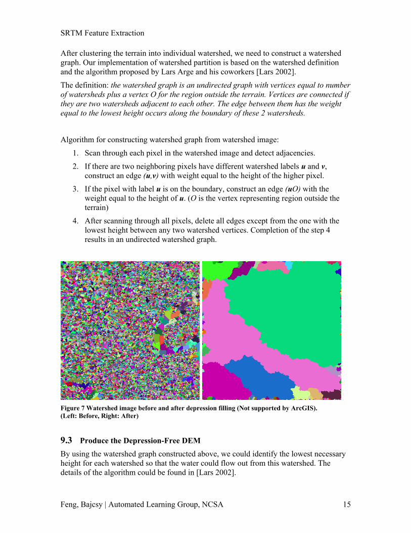
9.2 Watershed Watershed image forms a partition of the original image. The watershed feature, although it is an intermediate product of sink filling, could not be directly obtained from ArcGIS. First, a watershed algorithm clusters the pixels that will flow into the same sink together. Next, it will identify the outgoing path of each cluster to its adjacent watersheds (clusters). Finally, the algorithm lifts the sinks in a cluster to the lowest outgoing height of the cluster.



After clustering the terrain into individual watershed, we need to construct a watershed graph. Our implementation of watershed partition is based on the watershed definition and the algorithm proposed by Lars Arge and his coworkers [Lars 2002].

The definition: the watershed graph is an undirected graph with vertices equal to number of watersheds plus a vertex O for the region outside the terrain. Vertices are connected if they are two watersheds adjacent to each other. The edge between them has the weight equal to the lowest height occurs along the boundary of these 2 watersheds.

Algorithm for constructing watershed graph from watershed image:

1. Scan through each pixel in the watershed image and detect adjacencies.

2. If there are two neighboring pixels have different watershed labels u and v, construct an edge (u,v) with weight equal to the height of the higher pixel.

3. If the pixel with label u is on the boundary, construct an edge (uO) with the weight equal to the height of u. (O is the vertex representing region outside the terrain)

4. After scanning through all pixels, delete all edges except from the one with the lowest height between any two watershed vertices. Completion of the step 4 results in an undirected watershed graph.

Figure 7 Watershed image before and after depression filling (Not supported by ArcGIS). (Left: Before, Right: After) 9.3 Produce the Depression-Free DEM By using the watershed graph constructed above, we could identify the lowest necessary height for each watershed so that the water could flow out from this watershed. The details of the algorithm could be found in [Lars 2002].



Algorithm for filling depression from watershed graph:

1. Construct a flow directed graph F from the input watershed undirected graph by checking each edge (u,v) in the watershed graph and constructing a directed edge from u to v with weight S, if the edge (u,v) is the spill-elevation of u. (Note: a spill-elevation of a watershed u is the weight of the lightest edge in watershed graph incident to u).

2. For the case of a cyclical directional path (denoted as a cycle) in the flow directed graph F, contract the cycle by merging all watersheds in the same cycle into one, and compute the new spill-elevation edge in F

3. After processing each cycle in F, raise each remaining watershed u to the height of its spill-elevation height (The lightest edge incident to u). This is done by scanning all pixels belong to watershed u, and raise those pixels lower than spill-elevation.

Figure 8: Flow accumulation before and after depression filling. (Left: Before, Right: After)

10 ArcGIS and I2K Comparative Result

In this section we compute the topographic features from an SRTM image using both ArcGIS and I2K implementation and compare their differences. The testing image is the original SRTM data captured at N 38 W 78 with 1200 X 1200 image resolution. The specification of this SRTM format could be found at www.dlr.de/srtm/produkte/SRTM-XSAR-DEM-DTED-1.1.pdf . The results are discussed in the following sections. The detailed values of the average difference for each feature could be found in Table 2.



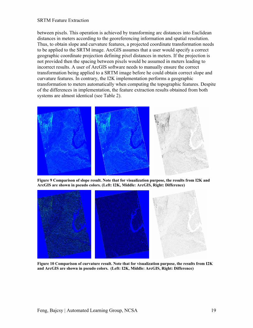
10.1 Slope Because the unit for spacing between cells in the original SRTM image is specified as Latitude/Longitude, a projected coordinate transformation needs to be applied to the image before computing the slope. Otherwise, the resulting image from ArcGIS would not be correct. The detailed is discussed in Section 10.8. After applying adequate transformation, the results from I2K and ArcGIS are almost identical (see Figure 9). 10.2 Curvature For the same reason in computing slope, an adequate transformation needs to be applied before computing the curvature. The resulting images are also quite similar after transformation (see Figure 10). 10.3 Aspect As could be observed in the test image (see Figure 11), the results from both I2K and ArcGIS are quite similar. The subtle difference in the average difference is mainly due to the fact that the aspect is a property derived from slope (which is the direction of maximum down slope), and thus it inherited the small differences when computing the slope. 10.4 Depression Filling Although we do not have the detailed definition about how ArcGIS implements depression filling, the result I2K generated is almost identical to that of ArcGIS. Note some unnatural bright spot in the ArcGIS result, which is because ArcGIS simply sets the undefined data pixel to the largest possible height value, while I2K sets them to the lowest height value in the DEM image. 10.5 Flow Direction The flow direction is encoded as the power of 2 with range from 1~128. Though there is a notable difference in the resulting image, the flow pattern is in general quite similar (see Figure 13). This difference is mainly because in I2K implementation, we use a BFS (Breadth-First Search) based criteria in determining the flow direction on flat region, while ArcGIS might use their privately developed algorithm for solving the same problem. 10.6 Flow Accumulation As a derived result of the flow direction, the flow accumulation in I2K implementation is also quite similar to that of ArcGIS. Most of the differences in flow direction take place in flat region, which usually has a large amount of flow accumulation. Thus the resulting flow accumulation difference is quite noticeable. However, the flow pattern in the resulting images looks quite similar (see Figure 14). Table 2 Average Difference for each feature between I2K and ArcGIS

Average Difference

Variable Range Unit Percentage

Slope 0.2345302 0 ~ 90 Degree 0.260 %



Curvature 0.021202 -4 ~ +4 1/100 (Meter)

0.265 %

Aspect 0.22 0 ~ 360 Degree 0.061 %

Depression Filling 2.73 -10000~10000 Meter 0.027 %

Flow Direction 6.60 1~128 5.156 %

Flow Accum. 561.23 0 ~ Max. Watershed size (668360 pixels here)

0.084 %

10.7 Statistical Robustness of Derived Features While computing slope and curvature, the partial 1st and 2nd derivatives are necessary. These derivatives are approximated using discrete difference of neighboring pixels since the input image is digital. The conventional way of finding the derivative values in an image is to use a 3x3 neighboring mask and apply finite difference method to compute the derivatives. In our I2K implementation, we also experiment with different sizes of masks to increase the statistical robustness of the result. Here we uses a 3x3 mask to mimic the ArcGIS result, a 5x5 and a 7x7 mask to experiment the better robustness due to larger neighboring mask. We apply these masks of different sizes on a 100x100 Gaussian noise white image, with mean 0.0 and standard deviation 0.5. The theoretical slope and curvature features are equal to zero across the image based on our synthetic test image preparation. The resulting differences between the theoretical and estimated feature values are summarized in Table 3. By considering the ArcGIS standard mask to be 3x3, we computed a percentage of feature estimate improvement due to a larger mask than 3x3. The percentage is presented in Table 3 inside of parentheses. The percentage numbers demonstrate the estimated improvement as the larger neighboring mask is applied. On the other side, for mountainous regions sampled at coarse spatial resolution, smaller mask size might be more appropriate. Thus, the flexibility of user-driven or data-driven mask size selection is desirable as implemented in I2K software. Table 3 Average difference between theoretical result and actual result using mask of different sizes

3x3 5x5 7x7 9x9

Slope 14.911 8.354 (43.9%) 5.766 (61.3%) 4.452 (70.1%)

Curvature 0.198 0.142 (28.3%) 0.117 (40.9%) 0.101 (49.0%)

10.8 Discussion of the Comparative Results

As part of our development, we have also encountered the problem of geographic coordinate system when comparing our results with those from ArcGIS. Reviewing the formulation of slope and curvature, we could see that the spacing between 2 pixels is needed during computation. The SRTM header does not explicitly provide this information. An adequate geographic coordinate system is needed to compute the spacing



between pixels. This operation is achieved by transforming arc distances into Euclidean distances in meters according to the georeferencing information and spatial resolution. Thus, to obtain slope and curvature features, a projected coordinate transformation needs to be applied to the SRTM image. ArcGIS assumes that a user would specify a correct geographic coordinate projection defining pixel distances in meters. If the projection is not provided then the spacing between pixels would be assumed in meters leading to incorrect results. A user of ArcGIS software needs to manually ensure the correct transformation being applied to a SRTM image before he could obtain correct slope and curvature features. In contrary, the I2K implementation performs a geographic transformation to meters automatically when computing the topographic features. Despite of the differences in implementation, the feature extraction results obtained from both systems are almost identical (see Table 2).

Figure 9 Comparison of slope result. Note that for visualization purpose, the results from I2K and ArcGIS are shown in pseudo colors. (Left: I2K, Middle: ArcGIS, Right: Difference)

Figure 10 Comparison of curvature result. Note that for visualization purpose, the results from I2K and ArcGIS are shown in pseudo colors. (Left: I2K, Middle: ArcGIS, Right: Difference)



Figure 11 Comparison of aspect result (Left: I2K, Middle: ArcGIS, Right: Difference)

Figure 12 Comparison of depression filling result (Left: I2K, Middle: ArcGIS, Right: Difference)

Figure 13 Comparison of flow direction result (Left: I2K, Middle: ArcGIS, Right: Difference)



Figure 14 Comparison of flow accumulation result (Left: I2K, Middle: ArcGIS, Right: Difference)

11 Discussion

In conclusion, we implemented the extraction of topographic features from SRTM data. We compare our results with commercial GIS package ArcGIS. The customized implementation of the feature extraction in I2K enables us to experiment new methods and ideas in computing useful features. The advantages of our implementation over ArcGIS’s include (1) providing features not supported by ArcGIS (see Table 4 for comparison), (2) improving the statistical robustness of slope and curvature (see Table 3), (3) using application customized algorithms or feature definitions, and (4) sharing our code with other researchers.

Table 4: Comparison of supported features in I2K and ArcGIS

I2K ArcGIS Comments

Slope Yes Yes

Curvature Yes Yes

Aspect Yes Yes

Depression-Free DEM Yes Yes

Sink Detection Yes No

Depression Filling

Watershed Yes No

Can’t be obtained directly in ArcGIS

Flow Direction Yes Yes

Flow Accumulation Yes Yes

Compound Topographic Index (CTI) Yes No Unsupported Ops.

Curvature Angle Yes No Unsupported Ops.



References: [Greenlee 87] Greenlee, D. D., 1987. Raster and vector processing for scanned lineword: Photogrammetric Engineering and Remote Sensing, Vol. 53, No. 10, pp. [Jenson 88] S.K. Jenson and J. O. Domingue, Extracting Topographic Structure from Digital Elevation Data for Geographic Information, PHOTOGRAMMETRIC ENGINEERING AND REMOTE SENSING, Vol. 54, No. 11, November 1988, pp. 1593-1600. [Lars 2002] Lars Arge, Jefferey S. Chase, et al. Efficient Flow Computation on Massive Grid Terrain Datasets. Department of Computer Science, Duke University. [Moore 91] Moore, I. D., Grayson, R. B., and Landson, A. R., 1991. 'Digital Terrain Modelling: a Review of Hydrological, Geomorphological, and Biological Applications' , Hydrological Processes. Vol. 5.3-30. [Zeverbergen 87] Zeverbergen, L. W., and C. R. Thorne, 1987. 'Quantitative Analysis of Land Surface Topography', Earth Surface Processes and Landforms, Vol. 12, pp 47 -56.

extracting topographic features from shuttle...

Documents