Extrasolar planets

Detections using the transit method

Schweighart Maria

Submitted to the

Institute of Physics

Geophysics, Astrophysics and Meteorology (IGAM)

in Fulfilment of the Requirements for the Degree

Bachelor of Science

at the

University of Graz, Austria

Matriculation number: 1311711

Supervisor: Ratzka Thorsten, Dipl.-Phys. Dr.rer.nat.

Graz, October 2016

3

ABSTRACT

An extrasolar planet is a planet orbiting a star other than the Sun. In the last 25 years, the

search for exoplanets got the most rapidly developing field of astrophysics. More than

3300 of these worlds are currently known and the number increases steadily. Exoplane-

tary systems share similarities with the Solar system but also show new astonishing fea-

tures like the hot Jupiters. These exoplanets are Jupiter-like but orbit in extreme proximity

to their host star. Earth-based and space missions like Kepler, COROT, and WASP were

initiated in order to detect more and more objects. The radial velocity method and the

observation of a transit event are the most successful techniques to survey exoplanets.

The observatory Lustbühel in Graz is well equipped to study transits, the passage of an

extrasolar planet in front of the star’s surface as seen from Earth. Five observations of

such events were performed and four of them were successful. A significantly visible dip

is detected in each of the measured light curves.

5

Author’s preface and acknowledgment

As far back as ancient Greece, people have wondered about the existence of other worlds

besides our Solar system in the universe. The idea of life elsewhere than our beloved

home, the Earth, is deeply entrenched in the minds of men of letters. Around 300 BC, the

Greek philosopher Epicurus stated: “There are infinite worlds both like and unlike this

world of ours. […] We must believe that in all worlds there are living creatures and plants

and other things we see in this world.” (Epicurus, 341–270 BC)

Furthermore, some believers of this concept such as the medieval scholar Giordano Bruno

(1548-1600) talked about the endlessness of the universe in the 16th century: “There are

countless suns and countless Earths all rotating around their suns in exactly the same way

as the seven planets of our system. We see only the suns because they are the largest

bodies and are luminous, but their planets remain invisible to us because they are smaller

and non-luminous. The countless worlds in the universe are no worse and no less inhab-

ited than our Earth.” (Piper, 2014, p. 4)

Ever since the idea of life elsewhere was born, the seed grew into an irresistible urge to

improve the sensitivity of instruments and advance methods of detection and observation

to search for extrasolar planets.

In my view all of the writers above once laid down to look up to the night sky, let the

thoughts wander, and took a deep breath. In these situations, while seeing the twinkling

stars and philosophizing about my life and problems, I sometimes wonder if there is some-

one else looking my way, watching our Sun. This special thrill drove me to stick my nose

into astronomical books and papers about the latest achievements in this field of extraso-

lar planets.

The main goal of this bachelor thesis is to give a general insight of the various techniques

to detect an extrasolar object and to determine the properties of the observed exoplanets.

Fortunately, my supervisor Ratzka Thorsten provided access to the observatory Graz-

Lustbühel where I was able to study five different transits of extrasolar planets. The avail-

able equipment allowed to track the star and to measure the flux variation. Appropriate

computer programs to analyse the amount of received data were installed by the observa-

tory as well.

At this point I would like to thank those people who helped me write this thesis. First of

all, many thanks to my beloved family, my parents who raised me in a way that made me

this open-minded and curious person I am today, and my siblings, Angelika and Thomas,

6

for their generous support in every aspect of life. I am so grateful for all the people who

accompanied my way and motivated me to follow my dreams. I really do not know how

to thank my supervisor Dr. Ratzka for giving me this huge opportunity to slip into the

role of the scientist and helping me to sort the massive amount of data.

7

CONTENT

ABSTRACT ..................................................................................................................... 3

AUTHOR’S PREFACE AND ACKNOWLEDGMENT ............................................. 5

LIST OF FIGURES ........................................................................................................ 9

LIST OF TABLES ........................................................................................................ 11

LIST OF ABBREVIATIONS AND SYMBOLS ........................................................ 13

1 INTRODUCTION ............................................................................................. 15

1.1 What is an extrasolar planet? .......................................................................... 15

1.2 The way to success............................................................................................. 15

1.3 How many are there? ........................................................................................ 16

1.4 Observatories for exoplanet transits ............................................................... 17

1.5 How to name them all ....................................................................................... 18

1.6 Exoplanet types ................................................................................................. 19

1.6.1 Terrestrial planets ................................................................................................ 19

1.6.2 Gas giants ............................................................................................................ 19

1.6.3 Eccentrics ............................................................................................................ 21

1.6.4 Free-floaters ........................................................................................................ 21

1.7 Comparison to the Solar system ...................................................................... 21

2 DETECTION METHODS ............................................................................... 23

2.1 Radial velocity measurements.......................................................................... 23

2.2 Astrometry ......................................................................................................... 25

2.3 Transit method .................................................................................................. 26

2.4 Gravitational lensing......................................................................................... 29

2.5 Pulsar timing ..................................................................................................... 30

3 OBSERVATION ............................................................................................... 31

3.1 Observatory Graz - Lustbühel ......................................................................... 31

3.1.1 Equipment ........................................................................................................... 31

3.1.2 Data analysis ....................................................................................................... 31

3.1.3 Observation routine ............................................................................................. 32

3.2 WASP-104 b....................................................................................................... 33

3.3 HAT-P-12 b ........................................................................................................ 37

3.4 EPIC-211089792 b............................................................................................. 40

3.5 XO-1 b ................................................................................................................ 42

3.6 HAT-P-5 b .......................................................................................................... 45

4 CONCLUSION.................................................................................................. 49

5 LIST OF REFERENCES ................................................................................. 51

6 APPENDIX ........................................................................................................ 53

6.1 WASP-104 b....................................................................................................... 53

8

6.2 HAT-P-12 b ........................................................................................................ 54

6.3 EPIC-211089792 b ............................................................................................. 54

6.4 XO-1 b................................................................................................................. 55

6.5 HAT-P-5 b .......................................................................................................... 56

9

List of figures

Figure 1: Evolution in number of discoveries. (NASA Exoplanet Archive, 2016) ........ 16

Figure 2: Jupiter-mass objects in proximity to host star. (NASA Exoplanet Archive, 2016)

........................................................................................................................................ 20

Figure 3: Jupiter-like planets. (NASA Exoplanet Archive, 2016) .................................. 22

Figure 4: eccentricity. (NASA Exoplanet Archive, 2016) .............................................. 22

Figure 5: Orbital motion of 51 Peg. (Mayor & Queloz, 1995, p. 357) ........................... 25

Figure 6: Schematic light curve of a transit event. (Adapted from Deeg, 2002) ............ 26

Figure 7: Impact parameter (Adapted from Cowley & Hughes, 2014, following Haswell,

2010). .............................................................................................................................. 27

Figure 8: Transit length (Adapted from Cowley & Hughes, 2014, following Haswell,

2010). .............................................................................................................................. 28

Figure 9: Geometry referring to transit duration (Adapted from Cowley & Hughes, 2014,

following Haswell, 2010). .............................................................................................. 28

Figure 10: Light curve of a microlensing event OGLE-2005-BLG-390. (Beaulieu, J.-P. et

al., 2006) ......................................................................................................................... 29

Figure 11: WASP-104 b / position of science target and calibrator ............................... 34

Figure 12: WASP-104 b: flux ratio during transit event ................................................ 34

Figure 13: HAT-P-12 b / position of science target and calibrators ............................... 37

Figure 14: HAT-P-12 b: flux ratio during transit event .................................................. 38

Figure 15: EPIC-211089792 b / position of science target and calibrators .................... 41

Figure 16: XO-1 b / position of science target and calibrator ........................................ 42

Figure 17: XO-1 b: flux ratio during transit event .......................................................... 43

Figure 18: HAT-P-5 b / position of science target and calibrators ................................. 45

Figure 19: HAT-P-5 b: flux ratio during transit event .................................................... 46

Figure 20: WASP-104 b: Relative flux in area and aperture .......................................... 53

Figure 21: HAT-P-12 b: Relative flux in area and aperture ........................................... 54

Figure 22: EPIC-211089792 b: Relative flux in area and aperture ................................ 54

Figure 23: EPIC-211089792 b: flux ratio of star and calibrators during transit event ... 55

Figure 24: XO-1 b: Relative flux in area and aperture ................................................... 55

Figure 25: HAT-P-5 b: Relative flux in area and aperture ............................................. 56

11

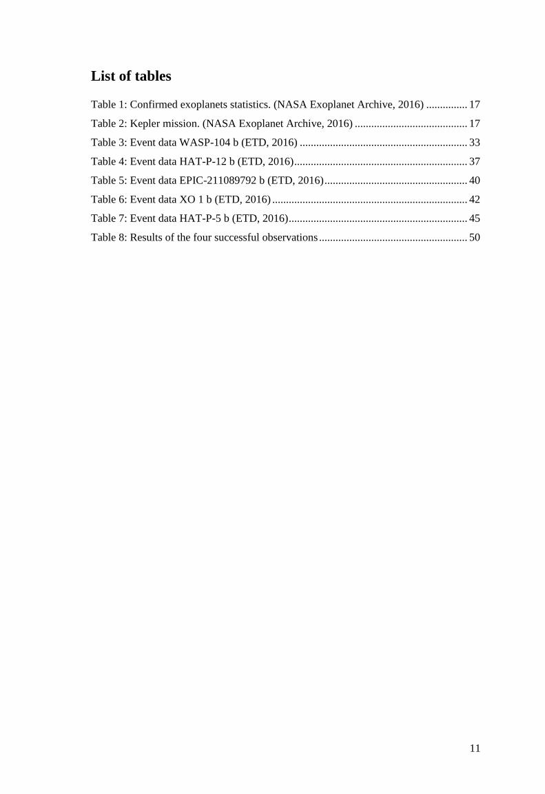
List of tables

Table 1: Confirmed exoplanets statistics. (NASA Exoplanet Archive, 2016) ............... 17

Table 2: Kepler mission. (NASA Exoplanet Archive, 2016) ......................................... 17

Table 3: Event data WASP-104 b (ETD, 2016) ............................................................. 33

Table 4: Event data HAT-P-12 b (ETD, 2016) ............................................................... 37

Table 5: Event data EPIC-211089792 b (ETD, 2016) .................................................... 40

Table 6: Event data XO 1 b (ETD, 2016) ....................................................................... 42

Table 7: Event data HAT-P-5 b (ETD, 2016) ................................................................. 45

Table 8: Results of the four successful observations ...................................................... 50

13

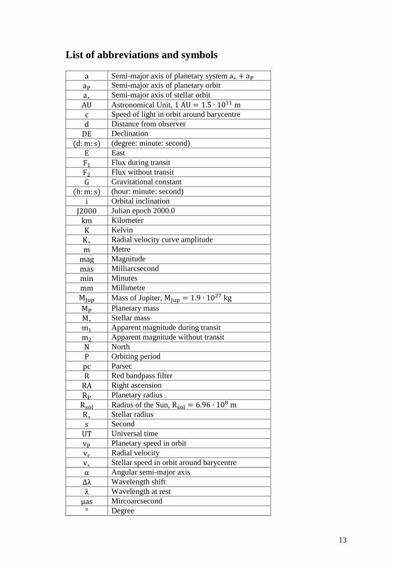
List of abbreviations and symbols

a Semi-major axis of planetary system a∗ + aP

aP Semi-major axis of planetary orbit

a∗ Semi-major axis of stellar orbit

AU Astronomical Unit, 1 AU = 1.5 ∙ 1011 m

c Speed of light in orbit around barycentre

d Distance from observer

DE Declination

(d:m: s) (degree: minute: second)

E East

F1 Flux during transit

F2 Flux without transit

G Gravitational constant

(h:m: s) (hour: minute: second)

i Orbital inclination

J2000 Julian epoch 2000.0

km Kilometer

K Kelvin

K∗ Radial velocity curve amplitude

m Metre

mag Magnitude

mas Milliarcsecond

min Minutes

mm Millimetre

MJup Mass of Jupiter, MJup = 1.9 ∙ 1027 kg

MP Planetary mass

M∗ Stellar mass

m1 Apparent magnitude during transit

m2 Apparent magnitude without transit

N North

P Orbiting period

pc Parsec

R Red bandpass filter

RA Right ascension

RP Planetary radius

Rsol Radius of the Sun, Rsol = 6.96 ∙ 108 m

R∗ Stellar radius

s Second

UT Universal time

vP Planetary speed in orbit

vr Radial velocity

v∗ Stellar speed in orbit around barycentre

α Angular semi-major axis

∆λ Wavelength shift

λ Wavelength at rest

µas Mircoarcsecond

° Degree

15

1 Introduction

1.1 What is an extrasolar planet?

With the discovery of Eris, the International Astronomical Union (IAU) was forced to

create new definitions for the planetary bodies found in the Solar system. Originally the

word “planet” described “wanderers”, moving lights in the sky. In 2006 the IAU released

the updated definition:

“A ‘planet’ is a celestial body that (1) orbits the Sun, (2) has sufficient mass for its self-

gravity to overcome rigid body forces so that it assumes a hydrostatic equilibrium (nearly

round) shape, and (3) has cleared the neighbourhood around its orbit.” (IAU, 2006)

As the name suggests an extrasolar planet or exoplanet is a planet orbiting a star other

than the Sun. Possible nomenclatures one might come across are exoplanets, extrasolar

planet, or – when the planet’s properties resemble that of a planet in the Solar system –

exo-Earth, exo-Jupiter.

1.2 The way to success

By now our Solar system is known by heart in comparison to the hidden places beyond

our “home”. So there is of course the desire to broaden our horizon to see if there is an

Earth-like planet capable of harbouring some kind of life. Many science-fiction films and

artistic interpretations put different pictures in our minds of what these worlds could look

like and no limit will restrict the individual imagination. In contrast, scientists always aim

to understand reality as accurate as possible. Hence the quest for the seemingly strange

places was and is still driving some ambitious programmes of research.

In the mid-20th century exoplanets were set in a tighter focus. The first hints of a terrestrial

object orbiting a star other than the Sun were announced at the end of the 1980s. In 1992

the existence of worlds beyond our Solar system was verified by the discovery of a plan-

etary system around the millisecond pulsar PSR B1257+12. 1995 needs to be highlighted

because the first object orbiting a solar-type main-sequence star (51 Pegasi) was measured

by the Swiss astronomers Mayor and Queloz. Approximately 15 pc from Earth the gas

giant 51 Pegasi b which is half the mass of Jupiter orbits its host star at a distance of 0.05

AU in just 4.2 days. The variation in the radial velocity revealed the planet. For years the

radial velocity method was the only one to provide reasonable results. However, this

planet does not offer the necessary surface conditions to support some form of life. Taking

the star’s properties and the separation between both objects, the surface temperature is

16

estimated to be 1250 K. That is why exoplanets like this one are called “hot Jupiters”.

(Piper, 2014, p. 24-28)

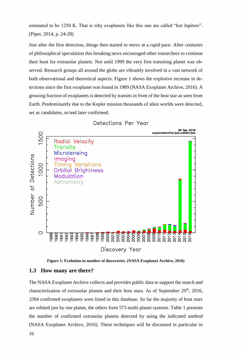
Just after the first detection, things then started to move at a rapid pace. After centuries

of philosophical speculation this breaking news encouraged other researchers to continue

their hunt for extrasolar planets. Not until 1999 the very first transiting planet was ob-

served. Research groups all around the globe are vibrantly involved in a vast network of

both observational and theoretical aspects. Figure 1 shows the explosive increase in de-

tections since the first exoplanet was found in 1989 (NASA Exoplanet Archive, 2016). A

growing fraction of exoplanets is detected by transits in front of the host star as seen from

Earth. Predominantly due to the Kepler mission thousands of alien worlds were detected,

set as candidates, or/and later confirmed.

Figure 1: Evolution in number of discoveries. (NASA Exoplanet Archive, 2016)

1.3 How many are there?

The NASA Exoplanet Archive collects and provides public data to support the search and

characterization of extrasolar planets and their host stars. As of September 29th, 2016,

3394 confirmed exoplanets were listed in this database. So far the majority of host stars

are orbited just by one planet, the others form 573 multi-planet systems. Table 1 presents

the number of confirmed extrasolar planets detected by using the indicated method

(NASA Exoplanet Archive, 2016). These techniques will be discussed in particular in

17

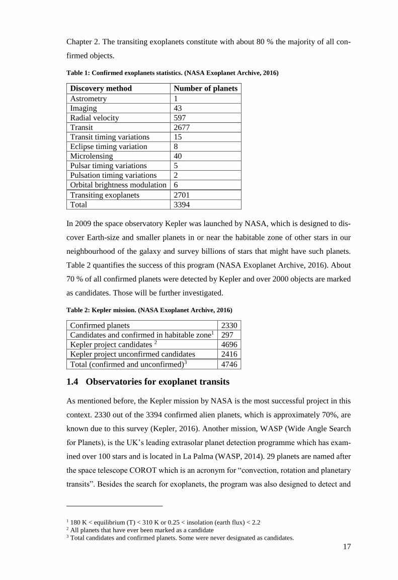
Chapter 2. The transiting exoplanets constitute with about 80 % the majority of all con-

firmed objects.

Table 1: Confirmed exoplanets statistics. (NASA Exoplanet Archive, 2016)

Discovery method Number of planets

Astrometry 1

Imaging 43

Radial velocity 597

Transit 2677

Transit timing variations 15

Eclipse timing variation 8

Microlensing 40

Pulsar timing variations 5

Pulsation timing variations 2

Orbital brightness modulation 6

Transiting exoplanets 2701

Total 3394

In 2009 the space observatory Kepler was launched by NASA, which is designed to dis-

cover Earth-size and smaller planets in or near the habitable zone of other stars in our

neighbourhood of the galaxy and survey billions of stars that might have such planets.

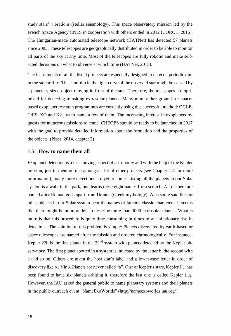
Table 2 quantifies the success of this program (NASA Exoplanet Archive, 2016). About

70 % of all confirmed planets were detected by Kepler and over 2000 objects are marked

as candidates. Those will be further investigated.

Table 2: Kepler mission. (NASA Exoplanet Archive, 2016)

Confirmed planets 2330

Candidates and confirmed in habitable zone1 297

Kepler project candidates 2 4696

Kepler project unconfirmed candidates 2416

Total (confirmed and unconfirmed)3 4746

1.4 Observatories for exoplanet transits

As mentioned before, the Kepler mission by NASA is the most successful project in this

context. 2330 out of the 3394 confirmed alien planets, which is approximately 70%, are

known due to this survey (Kepler, 2016). Another mission, WASP (Wide Angle Search

for Planets), is the UK’s leading extrasolar planet detection programme which has exam-

ined over 100 stars and is located in La Palma (WASP, 2014). 29 planets are named after

the space telescope COROT which is an acronym for “convection, rotation and planetary

transits”. Besides the search for exoplanets, the program was also designed to detect and

1 180 K < equilibrium (T) < 310 K or 0.25 < insolation (earth flux) < 2.2 2 All planets that have ever been marked as a candidate 3 Total candidates and confirmed planets. Some were never designated as candidates.

18

study stars’ vibrations (stellar seismology). This space observatory mission led by the

French Space Agency CNES in cooperation with others ended in 2012 (COROT, 2016).

The Hungarian-made automated telescope network (HATNet) has detected 57 planets

since 2003. These telescopes are geographically distributed in order to be able to monitor

all parts of the sky at any time. Most of the telescopes are fully robotic and make self-

acted decisions on what to obverse at which time (HATNet, 2015).

The instruments of all the listed projects are especially designed to detect a periodic dim

in the stellar flux. The short dip in the light curve of the observed star might be caused by

a planetary-sized object moving in front of the star. Therefore, the telescopes are opti-

mized for detecting transiting extrasolar planets. Many more either ground- or space-

based exoplanet research programmes are currently using this successful method: OGLE,

TrES, XO and K2 just to name a few of them. The increasing interest in exoplanets re-

quests for numerous missions to come. CHEOPS should be ready to be launched in 2017

with the goal to provide detailed information about the formation and the properties of

the objects. (Piper, 2014, chapter 2)

1.5 How to name them all

Exoplanet detection is a fast-moving aspect of astronomy and with the help of the Kepler

mission, just to mention one amongst a lot of other projects (see Chapter 1.4 for more

information), many more detections are yet to come. Listing all the planets in our Solar

system is a walk in the park, one learns these eight names from scratch. All of them are

named after Roman gods apart from Uranus (Greek mythology). Also some satellites or

other objects in our Solar system bear the names of famous classic characters. It seems

like there might be no more left to describe more than 3000 extrasolar planets. What is

more is that this procedure is quite time consuming in times of an inflationary rise in

detections. The solution to this problem is simple: Planets discovered by earth-based or

space telescopes are named after the mission and ordered chronologically. For instance,

Kepler 22b is the first planet in the 22nd system with planets detected by the Kepler ob-

servatory. The first planet spotted in a system is indicated by the letter b, the second with

c and so on. Others are given the host star’s label and a lower-case letter in order of

discovery like 61 Vir b. Planets are never called “a”. One of Kepler's stars, Kepler 11, has

been found to have six planets orbiting it, therefore the last one is called Kepler 11g.

However, the IAU asked the general public to name planetary systems and their planets

in the public outreach event “NameExoWorlds” (http://nameexoworlds.iau.org/).

19

1.6 Exoplanet types

The found extrasolar planets are classified according to the categories below. Of course

subdivisions or intermediary groups are created to describe the object in greater detail but

for now the listed types are sufficient to get a satisfactory idea of the planets´ properties.

(Piper, S., 2014, p. 81-89, adapted from Lammer, H. et al., 2009)

1.6.1 Terrestrial planets

Features like mass, radius, and atmosphere are similar to those of the Earth. These “exo-

Earths” are located in the habitable zone of the parent star allowing water to appear in its

liquid form. For scientists these ones are like the holy grail because their conditions are

most likely to support life. The detection of those rocky planets is, however, difficult for

the transit method due to the fact that exo-Earths are quite small, approximately 10000

km in diameter. Their low mass causes also no large radial velocity modulation. That is

why only a few have been found yet.

The term “super” in “Super Earths” merely indicates the planet’s mass which can go up

to 10 times the mass of our Earth. Despite this fact they show a rocky surface and an

atmosphere that could be analysed by spectral methods during a transit. For these small

planets it is even hard to tell if there is an atmosphere or not.

Entirely water covered planets are called water worlds. Not yet discovered, these exoplan-

ets are believed to have been built out of ice and rocks in the outer zone of the young

planetary system. During their inward migration they heat up and the ice melts.

1.6.2 Gas giants

Examples of this exoplanet type are even found in our Solar system: Jupiter and Saturn.

Neptune and Uranus are obviously counted as gas giants but sometimes referred to as ice

giants because they contain larger fractions of heavier materials like methane and ammo-

niac. If Jupiter had collected 80 times more material during its formation process in the

protostellar cloud, it would have become a star. The process of nuclear fusion of hydrogen

is required for this title. A gas planet’s mass is mostly composed of hydrogen and helium

with potentially a dense rocky or metallic core. The mass’ minimum for gas giants is set

to be 10 times the Earth’s mass.

Planets that are similar in mass to Jupiter and are orbiting the parent star in direct prox-

imity within a few days are called hot Jupiters. The term “hot” referrers to surface tem-

peratures significantly higher than the one on Jupiter. Furthermore, the short distance

causes a tidal locking which means that one side of a planet always faces the star. This

effect is also known as synchronous rotation or captured rotation. Hot Jupiters show orbits

20

with a low eccentricity and are easy to detect with the radial velocity and the transit

method. That is why most of the discovered planets are members of this category. As well

as objects of other types, hot Jupiters are believed to have migrated towards the central

star after their formation.

Very hot Jupiters have to deal with even more extreme circumstances than hot Jupiters.

They orbit much closer than Mercury around our Sun. The object OGLE-TR-56 which is

about the mass of Jupiter orbits its host star in 1.2 days at a distance of 6000 km. Addi-

tionally, the extreme proximity causes even higher temperatures giving the planets a good

“roast”. These planets have to be formed in the outer zone of the system because so close

to the star, there could not have been enough material. Numerous theories try to explain

this migration phenomenon and the involved forces but that represents a whole new issue

in the exoplanet research which will not be covered in this thesis.

Figure 2 significantly shows concentrations of Jupiter-mass objects orbiting the parent

star with semi-major axes around and even below 0.1 AU (NASA Exoplanet Archive,

2016).

Figure 2: Jupiter-mass objects in proximity to host star. (NASA Exoplanet Archive, 2016)

Planets of this category “hot Neptune” are similar in mass and density to Neptune or

Uranus but have orbits with radii of less than 1 AU. That is why they show a warmer

atmosphere. Again, they should have been formed in the outer disk and then migrated

inwards.

So-called Chthonian planets were originally gas giants like hot Jupiters. They moved far

too close to the central star and their H/He envelope was stripped away, leaving only the

rocky or metallic cores. The remnants resemble terrestrial planets.

21

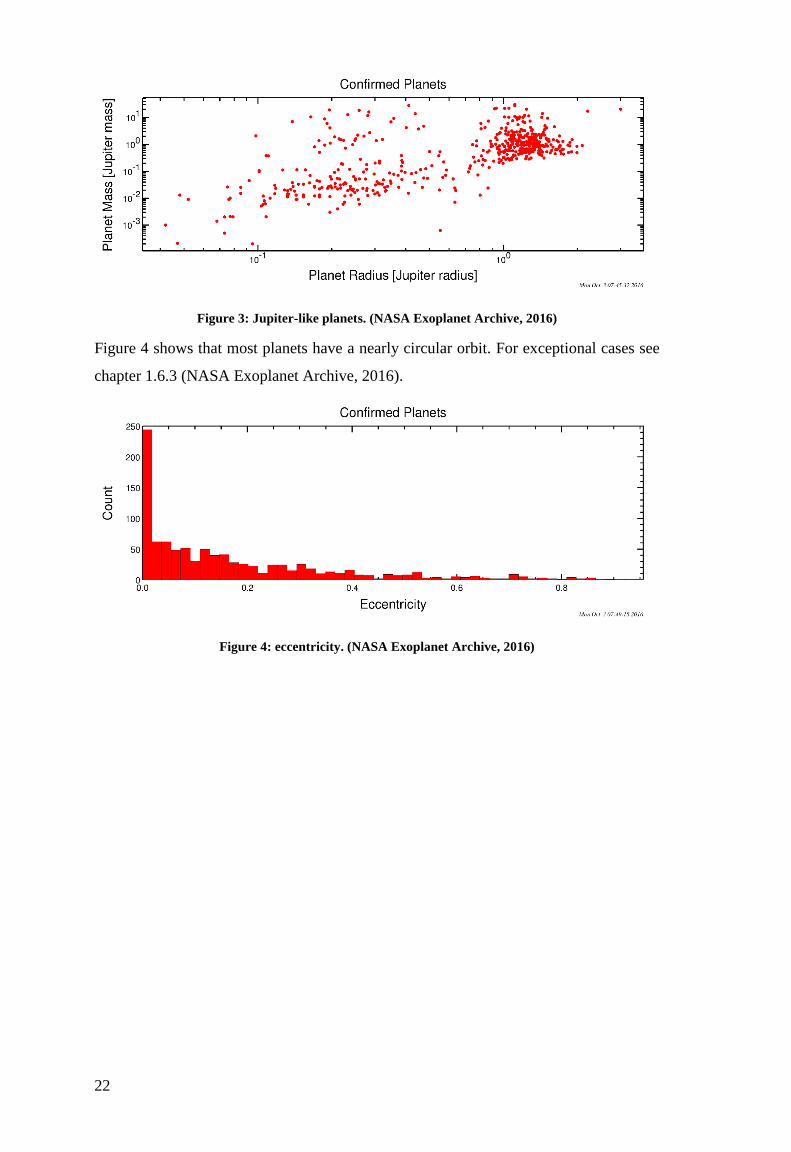
1.6.3 Eccentrics

Great eccentricity of the orbit is the main property of these extrasolar planets. As a result,

the surface temperature varies dramatically during an orbit. The objects HD 20782 b and

HD 80606 b even show an eccentricity of e = 0.97, 0.93, respectively.

1.6.4 Free-floaters

These orphan planets are quite intriguing due to the fact that they do not orbit a star.

Rogue planets, as they are referred to as well, are free-floating in the galaxy. It is believed

that they either have somehow been ejected from the developing star system or have

formed early in the Universe and have never been bound to a star (ESO 1245, 2012).

1.7 Comparison to the Solar system

Some features of the exoplanetary systems are shared with our home system. Most of the

stars hosting planets are main-sequence stars similar to the Sun because solar-type stars

are primarily observed. The majority of the confirmed extrasolar planets are the Jovian

planets. Only a limited number of terrestrial planets has been found yet. A reason for that

is the fact that detection methods are designed to look for massive bodies orbiting close

to the host star. About 360 planets possess a radius smaller than 1.25 Earth radius and 28

resemble the Earth in mass (NASA Exoplanet Archive, 2016).

Most exoplanets are gaseous similar to gas giants made of hydrogen and helium gas. Oth-

ers show a rockier, Earth-like composition. The so-called hot Jupiters are similar in mass

to Jupiter and some orbit their parent star even closer than Mercury orbits the Sun. Theory

does not allow massive objects to form in proximity to the central star. That is why it is

believed that those hot Jupiters have been formed in an outer zone of the system and

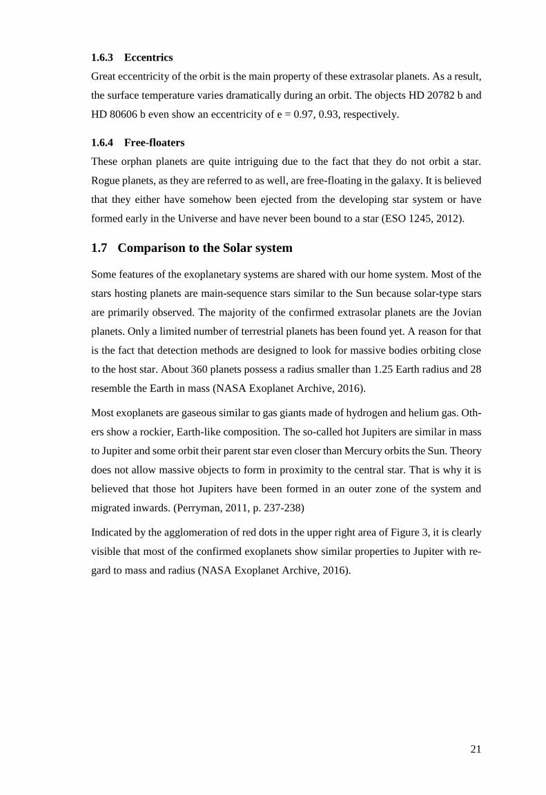
migrated inwards. (Perryman, 2011, p. 237-238)

Indicated by the agglomeration of red dots in the upper right area of Figure 3, it is clearly

visible that most of the confirmed exoplanets show similar properties to Jupiter with re-

gard to mass and radius (NASA Exoplanet Archive, 2016).

22

Figure 3: Jupiter-like planets. (NASA Exoplanet Archive, 2016)

Figure 4 shows that most planets have a nearly circular orbit. For exceptional cases see

chapter 1.6.3 (NASA Exoplanet Archive, 2016).

Figure 4: eccentricity. (NASA Exoplanet Archive, 2016)

23

2 Detection methods

In order to discover and observe an extrasolar planet, more precise and powerful instru-

ments and sophisticated techniques need to be used. It was not until NASA’s mission

New Horizons in 2015 that a high quality picture of the dwarf planet Pluto at the outer

edge of our own Sol system was taken. How can it be possible to detect an exoplanet

much further away from Earth? The Earth’s atmosphere limits the accuracy of the obser-

vations in addition. To eliminate diffraction and scattering in the atmosphere space ob-

servatories were installed. The methods to overcome the difficulties of detecting extraso-

lar planets are divided in direct and indirect techniques.

Taking actual images of the planet (all planets outside the Solar system stay unresolved,

anyway) or extracting the planet’s electromagnetic spectrum, which tells scientists about

the atmospheric composition, falls under the category of direct methods. Directly observ-

ing exoplanets is very challenging, not only because of the interstellar distance but also

because the star’s brightness blinds the instrument used to detect the much fainter planet.

The investigation is made even more difficult by the fact that the angular separation be-

tween the planet and its host star is generally small.

The three most commonly used methods (radial velocity, astrometry, transit) are referred

to as indirect. Instead of detecting the planet itself its effects on the host star are recorded

as a proof for the planet’s existence. Both planet and star orbit around the common centre

of mass. On the one hand the central star’s motion can be influenced by the planet (radial

velocity, astrometric method), on the other hand the star’s light can be slightly dimmed

by a transiting object (transit method). Gravitational lensing and pulsar timing are also

indirect detection methods. (Mason, 2008, p. 2)

2.1 Radial velocity measurements

In the Solar system it seems like the Sun represents the centre of mass because it is enor-

mously massive compared to the planets. In reality all bodies orbit a common centre of

mass located inside the Sun’s surface. Due to the gravitational pull of the planet(s) stars

wobble around this barycentre causing the light spectrum to shift. The radial velocity

method records these periodic Doppler shifts in the stellar spectrum in order to examine

the properties of the exoplanetary system. If the star moves toward the observer on Earth,

the light emitted has a shorter wavelength and the absorption lines are blue shifted (neg-

ative radial velocity). A red shift occurs when the star is drifting away from Earth causing

a longer wavelength (positive radial velocity). There will be no shift if the star is moving

24

perpendicular to the line of sight. Just a periodic shift in frequency indicates the presence

of one or even more planets. For ground-based observatories the limiting value for this

Doppler shift is about 1 m/s.

This procedure is most efficient for massive planets in proximity to smaller host stars

because of the stronger gravitational pull of the planets (cf. hot Jupiter). Both the star and

the planet orbit the centre of mass which includes that the objects’ centre must be on

different sides of the barycentre at any time. This results in the fact that the star orbits in

the same time as the planet does. Concluding, the period of the planet is obtained by

determining the period of the radial velocity curve of the star. Furthermore, if the mass of

the planet increases, the radius of the star’s orbit around the barycentre gets larger. As it

still takes the same amount of time to complete an orbit the star has to move faster which

is indicated by a higher amplitude of the radial velocity curve.

Relevant equations to describe this method are given below (Waldmann, 2014). The

definition of all used parameters can be found in the list of abbreviations and symbols on

page 13. By determining the shift in wavelenght compared to the wavelength at rest, the

radial velocity is obtained as follows:

∆𝜆

𝜆=𝑣𝑟𝑐

( 1 )

For the system planet – star the conservation of momentum applies:

𝑀∗𝑣∗ = 𝑀𝑃𝑣𝑃 ( 2 )

Kepler’s third law sets the semi-major axes in relation to the bodies’ mass:

𝑎3 =𝐺(𝑀∗ +𝑀𝑃)

4𝜋2𝑃2

( 3 )

𝑎∗ =𝑀𝑃

𝑀∗ +𝑀𝑃𝑎 ( 4 )

The stellar speed due to the gravitational pull of the planet is calculated with the following

formula:

𝑣∗ =2𝜋𝑎∗𝑃

(4)→ 𝑣∗ ≃

2𝜋𝑎𝑀𝑃𝑃𝑀∗

( 5 )

This leads to a radial velocity curve amplitude 𝐾∗ ≃ 𝑣∗ 𝑠𝑖𝑛(𝑖).

In the early days of extrasolar planet research the radial velocity method was responsible

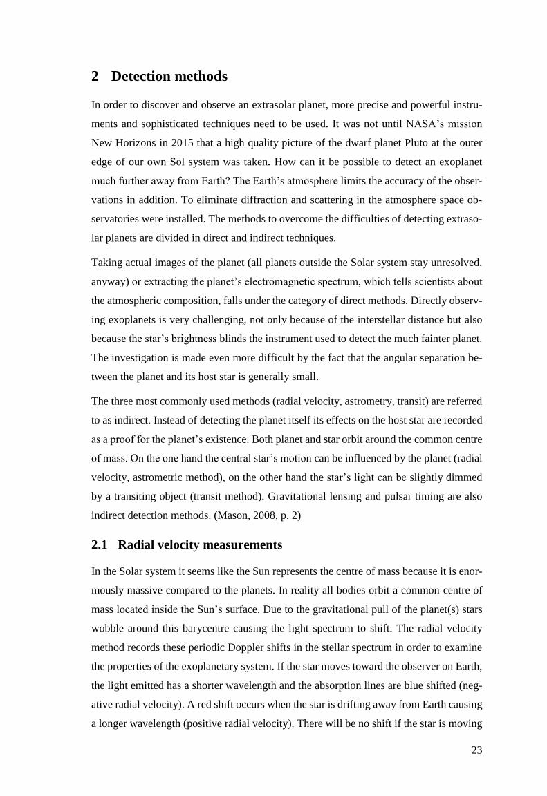
for the majority of the discovered bodies. The first “Jupiter-mass companion to a solar-

type star”, as their article is called, was detected by Mayor and Queloz in 1995 using this

25

technique. Figure 5 shows the obtained radial velocity curve of 51 Peg (Mayor & Queloz,

1995, p. 357). As of mid-2016, nearly 600 planets are identified that way (NASA Ex-

oplanet Achieve).

Figure 5: Orbital motion of 51 Peg. (Mayor & Queloz, 1995, p. 357)

2.2 Astrometry

The astrometric method is designed to record the transverse component of the periodic

motion of the parent star around the barycentre induced by the gravitational pull of the

orbiting planet. In contrast, the radial velocity technique measures the displacement along

the line of sight. A series of high accuracy observations of the angular position of the star

is needed to obtain an evidence of the existence of an exoplanet. Until now only one

planet was detected and confirmed. But this planet was already known by other detection

methods. The wobbles are simply too small to be routinely recorded by the current optical

systems.

The motion of the star orbiting the barycentre projected on the plane of the sky appears

as an ellipse with angular semi-major axis α:

𝛼 =𝑀𝑃

𝑀∗ +𝑀𝑃𝑎 ≃

𝑀𝑃𝑀∗𝑎 ≡ (

𝑀𝑃𝑀∗) (

𝑎

1 𝐴𝑈) (

𝑑

1𝑝𝑐)−1

𝑎𝑟𝑐𝑠𝑒𝑐 ( 6 )

The planet’s mass can be neglected because of the small contribution compared to the

star’s mass. The farther the exoplanetary system is located away from to the observer, the

higher is the minimal detectable planetary mass. Astrometry is most effective for a mas-

sive planet orbiting at a large separation from the star because this leads to large semi-

26

major axes of the apparent motion of the star. The method thus favours long orbital peri-

ods. But long orbits require long-term monitoring. (Perryman, 2011, p. 62-63)

ESA’s space astrometry mission Hipparcos achieved an accuracy of about 1 mas while

its operation till 1993. Currently, the best precision of about 20 µas is provided by ESA’s

mission Gaia which is a wide-angle survey observing about a billion stars in our galaxy.

The Keck telescope as a ground-based observatory also offers accuracy at this scale. The

discovery of an Earth-mass planet at a distance of 10 pc orbiting a Sun-like star at 1 AU

requires submicroarcsecond precision. By now only one confirmed planet has been found

by astrometry.

2.3 Transit method

Transit events are well known from our own Solar system (Venus, Mercury). This indirect

observational technique detects the periodic dimming of the star’s brightness due to an

exoplanet transiting in front of the star’s disk as seen from Earth. This temporary decrease

of the starlight’s intensity provides information about the extrasolar planet’s and the host

star’s properties. The dip in intensity is of the order of 1 %. What is absolutely necessary

for the application of this method is an orbital inclination close to 90 °.

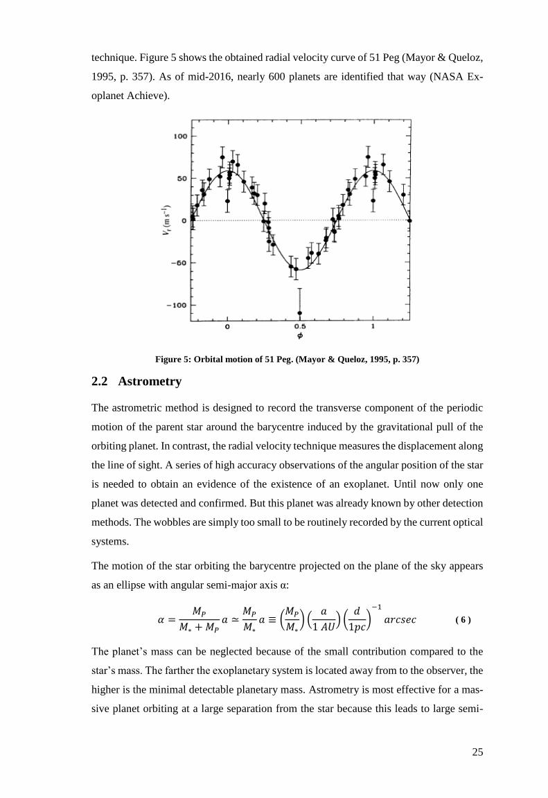
Figure 6 shows the schematic transit of a planet. The corresponding light curve is indi-

cated by the red line (Adapted from Deeg, 2002).

Figure 6: Schematic light curve of a transit event. (Adapted from Deeg, 2002)

The orbiting period is determined by the time span between two transit events. Kepler’s

third law relates the period P to the semi-major axis of the orbit a and the total mass of

the objects (𝑀𝑃 +𝑀∗):

27

𝑎3

𝑃2=𝐺(𝑀∗ +𝑀𝑃)

4𝜋2 ( 7 )

As mentioned above the transit light curve acts instructively with respect to the charac-

terization of the planet. The change in flux ΔF relative to the stellar flux F prior to the

transit can be written as:

∆F

F=RP2

R∗2 ( 8 )

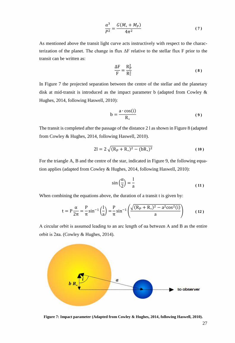
In Figure 7 the projected separation between the centre of the stellar and the planetary

disk at mid-transit is introduced as the impact parameter b (adapted from Cowley &

Hughes, 2014, following Haswell, 2010):

b =a ∙ cos(i)

R∗ ( 9 )

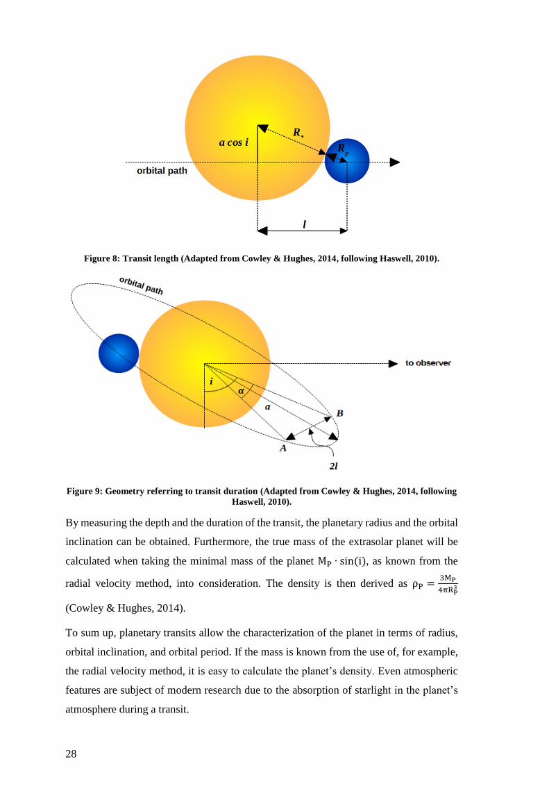
The transit is completed after the passage of the distance 2 l as shown in Figure 8 (adapted

from Cowley & Hughes, 2014, following Haswell, 2010).

2l = 2 √(RP + R∗)2 − (bR∗)2 ( 10 )

For the triangle A, B and the centre of the star, indicated in Figure 9, the following equa-

tion applies (adapted from Cowley & Hughes, 2014, following Haswell, 2010):

sin (α

2) =

l

a

( 11 )

When combining the equations above, the duration of a transit t is given by:

t = Pα

2π=P

πsin−1 (

l

a) =

P

πsin−1 (

√(RP + R∗)2 − a2cos2(i)

a) ( 12 )

A circular orbit is assumed leading to an arc length of αa between A and B as the entire

orbit is 2πa. (Cowley & Hughes, 2014).

Figure 7: Impact parameter (Adapted from Cowley & Hughes, 2014, following Haswell, 2010).

28

Figure 8: Transit length (Adapted from Cowley & Hughes, 2014, following Haswell, 2010).

Figure 9: Geometry referring to transit duration (Adapted from Cowley & Hughes, 2014, following

Haswell, 2010).

By measuring the depth and the duration of the transit, the planetary radius and the orbital

inclination can be obtained. Furthermore, the true mass of the extrasolar planet will be

calculated when taking the minimal mass of the planet MP ∙ sin (i), as known from the

radial velocity method, into consideration. The density is then derived as ρP =3MP

4πRP3

(Cowley & Hughes, 2014).

To sum up, planetary transits allow the characterization of the planet in terms of radius,

orbital inclination, and orbital period. If the mass is known from the use of, for example,

the radial velocity method, it is easy to calculate the planet’s density. Even atmospheric

features are subject of modern research due to the absorption of starlight in the planet’s

atmosphere during a transit.

29

The detection of transiting extrasolar planets has been a huge success since the first con-

firmed planet detected with this method in 1999. As of mid-2016 more than 2600 trans-

iting exoplanets are discovered and they represent about 80 % of all confirmed bodies.

The majority of them were found by NASA’s Kepler mission (NASA Exoplanet Ar-

chive).

2.4 Gravitational lensing

The bending of light by gravity is a fascinating aspect of general relativity. Electromag-

netic waves coming from a distant background object (source) are bent by the gravita-

tional potential of a foreground body (lens) when passing near it to reach the observer.

The image of the source is distorted and appears temporarily magnified. The brightness

of the source in- and decreases as the lensing object passes in front of the source. The

gravitational field of an accompanying planet to a passing lensing star can lead to an

additional amplification of the source images which means that star and planet act to-

gether as a multiple lens. (Perryman, 2011, p. 83-84)

The observation of a microlensing event not merely tells about the presence of a planet

and magnifies the starlight coming from a distant source, but also represents the only way

to detect free-floating objects. The method is responsible for the discovery of 40 extraso-

lar bodies (NASA Exoplanet Archive).

In Figure 10 the received light curve of a microlensing event is displayed in order to get

an impression of the additional amplification of the source image (Beaulieu, J.-P. et al.,

2006).

Figure 10: Light curve of a microlensing event OGLE-2005-BLG-390. (Beaulieu, J.-P. et al., 2006)

30

2.5 Pulsar timing

A rapidly spinning neutron star with a strong magnetic field is called a pulsar. As they

rotate and their spin axis is not identical to the orientation of the magnetic field axis,

pulsars emit intense electromagnetic pulses regularly. These extremely precise and stable

pulses are recorded on Earth. Once again the star’s motion around the barycentre of the

system caused by the presence of an extrasolar planet represents the starting point of the

timing method. If the pulsar is moving away from the observer when orbiting the centre

of mass, the time between each pulse becomes longer and vice versa the movement to-

wards the Earth results in shorter intervals. By precisely measuring the variations in pulse

timing scientists are able not only to deduce the existence of an exoplanet, but also the

orbit and the mass of the object. Pulsar timing is capable of recording Earth-mass and

even smaller bodies. (Perryman, 2011, p. 75)

In 1992 the pulsar timing method was used by Wolszczan and Frail to detect the very first

exoplanet around the millisecond pulsar PSR B1257+12. This planet shows the lowest

exoplanetary mass of just 0.02 Earth mass. (Wolszczan & Frail, 1992)

31

3 Observation

3.1 Observatory Graz - Lustbühel

Since its establishment in 1976 the observatory Lustbühel located at the eastern outskirts

of Graz has served as a venue of research in the fields of astronomy and telecommunica-

tions managed by the University of Graz, University of Technology Graz, and the IWF

(Space Research Institute in Graz, Austrian Academy of Sciences ÖAW) (Observatory

Lustbühel, 2016). The observatory’s geographic coordinates are 47.0677839 N /

15.4937761 E. The elevation of the observatory is 484 m.

3.1.1 Equipment

The used instrument to observe the exoplanetary systems is the “500 mm f/9 Cassegrain

Telescope” made by ASA. This optical device is of the Cassegrain type, featuring a par-

abolic primary mirror with a central hole and a hyperbolic secondary mirror. In order to

focus the secondary mirror can be moved along the optical axis of the telescope. The

mirrors are manufactured from Sitall which is a crystalline glass-ceramic showing an ul-

tra-low coefficient of thermal expansion. Controlled by computers, the telescope can be

easily used for observation programs and in combination with a CCD detector produces

high quality images. The telescope has an aperture of 500 mm. A focal ratio of f/9 for a

focal length of 4500 mm leads to a field of view of 61 arcminutes (ASA Cassegrain Tel-

escope, 2016). The field of view provided by the camera is about 14’ x 11’.

The attached CCD camera by SBIG is the STF-83000M model based on Kodak's KAF-

8300 image sensor. The full frame CCD has 8.3 megapixel (3326 x 2504) providing lin-

earity up to approximately 50000 counts. An integrated shutter can be closed for dark

frames (SBIG CCD detector, 2014). A 2x2 binning was mostly used. The term “binning”

refers to the combined read out of several pixels into a single one. For example, a 3x3

binned image indicates the merging of 9 pixels to one. This process offers advantages by

reducing the amount of data, improving the signal-to-noise ratio, and speeding up the

readout. During operation the CCD sensor was cooled to about 263 K in order to reduce

thermal noise.

3.1.2 Data analysis

In order to handle and analyse the amount of data recorded the programming language

IDL (Interactive Data Language) was utilised. The observatory provided a proprie-

32

tary program ideal for astronomical data reduction. For displaying the images, the pro-

gram SAOImage DS9 was installed. The analysis was again done with IDL programs that

made use of NASA’s IDL routines.

Depending on exposure time and temporal length of the transit, a comparatively large

amount of images was taken that needed to be sorted. In order to do the reduction, the

bias was subtracted, the resulting images were divided by the flat field and the bad pixels

were removed. After that the science target as well as the calibrator stars were cut out

separately in smaller frames resulting in a “movie” of the stars in the course of the transit

event. The stars’ integrated fluxes in this field of view were derived by aperture photom-

etry. By comparing the flux of the planet’s host star with the fluxes of the calibrators, the

transit’s light curve was generated.

3.1.3 Observation routine

Approximately one hour before the predicted starting time the instruments were put into

operation and functional tests were performed. With the equatorial coordinates as an input

the telescope was pointed automatically towards the science target. However, the pointing

was optimised manually. Samples were generated to optimise also binning and exposure

time. Half an hour before the predicted start of the transit, a series of exposures was ini-

tiated which was stopped approximately half an hour after the predicted end of the transit.

The extra time before and after the predicted transit was added in order to make sure that

the whole transit is captured. While the images were taken automatically, the count rate

of the stars and tracking of the dome were permanently checked. If necessary, corrections

were applied by changing the exposure time or moving the dome. Afterwards, dark and

bias frames were taken and the instruments were shut down.

33

3.2 WASP-104 b

On March 18th, 2016 the transiting exoplanet WASP-104 b located in the constellation

Leo was the first object to be observed. This hot Jupiter orbits in 1.755 days at a separation

of merely 0.029 AU. The Sun-like parent star found at a distance of 143 pc only hosts

one planet. WASP-104 b has (1.272 ± 0.047) Jupiter masses. (NASA Exoplanet Ar-

chive, 2016)

Tables 3-7 specify in greater detail the transiting extrasolar planet and give more infor-

mation about the observations and the transits themselves. RA and DE (see list of abbre-

viations and symbols) indicate the position of the host star in the equatorial coordinate

system. Its magnitude in the V-band (visual) and decrease in magnitude due to the trans-

iting planet, indicated by the depth, are also given. Details about the duration of the transit

as well as the predicted start and end are offered by the Exoplanet Transit Database

(ETD). Start and end of the observation were added to the table and correspond to the

axis label of the obtained light curve. The elevation describes the angle between the object

in the sky and the horizon which varies during the observation. For optimal results the

exposure time, focus and binning needed to be adjusted prior to the start of the observa-

tion. In some cases, the exposure time had to be modified during the observation due to

the in- or decrease in the count rate. For all five transits the red bandpass filter was used.

Table 3: Event data WASP-104 b (ETD, 2016)

Name WASP-104 b (Leo)

RA (J2000) 10:42:24.61 (h:m:s)

DE (J2000) + 07:26:06.3 (d:m:s)

Magnitude 11.12 mag

Depth 0.0158 mag

Duration 105.72 min

Predicted start 20:15 UT

Predicted end 22:01 UT

Start of observation 19:43 UT

End of observation 22:33 UT

Elevation (46-51) °

Exposure time 0.5 min

Focus 4.25 mm

Filter R

Binning 2x2

34

Figure 11: WASP-104 b / position of science target and calibrator

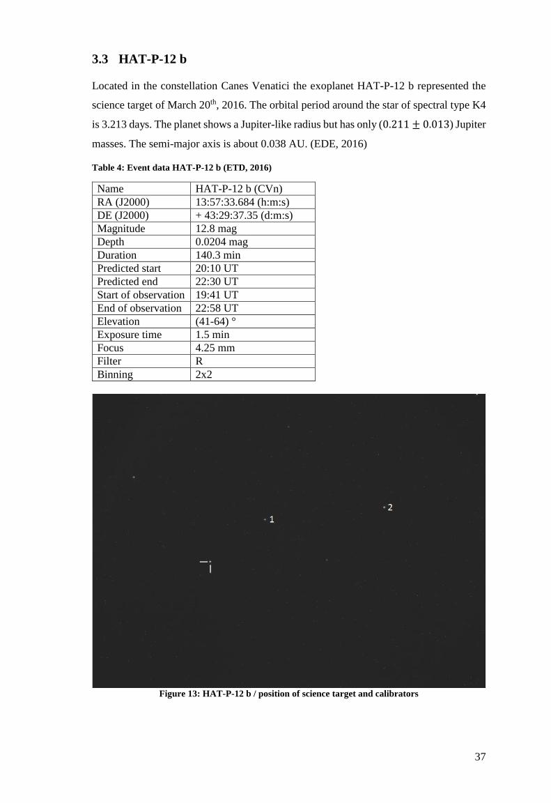
In Figures 11,13,15,16 and 18 the field of view received from the telescope and registered

by the CCD detector is displayed. The observed science target is indicated by the hori-

zontal and vertical white lines. The calibrators are marked with numbers.

Figure 12: WASP-104 b: flux ratio during transit event

Figure 12 shows the flux ratio between the science target WASP-104 b and the calibrator.

Ideally, the calibrator star shows no variability leading to a constant flux as a reference to

the science target. The transiting exoplanet disturbs this constant ratio (in the above figure

normalized) resulting in the dip in the light curve. On the x-axis the time in minutes that

has passed since midnight is shown and the flux ratio is presented on the y-axis. Each flux

measurement is marked with a star symbol. The upper horizontal, dashed line indicates

the normalized lux ratio. The lower dashed line serves as a guideline in order to make it

35

easier to determine the decrease in flux. The two vertical, dashed lines mark the predicted

start and end of the transit. In the field of view there are more stars visible than the science

target and one calibrator. The reason why those are not dealt with as calibrators is that a

calibrator is required to be similar in flux to the observed star. Most of the stars are fainter

and therefore unsuitable for the analysis. Stars brighter than the science target often fall

in the non-linear regime of the camera or are even saturated.

With regard to the exoplanet WASP-104 b, the weather conditions allowed an undis-

turbed observation reflected in the significantly visible transit in the light curve. A com-

putational defect in the automated tracking system of the dome represented the only and

minor problem during the transit event, making manual adjustments of the dome neces-

sary.

This monitoring results in a measured transit depth of about 1.5 %. It is assumed that prior

to and after the transit the flux ratio is F2 = 0.995 and at the lowest point it is F1 = 0.980.

The flux is associated with the apparent magnitude prior and during the transit as follows:

m1 −m2 = −2.5 log (F1F2) ( 13 )

−2.5 log (0.980

0.995) = 0.0165 mag ( 14 )

In this case the calculated difference in apparent magnitude matches the predicted depth

of 0.0158 mag by the Czech Exoplanet Transit Database (ETD) quite nicely. This result

shows clearly that small differences in magnitude are very similar to the relative decrease

in flux.

The radius of host star WASP-104 is R∗ = (0.963 ± 0.027) Rsol (EDE, 2016). By using

Formula ( 8 ), the radius of the transiting planet is calculated in the following way:

RP = √∆F

FR∗2 = √

0.015

0.995∙ (0.963 RSol)2 = 0.118 RSol ( 15 )

To get a first impression of the errors, the Gaussian error propagation was applied:

∆RP = √(|∂RP∂R∗

| ∙ ∆𝑅∗)2

= √∆F

F∙ ∆R∗ = 0.003 RSol ( 16 )

The density is then derived with the known mass of the planet with ρP =3MP

4πRP3 .

ρP =3 ∙ 1.272 MJup

4π ∙ (0.118 RSol)3= 1042 kg/m3 ( 17 )

36

∆ρP = √(|∂ρP𝜕𝑅𝑃

| ∙ ∆𝑅𝑃)2

+ (|∂ρP𝜕𝑀𝑃

| ∙ ∆𝑀𝑃)2

( 18 )

= √(|−9 ∙ MP

4π ∙ RP4 | ∙ ∆𝑅𝑃)

2

+ (|3

4π ∙ RP3 | ∙ ∆𝑀𝑃)

2

= 88 kg/m3

𝑅𝑃 = 0.118 𝑅𝑆𝑜𝑙 , 𝛥𝑅𝑃 = 0.003 𝑅𝑆𝑜𝑙, 𝑀𝑃 = 1.272 𝑀𝑗𝑢𝑝, 𝛥𝑀𝑃 = 0.047 𝑀𝐽𝑢𝑝

Compared to the data offered by NASA Exoplanet Archive, the generated planetary ra-

dius and density fall within the uncertainties. The expected values for those properties are

RP = (0.117 ± 0.004) RSol and ρP = (1074 ± 88) kg/m3. This observation results in

RP = (0.118 ± 0.003) RSol and ρP = (1042 ± 88) kg/m3.

By analysing the light curve, the estimated duration is 105 min, from 1210 min to 1315

min since midnight. Both, the duration and the depth, correspond well to the predicted

data by ETD. The start and end of this observation is merely shifted 5 min forward.

When using Equation ( 12 ) with the measured and known data, the inclination of the

planetary trajectory is easy to obtain:

𝑖 = cos−1

(

√(𝑅𝑃 + 𝑅∗)2 − (sin (

𝜋𝑡𝑃 ) ∙ 𝑎)

2

𝑎

)

= 83.46° ( 19 )

𝑖𝑚𝑎𝑥 = cos−1

(

√(𝑅𝑃 − 𝛥𝑅𝑃 + 𝑅∗ − 𝛥𝑅∗)2 − (sin (

𝜋𝑡𝑃 ) ∙ 𝑎)

2

𝑎

)

= 83.89° ( 20 )

𝛥𝑖 = 𝑖𝑚𝑎𝑥 − 𝑖 = 0.43° ( 21 )

𝑅𝑃 = 0.118 𝑅𝑆𝑜𝑙 , 𝑅∗ = 0.963 𝑅𝑆𝑜𝑙 , 𝑡 = 105 𝑚𝑖𝑛, 𝑃 = 1.755 𝑑𝑎𝑦𝑠, 𝑎 = 0.029 𝐴𝑈

In this case the uncertainty of the inclination was estimated using the min-max estimate

method, just because it is much more convenient than the Gaussian error propagation.

The corresponding value in literature is 𝑖 = (83.63 ± 0.25)°. The calculation results in

𝑖 = (83.46 ± 0.43)° which represents a satisfactory solution.

It has been proved that the exoplanet WASP-104 b can be detected by using the transit

method and the data given by ETD and the NASA Exoplanet Archive could be repro-

duced in an adequate manner.

37

3.3 HAT-P-12 b

Located in the constellation Canes Venatici the exoplanet HAT-P-12 b represented the

science target of March 20th, 2016. The orbital period around the star of spectral type K4

is 3.213 days. The planet shows a Jupiter-like radius but has only (0.211 ± 0.013) Jupiter

masses. The semi-major axis is about 0.038 AU. (EDE, 2016)

Table 4: Event data HAT-P-12 b (ETD, 2016)

Name HAT-P-12 b (CVn)

RA (J2000) 13:57:33.684 (h:m:s)

DE (J2000) + 43:29:37.35 (d:m:s)

Magnitude 12.8 mag

Depth 0.0204 mag

Duration 140.3 min

Predicted start 20:10 UT

Predicted end 22:30 UT

Start of observation 19:41 UT

End of observation 22:58 UT

Elevation (41-64) °

Exposure time 1.5 min

Focus 4.25 mm

Filter R

Binning 2x2

Figure 13: HAT-P-12 b / position of science target and calibrators

38

Figure 14: HAT-P-12 b: flux ratio during transit event

Figure 14 shows the flux ratio between the science target HAT-P-12 b and the two cali-

brators. Each measured flux ratio is marked with a star or diamond symbol according to

the used calibrator. Again, the two vertical, dashed lines mark the predicted start and end

of the transit. This time more than one calibrator is used in order to generate another light

curve to improve and to check the data.

The weather seemed to be acceptable for a transit observation but unfortunately towards

the end of the observation cirrus clouds and low stratus appeared. Moon light might have

been reflected at the clouds leading to even more unfavourable conditions. The weather

change might explain the noisy light curve at the end of the predicted transit. Worth men-

tioning as well is the fact that the dome had to be manually adjusted causing a potential

shadowing of the telescope. Nevertheless, the depth can be determined to be 2.5 %

(F1 = 0.965, F2 = 0.990). Furthermore, the difference in the apparent magnitude is

given as follows:

−2.5 log (0.965

0.990) = 0.0278 mag ( 22 )

In this case the calculated difference in apparent magnitude differs from the predicted

depth of 0.0204 mag (ETD). A possible explanation could be found in the strangely dis-

tributed measurement at the end of the observation. Therefore, the determination of a flux

value was difficult.

The radius of host star HAT-P-12 is R∗ = (0.701 ± 0.017) Rsol (EDE, 2016). The radius

of the transiting planet is calculated in the following way:

RP = √0.025

0.990∙ (0.701 RSol)2 = 0.111 RSol ( 23 )

∆RP = √(|∂RP∂R∗

| ∙ ∆𝑅∗)2

= √∆F

F∙ ∆R∗ = 0.003 RSol ( 24 )

39

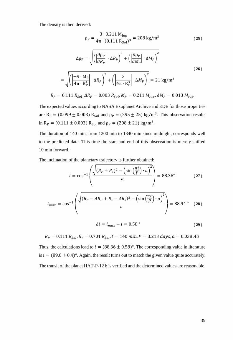
The density is then derived:

ρP =3 ∙ 0.211 MJup

4π ∙ (0.111 RSol)3= 208 kg/m3 ( 25 )

∆ρP = √(|∂ρP𝜕𝑅𝑃

| ∙ ∆𝑅𝑃)2

+ (|∂ρP𝜕𝑀𝑃

| ∙ ∆𝑀𝑃)2

( 26 )

= √(|−9 ∙ MP

4π ∙ RP4 | ∙ ∆𝑅𝑃)

2

+ (|3

4π ∙ RP3 | ∙ ∆𝑀𝑃)

2

= 21 kg/m3

𝑅𝑃 = 0.111 𝑅𝑆𝑜𝑙 , 𝛥𝑅𝑃 = 0.003 𝑅𝑆𝑜𝑙, 𝑀𝑃 = 0.211 𝑀𝑗𝑢𝑝, 𝛥𝑀𝑃 = 0.013 𝑀𝐽𝑢𝑝

The expected values according to NASA Exoplanet Archive and EDE for those properties

are RP = (0.099 ± 0.003) RSol and ρP = (295 ± 25) kg/m3. This observation results

in RP = (0.111 ± 0.003) RSol and ρP = (208 ± 21) kg/m3.

The duration of 140 min, from 1200 min to 1340 min since midnight, corresponds well

to the predicted data. This time the start and end of this observation is merely shifted

10 min forward.

The inclination of the planetary trajectory is further obtained:

𝑖 = cos−1

(

√(𝑅𝑃 + 𝑅∗)2 − (sin (

𝜋𝑡𝑃 ) ∙ 𝑎)

2

𝑎

)

= 88.36° ( 27 )

𝑖𝑚𝑎𝑥 = cos−1

(

√(𝑅𝑃 − 𝛥𝑅𝑃 + 𝑅∗ − 𝛥𝑅∗)

2 − (sin (𝜋𝑡𝑃 ) ∙ 𝑎)

2

𝑎

)

= 88.94 ° ( 28 )

𝛥𝑖 = 𝑖𝑚𝑎𝑥 − 𝑖 = 0.58 ° ( 29 )

𝑅𝑃 = 0.111 𝑅𝑆𝑜𝑙 , 𝑅∗ = 0.701 𝑅𝑆𝑜𝑙 , 𝑡 = 140 𝑚𝑖𝑛, 𝑃 = 3.213 𝑑𝑎𝑦𝑠, 𝑎 = 0.038 𝐴𝑈

Thus, the calculations lead to 𝑖 = (88.36 ± 0.58)°. The corresponding value in literature

is 𝑖 = (89.0 ± 0.4)°. Again, the result turns out to match the given value quite accurately.

The transit of the planet HAT-P-12 b is verified and the determined values are reasonable.

40

3.4 EPIC-211089792 b

Also known as K2-29 b or WASP-152 b, this exoplanet orbits in 3.259 days around a

relatively bright G7 dwarf at a distance of 0.042 AU. It was the target on March 30th,

2016. This planet found in the Taurus constellation resembles Jupiter in radius but has

(0.73 ± 0.04) Jupiter masses. The hot Jupiter’s parent star has a nearby K5V companion

which makes it a binary system. (Santerne et al., 2016)

Table 5: Event data EPIC-211089792 b (ETD, 2016)

Name EPIC-211089792 b (Tau)

RA (J2000) 04:10:40.955 (h:m:s)

DE (J2000) + 24:24:07:35 (d:m:s)

Magnitude 12.526 mag

Depth 0.0215 mag

Duration 133.2 min

Predicted start 18:09 UT

Predicted end 20:22 UT

Start of observation 18:18 UT

End of observation 20:42 UT

Elevation (42-20) °

Exposure time 10x: 1 min

2x: 1.5 min

until 19:45 UT: 2 min

until end: 2.5 min

Focus 4.25 mm

Filter R

Binning 2x2

41

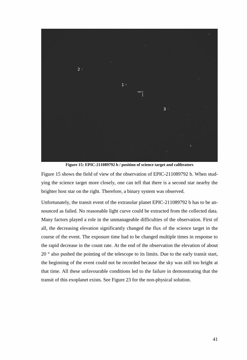
Figure 15: EPIC-211089792 b / position of science target and calibrators

Figure 15 shows the field of view of the observation of EPIC-211089792 b. When stud-

ying the science target more closely, one can tell that there is a second star nearby the

brighter host star on the right. Therefore, a binary system was observed.

Unfortunately, the transit event of the extrasolar planet EPIC-211089792 b has to be an-

nounced as failed. No reasonable light curve could be extracted from the collected data.

Many factors played a role in the unmanageable difficulties of the observation. First of

all, the decreasing elevation significantly changed the flux of the science target in the

course of the event. The exposure time had to be changed multiple times in response to

the rapid decrease in the count rate. At the end of the observation the elevation of about

20 ° also pushed the pointing of the telescope to its limits. Due to the early transit start,

the beginning of the event could not be recorded because the sky was still too bright at

that time. All these unfavourable conditions led to the failure in demonstrating that the

transit of this exoplanet exists. See Figure 23 for the non-physical solution.

42

3.5 XO-1 b

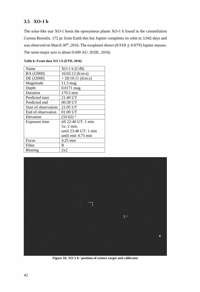
The solar-like star XO-1 hosts the eponymous planet XO-1 b found in the constellation

Corona Borealis. 172 pc from Earth this hot Jupiter completes its orbit in 3.942 days and

was observed on March 30th, 2016. The exoplanet shows (0.918 ± 0.079) Jupiter masses.

The semi-major axis is about 0.049 AU. (EDE, 2016)

Table 6: Event data XO 1 b (ETD, 2016)

Name XO-1 b (CrB)

RA (J2000) 16:02:12 (h:m:s)

DE (J2000) + 28:10:11 (d:m:s)

Magnitude 11.3 mag

Depth 0.0171 mag

Duration 179.5 min

Predicted start 21:40 UT

Predicted end 00:39 UT

Start of observation 21:05 UT

End of observation 01:00 UT

Elevation (33-62) °

Exposure time till 22:40 UT: 1 min

5x: 2 min.

until 23:48 UT: 1 min

until end: 0.75 min

Focus 4.25 mm

Filter R

Binning 2x2

Figure 16: XO-1 b / position of science target and calibrator

43

Figure 17: XO-1 b: flux ratio during transit event

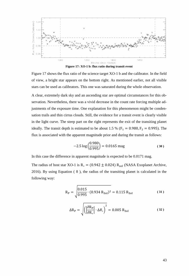
Figure 17 shows the flux ratio of the science target XO-1 b and the calibrator. In the field

of view, a bright star appears on the bottom right. As mentioned earlier, not all visible

stars can be used as calibrators. This one was saturated during the whole observation.

A clear, extremely dark sky and an ascending star are optimal circumstances for this ob-

servation. Nevertheless, there was a vivid decrease in the count rate forcing multiple ad-

justments of the exposure time. One explanation for this phenomenon might be conden-

sation trails and thin cirrus clouds. Still, the evidence for a transit event is clearly visible

in the light curve. The steep part on the right represents the exit of the transiting planet

ideally. The transit depth is estimated to be about 1.5 % (F1 = 0.980, F2 = 0.995). The

flux is associated with the apparent magnitude prior and during the transit as follows:

−2.5 log (0.980

0.995) = 0.0165 mag ( 30 )

In this case the difference in apparent magnitude is expected to be 0.0171 mag.

The radius of host star XO-1 is R∗ = (0.942 ± 0.024) Rsol (NASA Exoplanet Archive,

2016). By using Equation ( 8 ), the radius of the transiting planet is calculated in the

following way:

RP = √0.015

0.995∙ (0.934 RSol)2 = 0.115 RSol ( 31 )

∆RP = √(|∂RP∂R∗

| ∙ ∆𝑅∗)2

= 0.005 RSol ( 32 )

44

The density is further given as:

ρP =3 ∙ 0.918 MJup

4π ∙ (0.115 RSol)3= 812 kg/m3 ( 33 )

∆ρP = √(|∂ρP𝜕𝑅𝑃

| ∙ ∆𝑅𝑃)2

+ (|∂ρP𝜕𝑀𝑃

| ∙ ∆𝑀𝑃)2

= 127 𝑘𝑔/𝑚3 ( 34 )

𝑅𝑃 = 0.115 𝑅𝑆𝑜𝑙 , 𝛥𝑅𝑃 = 0.005 𝑅𝑆𝑜𝑙, 𝑀𝑃 = 0.918 𝑀𝑗𝑢𝑝, 𝛥𝑀𝑃 = 0.079 𝑀𝐽𝑢𝑝

This observation results in RP = (0.115 ± 0.005) RSol and ρP = (812 ± 126) kg/m3.

Compared to the data offered by EDE, the generated planetary radius and density are

acceptable when taking the uncertainty into account. The expected values for those prop-

erties are RP = (0.121 ± 0.005) RSol and ρP = (650 ± 96) kg/m3.

An astonishing fact is the shift in the transit time. This observation suggests a start and

end 15 min prior to the predicted time (from 1285 to 1460 min since midnight). This

results in a duration of 175 min, a difference of 5 min to the data by ETD.

The inclination of the planetary trajectory is calculated below:

𝑖 = cos−1

(

√(𝑅𝑃 + 𝑅∗)2 − (sin (

𝜋𝑡𝑃 ) ∙ 𝑎)

2

𝑎

)

= 88.52 ° ( 35 )

𝑖𝑚𝑎𝑥 = cos−1

(

√(𝑅𝑃 − 𝛥𝑅𝑃 + 𝑅∗ − 𝛥𝑅∗)2 − (sin (

𝜋𝑡𝑃 ) ∙ 𝑎)

2

𝑎

)

= 89.36 ° ( 36 )

𝛥𝑖 = 𝑖𝑚𝑎𝑥 − 𝑖 = 0.84 ° ( 37 )

𝑅𝑃 = 0.115 𝑅𝑆𝑜𝑙 , 𝑅∗ = 0.942 𝑅𝑆𝑜𝑙 , 𝑡 = 175 𝑚𝑖𝑛, 𝑃 = 3.942 𝑑𝑎𝑦𝑠, 𝑎 = 0.049 𝐴𝑈

The corresponding value in literature is 𝑖 = (88.8 ± 0.7)° (EDE, 2016). The computation

of the inclination using the data obtained by the observation leads to 𝑖 = (88.52 ± 0.84)°.

Ones more the given value could be replicated satisfactory.

Evidence for the transiting planet XO-1 b has been found and the data offered by EDE

was confirmed.

45

3.6 HAT-P-5 b

On May 5th, 2016 a clear, cloudless sky offered the perfect conditions to observe the

extrasolar planet HAT-P-5 b in the constellation Lyra. 340 pc from Earth, this hot Jupiter

orbits its Sun-like host star in 2.788 days and has (1.060 ± 0.113) Jupiter masses. The

semi-major axis is 0.041 AU. (EDE, 2016)

Table 7: Event data HAT-P-5 b (ETD, 2016)

Name HAT-P-5 b (Lyr)

RA (J2000) 18:17:37.3 (h:m:s)

DE (J2000) + 36:37:16.6 (d:m:s)

Magnitude 12 mag

Depth 0.0142 mag

Duration 175 min

Predicted start 19:50 UT

Predicted end 22:45 UT

Start of observation 19:36 UT

End of observation 23:11 UT

Elevation (31-61) °

Exposure time 1 min

Focus 4.25 mm

Filter R

Binning 2x2

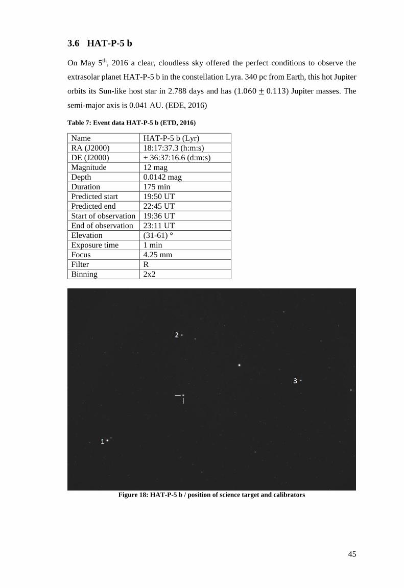
Figure 18: HAT-P-5 b / position of science target and calibrators

46

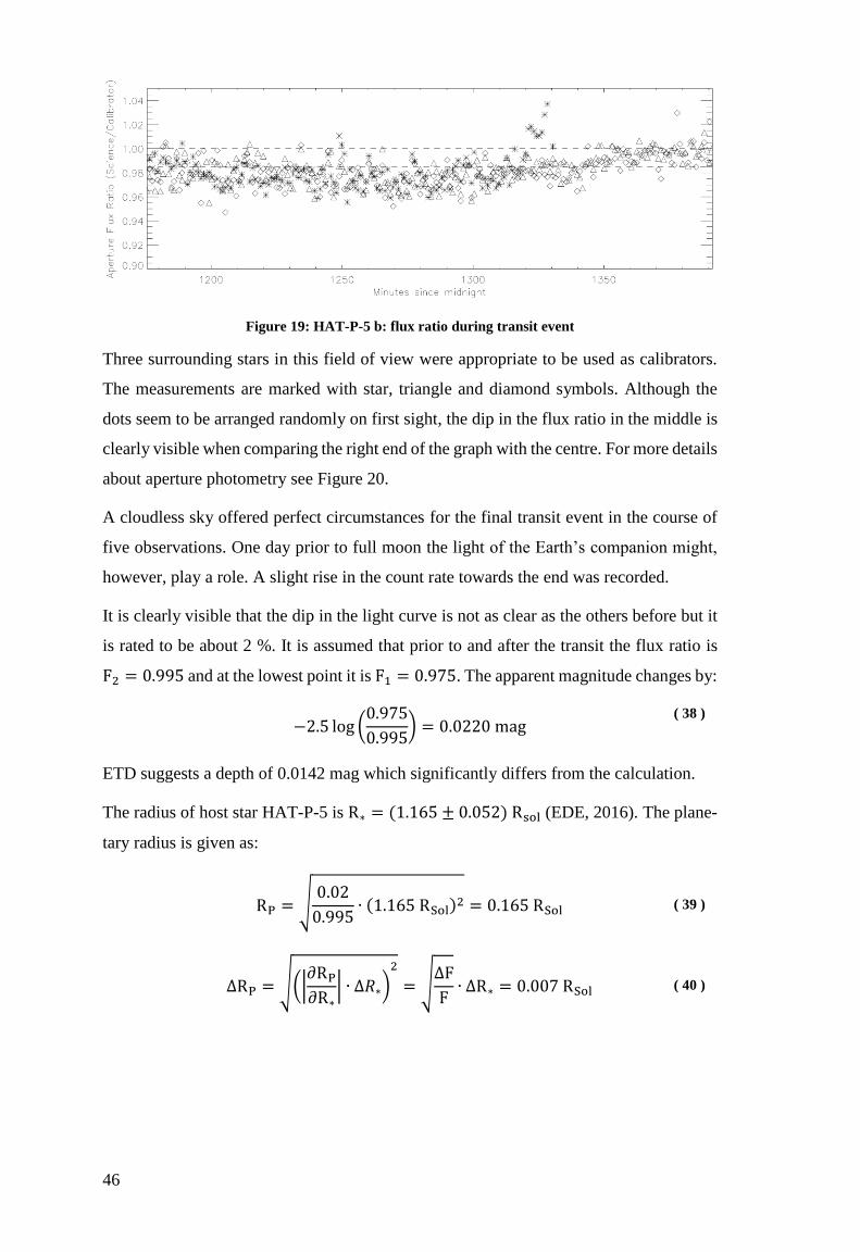
Figure 19: HAT-P-5 b: flux ratio during transit event

Three surrounding stars in this field of view were appropriate to be used as calibrators.

The measurements are marked with star, triangle and diamond symbols. Although the

dots seem to be arranged randomly on first sight, the dip in the flux ratio in the middle is

clearly visible when comparing the right end of the graph with the centre. For more details

about aperture photometry see Figure 20.

A cloudless sky offered perfect circumstances for the final transit event in the course of

five observations. One day prior to full moon the light of the Earth’s companion might,

however, play a role. A slight rise in the count rate towards the end was recorded.

It is clearly visible that the dip in the light curve is not as clear as the others before but it

is rated to be about 2 %. It is assumed that prior to and after the transit the flux ratio is

F2 = 0.995 and at the lowest point it is F1 = 0.975. The apparent magnitude changes by:

−2.5 log (

0.975

0.995) = 0.0220 mag

( 38 )

ETD suggests a depth of 0.0142 mag which significantly differs from the calculation.

The radius of host star HAT-P-5 is R∗ = (1.165 ± 0.052) Rsol (EDE, 2016). The plane-

tary radius is given as:

RP = √0.02

0.995∙ (1.165 RSol)2 = 0.165 RSol ( 39 )

∆RP = √(|∂RP∂R∗

| ∙ ∆𝑅∗)2

= √∆F

F∙ ∆R∗ = 0.007 RSol ( 40 )

47

The density is derived as ρP =3MP

4πRP3.

ρP =

3 ∙ 1.060 MJup

4π ∙ (0.165 RSol)3= 317 kg/m3

( 41 )

∆ρP = √(|∂ρP𝜕𝑅𝑃

| ∙ ∆𝑅𝑃)2

+ (|∂ρP𝜕𝑀𝑃

| ∙ ∆𝑀𝑃)2

= 53 𝑘𝑔/𝑚3 ( 42 )

𝑅𝑃 = 0.165 𝑅𝑆𝑜𝑙 , 𝛥𝑅𝑃 = 0.007 𝑅𝑆𝑜𝑙, 𝑀𝑃 = 1.060 𝑀𝑗𝑢𝑝, 𝛥𝑀𝑃 = 0.113 𝑀𝐽𝑢𝑝

RP = (0.130 ± 0.005) RSol and ρP = (660 ± 120) kg/m3 are the corresponding values

in literature (NASA Exoplanet Archive, 2016). The observation suggests a planetary ra-

dius of RP = (0.165 ± 0.007) RSol and a density of ρP = (317 ± 53) kg/m3.

Due to a late start of the observation it is hard to tell when exactly the graph begins to

decrease. But taking the origin of the light curve at 1175 min since midnight and an esti-

mated end at 1355 min since midnight (180 min in total), there is only a time difference

of 5 min with regard to the predicted duration of 175 min. The observed transit is shifted

10 min forward.

The inclination of the planetary trajectory is calculated by applying Formula ( 12 ):

𝑖 = cos−1

(

√(𝑅𝑃 + 𝑅∗)2 − (sin (

𝜋𝑡𝑃 ) ∙ 𝑎)

2

𝑎

)

= 86.89 ° ( 43 )

𝑖𝑚𝑎𝑥 = cos−1

(

√(𝑅𝑃 − 𝛥𝑅𝑃 + 𝑅∗ − 𝛥𝑅∗)2 − (sin (

𝜋𝑡𝑃 ) ∙ 𝑎)

2

𝑎

)

= 88.14 ° ( 44 )

𝛥𝑖 = 𝑖𝑚𝑎𝑥 − 𝑖 = 1.25 ° ( 45 )

𝑅𝑃 = 0.165 𝑅𝑆𝑜𝑙 , 𝑅∗ = 1.165 𝑅𝑆𝑜𝑙 , 𝑡 = 180 𝑚𝑖𝑛, 𝑃 = 2.788 𝑑𝑎𝑦𝑠, 𝑎 = 0.041 𝐴𝑈

The corresponding value in literature is 𝑖 = (86.75 ± 0.44)° (NASA Exoplanet Archive,

2016). The calculations suggest a value of 𝑖 = (86.89 ± 1.25)° .

A transit of the exoplanet HAT-P-5 b is not questioned. The predicted data could be rep-

licated in an adequate manner.

49

4 Conclusion

Extrasolar planets exist in many variations around different stars. The search for

exoplanets looks back to a rapid progress in theoretical and experimental research. The

number of discovered and later confirmed bodies in diverse systems is continuously

increasing due to a tremendous development of detection methods and instruments.

Compared to our Solar system, some features are also found in extrasolar systems like

planetary types (terrestrial or Jovian) or low eccentricities. In contrary, some conditions

were new to scientists (hot Jupiters). The hunt for an Earth-like planet capable of hosting

some form of life is still a hot topic for researchers and far from being completed.

It is proved that by using the instruments at the observatory Lustbühel in Graz a transit

event can be detected. For four out of five observations it was possible to generate a light

curve indicating a clear dimming in the star’s light due to a transiting planet. Therefore,

the survey was a great success. This technique, however, is quite sensitive to bad condi-

tions like cirrus clouds and moon light. Precise adjustments need to be done to grant the

required precision and reduce any form of uncertainties.

Generally speaking, the data received and further analysed agrees with the predicted val-

ues by either the Exoplanet Transit Database, NASA Exoplanet Archive or Exoplanet

Data Explorer. Reasons for any deviations might be subsequent errors made by analysing

the light curve and further calculating the properties with this data. The instruments are

very sensitive to disturbances generated by for instance weather changes or moon light.

In the previous chapter the determination of the flux ratio prior and during the transit is

estimated by the observer, but is normally fitted with mathematical methods. On the basis

of this value the planetary radius and density as well as the orbital inclination were

computed. Thereby, a previously made error could influence the whole analysis.

50

Table 8: Results of the four successful observations

WASP-104 b HAT-P-12 b

Observation Literature Observation Literature

Depth / mag 0.0165 0.0158 0.0278 0.0204

Duration / min 105 105.72 140 140.3

RP / RSol 0.118 ± 0.003 0.117 ± 0.004 0.111 ± 0.003 0.099 ± 0.003

ρP / kg/m³ 1042 ± 88 1074 ± 88 208 ± 21 295 ± 25

𝑖 / ° 83.5 ± 0.5 83.6 ± 0.3 88.4 ± 0.6 89.0 ± 0.4

XO-1 b HAT-P-5 b

Observation Literature Observation Literature

Depth / mag 0.0165 0.0171 0.0220 0.0142

Duration / min 175 179.5 180 175

RP / RSol 0.115 ± 0.005 0.121 ± 0.005 0.165 ± 0.007 0.130 ± 0.005

ρP / kg/m³ 812 ± 126 650 ± 96 317 ± 53 660 ± 120

𝑖 / ° 88.5 ± 0.9 88.8 ± 0.7 86.9 ± 1.3 86.8 ± 0.5

51

5 List of references

ASA, Cassegrain Telescope (2016). Available online: https://www.optcorp.com/asa-500-

mm-f-9-cassegrain-telescope.html [October 3rd, 2016]

Beaulieu, J.-P. et al. (2006): Discovery of a cool planet of 5.5 Earth masses through

gravitational microlensing. Nature, 439, 437-440.

COROT, Mission (2016). Available online: https://corot.cnes.fr/en/home-56 [October

3rd, 2016]

Cowley, M. & Hughes, S. (2014). Characterization of transiting exoplanets by way of

differential photometry. IOP Publishing Ltd: Physics Education, 49/3.

Deeg, H. (2002). The Transit Method. Available online:

http://www.iac.es/proyecto/tep/transitmet.html [October 3rd, 2016]

ESO Science Release 1245 (2012). Lost in Space: Rogue Planet Spotted?. Available

online: http://www.eso.org/public/news/eso1245/ [October 3rd, 2016]

ETD - Exoplanet Transit Database (2016). Available online: http://var2.astro.cz/ETD/

[October 3rd, 2016]

EDE - Exoplanet Data Explorer (2016). Available online: http://exoplanets.org/ [October

3rd, 2016]

Haswell, C. A. (2010). Transiting Exoplanets. New York: Cambridge University Press

HATNet (2015). Available online: http://hatnet.org/ [October 3rd, 2016]

Hirano, T. (2014). Measurements of Spin-Orbit Angles for Transiting Systems. Tokyo:

Springer Japan

IAU (2006). Resolution B5. Definition of a Planet in the Solar System. Available online:

https://www.iau.org/static/resolutions/Resolution_GA26-5-6.pdf [October 3rd, 2016].

Kepler, NASA Mission (2016). Available online: http://kepler.nasa.gov/ [October 3rd,

2016].

Lammer, H. et al. (2009). What makes a planet habitable?. Astron. Astrophys. Rev. 17,

226-228

Lunine, J. I., Macintosh, B. & Peale S. (2009). The detection and characterization of

exoplanets. Physics Today, 62, 46.

Mason, J. W. (2008). Exoplanets. Detection, Formation, Properties, Habitability.

Chichester: Praxis Publishing Ltd.

Mayor, M. & Queloz, D. (1995). A Jupiter-mass companion to a solar-type star. Nature,

378, 355-359.

NASA Exoplanet Archive (2016). Available online:

http://exoplanetarchive.ipac.caltech.edu/ [October 3rd, 2016].

Perryman, M. (2011). The Exoplanet Handbook. New York: Cambridge University Press.

Piper, S. (2014). Exoplaneten. Die Suche nach einer zweiten Erde. 2nd edition.

Heidelberg: Springer Spektrum.

Santerne, A. et al. (2016). K2-29 b/WASP-152 b: An aligned and inflated hot Jupiter in

a young visual binary. The Astrophysical Journal, Vol. 824, Nr. 1

52

Waldmann, I. (2014). L10: Finding exoplanets with Astrometry and Radial velocities.

Available online: http://zuserver2.star.ucl.ac.uk/~ingo/Lecture_Notes_files/lect10.pdf

[October 3rd, 2016].

WASP, Mission (2014). Available online: http://www.superwasp.org/ [October 3rd,

2016].

Wolszczan, A. & Frail, D. A. (1992). A planetary system around the millisecond pulsar

PSR1257+12. Nature, 355, 145-147

53

6 Appendix

6.1 WASP-104 b

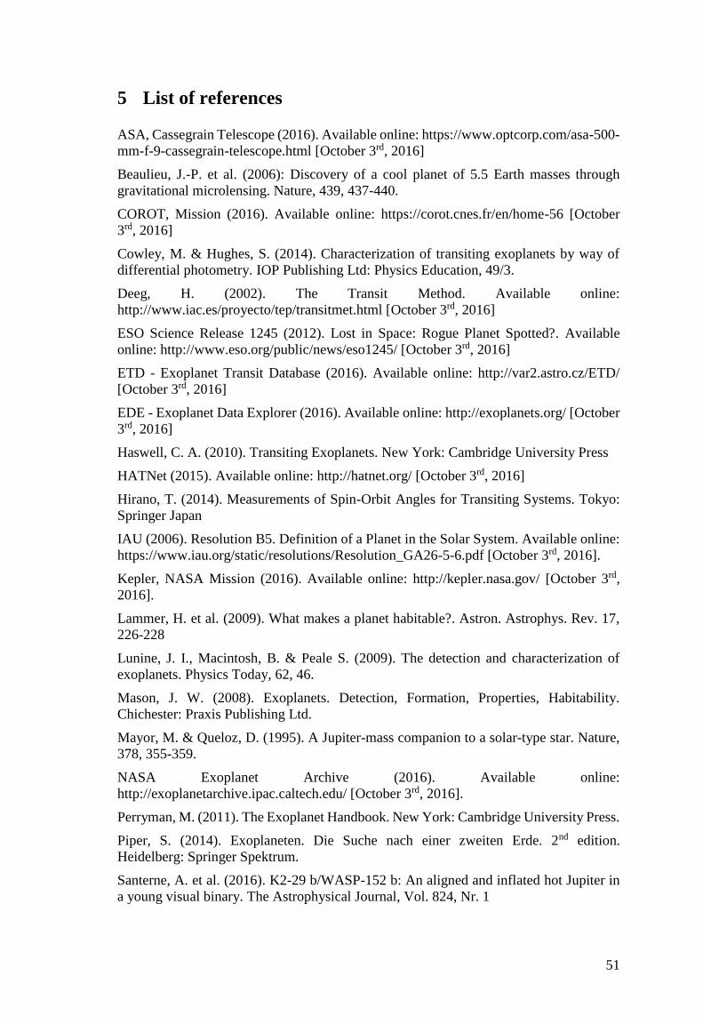
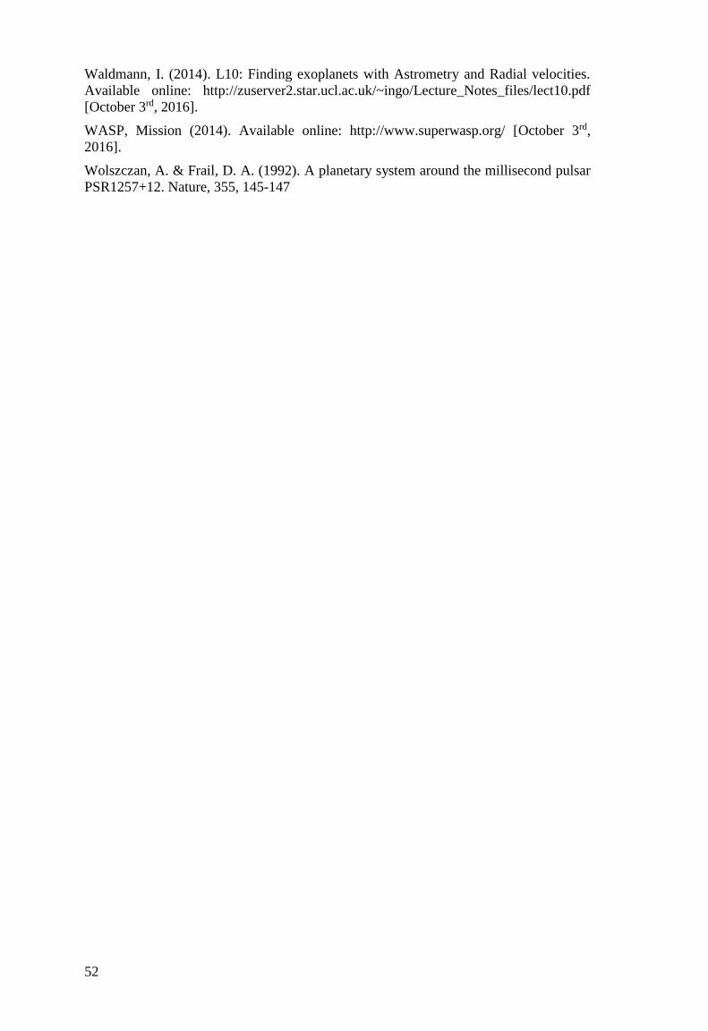
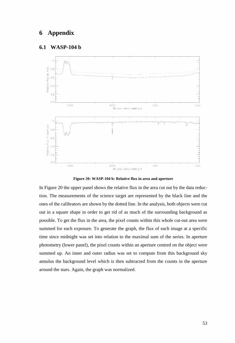
Figure 20: WASP-104 b: Relative flux in area and aperture

In Figure 20 the upper panel shows the relative flux in the area cut out by the data reduc-

tion. The measurements of the science target are represented by the black line and the

ones of the calibrators are shown by the dotted line. In the analysis, both objects were cut

out in a square shape in order to get rid of as much of the surrounding background as

possible. To get the flux in the area, the pixel counts within this whole cut-out area were

summed for each exposure. To generate the graph, the flux of each image at a specific

time since midnight was set into relation to the maximal sum of the series. In aperture

photometry (lower panel), the pixel counts within an aperture centred on the object were

summed up. An inner and outer radius was set to compute from this background sky

annulus the background level which is then subtracted from the counts in the aperture

around the stars. Again, the graph was normalized.

54

6.2 HAT-P-12 b

Figure 21: HAT-P-12 b: Relative flux in area and aperture

For more details, see the description of Figure 20.

6.3 EPIC-211089792 b

Figure 22: EPIC-211089792 b: Relative flux in area and aperture

55

For details, see Figure 20. The relative flux in aperture and area is presented in Figure 22.

The lines vary significantly indicating that something went wrong.

Figure 23: EPIC-211089792 b: flux ratio of star and calibrators during transit event

For a detailed description of the graph, see Figure 12. Unfortunately, it was not possible

to generate a reasonable graph showing the desired dip in the light curve. The plot shows

non-physical solutions.

6.4 XO-1 b

Figure 24: XO-1 b: Relative flux in area and aperture

See Figure 20 for more details concerning the description of the graphs.

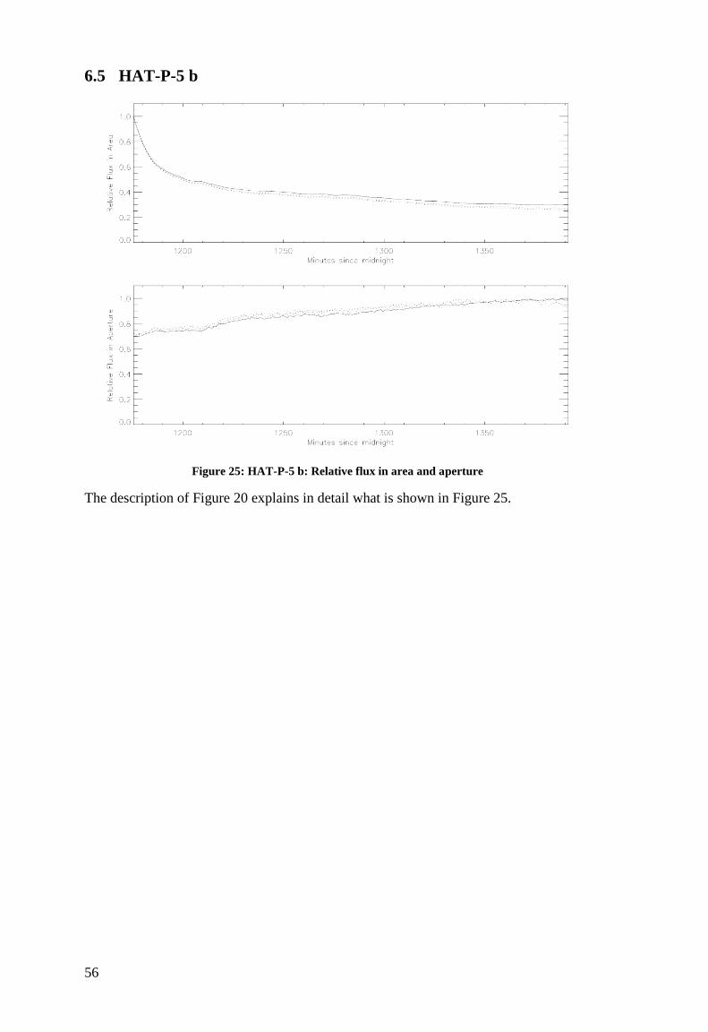
56

6.5 HAT-P-5 b

Figure 25: HAT-P-5 b: Relative flux in area and aperture

The description of Figure 20 explains in detail what is shown in Figure 25.