extremal case of frankl–ray-chaudhuri–wilson inequality

Journal of Statistical Planning andInference 95 (2001) 293–306

www.elsevier.com/locate/jspi

Extremal case of Frankl–Ray-Chaudhuri–Wilson Inequality

Jin Qian ∗, D.K. Ray-ChaudhuriDepartment of Mathematics, The Ohio State University, 100 Math Tower, 231 W 18th Avenue,

Columbus, OH 43210, USA

In honor of S.S. Shrikhande

Abstract

In their 1981 paper, Frankl and Wilson gave a non-uniform analog of Ray-Chaudhuri–WilsonInequality called Frankl–Ray-Chaudhuri–Wilson Inequality. In this paper, we give a completeclassi4cation of the extremal case of their theorem. Our presentation is in the context ofquasi-polynomial semi-lattice which includes the 4nite set case as a special case. c© 2001Elsevier Science B.V. All rights reserved.

MSC: 05C 35

Keywords: Combinatorial inequalities; Quasi-polynomial semi-lattice; L-intersection family;Incidence matrix

1. Introduction

In 1948, de Bruijn and Erd=os (1948) proved the following theorem which probablymarks the beginning of “Combinatorial Inequalities”, an active branch of combinatorics.

Theorem 1. Let S be an n-element set; F⊆P(S). If ∀E �= F ∈F; |E ∩ F |= 1; then|F|6n.

Actually, they also classi4ed the extremal cases, i.e., gave a necessary and suAcientcondition under which the equality holds.Bose (1949) generalized Theorem 1 in the following theorem.

Theorem 2. Let S be an n-element set; F⊆P(S). If there exists a �∈N; such that∀E �= F ∈F; |E ∩ F |= �; then |F|6n.

In the following theorem, Ray-Chaudhuri and Wilson (1975) generalized Theorem 2to multiple intersection sizes. This theorem, which is generally referred to as uniform

∗ Corresponding author.E-mail address: [email protected] (J. Qian).

0378-3758/01/$ - see front matter c© 2001 Elsevier Science B.V. All rights reserved.PII: S0378 -3758(00)00296 -2

294 J. Qian, D.K. Ray-Chaudhuri / J. Statistical Planning and Inference 95 (2001) 293–306

Ray-Chaudhuri–Wilson Inequality or R–W Inequality for short, has become an impor-tant theorem of this subject and inspired many new theorems in this subject.

Theorem 3. Let S be an n-element set; F⊆Pk(S) be a family of subsets of S forsome k ∈N; and L⊆N∪{0} be a :nite set with s elements. If F is an L-intersectionfamily; i.e.; ∀E �= F ∈F; |E ∩ F | ∈L; then |F|6( ns ). The equality holds if and onlyif F is a 2s-design.

More recently, Frankl and Wilson (1981) proved the following analog of R–WInequality. This theorem is referred to in the literature as Frankl–Ray-Chaudhuri–WilsonTheorem.

Theorem 4. Let S be an n-element set; F⊆P(S) be a family of subsets of S; andL⊆N ∪ {0} be a :nite set with s elements. If F is an L-intersection family; i.e.;∀E �= F ∈F; |E ∩ F | ∈L; then |F|6∑s

i=0 (ni ).

This interesting theorem has many proofs. Among them the proof by Alon et al.(1991) is most elegant. In this paper, we are going to give a new proof using “systemof linear equations” method. This was 4rst employed by Ramanan in his wonderfulproof of Frankl–F=uredi conjecture (Ramanan, 2001). In Section 4, we give a com-plete classi4cation of the extremal case. Since we present our results and proofs inthe context of quasi-polynomial semi-lattices which was 4rst introduced by Qian andRay-Chaudhuri (2001) as a general frame work for combinatorial inequalities, we de-vote the next section to a brief introduction to quasi-polynomial semi-lattices.The concept of quasi-polynomial semi-lattices is based on the concept of polynomial

semi-lattices 4rst introduced by Ray-Chaudhuri and Tianbao Zhu (1993).

2. Quasi-polynomial semi-lattices

For any n∈N, we de4ne In = {1; 2; : : : ; n}.Let (X;6) be a 4nite non-empty partially ordered set having the property that (X;6)

is a semi-lattice, i.e., for any x; y∈X there is a unique greatest lower bound of x andy denoted by x ∧ y. We also assume that (X;6) has a height function l(x), wherel(x) + 1 is the number of terms in a maximal chain from the least element, denotedby 0, to the element x including the end elements in the count. Let n be the maximumof l(x) for all x in X . De4ne Xi = {x∈X | l(x) = i}, 06i6n and X0 = {0}. ThenX =

⋃ni=0 Xi is a partition and the subsets Xi’s are called 4bers. The integer n is said

to be the height of (X;6).

De�nition. (X;6) is called a quasi-polynomial semi-lattice if the following three con-ditions hold:

(a) There are n+ 1 integers m0; m1; : : : ; mn such that 06m0¡m1¡ · · ·¡mn.

J. Qian, D.K. Ray-Chaudhuri / J. Statistical Planning and Inference 95 (2001) 293–306 295

(b) There exist n + 1 polynomials fi(x); i = 0; 1; : : : ; n; f0(x) = 1 and fi(x) = ci(x −m0)(x−m1) · · · (x−mi−1) for i=1; : : : ; n, where ci’s are positive rational numbers,such that i6j∈ In ∪ {0} and y∈Xj, |{z ∈Xi | z6y}|= fi(mj).

(c) For all i6j6k ∈ In ∪{0} there exist non-negative integers fijk such that |{z ∈Xj |x6z6y}|=fijk for any x∈Xi; y∈Xk with x6y. Here and in the rest of the paperwe denote {1; 2; : : : ; n} by In.

In the rest of the paper, we call f0; f1; : : : ; fn the associated polynomials of thesemi-lattice and denote |{z ∈Xi | z6y}| by fij(y) for y∈Xj. We write fij for fij(y)when fij(y) does not depend on y.The following remark and notations will be useful in the proofs of some theorems

below.

Remark. It is clear that if F1; F2 ∈X; {E ∈Xi |E6F1; E6F2}= {E ∈Xi |E6F1 ∧F2}.From (b) of the de4nition, we conclude that {E ∈Xi |E6F1; E6F2}|={E ∈Xi |E6F1∧F2}|= fi(|F1 ∧ F2|). Here |F | is de4ned to be ml for any F ∈Xl with l(F) = l.

The following are examples of quasi-polynomial semi-lattices which are also impor-tant combinatorial objects.Examples:

(1) Johnson scheme. Let V be an n-element set and Xi be the set of all i-elementsubsets of V; 06i6n. Then X =

⋃ni=0 Xi, with inclusion as the partial order, is a

semi-lattice. Let mi = i; fi(x) = (xi ), a polynomial of degree i in the variable x. It

is easy to see that (X;6) is a quasi-polynomial semi-lattice.(2) q-Analogue of Johnson scheme. Let V be an n-dimensional vector space over a

4nite 4eld GF(q), Xi be the set of all i-dimensional subspaces of V , 06i6n. Letmi= qi; fi(x)= [

xi ]q, a polynomial of degree i in the variable x. Then X =

⋃ni=0 Xi

is a quasi-polynomial semi-lattice with inclusion as the partial order.(3) Hamming scheme. Let W be an s-element set, where s is a positive integer. We

de4ne Xi={(L; h) |L⊆{1; 2; : : : ; n}; |L|= i; h :L→ W a map}; 16i6n; X0={∅},where ∅ is taken to be the least element, and X = ⋃n

i=0 Xi: (L1; h1)6(L2; h2) ifand only if L1⊆L2, and h2|L1 =h1. Then (X;6) is a quasi-polynomial semi-lattice,with mi = i; fi(x) = (

xi ).

(4) q-Analogue of Hamming scheme. Let V be an n-dimensional vector space overa 4nite 4eld GF(q) and W be an s-dimensional vector space over a 4nite 4eldGF(q). De4ne Xi={(U; h) |U⊆V; dim(U )=i; h :U→W , a linear transformation},06i6n. Let X =

⋃ni=0 Xi: ∀(U1; h1); (U2; h2)∈X , de4ne (U1; h1)6(U2; h2) if and

only if U1⊆U2 and h2|U1 = h1. Then (X;6) is a quasi-polynomial semi-lattice,with mi = qi; fi(x) = [

xi ]q.

(5) Ordered design. Let W be an s-element set and V be an n-element set with n6s.We de4ne Xi={(L; h) |L⊆V; |L|= i; h :L→ W an injection}, 16i6n; X0 ={0},where 0 is taken as the least element, and X =

⋃ni=0 Xi: ∀(L1; h1); (L2; h2)∈X ,


de4ne (L1; h1)6(L2; h2) if and only if L1⊆L2 and h2|L1 = h1. Then (X;6) is aquasi-polynomial semi-lattice, with mi = i; fi(x) = (

xi ).

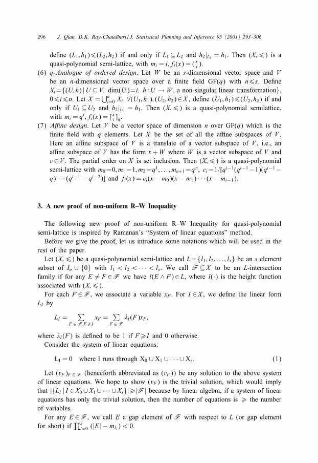
(6) q-Analogue of ordered design. Let W be an s-dimensional vector space and Vbe an n-dimensional vector space over a 4nite 4eld GF(q) with n6s. De4neXi={(U; h) |U ⊆V; dim(U )=i; h :U → W , a non-singular linear transformation},06i6n. Let X =

⋃ni=0 Xi: ∀(U1; h1); (U2; h2)∈X , de4ne (U1; h1)6(U2; h2) if and

only if U1⊆U2 and h2|U1 = h1. Then (X;6) is a quasi-polynomial semilattice,with mi = qi; fi(x) = [

xi ]q.

(7) A<ne design. Let V be a vector space of dimension n over GF(q) which is the4nite 4eld with q elements. Let X be the set of all the aAne subspaces of V .Here an aAne subspace of V is a translate of a vector subspace of V , i.e., anaAne subspace of V has the form v+W where W is a vector subspace of V andv∈V . The partial order on X is set inclusion. Then (X;6) is a quasi-polynomialsemi-lattice with m0=0; m1=1; m2=q1; : : : ; mn+1=qn; ci=1=[qi−1(qi−1−1)(qi−1−q) · · · (qi−1 − qi−2)] and fi(x) = ci(x − m0)(x − m1) · · · (x − mi−1).

3. A new proof of non-uniform R–W Inequality

The following new proof of non-uniform R–W Inequality for quasi-polynomialsemi-lattice is inspired by Ramanan’s “System of linear equations” method.Before we give the proof, let us introduce some notations which will be used in the

rest of the paper.Let (X;6) be a quasi-polynomial semi-lattice and L={l1; l2; : : : ; ls} be an s element

subset of In ∪ {0} with l1¡l2¡ · · ·¡ls. We call F⊆X to be an L-intersectionfamily if for any E �= F ∈F we have l(E ∧ F)∈L, where l(·) is the height functionassociated with (X;6).For each F ∈F, we associate a variable xF . For I ∈X , we de4ne the linear formLI by

LI =∑

F ∈F;F¿IxF =

∑F ∈F

�I (F)xF ;

where �I (F) is de4ned to be 1 if F¿I and 0 otherwise.Consider the system of linear equations:

-LI = 0 where I runs through X0 ∪ X1 ∪ · · · ∪ Xs: (1)

Let (vF)F ∈F (henceforth abbreviated as (vF)) be any solution to the above systemof linear equations. We hope to show (vF) is the trivial solution, which would implythat |{LI | I ∈X0 ∪X1 ∪ · · · ∪Xs}|¿|F| because by linear algebra, if a system of linearequations has only the trivial solution, then the number of equations is ¿ the numberof variables.For any E ∈F, we call E a gap element of F with respect to L (or gap element

for short) if∏si=0 (|E| − mli)¡ 0.


The following theorem is a generalization of Theorem 4 to quasi-polynomial semi-lattice.

Theorem 5. Let (X;6) be a quasi-polynomial semi-lattice; L⊆ In ∪ {0} with |L|= s.If F is an L-intersection family; then |F|6|X0|+ |X1|+ · · ·+ |Xs|.

Proof. As remarked before, it is enough to show that (vE) = 0 is the only solution of(1), where 0 is the all 0 vector in R|F|. Suppose on the contrary, (vE) �= 0. De4neJ = {l(E) |E ∈F; vE �= 0} and let j0 be the largest number in J . So there existsE0 ∈F, such that l(E0) = j0 and vE0 �= 0. Let

f(x) =∏

li¡j0 ;li ∈ L(x − mli)

whose degree is denoted by d. Since f0; f1; : : : ; fd form a basis for the space of allthe polynomials of degree 6d, there exists c0; c1; : : : ; cd such that c0f0 + c1f1 + · · ·+cdfd = f(x), where fi’s are the associated polynomials of the semi-lattice. We nowshow that

d∑i=0ci

∑I ∈ XiLI �I (E0) =

∑E ∈F

f(|E ∧ E0|)xE:

In fact, both sides of the above equation are linear forms in xE’s. The coeAcient ofthe xE on the left-hand side is

∑di=0 fi(|E ∧ E0|) = f(|E ∧ E0|) which is equal to that

of the right-hand side. For more detail, see Lemma 3 in the next section.Specializing xE = vE; ∀E ∈F, we have

d∑i=0ci

∑I ∈ XiLI ((vE))�I (E0) =

∑E ∈F

f(|E ∧ E0|)vE: (2)

Let us consider the right-hand side (RHS) of the above equation. If E ∈F, l(E)6j0and E �= E0, then l(E∧E0)¡l(E0)=j0 and so f(|E∧E0|)=0; if E ∈F and l(E)¿j0,then by the de4nition of J and j0, vE =0. Overall, the right-hand side of the above isequal to f(|E0 ∧ E0|)vE0 = f(mj0 )vE .The left-hand side of (2), however is equal to zero because LI ((vE)) = 0 for allI ∈X0 ∪ X1 ∪ · · · ∪ Xs and d6s by the de4nition of d. So 0 = f(mj0 )vE and we getvE0 =0 since f(mj0 ) �= 0 by the de4nition of f. This contradiction completes the proof.

4. The extremal case of non-uniform R–W Theorem

Theorem 6. Let (X;6) be a quasi-polynomial semi-lattice; L∈ In ∪ {0} be an s-set.If F is an L-intersection family; then |F| = |X0| + |X1| + · · · + |Xs| if and only ifL= {0; 1; : : : ; s− 1} and F= X0 ∪ X1 ∪ · · · ∪ Xs.

The proof of this theorem is divided into seven lemmas. The 4rst three lemmasare auxiliary lemmas. Among the seven lemmas, Lemmas 2 and 7 are due to Qian


and Ray-Chaudhuri (1997), Lemmas 3 and 4 are due to Ramanan (2001). They areincluded here for the convenience of the reader.

Lemma 1. If x1; x2; : : : ; xs be s distinct non-negative integers and {x1; x2; : : : ; xs} �={0; 1; : : : ; s− 1}; then

f0(mx1 ) f1(mx1 ) · · · fs−2(mx1 ) fs(mx1 )f0(mx2 ) f1(mx2 ) · · · fs−2(mx2 ) fs(mx2 )· · · · · · · · · · · · · · ·f0(mxs) f1(mxs) · · · fs−2(mxs) fs(mxs)

is non-singular.

Proof. First we prove the following:

Claim. For any s variables x1; x2; : : : ; xs;

∣∣∣∣∣∣∣∣∣

1 x1 · · · xs−21 xs11 x2 · · · xs−22 xs2.........

......

1 xs · · · xs−2s xss

∣∣∣∣∣∣∣∣∣=

∣∣∣∣∣∣∣∣∣

1 x1 · · · xs−111 x2 · · · xs−12.........

...1 xs · · · xs−1s

∣∣∣∣∣∣∣∣∣(x1 + x2 + · · ·+ xs):

Proof. We denote the left-hand side by W and the van de Monte determinant on theright-hand side by V . It is obvious that W;V ∈Q[x1; x2; : : : ; xs], the polynomial ringgenerated by s variables x1; x2; : : : ; xs. If xi = xj in W , then W = 0 which shows that(xi − xj) |W for any i �= j = 1; 2; : : : ; s. Since V =∏

16i¡j6s (xj − xi). We have Vdivides W . Let us consider W=V . Since W; V are obviously homogeneous polynomialsand degW = 1 + degV . So W=V is a polynomial of 4rst degree in Q[x1; x2; : : : ; xs]. Itis also clear that for any permutation ! of {1; 2; : : : ; s}; (W=V )(x!(1); x!(2); : : : ; x!(s)) =(W=V )(x1; x2; : : : ; xs). So (W=V )(x1; x2; : : : ; xs) = c(x1 + x2 + · · ·+ xs) for some constantc∈Q. We order the monomials in Q[x1; x2; : : : ; xs] lexicographically. Forexample, xi11 x

i22 · · · xiss � xj11 xj22 · · · xjss if and only if for some integer t; 16t6s such that

i1=j1; : : : ; it−1=jt−1 and it ¿ jt . It is clear that the leading term of W is (−1)s+1xs1 : : : ;and the leading term of V is (−1)s+1xs−11 : : :, so the leading term of W=V is x1, i.e.,c = 1. This proves the claim.

We let v=m0 +m1 + · · ·+ms−1 and B be the above matrix . It is clear that ∃c �= 0,such that

c det(B) =

∣∣∣∣∣∣∣∣

1 mx1 · · · ms−2x1 msx1 − vms−1x11 mx2 · · · ms−2x2 msx2 − vms−1x2· · · · · · · · · · · · · · ·1 mxs · · · ms−2xs msxs − vms−1xs

∣∣∣∣∣∣∣∣


=

∣∣∣∣∣∣∣∣

1 mx1 · · · ms−2x1 msx11 mx2 · · · ms−2x2 msx2· · · · · · · · · · · · · · ·1 mxs · · · ms−2xs msxs

∣∣∣∣∣∣∣∣− v

∣∣∣∣∣∣∣∣

1 mx1 · · · ms−2x1 ms−1x11 mx2 · · · ms−2x2 ms−1x2· · · · · · · · · · · · · · ·1 mxs · · · ms−2xs ms−1xs

∣∣∣∣∣∣∣∣

= (mx1 + mx2 + · · ·+ mxs − v)

∣∣∣∣∣∣∣∣

1 mx1 · · · ms−2x1 ms−1x11 mx2 · · · ms−2x2 ms−1x2· · · · · · · · · · · · · · ·1 mxs · · · ms−2xs ms−1xs

∣∣∣∣∣∣∣∣:

Since x1; x2; : : : ; xs are s distinct non-negative integers and {x1; x2; : : : ; xs} �= {0; 1; : : : ;s − 1}; mx1 + mx2 + · · · + mxs ¿m0 + m1 + · · · + ms−1 = v. So c det(B) �= 0, whichimplies that B is non-singular.

Lemma 2. Let (X;6) be a quasi-polynomial semi-lattice. For any s positive integers$1; $2; : : : ; $s ∈{1; 2; : : : ; n} and any j such that 06j¡$1; there exist positive rationalnumbers d0; d1; : : : ; ds such that

s∑i=0(−1)idi(x − mj)(x − mj+1) · · · (x − mj+i−1)

= (−1)s(x − m$1 )(x − m$2 ) · · · (x − m$s):

(The term for i = 0 on the left-hand side of the above is (−1)0d0 by convention.)

Proof. We induct on s. When s= 1, it is trivially true. Suppose it holds for s.Next, we prove that the lemma holds for s+ 1.

(−1)s+1(x − m$1 )(x − m$2 ) · · · (x − m$s+1)

= (−1)(x − m$1 )[(−1)s(x − m$2 ) · · · (x − m$s+1)]

= (−1)[(x − mj)− (m$1 − mj)][(−1)s(x − m$2 ) · · · (x − m$s+1)]

= I + II; (3)

where I= (−1)(x−mj)[(−1)s(x−m$2 ) · · · (x−m$s+1)] and II= (m$1 −mj)[(−1)s(x−m$2 ) · · · (x − m$s+1)].Since j + 1¡$1 + 16$2, we can apply induction hypothesis to I and we have

I= (−1)(x − mj)s∑i=0(−1)iui(x − mj+1) · · · (x − mj+1+i−1)

=s∑i=0(−1)i+1ui(x − mj)(x − mj+1) · · · (x − mj+1+i−1)

for some positive rational numbers us; us−1; : : : ; u0.


Using induction hypothesis on II, we have

II= (m$1 − mj)s∑i=0(−1)ivi (x − mj) · · · (x − mj+i−1)

=s∑i=0(−1)i(m$1 − mj)vi(x − mj) · · · (x − mj+i−1)

for some positive rational numbers vs; vs−1; : : : ; v0.Adding up I and II, we have

(−1)(x − mj)[(−1)s(x − m$2 ) · · · (x − m$s+1)]

+ (m$1 − mj)[(−1)s(x − m$2 ) · · · (x − m$s+1)]

=s+1∑i=0(−1)idi(x − mj) · · · (x − mj+i−1);

where

ds+1 = us,ds = us−1 + (m$1 − mj)vs,ds−1 = us−2 + (m$1 − mj)vs−1,...d0 = (m$1 − mj)v0.

So ds+1; ds; : : : ; d0 are positive since $1¿j and m$i − mj ¿ 0 by the de4nition ofthe quasi-polynomial semi-lattice. This proves the lemma.

Corollary 1. Let (X;6) be a quasi polynomial semilattice; s a positive integer withs6n and l1; l2; : : : ; ls be s integers in {0; 1; 2; : : : ; n} with {l1; l2; : : : ; ls} �= {0; 1; : : : ;s − 1}. There exist s + 1 non-negative rational numbers b0; b1; : : : ; bs with bs−1¿ 0and bs ¿ 0 such that

s∑i=0(−1)ibifi(x) = (−1)s(x − ml1 )(x − ml2 ) · · · (x − mls):

Proof. WLOG, we suppose l1¡l2¡ · · ·¡ls. We 4rst prove the corollary when l1=0.We let u be the largest integer such that l1 = 0, l2 = 1; : : : ; lu = u − 1. Since

{l1; l2; : : : ; ls} �= {0; 1; : : : ; s − 1}, we have 0¡u¡s. Note that u¡lu+1. ApplyingLemma 2 with j = u and lu+1 as l1, there exist positive integers du; du+1; : : : ; dswith

(−1)s−u(x − mlu+1)(x − mlu+2) · · · (x − mls)

=s−u∑i=0(−1)idu+i(x − mu)(x − mu+1) · · · (x − mu+i−1):


Now, we multiply it by (−1)u(x − m0)(x − m1) · · · (x − mu−1) (which is equal to(−1)u(x − ml1 )(x − ml2 ) · · · (x − mlu) by the de4nition of u) and we have

(−1)s(x − ml1 )(x − ml2 ) · · · (x − mls)=s−u∑i=0(−1)i+udu+i(x − m0)(x − m1) · · · (x − mu+i−1)

=s∑i=0(−1)idi(x − m0)(x − m1) · · · (x − mi−1);

where d0 = d1 = · · ·= du−1 = 0. By the de4nition of quasi-polynomial semi-lattice, wehave

(−1)s(x − ml1 )(x − ml2 ) · · · (x − mls) =s∑i=0(−1)ibifi(x);

here bi = di=ci; i= 0; 1; : : : ; n; ci’s are the positive constants associated with the quasi-polynomial semi-lattice. Note that bs−1 = ds−1=cs−1¿ 0 and bs = ds=cs ¿ 0. This com-pletes the proof of corollary when l1 = 0. The proof of the case when l1 �= 0 can bedone similarly by applying Lemma 2 with j = 0.

Lemma 3. We keep the same notation as in Theorem 6 and Corollary 1. If we letg(x) = (x − ml1 )(x − ml2 ) · · · (x − mls); then we have:

s∑i=0(−1)ibi

∑I ∈ XiL2I =

∑E ∈F

(−1)sg(|E|)x2E: (4)

Proof. We regard both sides as quadratic forms on xE’s, E ∈F and try to show thatthe corresponding coeAcients are equal.For example, for E �= F ∈F, the term L2I contributes a term 2xExF if and only ifI6E∧F . Therefore, the coeAcient of xExF on the LHS of (4) is 2

∑si=0 (−1)ibifi(|E∧

F |) (see the remark in Section 2 after the de4nition of quasi-polynomial semi-lattice)which is equal to 2(−1)s(|E∧F |−ml1 )(|E∧F |−ml2 ) · · · (|E∧F |−mls) by Corollary 1.Since F is an L-intersection family with L={l1; l2; : : : ; ls}; |E∧F | ∈ {ml1 ; ml2 ; : : : ; mls}and so the product in the previous sentence is 0. Obviously, the coeAcient of xExF onthe RHS is also 0. So the coeAcient of xExF on the LHS is equal to that on the RHS.Similarly, the coeAcient of x2E on the LHS is

∑si=0 (−1)ibif(|E|) for the same

reason as above. By Corollary 1, it is equal to (−1)sg(|E|) which is the coeAcient ofx2E on the RHS. This proves Lemma 3.

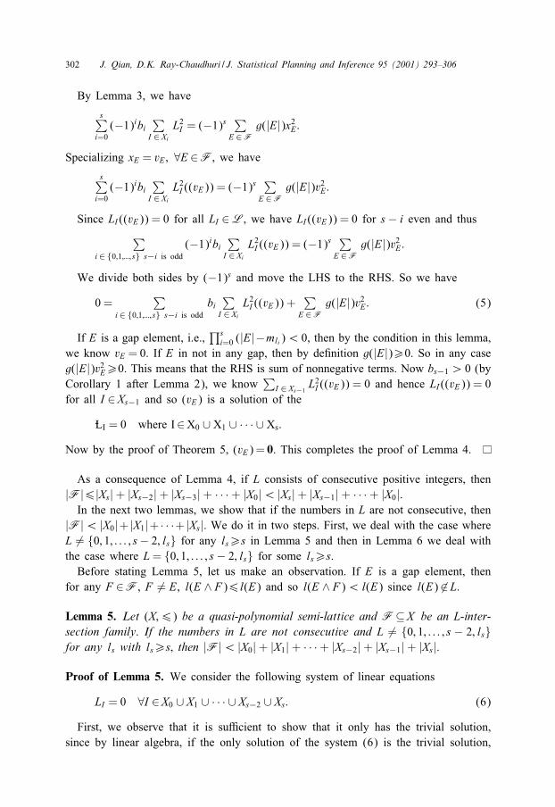
Lemma 4. Let (X;6) be a quasi-polynomial semi-lattice of height n; L={l1; : : : ; ls};s∈N. Suppose (vE)E ∈F is a solution of system of linear equations: LI = 0 for allI ∈Xs ∪ Xs−2 ∪ Xs−3 ∪ Xs−4 ∪ · · · ∪ X0. If vE = 0 for all gap element E ∈F, thenvE = 0 for all E ∈F.

Proof. Suppose W0 contains (vE). It suAces to show vE = (0; 0; : : : ; 0).


By Lemma 3, we have

s∑i=0(−1)ibi

∑I ∈ Xi

L2I = (−1)s∑E ∈F

g(|E|)x2E:

Specializing xE = vE; ∀E ∈F, we have

s∑i=0(−1)ibi

∑I ∈ Xi

L2I ((vE)) = (−1)s∑E ∈F

g(|E|)v2E:

Since LI ((vE)) = 0 for all LI ∈L, we have LI ((vE)) = 0 for s− i even and thus∑

i∈{0;1;:::; s} s−i is odd(−1)ibi

∑I ∈ Xi

L2I ((vE)) = (−1)s∑E ∈F

g(|E|)v2E:

We divide both sides by (−1)s and move the LHS to the RHS. So we have0 =

∑i∈{0;1;:::; s} s−i is odd

bi∑I ∈ Xi

L2I ((vE)) +∑E ∈F

g(|E|)v2E: (5)

If E is a gap element, i.e.,∏si=0 (|E|−mli)¡ 0, then by the condition in this lemma,

we know vE = 0. If E in not in any gap, then by de4nition g(|E|)¿0. So in any caseg(|E|)v2E¿0. This means that the RHS is sum of nonnegative terms. Now bs−1¿ 0 (byCorollary 1 after Lemma 2), we know

∑I ∈ Xs−1 L

2I ((vE)) = 0 and hence LI ((vE)) = 0

for all I ∈Xs−1 and so (vE) is a solution of the-LI = 0 where I∈X0 ∪ X1 ∪ · · · ∪ Xs:

Now by the proof of Theorem 5, (vE) = 0. This completes the proof of Lemma 4.

As a consequence of Lemma 4, if L consists of consecutive positive integers, then|F|6|Xs|+ |Xs−2|+ |Xs−3|+ · · ·+ |X0|¡ |Xs|+ |Xs−1|+ · · ·+ |X0|.In the next two lemmas, we show that if the numbers in L are not consecutive, then

|F|¡ |X0|+ |X1|+ · · ·+ |Xs|. We do it in two steps. First, we deal with the case whereL �= {0; 1; : : : ; s− 2; ls} for any ls¿s in Lemma 5 and then in Lemma 6 we deal withthe case where L= {0; 1; : : : ; s− 2; ls} for some ls¿s.Before stating Lemma 5, let us make an observation. If E is a gap element, then

for any F ∈F, F �= E, l(E ∧ F)6l(E) and so l(E ∧ F)¡l(E) since l(E) �∈L.

Lemma 5. Let (X;6) be a quasi-polynomial semi-lattice and F⊆X be an L-inter-section family. If the numbers in L are not consecutive and L �= {0; 1; : : : ; s − 2; ls}for any ls with ls¿s; then |F|¡ |X0|+ |X1|+ · · ·+ |Xs−2|+ |Xs−1|+ |Xs|.

Proof of Lemma 5. We consider the following system of linear equations

LI = 0 ∀I ∈X0 ∪ X1 ∪ · · · ∪ Xs−2 ∪ Xs: (6)

First, we observe that it is suAcient to show that it only has the trivial solution,since by linear algebra, if the only solution of the system (6) is the trivial solution,


then

|F| = the number of variables6 the number of equations

= |X0|+ |X1|+ · · ·+ |Xs−2|+ |Xs|:Suppose (vE)E ∈F is a solution. We hope to show (vE) is the all 0 vector in R|F|.

By Lemma 4, it is suAcient to prove that vE = 0 for every gap element E ∈F, i.e.,vE=0 for all E ∈F for which there exists i∈{1; 2; : : : ; s−1} with li ¡ l(E)¡li+1. We4x such a gap element E. Note that since li¿i − 1, we have l(E)¿i. We distinguishtwo cases.Case 1: l(E)¿i + 1.Since i6s− 1, we have two subcases:Case 1.1: i= s− 1. In this situation, we have l(E)¿i+ 1= s and so there are two

possibilities for E.Case 1.1.1: l(E)= s. In this subcase, E ∈Xs and so LE =0. Note that if there exists

an F ∈F with E¡F , then l(F ∧E)= l(E) �∈L, a contradiction. So we have LE = xE .By specializing (xF)F ∈F = (vF)F ∈F in LE = 0, we have vE = 0.Case 1.1.2: l(E)¿s. Since {l1; l2; : : : ; ls−1; l(E)} �= {0; 1; : : : ; s − 1}, by Lemma 1

we have

A:=

f0(ml1 ) f1(ml1 ) · · · fs−2(ml1 ) fs(ml1 )· · · · · · · · · · · · · · ·

f0(mls−1 ) f1(mls−1 ) · · · fs−2(mls−1 ) fs(mls−1 )f0(|E|) f1(|E|) · · · fs−2(|E|) fs(|E|)

is non-singular.So there exists

a =

a0a1...as−1

such that

Aa =

00...01

: (7)

As before, �I (E) is de4ned to be 1 if I6E and 0 otherwise. We have

s−2∑j=0aj

∑I ∈ Xj

LI �I (E) + as−1∑I ∈ Xs

LI�I (E) = xE: (8)


In fact, on the left-hand side of the above equation, the coeAcient of xF is

s−2∑j=0ajfj(|F ∧ E|) + as−1fs(|E ∧ F |): (9)

By the observation before Lemma 5, if F �= E, then l(F ∧ E)¡l(E) and l(F ∧E)∈{l1; l2; : : : ; ls−1}, and so (7) implies that (9)=0, which proves the above equation.This proves (8).If we specialize xF = vF for all F ∈F, the left-hand side of (8) will be 0, from

which we get vE = 0.Case 1.2: i6s− 2.Let f(x) = (x − ml1 )(x − ml2 ) · · · (x − mli), then there exist a0; a1; : : : ; ai ∈Q such

that∑ij=0 ajfj(x) = f(x). Notice that if F �= E, then l(F ∧ E)6l(E), hence l(F ∧

E)∈{l1; l2; : : : ; li} and f(|E ∧ F |) = 0. We havei∑j=0aj

∑I ∈ Xj

LI �I (E) =∑F ∈F

f(|E ∧ F |)xF :

=f(|E ∧ E|)xE=f(|E|)xE: (10)

Now, if we specialize that (xF)F ∈F=(vF)F ∈F, both the left- and the right-hand sideof (10) are equal to 0. So again vE = 0 since f(|E|) �= 0.Case 2: l(E) = i.In this case, we have {l1; l2; : : : ; li}= {0; 1; : : : ; i− 1}. If i= s− 1, then l1 = 0; l2 =

1; : : : ; ls−1 = s− 2, and so {l1; l2; : : : ; ls}= {0; 1; : : : ; s− 2; ls}, which is a contradictionto our hypothesis. So i6s− 2 and therefore E ∈X0 ∪X1 ∪ · · · ∪Xs−2 ∪Xs. This impliesLE is one of the equations in (6) and so LE((vF)) = 0. Further, we get that LE = xEby the same argument as in the proof (8). So we have vE = 0.

Lemma 6. Let (X;6) be a quasi-polynomial semi-lattice and F⊆X be an L-inter-section family. If L={0; 1; : : : ; s−2; ls}, where ls¿s; then |F|¡ |X0|+|X1|+· · ·+|Xs|.

Proof. Again we have two cases.

Case 1: Xs−1⊆F.It is clear that F does not contain an element E with l(E)¿s (otherwise s − 1

would be an intersection size, which contradicts to the condition in Lemma 6). So|F|6|X0|+ |X1|+ · · ·+ |Xs−1|, which proves Lemma 6.Case 2: Xs−1 *F.In this case, |F∩Xs−1|¡ |Xs−1|. We want to show that the system of linear equations

{LI = 0 ∀I ∈X0 ∪ X1 ∪ · · · ∪ Xs−2 ∪ Xs;xI = 0 ∀I ∈F; l(I) = s− 1 (11)


has only trivial solution, which will show that

|F|6 |X0|+ |X1|+ · · ·+ |Xs−2|+ |Xs|+ |F ∩ Xs−1|¡ |X0|+ |X1|+ · · ·+ |Xs−2|+ |Xs−1|+ |Xs|:

Suppose (11) has a solution (vE)E ∈F, we want to show it is equal to 0. By Lemma4, we only need to show that vE = 0 for any E ∈F with s− 2¡l(E)¡ls. Note thatl(E)¿s− 1, we distinguish two subcases.Case 2.1: l(E) = s − 1, in this case it is obvious that vE = 0 since (vE) satis4esxE = 0;Case 2.2: l(E)¿s, let I be such that I6E and I ∈Xs. Note that if E ∈Xs, we can

take I to be E. We contend that LI=xE . Since otherwise there exists F ∈F with F �= Eand I6F . This implies that I6F ∧E and l(F ∧E)¿s which forces l(F ∧E)= ls, butthis is a contradiction because l(E)¡ls.

Lemma 7. Let (X;6) be a quasi-polynomial semi-lattice. If F is an L-intersectionfamily for L = {0; 1; : : : ; s − 1}; then |F| = |X0| + |X1| + · · · + |Xs| if and only ifF= X0 ∪ X1 ∪ · · · ∪ Xs.

Proof. Let l = |⋃si=0 Xi| =∑si=0 |Xi|. We consider the |F| by l incidence matrix M

whose rows are indexed by elements of F and whose columns are indexed by elementsof Ys, where Ys:=

⋃si=0 Xi. For A∈F; S ∈Ys, the (A; S)-entry of M is de4ned to be

1 if either A∈Ys and S = A or A∈X − Ys; S ∈Xs and S6A. It is de4ned to be 0otherwise.Observations: It is clear from the above de4nition of M that

(1) if (A; S)-entry of M is 1 then S6A,(2) each row has at least one non-zero entry and(3) if A∈F and A∈Xu; u¿ s, then the row corresponding to A has fs(mu)¿ 1non-zero entries (see the de4nition of quasi polynomial semilattice).

Claim. For A �= B∈F; the (A; B)-entry in MMT is 0.

Proof. Suppose (A; B)-entry of MMT is ¿1. Then there exists an S ∈Ys such that both(A; S)-entry and (B; S)-entry of M are 1. By observation (1), S6A∧B, so S ∈ ⋃s−1

i=0 Xi=Ys−1 since F is a {0; 1; : : : ; s − 1}-intersection family. But from the de4nition of M ,for such an S, (A; S)-entry of M is 1 if and only if A = S. The same is true for the(B; S)-entry. So A= S = B, which is a contradiction. This proves the claim.From the above claim, it is clear that MMT is a diagonal matrix, and it is also

clear that the diagonal entries are non-zero by observation (2) above. So MMT is anon-singular |F| by |F| matrix.Now suppose |F|=∑s

i=0 |Xi|, so M is a square matrix. It is clear that each columnof M can contain at most one non-zero entry, otherwise MMT would not be a diagonalmatrix. So the total number of 1’s in M is 6|F|. Therefore, by observation (2) thetotal number of 1’s in M is |F|. So each row of M should contain exactly one


non-zero entry by the above observations. This means that A∈Ys for any A∈F. SoF⊆Ys =

⋃si=0 Xi. But |F|=∑s

i=0 |Xi|, so F=⋃si=0 Xi.

Proof of Theorem 6. Let F be an L-intersection family and |F| = {0; 1; : : : ; s − 1},then by Lemma 7 the proof is complete. In the following, we show that if L �={0; 1; : : : ; s − 1} then |F|¡ |X0| + |X1| + · · · + |Xs|, which would 4nish the proof ofTheorem 6. We distinguish two cases.Case 1: L is not consecutive.In this case, if L={0; 1; : : : ; s−2; ls} for some integer ls¿s, Lemma 6 completes the

proof. If L is not of the form {0; 1; : : : ; s− 2; ls} for some ls¿s, Lemma 6 completesthe proof.Case 2: L is consecutive but not equal to {0; 1; : : : ; s− 1}.In this case, there is no gap element E ∈F and therefore by Lemma 4 we know

that the system of linear equations: LI = 0 for all I ∈Xs ∪ Xs−2 ∪ Xs−4 ∪ · · · ∪ Xs−2[s=2]has only trivial solution. From this, we deduce that the number of variables is lessthan or equal to the number of equations, i.e.,

|F|6 |Xs|+ |Xs−2|+ |Xs−4|+ · · ·+ |Xs−2[s=2]|¡ |Xs|+ |Xs−1|+ |Xs−1|+ · · ·+ |X0|

which completes the proof of Theorem 6.

References

Alon, N., Babai, L., Suzuki, H., 1991. Multilinear polynomials and Frankl–Ray-Chaudhuri–Wilson typeintersection and theorems. J. Combin. Theory A 58, 165–180.

Bose, R.C., 1949. A note on Fisher’s inequality for balanced incomplete block design. Ann. Math. Stat. 20,619–620.

de Bruijn, N.G., Erd=os, P., 1948. On a combinatorial problem. Proc. Kon. Ned. Akad. v. Wetensch 51,1277–1279.

Frankl, P., Wilson, R.M., 1981. Intersection theorem with geometric consequences. Combinatorica 1 (4),357–368.

Qian, J., Ray-Chaudhuri, D.K., 1997. Frankl–F=uredi Type inequalities for polynomial semi-lattices. Elec. J.Combin. 4, 28.

Qian, J., Ray-Chaudhuri, D.K., 2001. Combinatorial inequalities on quasi-polynomial semi-lattices, submittedfor publication.

Ramanan, G.V., 2001. Proof of a conjecture of Frankl and F=uredi, J. Combin. Theory A, to appear.Ray-Chaudhuri, D.K., Tianbao Zhu, 1993. S-intersection families and tight designs. Coding Theory, DesignTheory, Group Theory, Proceeding of Marshall Hall Conference. Wiley, New York, pp. 67–75.

Ray-Chaudhuri, D.K., Wilson, R.M., 1975. on t-designs. Osaka J. Math. 12, 737–744.

extremal case of frankl–ray-chaudhuri–wilson inequality

Documents