Extreme Events, Heavy Tails, and the Generating Processes:

Examples from Hydrology and Geomorphology

Efi Foufoula-Georgiou

SAFL, NCED

University of Minnesota

E2C2 – GIACS Advanced School on “Extreme Events: Nonlinear Dynamics and Time Series Analysis

Comorova, Romania

September 3-11, 2007

In Hydrology and Geomorphology “Fluctuations” around the mean behavior are of high magnitude.

Understanding their statistical behavior is useful for prediction of extremes and also for understanding spatio-temporal heterogeneities which are hallmarks of the underlying process- generating mechanism.

These fluctuations are often found to exhibit power law tails and scaling

Underlying Theme

PRESENCE OF SCALING

... scaling laws never appear by accident. They always manifest a property of the phenomenon of basic importance … This behavior should be discovered, if it exists, and its absence should also be recognized.”

Barenblatt (2003)

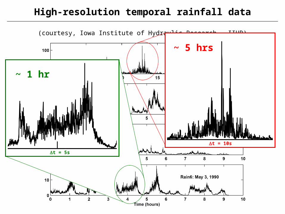
High-resolution temporal rainfall data

(courtesy, Iowa Institute of Hydraulic Research – IIHR)

~ 5 hrs

t = 10s

~ 1 hr

t = 5s

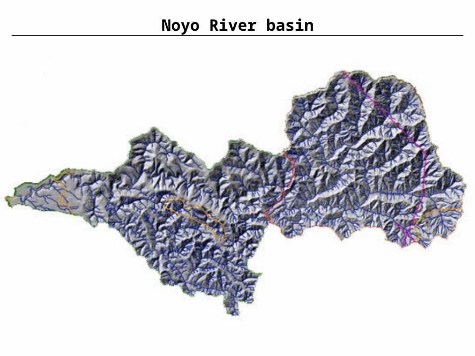
Noyo River basin

STREAMLAB 2006

Data Available:

-Sediment accumulation series

-Time series of bed elevation

-Laser transects of bed elevation

Pan-1 Pan-2 Pan-3 Pan-4 Pan-5

Bed Elevation

0 100 200 300 400 5000

100

200

300

h(t)

(m

m)

Q = 4300 lps

0 100 200 300 400 5000

100

200

300

time (min)

h(t)

(m

m)

Q = 5500 lps

= 28.64 mm = 9.79 mm

= 184.14 mm = 65.78 mm

Noise-free sediment transport rates

Weigh pan bedload transport rates (Q = 5.5 m3/s) (a) 1 s averaging and 0 point skip (b) 15s averaging time and 6 point skip (from Ramooz and Rennie, 2007)

• Characterize a signal f(x) in terms of its local singularities

( ) ( ) ( )0

0 0

h xf x f x Ce e- + £ ×

Ex: h(x0) = 0.3 implies f(x) is very rough around x0.

h(x0) = 0.7 implies a “smoother” function around xo.

Localized Scaling Analysis: Multifractal Formalism

h=0.3

h=0.7

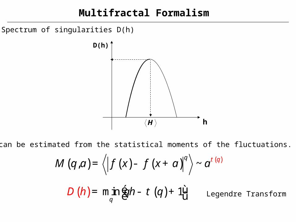
• Spectrum of singularities D(h)

• D(h) can be estimated from the statistical moments of the fluctuations.

( ) ( ) ( ) ( ), ~ qqM q a f x f x a a t= - +

( ) ( )min 1qqh h qD té ù= - +ë û Legendre Transform

Multifractal Formalism

h

D(h)

H

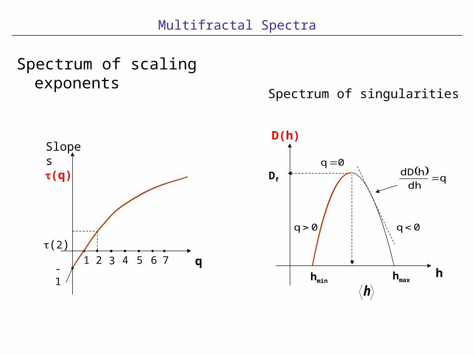
Multifractal Spectra

• Spectrum of scaling exponents (q) and Spectrum of singlularities D(h)

monofractal

multifractal

h

h

1

2 0

c H

c

=

=

1

2 0

c

c ¹

Multifractal Spectra

Spectrum of scaling exponents

h

Spectrum of singularities

-11 2 3 4 5 6 7

(2)

Slopes (q)

q

D(h)

0q

0q 0q

q

dh

hdDDf

hmin hmax

h

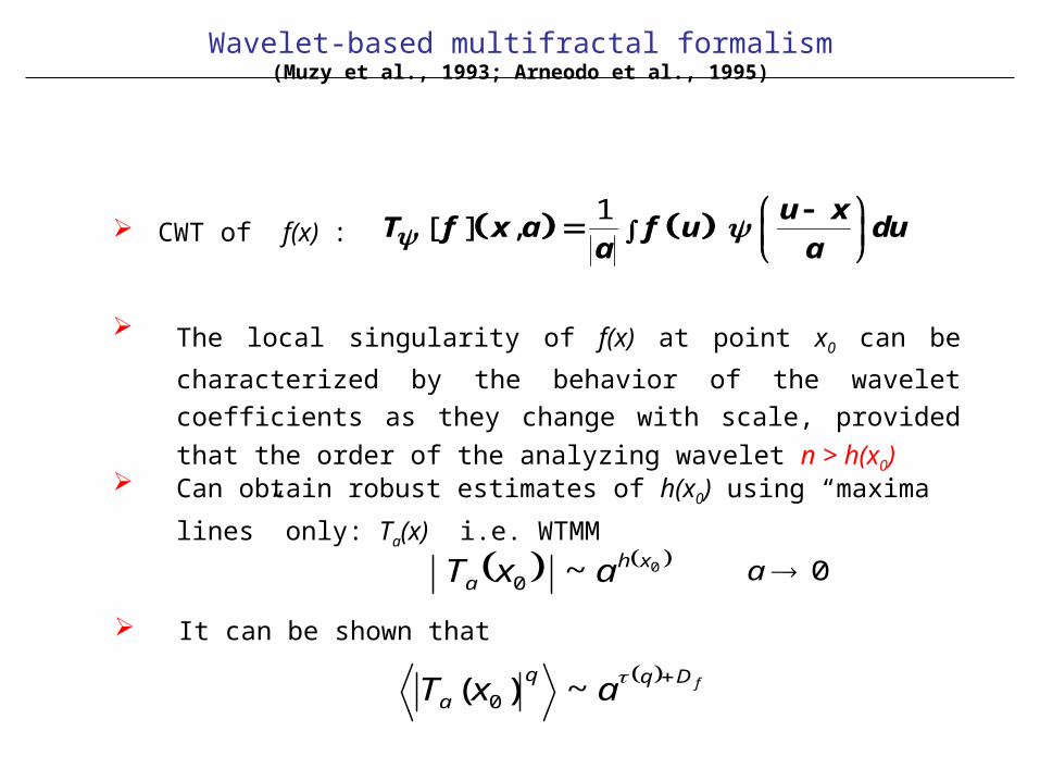
Wavelet-based multifractal formalism(Muzy et al., 1993; Arneodo et al., 1995)

1[ ] ,

u xT f x a f u du

a a

CWT of f(x) :

The local singularity of f(x) at point x0 can be characterized

by the behavior of the wavelet coefficients as they change with scale, provided that the order of the analyzing wavelet

n > h(x0)

Can obtain robust estimates of h(x0) using “maxima lines”

only: Ta(x) i.e. WTMM

0~ 0xh

a axT 0a

It can be shown that

fDqq

a axT ~)( 0

f(x)

T[f](x,a)

WTMMTa(x)

Structure FunctionMoments of

|f(x+l) – f(x)|

Partition FunctionMoments of|T[f](x,a)|

Partition FunctionMoments of |Ta(x)| (access to q < 0)

Cumulant analysisMoments of ln |Ta(x)|

(direct access to statistics of singularities)

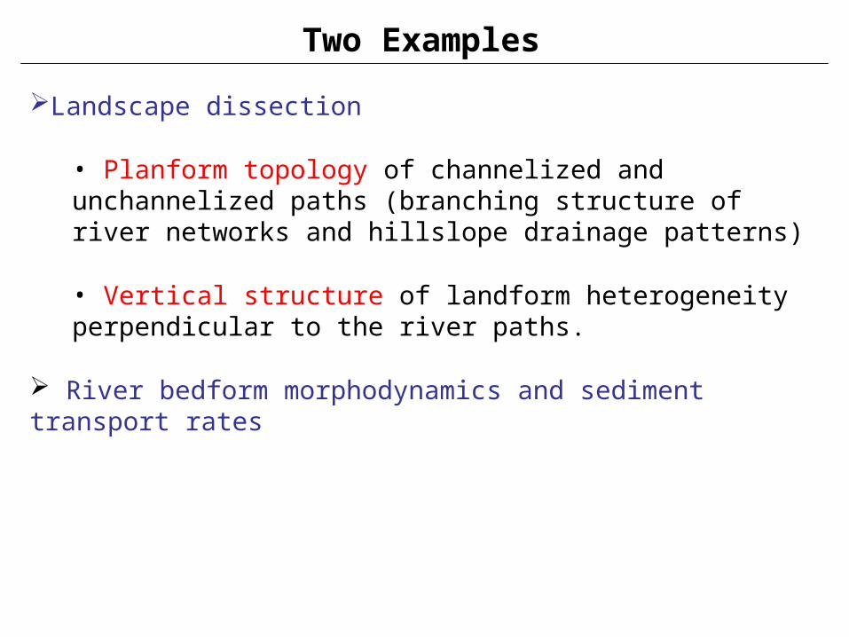
Landscape dissection

• Planform topology of channelized and unchannelized paths (branching structure of river networks and hillslope drainage patterns)

• Vertical structure of landform heterogeneity perpendicular to the river paths.

River bedform morphodynamics and sediment transport rates

Two Examples

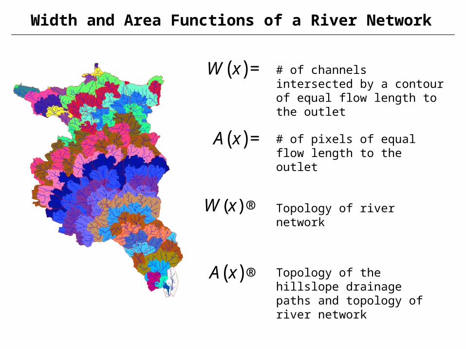
Width and Area Functions of a River Network

( )W x =

( )A x =

( )W x ®

( )A x ®

# of channels intersected by a contour of equal flow length to the outlet

# of pixels of equal flow length to the outlet

Topology of river network

Topology of the hillslope drainage paths and topology of river network

Width and Area Functions of a River Network

( )W x =

( )A x =

( )W x ®

( )A x ®

# of channels intersected by a contour of equal flow length to the outlet

# of pixels of equal flow length to the outlet

Topology of river network

Topology of the hillslope drainage paths and topology of river network

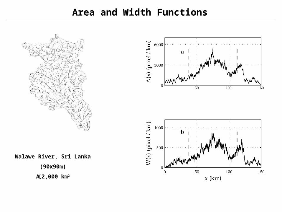
Area and Width Functions

Walawe River, Sri Lanka

(90x90m)

A2,000 km2

Area and Width Functions

Noyo River Basin, California, USA

(10x10m)

A143 km2

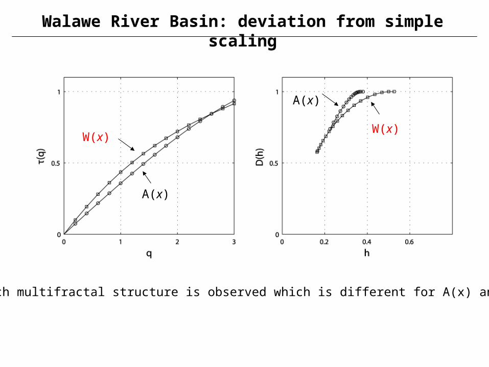
Walawe River Basin: deviation from simple scaling

A rich multifractal structure is observed which is different for A(x) and W(x)

A(x)

A(x)

W(x)W(x)

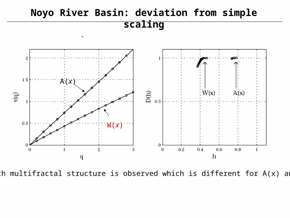
Noyo River Basin: deviation from simple scaling

A rich multifractal structure is observed which is different for A(x) and W(x)

A(x)

W(x)

Noyo River Basin (10x10m; A143 km2)

c1 0.77 c2 0.11 SR = 0.07 - 0.43 km

-“Hillslope” path dominated

-“smoother” overall than W(x)

-Hillslope drainage dissection is s-s between scales 0.1 km – 0.5km

-Statistics of the density of hillslope drainage paths strongly depend on scale

c1 0.46 c2 0.10 SR = 0.13 – 0.70 km

-River network path dominated

-“Rougher “overall” than A(x)

-Channel network landscape dissection is s-s between scales 0.1 km to 0.7 km

-Strong inntermittency (higher moments of pdf of channel drainage density has a strong dependence on scale)

Pay attention not only to the average properties of landscape dissection but to higher moments

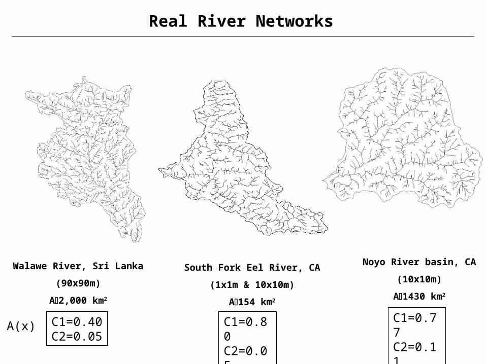
Real River Networks

Walawe River, Sri Lanka

(90x90m)

A2,000 km2

South Fork Eel River, CA

(1x1m & 10x10m)

A154 km2

Noyo River basin, CA

(10x10m)

A1430 km2

C1=0.40C2=0.05

C1=0.80C2=0.05

C1=0.77C2=0.11A(x)

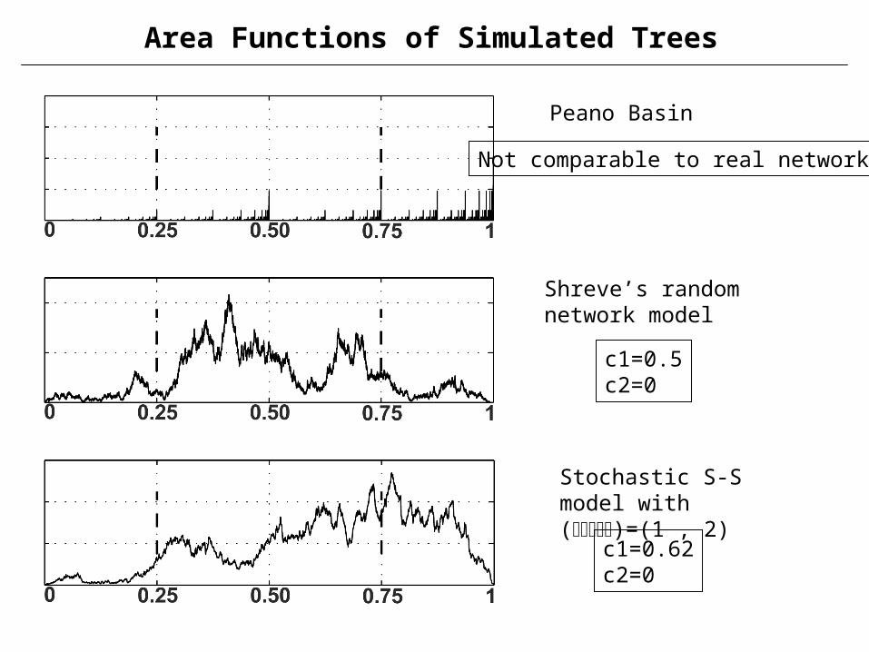
Area Functions of Simulated Trees

Peano Basin

Shreve’s randomnetwork model

Stochastic S-S model with ()=(1 , 2)

c1=0.5c2=0

c1=0.62c2=0

Not comparable to real networks

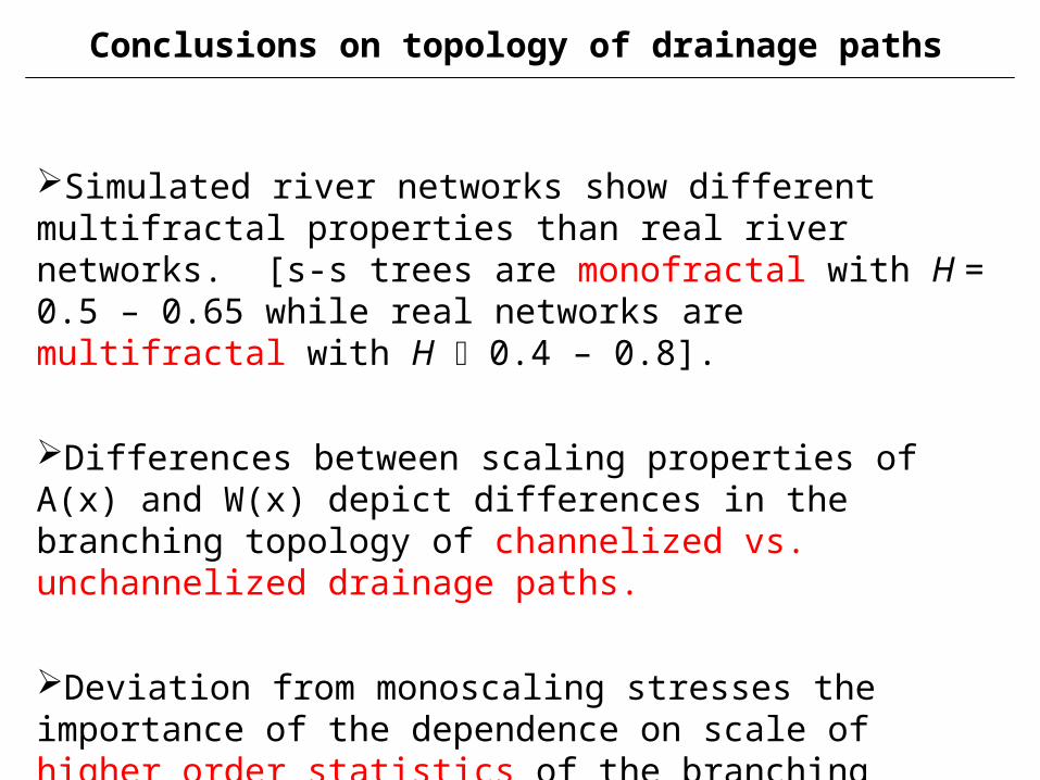
Conclusions on topology of drainage paths

Simulated river networks show different multifractal properties than real river networks. [s-s trees are monofractal with H = 0.5 – 0.65 while real networks are multifractal with H 0.4 – 0.8].

Differences between scaling properties of A(x) and W(x) depict differences in the branching topology of channelized vs. unchannelized drainage paths.

Deviation from monoscaling stresses the importance of the dependence on scale of higher order statistics of the branching structure.

Implications for Network Hydrology?

Conjecture: Deviation from scale invariance in W(x), implies that the variability of the in-phase hillslope hydrographs entering the network depends on “scale”

Implications for routing? scale-dependent convolution? geomorphologic dispersion?

Implications for scaling of hydrographs?

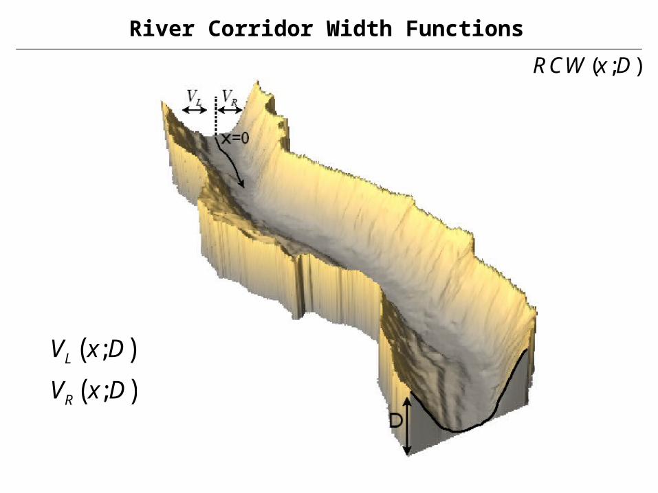
River Corridor Width Functions

( )( )

;

;

L

R

V x D

V x D

( ; )RCW x D

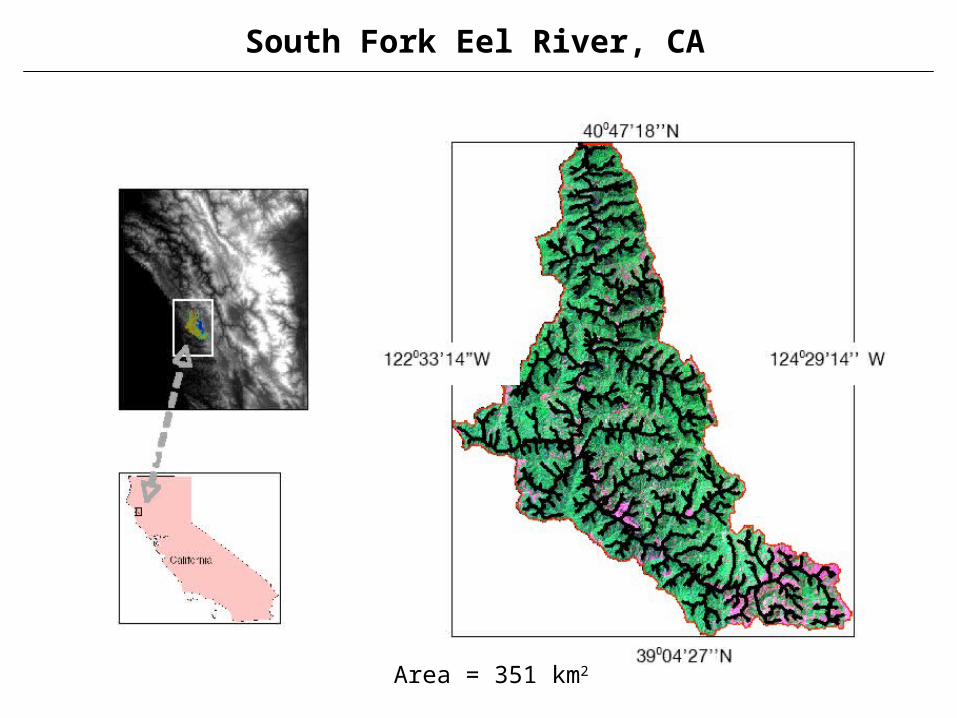
Area = 351 km2

South Fork Eel River, CA

River Corridor Width Function (D=5m)

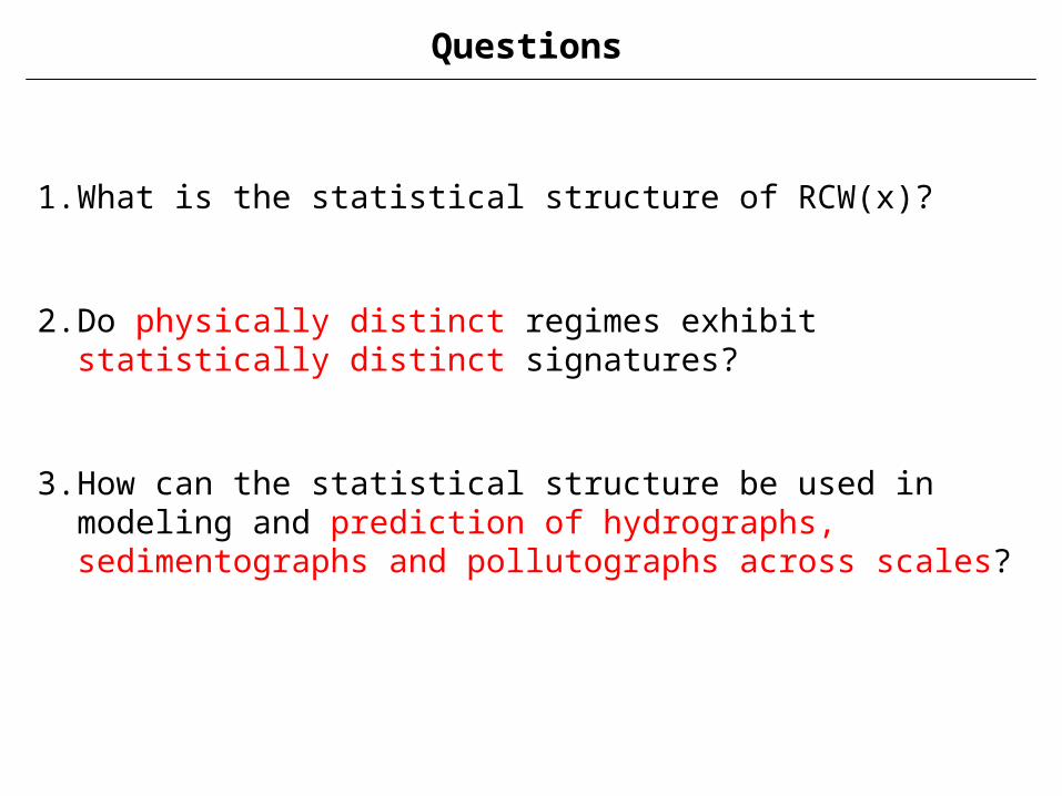
1. What is the statistical structure of RCW(x)?

2. Do physically distinct regimes exhibit statistically distinct signatures?

3. How can the statistical structure be used in modeling and prediction of hydrographs, sedimentographs and pollutographs across scales?

Questions

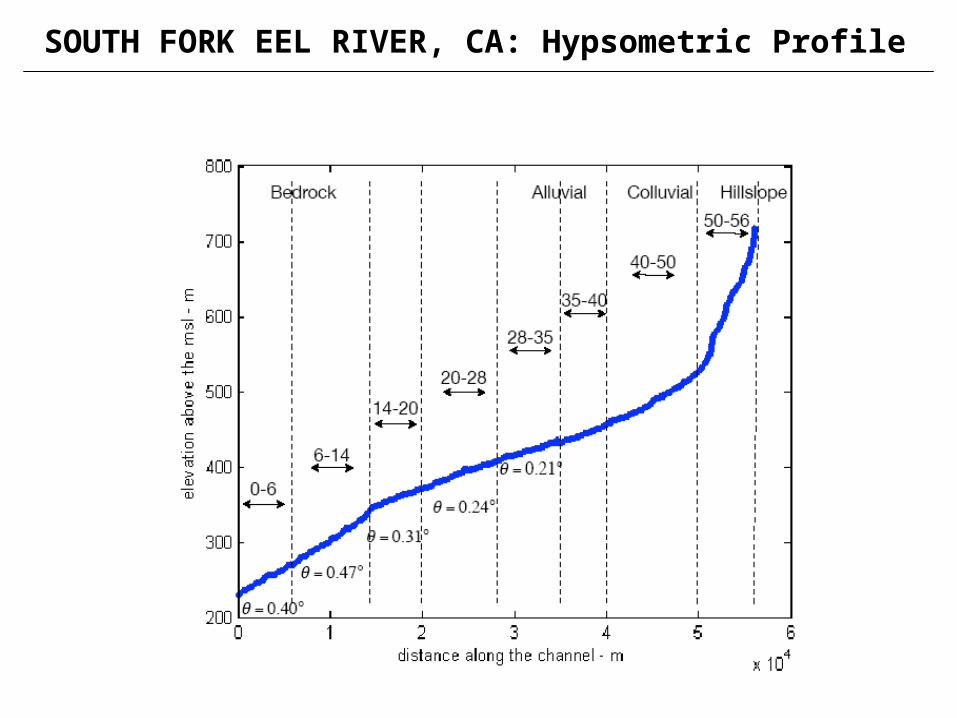
SOUTH FORK EEL RIVER, CA: Hypsometric Profile

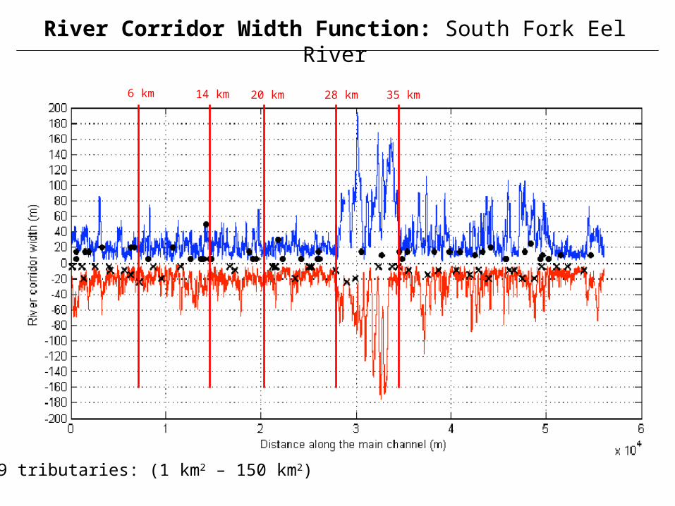
89 tributaries: (1 km2 – 150 km2)

River Corridor Width Function: South Fork Eel River

6 km 14 km 20 km 28 km 35 km

River Reach: 0-6 km

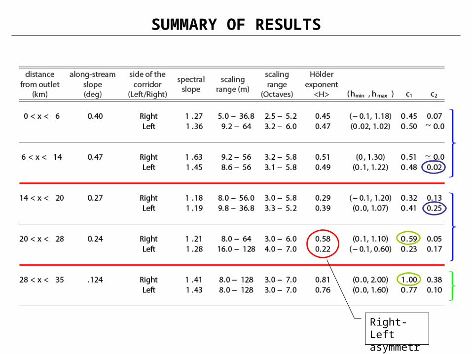
SUMMARY OF RESULTS

Right-Left asymmetry

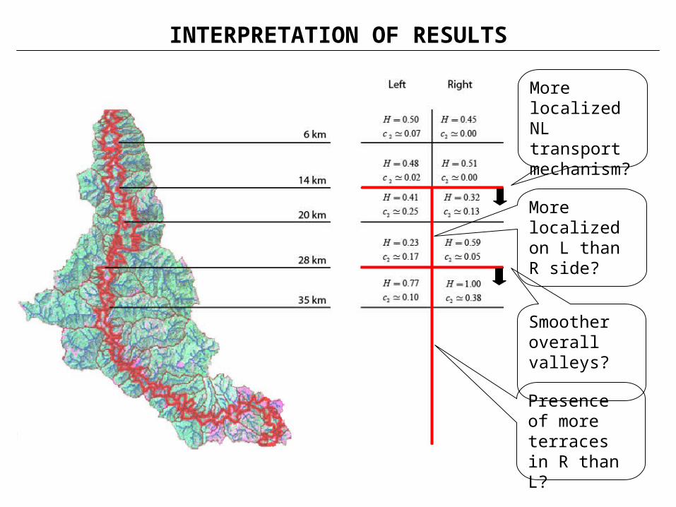
INTERPRETATION OF RESULTS

More localized NL transport mechanism?

More localized on L than R side?

Smoother overall valleys?

Presence of more terraces in R than L?

Conclusions and Open Questions…

• Hillslope “roughness” seems to carry the signature of valley forming processes; need to provide a complete hierarchical characterization. Do hillslope evolution models reproduce this structure? What is the effect on hillslope sediment variability of the higher order statistics of travel paths to streams?

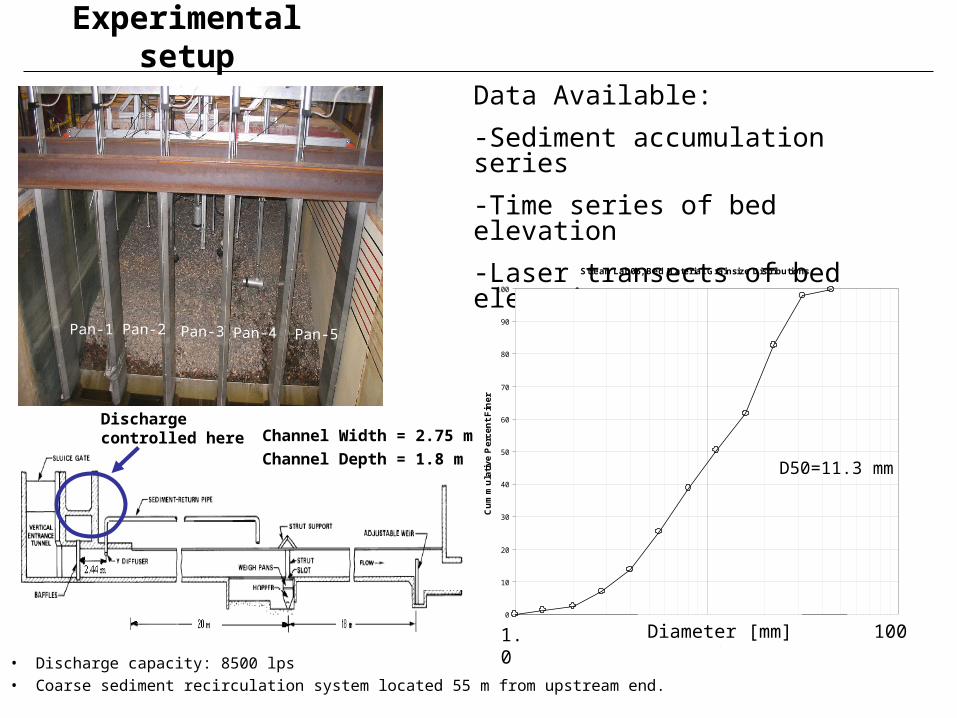
Experimental setup

Data Available:

-Sediment accumulation series

-Time series of bed elevation

-Laser transects of bed elevation

Pan-1 Pan-2 Pan-3 Pan-4 Pan-5D50 = 11.3mm

StreamLab06, Bed Material Grainsize Distributions

0

10

20

30

40

50

60

70

80

90

100

1.0 10.0 100.0

diameter (mm)

Cu

mm

ula

tiv

e P

erc

en

t F

ine

r

1.0 100Diameter [mm]

Discharge controlled here Channel Width = 2.75 m

Channel Depth = 1.8 m

• Discharge capacity: 8500 lps• Coarse sediment recirculation system located 55 m from upstream end.

D50=11.3 mm

QUESTIONS

1. Do the statistics of sediment transport rates depend on “scale” (sampling interval or time interval of averaging) and how?

2. Does this statistical scale-dependence depend on flow rate, bed shear stress, and bedload size distribution (e.g., gravel vs. sand, etc.)

3. Do the statistics of sediment transport relate to the statistics of bedform morphodynamics and how?

4. What are the practical implications of all these?

0 5 10

x 104

0

100

200

300Q=4300 lps

time(sec)

Sc(t

) kg

)

0 5 10

x 104

-1

0

1 Q=4300 lps

time(sec)

S(t

)(kg

)0 5 10

x 104

0

5000 Q=4900lps

time(sec)

Sc(t

)(kg

)

0 5 10

x 104

-2

0

2 Q=4900 lps

time(sec)S

(t)(

kg)

0 5 10

x 104

0

1

2

3x 10

4

Q=5500 lps

time(sec)

Sc(t

)(kg

)

0 5 10

x 104

-5

0

5 Q=5500 lps

time(sec)

S(t

)(kg

)

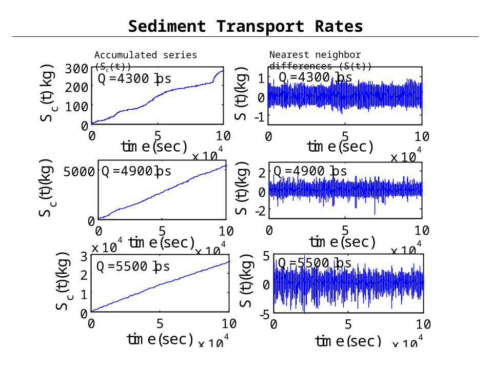
Sediment Transport Rates

Accumulated series (Sc(t)) Nearest neighbor differences (S(t))

0 2 4 6 8 10

x 104

0

0.5

1

1.5

2

2.5

3x 10

4

Q=5500 lps

time(sec)

Sc(t

)(kg

)

0 20 40 60 80 100 1201.2736

1.2738

1.274

1.2742

1.2744

1.2746

1.2748

1.275x 10

4

Q=5500 lps

time(sec)

Sc(t

)(kg

)

0 200 400 600 800 1000 12001.265

1.27

1.275

1.28

1.285

1.29

1.295

1.3

1.305x 10

4 Q=5500 lps

time(sec)

Sc(t

)(kg

)

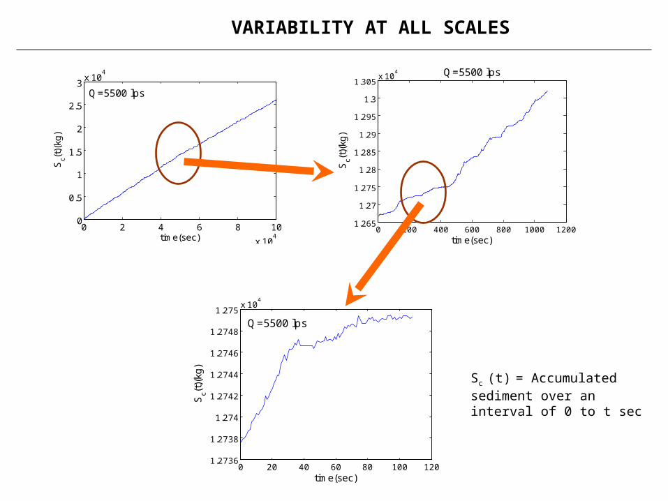
VARIABILITY AT ALL SCALES

Sc (t) = Accumulated sediment over an interval of 0 to t sec

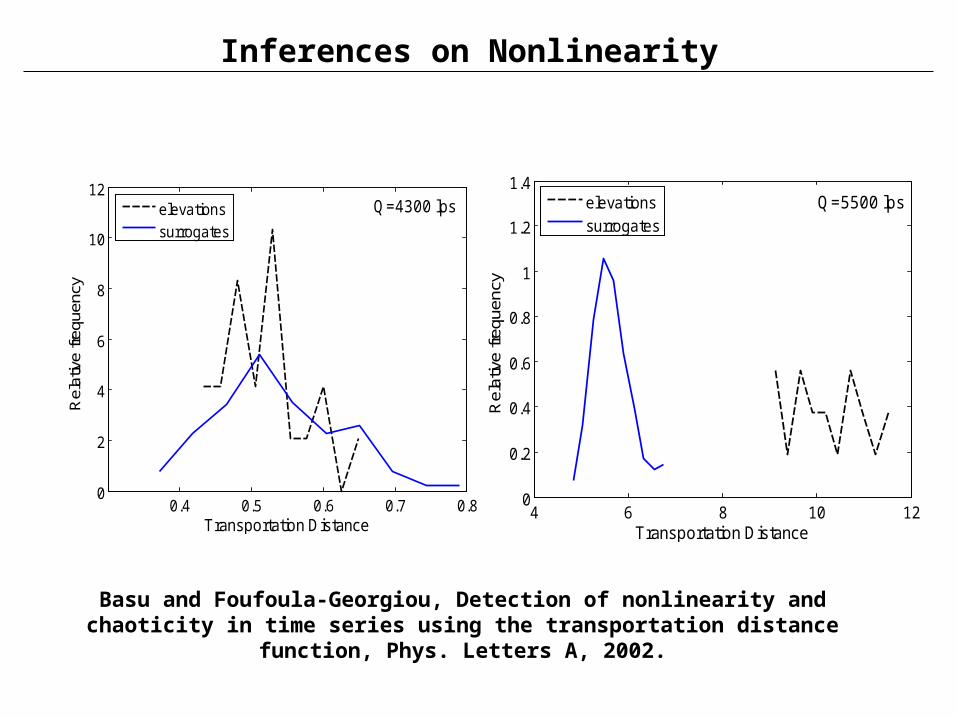
ANALYSIS METHODOLOGY: ADVANTAGES

1. Local analysis (as opposed to global, e.g., spectral analysis)

2. Can characterize the statistical structure of localized abrupt fluctuations over a range of scales

3. Wavelet-based multifractal formalism -- uses generalized fluctuations instead of standard differences (f(x) – f(x+dx))

Can automatically remove non-stationarities in the signal both in terms of overall trends and in terms of low-frequency oscillations coming from dune or ripple effects

Can automatically remove noise in the signals and point to the minimum scale that can be safely interpreted

Can characterize effectively how pdfs change with scale with only one or two parameters

Noise Variability levels off

1 min 15 min

4 6 8 10 12 140

5

10

15

20

25

30

35

40

45Q = 5500 lps

log2(a) (sec)

S(q

,a)

q = 0.5

q = 1.0

q = 1.5

q = 2.0

q = 2.5

q = 3.0

Scaling range

0 1 2 3 40

0.5

1

1.5

2

2.5

3

3.5

4

(q

)

Q = 5500 lps

q

SEDIMENT TRANSPORT RATES: Q = 5500 lpslo

g 2

C1=1.10C2=0.10

Noise Statistical Variability regime changes

1 min 10 min

Scaling range

0 0.5 1 1.5 2 2.5 3 3.50

0.5

1

1.5

2

2.5

3

3.5

4

(q)

Q=4300 lps

q4 6 8 10 12 14

0

5

10

15

20

25

30

35

40

45Q = 4300 lps

log2(a) (sec)

S(q

,a)

q =3.0

q =2.5

q =2.0

q =1.5

q =1.0

q =0.5

Q = 4300 lpslo

g 2

C1=0.55C2=0.15

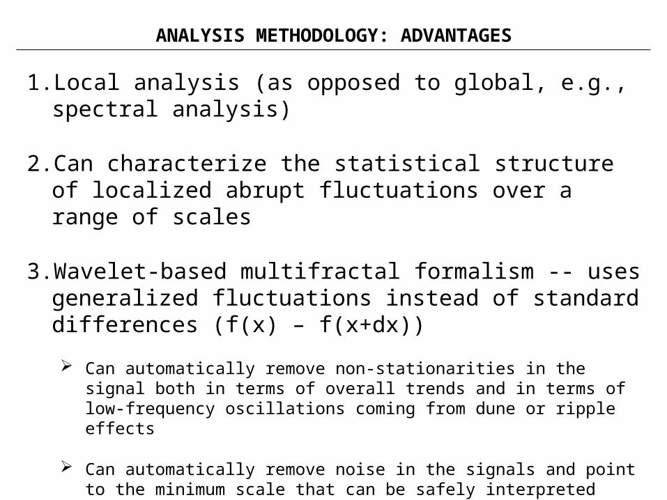
Bed Elevation

0 100 200 300 400 5000

100

200

300

h(t)

(m

m)

Q = 4300 lps

0 100 200 300 400 5000

100

200

300

time (min)

h(t)

(m

m)

Q = 5500 lps

= 28.64 mm = 9.79 mm

= 184.14 mm = 65.78 mm

BED ELEVATION TEMPORAL SERIES: Q = 5500 lps

0 1 2 3 40

0.5

1

1.5

2

2.5

3

3.5

4

(q)

Q = 5500 lps

q1 2 3 4 5 6 7 8

0

5

10

15

20

25

30

35

40

45Q = 5500 lps

log2(a) (sec)

log

2 S

(q,a

)

q = 3.0

q = 2.5

q = 2.0

q = 1.5

q = 1.0

q = 0.5

Scaling range

0.5 min 8 min C1=0.70C2=0.11

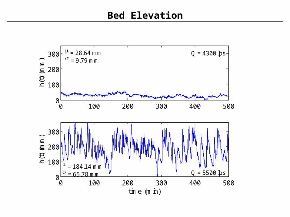
BED ELEVATION TEMPORAL SERIES: Q = 4300 lps

0 1 2 3 40

0.5

1

1.5

2

2.5

3

3.5

4

(q)

Q = 4300 lps

q2 3 4 5 6 7 8

5

10

15

20

25

30

35

40

45Q = 4300 lps

log2(a) (sec)

log

2 S

(q,a

)

q = 3.0

q = 2.5

q = 2.0

q = 1.5

q = 1.0

q = 0.5

Scaling range

12 min1 min C1=0.55C2=0.05

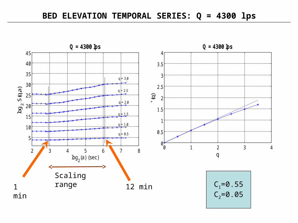
Inferences on Nonlinearity

0.4 0.5 0.6 0.7 0.80

2

4

6

8

10

12Q=4300 lps

Rel

ativ

e fre

quen

cy

Transportation Distance

elevationssurrogates

4 6 8 10 120

0.2

0.4

0.6

0.8

1

1.2

1.4Q=5500 lps

Rel

ativ

e fre

quen

cy

Transportation Distance

elevationssurrogates

Basu and Foufoula-Georgiou, Detection of nonlinearity and chaoticity in time series using the transportation distance function, Phys. Letters A, 2002.

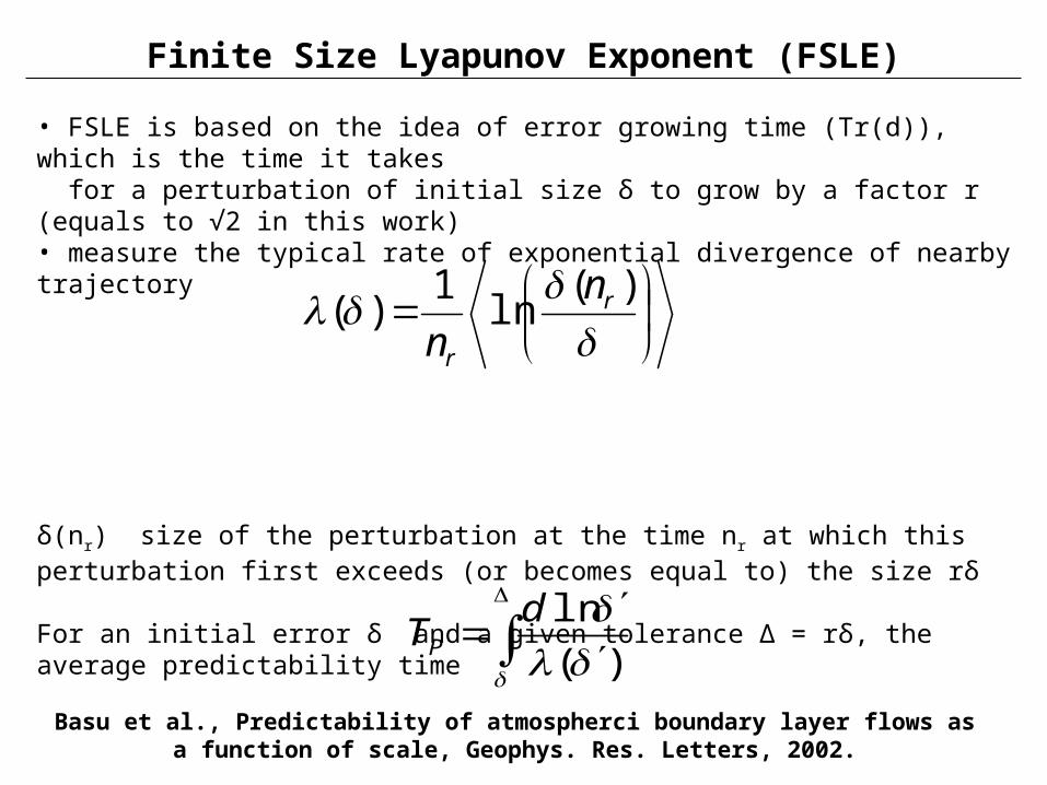
Finite Size Lyapunov Exponent (FSLE)

• FSLE is based on the idea of error growing time (Tr(d)), which is the time it takes for a perturbation of initial size δ to grow by a factor r (equals to √2 in this work)• measure the typical rate of exponential divergence of nearby trajectory

δ(nr) size of the perturbation at the time nr at which this perturbation first exceeds (or becomes equal to) the size rδ

For an initial error δ and a given tolerance ∆ = rδ, the average predictability time

)(

lndTP

)(

ln1

)( r

r

n

n

Basu et al., Predictability of atmospherci boundary layer flows as a function of scale, Geophys. Res. Letters, 2002.

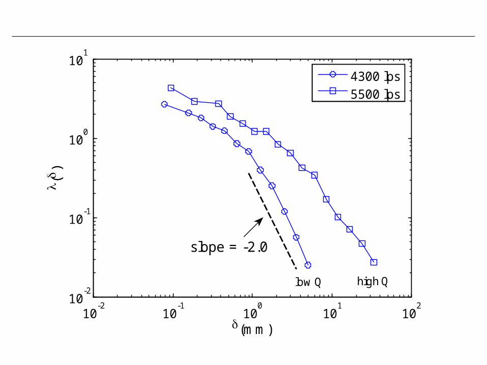
10-2

10-1

100

101

102

10-2

10-1

100

101

slope = -2.0

(mm)

( )

4300 lps5500 lps

low Q high Q

10-1

100

101

102

100

101

102

103

(mm)

TP (

sec)

4300 lps5500 lps low Q

high Q

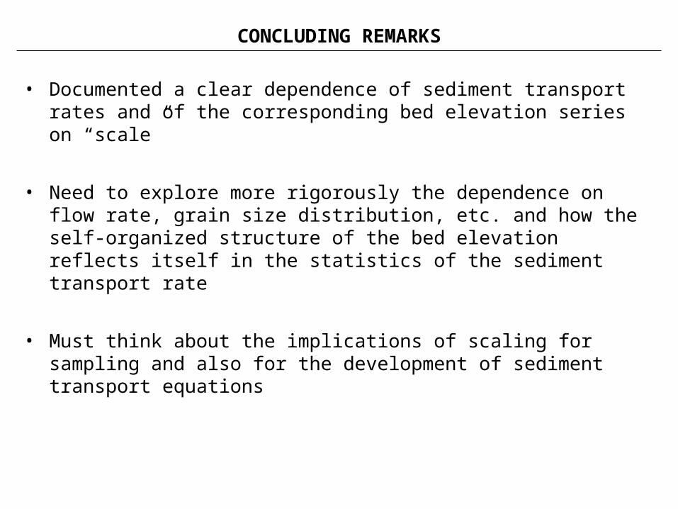
CONCLUDING REMARKS

• Documented a clear dependence of sediment transport rates and of the corresponding bed elevation series on “scale”

• Need to explore more rigorously the dependence on flow rate, grain size distribution, etc. and how the self-organized structure of the bed elevation reflects itself in the statistics of the sediment transport rate

• Must think about the implications of scaling for sampling and also for the development of sediment transport equations

References

Gangodagamage, C., E. Barnes, and E. Foufoula-Georgiou, Scaling in river corridor widths depicts organization in valley morphology, Geomorphology, doi:10.1016/j.geomorph.2007.04.414, 2007.

Lashermes, B. and E. Foufoula-Georgiou, Area and width functions of river networks: new results on multifractal properties, Water Resources Research, doi:10.1029/2006WR005329, 2007

Lashermes, B., E. Foufoula-Georgiou, and W. Dietrich, Channel network extraction from high resolution topograhy using wavelets, Geophysical Research Letters, in press, 2007.

Sklar L. S., W. E. Dietrich, E. Foufoula-Georgiou, B. Lashermes, D. Bellugi, Do gravel bed river size distributions record channel network structure?, Water Resources Research, 42, W06D18, doi:10.1029/2006WR005035, 2006.

Barnes, E. M.E. Power, E. Foufoula-Georgiou, M. Hondzo, and W.E. Dietrich, Scaling Nostic biomass in a gravel-bedrock river: Combining local dimensional analysis with hydrogeomorphic scaling laws, Geophysical Research Letters, under review.

THE END

0.2 0.25 0.3 0.35 0.4 0.45 0.50

5

10

15

20

25 H = 0.5

Rel

ativ

e fre

quen

cy

Transportation Distance

fbmsurrogates

10-2

10-1

100

101

10-4

10-3

10-2

10-1

100

101

( )

H = 0.5

slope = -2.0

0.4 0.6 0.8 1 1.2 1.4 1.6 1.8

x 10-3

0

2000

4000

6000

8000

10000

c1=0.7 c

2=0.2

Re

lativ

e fr

eq

ue

ncy

Transportation Distance

RWCsurrogates

10-5

10-4

10-3

10-2

10-1

10-4

10-3

10-2

10-1

100

( )

c1=0.7 c

2=0.2

slope= -2

Transportation Distance

• based on both the geometric and probabilistic aspects of point distributions • provide a measure of long term qualitative differences between any

two time series (x and y).

μij > 0 amount of material shipped from box Bi to box Bj

δij taxi cab metric normalized to the embedding dimension between the centres of Bi and Bj

b

jiijijqpMqpd

1,),(inf),(

RECALL

( ) ( ) ( ) ( )~q q

c ct k t t k t tx x+ ×D - ×D

( )2

1 2 2q

q c q ct = × - ×

• c2=0 monofractal (2)=2(1)

• all moments can be scaled with one parameter c1=H only

• CV is constant with scale

• c20 multifractalfractal (2)<2(1)

• need 2 parameters c1, c2 to scale pdfs

• CV decreases with increase in scale

{

{

1.

2.

(k t) =Sediment transported during a time period k t

t =Sampling interval

~

~

~

( )E k txD ×D

( )2

E k txD ×D

( )CV k txD ×D

( ) ( )1k t t×D

( ) ( )2k t t×D

( ) ( ) ( )2 2 1k t t t-×D

High-resolution temporal rainfall data

(courtesy, Iowa Institute of Hydraulic Research – IIHR)

~ 5 hrs

t = 10s

~ 1 hr

t = 5s