1

Extreme return-volume relationship in crypto currencies: tail dependence analysis Muhammad Naeem

Corresponding Author: University of Central Punjab. Email: naeem787@gmail.com

Abstract We explore the potential dependence between extreme return and volumes among different Crypto currencies, using various statistical models. Extreme dependence between return and volume in Bitcoin, Ethereum, Ripple and Litecoin has been investigated by using EGARCH-Copula approach. We have used Frank, Student-t, Clayton, Gumbel, Survival Clayton and SJC copulas. We use EGARCH model for return series and GARCH model for volume series. According to our finding, we have not found any significant symmetric dependence between return-volume. Because our parameter estimates, which is based on log likelihood, are not significant for student-t and Frank Copula. Further Our parameter for Bitcoin, Ripple and Litecoin of Clayton and SJC copulas are significant for return-volume relationship, which means that low return are followed by low volumes in case of Bitcoin, Ripple and Litecoin. On the other hand, our parameter for Ripple and Litecoin of Clayton and SJC copulas are significant, which means that for Ripple and Litcoin high return are followed by low volumes. According to our finding, Bitcoin, Ripple and Litecoin exhibited weak upper tail dependence between return and volume and strong low tail dependence for Ripple and Litecoin as compared to Bitcoin. Further, we have identified that the extremely low returns for Ripple and Litecoin are followed by relatively low volume then the Bitcoin and Ethereum, providing evidence against the leverage effect. Our investigation shows that investors (buyer or seller) are very careful in extreme market conditions for both Ripple and Litecoin. We have not found any evidence of upper tail or lower tail dependence for Ethereum. Keywords: Crypto, EGARCH-Copula model, return-volume, Negative returns, Upper tail dependence

1. Introduction

The development of internet technologies is dramatically changing the structure and nature of financial institutions. Internet technologies are enabling financial institutions to provide a products and services more effectively to customers. The technology changes with widening access give more advantage to customer by make a transaction more easily and practically. Emerging technology also give more advantage in the banking and financial area such as technology have changed the banking industry from paper and branch based banks to digitized and networked banking services by using an internet system. Therefore, new technology system was introduced many financial technologies product and service. One of the current new technologies introduced digital currencies. The aim of our paper is to study extreme return-volume relationship in four most representative cryptocurrencies: Bitcoin, Ethereum, Litecoin and Ripple. Because understanding the return–volume nexus can provide many useful signals for market participants to determine investment strategies or to rebalance their portfolios, a great number of theoretical and empirical studies have attempted to explain and explore this nexus from a number of different directions. The return and volume relationship has been analysed from many different point of views in the literature (e.g. Granger and Morgenstern, 1963, Crouch, 1970, Westerfield, 1977, Tauchen and Pitts, 1983, Rogalski, 1978, Clark, 1973). As investors

2

revise their reservation prices based on the arrival of new information to the market, trading volume had been used to measure disagreement among market participants by employing mixture models in Epps and Epps (1976). The level of trading volume increases as the degree of disagreement among traders spreads. Their model exhibits a positive causal relation running from trading volume to absolute stock returns. Jain and Joh (1988) found strong contemporaneous relation between trading volume and returns by using hourly common stock trading volume and return on NYSE. Further, they have also found lead-lag correspondence between trading volume and returns lagged up to 4 hours.

Moreover, trading volume-returns relation is higher for positive returns than for negative returns. The dynamic relationship between trading volume, volatility and returns of stock indices of nine national markets has been investigated by Chen et al. (2001). They found a positive dependence between trading volume and the absolute returns. They have also showed that trading volume provides some information about returns process. Gunduz and Hatemi (2005) explored the causal relationship between stock prices and volume of Hungary, Czech Republic, Russia, Poland and Turkey stock markets. Floros and Vougas (2007) had examined the relationship between trading volume and returns in Greek Stock Index Futures Market and found significant positive contemporaneous relationship between trading volume and returns in case of FTSE/ASE-20. Further, the results for FTSE/ASE Mid 40 do not provide any evidence of relationship between trading volume and returns. Furthermore, literature on return-volume dependence can be found in the papers of Kamath(2008), Attari et al. (2012) and Naeem et al.(2014).

There is a vivid debate in the literature about correlation between volatility and return volume. It is now a days accepted that they tend to show relatively strong upper tail dependence (see e.g. Rossi et al., 2013). Ning and Wirjanto (2009) found upper tail dependence in return and volume series of East Asian stock markets. However, Chen et al. (2001) explain that negative return in period t raises volatility in period t + 1. Further, explanation can be seen from Wagner (2012), that when volatility increases, risk increases and returns decrease. If we combine work of Rossi et al. (2013) and the fact mentioned in the paper by Chen et al. (2001) and Wagner (2012), then one should expect positive dependence between low return and volumes.

In this paper along with return-volume relationship, we also consider negative return-volume relationship, in order to explore the upper tail dependence between the negative return and volume. That is the dependence between the lower tail of return and upper tail of volume. Further, we consider return-volume dependence in order to analyse the difference between dependence parameter in both cases. Ning and Wirjanto (2009) used a copula approach to examine the extreme return-volume relationship in six emerging East-Asian equity markets. They used GARCH Copula approach. This is the first study, which consider crypto currencies for return-volume relationship by using EGARCH-Copula approach until now.

Our goal in this paper is to explore the extreme dependence between return and volumes of four crypto currencies. If crypto currencies returns are well described by the multivariate normal distribution, then the linear correlation is an appropriate dependence measure. However, in our case a simple exploratory and graphical analysis of both returns and volumes distributions suggest fat tails, heteroscedasticity, clustering and other non Gaussian features. Thus linear correlation might be deceptive in our analysis. Alternative measures of dependence based on copula methods combined with EGARCH model are considered here. Copula approach is widely used in quantitative finance literature. Here we combine copula modelling with a univariate EGARCH model for returns of crypto currencies in order to properly calibrate a joint model for returns and volumes. The remainder of this paper is organized as follows: section two introduces the EGARCH model. Section three describes copula methodology. Section four reports empirical results and section five conclude with summary of our finding.

3

2. EGARCH Model ARCH Model ARCH models based on the variance of the error term at time t depends on the realized values of the squared error terms in previous time periods. The model is specified as:

tt uy = (2.1) ( )tt h,0N~u

∑=

−α+α=q

1t

2itj0t uh

(2.2) This model is referred to as ARCH(q), where q refers to the order of the lagged squared returns included in the model. If we use ARCH(1) model it becomes

21t10t uh −α+α= (2.3)

Since th is a conditional variance, its value must always be strictly positive; a negative variance at any point in time would be meaningless. To have positive conditional variance estimates, all of the coefficients in the conditional variance are usually required to be non-negative. Thus coefficients must

be satisfy and . GARCH Model Bollerslev (1986) and Taylor (1986) developed the GARCH(p,q) model . The model allows the conditional variance of variable to be dependent upon previous lags; first lag of the squared residual from the mean equation and present news about the volatility from the previous period which is as follows:

∑ ∑= =

−− β+α+α=q

1i

p

1iiti

2iti0t huh

(2.4) In the literature most used and simple model is the GARCH(1,1) process, for which the conditional variance can be written as follows:

1t12

1t10t huh −− β+α+α= (2.5)

Under the hypothesis of covariance stationarity, the unconditional variance th can be found by taking the unconditional expectation of equation 5. We find that

hhh 110 β+α+α= (2.6) Solving the equation (2.5), we have

11

0

1h

β−α−α

= (2.7)

For this unconditional variance to exist, it must be the case that 111 <β+α and for it to be positive,

we require that 00 >α . Exponential GARCH

4

Exponential GARCH (EGARCH) proposed by Nelson (1991) which has form of leverage effects in its equation. In the EGARCH model the specification for the conditional covariance is given by the following form:

( ) ( )kt

ktr

kk

p

i it

iti

q

jjtjt h

uh

uhh

−

−

== =

=

=− ∑∑∑ +++=

1110 loglog γαβα

(2.9)

Two advantages stated in Brooks (2008) for the pure GARCH specification; by using ( )thlog even if the parameters are negative, will be positive and asymmetries are allowed for under the EGARCH formulation.

In the equation kγ represent leverage effects which accounts for the asymmetry of the model. While the basic GARCH model requires the restrictions the EGARCH model allows unrestricted estimation of the variance (Thomas and Mitchell2005:16).

If 0k <γ it indicates leverage effect exist and if 0k ≠γ impact is asymmetric. The meaning of leverage effect bad news increase volatility. Applying process of GARCH models to return series, it is often found that GARCH residuals still tend to be heavy tailed. To accommodate this, rather than to use normal distribution the Student’s t and GED distribution used to employ ARCH/GARCH type models (Mittnik et al. 2002:98). 2.1 Statistical Inference Parameter estimation of GARCH and EGARCH model is commonly carried out by using the maximum likelihood method with normality assumption for 𝜀𝜀𝑡𝑡. However, as mentioned by Kang et al. (2010) and Tang & Shieh (2006), the residuals estimated from the GARCH type model frequently exhibits lepto-kurtosis and asymmetry. To overcome these problems the Student-t distribution has been considered for the innovations process. Given the random variable 𝜀𝜀𝑡𝑡~𝑡𝑡𝜈𝜈(0,1, 𝜈𝜈) the log-likelihood function is defined as follows: log(𝐿𝐿;Θ) = 𝑇𝑇 �logΓ �

𝜈𝜈 + 12

� − log Γ�𝜈𝜈 2� � −12

log[𝜋𝜋(𝜈𝜈 − 2)]�

−��log𝜎𝜎2𝑡𝑡 + (1 + 𝜈𝜈) log�1 +𝜀𝜀2𝑡𝑡

𝜎𝜎2𝑡𝑡(𝜈𝜈 − 2)��

𝑇𝑇

𝑡𝑡=1

(2.10)

Matlab garchfit function has been used to estimate the parameters of the GARCH and EGARCH models. then the standardized residuals are calculated as follows. 𝜀𝜀𝑡𝑡 = 𝑟𝑟𝑡𝑡

�𝜎𝜎𝑡𝑡� (2.11)

3 The Copula Methodology Copula-based models provide a great deal of flexibility in modelling multivariate distributions. This allows the researcher to specify the models for the marginal distributions separately from the dependence structure (copula) that links them to form a joint distribution. From an inferential perspective the copula representation facilitates estimation of the model in stages, reducing the computational burden.

Several surveys of copula theory and applications have appeared in the literature to date: Nelsen (2006) and Joe (1997) are the most important text books on copula theory, providing detailed introductions to copulas and dependence modelling, with an emphasis on statistical foundations. Kurowicka and Joe (2011) represents an up-to-date survey on copula and vine-copula applications Cherubini, et al.(2004) present an introduction to copulas using methods from mathematical finance,

5

McNeil, et al. (2005) present an overview of copula methods for risk management. Patton (2009) presents a summary of applications of copulas to financial time series. Jondeau and Rockinger (2006) proposed a GARCH-Copula approach to measure the dependence structure of stock markets. It is well known that the analysis of dependence analysis, especially of extreme events, plays a crucial role in financial applications such as portfolio selection, Value-at-Risk, and international asset allocation.

A copula model is a way of constructing the joint distribution of a random vector 𝑋𝑋 =(𝑋𝑋1,⋯ ,𝑋𝑋𝑚𝑚). It is possible to show that there always exists an m-variate function C: [0, 1] m → [0, 1], such that

𝑭𝑭(𝑥𝑥1,⋯ , 𝑥𝑥𝑚𝑚) = 𝐶𝐶(𝐹𝐹1(𝑥𝑥1),⋯ ,𝐹𝐹𝑚𝑚(𝑥𝑥𝑚𝑚)) (3.1)

The copula function C is a cumulative distribution function (CDF) with uniform margins on [0, 1]: it binds together the univariate cumulative distribution functions F1, F2, and Fm to produce the m-variate CDF F. The three main properties are

i.) 𝐶𝐶(𝑥𝑥1, 𝑥𝑥2,⋯𝑥𝑥𝑚𝑚) is increasing in component 𝑥𝑥𝑖𝑖 ii.) 𝐶𝐶(1,⋯ ,1, 𝑥𝑥𝑖𝑖 , 1,⋯ ,1) = 𝑥𝑥𝑖𝑖 𝑓𝑓𝑓𝑓𝑟𝑟 𝑎𝑎𝑎𝑎𝑎𝑎 𝑖𝑖 = 1,⋯ ,𝑚𝑚, 𝑥𝑥𝑖𝑖 ∈ [0,1] iii.) For all (𝑎𝑎1,⋯ , 𝑎𝑎𝑚𝑚), (𝑏𝑏1,⋯ , 𝑏𝑏𝑚𝑚) ∈ [0,1]𝑚𝑚 𝑤𝑤𝑖𝑖𝑡𝑡ℎ 𝑎𝑎𝑖𝑖 ≤ 𝑏𝑏𝑖𝑖 one has

�⋯ �(−1)𝑖𝑖1+⋯+ℬ𝑚𝑚𝐶𝐶(𝑥𝑥1𝑖𝑖1 ,⋯ , 𝑥𝑥𝑚𝑚𝑖𝑖𝑚𝑚) ≥ 02

𝑖𝑖𝑚𝑚

2

𝑖𝑖1=1

where 𝑥𝑥𝑗𝑗1 = 𝑎𝑎𝑗𝑗 𝑎𝑎𝑎𝑎𝑎𝑎 𝑥𝑥𝑗𝑗2 = 𝑏𝑏𝑗𝑗 ∀ 𝑗𝑗 ∈ {1,⋯ ,𝑚𝑚 }

For any continuous multivariate distribution the copula representation is unique. If the marginal 𝐹𝐹1,⋯ ,𝐹𝐹𝑚𝑚 are not all continuous it can be shown that the joint CDF still have a copula representation although this representation is not unique. In the continuous case one can take derivatives of both side of Equation (3.1), we get the density representation of F:

𝑓𝑓(𝑥𝑥1, 𝑥𝑥2,⋯ , 𝑥𝑥𝑚𝑚) =𝜕𝜕𝑚𝑚𝐹𝐹(𝑥𝑥1,⋯ , 𝑥𝑥𝑚𝑚)𝜕𝜕𝑥𝑥1,⋯ , 𝜕𝜕𝑥𝑥𝑚𝑚

=𝜕𝜕𝑚𝑚𝐶𝐶(𝐹𝐹1(𝑥𝑥1),⋯ ,𝐹𝐹𝑚𝑚(𝑥𝑥𝑚𝑚))𝜕𝜕𝐹𝐹1(𝑥𝑥1)⋯𝜕𝜕𝐹𝐹𝑚𝑚(𝑥𝑥𝑚𝑚)

× 𝑓𝑓1(𝑥𝑥1) × ⋯× 𝑓𝑓𝑚𝑚(𝑥𝑥𝑚𝑚)

= 𝑐𝑐(𝐹𝐹1(𝑥𝑥1),⋯ ,𝐹𝐹𝑚𝑚(𝑥𝑥𝑚𝑚)) × �𝑓𝑓𝑖𝑖(𝑥𝑥𝑖𝑖)𝑚𝑚

𝑖𝑖=1

(3.2)

where 𝑐𝑐(𝑢𝑢1,⋯ ,𝑢𝑢𝑚𝑚) is the density of copula C, and 𝑓𝑓𝑖𝑖(𝑥𝑥𝑖𝑖) is the density of i-th margin. The joint use of GARCH and Copula models separates the temporal dependence, absorbed by the univariate GARCH structure, and the co-dependence among different variables, which is captured by the copula model. 3.1 Tail dependence and some bivariate copulas In this paper, we use the copula approach to measure the tail dependence between the return and volume among four crypto currencies, so we keep focus on the two-dimensional case only. We can use the tail dependence coefficient to measure the concordance between the extreme events of different random variables. It is expressed in terms of a conditional probability that the asset X will

6

incur a large loss (or gain), given that the asset Y also experiences a large loss (or gain). We consider two random variables X and Y, with joint continuous CDF F, copula C and margins FX; FY; the lower tail dependence and the upper tail dependence are defined as follows: 𝜆𝜆𝐿𝐿 = lim

𝑢𝑢→0+Pr(𝐹𝐹𝑋𝑋(𝑥𝑥) < 𝑢𝑢) |𝐹𝐹𝑌𝑌(𝑦𝑦) < 𝑢𝑢) = lim

𝑢𝑢→0+

𝐶𝐶(𝑢𝑢,𝑢𝑢)𝑢𝑢

(3.3)

𝜆𝜆𝑈𝑈 = lim

𝑢𝑢→1−Pr(𝐹𝐹𝑋𝑋(𝑥𝑥) > 𝑢𝑢) |𝐹𝐹𝑌𝑌(𝑦𝑦) > 𝑢𝑢) = lim

𝑢𝑢→1−

1 − 2𝑢𝑢 + 𝐶𝐶(𝑢𝑢,𝑢𝑢)1 − 𝑢𝑢

(3.4)

Intuitively, if 𝜆𝜆𝐿𝐿 and 𝜆𝜆𝑈𝑈 exist and fall in (0, 1], X and Y show lower or upper tail dependence. On the other hand, if 𝜆𝜆𝐿𝐿 and 𝜆𝜆𝑈𝑈 are equal to 0, one can say that the two variables are independent in the tails, so extreme events seem to occur independently. We can describe different tail dependence behaviour by choosing the appropriate copula model 3.1.1 Gaussian copula and Student t-copula These are symmetric and elliptical copulas. In the bivariate case the Gaussian copula is defined by the following expression: 𝐶𝐶𝜌𝜌𝐺𝐺(𝑢𝑢, 𝑣𝑣) = Φ𝜌𝜌�Φ−1(𝑢𝑢),Φ−1(𝑣𝑣)�

=

( )( )

( ) dsdttstsu v

−+−

−−

∫ ∫− −Φ

∞−

Φ

∞−2

22

2 122exp

121

1 1

ρρ

ρπ

(3.5)

where Φ𝜌𝜌the bivariate normal cumulative distribution function with linear correlation coefficient is 𝜌𝜌 ∈[0,1],Φ is the standard normal cumulative distribution function and Φ−1 is its inverse function. We can see that the bivariate Gaussian copula density is symmetrical, so it has weak capability to capture asymmetrical dependence. It implies that if we go far into the tail, the extreme events tend to be independent, even though we choose a very high correlation. The t-copula is corresponding to a Student t distribution. It is defined by:

𝐶𝐶𝜈𝜈,𝜌𝜌𝑡𝑡 = 𝑡𝑡𝜈𝜈,𝜌𝜌(𝑡𝑡𝜈𝜈−1(𝑢𝑢), 𝑡𝑡𝜈𝜈−1(𝑣𝑣))

=

Γ(𝜈𝜈2+1)

Γ(𝜈𝜈2)𝜋𝜋�1−𝜌𝜌2∫ ∫ 1 + −(𝑠𝑠2+2𝜌𝜌𝑠𝑠𝑡𝑡+𝑡𝑡2)

2(1−𝜌𝜌2)𝑎𝑎𝑑𝑑𝑎𝑎𝑡𝑡𝑡𝑡𝜈𝜈−1(𝑣𝑣)

−∞𝑡𝑡𝜈𝜈−1(𝑢𝑢)−∞ (3.6)

where 𝑡𝑡𝜈𝜈,𝜌𝜌 is the CDF of a two-dimensional t distribution with 𝜈𝜈 degree of freedom and correlation 𝜌𝜌. The t-copula also has symmetric shape, upper and lower tail dependence is identical, and it is determined by 𝜈𝜈 and 𝜌𝜌 . When 𝜈𝜈 gets large, then t-copula decays to a Gaussian copula. The expression of 𝜆𝜆𝐿𝐿 and 𝜆𝜆𝑈𝑈 follows:

𝜆𝜆𝐿𝐿 = 𝜆𝜆𝑈𝑈 = 2𝑇𝑇𝜈𝜈+1 ��(𝜈𝜈 + 1)(1 − 𝜌𝜌)

�𝜌𝜌 + 1�

(3.7)

where 𝑇𝑇𝜈𝜈+1 is the CDF of the scalar Student t distribution with 𝜈𝜈 + 1 degrees of freedom (Demarta and McNeil, 2005). 3.1.2 Archimedean Copulas Archimedean copulas are defined through their generator functions. Generally, if a function 𝜑𝜑: [0,1] →[0,∞] with the continuous derivative is decreasing and convex, it can be considered as a generator function of Archimedean copula. By definition an-dimensional Archimedean copula has the following

7

expression: 𝐶𝐶(𝑢𝑢1,𝑢𝑢2,⋯ ,𝑢𝑢𝑛𝑛) = 𝜑𝜑−1�𝜑𝜑(𝑢𝑢1) + 𝜑𝜑(𝑢𝑢2) + ⋯+ 𝜑𝜑(𝑢𝑢𝑛𝑛)�, different generator function creates different Archimedean copula. More details about generator function can be found in Joe(1997) and Nelsen(2006). In our case the copula function is defined by: 𝐶𝐶(𝑢𝑢, 𝑣𝑣) = 𝜑𝜑−1�𝜑𝜑(𝑢𝑢) + 𝜑𝜑(𝑣𝑣)� 𝑖𝑖𝑓𝑓 𝜑𝜑(𝑢𝑢) + 𝜑𝜑(𝑣𝑣) ≤ 𝜑𝜑(0) (3.8)

where 𝜑𝜑(𝑢𝑢) is a 𝐶𝐶2 function with 𝜑𝜑(1) = 0, 𝜑𝜑′ < 0,𝜑𝜑′′ > 0 . Examples of Archimedean copulas include the following: Clayton copula The Clayton copula has the following form: 𝐶𝐶(𝑢𝑢, 𝑣𝑣; 𝜌𝜌) = 𝑚𝑚𝑎𝑎𝑥𝑥[(𝑢𝑢−𝜌𝜌 − 𝑣𝑣−𝜌𝜌 − 1,0)]−1 𝜌𝜌 � 𝜌𝜌 ∈ (−1, +∞) ∖ {0} (3.9)

Where is the dependence parameter 𝜆𝜆𝐿𝐿 = 2

−1 𝜌𝜌� , 𝜆𝜆𝑈𝑈 = 0. When 𝜌𝜌 → 0, the margins tend to be independent, oppositely when 𝜌𝜌 → ∞, the margins tend to be strongly dependent. Clayton copula is asymmetric and it shows stronger low tail dependence. It can be proved that the components of a Gaussian copula are asymptotically independent. Frank copula The Frank copula is defined by:

𝐶𝐶(𝑢𝑢, 𝑣𝑣; 𝜌𝜌) = −1𝜌𝜌

log �(𝑒𝑒−𝜌𝜌𝑢𝑢 − 1)(𝑒𝑒−𝜌𝜌𝑣𝑣 − 1)

𝑒𝑒−𝜌𝜌 − 1− 1�

𝜌𝜌 ∈ (−∞, 0) ∪ (0, +∞)

(3.10)

Just like Gaussian copula, Frank copula is symmetric in both tails and it is not sensitive to

the relationship between the extreme negative values or between the extreme positive values. There is strong dependence in the centre of the distribution. This means that Frank copula fails to capture tail dependence behaviour and it suggests that it is suited to use when the tail dependence is relatively weak. Gumbel copula The Gumbel copula is an asymmetric extreme value copula, which takes the following expression: 𝐶𝐶(𝑢𝑢, 𝑣𝑣;𝜌𝜌) = 𝑒𝑒𝑥𝑥𝑒𝑒[(−𝑎𝑎𝑎𝑎𝑢𝑢)𝜌𝜌 + (−𝑎𝑎𝑎𝑎𝑣𝑣−𝜌𝜌)]−1 𝜌𝜌 � 𝜌𝜌 ∈ [1,∞)

(3.11)

where 𝜌𝜌 is a dependence parameter that describes different dependence behaviour, 𝜆𝜆𝐿𝐿 = 0, 𝜆𝜆𝑈𝑈 =2 − 2

1 𝜌𝜌� . When 𝜌𝜌 → ∞ the margins show totally dependence, while 𝜌𝜌 = 1 corresponds to independence case. Unlike the Clayton copula, Gumbel copula deals with upper tail dependence. If two margins perform simultaneous extreme upper tail values, the Gumbel copula should be an appropriate considerable choice. The Symmetrized Joe–Clayton copula Joe (1997) constructs the copula by taking a particular Laplace transformation of Clayton’s copula. The Joe–Clayton copula is:

8

( ) ( )[ ] ( )[ ]{ } kkkLU

JC vuvuC/1/1

1111111,|,

−−−+−−−−=

−−− γγγττ

(3.12)

where )2(log1

2Uk

τ−=

, )(log1

2Lτ

γ −=

and ( )1,0∈iτ are the measures of the upper- and lower-tail dependencies respectively. Patton's (2006a) modified Joe–Clayton (JC) copula for which the density is as follows.

( ) ( ) ( )( )1,|1,1,|,21,|, −++−−+= vuvuCvuCvuC LU

JCLU

JCLU

SJC ττττττ (3.13)

The SJC copula is symmetric when 𝜏𝜏𝑈𝑈 = 𝜏𝜏𝐿𝐿 and asymmetric otherwise. 3.2 Copula parameters estimation Most of the methods for copula parameter estimation are related to Maximum Likelihood procedures. The standard ML method which estimates both marginal parameters and copula parameters simultaneously is also named one step method. Mashal and Naldi (2002) noted that this method is computational costly, and when the data sets are not sufficiently large, the ML estimators seem to be ineffective. The inference function for margins method (IMF) is based on the work of Joe and Xu (1996). The estimation procedure is split in two steps; first one estimates the parameters of the marginal distributions. In the second step one tries to estimates of the copula parameters, conditionally on the values of estimates obtained at the first step. This approach offers computational convenience, although it may be sensitive to the choice of marginal distributions form. A poor estimator of the copula parameter might be a consequence of an inappropriate marginal distribution. There is also an alternative, two steps method, named Canonical Maximum Likelihood (CML). Unlike IMF method, in the ’CML’ approach the transformation is done by using empirical CDF function to obtain uniform margins, which are used in copula parameters estimation.

Given two time series {𝑋𝑋}𝑡𝑡=1𝑇𝑇 and {𝑌𝑌}𝑡𝑡=1𝑇𝑇 , let Ω be the parameter space, 𝑎𝑎𝑥𝑥 ∈ Ω, 𝑎𝑎𝑦𝑦 ∈Ω denote marginal parameters for X and Y, while 𝜃𝜃 ∈ Ω denotes copula parameters. From Equation 3.2, the log maximum likelihood function can be obtained as:

(𝛼𝛼𝑥𝑥 ,𝛼𝛼𝑦𝑦 ,𝜃𝜃;𝑋𝑋,𝑌𝑌) = �𝑎𝑎𝑎𝑎𝑐𝑐�𝐹𝐹𝑋𝑋(𝑥𝑥𝑡𝑡;𝛼𝛼𝑥𝑥),𝐹𝐹𝑌𝑌�𝑦𝑦𝑡𝑡;𝛼𝛼𝑦𝑦�; 𝜃𝜃� 𝑇𝑇

𝑡𝑡=1

+�(𝑎𝑎𝑎𝑎𝑓𝑓𝑋𝑋(𝑥𝑥𝑡𝑡;𝛼𝛼𝑥𝑥) + 𝑎𝑎𝑎𝑎𝑓𝑓𝑦𝑦(𝑦𝑦𝑡𝑡 ,𝛼𝛼𝑦𝑦))𝑇𝑇

𝑡𝑡=1

(3.14)

Here we sketch the necessary inferential steps. Step 1 Estimating parameters of the marginal distributions, 𝛼𝛼𝑥𝑥 and 𝛼𝛼𝑦𝑦.

𝛼𝛼�𝑥𝑥 = 𝑎𝑎𝑟𝑟𝑎𝑎max𝛼𝛼𝑥𝑥

�𝑎𝑎𝑎𝑎𝑓𝑓𝑋𝑋(𝑥𝑥𝑡𝑡 ,𝛼𝛼𝑥𝑥)𝑇𝑇

𝑡𝑡=1

(3.15)

𝛼𝛼�𝑦𝑦 = 𝑎𝑎𝑟𝑟𝑎𝑎max

𝛼𝛼𝑦𝑦�𝑎𝑎𝑎𝑎𝑓𝑓𝑌𝑌(𝑦𝑦𝑡𝑡 ,𝛼𝛼𝑦𝑦)𝑇𝑇

𝑡𝑡=1

(3.16)

9

Step 2 Estimating the copula parameters by using the estimator 𝛼𝛼�𝑥𝑥 and 𝛼𝛼�𝑦𝑦 obtained in step 1.

𝜃𝜃� = argmax𝜃𝜃

�𝑎𝑎𝑎𝑎𝑐𝑐(𝐹𝐹𝑋𝑋(𝑥𝑥𝑡𝑡;𝛼𝛼�𝑥𝑥),𝐹𝐹𝑌𝑌�𝑦𝑦𝑡𝑡;𝛼𝛼�𝑦𝑦�; 𝜃𝜃)𝑇𝑇

𝑡𝑡=1

(3.17)

The copula parameters were estimated by employing the maximum likelihood method

described in Equation 3.17. For the IMF estimation, a MATLAB copula toolbox written by Patton (2008) has been used.

4. Empirical studies and analysis 4.1 Primary Data Analysis In empirical studies, we choose daily prices and corresponding trading volume series of four crypto currencies, Bitcoin, Ethereum, Ripple and Litecoin. These data ranges from 8 August, 2015 to 25 February 2018. Figure I illustrates the relative price movements of each crypto currency. We take the daily log returns defined as 𝑅𝑅𝑡𝑡 = 100 × log�𝑒𝑒𝑡𝑡 𝑒𝑒𝑡𝑡−1� � which can be seen in Figure II.

Figure I: Daily Closing Prices of Each crypto currency

10

Figure II: logarithm Return of each crypto currency series The preliminary descriptive statistics of the data are presented in Table 1. Hodrick and Prescott (1997) filter have been used to remove the trend from the log-volume series. As shown in Table 1, the kurtosis of each index is greater than 3 and the skewness is not zero, which both suggest that presence of fat tails and leptokurtosis. Table 1: Descriptive statistics of the sample data

Descriptive Statistics Bitcoin Ethereum Ripple Litecoin observation 933 933 933 933

mean 0.003875 0.0075347 0.005056163 0.00434 std 0.041071 0.07313 0.08096 0.06013 max 0.225119 0.412337 1.02736 0.51035 min -0.207529 -0.315469 -0.616273 -0.3952 skewnss -0.275847 0.522313 3.1192936 1.45066 kurtosis 8.294972 7.317244 41.5123 16.5257 Jarque-Bera _ 5.9226 1.1006e+003 766.1754 5.9109e+004 7.4e+003 Q(20)_ cv_31.4104 25.4970 36.7330 56.1689 40.2091 ARCH-LM _ 3.8415 50.3921 32.4973 77.4362 20.9612 Adjusted Volume mean -0.0000 -0.0000 -0.0000 -0.0000 std 0.469081 0.760698 0.9111 0.73611 skewnss 0.521130 0.0732621 0.2169564 0.36286 kurtosis 3.1198463 2.88268776 3.2311953 3.10091 Jarque-Bera 42.7885 1.3696 9.3973 20.8705 Q(20) 2.6395e+003 3.1373e+003 2.5809e+003 3.2e+003 ARCH-LM 282.7823 323.5122 339.7724 332.9092

Notes: Table 1 shows Jarque-Bera is test statistics for the test of normality. Q (20) is the Ljung-Box statistic for serial correlation in the return and adjusted volumes computed with 20 lags. ARCH-LM is the Engel’s LM test for heteroscedasticity, conducted using 20 lags. * A rejection of the null hypothesis at 5% level

11

The order for the ARMA part has been chosen, after careful inspection of ACF and PACF of both return and de-trended volume series. Parameter estimation for return and volume are reported in Table 2. One motivation for using ARMA-GARCH type model is the inspection of ACF of return and volume and ACF of squared return in Figure III. After performing ARCH test over the series of residuals we proceed with the selection of order of GARCH model. Here we have applied EGARCH and GARCH type models for return and de-trended volume series respectively. Further, residuals and squared residuals series do not possess significant autocorrelation for both return and volume series as it can be seen in Figures IV and V.

Figure III: Autocorrelation of Squared Returns

Figure IV: ACF of squared standardized residuals of Returns The test shows that residuals are approximately i.i.d series, therefore copula approach can

be applied to the residuals after getting student t CDF from the residuals. We use EGARCH and

12

GARCH model to fit the marginal distribution of each return and each volume series. Estimated parameters for each type of model are given in Table 2.

Table 2: Parameter estimation of GARCH and EGARCH model GARCH for Volume EGARCH for Returns Parameters Bitcoin Ethereum Ripple Litecoin Bitcoin Ethereum Ripple Litecoin Mean Equation

Μ -0.0104 (0.0102)

-0.0000 (0.0159)

-0.0233 (0.0179)

-0.0387*** (0.0135)

0.0027*** (0.0005)

0.0000 (0.0015)

-0.0033*** (0.0008)

-0.0000 (0.0005)

ϕ1 0.7566*** (0.0240)

0.7778*** (0.0226)

0.7841*** (0.0207)

0.7961*** (0.0186)

-0.0698** (0.0273)

-0.0114 (0.0336)

-0.0459* (0.0278)

-0.1167*** (0.0223)

Variance Equation

Ω 0.0140*** (0.0069)

0.0000 (0.0000)

0.1471 (0.0932)

0.0048 (0.0035)

-0.0560 (0.0464)

-0.4447 (0.1192)

-0.2607*** (0.0968)

-0.0334* (0.0193)

α1 0.1061*** (0.0351)

0.0198*** (0.0073)

0.0813* (0.0506)

0.0424*** (0.0165)

0.4156*** (0.1164)

0.5374*** (0.0879)

0.9312** (0.5111)

0.2627*** (0.0899)

Β 0.7621*** (0.0833)

0.9793*** (0.0073)

0.4704 (0.3086)

0.9355*** (0.0273)

0.9902*** (0.0068)

0.9159*** (0.0215)

0.9372*** (0.0136)

0.9959*** (0.0033)

γ1 — —

— —

— —

---- ---

0.1357** (0.0533)

-0.0197 (0.0442)

-0.1028 (0.1149)

0.1289*** (0.0461)

Ν 12.6094** (5.4331)

53.02 (87.3)

7.7075*** (1.8644)

5.1680*** (0.8592)

2.4064*** (0.2702)

3.2*** (0.4791)

2.0961*** (0.1094)

2.1896*** (0.1240)

Notes:Table 2 reports the estimated parameters for EGARCH and GARCH models for returns and volumes respectively, together with standard errors (in parentheses). * indicates significance at 10% level. ** indicates significance at 5% level. *** indicates significance at 1% level. 4.2 Marginal Distribution Models AR(1)-EGARCH(1,1) models were estimated for all return series by selecting lag order for mean equation by the inspection of ACF and PACF, maintaining the conditional variance equation as EGARCH(1,1) model. Further, AR (1)-GARCH (1, 1)-t models have been applied to volume series. MATLAB function ’garchfit’ has been used to estimate the parameters of the GARCH and EGARCH models. Parameters estimates can be seen in Table 2. In Table 2, most of the coefficients in the conditional variance equation are significant. Engle’s ARCH test has been applied to the square of the standardized residuals. The test fails to reject the null hypothesis of no ARCH effect1.

1 Results of the test will be provided upon request

13

Figure V: ACF of squared standardized residuals of Volumes

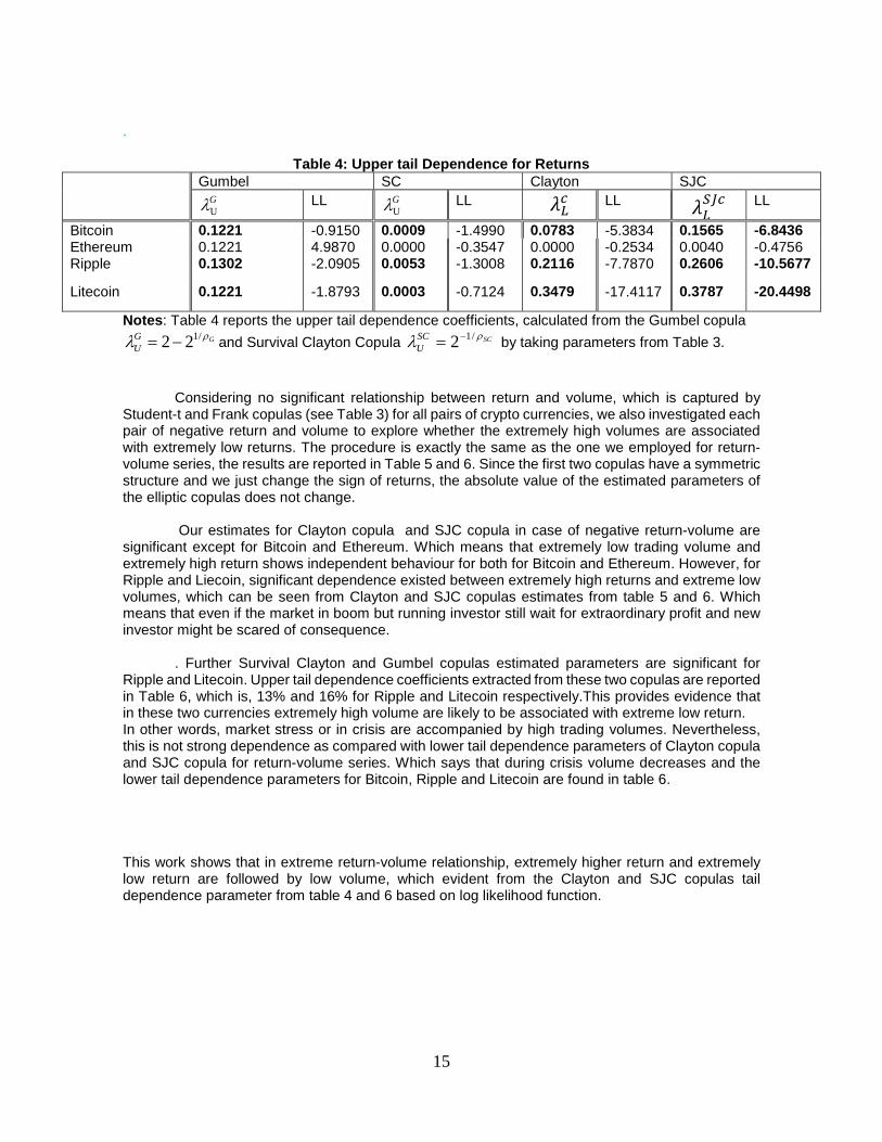
4.3 Copula Parameter Estimation We are interested in the dependence structure between the crypto currencies returns and trading volumes. Our main goal being to explore the extreme dependence between return and volumes. We employed 6 copulas in our analysis, the first two, namely, Student-t, and Frank copula, are symmetric and they have been used to analyse the dependence structure between each pair of return and volume. The other have been used to analyse the asymmetric dependence between return and volume, as reported in literature (Karpoff, 1987 and Gervais et al., 2001). The asymmetric copulas are able to capture potential difference between lower and upper tail. The parameter estimates for each copula have been reported in Table 3 which is based on Log Likelihood function. Table 3 exhibits there is no significant symmetric relationship between return and trading volume as evident from the parameter estimates of Student-t and Frank copula for all four currencies. Now we focus on the potential asymmetry in the return-volume dependence by adopting Clayton, Survival Clayton, Gumbel and SJC copulas. We can see from Table 3 that the parameters of the Clayton and SJC copulas are significant for Bitcoin, Ripple and Litecoin, which suggest the presence of lower tail dependence. It implies that extremely low returns are associated with low volumes in case of Bitcoin, Ripple and Litecoin. Which means during the market stress of crypto currencies most of the investor still wanted to keep the crypto currencies specially Ripple and Litecoin as compared to Bitcoin. Possible reason might be that Ripple and Litecoin are cheaper and Bitcoin is expensive. Therefore, during the market stress if the loss is not that much then it is better to wait rather than selling. For some investor Bitcoin proves to be a lottery and some day if it could be true for Ripple and Litecoin to reach at the level of Bitcoin might be the reason of low trading volume during market stress. Further new investor always careful in investing during market stress. At the same time, the parameters of the Survival Clayton are significant for all pairs except Ethereum and Litecoin. Further, if we check the parameters of the Gumbel copula, then all the parameters are found to be significant for all pair of return and volume. The upper tail dependence coefficients for Gumbel and Survival Clayton copula are reported in Table 4, which have been extracted from the EGARCH-Copula model.

14

Table 3: Copula estimates of return-volume dependence Bitcoin Ethereum Ripple Litecoin Student-t copula ρ 0.0537

(0.0706) 0.0575 (1.453)

-0.0047 (0.1148)

-0.0620 (0.0913)

ν 5.3843*** (1.6130)

100*** (0.0007)

3.9212*** (0.8293)

2.5179*** (0.3609)

AIC -7.0693 -0.5882 -12.1199

-25.9357

Frank Copula ρ 0.4000

(.3728) 0.3242 (0.2527)

1.0961 (0.7426)

1.0000e-004 (10.09)

AIC -0.5661 -0.8215 -0.3595 0.0001 Clayton Copula ρ 0.2721***

(0.0802) 0.0525

(0.0740) 0.4463

(0.0956) 0.6565

(0.0961) AIC -5.3834 -0.2534 -7.7870 -17.4117 Survival Clayton Copula ρ 0.0980***

(0.0601) 0.0377 (0.0460)

0.1323** (0.0820)

0.0857 (0.0742)

AIC -1.4990 -0.3547 -1.3008

-0.7124

Gumbel Copula ρ 1.1000***

(0.0505) 1.1000*** (0.0456)

1.1076*** (0.0536)

1.1000*** (0.0564)

AIC -0.9150 4.9870 -2.0905 -1.8793

Symmetrised Joe-Clayton copula

Tu 0.0002 (0.0023)

0.0000 (0.0000)

0.0445 (0.0572)

0.0046 (0.0259)

T_L 0.1565*** (0.0605)

0.004 (0.051)

0.2606*** (0.0574)

0.3787*** (0.0461)

AIC -6.8436 -0.4756 -10.5677

-20.4498

Notes:Table 3 reports the estimates of parameters of six copulas for each pair of return and volume, together with standard errors (in parentheses) and the values of Akaike Information Criteria(AIC). *** indicates significance at 1% level. ** indicates significance at 5% level

We can see from Table 4 that relatively weak upper tail dependence is existed in return and volume of the Bitcoin, Ripple and Litecoin but there is no upper tail dependence existed in Ethereum. Which means that when during the time of market boom there is evidence of trading, but it is not strong evidence according log likelihood function. On the other hand, for Ethereum extremely high return and extremely high volume are independent.

15

.

Table 4: Upper tail Dependence for Returns Gumbel SC Clayton SJC

GUλ LL G

Uλ LL 𝜆𝜆𝐿𝐿𝑐𝑐 LL 𝜆𝜆𝐿𝐿𝑆𝑆𝑆𝑆𝑐𝑐

LL

Bitcoin 0.1221 -0.9150 0.0009 -1.4990 0.0783 -5.3834 0.1565 -6.8436 Ethereum 0.1221 4.9870 0.0000 -0.3547 0.0000 -0.2534 0.0040 -0.4756 Ripple 0.1302 -2.0905 0.0053 -1.3008 0.2116 -7.7870 0.2606 -10.5677

Litecoin 0.1221 -1.8793 0.0003 -0.7124 0.3479 -17.4117 0.3787 -20.4498

Notes: Table 4 reports the upper tail dependence coefficients, calculated from the Gumbel copula GG

Uρλ /122−= and Survival Clayton Copula SCSC

Uρλ /12−= by taking parameters from Table 3.

Considering no significant relationship between return and volume, which is captured by Student-t and Frank copulas (see Table 3) for all pairs of crypto currencies, we also investigated each pair of negative return and volume to explore whether the extremely high volumes are associated with extremely low returns. The procedure is exactly the same as the one we employed for return-volume series, the results are reported in Table 5 and 6. Since the first two copulas have a symmetric structure and we just change the sign of returns, the absolute value of the estimated parameters of the elliptic copulas does not change.

Our estimates for Clayton copula and SJC copula in case of negative return-volume are

significant except for Bitcoin and Ethereum. Which means that extremely low trading volume and extremely high return shows independent behaviour for both for Bitcoin and Ethereum. However, for Ripple and Liecoin, significant dependence existed between extremely high returns and extreme low volumes, which can be seen from Clayton and SJC copulas estimates from table 5 and 6. Which means that even if the market in boom but running investor still wait for extraordinary profit and new investor might be scared of consequence.

. Further Survival Clayton and Gumbel copulas estimated parameters are significant for

Ripple and Litecoin. Upper tail dependence coefficients extracted from these two copulas are reported in Table 6, which is, 13% and 16% for Ripple and Litecoin respectively.This provides evidence that in these two currencies extremely high volume are likely to be associated with extreme low return. In other words, market stress or in crisis are accompanied by high trading volumes. Nevertheless, this is not strong dependence as compared with lower tail dependence parameters of Clayton copula and SJC copula for return-volume series. Which says that during crisis volume decreases and the lower tail dependence parameters for Bitcoin, Ripple and Litecoin are found in table 6. This work shows that in extreme return-volume relationship, extremely higher return and extremely low return are followed by low volume, which evident from the Clayton and SJC copulas tail dependence parameter from table 4 and 6 based on log likelihood function.

16

Table 5: Copula estimates for negative return-volume dependence

Bitcoin Ethereum Ripple Litecoin Student-t copula ρ -0.0537

(0.0706) -0.0575 (1.453)

0.0047 (0.1148)

0.0620 (0.0913)

ν 5.3843*** (1.6130)

100*** (0.0007)

3.9212*** (0.8293)

2.5179*** (0.3609)

AIC -7.0693 -0.5882 -12.1199 -25.9357 Frank Copula ρ 0.0001

(0.3661) 0.0001 (0.2501)

0.6920 (1.7225)

1.5283 (0.5600)

AIC 0.0003 0.0005 0.0408 -1.4783 Clayton Copula ρ 0.0001

(0.0889) 0.0001

(0.0658) 0.3838*** (0.0984)

0.5738*** (0.0974)

AIC 0.0005 0.0020 -4.8962 -11.9307 Survival Clayton Copula ρ 0.0001

(0.0709) 0.0001 (0.0606)

0.0975 (0.0926)

0.1163 (0.0878)

AIC 0.0017 0.0021 -0.5199 -0.8609

Gumbel Copula ρ 1.1000***

(0.0518) 1.1000*** (0.0470)

1.1058*** (0.0556)

1.1413*** (0.0547)

AIC 5.1033 11.3945 -1.8298 -3.5921

Symmetrised Joe-Clayton copula

Tu 0.0000 (0.0000)

0.0000 (0.9121)

0.0471 (0.0607)

0.0406 (0.0613)

T_L 0.0557 (166.25)

0.0000 (0.5021)

0.2272*** (0.0583)

0.3362*** (0.0510)

AIC 0.0564 1.4290 -7.4721 -15.7087

Notes:Table 5 reports the estimates of parameters of six copulas for each pair of negative return and volume, together with standard errors (in parentheses) and the values of Akaike Information Criteria(AIC). ***indicates significance at 1% level. Leverage effect is referred to an asymmetric negative correlation between return and the volatility. In our study we found no leverage effect not only from the EGARCH model but also from the return volume dependence. As we have already explained that the volumes are positively associated with volatility, and further extreme low return are also positively associated with volatility. However in case of crypto currencies results are contradictory from most of the paper in the literature. Some paper says that if volatility increase then volume is increase and some paper says if the return increase then volume is also increase but both of these are not true in case of crypto currencies. We found that in

17

case Ripple and Litecoin higher return and low return are followed by low volume that is a new information in case of crypto currencies until now.

Table 6: Upper tail dependence coefficients for negative returns and volume

Gumbel SC Clayton SJC GUλ LL 𝜆𝜆𝑈𝑈𝑆𝑆𝑆𝑆 LL 𝜆𝜆𝐿𝐿𝑐𝑐 LL 𝜆𝜆𝐿𝐿

𝑠𝑠𝑗𝑗𝑐𝑐 LL

Bitcoin 0.1221 5.1033 0.0000 0.0017 0.0000 0.0005 0.0557 0.0564 Ethereum 0.1221 11.3945 0.0000 0.0021 0.0000 0.0020 0.0000 1.4290 Ripple 0.1284 -0.18298 0.0008 -0.5199 0.1643 -4.8962 0.2272 -7.4721

Litecoin 0.1645 -3.5921 0.0026 -0.8609 0.2988 -11.9307 0.3362 -15.7087 Notes: Table 6 reports the upper tail dependence coefficients, calculated from the Gumbel copula

GGU

ρλ /122−= and Survival Clayton Copula SCSCU

ρλ /12−= by taking parameters from Table 5. 5. Conclusion We have analyzed the dependence structure between return-volume and negative return and volume. Our analysis was based on modeling dependence structure via EGARCH-Copula models. We have used both tail independent and tail dependent copulas. Based on Log likelihood function we found that Clayton and SJC Copulas provide better results for both return-volume and negative return-volume relationship. According to our finding, Bitcoin, Ripple and Litecoin showed weak upper tail dependence between return and volume and strong low tail dependence for Ripple and Litecoin as compared to Bitcoin. We found that in case of Ripple and Litecoin extremely high return and extremely low returns are followed by low volume. For Bitcoin we found evidence of lower tail dependence between return and volume but no evidence of upper tail dependence. For Ethereum we found neither upper nor low tail dependence for both types of return.

18

References Attari, M.I.J., Rafiq, S. and Awan, M.H., 2012, The dynamic relationship between stock volatility and

trading volume. Asian Economic of PhD Thesis and Financial Review, vol. 2, issue 8, 1085-1097

Baillie, R.T., Bollerslev, T. and Mikkelsen, H.O., 1996, fractionally integrated generalized autoregressive conditional heteroscedasticity. Journal of Econometrics 74, 3-30.

Balduzzi,P., Kallal,H. and Longin, F.,1996, Minimal returns and the breakdown of price-volume relation. Economics Letters 50, 265-269.

Bollerslev, T., 1986, Generalized Autoregressive conditional heteroscedasticity. Journal of Econometrics 31:307-327

Breidt, F.J., Crato N. and de Lima P.J.F., 1998, The detection and estimation of long memory in stochastic volatility. Journal of Econometrics 83, 325-348.

Chen, G., Firth, M. and Rui, 0. M., 2001, The dynamic relation between stock returns, trading volume and volatility. The Financial Review38, 153-174.

Cherubini, U., Luciano, E., Vecchiato, W., 2004, Copula method in Finance. John Wiley & Son Ltd.

Clark, P. ,1973, A subordinated stochastic process model with finite variance for speculative prices. Econometrica 41, No. 1, 135-155.

Crouch, R., 1970, The volume of transaction and price changes on the New York Stock Exchange. Financial Analysts Journal, July-Aug., 104-109

Demarta, S. and McNeil, A.J., 2005, The t copula and related copulas. International Statistical Review, 73(1), 111-129.

Deng, L., Ma, C. and Yang, W., 2011, Portfolio optimization via pair copula-GARCHEVT-CVaR model. Systems Engineering Procedia 2, 171-181

Epps, T. W., and Epps, M. L., 1976, The stochastic dependence of security price changes and transaction volumes: implications for the mixture of distributions hypothesis. Econometrica 44, 305-321.

Engle, R.F., 1982, Autoregressive conditional heteroscedasticity with estimates of the variance of United Kingdom inflation. Econometrica 50,987-1007

Floros, C. and Vougas, D., 2007, Trading volume and returns relationship in Greek stock index futures market: GARCH vs. GMM. International Research Journal of Finance and Economics 12, 98-115.

Gervais, S., Kaniel, R.,Mingelgrin, D. ,2001, High-volume return premium. Journal of Finance 56, 877-919.

Goudarzi, H., 2010, Modelling long memory in the Indian Stock Market using fractionally integrated E-garch model. International Journal of Trade, Economics and Finance 1, No.3, 231-237.

Baillie, R. T. ,1996, Fractionally intergrated model. Journal of Econometrics , 3-30. Granger, C. and Morgenstern, o., 1963, Spectral analysis of New York Stock Market prices.

Kyklos 16, 1-25. Gunduz, L. and Hatemi-J, A., 2005, Stock price and volume relation in emerging markets.

Emerging Markets Finance and Trade 41, 29-44.

19

Jain, P.C. and Joh, G.H., 1988, The dependence between hourly prices and trading volume. The Journal of Financial and Quantitative Analysis 23, 269-283.

Joe, H. and Xu, J.J.,1996, The estimation method of inference functions for margins for multivariate models, Technical Report,166,Department of Statistics, University of British Columbia, Canada.

Joe, H., 1997, Multivariate models and dependence concepts, London: Chapman&Hall. Jondeau, E. and Rockinger, M., 2002, Conditional dependency of financial series: the

copula-GARCH model. International Center for Financial Asset Management and Engineering, FAME Research Paper Series rp69.

Jondeau, E. and Rockinger, M., 2006, The copula-GARCH model of conditional depen-dencies: An international stock market application. Journal of International Money and Finance 25, 827-853.

Kamath, R. R., 2008, The price-volume relationship in the Chilean stock market. Interna-tional Business and Economic Research Journal 7, 7-13.

Kang, S.H., Cheong, C.C. and Yoon, S.M., 2010, Long memory volatility in Chinese stock markets, Physica A 389, 1425-433.

Kang, S.H. and Yoon, S., 2012,. Dual long memory properties with skewed and fat-tail distribution. International Journal of Business and Information 7(2).

Karpoff, J.M., 1987, The relation between price change and trading volume: a survey. Journal of Financial Research and Quantitative Analysis 22, March 1987, 109-126.

Karpoff, J.M., 1988, Costly short sales and the correlation of return with volume. The Journal of Financial Research, 11, No.3, 173-188.

Kartsaklas, A. and Karanasos, M., 2013, Long run dependencies in stock volatility and trading volume. Working Paper, 13-16, Brunel University, London, UK.

Kasman, A. and Torun, E., 2007, Long memory in the Turkish Stock Market return and volatility. Central Bank Review, 13-27.

Kumar, A. , 2004, Long memory in stock trading volume: Evidence from Indian Stock Market .Indira Gandhi Institute of Development Research-Economics.

Mashal, R. and Naldi, M., 2002, Pricing multiname credit derivatives:Heavy tailed approach. Quantitative Credit Research Quarterly, 3107-3127.

MecNeil, A. J., Frey, R. and Embrechts, P., 2005, Concepts, techniques and tools, Quantitative Risk Management, Princeton University Press.

Navarro J.,R., Tamangan, R., Guba-Natan, N. , Ramos, E. and Guzman, A.D. ,2006, The identification of long memory process in the Asian-4 stock markets by fractional and multi-fractional Brownian motion. The Philippine Statistician 55 .No.1-2, 65-83.

Nelson, R.B, 2006, An introduction to copulas, New York: Springer-Verlag. Ning, C. and Wirjanto, T.S., 2009, Extreme return-volume dependence in East-Asian stock

markets: A copula approach. Finance Research Letters 6(4), 202-209. Patton, A. J., 2006, modelling asymmetric exchange rate dependence. International

Economic Review 47(2), 527-556. Patton, A. J. (2008), Copula toolbox for MATLAB, available for download at: http://public.econ.duke.edu/ ap172/code.html. Puri,T.N., 2008, Asymmetric volume-return relation and concentrated trading in LIFFE

Futures. European Financial Management 14, No.3, 528-563. Rogalski, R., 1978, The dependence of prices and volume. Review of Economics and

Statistics 58, 268-274. Sklar, A., 1959, Fonctions de répartition á n dimensions et leurs marges. Publication de

l'Institut de Statistique de l'Universite de Paris 8, 229-231. Sklar, A., 1973, Random variables, joint distribution functions, and copulas. Kybernetika

9, .449-460. Sheppard, K., 2013, Oxford MFE Toolbox. Available at:

http://www.kevinsheppard.com/wiki/MFE_Toolbox.

20

Tan, S. and Khan, M.T.I., 2010, Long memory features in return and volatility of the Malaysian Stock Market. Economics Bulletin 30, No.4, 3267-3281.

Tang T.L. and Shieh, S.J., 2006, Long memory in stock index future markets: A value at risk approach. Physica A: Statistical Mechanics and it Applications, vol.366, 437-448.

Tauchen, G. and M. Pitts., 1983, The price variability-volume relationship on speculative markets. Econometrica 5, 485-505.

Westerlield, R., 1977, The distribution of common stock price changes: An application of transactions time and subordinate stochastic models. Journal of Financial and Quantitative Analysis 12, 743-765.

Wagner,H, 2012, Volatility's Impact On Market Returns. Available at: http://www.investopedia.com/articles/financialtheory/08/volatility.asp