f/6 20/1 high1 electrlic noise source … velocity jet noise source location and reduction task 3...
TRANSCRIPT

7.0-4094 96 OED"AL ELECTRlIC CO CINCINNATI 0ON AIRCRAFT ENGINE GROUP F/6 20/1HIGH1 VELOCITY JET NOISE SOURCE LOCATION AND REDUCTION. TASK 3. -ETC(U)
U C DC ?a P R KN4OTT, P F SCOTT. P W P4OSSEY DOT-OS-300314WECLASSIFIED = R8AE67VOL-4 FAA-R-76-79-3-A ii.

PHOTOGRAPH THIS SHEET i
ELETRI Co CZC-tAILEVEL NE R
SENGINdE GRW N'L souRCJ! LOAT AMOSHIO vELotr JET aoSREDUCTI0N4* TASK 3. EXPERIMENTAL INVESTIGATION OF SUPPRESSIONL~PRINCIPLES. VOLUME IV m LASER VELOCIMETER TIME DEPENDENT GROSS
0 ~ CORRELATION MEASUREMENTS, FINAL REPT. DEC. '78,
gel REPT. NO. R78AEG627 CONTRACT DOT-OS-30034 FA-D7-934
MITIBUTION STATEMENT AApproved for public relewqe
Distribution Unlimited
DISTRIBUTION STATEMENT
ACCESSION FORNTIS GRAMI
DTIC TAB EQ DTICUNAMOUNCED QE E
JAN 29 1981
BY DDISTRIBUTION/AVAILABILIT~Y CODESDIST AVAIL AND/OR SPECIAL DATE ACCESSIONED
DISRIBUTION STAMP
81 1 27 002DATE RECEIVED IN DTIC
PHOTOGRAPH THIS SHEET AND RETURN TO DTIC-DDA-2
DTIC OT7 70A DOCUMENT PROCESSING SHEET

REPORT NO. FAA-RD-76-79, III - IV R78AEG627
HIGH VELOCITY JET NOISESOURCE LOCATION AND REDUCTION
TASK 3 - EXPERIMENTAL INVESTIGATIONOF SUPPRESSION PRINCIPLES
CI Volume IV - Laser Velocimeter Time DependentCross Correlation Measurements
AUTHORS:
P.R. KnottP.F. Scott
P.W. Mossey
GENERAL ELECTRIC COMPANYAIRCRAFT ENGINE GROUPCINCINNATI, OHIO 44215
TR.4,ors
DECEMBER 1978
FINAL REPORT
Document is available to the U.S. public throughthe National Technical Information Service,
Springfield, Virginia 22161.
Prepared for
U.S. DEPARTMENT OF TRANSPORTATIONFEDERAL AVIATION ADMINISTRATION
Systems Research & Development ServiceWashington, D.C. 20590
NOTICE
The contents of this report reflect the views of the General Electric Companywhich is responsible for the facts and the accuracy of the data presentedherein. The contents do not necessarily reflect the official views or policyof the Department of Transportation. This report does not constitute astandard, specification or regulation.

1. Report No. 2.Governmn- Accession No. 3. Recipient's Catalog No.
FAA-RD-76-79, III - IV _______________
4. Title and Subtitle 5. Report DateHigh Velocity Jet Noise Source Location and Reduction Task 3 -December 1978Experimental Investigation of Suppression Principles 6. Pelrm Organization CodeVolume IV - Laser Velocimeter Time Dependent Cross Correlation
7. Authorls) 8. Performing Orqianization Report No.P.R. Knott P.W. Mossey 17aAEG627P.F. Scott_______________
_________________________________________________________10. Work Unit NO.9. Performing Organization Name end Address
General Electric CompanyGroup Advanced Engineering Division 11. Contract or Grant No.Aircraft Engine Group DOT-OS-30034Cincinnati, Ohio 45215 13. Type of Report and Pdriod Covered
12. Sponsoring Agency Name end Addreses Technical ReportU.S. Department of Transportation,L Ocor P4ctbr97Fe~deral Aviation Administration 14. Sponsoring Agency CodeSy-stems Research and Development Service j ARD-550
Jij~lj~~'~D.C. 2Q590 _______________
15. Supplemnentary Notes R.S. Zuckerman, Programp Manager; this report is in partial fulfillment of thesubject program. Related documents to be issued in the course of the p~rogram include final reportsof the following .Tasks: Task 1 - Activation of Facilities and Validation of Source LocationTechniques; Task 1 Supplement - Certification of the General Electric Jet Noise Anechoic TestFacility; Task 2 - Theoretical Developmunts and Basic Experiments; Task 4 - Developmcnt/fEvaluationof Techniques for "Inflight" Investigation; Task 5 - Investigation of "Inflight" Aero-AcoiusticEffects; Task 6 - Noise Abatement Nozzle Design Guide.
16. Abstract Experimental investigations were conducted of suppression principles; including developingan experimental data base. developing a better understanding of jet noise suppression principles,and formulating empirical methods for the azoustic design of jet noise suppressors. Acousticscaling has been experimentally demonstrated, and five "optimm"' nozzles have been selected forsubsequent anechoic free-jet testing.
In-jet/in-jet and in-jet/far-field exhaust noise diagnostic measurements were conducted using aLaser Velocimeter (LV). Measurements were performed on a conical nozzle aird a coannular plugnozzle. Two-point, space/time measurements using a two-LV system were completed for the conicalnozzle. M.easurements of mean velocity, turbulent velocity, eddy convection speed, and turbulentlength scale were made for a subsonic ambient jet and for a sonic heated jet. For the coannularplug nozzle, a similar series of two-point, laser-correlation measurements were performed. Inaddition, cross correlations between the laser axial component of turbulence and a far-fieldacoustic microphone were performed.
This volume is part of the four volume set that constitutes the Task 3 final report. The othervolumes are:
Volume I - Verification of Suppression Principles and Development of SuppressionPrediction Methods
Volume II - Parametric Testing and Source Measurements
Volume III - Suppressor Concepts Optimizstion
17. Key Words (Suggesed by Authorls)) 18. Distribution Statement
Laser Velocimeter, Real-Time, Velocity Document is avoilable to the public throughMeasurements, Cross-Correlation the National Technical Information Center
Springfield, Virginia
For sale by the National Technical Information Service, Springfield, Virginia 22151

II.
It!.
E E -E
I- -
111 E S EN 1 EI
U It
0 I; M 0

PREFACE
This report describes the work performed under Task 3 of the DOT/FAA
High Velocity Jet Noise Source Location and Reduction Program (Contract DOT-
OS-30034). The objectives of the contract were:
* Investigation, including scaling effects, of the aerodynamic andacoustic mechanisms of various jet noise suppressors.
* Analytical and experimental studies of the acoustic source distri-bution in such suppressors, including identification of sourcelocation, nature, and strength and noise reduction potential.
" Investigation of in-flight effects on the aerodynamic and acousticperformance of these suppressors.
The results of these investigations are expected to lead to the preparationof a design report for predicting the overall characteristics of suppressor con-cepts, from models to full scale, static to in-flight conditions, as well asa quantitative and qualitative prediction of the phenomena involved.
The work effort in this program was organized under the following majorTasks, each of which is reported in a separate Final Report:
Task 1 - Activation of Facilities and Validation of Source LocationTechniques.
Task 2 - Theoretical Developments and Basic Experiments.
Task 3 - Experimental Investigation of Suppression Principles.
Task 4 - Development and Evaluation of Techniques for "In-flight"Investigation.
Task 5 - Investigation of "In-flight" Aero-Acoustic Effects on SuppressedExhausts.
Task 6 - Preparation of Noise Abatement Nozzle Design Guide Report.
Task 1 was an investigative and survey effort designed to identifyacoustic facilities and test methods best suited to jet noise studies.Task 2 was a theoretical effort complemented by theory verification experi-ments which extended across the entire contract period of performance.
The subject of the present, Task 3 report series (FAA-RD-76-79111 -- 1,II, III, and IV) was formulated as a substantial part of the contracteffort to gather various test data on a wide range of high velocity jetnozzle suppressors. These data, together with supporting theoretical advancesfrom Task 2, have led to a better understanding of Jet noise and jet noise
ii

suppression mechanisms, as well as to a validation of scaling methods. Task3 helped to identify several "optimum" nozzles for simulated in-flighttesting under Task 5, and to provide an extensive, high quality data bankleading to formulation of methods and techniques useful for designing jetnoise suppressors for application in the Task 6 design guide as well as infuture studies.
Task 4 was similar to Task 1, except that it dealt with the specifictest facility requirements, measurement techniques, and analytical methodsnecessary to evaluate the "in-flight" noise characteristics of simple andcomplex suppressor nozzles. This effort provided the capability to conductthe "flight" effects test program of Task 5.
iv

TABLE OF CONTENTS
Section Page
1.0 SUMMARY 1
2.0 INTRODUCTION 2
3.0 GENERAL REMARKS ABOUT THIS REPORT 15
4.0 THE LASER VELOCIMETER AND APPLICATIONS TO JET NOISEDIAGNOSTICS 17
4.1 The Need for a Non-Intrusive Diagnostic Method 17
4.2 Historical Sketch of Laser Velocimeter 17
4.3 Fundamentals of Laser Velocimetry 18
4.3.1 The Differential Doppler Method 184.3.2 LV Spatial Resolution 23
4.4 Unique Requirements, Problems and Solutions in theApplication of Laser Velocimeter to Jet NoiseDiagnostics 30
4.4.1 The Particle as a Tracer 304.4.2 Laser Light Requirements 314.4.3 Control Volume Size and Optical Working
Distance 314.4.4 Types of LV Signal Processors 324.4.5 Angular Acceptance in Turbulent Flow 344.4.6 Noise and Other Interferring Effects 36
5.0 DESCRIPTION OF GENERAL ELECTRIC'S LASER VELOCIMETER 38
5.1 Laser Velocimeter Optical Head 38
5.2 Signal Processors 40
5.2.1 Mark II LV Signal Processor 425.2.2 Mark III LV Signal Processor 44
5.3 Seeding Arrangements 46
5.4 Data Acquisition and Reduction 46
6.0 THEORETICAL AERO-ACOUSTIC FRAME WORK FOR REAL TIME
MEASUREMENTS 51
6.1 Governing Equations 51
6.2 Types of Aero-Acoustic Models for Jet Noise Diagnostics 53
6.2.1 Indirect Relationships 536.2.2 Direct Relationships 55
V

TABLE OF CONTENTS (Continued)
Section Page
7.0 THEORETICAL CONSIDERATIONS FOR REAL TIME MEASUREMENTS USINGTHE LASER VELOCIMETER 57
7.1 Histogram Measurements from Laser Velocimeter Data 57
7.1.1 Guide for Obtaining Histograms 60
7.2 Statistics Derived from the Histogram 61
7.2.1 Mean 617.2.2 Moment About the Mean 617.2.3 Variances 627.2.4 Skewness 627.2.5 Kurtosis 63
7.3 Error in Mean and Turbulence Measurement 647.4 Correlation Function Measurement with the Laser
Velocimeter 66
7.5 Measurement of Eddy Convection Velocity 74
7.6 Determination of Turbulence Length Scale 76
7.7 Determination of Lagrangian Time Correlation 76
8.0 DESCRIPTION OF GENERAL ELECTRIC'S COMPUTATIONAL ALGORITHMS 78
8.1 Quantized Product Factoring 78
8.2 Injet/Injet Data Collection 79
8.3 Velocity Correlation and Historgram Algorithms 80
8.4 Data Compression and Intermediate Displays 81
8.5 Injet/Farfield Data Collection 82
8.6 Velocity-Pressure Correlation and Histogram Generation 82
8.7 Data Compression and Display 84
9.0 EXPERIMENTAL ARRANGEMENTS USED FOR LASER VELOCIMETER
MEASUREMENTS - GENERAL ELECTRIC ANECHOIC JET NOISE FACILITY 85
10.0 RESULTS OF MEASUREMENTS 90
10.1 Model Scale Mean Velocity and Turbulenct VelocityMeasurements 90
10.2 Turbulence Spectra 92
10.3 Two-Point, Space-Time, In-Jet, Cross-Correlation
Measurements 95
vi

TABLE OF CONTENTS (Concluded)
Section Page
10.3.1 Conic Nozzle Measurements 95
10.3.2 Coannular Plug Nozzle Test Results 103
10.4 Two-Point, Space-Time, In-Jet to Far-Field,Cross-Correlation Measurements 110
11.0 CONCLUDING REMARKS AND RECOMMENDATIONS 120
11.1 Concluding Remarks 120
11.2 Recommendations for Future Work 121
APPENDIX - LASER VELOCIMETER IN-JET VELOCITY TO FAR-FIELD ACOUSTICCROSS-CORRELATION MEASUREMENTS FOR A COANNULAR PLUGNOZZLE 123
REFERENCES 133
vii

LIST OF ILLUSTRATIONS
Figure Page
1-1. Evaluation of Noise Mechanisms for a Conical Nozzle.
1-2. Correlation Between Measured and Predicted EffectivePerceived Noise Level, EPNL, for All Types of SuppressorNozzles. 4
1-3. Typical Peak Static Noise Suppression Characteristics. 6
1-4. Summary of Range and Noise Characteristics for SeveralBaseline and Suppression Levels. 10
4-1. Schematic View of Laser Velocimeter. 19
4-2. Schematic Diagram of an Elementary LV Measuring Process. 20
4-3. General Arrangement of a Backscatter LV. 21
4-4. Reference-Scatter or Direct Doppler Arrangement. 22
4-5. Dual-Scatter or Differential Doppler Arrangement. 22
4-6. Interference Fringes Formed by Two Coherent Crossed Beams. 24
4-7. Geometry of a Focused Laser Beam. 25
4-8. Transmission Lens Scatterning Spot Size for the DifferentialDoppler Arrangement. 27
4-9. Collector Optical Arrangement. 29
4-10. Particle Trajectories in Control Volume. 35
4-11. Fringes Crossed Vs. Angle of Particle. 35
5-1. Mark II LV Signal Processor. 43
5-2. Mark III LV Signal Processor. 45
5-3. Fluidized Bed Powder Feeder and Injectors. 47
5-4. View of the Fluidizer Bed Seeder. 48
5-5. Data Acquisition and Reduction. 49 1 -
9-1. Dual Laser Velocimeter in Operation in the GE Anechoic
Jet Noise Facility. 86
viii

LIST OF ILLUSTRATIONS (Continued)
Figure Page
9-2. Dual Laser Velocimeter - Closeup View. 87
9-3. LV Control and Data Acquisition Consoles, GE AnechoicJet Noise Facility. 88
9-4. Nozzle Control Console, GE Anechoic Jet Noise Facility. 89
10-1. Normalized Mean Axial Velocity and Normalized TurbulentVelocity for Subsonic (Conical Nozzle) Jet and Supersonic(Convergent/Divergent Nozzle), Shock-Free Jet. 91
10-2. LV Measured Radial Profiles of Normalized Mean Ve!l.city
and Normalized Turbulent Velocity. 93
10-3. LV Measured Mean Velocity and Turbulence Intensity onCenterline for a High Velocity, High Temperature Jet. 94
10-4. LV Measured Axial Turbulent Velocity Spectra for Ambientand Heated Jets. 96
10-5. Sketches Illustrating the Coordinate System and TurbulentProperties Defined by Two-Point Space-Time Cross Correlation
Measurements. 97
10-6. LV Measured Two-Point Cross Correlation for a Range of
Axial Separation Distances for a Conical Nozzle. 100
10-7. Illustration of Method for Determining Convective Resultsof the Two-Point Space-Time Cross Correlations. 101
10-8. LV Turbulent Structure Measurements for a Conical Nozzle. 102
10-9. Coannular Plug Nozzle and Test Conditions for LV MeasuredCross Correlations. 104
10-10. LV Measured Mean Velocity Flow Field for Test Point 1In-Jet Cross Correlations. 107
10-11. Axial Variation of LV Measured Turbulent Length Scalefor a Coannular Plug Nozzle. 108
10-12. Variation of IV Measured Convection Velocity for a CoannularPlug Nozzle at High Velocity and Temperature Conditions. 109
ix

LIST OF ILLUSTRATIONS (Concluded)
Figure Page
10-13. General Test Arrangement for In-Jet to Far-Field AcousticCross-Correlation Measurements. 111
10-14. LV Measured Mean Velocity Flow Field for Test Point 3;In-Jet Cross Correlations. 114
10-15. Laser Velocimeter Measured In-Jet Velocity Cross Correlationwith Far-Field Acoustic Measurements for a Coannular PlugNozzle. 115
10-16. Laser Velocimeter In-Jet to Far-Field Measurements for aHigh Velocity and Temperature Coannular Plug Nozzle. 117
,..A

LIST OF TABLES
Table Page
1-1. Typical Summary of Nozzle Static and Projected FlightPeak PNL Suppression Characteristics. 8
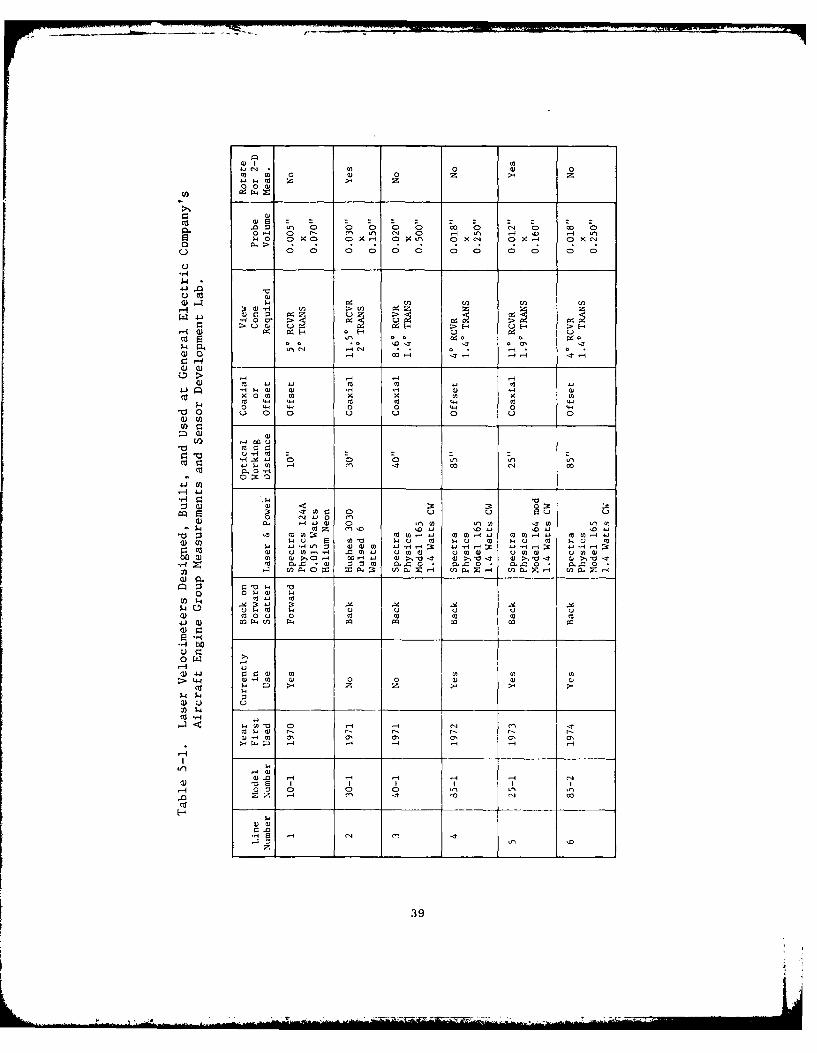
5-1. Laser Velocimeters Designed, Built, and Used at GeneralElectric Company's Aircraft Engine Group Measurements andSensor Development Lab. 39
5-2. Signal Processors Developed by General Electric for Usewith the Laser Velocimeters. 41
7-1. Relationship of Za/2 to 8. 59
7-2. Data Points Required. 60
7-3. Error Percent in Mean Measurement with 95% Confidence as a
Function of N and n. 65
7-4. Fractional Error in Percent for Turbulence Estimate asa Function of N. 66
10-1. Summary of Turbulent Properties Measured on a ConicalNozzle.
10-2. Summary of Turbulent Structure Properties Measured on aCoannular Plug Nozzle. 105
10-3. Summary of In-Jet LV to Far-Field Acoustic Cross-CorrelationMeasurements for a Coannular Plug Nozzle. 113
xi

LIST OF SYMBOLS
a Lens to object-plane distance
a Lens to image-plane distance
ao Ambient speed of sound
A Area ratior
b Beam separation distance
d Diameter of central bright spot (Airy disc)
D Incident beam diameter (Sections 4 and 5); also used as the diameter
of a circular jet
Deq Equivalent Diameter - diameter based on the total area of the nozzleD2 Th aueo 2 Ru 2 p'2
D The value of _ 2 at T that corresponds to Ru 2p' at its maximummax T
e The fractional error in an estimate:
xe =x
E{x} Expected value operation in statistics:
E{x} = f x fx(x)dx
f Lens focal length (Sections 4 and 5); also used as frequency
f(O) Longitudinal turbulence correlation function
f Probability density functionX
F Probability distribution function:x
Fx(X) = x
h Slit width (Sections 4 and 5); annular gap height for a coannular
plug nozzle
I Local intensity in laser beam (Sections 4 and 5); Acoustic intensity
in the far-field
KLength ray vector
xii

I. Length of beam intersection
L Integral turbulence length scale (see Figure 10-5)xth
mn The n central moment of a probability distribution:
mn . f(x - Vx) n fx(x)dx
M Convection Mach number (Vc/ao)c
Mj Ideal jet Mach number
n Number of wavelengths
p Static pressure
p' Acoustic pressure
P Width of slit image (Sections 4 and 5); probability(Sections 7 and 8)
P Pressure ratio (total to ambient)r
r Distance between jet noise source and far-field observer; alsoused as a radial coordinate for nozzle geometry specification
RL The correlation function of an eddy in the Lagrangian frame
R XY(T) The cross-correlation function between random variables x(t) andy(t+T)
R xy(T) An estimate of R xy(T)
R Radius ratior
Total cross-correlation function defined as:R u~2
E{u 2() p'(",';T)} = u 2(y) p'('X,";T)
When discussed as normalized:
2 -u2(') p'(xy;T)
(u2 2 ,2
R Total cross-correlation functionTotal
S Fringe spacing
xiii

S(RTota 1) Spectrum of Ru2p
S.32 foal 22Spectrum of
t Transit time between bright fringes (Sections 5 and 5); time
t Defined as Z except the probability is student T with N degrees offreedom
Tij Lighthill's stress tensor (see rquation 6-3)
TL The total time length of the data record used to estimate acorrelation function
TT Total temperature
u Dimensionless parameter (Sections 4 and 5); Instantaneous velocity
u' Turbulence velocity
U Mean velocity
v Dimensionless parameter (Sections 4 and 5)
VParticle velocity (Sections 4 and 5)
V Ideal jet velocity
V Jet noise source volume element0
VARfx} The statistical variance of the random variable x:
VAR{x} = E {(x - E{x)) 2
= E {x2 - E2 {x}}
V Convection velocityc
Vmi x Specific thrust or weight flow average velocity for a coannularnozzle configuration; or mixed velocity defined as:
(V o+ V i)( + (*)I .
V Velocity component perpendicular to the fringesy
X Distance along cptic axis of lens (Sections 4 and 5); coordinatealong jet axis
xPosition vector from origin to observer
xlv

yPosition vector from origin to jet noise source element
Z The point on the unit Gausian distribution such that the areaunder the distribution is a:
i12a= exp(- x2 ) dx
CL Included angle between laser beams; also see definition of Za
8 Slit half angle of subtention
ij Unity sensor
A Optical path length (Sections 4 and 5); the width of the time gridused to reconstruct the correlation function (Sections 7 and 8)
AV Scattering frequency
a Observation angle
0 Convection amplification factor (see Equation 6-5)
X Wavelength of coherent radiation (Sections 4 and 5); the averagerate of arrival of particles at the probe volume of the laservelocimeter
W(t) The unit step function
(t) = I ; t > o
W(t) = 0 ; t < o
I) (t) The Dirac delta function0
W x The expected value or mean of the random variable x.
The operation distance between LV probe volumes in a two-pointvelocity correlation measurement
P Fluid density
ox The standard deviation of the random variable x; also the turbu-lence level
Time
To The retarded time (r/ao )
Ti The value of T where IR (T)I is maximumxy
xv

T The viscous stress tensor
wf Typical radian frequency of turbulence
Wt Radian frequency in the turbulence
LWeight flow
Super Scripts
i Inner stream of coannular plug nozzle
o Outer stream of coannular plug nozzle
xvi

1.0 SUMMARY
The High Velocity Jet Noise Source Location and Reduction Program (Con-
tract DOT-OS-30034) was conceived to bring analytical and experimental know-
ledge to bear on understanding the fundamentals of jet noise for simple and
complex suppressors.
Task 3, the subject of this report, involved the experimental investi-
gation of suppression principles, including developing an experimental data
base, developing a better understanding of jet noise suppression principles,
and formulating empirical methods for the acoustic design of jet noise sup-
pressors. Acoustic scaling has been experimentally demonstrated, and five
"optimum" nozzles were selected for anechoic, free-jet testing in Task 5.
Volume I - Verification of Suppression Principles and Development of
Suppression Prediction Methods - Some of the experimental studies (reported
in Volume II) involved acquisition of detailed, far-field, acoustic data and
of aerodynamic jet-flow-field data on several baseline and noise-abatement
nozzles. These data were analyzed and used to validate the theoretical jet
noise prediction method of Task 2 (referred to as M*G*B, designating the
authors' initials) and to develop and validate the empirical noise-prediction
method presented herein (referred to as M*S, designating the last name ini-
tials of the authors).*
The Task 2 theoretical studies conclude that four primary mechanisms in-fluence jet noise suppression: fluid shielding, convective amplification,
turbulent mixing, and shock noise. A series of seven suppressor configura-
tions (ranging from geometrically simple to complex) were evaluated in Task 3
to establish the relative importance of each of the four mechanisms. Typical
results of this evaluation of noise mechanisms are summarized in Figure 1-1
in terms of perceived noise level (PNL) directivity for a conical nozzle. In
general, mechanical suppressors exhibit a significant reduction in shock
*The Task 3 empirical (M*S) method was initially intended for nozzle
geometries which could not be modeled in the purely analytical Task 2(M*G*B) method (a multielement nozzle with a treated ejector, forexample).

" M*G*B PredictionsI
" Pressure Ratio =3.28I
" Exhaust Stream Total Temperature =16300 R
Total Without Shock Noise
and Fluid Shielding
Il Total Noise
lo iB
Total Without Shock' Noise, Flui .d Shielding,and convecti m Ification onSock No
Total~Soc Noise hckNos
/4e
.-- S" "----ss. "
20 40 60 80 100 120 140 160Angle to Inlet. degrees
Figure 1-1. Evaluation of Noise Mechanisms for a Conical Nozzle.
2
noise relative to a baseline conical nozzle, reduce the effectiveness of
fluid shielding (increase rather than suppress noise), reduce the effective-
ness of convective amplification (reduce noise), and produce a modest reduc-
tion in turbulent mixing noise. The largest amount of shock noise reduction
correlates with the suppressor which has the smallest characteristic dimension.
Fluid shielding decreases because suppressors cause the mean velocity and
temperature of the jet plume to decay faster than the conical baseline. A
reduction in convection Mach number (and hence in convective amplification)
occurs because a suppressor plume decays very rapidly. Turbulent mixing
noise is reduced through alteration of the mixing process that results from
segmenting the exhaust jet.
Aerodynamic flow-field measurements (mean-velocity profiles) were demon-
strated to be useful in verifying the flow-field predictions which were cal-
culated by the M*G*B (theoretical) noise-prediction program. Noise source
location devices such as the Ellipsoidal Mirror (EM) were demonstrated to be
less useful than the Laser Velocimeter (LV) for the M*G*M theory verification
studies because the LV provides data which may be directly compared with
predictions made using the M*G*M program. Axial and radial mean-velocity
profiles are typical examples of such comparisons.
The empirical M*S jet noise prediction method has been developed to pre-
dict the static acoustic characteristics of multielement suppressors appli-
cable to both advanced turbojets and variable-cycle engines (which are repre-
sentative of power plants for future supersonic cruise aircraft). The effect
of external flow on the M*S jet noise prediction is discussed in the Task 6
Design Guide Report. Inputs required to use the M*S computational procedure
include: element type, element number, suppressor area ratio and radius
ratio, chute-spoke planform and cant angle, and plug diameter. The predic-
tion accuracy is estimated to be +3.3 Effective Perceived Noise Decibels
(EPNdB) at a 95% confidence level. Figure 1-2 illustrates the correlation
between measured and predicted EPNLs for all types of suppressors.
The merits of both the M*S and M*G*B computational techniques can be
stated as follows. The empirical (M*S) jet noise prediction method, based on
correlations of scale-model jet data, serves as a useful preliminary design
3

o Flyover calculation using static data corrected to free-field conditions.
9 The "Reference" level is the predicted value of noise for each nozzle,
at a specified set of thermodynamic conditions, plus an arbitraryvalue of 100 dB.
115 1 1
Nozzle Type 0 1
110 0 Single-Flow, Multitube "
6 Single-Flow, Multichute/Spoke 0
0 Dual-Flow, Multitube __
m 0
U Dual-Flow, Multichute/SpokeZ 105 q -B I
0 0
U90
32r. 100 0__QS.!
a -_.,__
.. [ 0 e90re-Euas-redctd in
W I I0
95I I I
PrdtdEPLR liearo Regerene Confidenc
80ur 1-. o-eato Betee Constedants Lre eldBciePrevd
0 b73 5 80 8 0 09 0 0 1 1
Figre1-2 Crreaton etee Measured-Eqad Predicted Effectv ecie
Noiseostnt Level, PL o l ye fSprso NozB s
4 5

and prediction tool for selecting the basic nozzle type (chute, spoke, multi-
tube, etc.) and primary geometric parameters (element number, area ratio,
etc.) for a given application. It is also useful in evaluating the acoustic
performance of a given suppressor nozzle, provided the nozzle is one of the
types from which the correlation was derived. Further, the method is useful
for doing parametric studies since the computation procedure is relatively
simple and economical of both computer time and cost. The theoretical
(M*G*B) prediction method, on the other hand, is more suited to detailed de-
sign and analysis of a suppressor nozzle. It can supply detailed information
on the jet plume flow development as well as the far-field acoustic character-
istics. It is also capable of evaluating changes in nozzle planform shape,
element placement and spacing, etc. In addition, the theoretical prediction
model is a useful diagnostic tool, capable of assessing the relative roles the
various mechanisms play in the noise suppression process, and can also serve
as a source location analysis tool.
Volume II - Parametric Testing and Source Measurements - A parametric
experimental series was conducted to provide far-field acoustic data on 47
baseline and suppressor nozzle configurations and to provide aerodynamic
nozzle performance on 18 of the configurations. The data presented in this
volume were taken for use in the current program as well as to provide an ex-
tensive, high-quality, data base for future studies. The impact of varying
the area ratio and velocity ratio of dual-flow, baseline nozzle configurations
was investigated, and the importance of shock noise was assessed. The impact
of varying area ratio and element number was parametrically studied for both
single and dual-flow suppressors; core plug geometry, velocity ratio, and
weight flow ratio were evaluated for dual-flow suppressors. These studies
establish absolute static suppression levels on the basis of normalized maxi-
mum PNL, for several families of suppressor nozzles, as illustrated in Fig-
ure 1-3.
Parametric testing identified the following primary trends for single-
flow and for dual-flow suppressors during static operation:
5

i i
Single-Flow NozzlesT_ T_114_
36-Chute Nozzlu withi Acoustically
Treated Ej oA 2.-
12 Je Lr AR 2.0%
1 4 I %
12 0 "36-Chute Nozzle
Shrud A10 AR 2.0 - -1 _
o. - -36-Spoke Nozzle, AR 2.0
6OE 36Cht Nozza Annuppru s Ae) ze FlolAr/ann a
NualFE: NozzloeNsle av uprssr o h
0
Ias Al eag Veo Iv, t/e
Figure ~ ~ Nrb 1-. TyialPakSaticl No ls ae Suppresso actesis
6
Single Flow
0 Suppression increases with increasing area ratio at high jet
velocity.
* Suppression decreases with increasing area ratio at low jet
velocity.
* Suppression level is affected by element type (spoke systemssuppress slightly better than chutes).
Dual Flow
0 Suppression increases with increasing area ratio..
0 Suppression increases with increasing element number at
high jet velocity.
* Suppression level is affected by core plug geometry [by 2to 3 decibels (dB)I.
9 Suppression increases 3 to 4 dB when a treated ejector is
added to a suppressor configuration.
Selective, free-jet tests conducted on eight configurations indicate
that suppression generally decreases in flight. Typical static versus free-
jet results are shown in Table 1-1.
The aerodynamic performance test recorded on 18 of the configurations
at both static and wind-on conditions is also included in this volume. Base
pressure measurements were taken on several of the models in order to deter-
mine base drag (which is thought to be responsible for the poor aerodynamic
performance of most mechanical suppressors in flight). These wind tunnel
tests identified the following primary trends in aerodynamic performance:
" Performance decreases with increasing element number.
" Performance increases with increasing chute depth.
" Performance increases with increasing ratio of inner flow area
to outer flow area.
" Performance is affected by element type (chutes perform better
than spokes because spokes have higher base drag).
7

Table 1-1. Typical Summary of Nozzle Static and ProjectedFlight Peak PNL Suppression Characteristics.
" Suppression Levels are Relative to a ConicalNozzle at Equivalent Flight Conditions
* V = 2500 ft/sec
Suppression Level, db
Configuration Static Flight
Plug Nozzle - 0.789 Radius Ratio 1.3 3.0
Plug Nozzle - 0.85 Radius Ratio 2.3 3.7
8-Lobe Nozzle 5.6 5.6
AR = 2.5 36-Chute Nozzle 13.5 10.9
AR = 2.5 36-Chute Nozzle with AuxiliaryFlow 12.5 9.4
104-Tube Nozzle 12.0 12.0
l8

The base pressure correlations provide a procedure for predicting sup-
pressor nozzle aerodynamic performance.
Volume III - Suppressor Concepts Optimization - Several studies were con-
ducted to attempt an optimization of suppressor concepts. The end product of
this overall effort was to design five nozzles for static and free-jet testing
in Task 5. Trade studies of performance versus suppression, aircraft inte-
gration studies, and development of a figure of merit method of analysis all
make up the activities in this "optimization" process.
Trade studies of suppression versus aerodynamic performance indicate that
a properly selected and designed mechanical suppressor can attain a delta
suppression to delta thrust coefficient ratio (APNL/ACf ) of almost 3.0
(based on static suppression and wind-on aerodynamic performance).
The aircraft integration study consisted of ranking nine baseline and
suppressor nozzles with respect to performance level, suppression level,
weight, impact on aircraft mission range, and noise footprint. In general,
suppression level was found to be the most important design variable, with
performance and weight ranking second and third, respectively.
The appropriate figure of merit, considering all the design variables,
was found to be aircraft range. However, use of range as the figure of merit
requires that the aircraft mission be specified, and several techniques for
cursorily ranking the suppressors based solely on suppression level, perfor-
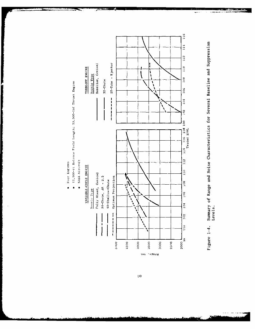
mance, and weight may also be identified. A summary of the range versus noise
characteristics of typical nozzle configurations is presented in Figure 1-4.
Once a noise goal is specified, adding a suppressor provides a significant
range improvement over an unsuppressed system because adding a suppressor is
less costly than reducing noise by enlarging the engine to reduce jet velocity.
The design of the five optimum nozzles was based on data from previous
studies, performed by government and industry, on the M*G*B and M*S models
discussed above and on the parametric data obtained in the acoustic and aero-
dynamic performance test series reported in Volume II. The configurations were
designed and fabricated for open-throat, anechoic, free-jet testing in Task 5.
The configurations chosen for evaluation were: (1) a 32-chute, single-flow
w CL
0
-4
CR 0*- C) I - -
=o C)CC) ~CI
Z C) C) C4-C.) (A
+1-' F- C) Q
c. .4 eq wR C'd
CL-
~CC 0
% % %+
In m N
C)-~ D'C1 0

nozzle; (2) a 40-shallow-chute, dual-flow nozzle; (3 and 4) a 36-chute, dual-
flow nozzle, with and without a treated ejector; and (5) a 54-element, co-
planar-mixer, plug nozzle.
Demonstration of acoustic scaling for several suppressor configurations
was conducted to assure the adequacy of using scale-model results to project
full-scale suppression levels. Full-scale data were obtained on several sup-
pressor configurations using J79 and J85 engines. The suppressors evalua.ed
were: (1) a baseline conical nozzle, (2) a 32-chute nozzle with and without
a treated ejector, (3) an 8-lobe nozzle, and (4) a 104-tube nozzle. Scale-
model data were obtained for these same configurations to allow comparison of
scale-model and full-scale results. In general, peak full-scale suppression
levels projected from scale-model data were verified by the full-scale engine
results. Directivity patterns were duplicated within +2 PNdB (the largest
differences occurring with the conical nozzle configuration). Some spectral
anomalies were observed for select cases; however, they were not of suffici-
ent magnitude to invalidate the scale-model results. The conclusion re-
sulting from this study is that full-scale noise levels can be predicted from
scale-model test results using Strouhal scaling laws.
Volume IV - Laser Velocimeter Time Dependent Cross Correlation Measure-
ments - In-jet/in-jet and in-jet/far-field exhaust noise diagnostic measure-
ments conducted using a Laser Velocimeter (LV) are reported in this volume.
Measurements were performed on a conical nozzle and a coannular plug nozzle.
Two-point, space/time measurements using a two-LV system were completed for
the conical nozzle. Measurements of mean velocity, turbulent velocity, eddy
convection speed, and turbulent length scale were made for a subsonic ambient
jet and for a sonic heated jet. For the coannular plug nozzle, a similar
series of two-point, laser-correlation measurements were performed. In addi-
tion, cross correlations between the laser axial component of turbulence and
a far-field acoustic microphone were performed.
Volumes I, II, III, and IV contain the results of a comprehensive effort
to identify and integrate the theoretical studies, parametric test data,
acoustic and performance diagnostic measurements, and system studies. A
logical procedure has evolved for conducting suppressor design trade-offs.
11

2.0 INTRODUCTION
The first 20 years of commercial aircraft operation with jet propulsion
have clearly demonstrated the need for effective high velocity jet noise
suppression technology in order to meet community acceptance. Aircraft sys-
tem studies show that an efficient jet noise suppression device is required
if a commercial supersonic aircraft is to be economically viable as well as
environmentally acceptable. The current state of the art of high velocity
jet noise suppression would make a supersonic transport (SST), with advanced
technology engines, meet 1969 noise rules (at best). This state of the art
is represented by the material in Reference3 1 through 6.
Reference 1 describes analytical and experimental investigations which
were conducted in the early 1960's. This study established a basis for de-
velopment of mathematical and empirical methods for the predictions of jet-
flow-field, aerodynamic characteristics and for determining the directional
characteristics of jet noise suppressors. This work was limited in the sense
that the suppressors evaluated had only modest suppression potential, and the
measurement techniques available did not allow the acquisition of high-
frequency, spectral data necessary to establish full-scale, PNL suppression
levels.
The development of commercial SST vehicles by the U.S. and by the British-
French multinational corporation in the 1960's placed extreme emphasis on the
need for effective and efficient noise suppression devices. Phase I of work,
conducted by the Boeing and General Electric companies, is summarized in
References 2 and 3. Primary emphasis was on jet noise suppressor development
through model and engine testing applicable to an afterburning turbojet
engine. Suppressor designs were based primarily on empirical methods. Phase
II of this effort, References 4 and 5, continued the suppressor development
with a stronger emphasis placed on the integration of analytical studies and
experimental test data. Specifically, the Boeing Company concentrated on
optimization of tube-type-suppressor systems and related semiempirical pre-
diction methods. General Electric focused on the development both of chute
and of tube-type-suppressor systems with primary emphasis placed on optimiza-
tion of chute-type-suppressor nozzles.
12

Similar studies were conducted by the British and French in development
of the Concorde, and typical results are summarized in Reference 6.
The design technology represented in References 1 through 6 is primarily
semiempirical. The absence of general design rules based on engineering
principles led to the Government's formulation of the High Velocity Jet Noise
Program, Contract DOT-oOS-30034, in 1973. The purpose has been to achieve
fundamental understanding, on a quantitative basis, of the mechanisms of jet
noise generation and suppression and to develop design methods.
This report presents the results of Task 3 of the contract. It provides
the experimental data base which was used in conjunction with the supporting
theories from Task 2 to develop a better understanding of jet noise and jet
noise suppression.
The report is organized into four volumes (FAA-RD-76-79, III - I, II,
III, IV) and is presented in a format consistent with the Task 3 work plan
division of the subtasks. Volume I is entitled "Verification of Suppression
Principles and Development of Suppression Prediction Methods." Volume II is
a data report entitled "Parametric Testing and Source Measurements," and
Volume III is an analysis report entitled "Suppressor Concepts Optimization,"
Volume IV, under this cover, is an analysis report entitled "Laser Velocimeter
Time Dependent Cross Correlation Measurement."
Volume I uses the data base (Volume II) and the Task 2 theoretical model
(Reference 7) to postulate the suppression mechanisms. Volume I also presents
an independent, empirical, static jet-noise-prediction method which was de-
veloped from engineering correlations of tbe test data. Volume II presents
the data and results of the parametric acoustic tests, the aerodynamic per-
formance tests, and the Laser Velocimeter tests. Volume III presents the
results of a trade study of performance versus suppression, an aircraft inte-
gration study, a "figure of merit" methodology, and a summary of the five
"optimum" nozzles selected for testing in Task 5. An acoustic-scaling investi-
gation was conducted to support the suppressor concepts optimization activi-
ties and is presented as an Appendix to Volume III. Volume IV presents the
results of the in-jet/in-jet and in-jet/far-field cross correlation investiga-
tions.
13

The work reported in the present volume describes a number of new laser
velocimeter processor and data handling concepts that are required for real-
time cross-correlation type measurements. Of particular note are discussions
of a filter bank laser velocimeter processor design approach, combined with
the use of a quantized product-factoring computational concept for data
handling that has enabled the successful measurement of two-point, space-time,
cross-correlation measurements in realistic gas flows. A series of laser
velocimeter cross-correlation measurements (using two laser velocimeters) are
reported for a conical nozzle and a coannular plug nozzle at high velocities
(2200 fps) and temperatures (16750@ F) in which the exhaust jet turbulent
length scale and convection speed were measured. Additionally, the laser was
successfully used to determine regions of strong correlation between the
velocity field and the acoustic far-field pressure for a coannular plug noz-
zle. These recent results indicate that the technology is now available for
performing systematic and detailed jet noise source location diagnostic
studies for jet nozzles operating at realistic velocity and temperature condi-
tions.
14
3.0 GENERAL REMARKS ABOUT THIS REPORT
During the course of the last several years the General Electric Company
has been engaged in a number of theoretical and experimental investigations
aimed at developing a better understanding and quantification of jet exhaust
noise of simple circular nozzles and complex mechanical type exhaust nozzle
suppressors. The support for this work has come from a number of Government
agencies (FAA/DOT, Air Force, and NASA) as well as from General Electric
research and development funds. Both scientists and engineers at the General
Electric Company, as well as engineers at a number of other industrial insti-
tutions, universities, research laboratories, and Government research centers
have exerted and shared considerable time, talent and experience to solve and
mitigate the aeroacoustic aspects of high-velocity and temperature exhaust-
jet noise.
Typically, one-millionth of the total jet flow power is radiated as
acoustic power, hence the difficulty to quantify and reduce jet noise.
Realistic exhaust jets operate at high velocity and temperature. Therefore,
complex and precise measurement and test facilities are required. The jet
noise producing agents are aerodynamic in nature, and are airborne - hence
rugged, but sensitive real-time aerodynamic and acoustic measurements of
micro scale jet aerodynamic properties are necessary. Underscoring these
problems is the fact that theoreticians are still probing for the most exact
or best theoretical acoustic formulations for jet noise generation and for
acceptable approximations for their solution. Considerable progress has been
made in acoustic testing, theoretical acoustic modeling and engineering
design procedures such as that reported in the various task reports under
this program (Report Series FAA-RD-76-79).
One perplexing task in verifying the "exact" nature of jet noise genera-
tion is to develop the proper measurement tools, particularly those associ-
ated with measuring the aerodynamic real-time flow properties. This report
discusses work carried out by the General Electric Company to develop a real-
time velocity measurement system, the laser velocimeter.
15

Section 4.0 of this report contains descriptions and discussions of the
fundamentals of laser velocimetry, and its unique problems. Section 5.0
contains an up-to-date description of General Electric's laser velocimeter
system, including some unique real-time velocity processing features cur-
rently not available in the open literature. The theoretical aeroacoustic
motivation for performing real-time velocity measurements is discussed in
Section 6.0, where a perspective Is given for performing real-time, two-
point, space-time measurements for the purpose of measuring jet global
turbulent structure properties, and for setting a frame work for noise source
location studies. Sections 7.0 and 8.0 contain the theoretical statistical
considerations necessary for performing real-time velocity measurements and
cross-correlations with the discontinuous output of the laser velocimeter.
Particular attention is devoted in these sections to define the concepts
developed at GE which successfully permitted accurate measurement of mean and
turbulent velocities, turbulent spectra, and two-point space-time cross-
correlation measurements with two lasers, or with one laser and an acoustic
microphone. The concepts discussed in Sections 7.0 and 8.0 will provide a
basis for future investigators to assemble the type of computational algorithms
necessary for processing real-time data samples in an economic fashion.
Section 9.0 describes the laser velocimeter test arrangement used in performing
many of the reported advanced LV diagnostic measurements. Section 10.0
contains the results of a number of key LV jet plume studies, including:
discussions of some high lights of mean and turbulent velocity measurements
performed on high velocity and temperature shocked and shock free conic
nozzle flows, LV measured turbulence spectra, a comprehensive series of two-
point space-time measurements on a conic nozzle and an inverted flow coannular
plug nozzle for turbulent length scale and convection velocity, and a series of
LV to farfield acoustic cross-correlation measurements on a coannular plug
nozzle. The emphasis of all experiments was to illustrate the capability for
performing diagnostic type velocity measurements in realistic high velocity
(supersonic) high temperature nozzle flows. The measurements reported are
believed to be unique and important for future investigations of this kind.
Section 11.0 contains a summary and recommendations for future work in uti-
lizing the laser velocimeter for jet noise diagnostics.
AL'i

4.0 THE LASER VELOCIMETER AND APPLICATIONS TO JET NOISE DIAGNOSTICS
This section reviews the need for and the fundamentals of laser veloci-
metry, the historic background of the technique, and unique problems and solu-
tions in the application of laser velocimetry to jet noise diagnostics.
4.1 THE NEED FOR A NON-INTRUSIVE DIAGNOSTIC METHOD
Historically, in diagnostics of ambient, subsonic jets, a variety of
instrumentation has been available which creates relatively little disturbance
on the local or global jet properties. Thus, miniature pitot-static probes,
very small, streamlined microphones, hot wire anemometers, etc. were adequate.
Such has not been the case for a hot, supersonic jet. Various non-disturbing
techniques using optical effects such as Schlieren photography, holography,
correlated two-beam refraction and laser velocimetry have been attempted by
industrial and educational researchers throughout the world. Ten years of
experience has shown that the most viable diagnostic techniques must be accu-
rate and highly localized. This accounts for the outstanding acceptance of
laser velocimetry.
4.2 HISTORICAL SKETCH OF LASER VELOCIMETRY
The concept of measuring the velocity of a gas flow by the Doppler shift
of light has been known for a number of years. In 1948, Hessrs, Bundy and
Strong of the General Electric Research and Development Center published a
report(8 ) on the measurement of gas velocity in a rocket exhaust, using the
Doppler shift of light emitted by a trace of vapor of an alkali metal seeded
in the flame. The concept, however, was limited to velocity measurements of
hot gases where thermal excitation is sufficient to cause the alkali metal
seeding material to radiate at its resonance spectral line. In the 1960's,
the invention of the laser provided a light source with enough output and
coherence to make heterodyning techniques feasible. In 1964, Yeh and Cummins
also published material on this subject (9 ) . However, improvements in utility
and arrangement were needed. In 1969, a particular arrangement of the laser-
powered Doppler technique, called "Differential Doppler" was first described
i7

by C.M. Penney of the General Electric Co. Research and Development Cen-(10)
ter " The geometry of this arrangement is such that measurements of fluid
flow velocities can be made in situations where there is access at only one
side of a stream. Further, the differential Doppler arrangement is easy to
align and calibrate. Today the vast majority of users, worldwide, are employ-
ing the Differential Doppler method, rather than the original reference beam
arrangement.
4.3 FUNDAMENTALS OF LASER VELOCIMETRY
The laser velocimeter is a noncontact air-speed-measuring instrument which
consists of a laser, seed particles, mirrors, lenses and beamsplitters, a
photodetector and a signal processor. Figure 4-1 is a schematic view of the
basic differential Doppler arrangement. The laser beam is split into two
equal power beams that are focused and crossed in space, where the air speed
is to be measured. Interference "fringes" are formed here (they can be seen
with a microscope and some smoke). The fringes are plane, parallel, light
and dark sheets that, on edge, resemble a picket fence. A single dust particle
(seed) passing through this region scatters light in a sinusoidal burst,
detected by a phototube. This is analogous to running alongside a picket
fence, rapping it with a stick. The frequency of the sine burst is measured
by a signal processor. Figure 4-2 is a simplified schematic diagram of the
measuring process. A "counter-timer" is shown here, but there are other
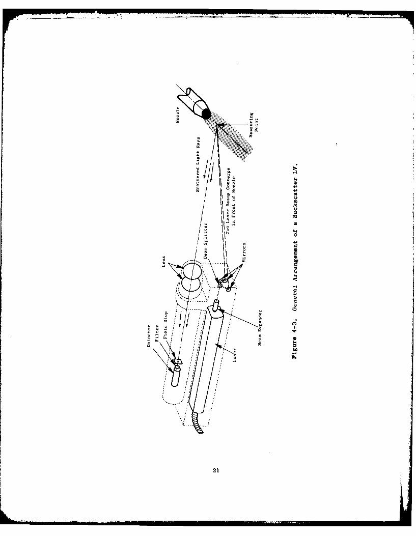
techniques. Figure 4-3 is a cross section to show how the basic components
might be arranged for a single component, back-scatter system. Back-scatter
means that only a small amount of the particle's scattered light is collected,
and in the back direction.
4.3.1 The Differential Doppler Method
The LV technique can take the form of one of two optical configurations:
reference-scatter (direct Doppler), Figure 4-4; or differential Doppler (dual
scatter), Figure 4-5). The ease of alignment and usage plus the inherent
increase in a signal-to-noise ratio have made the differential Doppler con-
figuration predominant in the literature and the method chosen by General
Electric.
1is

lo AL
- 0oM
0-
4A VI w
0
-r4
04
ZU00)
00I-
0 I
I--
I .4
/ ~L9

z
-A0
-4 4-
41 Q)
C>
U-4 0Z bbl
Cd T-U)414z0
bL -
'0-
414
r4 -
(-. r- U
C) U)-404 0
rz) C."0
44 C
CC)
200
-At
Q? 0.
00
u' 0.4J
10 CH
0
I. I40
0 0t
212

Photo TLubeIt
Beam Splitter (
, )I
Scattering VolIume
Be am LT ro
Neutral Density
Filter
Figure 4-4. Reference-Scatter or Direct Doppler Arrangement.
L z--ScatteringMiro 00 t! Volume L c
K022
Laer Q7 K PhotoBea --nKO Tube
BeamSplitter
Figure 4-5. Dual-Scatter or Differential Doppler Arrangement.
22
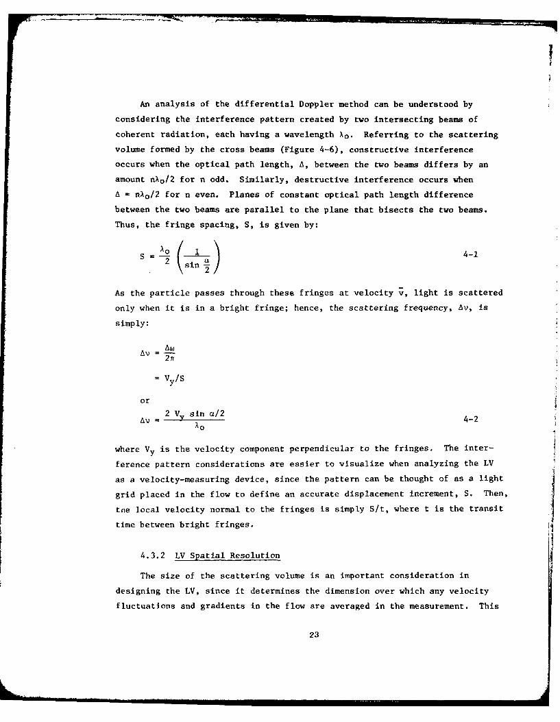
An analysis of the differential Doppler method can be understood by
considering the interference pattern created by two intersecting beams of
coherent radiation, each having a wavelength Xo. Referring to the scattering
volume formed by the cross beams (Figure 4-6), constructive interference
occurs when the optical path length, A, between the two beams differs by an
amount nXo/2 for n odd. Similarly, destructive interference occurs when
A = nAo/2 for n even. Planes of constant optical path length difference
between the two beams are parallel to the plane that bisects the two beams.
Thus, the fringe spacing, S, is given by:
s A 4-12 - sina
As the particle passes through these fringes at velocity v, light is scattered
only when it is in a bright fringe; hence, the scattering frequency, Av, is
simply:
A A27r
= V /Sy
or
2 V sin a/2 4-2Av=4-
Ao
where Vy is the velocity component perpendicular to the fringes. The inter-
ference pattern considerations are easier to visualize when analyzing the LV
as a velocity-measuring device, since the pattern can be thought of as a light
grid placed in the flow to define an accurate displacement increment, S. Then,tne local velocity normal to the fringes is simply S/t, where t is the transit
time between bright fringes.
4.3.2 LV Spatial Resolution
The size of the scattering volume is an important consideration in
designing the LV, since it determines the dimension over which any velocity
fluctuations and gradients in the flow are averaged in the measurement. This
23

0 u
N 0'
>: 4< => '-'-
m4 04 4O Ec mI$4u U- 4-4
v 0
.44
~4O 4- ~ 0
cc 0
0 4$
$4
CV-
00
pa0
244
volume is determined by the optics of the transmitter and the collector lenses
and by the size of the laser beam. In most LV arrangements, the beams are
focused to spots in order to minimize the scattering volume. Under these
conditions, the spot size is then determined by the diffraction limit of the
focusing lens.
Consider a beam of parallel, monochromatic light of wavelength A with
uniform intensity, passing through a lens of focal length f. At the focal
point of the lens, a diffraction pattern is formed, and the diameter, d, of
the central bright spot (called the Airy disc) is given (11) by the relation-
ship:
d = 1.22 Xf/D 4-3
where D is the incident beam diameter. This same diffraction limit in the
size of the spot at the focus of the transmitter lens determines the scatter-
ing volume with a laser beam.
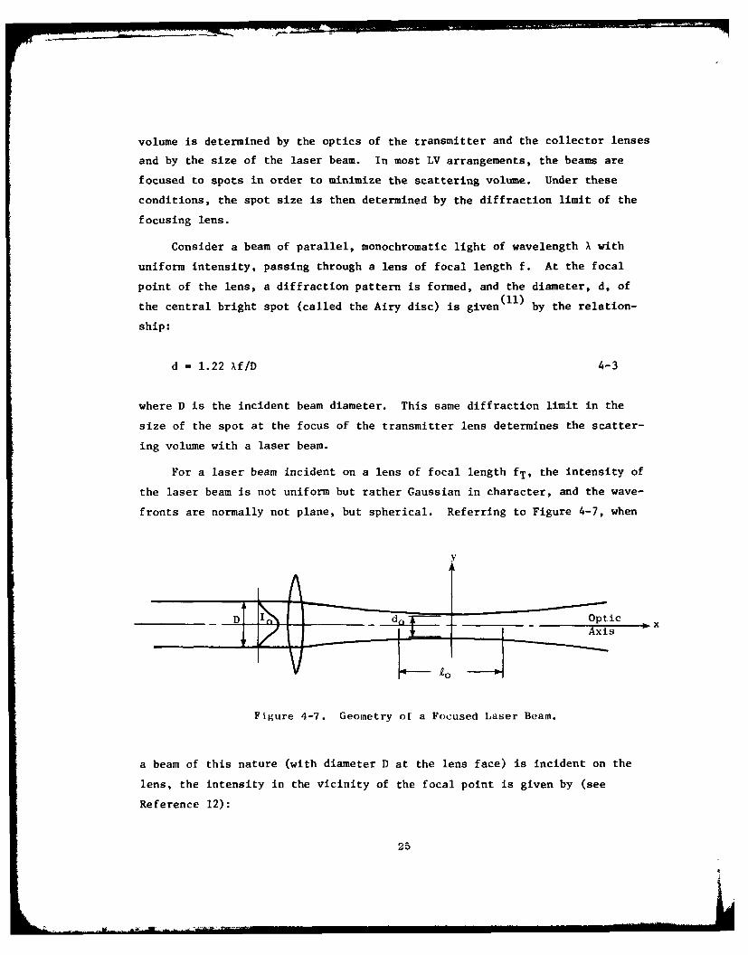
For a laser beam incident on a lens of focal length fT, the intensity of
the laser beam is not uniform but rather Gaussian in character, and the wave-
fronts are normally not plane, but spherical. Referring to Figure 4-7, when
D _do_----- " Optic
Axis
Figure 4-7. Geometry of a Focused Laser Beam.
a beam of this nature (with diameter D at the lens face) is incident on the
lens, the intensity in the vicinity of the focal point is given by (see
Reference 12):
25

II
I(uv)= 0 e-v2/(l + u2); 4-4W(1 + u
2
where
Trx D2
2 f2
v TryDXfT
and y and x are coordinates measured perpendicular to and along the optical
axis of the beam, respectively, with origin at the focal point of the lens.
Thus, the focused beam is seen to be a distorted ellipsoid of revolution with
the intensity falling off sharply as a function of x and y. For the intensity
to drop to one percent of its incident value, Io, the size of the spot is:
do = 1.184 XfT/D and 4-5a
to = 7.08 X(fT/D) 2. 4-5b
These two equations give the relative dimensions of the full scattering volume
without the use of apertures and stops in the collector optics.
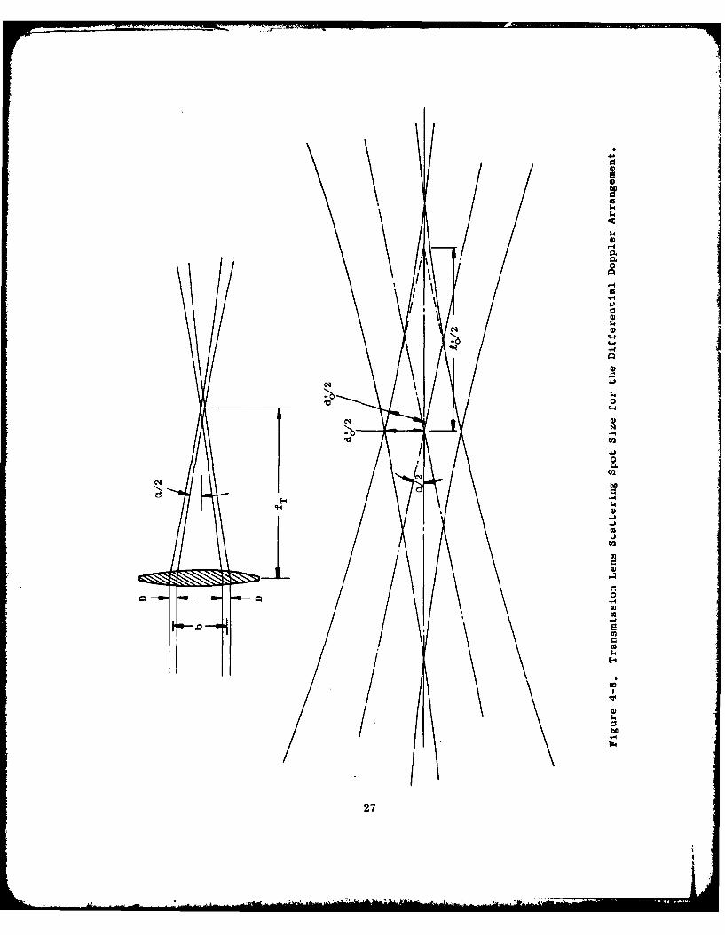
For the differential Doppler method, the two beams intersect at the focal
point of the transmitter lens, and the interference fringes are formed only
where the beam intersect. Referring to Figure 4-8, when the two beams (of
diameter D separated by a distance, b, are focused by the transmitter lens,
the width of the spot do' is:
d'- 4-60 cos (a/2)
where a is the angle between the beams, and do is calculated by Equation 4-5a.
Similarly, neglecting the beam divergence in the vicinity of the focal point,
the length of the intersection, ko, is:
26
41.4
$40
eq~
02
C4')
CH $41 .0
4 1
cc
m
-- J L
272

do4 -
sin (a/2)
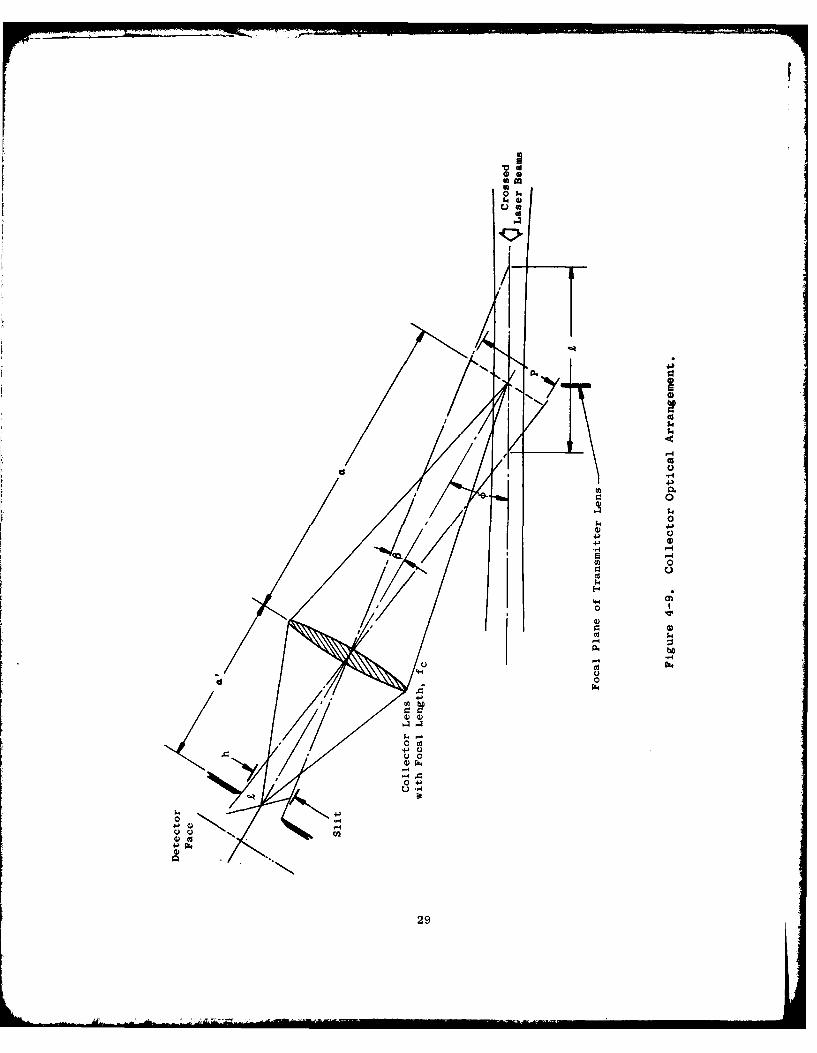
As previously mentioned, stops and apertures in the collector optics are
normally used to limit the size of the scattering volume to a "data probe
volume," since, generally, the dimension of the scattering volume along the
optical axis, ko or V, is too long for good spatial resolution in the flow.
A simple means for reducing this dimension by using the collector optics is
shown in Figure 4-9, where a narrow slit of height h is placed in the image
plane of the collector lens with focal length fc. With this arrangement, the
length of the data probe volume, Z, in the focus of the transmitting lens that
is seen by a detector placed behind the slit is:
sin '
where, p is shown in Figure 4-9, and 4 is the main scattering angle. By use
of the lens formula, one can obtain:
k 2 (a/fc - 1) h/sin 4). 4-8
Thus, the length of the scattering volume can be controlled by a judicious
choice of the collector optics and the scattering angle.
With respect to limiting spatial resolution, it is possible to further
reduce the length of the data probe volume by discriminating the amplitude of
the scattered light. Only when the seed particle passes the middle of the
scattering volume is the incident light (and therefore the scattered light)
at a maximum. On either side of this point, the peak signature amplitude
decreases. Furthermore, at either end of the intersection volume the signa-
ture becomes dual-peaked, which can be responsible for Doppler dropout where
"missing" electronically undiscriminated pulses will improperly add to the
average Doppler period. Thus, by amplitude window thresholding (for particles
of uniform size) and use of a dropout monitor, the spatial resolution can be
increased beyond that generated by the collector optics.
28
4) 0Am
O~4J840
4J
QM -4
/C $4
a C)
44.
4$0 C0
144
' -4o .4=U 0,
(a)
29)
To summarize, the spatial resolution of the IV is determined by both the
transmitter and the collector optics as well as by the use of IV signal pro-
cessor monitors. The width of the spot is normally specified by the diffrac-
tion limit of the transmitter lens and is given by Equation 4-5 or 4-6. The
spot length is determined by the collector optics containing appropriate
apertures and stops to limit the region over which scattered light is collected.
Dropout and amplitude threshold windows also can be provided as signal moni-
tors to further reduce the data volume.
4.4 UNIQUE REQUIREMENTS, PROBLEMS AND SOLUTIONS IN THE APPLICATIONOF LASER VELOCIMETRY TO JET NOISE DIAGNOSTICS
The laser velocimeter (LV) is used for the purpose of accurately sampling
the time history of gas velocity at known points in the nozzle exhaust plumes,
and in a known direction. This sequence of velocity samples can be correlated
to near-simultaneous samples of velocity at some other plume location, and
can also be correlated with near and far-field sound pressure level measure-
ments.
Because these diagnostic LV data must have sample time preserved as well
as represent instantaneous and localized velocity vector components, unique
requirements are placed on the LV system. Added constraints and problems
result when the LV system is expected to work in the non-ideal environment of
heated supersonic jet exhausts. The noise level and temperature extremes in
the vicinity of an exhaust nozzle (model scale or engine size) may seem incom-
patible with a precision, laser powered, optical device. This section will
attempt to prove the contrary, that each of the application problems, when
isolated and fully understood, can be controlled. Thus, the discussion will
include: particles as flow tracers, use of laser light, control volume size
and optical working distance, signal processing choices, angular acceptance in
turbulent flow, and noise and other interfering effects.
4.4.1 The Particle as a Tracer
The clean exhaust jet will not generally scatter the laser light effi-
ciently. An external source is usually required to add tracer particles
to the gas. Several constraints are plaed on these tracer particles:

r.
1. must be small in size (one micron or less) to avoid "slip" errorsin high acceleration fields
2. must be a good light scatterer
3. must survive 2,0000 R
4. must be easily dispersed in gas stream
4.4.2 Laser Light Requirements
The light source must be a laser of high angular and temporal stability.
A complex set of tradeoffs must be made to determine laser power required.
The following parameters or sub-groups of parameters are involved:
1. laser wavelength
2. laser coherence
3. laser beam focusing optics
4. particle size, shape, and scattering optical properties
5. scattering angle selected
6. receiver collector solid angle
7. photodetector quantum efficiency, frequency response and noiseproperties
8. signal processor bandwidth and noise properties
4.4.3 Control Volume Size and Optical Working Distance
The control volume generally is an ellipsoidal shaped volume, whose
dimensions are controlled by choices in the optics (see Section 4.3.2, par-
ticularly equations 4-5 and 4-6). The optical working distance is very
important in jet plume mapping, as it is important to sample the plume with-
out exposing the LV head to the jet blast itself. Thus the working distance
selected will depend on the plume width. The control-volume selected will be
based on expected velocity gradients (primarily that found in the small tur-
bulent eddies in the early mixing region of the plume). A tradeoff exists
here, because a very small control volume well suited to small eddy mapping
may lead to refraction problems. (This is discussed under noise and other
interfering effects.)
31
4.4.4 Types of LV Signal Processors
Various types of LV signal processors may be assessed for their measure-
ment capabilities of the local fluid velocity by deducing the Doppler frequency
of scattered light from a seed particle moving at the fluid velocity. These
signal processing designs include the following major concepts:
1. Spectrum analyzer
2. Doppler frequency tracker
3. Counter-timer
4. Photon correlator
5. Filter bank
Early in the history of the LV, workers used a spectrum analyzer for
processing of the LV signal. Such analyzers, as were and are now available
in well equipped labs, employ a slow frequency scanning principle. This is
equivalent to turning a narrow band receiver across a frequency range. This
type of processor is unsuitable for measuring time dependent flow properties.
An alternative approach to the scanning spectrum analyzer is to digitally
record each Doppler burst, and, at some later time, analyze on a digital
computer. Such a technique was demonstrated by Asher, Scott and Wang(13 )
Advances in microcomputers will soon make on-line analysis feasible and cost
effective.
4.4.4.1 Doppler Frequency Trackers
Doppler frequency trackers have been in widespread use since the late
1960's .0 '14 '15 . Commercial equipment is available, for example, from TSI,
Inc. (1 6 ) and DISA, Inc.( 1 7) Trackers operate by attempting to match the
frequency and phase of an internal, controllable oscillator to the incoming
Doppler burst. A critical parameter in all trackers is the capture range.
Successful tracking can take place only when the incoming Doppler burst fre-
quency is within a certain ratio of the previous burst frequency. This ratio
is called the capture range. Usually this range is 0.9 to I.i. Low seeding
density and high turbulence in a mixing jet can cause successive bursts to
differ by ratios of 0.3 to 3.0. Consequently, the tracker is generally not
usable in jet noise diagnostics.
32

4.4.4.2 Counter-timer
Counter-timer signal processors use conceptually simple principles, but
have features well suited to LV measurements in high turbulence gas flow. The(18)
earliest presentation of the concept was by W.B. Jones . Figure 4-2 is a
simplified diagram of Jones' arrangement. The high frequency, brief burst
from the photomultiplier tube is high pass filtered to remove the gaussion,
low frequency envelope (sometimes referred to as a "pedestal"). The signal
is then amplified and clipped and enters the preset counter which outputs a
single pulse of duration Nt, where t is the burst period and N is the preset
number of cycles to be counted. The pulse enters a width to height converter
that has output Kt as an amplitude. Thus Kt is proportioned to the transit
time of the seed particle through the N fringes. The transit time signal,
Kt, may be recorded, or applied to a display oscilloscope, or both.
The counter-timer processor is widely used in low speed/density flow
where high precision is needed in the measurement. Advanced developments
relating to jet noise diagnostics are described in Section 3.0.
4.4.4.3 Photon Correlation
Photon correlation methods and their application to laser light scatter-(19) (20)ing techniques have been discussed by Pike and by Kalb . The basis of
this approach is the detection of individual quanta of light energy (photons)
recorded in fixed time intervals. Using appropriate digital processing, the
recorded photon "counts" can be shown to represent the autocorrelation func-
tion. This signal then contains time-averaged velocity and turbulence inten-
sity information. For this reason, a photon signal processor could only be
used in a very inefficient way in jet plume diagnostic velocity measurements.
It has been calculated that a velocity spectral analysis using photon correla-
tion would require data collection times in excess of that needed by the
counter-timer, for example, by a factor in excess of 100.
4.4.4.4 Filter Bank
Filter bank signal processing for the LV was first reported in 1968 by
Rolfe et al. (14) Although showing feasibility of using a set of overlapping
3:3

bandpass filters for an efficient spectral analysis, the arrangement was
limited in useiulness. The arrangement averaged many Doppler bursts, finally
yielding mean velocity and turbulent intensity. Times of arrival of individual
bursts were not preserved. The potential for individual burst processing,
however, was later pursued at General Electric, and a filter bank processor
that is suitable for jet plume time dependent measurements was developed and
applied as described in Section 5.0.
4.4.4.5 Summary
The counter-timer and the filter bank were selected by GE to process a
velocity sample from just one particle traverse of the LV control volume.
The spectrum analyzer, Doppler frequency tracker, and photon correlator were
found to be either not capable of or inefficient in handling single particle
Doppler burst data.
4.4.5 Angular Acceptance in Turbulent Flow
As the flow turbulence increases, the velocity components show increas-
ing fluctuations. The signal processor must contend with the wide frequency
range inherent in this process. In addition, turbulence brings about angular
trajectory fluctuations about the jet centerline axis. This illustrated in
Figure 4-10, tracer particle trajectories in the control volume. Three
illustrative particle trajectories of -60', 0', and +600 are shown, where 00
represents the jet axis. Sixteen (16) fringes were placed in the control
volitme in this example. The 0' particle crosses all 16 fringes, but only 8
fringes are crossed by the -60* and +60' particles. The governing equation
of the number of fringes crossed or the prcbe control volume center is a
cosine law, and is illustrated in Figure 4-11. As an example of the signal
processing limits, suppose a control volume of only ten (10) fringes was
used, and the signal processor required eight (8) good cycles (fringes) of
burst signal. In Figure 4-11, the dashed line marked "A" would represent
the angular limit line for this case, where only 0.8 of the total fringes are
crossed. It may be seen that line A intersects the cosine curve at approxi-
mately 37. Thus, particles beyond ±37' would not be measurable. If it was
determined that the angular acceptance of ±37' was not sufficient, then the
34

00
-600 +60*
Figure 4-10. Particle Trajectories in Control Volume.
1.0
SO 0.8-
0.
0
Cd
0 10 20 30 40 50 60 70 80 90Angular Trajectory, degrees
Figure 4-11. Fringes Crossed Vs. Angle of Particle.
35

ratio of processor cycles required over total fringes in the control
volume would have to be decreased. For example, line "B" in Figure 4-11
shows a ±600 angular acceptance when 1/2 of the fringes are crossed.
The examples given are simplified somewhat, in that some particle tra-
verses through the control volume will be off-center and cross fewer fringes
than illustrated above.
4.4.6 Noise and Other Interferring Effects
This section outlines the problems of: optical and electrical noise,
interference from background light, smoke interference, optical refraction,
and environmental protection.
4.4.6.1 Optical and Electrical Noise
Optical and Electrical Noise stems from several sources: A small par-
ticle of non-spherical shape may rotate as it passes through the LV control(21)
volume, creating intensity modulation in the scattered light collected
The focused and crossed laser beams do not have a perfect sinusoidal light
distribution, but have what may be thought of as secondary interference pat-(12)terns . The photosensor exhibits "shot noise" that stems from the very
nature of light: light travels in packets, called photons, that vary in a
statistically predictable and sometimes annoying manner - even from a so-called(22)
steady light source . The impact of these noise sources is, with a single
particle in the control volume, a range of 10 to 30 dB signal to noise ratio
on the Doppler burst itself.
The most influential parameter is the scattered light power incident on
the photo-detector. Any method used to increase the detected light power
will improve the signal to noise ratio.
4.4.6.2 Interference from Background Light
Light received from any source other than the scattered laser light from
the particle constitutes an interference source. Therefore, hot particle
incandescence, illuminated background from roomlight, sunlight, and even the
36

laser beams, may degrade the signal. The laser line filter will remove over
99% of unwanted broadband sources. The filter will not remove background
laser light. This light may only be excluded by keeping surfaces out of the
control volume during data acquisition.
4.4.6.3 Smoke Interference
Smoke interference is related to the background light problem. The
laser light scattered from a heavy concentration of smoke particles presents
the same interference as a surface in the control volume. In addition, smoke
between the control volume and the LV head may attenuate the signal by absorp-
tion and scattering.
4.4.6.4 Optical Refraction
Optical refraction is the bending of light rays in the air space between
the LV head and the jet, and within the jet. Temperature gradients outside
and within the jet plume and static pressure variations within the plume
create the optical index gradients which, in turn, cause the refraction.
Under severe refraction, the laser beams uncross. The loss of the interference
fringes during the uncrossed condition stops the data. Partially uncrossed
beams result in shortened Doppler bursts and/or reduced signal strength.
The immersion depth of the optical path in the hot jet affects the amount of
refraction.
4.4.6.5 Environmental Protection
Environmental protection of the LV head involves several areas. The
mechanical mountings of the laser, mirrors, lenses and receiver optics must
be designed to withstand temperature changes without undue strain. Use of
alloys of equal thermal expansion coefficient, and high thermal conductivity
reduce the strain problem. Acoustic noise and vibration effects can be con-
trolled by designing for the highest possible resonant frequency in the LV
head and internal optics mountings. Smoke and dust must be prevented from
depositing on the optics. Near-air-tight construction, to reduce "breath-
ing", helps. Positive purge with a filtered air source is even better.
37

5.0 DESCRIPTION OF GENERAL ELECTRIC'S LASER VELOCIMETER
This section presents an up-date on the development and status of General
Electric's current arrangement of the real-time diagnostic laser velocimeter
systems. The topics covered are:
" Laser velocimeter optical head
" Signal processors
* Seeding arrangements
" Data acquisition and reduction
5.1 LASER VELOCIMETER OPTICAL HEAD
Since 1970, six LV heads have been designed, built and used. Four are cur-
rently in use. Table 5-1 summarizes the characteristics of these LV heads.
All are of the single component, differential Doppler arrangement (defined in
Section 4.0). All except the Model 10-1 are of the backscatter arrangement.
The optical working distance varies from 10 inches to 85 inches. The shorter
distances are suitable for probing turbomachinery blading. The longer optical
working distances have been designed for probing jet exhaust plumes, where no
physical part of the head is allowed to contact the high speed exhaust jet.
In Table 5-1, the column "Coaxial or Offset" refers to whether the laser
beam's bisector has been arranged to be centered inside of the received
cone of scattered light ("coaxial") or outside of this cone ("offset").
Note also that view cone requirements vary, and probe volume dimensions are
quite different.
The two LV heads used in the cross-correlation measurements (discussed
in Section 10.0) are the models 85-1 and 85-2, lines 4 and 6 on Table 5-1.
Although outside case dimensions are slightly different, the probe volumes
were matched as closely as possible. In two-point velocity correlations,
one LV is operated on the 514.5 nm argon-ion laser "green" line. The other
head is operated on the 488 nm "blue" line. Each photomultiplier tube is
filtered with the appropriate laser line filter. Because of the two colors
38
Q)I U)*U0 Q) 0
Ul m 0 0) 0 zz
0W)
J3 0 0 0 0 0 0 00 0 C1 0 00 00 -4 0 en In~ C1 N 0 -4 L -4 sO -4)4 0 Ox 0x. xXU OX' x~-0o o.>99 9 9 9 9 9
()0 0 0 0) 0 0 0 0 0) 0 0 0)
U)4)U)U
u cc
w ~ o.4C W *n on En-4-> En c4 z .- .- 4
o > g- 4-
U 4 Z-" F-' U o DUo
o ~ ~ ~ -o- 0 0 00. -
af) co4fl
-0 0 0 0 14 0) .4
4-~U -4 r ) In U)
0*0-
i -tW 0 0nL )wu v-)
a. It 4.O 0n :3: a U)U c q c -AW ca E
4C) )U l-. U 34.o U CO.C U4Q cU 4 Q)-~ wUO IjU 4jU UUH UU H :2
It O.X ;d : *U ca 9. a0 4* C aO * (a. j-0 o
ca 0 U u 1 c ac
>443 Oj- O ) a) w)
a) z u
cd -H
- 4 -4 '-4 1-4 -4 N4
4 -4 -, 4 -4 U
*,T4 oo N1 .4
39

used, probe volumes can be moved in close proximity to one another, even
overlapping, without interference. The general arrangement of the 85-1 and
85-2 LV heads are shown in Figure 4-3. The argon-ion laser supports a
3X beam expanding telescope. One beamsplitter and three mirrors are used
to form the two equal power laser beams of about 0.7 watts each. The beam
expander is adjusted so as to focus the laser beams about 90 inches away,
to a spot diameter of 0.018 inches. No other lenses or optics are used in
the transmitter side of the LV. On the receiver side, a pair of symmetrical,
6-in. diameter, acromatic lenses are used to collect a 40 cone of scattered
light and focus through a field stop to the filter and detector. The detector
used is a photomultiplier tube, 0.75 inch diameter "S-20" cathode and potted
dynode resistors. A wideband preamplifier is located about 10 inches from the
detector. Frequency response of the preamplifier is 1 kHz to 150 MHz + 1 db.
Voltage gain is 10OX. Peak output is ± 1 volt into a 50 0 transmission line
(such as type RG8 cable).
The LV box construction is 1/2 inch thick aircraft aluminum alloy sheet,
with a 1/16 inch thick plumber's lead sheet bonded to the inside. The alumi-
num alloy provides a high mechanical resonant frequency and high thermal
conductivity. The lead sheet provides a high mechanical damping. For opera-
tion in proximity to scale model exhaust, no additional acoustic protection
was found to be necessary.*
5.2 SIGNAL PROCESSORS
Since 1970, six signal processors have been designed, built and used,
encompassing five designs. Four are currently in use. Table 5-2 summarizes
the characteristics of these processors. The first four lines of the table
are models based on the counter-timer technique. The fifth line describes
the Mark III signal processor, based on the filter tank technique. A com-
parative description of these techniques is given in Section 4.0.
* The LV has been used in diagnostic testing of a J79 engine at full and
partial power. During such testing a time delay relay tube in the laserpowersupply box (about two feet from the LV head) was broken. Wrapping alead-vinyl acoustic blanket around the laser supply box solved thisproblem and no further damage to the LV was experienced during engine testing.
40

(I)0 0
w ~- 0
w 000 '0 '0 0 O~0
0 .0 -i-I Co -~t~ Lt
CCC CC000-2 0.'
C- '*I-4
-4I---, 2, "0
0) 2,2, '00
-~ 00 ~--~
'-'C OCS *- 0-0 .~-"C
0)CI,
2 ~
(a
cJ
I,) I
CO
0)
*0) K +..0 K
K0) ..- -
o -- --- ---s-0)
<-2
- I
CI,0)00
-4
CO
Cd,
C04
-4-o
CO0) ___ __ 1 __ __ __
A
41

To the counter-timer basic arrangement (line 1, Table 5-2) Mossey
added a wide frequency range pedestal remover (line 2), a precision counter-
timer-comparator (line 3) and a period-to-velocity converter (see Chapter 5
of Reference 23, and Reference 24). This formed the basis of the Mark I signal
processor. Additional refinements were added by Asher (25). The success
of the Mark I processor paved the way to development of the more elaborate
Mark II processor (line 4). The Mark II processor has an advanced check
system. Two of this type of processor are currently in use. The significant
advantage of the Mark II is the greatly reduced error rate in the data out-
put stream over any previous processor.
Because of these discretionary features built into the Mark II signal
processor, the data output rate drops as the signal to noise ratio (S/N) falls
below about 20 db. In order to improve the data output rate under specific
low S/N conditions, General Electric developed the Mark III, a completely
different type of signal processor, shown on line 5 of Table 5-2.
Both the Mark II and Mark III signal processors have been used in diag-
nostic and cross-correlation velocity measurements. A detailed operation
description of each processor is given below.
5.2.1 Mark II LV Signal Processor
The Mark II LV signal processor is illustrated in Figure 5-1. The
amplified Doppler burst signal is applied to the wideband pedestal remover.
The square-wave like output is illustrated in Figure 5-1. This output is
applied to a four stage binary counter, and also to an under-frequency tester.
The binary counter feeds eleven (11) decoders, and each decoder has a unique
logical function. Each decoder feeds a time-to-amplitude converter. The
first nine (9) decoders are for specific single cycles within the burst.
All of these decoders, through their respective time-to-amplitude converters,
feed the all-cycle comparator test. In this test, one of the cycle periods
is chosen as the reference period. Then, all other periods are compared
with this reference. If any periods deviate from the reference by more than
the preset fractional value, an "invalidate" signal results. Assuming all
tests were 'OK", a velocity signal output and a Data "OK" output result. The
42

Part of LV Head A. if ierA
A IGain = 100 .-- J , Amplified Doppler Burst
Scattered Tube'LhPhotomultiplier Tube.Li gh~t_ .......
Transmission Line
emeta -Max. and Min.
-,
eoe, - et 1
~
Four-Stage Under-
Binary Counter requency
Eleven Time- Testto-Amplitude
Converters
flFirstCycle
Decoder All Cycle
Test Validate
Second
Cycle Data
Ninth
CycleDecoder
lSample
and Hold
Second Through VelocityFifth Cycle Period-to-Velocity Output
Decoder Converter Signals
Second ThroughNinth Cycle Four-Cycle/Eight-Cycle
Decoder Selector
Figure 5-1. Mark II LV Signal Processor.
43
velocity signal may be selected to be calculated from four (4) cycles of the
burst or from eight (8) cycles of the burst, by a manual switah setting.
For the LV diagnostic tests performed to date, the nominal setting used
for data validation is the eight (8) cycle setting. In addition to the
under-frequency and all-cycle tests, a maximum and minimum signal test is
done on the amplitude of the burst. This helps to qualify the particle
size, since scattered light is dependent to about the fourth power of scat-
terer size.
This is believed to be the most complete comparative validation tech-
nique in existance on a counter-time processor. False data have been
practically eliminated.
5.2.2 Mark III LV Signal Processor
The Mark III LV signal processor is illustrated in Figure 5-2. This pro-
cessor was developed to produce the highest possible data rate under poor
signal conditions. The model for the design is the "optimal receiver" - a
technique for detecting a signal and estimating its frequency and arrival time.
The basis of the receiver is a set of filters, spanning the frequency range
of interest, but matched to the expected signal envelope shape. The analysis
is given by Whalen in Reference 26. Although the principle has been well
known in communications engineering, the application has been largely avoided
due to its high cost and complexity. As an example, to obtain a frequency
resolution of 1/2% by a conventional filter bank, the filters would be spaced
in increments of 1%. For a processor range of 0.5 to 65 MHz, a total of 490
filters would be needed.
In 1972, a technique was conceived that would greatly reduce the number
of filters needed for a given resolution. In this technique, instead of
choosing the largest output filter, the outputs of all filters with activity
over a threshold are used in a calculation program for an arithmetic mean
frequency. The Mark III processor uses this innovation, and has a resolution
of 1/2% of frequency with only 120 filters to cover the 0.5 to 65 MHz range.
As in the Mark II, the Mark III processor gives a complete data output
(velocity and arrival time) for each single particle traverse. The Mark Ill
44

Part of LV Head iplf 0
- - -t4 GaiI Amplified Doppler Burst
ScatteredV ':ttl TLight Photomulipier Tube
Transmission Line
Max.andMain f -3'i DataTest OK"
Spanningo FreqencyRang
Figue 5-. Mak II LV igna Proes
0I
45

also has tests that are applied to identify "good" data. In Figure 5-2 a
signal is examined for level in a "max-min test". A "bandwidth test" is done
to establish the spectral distribution of the signal. For example a very
noisy burst will result in a wide bandwidth or excess number of filters
having activity. Only if all tests are met, will a DATA "OK" pulse result.
5.3 SEEDING ARRANGEMENTS
For all the scale-model tests performed, an aluminum oxide powder of
about 0.7 microns mean diameter was used. Depending on the model tested,
seeding is provided to the air entering the combustor of the inner stream
flow, the outer stream air (for coannular flow nozzles), and the entrained aii
Seed generation is provided by a fluidized bed approach which has a remotely
variable rate control. Figure 5-3 is a diagram of the generator, and Figure
5-4 is a photograph of the seed generator and feed and control lines as in-
stalled at the General Electric Anechoic Jet Noise Test Facility. The
fluidized bed is an ideal device to entrain the particles in the air. The
fluidized bed produces an updraft that produces a slow "boiling" action in
the bed which allows only the finest particles to be entrained. Large
cluster and agglomerates tend to stay behind with this approach. As a re-
sult, the entrained seed may be sent through ordinary tubing and pipe,
including 90* elbows, tees, and valves over long distances with no clogging
or drop-out problems. Generally, a commercial free-flow agent, such as fumed
silica, is added to assist feeding and prevent agglomeration.
5.4 DATA ACQUISITION AND REDUCTION
The full sensor system at General Electric's Anechoic Jet Noise Test
Facility consists of two laser velocimeters, a network of microphones (both
near-field and far-field), two closed circuit television systems (one moni-
tors the LV beams, the other monitors the nozzle under test), and a complete
gas and metal temperature, and gas pressure sensor network for scale model
nozzle operation. Two minicomputers are used: one for nozzle operation,
the other for jet plume diagnostic data acquisition and reduction. This
section describes only the jet plume diagnostic data, control, acquisition
and reduction. This equipment is shown in schematic form in Figure 5-5.
4 6i
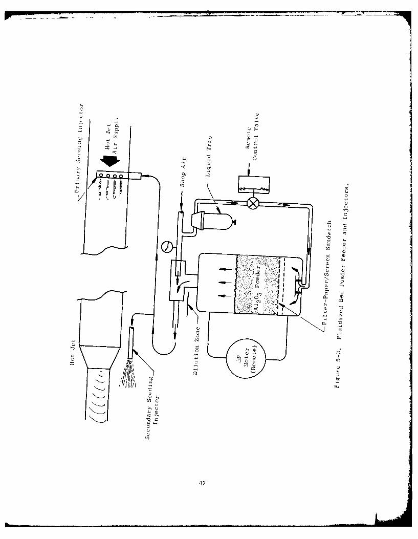
l U2
47~

.+,.: /
.411
,I, )i +°+ C-
NN

0-----
TV Camera
Microphone Network
Laser 0_
Power 'Controls Nozzle Under Test
... . . "-v Mike Attn :
KMarkbIoI andL LV Signal PDP 11145 Select
Processor Minicomputer: S*Multiple Input A to D [Closed 1
Pus egt*Floating Point Processor ]Circuit
Anlzr* Storage: Core Disc Magtape Televistor
and * Keyboard ControlMoir
* Display and Hard Copy Control
Mair k I I and
LV Signal LonitorProcessor
Plot HistogramsPle r He t Plo't Cross-Correlation-
AnalyzeCoefficient:
Plotter * In-Jet/Far Field Mike
* In-Jet/In-Jet
Main X Display Print Tabulation:Actuator YControls Z * Local Mean Velocity
"" - i* local Turbulence VelocityLV-LIV Xl Display
Actuator Yl * Local Correlation CoefficientControls 71
Figure 5-5. Data Acquisition and Reduction.
49

Individual controls are used for each LV. Each LV has its own original
processor assigned. Each processor has its own pulse height analyzer and
plotter.
The General Electric LV processor outputs are also directly linked to a
PDP 11/45 minicomputer system which is used for the following data reduction
and cataloging tasks:
" Log nozzle conditions and plume sensor locations.
* Count and log number of LV data samples per location.
" Plot histogram of velocity samples.
* Plot cross-correlation coefficients (in-jet in-jet and in-jet far-field microphone).
* Calculate and log correlation coefficients, mean and root-mean-square values, confidence intervals, histogram data.
The minicomputer has a multiple input analog to digital converter,
floating point processor, core, disc and bulk magnetic tape storage, keyboard
control, storage scope display and hard copy unit. The data reductions neces-
sary to control the experiment and confirm that adequate data has been
acquired (conf idence interval ) arc performed with in seconds of each data col-
lection interval. This allows the engineer to make a decision for or against
additional IV samples before actuating the L system to the next plume loca-
t ion.
All of the above data is provided on-line during test, and is all filed
in disk storage. The stored data is used later for data reduction for length
and srale of turbulence e, tion velocitv, spectrum of turbu1ence and
derivatives of cross-correlation functions. The data reduction programs used
for on-line data analysis and reduction of the jet's turbulence properties
are discussed in Section 7.0 and 8.0.
~~0

6.0 THEORETICAL AERO-ACOUSTIC FRAME WORK FOR REAL TIME MEASUREMENTS
The problem of performing meaningful turbulent flow measurements for the
purpose of better understanding Jet noise continues to be a difficult one for
technology and physics in general. Until recently, the prospect of performing
real time velocity measurements in realistic jet flows was, practically speak-
ing, impossible. With the advent of today's laser velocimeter, the prospect
has changed and moved in a direction of high feasibility. It is only now
that the acoustic design engineer has at his disposal the type of advanced
instrumentation necessary for performing the type of detailed measurements
needed to better understand and postulate more accurate aero-acoustic models.
Jet noise generation and reduction is directly linked to the aerodynamic
nature of turbulent jets in the form of what is referred to as the "aerodynamic
source team"'. The definition of this term can be analytically described in
terms of direct correlations between the turbulent velocity and the acoustic
far-field pressure, or in terms of turbulent structure properties such as
turbulent length scale, urbulent convection speed, and turbulence spectra of
the moving eddies. The latter turbulence properties can be measured by so-
called turbulent velocity two-point cross correlation measurements. Some of
the governing equations which are used for describing the aerodynamic nature
of jet noise are discussed below.
6.1 GOVERNING EQUATIONS
The generation of aerodynamic noise by free turbulence received its first(27 ,28)
quantitative formulation by Lighthill. The principle quantitative step
by Lighthill was his rearrangement of the continuity and momentum equations
to yield a wave equation.
For the continuity equation we have:
D_ + a(Pui) 0 (6-1)
51

From the conservation of momentum
+ui +3(puiu*) =_- P + - (6-2)
t x 3xi + xJ
Where 'ij is the viscous stress tensor.
From the above equations the following wave equation can be formed:
32p a 2 V2 = -a- (6-3)
Dt2 0 Q - xi
where
Ti= (guiu. - ij) + (p - a O)
Lighthills stress tensor
ao = Ambient speed of sound
p = Fluid Density
Far from the flow region of the jet itself, the right-hand-side of Equation
6-3 must vanish identically leaving the well-known homogeneous wave equation,
which, under homogeneous isentropic conditions, governs linear acoustics in
a uniform medium at rest - the implied "acoustic analogy."
The formal transformation of the differential equation presented above
into an integral equation may be performed using the Kirchhoff integral. For
the pressure perturbation field, one may write:
P'("X,t) = xij jJ U 3 (6-4)4 a21-1 3 t2
V0 t-TO
where the coordinate system is defined in the sketch on the following page:
52
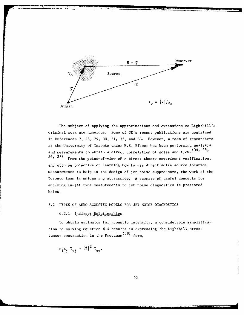
Observer
V0 :! . Sour ce
Origin To 1 x
The subject of applying the approximations and extensions to Lighthill's
original work are numerous. Some of GE's recent publications are contained
in References 7, 23, 29, 30, 31, 32, and 33. However, a team of researchers
at the University of Toronto under H.S. Ribner has been performing analysis
and measurements to obtain a direct correlation of noise and flow.(34' 35,
36, 37) From the point-of-view of a direct theory experiment verification,
and with an objective of learning how to use direct noise source location
measurements to help in the design of jet noise suppressors, the work of the
Toronto team is unique and attractive. A summary of useful concepts for
applying in-jet type measurements to jet noise diagnostics is presented
below.
6.2 TYPES OF AERO-ACOUSTIC MODELS FOR JET NOISE DIAGNOSTICS
6.2.1 Indirect Relationships
To obtain estimates for acoustic intensity, a considerable simplifica-
tion to solving Equation 6-4 results in expressing the Lighthill stress
tensor contraction in the Proudman (38 ) form,
xx T, =IITij ij xx
53

W.T. Chu (37) has shown that the spectrum of noise per unit volume of
turbulence may be estimated using the Proudman approximation:
3 4e_(,24,
I(xf) Tx2 L w4 /e 4 2)Xx x tf(65AV° 16-5/2 a4 i 2 Wf (6-5)
where
Lx, Wf = Typical length scale and frequency of turbulence
Wt = Radian frequency in the turbulence
F oW2 L2 1/2- = -Mc Cos0)2+ ( fx
M = Convection Mach Number of the Turbulent eddyc (V/ao)
T = (o U 2
xx X
Ux = The instantaneous velocity component in the x-direction
U + U (t)x x
Thus, from Equation 6-5, note that, if the point properties of the turbulence(L U x fedaosi ai
(Lx, U, U Wt ) can be measured, an estimate of the far-field acoustic radi-
ation per unit volume of jet can be made. Sections 7 and 8 below describe
the algorithms necessary to obtain these real-time measurements using the
laser velocirneter. Suffice to say here that the mean velocity and turbulent
velocity can be determined by a single point measurement. However, to deter-
mine the convection speed, length scale of turbulence, and the turbulence
spectra of the convecting eddy requires the use of two-point space-time cross
correlation measurement technology.
541

6.2.2 Direct Relationships
In formulating more direct relationships, or correlation between the jet
flow and noise, a number of investigators have formulated unique techniques
which can be used for various applications (see References 35, 36, 37, 39,
40, and 41). Some of the reported work was formulated for correlations of
two pressure signals (References 39, 40, and 41) and others are formulated as
a direct cross-correlation between the source velocity field and the acoustic
(36)radiation field. In particular, the work of Lee and Ribner , and Seiner
and Reethof (4 2 ) are notable. Basically, however, all the techniques advanced
were limited in their demonstration to subsonic ambient jets due to instru-
mentation limitations. The laser velocimeter does not have the limitations
of these older measurement techniques and thus the LV was adapted and de-
veloped for the direct causality type measurements.
To obtain a working relationship relating the turbulent jet velocity
field to the far-field acoustic pressure field, use of Proudman's form of
(35)Lighthill's integral for aerodynamic noise is used again . An illustrative
equation is an expression of acoustic intensity at i due to a unit volume of
turbulence at y.
l(xy) 1 [__ Iu2 (6-6)
0V° 41Ta 3 r LaT (xyT 6-
where
Ru = u2 (") p' (x; 1, T)x P x
TO = Retarded Time (x/ao)
U= - u' (T)
Hence, once the value of R 2 , and the retarded time To are known, in prin-ux p
ciple the acoustic intensity of the noise can be determined. Although the
concept is simple in principle, carrying out the proper measurement using a
55
L iA-M
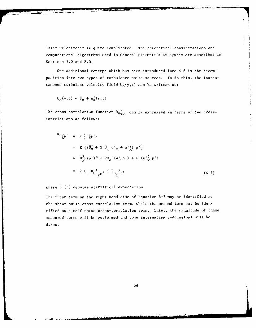
laser velocimeter is quite complicated. The theoretical considerations and
computational algorithms used in General Electric's LV system are described in
Sections 7.0 and 8.0.
One additional concept which has been introduced into 6-6 is the decom-
position into two types of turbulence noise sources. To do this, the instan-
taneous turbulent velocity field Ux(y,t) can be written as:
Ux(yt) = U + u (y,t)
The cross-correlation function Ru , can be expressed in terms of two cross-
correlations as follows:
,2 E x
- E (UX + 2 Ux u'x + u) p l
= U2E(p')o + 2UxE(u'xp') + E (u'2 p')
S2 Ux RuXP' R,2 (6-7)
where E {-} denotes statistical expectation.
The first term on the right-hand side of Equation 6-7 may be identified as
the shear noise cross-correlation term, while the second term may be iden-
tified as a self noise cross-correlation term. Later, the magnitude of these
measured terms will be performed and some interesting conclusions will be
drawn.
56

- ---------
7.0 THEORETICAL CONSIDERATIONS FOR REAL TIME MEASUREMENTSUSING THE LASER VELOCIMETER.
The previous sections have established the importance of mean and turbu-
lence velocity measurements, velocity histograms, and time series statistics
such as velocity spectrum, and cross correlation functions to the aero-acoustic
engineer. This section develops the theory necessary for making these measure-
ments with the laser velocimeter. The reason that special measurement tech-
niques must be developed for the laser velocimeter is that the LV makes dis-
crete measurements randomly in time (measurements are made only when particles
arrive at the probe volume). The traditional theories of measurement apply
only for continuous signals or for signals sampled in equal spaced time
intervals. New theories of measurement are necessary to treat the random tim
sampling that occurs in laser velocimeter measurements.
Two types of measurements (histograms and correlation functions) can be
made from which mean velocity, turbulence velocity, and velocity spectrum
measurements can be obtained.
7.1 HISTOGRAM MEASUREMENTS FROM LASER VELOCIMETER DATA
A histogram is an estimate of the first order probability density function
of the amplitude of a signal. To obtain a histogram, the range of the input
signal, x(t), is divided into classes bounded by values x i. A counter, k., is
incremented for each input if xi <x(t) <xi+ I . This is done for N independent
samples of x(t), such that
kiP. (7-1)
i N
where P. is an estimate of the probability that a sample of x(t) is between x.
and x If the true amplitude probability density function, f(x), doesn't
vary "very much" in this interval, then
57

f= K is an estimate of: (7-2)x N(xi+ - xi)
i+1 i
F(x+) - F(xi)-f(xi)
(xi+ I -x i )
If the successive values of x(t) are independent (that is, if sufficient time
delay has occurred between samples), the probability distribution which
describes the random variable, ki, is the binomial distribution. If pi is
the true probability that x. < x(t) -xi+ 1 , then
K. N-K.P(K. = k.) = ( N) P. (I - P.) 1 (7-3)
1 1 K. i 11
when N independent samples are used to construct the histogram. From this it
may be shown that
E(K i) = PiN; where E {.) denotes statistical expectation (7-4)
so that E(Pi) p. (7-5)
and hence the estimate of the probability that x(t) falls in class (x.,
1
x i+ ) is unbiased. For large values of N (in the present case N will always
be large enough) P(K.) is very nearly normal and may be used to put a confi-
dence interval on k.. Recalling from the theory of Binomial Distributions1
that
VAR(K.) = P.(I-P.)N (7-6)
it can be said with 8% confidence that the "true" value of K. is contained in1
k. Z, Ti(I-Pi)N (7-7)
2
58

If pi is approximated by p, one may then say that the "true" value of K. is1
contained in
Ki ±Z Ki (1- k) (7-8)
2
where Z is related to 8 as shown in Table 7-1.
2
Table 7-1. Relationship of Z to 8.
8 in percent Z a/2
90 1.645
95 1.960
98 2.326
99 2.576
The equations stated in this section may be used to estimate the number of
points required for a histogram with a given level of precision.
If the fractional error for the i-th class is defined at some level of
confidence 8% as
Pi - Pie.(8) (7-9)
then using the result of Equations (4) and (8) it may be shown that
el(8) < Z_ 4 i) (7-10)
2
where pi is the probability that a given x(t) falls in the interval (xi ,
x i+l). At 95% confidence one can then generate Table 7-2 which shows the
total number of data points, N, required to obtain a given error as a function
of class interval.
59

Table 7-2. Data Points Required.
Percent Error
20% 10% 5% 2.5%
.2cwidth I 1156 4624 18500 74000Class IntervalJ P + a 1967 7868 31470 125883Centered p + 2a 9112 36443 145770 583084at w p + 3a 111,222 444,889 1779556 7182240
Number of Points N
7.1.1 Guide for Obtaining Histograms
When obtaining histograms one should observe the following points:
a. For the histograms to be useful in estimating higher order moments(mean, var, etc.) the classes must be sufficiently fine. Bendat(43)
suggests that the class width Ax < .2G everywhere except at thetails for the means and variances.
b. To have sufficient data for testing, mean computation, etc. the
experiment should be planned so that ki > 5 for each class. Tofacilitate this, each tail may be made a class, as shown; allother intervals have widths of 0.2n.
First Class Last Class
X1 x 2 X3 x 4 x5 x 6 x 7 X8
c. If a "histogram analyzer" is used with a countertype laser veloci-meter processor with a digital output, a bias error may occur dueto the mis-match of quantizing steps between the analyzer and thedigital device. For an example of this error, see Reference 44.
d. Use enough data to obtain sufficient accuracy in the histogram,depending on the purpose for which this data will be used where Zc/2
is related to (1 as shown in Table 7-1. Tables 7-2, 7-3 and 7-4should be useful in determining N before the data is collected.
60

7.2 STATISTICS DERIVED FROM THE HISTOGRAM
Several useful statistics may be derived directly from the histogram.
Among these are the mean (average velocity) and the moments about the mean
(central moments). The set of central moments contains the variance and
standard deviation (turbulence level), skewness and "Kurtosis" (peakedness).
7.2.1 Mean
Recall that the mean or expected value of a discrete random variable is
defined as:
N
x= E(X) = E xi P(X. = x.) (7-14)
i=l
This may be estimated using the histogram. Recall that
k.
(7-15)i N
is an estimate of
P(xi < x(t) < xi+I), the probability that x. <x(t) < xi+ I
Thus if the class intervals are small enough, one may estimate the mean as
x = ( i + l + Xi k i
+2 k
all2 N
intervals
x x.x i+l + iwhere is the value at the center of the class interval.
k. is the number of counts in that class.
and N is the total number of points in the histogram.
7.2.2 Moments about the Mean
The Zth moment about the mean is defined as
E{(X - x)iEx
(i1

* T_
After computing x, one may estimate the Zth moment about the mean, mV, as
N 2 X N- (7-16)
all class
intervalsi
These estimators are biased, but for large n (as in all GE LV histograms)
this bias is negligable(45)
7.2.3 Variance
When Z = 2, Equation 7-16 gives the variance. The square root of this
estimates the standard deviation (or turbulence).
7.2.4 Skewness
When k = 3, one obtains the third moment about the mean. This moment is
required to calculate the correlation coefficient betwe,.-; jet velocity squared
and acoustic pressure.
If m3 = 0, there is no skewness (the distribution is symmetric:
If 3 0
If m 3 < 0, the distribution skews to the left:
If m3 20 the distribution skews to the right:
62

The "Skewness" (a z in the literature) is normalized so that it is in-
dependent of scale and is calculated as
a3 3 (7-17)3] 3/2m
2
7.2.5 Kurtosis
When Z = 4, the moment relates to the peakedness of the distribution.
This moment is required to calculate the correlation coefficient between jet
velocity squared and acoustic pressure. The normalized version of this
static is called a4 and is calculated as
a m 44 = (7-18)
m 2
If the distribution is Gaussian,
ax4 =3.0
If the distribution is uniform
Ct 4 = 1.8
Sometimes a4 is called the Kurtosis and other times, the Kurtosis is
defined so that the Gaussian distribution has zero Kurtosis, i.e.:
a 4 = 4 - 3 (7-19)
(3
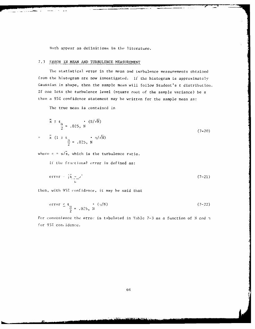
Both appear as definitions in the literature.
7.3 ERROR IN MEAN AND TURBULENCE MEASUREMENT
The statistical error in the mean and turbulence measurements obtained
from the histogram are now investigated. If the histogram is approximately
Gaussian in shape, then the sample mean will follow Student's t distribution.
If one lets the turbulence level (square root of the sample variance) be s
then a 95% confidence statement may be written for the sample mean as:
The true mean is contained in
x ± t • (S/sK)- = .025, N2 (7-20)
x (I ± t • VIN)
= .025, N
where q = s/x, which is the turbulence ratio.
If the fractional error is defined as:
error = x - (7-21)
then, with 957 confidence, it may be said that
error < t (11/N) (7-22)2 .025, N
For convenience the error is tabulated in Table 7-3 as a function of N and Ti
for 95Z coniidence.
64

Table 7-3. Error Percent in Mean Measure-ment with 95% Confidence as aFunction of N and n
.2 .1 .05 .025
10 14.1 7 3.5 1.76
20 9.3 4.7 2.3 1.2
30 7.4 3.7 1.9 .93
40 6.3 3.2 1.6 .8
60 5.0 2.6 1.3 .65
120 3.6 1.8 .9 .45
In a similar manner, one may find the fractional error in the estimate
of the turbulence, S. If the histogram is roughly Gaussian,
S 2 (N- 1) 22 - N-1 (7-23)a
where 2 is a chi-square random variable with N-1 degrees of freedom. Thus,
a confidence interval on the true turbulence, S, is then
S N-I > a > S pf 1 (7-24)
.025, N S Xa = .975, N
with 95% confidenc2. The worst fractional error (since the tails of the Chi-
square distribution are unsymmetric) is then
error = IS - al < X .025, N-I -1. (7-25)a (N-l)
The percent error at 95% confidence for various values of N is presented
in Table 7-4.
65
It

Table 7-4. Fractional Error in Percentfor Turbulence Estimate as;n Function of N.
N Error Percent
20 31.5
40 21.8
60 17.8
120 12.6
240 9.12
480 6.45
960 4.56
5000 2.0
25,000 .89
Examination of Tables 7-3 and 7-4 shows that considerably more data must
be processed for a turbulence estimate than is needed for a mean velocity
estimate of equivalent accuracy. When measuring the skewness or Kurtosis,
similar increases in data for equivalent accuracy will be required over the
turbulence estimate. Also, the biac' due to class interval width will in-
crease and the Bendat rule of .27 wil' :robably have to be tightened. It is
difficult to get estimates of skewness and Kurtosis repeatable to less than
several percent.
7.4 CORRELATION FUNCTION MEASUREMENT WITH THE LASER VELOCIMLTER
The measurement of correlation functions with the velocimeter is impor-
tant because it extends the usefulness of the tool allowi:,g it to perform
measurements of turbulence spectra (obtained by Fourier Transformation of the
velocity auto correlation function), turbulence eddy convective Mach number,
turbulence length scale, the spectra of turbulence in the moving frame (this
information can be obtained from cross correlation between the velocity at
two points in the jet), and causality (the Lee-Ribner approach requires the
cross correlation between the jet velocity squared and the far field pressure).
These measurements require that a special analysis procedure be developed for
66

the laser velocimeter that accounts for the random sampling. This section
presents a method developed at General Electric that has been successfully
used to determine the important aerodynamic and acoustic parameters enumerated
above.
The procedure is developed in detail for the autocorrelation of the jet
velocity, x(t). An explanation is then presented to show how the estimator
can be modified for determining the cross correlation of the velocities at
two points in the jet and for determining the correlation function between
the jet velocity and a continuous signal such as that obtained at the output
of a microphone.
The approach considers the assumptions of wide sense stationarity and
ergodicity made in all methods of spectrum analysis. Wide sense stationarity
prescribes that the values of the autocorrelation function (ACF) are functions
of the time between the signal samples and not the times the samples are
taken. Hence, the ACF of the signal, x(t), is written as
R xx(T) = E {x(+)x(t+T)} (7-26)
where E{-} denotes expectation. If the signal x(t) is ergodic, one can
interpret the expectation as an average over time. Therefore an acceptable
estimate of R xx(T) for some particular value of T might be
M
R(T) + I L X(t k ) X(tk + T) (7-27)XX Mk kk=1
where the tk are M random times at which samples are taken.
Note that Equation 7-27 could be obtained by considering the relationship
between the ACF's of the signal before and after sampling .6,47) If the
sampling process is modeled by a signal, x(t), consisting of impulses occurring
at the sampling times, then the sampled version of x(t), which is called y(t)
can be written
y(t) = x(t) X(t) (7-28)
67
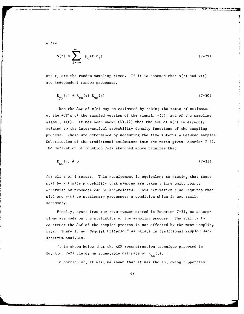
where
S (t) =2 (t-ti (7-29)
and t. are the random sampling times. If it is assumed that s(t) and x(t)1
are independent random processes,
R (T) + R (T) R (1) (7-30)yy Rxx ( ss()
Then the ACF of x(t) may be estimated by taking the ratio of estimates
of the ACF's of the sampled version of the signal, y(t), and of the sampling
signal, s(t). It has been shown (43,44) that the ACF of s(t) is directly
related to the inter-arrival probability density functions of the sampling
process. These are determined by measuring the time intervals between samples.
Substitution of the traditional estimators into the ratio gives Equation 7-27.
The derivation of Equation 7-27 sketched above requires that
R (r)#O0 (7-31)ss
for all T of interest. This requirement is equivalent to stating that there
must be a finite probability that samples are taken T time units apart;
otherwise no products can be accumulated. This derivation also requires that
s(t) and y(t) be stationary processes; a condition which is not really
necessary.
Finally, apart from the requirement stated in Equation 7-31, no assump-
tions are made on the statistics of the sampling process. The ability to
construct the ACF of the sampled process is not affected by the mean sampling
rate. There is no "Nyquist Criterion" as exists in traditional sampled data
spectrum analysis.
rt is shown below that the ACF reconstruction technique proposed in
Equation 7-27 yields an acceptable estimate of R ().xx
In particular, it will be shown that it has the following properties:
68
. . .

1. It is unbiased.
2. It has finite variance.
3. The variance goes to zero as the number of samples in the estimategoes to infinity, i.e., the estimate converges in the mean.
Thus the estimate satisfies the conditions necessary to be called
consistent.
It is easy to show that R xx T) will be an unbiased estimate of R xx(T)
since
M(T)= E{X(t )X(t +r)} = R (T) (7-32)
E{R __a k k xx
k=1
One may now derive the variance of the ACF estimate given in Equation
7-27 by first writing:
M M
E f2 (T} 11 E{X(t.)X(tj)X(ti+1)X(tj+T)}
i=l j=l
MI M2 E{X 2 (ti)X 2 (tj)}
i=l1
M M+ -L2 E{X(ti)X(tj)M t i+T)X(t +T)}1( -3
j (7-33)
i~j
where the expectation is over x(t); and t. and t. given samples at t.+T and1 j 1
t .+T.J
If it is assumed that x(t) is jointly normal and zero mean, the result for
the expected product of four normal variables can be used to simplify the
summations. With
69

E{X(t)X(t+t)} =RXX
one has:
E{R (R) -2 (0)+2R 2 M + EMIi2~E { k 2 ( 1 )} = xx xx + E Ii Rj 2
xx M (t)- M2 xi--I j=l
(7-34)
+Rxx (t i-t j+r)Rxx (t i-t -r)]
where the expectation is over (ti-t.) given samples at t.+T and t.+T. The
first term in the summation gives us (1-i/M)R xx2(T). Combining this withthe term outside the summation, and subtracting the square of the expected
value of the estimate yields
R2 (0)+2R2
(T)VAR{R ({)} = X X
xx M (7-35)
M i-
+Et 2 E ExxR (ti-tj)+Rx (t -t j+T)Rxx(ti-tj -T
)
i-tj i=2 j=l
This is a general result for the variance of the estimator. Written in
this form, the first term represents its variance if all of the product pairs
in the estimate are independent. The second term represents the increase in
the variance due to redundant information in the product pairs. Therefore,
if the samples are taken far enough apart so that
R (tj-t = 0 all t t (7-36)
the variance of the estimate is
R2 (0)+R 2 (t)
VAR(k () - M XX (7-37)
This result may still he a good approximation to the true variance if
the mean arrival rate of product pairs (generally much less than the nean
70
Nami

sampling rate) is less than the reciprocal of the length of the correlation
function of x(t).
While Equation 7-35 gives a generic result for the variance of the AFC
estimate, it is of little use in performing "engineering" calculations of the
error in laser velocimeter correlation functions. However, experiments at
General Electric have shown that the particle arrivals closely follow a
Poisson probability distribution. Assuming a Poisson distribution allows
considerable simplification of Equation 7-35 and provides some simple rules
for estimating errors in correlation measurements.
Obtaining the result for the Poisson sampling case is simplified by the
fact that the subset of samples at times ti, with a sample in [t'+T-A/2,ti
+T+A/21, is also a Poisson process. The mean arrival rate for product pairs
can be shown to be
X' = X2A (7-38)
where A is the "time grid width" representing the amount of deviation allowed
in selection of products lag T apart, and A is the mean rate of the original
Poisson process. The reason for the time grid width, A, is that the prob-
ability of taking two samples exactly T apart is zero. Thus in any practical
realization of Equation 7-27 one must lump together those samples which occurA A
T- T<T+- apart. Averaging product pairs at close to the same lag value
results in the addition of a "time" grid jitter error to the estimate.
Fortunately it may be shown that this error may be made negligibly small if A
(44)is small enough
To simplify the derivation of the bound, one can assume with no loss of
generality that the ti's in Equation 7-35 are ordered so that
t.>t. when i>j
One may then write Equation 7-35 in terms of the inter-arrival density functions
of the Poisson process. These are
71
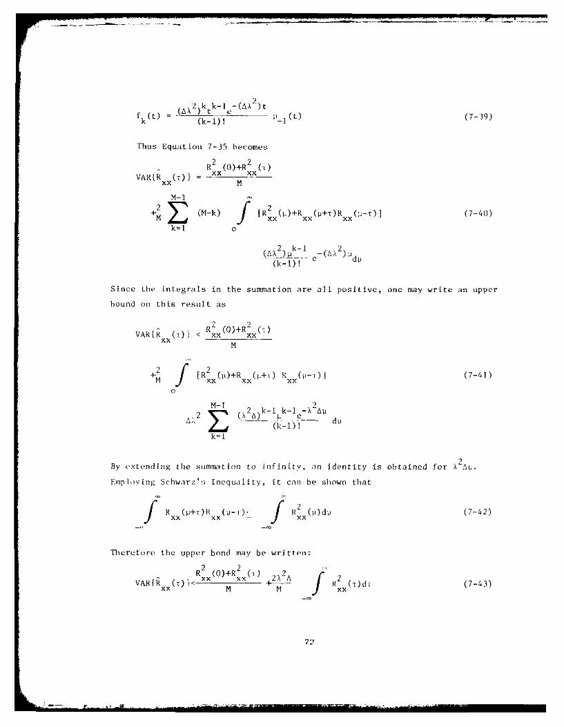
2 k k-I -(AX 2)tf()=(AX )t (739k (k-i)! p()(-9
Thus Equation 7-35 becomes
R 2(0)4-R 2(T)VARtR xx(T)1 = N-Mx
M-1
2 (M-k) [R 2 (ji)+R (p~+T)R (',I-T)] (7-40)M J xx xx xx
k=l 0
2 ) Pk-i e A 2) W(k-I) !e
Since the integrals in the summation are all positive, one may write an upper
bound on this result as
R(0)+R (T)VAR{k (r)} I xx xxxx
2 f [R 2x ()+Rx('+T) R (1I-T)J (7-41)
0
2 - ( 2 k-i k-i -x2 AP2 E (AA) ii e i2~ (k-i)!k=1
By extending the summation to infinity, an identity is obtained for 2 Au.
F'phwing Schwarz's Inequality, it can be shown that
R G+)R (-0-- R 2 (Pd (7-42)
Therefore the upper bond may be written:
R 2(0)+R 2 t 4 2VRkxx xx 2A A R 2 udi(-3VA{R (t} M M Rxxd 7-3
72
This is the upper bound for the variance of the ACF estimate in Equation 7-27
when the sampling is the Poisson process.
Consider the significance of the two terms in Equation 7-43. Note that2the first term is independent of A and that the second term depends on A
Thus for the low mean sampling rates, the first term dominates and the variance
is the same as for the case where all product pairs in the sum are independent.
Now if A becomes very large so that the second term dominates,
2VAR{R2x(T)} ^ 2X2A A R 2 (p)dp (7-44)
xx II
If TL is defined as the length of time over which the observations are taken,
then TL = M/A 2A and
VAR{ ()} k2 R 2 (T)dT (7-45)xx TL xx
If the mean arrival rate is very large, successive samples are highly correlated
and the variance is reduced as the observation time increases. In either
case the variance goes to zero as the amount of data processed increases so
that the estimate is always consistant.
Usually, the laser velocimeter's mean particle arrival rate is less than
10,000 particles/second. For most jet flows, it can be shown that the first
term of the variance equation dominates the second. Thus for engineering
purposes, the variance of the AFC estimate can be approximated by
R 2(0)+R X(T)xx xVAR{R () (7-46)xx M
This can be used to construct confidence limits on the estimate if R xx() is
assumed to be roughly Gaussian. With this assumption, a 98% confidence
statement can be written as
73

R xx(0)+R2 (0R (T) -2.33\XXxx
< R (T < (7-47)-xx -
R X(O)+R (TRxx ) +2.33 M
The estimation procedure given in Equation 7-46 can be extended so that
the cross correlation between the outputs of two laser velocimeters can be
determined. This is done by simply accumulating cross product pairs:
R () = ; X(tk)Y(tk+r)(7-48)
k=l
The procedure can also be used to cross correlate the output of a laser
velocimeter with a continuous signal. In this case, let v (tk+T) represent
the continuous signal that is physically sampled (using a sample and hold
circuit and an A/D converter) at time tk+r. For a particular value of T, a
delay circuit can be used to cause the occurrence of this sample when a
particle arrives at the probe volume at tk'
The procedures described above have been used successfully at General
Electric to determine the auto correlation function at a single point in a
Jet, the cross correlation function between two points in a jet and the
cross-correlation between the je velocity and the _jet velocity squared and a
far field microphone signal.
7.5 MEASUREMENT OF EDDY (ONVECTION VELOCITY
Cross-correlation data obtained between the outputs of two laser veloci-
meters can be used to determine the velocity of turbulent eddies in a jet.
To do this, a set of several correlation functions are obtained with the
laser veLocimeter probe volumes at different spacings, .. For the i t
correlation function, the lag value corresponding to the peak in the correla-
tion function, r. is determined. Thus
7,1

i. is the value where
R (T) is maximum (7-49)
Physically, Ti is interpreted as the time required for the eddy to travel
from the first laser velocimeter to the second. Since the eddy has traveled
the probe volume separation distance in this time interval, an estimate of
the eddy convection velocity is
V =- (7-50)
i T.1
An improved estimate of eddy velocity is obtained by considering a series of
such measurements. If the points (Ti, i) were plotted for a set of N such
measurements on a piece of graph paper, the eddy convection velocity, V c,
would be slope of the best line that could be drawn through the points. Thus
when determining V from a set of correlation functions, the standard linearc
regression formulas can be employed:
lET. T (7-51)
i=
and
(T C )F.i
V = (7-52)c NT i- T) 2
i= 1
The convective mach number can be estimated by dividing V by the appropriatec
jet velocity.
75

7.6 D)ETERMIINATION OF TURBULENCE LENGTH SCALE
Turbulence length scale can also be determined from a set of velocity
cross correlation measurements obtained at different separation distances.
The procedure used is given in Ilinze (48). e i n i ng the ensemble of correla,--
tion functions as
xy j 1
where ris the time lag and FIis the separation distance, one can form the
longitudinal correlation coefficient
f( ' y (7-54)
xx yy
by evaluating each correlation function obtained at T=O. The integral length
scale isi then given from
L f(4)dr (7-55)
0
This integral is approximated Ly fitting a curve of the form
f a exp(7-56)
to the data points f ( ) iig the Conjuigate Gradient (4)procedure. The
Function, f ( , is thun tutitrical Iv integrated using the s impson 's rule
procedure. Gaussian Qiiad rat tire in tegra tion conuld aliso he emp loyed to d irec t 1
obta in 1, from thet .x
7. 7 DFIE R I NATION OF LAGRANGI AN- T1 MEF CORRELATION
A ;cries of two-po n t ye otoo cvorrela t ions at different s-eparation
d(1 t n ce s , lCan aliso he tved to dottermin tiLhe time correl ation function of
an e('(11 in the mnovinrg rote renc f ramc'. S ince the separa tion (list ance *
7 6

and the lag in the moving frame ti are related by the convective eddy velocity,
it is true that the peak values of the cross-correlation functions represent
respective values of the moving frame eddy correlation function. With RL(t)
defined as this LaGrangian correlation function,
R,(til - MAX{Rxy (T, i)}
where ti = the value of T where the maximum occurs.
The spectrum of the eddy in the moving frame can be determined by
taking the Fourier transform of the above.
77

ADAD 2OB GENERAL. ELECTR~IC CO CINCINNATI ON AIRCRAFT ENGINE BROUP F/6 20/1AflA HIGH VELOCITY JiET NOISE SOURCE LOCATION AND REDUCTION. TASK 3. --ETC(U)
DEC 76 P Rt KNOTT. P F SCOTT, P W MOSSEY DOT-OS-30034I CLSSIFIED R78AE627-VOL-4 FAARD-7679-3-4
E-EEIIIIIEE-inIIIIIIIui-- IIIu---

8.0 DESCRIPTION OF GENERAL ELECTRIC'S COMPUTATIONAL ALGORITHMS
Two computer programs have been designed to perform the collection and
correlation of the test data. The program INJET/INJET handles data from two
laser velocimeters (LVi and LV2); and as the name implies, it is used to corre-
late velocity data from two points in the jet stream. The second program,
INJET/FARFLD, operates on data from a single velocimeter (LVI) and data from
a far field pressure transducer (P2).
Both programs employ a data collection and summation module written in
assembly language for efficiency iith regard to execution time. The input
data are quantized to 32 levels, and a technique called quantized product
factoring is used to defer the multiplication process until a point in the
data processing when real time computations are not required.
Prior to the start of the data summation portion of both programs, an
estimate is made of the mean and variance of each input. This is done by
reading 128 samples, summing each input and summing the square of each input
in double precision integer form. The mean is used as a reference or DC
level for all subsequent data inputs and calculations. The variance is found
from ZV 2/128 - V2 and is used in determining the cell size to be used for
quantizing. A cell size equal to 3/16v ariance assumes that 32 levels will
encompass 99% of the total input range for a normal distribution.
Although the two programs are similar in structure, the details of the
data collection and summation differ. For clarity, the two programs will
be discussed separately.
8.1 QUANTIZED PRODUCT FACTORING
Quantized product factoring might best be described by the following:
The normal expression for the sum of products is:
mxiYi
i= 1
78

If the variables x and y are quantized to N levels, there are N finite values
that the quantized variables, X and Y, can take on. This means that the
product can now be factored, and further that the quantized values can be
used as an index or pointer into a vector. The quantized factored form of
the sum of products is
n., Y where k =M~ J=l
j=l j=N
Quantized factorization means that sumnations may be used instead of multi-
plications during that portion of the data processing which is being done in
real time.
8.2 INJET/INJET DATA COLLECTION
All velocity data is collected using an interrupt technique. When a
velocity data point is obtained, that is, the LV circuitry has indicated that
the A/D conversion is complete, an interrupt is generated in the computer.
Four words are read from the digital input device in response to each inter-
rupt, T1, V1, T2 and V2 in that order. Ti and T2 are the external clock times
at the start of the A/D conversion, V1 and V2 are the A/D output values.
Since either LV can generate the interrupt, the sign of the velocity word
causing the interrupt is forced to a 1 to indicate valid data.
Input data for each LV is stored on stacks of 1024 words each. This
allows room for 512 time and velocity pairs. A counter keeps track of the
remaining room on each stack, and a pointer locates the next open location on
each stack. When these pointers reach the bottom of the stack, they are reset
to the top of the stack as long as the counter indicates space available.
79
LA

The time value is placed on the data stack directly. The velocity
value put on the stack is a quantized velocity relative to the mean or DC
level, i.e., Ql = (Vl - Vl)/CSl where CSI is the cell size for LVl.
This data input process goes on independent of the correlation process
which will free locations on the data stacks as the data is used, with the
oldest data being processed first.
8.3 VELOCITY CORRELATION AND HISTOGRAM ALGORITHMS
The correlation process is a pairing of each data point on one stack with
all data points on the other stack whose time differnce (AT) satisfies some
predefined criteria. A total of 512 lag values (AT=T2-T1 ) was chosen, result-
ing in a range for AT of -256 < AT < +255.
A rectangular array, 32 columns by 512 rows, is used to sum the results
of the pairing process. The AT value is used as a row pointer, since each
row corresponds to a specific lag value from -256 to +255. Each column cor-
responds to a quantizing level from -16 to +15. When a pair of data points
is found which meets the AT criteria, one quantized velocity (say Ql) is
used as a column pointer, AT as the row pointer, and Q2 is added into the
specified array element. This is using the quantized factorization technique
described previously. Histograms for each velocity are formed by using the
paired Q values as pointers into vectors 32 elements long and incrementing
the corresponding elements. The number of occurrences of each lag value is
generated in a similar manner by using AT as a pointer into a 512 element
vector and incrementing the indicated element.
When data points on one stack do not pair with any points on the other
stack, the locations they occupy become available for input again. This pair-
ing and summing process is continued until some predetermined number of data
points has been processed, usually 20,000 to 30,000 points; then, all data
input and processing is halted. This is done to prevent an overflow from
occurring in the summing array.
Another interrupt is used to detect the overflow of the external clock.
When the clock overflows, data input is temporarily halted until all the data
80

currently on the data stacks have been correlated, then the data input and
processing is resumed again. This is done because the time information be-
comes ambiguous after a clock overflow unless a double precision clock
counter is used.
8.4 DATA COMPRESSION AND INTERMEDIATE DISPLAYS
When the required number of data points has been examined and process-
ing halted, the summing array is compressed to a double precision vector.
This is done by multiplying each column of the array by its corresponding
quantized velocity value and summing across the columns. In this manner, the
more time consuming multiplication process is done at a point where execution
time is not critical. The double precision vector now contains the sum of
the quantized product pairs for each lag vlaue (AT).1
New estimates of the mean, variance and cell size are calculated for
each velocity from the histogram data. The histogram data are then normalized
and displayed on a scope for operator monitoring.
The current cross-correlation contribution is calculated from the double
precision sum of the product pairs and the previous mean and cell sizes.
The total run correlation coefficient is then updated along with the total
mean and variance values. A normalized correlation 7oefficient is then cal-
culated and displayed on the scope. The number of data points in each histo-
gram along with the total number of data points processed in the run is also
displayed on the scope.
A new DC level is calculated using the latest value of the mean, all
buffers are cleared and the data collection and summing process is resumed
again.
This processing of data, in groups of 20,000 to 30,000 points, is re-
peated until a total of approximately 300,000 points have been sampled, and
then the run is terminated. Although the segmented processing is required to
prevent overflows in the summing buffer, it also allows the quality of the
data collection to be monitored at intervals during the run. This means that
bad data can be detected earlier and the run aborted, rather than at the end
of a complete run.
81

8.5 INJET/FARFLD DATA COLLECTION
Pressure data are obtained on an interrupt basis from a separate A/D
converter that is part of the 11/45 computer system. The conversions are
initiated by signals from the external clock that is part of the laser veloc-
imeter circuitry. When the conversions are complete, an A/D interrupt is
generated. The external clock rate is divided by 4 so that the pressure
interrupts will occur at a 20 KHz rate. The 11/45 clock is set up to gen-
erate a clock interrupt when the external clock overflows. A software clock
is used internally in the program and is incremented every time a pressure
interrupt is serviced.
Velocity data are obtained through the same digital input device that is
used for the INJET/INJET program, except that only one velocimeter is used.
A device flag is set rather than generating an interrupt when a new sample of
velocity and time is ready.
The down stream separation between the velocimeter and the microphone is
converted to a delay time in clock count units using the speed of sound in
the test cell and the clock frequency. This value is reduced by 256 counts
so that a time window for correlation is centered at the mircophone.
When each velocity and time pair is read, the velocity is placed on a
delay stack, and the time value, increased by the delay counts, is placed on
a start time stack. A delay stack counter is decremented to show one less
space is available on the delay stack. When the software clock matches the
start time, the corresponding velocity value is removed from the delay stack,
512 counts are added to the start time to form a stop time, and this value is
placed on a stop time stack. The velocity is then paired with the next 512
pressure values as they are read in the pressure interrupt routing.
8.6 VELOCITY-PESSURE CORRELATION AND HISTORGRAM GENERATION
The correlation of each velocity-pressure pair is done entirely in the
pressure interrupt routine. The quantized factoring technique is utilzed to
defer the actual multiplication operation. A quantized velocity, Ql, is
formed as indicated in Section 8.2 and is used as a column pointer into the
summing array.
82

The summation is done entirely within the pressure interrupt routine.
In response to each pressure interrupt, the A/D value is read and a quantized
pressure, Q2, is formed in a manner similar to the velocity quantizing. In
this case, no subtraction of a DC level is made; since, by definition, the DC
pressure level is zero.
Implied in the definition of the time window and, therefore, the start and
stop times is that, at the start time At = -256 clock counts and at the stop
time At = +255 clock counts. Therefore, when a velocity value is "started",
At can be thought of as pointing to the first row in the summing array. The
quantized pressure Q2 can, therefore, be summed into the first element of the
column pointed to by the quantized velocity Ql.
Since each pressure interrupt will occur one clock count later, the next
Q2 value will be summed into the next element of the same column which corre-
sponds to At = -255. This summing process is continued until the clock time
matches the stop time for this velocity value or 512 clock counts later.
The pressure interrupt routine is coded to handle four of these summing and
auto-indexing sequences, which are referred to as accumulators. Therefore,
four different velocity values can be paired with the same pressure value.
Twelve velocities may be waiting on the delay stack.
When a velocity is "started", it is removed from the delay stack and the
delay stack counter is incremented to indicate an available location for a
new velocity. A check is made to see if an accumulator is available. If all
accumulators are in use, the velocity value is discarded. However, if an
accumulator is available, the quantized velocity, Ql, is used to increment
the velocity histogram as described in Section 8.3, the stop time is calcu-
lated and stored on the stop stack, and the processing counter is incremented.
This is the counter that is used to halt processing when 20,000 or 30,000
points have been processed. The accumulator chosen is loaded with the Ql
value and enabled so that during the next 512 pressure interrupts it will be
active.
When the clock value matches a stop time, the corresponding accumulator
is turned off and the last quantized pressure value is used to increment the
pressure histogram.
83
External clock overflows generate an interrupt which causes the software
clock to be reset to zero. To prevent this from happening while any accum-
ulator is running, a velocity value will never be put on a delay stack if the
delay time plus the accumulated time will exceed the remaining time in the
current clock cycle.
8.7 DATA COMPRESSION AND DISPLAY
The compression of the summing array to a double precision vector con-
taining EQl*ZQ2 is accomplished as described in Section 8.4 for the INJET/
INJET program. An additional step is introduced so that the sum of Q12*Q2 is
formed for each lag value.
The remainder of the calculations and display generations is essen-
tially identical to the procedure described for the INJET/INJET program.
84 /
9.0 EXPERIMENTAL ARRANGEMENTS USED FOR LASER VELOCIMETER MEASUREMENTS -
GENERAL ELECTRIC ANECHOIC JET NOISE FACILITY
This section contains a brief sketch of the physical experimental
arrangement of General Electric Laser Velocimeter system as configured for
the Anechoic Jet Noise Test Facility.
The nozzle under test and two LV systems are similar to what is shown in
Figures 9-1 and 9-2. The laser beams are highlighted above the nozzle by
nature of the seeding. In the right of Figure 9-1 the two-velocimeter pack-
age may be seen mounted on its main-three-axis (X-Y-Z) actuator. The LV to
the right is installed on an independently operated sub-three-axis (X'-Y'-Z')
actuator that controls the spacing of the twin LV measurement control col-
umns. Control and data acquisition consoles are shown in the photographs of
Figures 9-3 and 9-4. The minicomputer is in the three low cabinets to the
right in Figure 9-3. The keyboard input and printer is at the far right.
The Mark II signal processor is in the left-hand cabinet, and the Mark III
processor is on the lower shelf of the cart. This photograph was taken
before equipment locations were finalized. The console of Figure 9-4 is
mainly for nozzle operation, with the exception of the right-hand cabinet,
that houses the LV actuator controls.
85

Figure 9-1. Dual Laser Velocimeter in Operation ini the GE AilechoicJet Noise Facility.
SC)II

p' tii' 9.IuaiLiser Velociine ter -Closeup Viewv.
87

Figure 9-3. LV Control and Data Acquisition Consoles,
GE Anechoic Jet Noise Facility.
88

F igure-, 9-4. N 11z1 t Cntrol Console, GE Anecho ic

10.0 RESULTS OF MEASUREMENTS
The General Electric Laser Velocimeter system has undergone a series of
electronic and automated data processing developments over the last several
years. For example, within the last two years, new improvements in signal
processing and data processing techniques have increased data taking capability
by a factor of 90 for two-point, space-time type of measurements. Sections
3.0 through 8.0 describe many of the existing improvements and techniques
necessary for performing advanced real-time measurements. References 30, 31,
50 and 51 provide some of the reference material in which has been demon-
strated unique LV diagnostic capability for heated high velocity exhaust
jets.
The first item discussed in this section is a summary of some highlights
of previously acquired mean velocity and turbulent velocity measurements
performed on heated supersonic jets and of turbulence spectra measurements.
Secondly, results are presented of more recently obtained two-point,
space-time, in-jet measurements; and in-jet to far-field cross-correlation
measurements performed on a conic nozzle and a coannular plug nozzle.
10.1 MODEL SCALE MEAN VELOCITY AND TURBULENT VELOCITY MEASUREMENTS
The laser velocimeter measurements reported herein were made in General
Electric's Jet Noise Acoustic Test Facility. Two nozzles were used in the
tests: a converging-diverging nozzle producing shock-free supersonic flow,
and a conical nozzle used for subsonic tests and shock structure measure-
ments. The exit diameter of both nozzles was 6 inches.
The velocity measurements were obtained as probability density distri-
butions and the data were reduced by using statistical techniques discussed
in Sections 7.0 and 8.0 to compute the mean values and standard deviations (mean
velocity and turbulent velocity), respectively. Typical mean and turbulent
laser velocimeter (LV) measurements for an ambient subsonic jet are compared
with hot film/hot wire measurements in Figures 10-1, a and b. LV measurements
of mean velocity and turbulent velocity were then obtained for the high-
temperature (15000 R), fully-expanded supersonic (M= 1.5) convergent-divergent
90
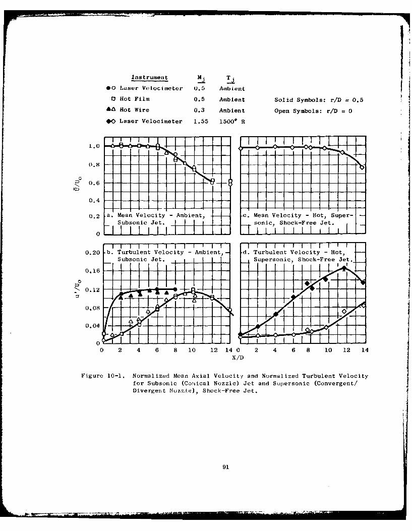
Instrument T
@0 Laser Velocirneter 0.5 Ambient0 Hot Film 0.5 Ambient Solid Symbols: r/D 0.5
A45 Hot Wire 0.3 Ambient Open Symbols: rID =0
QLaser Velocimeter 1.55 1500* R
0.2 a. Mean Velocity -Ambient, -c. Mean Velocity -Hot, Super-Subonic Jet jj j - sonic, Shock-Free Jet.
0 1 11 1 !'7T 1 Aii Ii Ii
0.20 b. Turbulent Velocity-Ambient, -d. Turbulent Velocity-Hot,Subsonic Jet._ Supersonic, Shock-Free Jet.
0.16-- -I-->0.12
0.08
0 2 4 6 8 10 12 14 0 2 4 6 8 10 12 14
Figure 10-1. Normalized Mean Axial Velocity and Normalized Turbulent Velocity
for Subsonic (C3,lical Nozzle) Jet and Supersonic (Convergent!
Divergent Nuzzie), Shock-Free Jet.
91

nozzle. The results of these measurements are presented in Figures 10-1c and
d. In Figures 10-la and c, the existence of the entended potential core for
the supersonic jet is evident. The differences in turbulence distributions
between the subsonic and supersonic jet can be observed by comparing Figures
10-lb and d.
Further experimental measurements were obtained using the converging-
diverging shock-free nozzle flow and the shocked conic nozzle flow. For both
cases, the exit Mach number of the jet was 1.55 and the total temperature was
15000 R. Radial profiles of mean axial velocities were obtained for various
axial locations, X, in the jets of both nozzles. The results, presented in
Figures 10-2a and b, are plotted using the parameter, n, which collapses all
of the data onto one curve and clearly defines the jet boundary and the shear
layer at r = ro. For the conic nozzle case, Figure 10-2b, the under-expansion
in the jet boundary is apparent as the value of the normalized mean velocity
becomes greater than 1.0 in the expansion region near the jet exit plane (X/D
- 2).
Radial profiles of normalized turbulence velocity for the converging-
diverging nozzle are shown in Figure 10-2c as a function of the same variable,
n, (used in the previous figures) and was again used here to collapse all the
profiles onto one curve. The peak turbulence (maximum shear) is clearly
observed to occur at the jet boundary, r = ro .
To complement the above conic nozzle measurements, a series of LV measure-
ments was also made to define the conic nozzle shock structure. Figure 10-3
shows the measured axial mean velocity and turbulent velocity distributions
along the centerline of the jet. The expansion and contraction of the axial
velocity in the shock-flow region are clearly shown. For reference purposes,
predicted velocity is also shown. The amplification of turbulent velocity
due to the shock is also evident.
10.2 TURBULENCE SPECTRA
To construct turbulence spectra from the discontinuous output of the LV
presents a difficulty not encountered with continous type instrumentation.
Conventional point spectra estimate techniques assume that all values of the
92

a. Mean Velocity; C/D Nozzle, b. Mean Velocity; Conical Nozzle,
Shock-Free Data, MI = 1.55, Shocked Data, j= 1.55,
TT = 15000 R. TT 15000 R.IAt 6rvI!1.00 "01.00 2
0.75 1 - il
*10
1*120.50 0.50 -1614-
fl/V 2 VAI 2Uip (-iOx (TI + 0.05) U Zp (-iSOX (in + 0.05)
0.25 0.25- -
0 0
-3.6 -0.6 -0.4 -0.2 0 0.2 0.4
= (r-ro)/(X-D) = (r-ro)/(X-D)
c. Turbulence Velocity; C/D Nozzle,Shock-Free Data, Mj= 1.55,
TT 15000 R.
0.8
9s90.6 <> 2
. 4
E A
012 K614
C
0.2
0
4 -0.3 - .2 -. 0.1 0.2
ri= (r-ro)/(X-D)
Figure 10-2. LV Measured Radial Profiles of Normalized Mean Velocity and
Normalized Turbulent Velocity.
93

a. Mean Velocity.
ii1 OS -- 7C5~2500 __ -______- __
00
1500)
0J 2 3 6 7
Axiq i Os) flhl( X,'R
,T" amb 41.1 - Pre~dicted VuloL 1N
mexit 1.0 0 I.' measurecntu
S30 b. Turbulent Velocity. T T 1500* R
100
0 1 2 3I 4 5 6 7
Axial Dis t avce, X/R
Figure 10-3. LV Measured Mean Velocity and Turbulence Intensity on Center-Line for a High Velocity, High Temperature Jet.
94

input signal are known in the analysis interval. Such knowledge is not
available at the LV output. To overcome this problem, it was necessary to
construct the autocorrelation function of the velocity signal, then obtain
the spectrum as its Fourier transform. Sections 7.0 and 8.0 describe the
theoretical and computational considerations for these types of measurements.
Figure lO-4a shows a comparison of the LV reconstructed spectra with that
using a hot film for a subsonic jet. Figure 10-4b shows the LV measured
turbulent spectra for a sonic (Mj - 1.0) heated (total temperature of 15000 R)
jet. These results were quite encouraging in regard to the real-time
measurement studies. These results gave more confidence to pursue cross-
correlation type real-time studies.
10.3 TWO-POINT, SPACE-TIME, IN-JET, CROSS-CORRELATION MEASUREMENTS
In order to develop the technology of using the laser velocimeter for
performing advanced type turbulence measurements, a combination of signal
processing development, theoretical analysis, computer software data process-
ing techniques and laser velocimeter actuation equipment development was
necessary. Sections 3.0 through 9.0 describe the extent of development
necessary. The measurement of two-point cross correlations with a non-
contact-type measuring device such as a laser velocimeter has never been
performed before. The full accomplishment of such techniques will enable the
measurement and location for an exhaust jet's aerodynamic noise source and
will eventually lead to a new diagnostic device for evaluating and better
designing exhaust nozzle suppression devices.
Discussed below are results of a series of two-point, space-time, in-jet
type measurements in a conic nozzle and a coannular plug nozzle. The
resultant measurements could be used in the aero-acoustic indirect models
described in Section 6.0.
10.3.1 Conic Nozzle Measurements
Although all the computational schemes and algorithms for performing the
two-point, space-time, cross-correlation measurements are covered in detail in
Sections 7.0 and 8.0, it is instructive to briefly review the concepts here.
Sketches shown in Figures lO-Sa and b serve the purpose for the following
95

00
-4 40
$a l
m D u 0
4.U 4.-4u
us * cc 4-)-,4 -4 .- Ca 0
4)
0.~
0- 0)uC
-4 4s
II E,
0 ccF-
0 W 4)i $.
0. (D CS
144.>
Cu '-4
C)4cq to 0
- - op
as 96

2
x,
R =u(fl+ /2,T) u(ri-C/2)
u 01-)
/ f
dw Nl U. -r/D
(1) Lxt (n) R fX-[ rl ,O) dr Turbulent Length Scale
(2) Curve Of F VS. T at -I , lT)= 0: Defines Convection'1 Velocity
(3) J R~ i IW-1
b. Turbulent Properties Defined by In-Jet Two-PartSpace-Correlation
Figure 10-5. Sketches Illustrating the Coordinate System and TurbulentProperties Defined by Two-Point Space-Time CrossCorrelation Masurements.
97

discussion of results. Shown in Figure 10-51) are the concepts necessary to
compute the turbulent length scale, Lx , the convection velocity, Vc , and the
spectra of the moving eddy turbulence. Measurements of the turbulent structure
properties were performed in General Electric Anechoic Jet Noise Test Facility
described in Section 9.0. Figures 9-1 and 9-2 are photographs of the two-
laser velocimeter system built for the following measurements.
For the conic nozzle measurements, two nozzle conditions were tested:
Subsonic (M. = 0.5) ambient, and sonic (Mj = 1.0) heated (TT = 16000 R).
Figure 10-6 shows a sample of six two-point, space-time, cross correlations for
the subsonic ambient conic nozzle. The axial spacings for this test were
r/D = 0, 0.25, 0.45, 0.6, 0.85 and 1.0; where F is the axial separation
distance between the two LV control volumes, and D is the diameter of the
conic nozzle (D = 4.64 inches). The ordinate on each scale is the normalized
cross-correlation function, Rxt, while the abscissa is the normalized time
scale, T Vj/D (where T is the time, Vj the ideal exhaust velocity). From
such a series of cross-correlation measurements, the convective speed and
length scale can be determined as illustrated in Figure 10-5b. Table 10-1
summarizes the results of the conic nozzle measurements.
To illustrate the computation of the convection velocity, Vc, Figure 10-
7 was constructed from the test results shown on Figure 10-6. These results
show that, at an axial location of 4 diameters at T/D = 0.25, the convection
velocity, Vc, is 0.723 Vj for both the ambient subsonic jet and the sonic
treated jet. Summarized in Figures l0-8a and b is the LV measured axial
variation of the turbulent length scale and the radial variation of convec-
tion velocity for the measurements taken. The test results shown in Figure
10-8a show that the turbulent length scales for the subsonic unheated and the
sonic heated jet are much the same. There is, however, a noticeable radial
variation of length scale, but it is not large. Also, the classically quoted
value, LX/D = 0.12 X/D, is at variance with the above-measured length
scales, as well as some University of Toronto hot wire measurements. Instead
of Lx/D = 0.12 X/D, perhaps a more representative equation would be Lx/D
= 0.03 X/D.
The radial variation of convection velocity for the subsonic unheated
and the sonic heated Jet measurements are summarized in Figure 10-8b. These
98

Table 10-1. Summary of Turbulent Properties Measured on a
Conical Nozzle.
a. Subsonic Ambient Conical Nozzle Test Results (Mj = 0.5; Total
Temperature = 5190 R)
X/D r/D V, fps U'/V Vc/Vj Lx/D Lx, in.
4 0 531.4 0.043 0.75 0.057 0.26
0.25 516.3 0.11 0.723 0.091 0.42
0.5 152 0.471 0.414 0.172 0.8
8 0 485.3 0.132 0.809 0.211 0.980.25 390.0 0.215 0.580 0.223 1.03
14 0 304.9 0.195 0.487 0.396 1.84
b. Sonic Heated Conical Nozzle Test Results (Mj 1.0; Total
Temperature 16000 R)
X/D r/D V 1'/V Vc/Vj Lx/D Lx, in.
4 0 1739.7 0.048 0.74 0.0428 0.2
0.25 1511.2 0.10 0.797 0.0934 0.43
where: X = Axial location measured from the jet centerliner = Radial location measured from the jet centerline
Vc = Measured turbulent convective speedV = Measured local mean velocityV4 = Ideally expanded jet velocity
Ul = Measured axial turbulent velocity
U'/f = Local turbulence intensity
99
,,,6 .,il llll I I I I IkI I I

° ii
LI'4 0 0
.4 1
oo
LIP-
- 4 II -,--
00
00
0 0
c o°" 0
0
14
0
0 0
0
0
In In-4
0 0
0~ 0m.
0 O0
-4J
-4.4
1000

* M.= 0.5, Ambient, X/D 4.0 r/D = 0.25
0 M~ -1.0, 16000 R, X/D =4.0, r/D =0.25
2.0 _____
1.5
AA 1.0
0.5
ve/1vi-
0.723
0 I_________ ________
0 0.5 1.0 1.5 2.0
Figure 10-7. Illustration of Method for DeterminingConvective Results of the Two-PointSpace-Time Cross Correlations.
101

- Lx/D =0.13 X/D (Davies et al.)
aM. 0.13, AmbientJt r 1.0, Hot Wire (UTIAS Results)
o M~ 0.5, Ambient Jet, r/D =0
GE Laser Velocimeter0 M. 0.*5, Ambient Jet, r/D = 1.0 Measurements
* M. ~0.1, 16000 R Jet, r/D = 0
* M. 1.0, 16000 Jt r/D = 0.2
0.8 I
a. Axial Variation of Turbulence Length Scale for aConical Nozzle as Measured by a Laser Velocimeter.
0.6
0.
-4e
0.2 I- -____ ___
0 2_____0 2 4 6 8 10 12 14
X /D
1.0 ___
0.8
0 Mj =.5, Ambient Jet, X/D =4
0.6 %00 M.= 0.*5, Ambient Jet, X/D= 8
0 M. = 0.5, Ambient Jet, X/D =14
> U .4 M. 1.0, 16000 R Jet, X/D = 4
b. Radial Variation of Convective Speed
for a Conical Nozzle as Measured by
0.2 a Laser Velocimeter.
00 0.2 0.4 0.6
rID
Figure 10-8. LV Turbulent Structure Measurements for a Conical Nozzle.
102

results show that unheated and heated convective speeds are similar in value,
but there does exist an axial and radial variation in value throughout
the exhaust jet.
10.3.2 Coannular P1y 7j ozeTetRsls
A second series of two-point, space-time measurements were performed on a
second nozzle to explore the type of phenomenon and problems that are encoun-
tered with nozzle systems that are different than the simple conic nozzle.
The second nozzle selected was a coannular plug nozzle configuration illus-
trated in Figure 10-9. Also shown on Figure 10-9 are the two nozzle test
conditions for which the cross-correlation measurements were performed. The
coannular plug nozzle tested was a high radius ratio (RO = 0.85), low area
ratio (A' = 0.33) nozzle tested acoustically under Contract NAS3-19777. This
particular nozzle has been found to exhibit favorable jet acoustic reduction
characteristics relative to a conic nozzle at an equivalent specific thrust.
The test conditions chosen were such that, for the first test point, the outer
and inner streams were slightly less than critical; for the second test
point, the inner stream was maintained at the same conditions as for test
point 1, but the outer stream was raised to a super critical pressure ratio.
Table 10-2 summarizes the results of all the two-point, space-time measure-
ments taken for this test series.
For this coannular plug nozzle, in-jet, cross-correlations were generally
taken at three radial locations for each axial station The locations were
chosen so as to take measurements at the nozzle exhaust centerline, at thepeak velocity location and at a radial location where the local mean velocity
Note that there was a year lapse in time between the conic nozzle
measurements (performed in August 1976), and the coannular plug nozzlemeasurements (performed in August 1977). During that interval, improve-ments in the data acquisition and process were made. Data acquisitionand reduction were improved by a factor of 90.
** Note that at each measurement station (x,r), several axial and separationsof the two LVs are required in order to form the manifold of cross-correlations depicted in Figure 10-5b. In general, the separation distancesused were c/Deq = 0.04, 0.22, 0.39, 0.57, 0.74, 0.92, 1.09, 1.27. Thus, foreach location, approximately seven cross-correlation measurements were made.
103

") U)L) V)
( I 11 ) 1) 1~ 0~ 00 a-C C x 'Ca() 0
-4 ) C.) to -- Q-)4
4 - -4 Q) u).c a) m4
)~M 00- -40
1- E .ONlf~~-o -- 4 U) 4- +
ba) b 4 ' -4 Q) ~'- ) Cl ) C U t- C -lU
N o. l rt- - 'U") N Q) 0) Ln '<<l N 4.) z) U) C .:'c4 *,4) 4
Ez Z -4 4 ' N C
o cz 0 z E 0
4-4 L-4 -04. 5 E5 5 E CO 0 - >
C) C) ) U) % ) -z f)uf >' -4 +
N~. C)) 4-) 4-) 4-)- ) )C.
0- -4 w- 4- w U0 C) C
cu ;. C . 4) C4 > CL a.U
0 ulC 4) -zl z) C" U-) C c
r ) ~C 4 V) N)
..- 4 - 1 L -4 C) C. C.
O _4 4) ) - 4 C CS..~4 04 U) C) U) U)
-4 a) 0. C CLUA. Q0 C0 0 0-E- -- 4 - 4 ~
U)l >l 0. ;. U- ' ~ ' - -
O W 5- + U
-4 .,1 w'- 0 )0N +4 - 4 CL
0 o 0 0- I 0 w
z ~~ ~- -411 t-Cv\ H C
0
0 104

Table 10-2. Summary of Turbulent Structure Properties Measured on a
Coannular Plug Nozzle.
a. Test Point 1 (P = 1.8, TO = 16500 R, V? = 1758 fps, pi = 1.8,
Ti = 8500 R, Vi-- 1250 fps, Vmix = 1602 fps)T j
X/Deq r/Deq U, fps U', fps V c , fps Lx, in. Vc/VT ix Lx/DeqJ
1.81 0.460 1760.0 96.84 1587.6 0.0495 0.991 0.0089
2.54 0.172 1225.2 63.71 1227.1 0.0288 0.766 0.00522
0.241 1370.9 116.53 1297.6 0.1765 0.810 0.03199
0.378 1758.9 91.46 1754.2 0.1715 1.095 0.03107
4.71 0 1098.3 121.9 901.9 0.2098 0.563 0.038
0.329 1606.3 168.66 1510.7 0.3512 0.943 0.0636
0.546 1082.3 284.6 858.7 0.5817 0.536 0.1054
8.15 0 1228.0 136.3 1115.0 1.0089 0.696 0.1828
0.409 1117.8 271.6 842.6 1.1728 0.526 0.2125
0.567 879.5 226.03 765.8 1.5775 0.478 0.2822
9.97 0.181 1145.7 221.1 954.8 1.3886 0.596 0.2516
0.444 1025.8 245.2 746.5 1.4421 0.466 0.2613
0.631 816.0 246.4 730.5 1.7545 0.456 0.3179
b. Test Point 2 (P0 = 2.7, TO = 16500 R, V? = 2216 fps, pi = 1.8,
S r T mix r
Ti = 8500 R, V = 1250 fps, Vj = 1981 fps)
X/Deq r/Deq U, fps U', fps Vc , fps Lx, in. Vc/V j1 x Lx/Deq
2.54 0 608.4 119.8 1010.0 0.212 0.510 0.03845
0.529 1419.6 359.0 1010.0 0.128 0.510 0.02313
0.572 981.9 387.0 1021.0 0.283 0.515 0.05135
4.71 0 1038.8 133.9 1295.0 0.294 0.654 0.05334
0.399 2024.1 151.8 2009.0 0.272 1.014 0.049240.546 1704.2 313.6 1088.0 0.687 0.549 0.1245
8.15 0 1255.8 251.2 1338.0 0.4649 0.675 0.08423
0.314 1456.2 262.1 1403.0 0.9774 0.708 0.17710.634 856.11 290.3 1887.0 1.5105 0.445 0.2737
9.97 0 1265.3 270.8 1271.0 1.2423 0.642 0.2251
105

was approximately 70% of the peak velocity. Figure 10-10 illustrates the
typical mean velocity profiles for test point 1. Illustrated in this figure
is the inverted velocity distribution (high velocity on the outside stream
and lower velocity on the inside stream) typical of this type of test nozzle.
Also shown on this figure are the approximate locations for the cross-
correlation measurements.
Choosing the proper normalization or similitude parameters for the
coannular plug nozzle is not as easily done as for the conic nozzle. For the
coannular plug nozzle, there are two flow streams issuing through annular
gaps. For the turbulent length scale, the outer stream annulus height, h°,
was chosen as the length scale characteristic dimension. For the convection
velocity, Vc, normalization, the ideal outer stream velocity V? was used forJ
locations X/Deq < 5, r/Deq # 0; at r/Deq 0 0, the inner stream velocity, Vj,
was the normalizing velocity used at X/Deq < 5; and the specific thrust,
Vmix, was the normalizing velocity used when X/Deq < 5. Figures 10-11 andJ10-12 summarize the in-jet, cross-correlation turbulence structure measurements
taken to date.
Figure 10-11 illustrates the axial variation of the LV measured turbulent
length scale for the coannular plug nozzle at three streamlike locations:
region of peak velocity, 70% of Local U max' and along the centerline of the
nozzle.
The physical picture which emerges from these measurements is the length
scale of the convecting eddies are smallest along the centerline, largest at
the 70% Umax stream line and intermediate in length along the Umax stream
line.
Figures 10-12a and b illustrate the convective speeds for the two coannular
plug nozzle test conditions. The physical picture illustrated by these
results is not clear. In general, it might be postulated that the larger
eddies moving at the 70% Umax stream lines are convecting at the slowest
speed (Vc -0.4 - 0.66 V9H, while the smaller eddies moving along the center-
line and at Umax are moving along at a faster rate relative to the chosen
characteristic velocity (Vc 0.4 , 1.0 VCH), with the higher convection
speeds occurring closer to the nozzle (X/Deq < 5). One conclusion which can
106

000
E-44
0 0 4.4
-4 P4.)
00
:9 04
M 0
0. 14 $
0I IL) :I
,4 14
4.4)-4
0 04
CUd
-4 eq -
44
00
.0 W)
-4 -44
.4
0 -4
0107
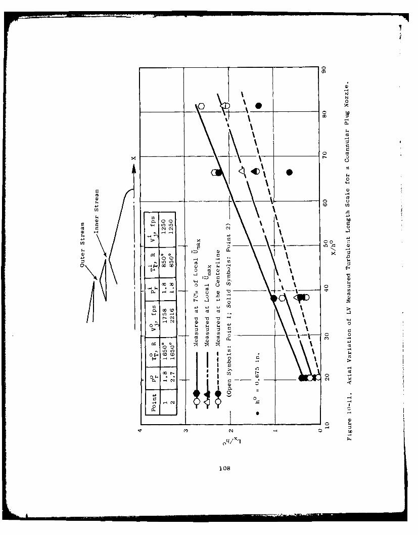
0
ca
04
coNQ)N
4-4 tO 1-4
> CUQ2 00
CD 0 0
4
C co)
U)U
4-4 LO
I,.- t - 4U0 -4-44 *0 r-UCInl ( Cl) -
Il t~ W -4 ;
00 *d Vt4
C U C f 04--4
0 -4 CU
LI) IIL)CU
-4
010

Outer Stream
0.7V~ 07V oraXD < ~ Inner Streamch V or /Uma -1eq-<
Vj ~ ~ ~ ~ a (Deq = 5.519 in.) ..................................................
V3 x at X/Dq >5__ _ - __ -_ _ _-x
00 ai iPoint Pr TT R V9 fps r TT R V. p
1 1.81 16500 1758 1.8 8500 12502 2.7 160 2216 1.8 8500 1 1250
00Q............ Measured at 707o of Local Umax.V~&............Measured at Local Umax
----- Measured at the Centerline
(Open Symbols: Point 1; Solid Symbols: Point 2)
1.2 -
1.0___ _
0.8 .zc-0.6-.
0.4 -I_ _ __ _
0.2 ~~~~MIX__- _ ___02 a. Test Point 1, V. =1602 fps
0
1.02 _ _
1.0 Ai%
0.8 '_
0.6 - - _ _ >n
0.4-
02mix- _
02 b. Test Point 2, V. 1981 fps
0 1 2 3 4 5 6 7 8 9 10 11 12X/Deq
Figure 10-12. Variation of LV Measured Convection Velocity for a CoannularPlug Nozzle at High Velocity and Temperature Conditions.
109

be drawn, by comparing the conic nozzle data shown on Figure lO-9b to that of
the coannular plug nozzle with inverted velocity profiles, is that the convec-
tion speeds downstream of the nozzle (X/Deq > 5) are higher for the conic
nozzle than for the coannular plug nozzle. Acoustically, this implies that
the low frequency jet noise has equivalently less convection amplification
and fluid shielding (both phenomena are strong functions of convection
velocity).
The relative turbulent length scales between the conic nozzle and the
coannular plug nozzle are roughly the same for equivalent X/D (compare tables
of Lx in Tables 10-1 and 10-2). Smaller eddies are close to the nozzle and
larger eddies are downstream (high frequency noise close to nozzle exit and
lower frequency noise downstream).
10.4 TWO-POINT, SPACE-T[ME, IN-JET TO FAR-FIELD, CROSS-CORRELATION MEASUREMENTS
During the same test period in which the two-point, space-time, in-jet/
in-jet measurements were performed on the coannular plug nozzle, a series
of in-jet velocity to far-field acoustic cross-correlations was also per-
formed with the LV system. The primary purposes of this series of experiments
were to:
I. Identify any strongly correlated regions of the jet in a qualitativemanner.
2. Evaluate the use of this technique as a potential diagnostic tool.
The general test arrangement for the laser velocimeter was the same as
used for the in-jet/in-jet measurements described above (and described in
Section 9.0), but for these measurements only one laser was used. The
microphone used during the experiments was usually the microphone at 200 to
the jet axis*. A sketch of the test arrangement in the Anechoic Facility is
shown on Figure 10-13.
Note that to perform the in-jet to far-field acoustic correlations precisely,
the velocity vector in the direction of the microphone (as described in
Section 6.0) is required. For the current measurements, the LV control volume
was set to measure only the axial velocity component. For the purpose of
these experiments, this alignment variation with respect to Oi = 20' was not
considered serious and the results obtained are considered to be representative.
110

(72 t)
Sk ti. c E :,I IX i,,..,
Figure 10-13. General 'rest Arrangeme~ for In-Jet to Far-FieldACouIS tiC Cross-Correl at im Mnsurcments.
IMl

POW
The test conditions for performing the in-Jet turbulent velocity to
far-field acoustic cross-correlation measurements with the laser velocimeter
were the same test conditions as set for the in-jet/in-jet velocity cross-
correlation measurements described above (Section 10-3, see Figure 10-9):
Point P T, R " ps p T', 0 R V, fpsI r T i'r T' j
1 1.8 1650 1758 1.8 850 1250
2 2.7 1650 2216 1.8 850 1250
That is, the test conditions were for a high velocity and high temperature
coannular plug nozzle with inverted velocity and temperature flow streams. A
summary of some of the major results is contained in Table 10-3.
Contained in Table 10-3 are the maximum values of the normalizer total
cross correlation coefficient, Rup'; the shear portion, Rshear; and the self-
portionRself.of the total correlation function; the peak frequency, fp, of
the power spectrum of RT, and the maximum of the second derivative of RT
(neiar i = i). This fascr velocimter measured data are for axial and radial
point locations that were nearly the same as were taken for the turbulent
structure measurements discussed in Section 10.3 above. Figure 10-14 illus-
trates the measurement locations on the laser velocimeter measured mean
velocity flow profiles for test point 2.
An example of a series of the IV to far-field acoustic cross-correlation
measurements is shown in Figures 1O-15a through g. The data shown in Figure
10-15 are for test point 1 at X/Deq = 9.97, r/Deq = 0 (the Appendix shows the
radial distribution of cross-correlations also found for this case). Figures
10-15a and b show the cross-correlation functions for the shear and the
self-noise portions of the total cross-correlation function. Figures 10-15c
and d shown the total cross-correlation function and the second derivative of
the total cross-correlation functions. Figures 10-15e and f are the laser
velocimeter measured power spectra of the total cross-correlation function and
the second derivative of the total cross-correlation function.
112
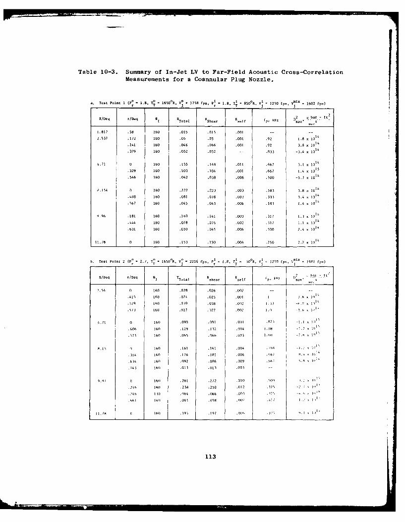
Table 10-3. Summary of In-Jet LV to Far-Field Acoustic Cross-CorrelationMeasurements for a Coannular Plug Nozzle.
a. Test Point 1 (Po 1.8, TOT - 16500R, V
0 - 1758 fps, P 1.8 ix..e .5 Is 62Ea
1.8 T60R o 78fpp 850OR, V 1250 fps, Vmi 1602 fps)
Tetot__ (r __ .8, T__ - j r " 8 T j =
j
X/Deq r/Deq G I Total RRShear Iself fp, kHz D2 w bar - ft2
max '
1.812 .58 160 .015 .015 .001 ....
2.537 .172 160 .05 .05 .001 .92 1.8 x 10¹⁴
.241 160 .046 .046 .001 .92 3.8 x 10¹⁴
.379 160 .052 .052 -- .833 -3.4 x I014
4.71 0 160 .155 .148 .011 .667 3.1 x l14
.329 160 .103 .104 .001 .667 1.4 x 10¹⁵
.546 160 .042 .038 .006 .500 -5.7 x 10¹⁴
R.154 0 160 .222 .223 .003 .583 3.8 x 10¹⁴
.408 160 .081 .078 .003 .333 3.4 x 10¹⁴
.567 160 .045 .043 .006 .583 1.4 x 10¹⁴
Q.96 .181 160 .140 .141 .003 .317 1.3 x 10¹⁴
.444 160 .078 .076 .002 .317 1.1 x 10¹⁴
.631 160 .050 .045 .006 .500 2.4 x 10¹⁴
11.78 0 160 .153 .150 .004 .250 2.2 x 10¹⁴
165008 * 221 oo i 20fpVix
-a 81f
h. Test Point 2 (P0
- 2.7, TT
1650R, V' - 2216 fps, r = 1.8, r 0'R, V- 1250 p, x - 1981 fp,)r~ T jT_ _ _ _
X/Deq r/Deq A T
Tt shear Rself f,, k)
2.54 0 160 .028 .026 .002 -- --
.415 160 .024 .025 .001 I 3.6 x 101 4
.529 160 .039 .038 .002 1.3 -,. x 111
.573 160 .027 .327 .002 1.01 -3.6 101'
4.11 0 160 .090 .091 .001 .871 -1.1 . W',
.406 160 .129 .132 .004 1.08 -7.2 0
.573 160 .065 .066 .005 1.0) -2 On In11
8.15 160 .161 .161 .004 .708 -l.. "
.314 160 .176 .181 .006 .66' .0 .1 4
.634 160 .092 .086 .009 .667 5. 1
.743 160 .013 .013 .003 --
9.41 0 160 .261 .272 .010 .W0)1 I.
.24f6 160 .238 .250 .012 .375 -2 2 I'
.246 130 .064 .066 .003 . k7'. - , , I
.h66 160 .065 .058 ,.007 .41i/ I ." 1' l'
11.7m 0 160 .195 .17 .006 .32.
113

0~0
41,
00
u M
4
o 0
(1
M4
Q)a)
4-.. 0iN INO

00
4
*0 0N0 04-
u IS
0 - 0
0 0 *0
0 4,
Its 0 ~ 0 *0~b 0
0VIA
m 4
4.1
In4
115

The result of Figure 10-15 illustrate features which exemplify most of
the measurements taken for this test series. The values of the measured in-
jet velocity to far-field acoustic normalized cross-correlations are of
significant magnitude (for this illustrativw case ,',l, t = 0.261) and the
actual measured correlation function shape is precise enough to ensure that
"real" regions of strong correlati ns are heing measured between the laser
and the acoustic microphone. Figures l()-lSa, h, c also show that the shear
portion (that is, the mean/turbulence velocity interaction field) dominates
the measured total cross-correlation tuIHt ion. The preeminence of the shear
cross-correlation was found to he truc for if0" ,of the measurements performed.
Figure l0-15d shows the second dIrivit ivw ricasrcments. This figure illus-
trates that the new statistical estimitor procedures developed (see Sections
7.0 and 8.0) together with the impr(o)Ivut i thc lser processor, were success-
fil*. The LV measured spectra of th total normalized cross-correlation function
and its second derivative are shown in Li gc I i S 10-15e and f. These spectra
results show that for the current measurement the dominant frequency is in
the lower frequency end of the spectrum and is fairly clear in the region of
importance. For RTotal the spectrum is quite good up to 3 kllz; thereafter,
the results are more than 25 dO down from the peak. ]2rr the spectrum of the
second derivative, after 15 dB down from the peak, the results indicate
further improvement could be made to define tie higher frequency region.
Figures 10-16a, b and c summarize some of the additional results obtained
from this series of measurementE. Figure 10-16a shows the axial variation of
the maximum value of the total in-jet velocity to far-field acoustic pressure
(at 6je t - 20') for the coannular plug nozzle for the two test conditions
tested; the results are for the centerline measurements onlv The values
of RTotal show a range between 0.029 to 0.261, depeding on axial location;
with the maximum occurring between 8-10 Deq. For test point 2 (the higher
velocity coannular plug nozzle test case), Figure 10-16b illustrates that
Rshear is generally 20 times greater than Rself for all of the measurements.
These new results are an up-date to previous results reported in Vols I andI of Reference 31.
Peak values of RTotaI were found along the cent irIinc. S,,c !B II- forvalues at other radial locations. Also see the Appendix.
116
Ad.
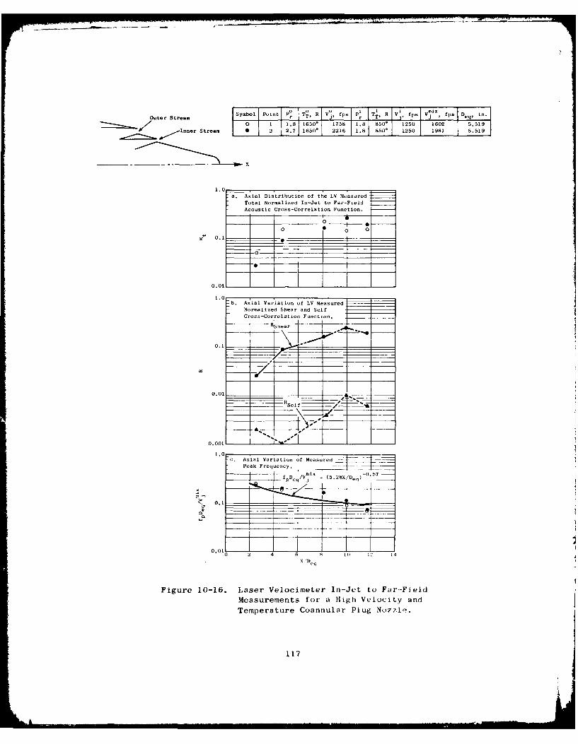
outer Strea. I~~O I T r A I T4 R _! p , "'n
0 1 1.81 1650:0 1758 1.8 8300 1250 1602 5.9InrStream, * 2.7 1 6500 2216 1.8 18500 1250 1981 51
a. Axial Distrihutior. of the LV Measured:T,,tal Normalized In-Jet to Far -FieldA co us tic Cross-Correlation Function.
0
0.1
1. .Axial Variation of LV MeasuredNornalized Shear and SelfCross-Correlation Function.
R Shear
0.01
-R
0.00: 1__
1. c. Axial Variation of Measu redPeak Frequency.n
a fpDeq/V"' (5.28X/Deq,-.5
0.1 _ _ _ __ _ _
000 2 4 6 ~ C i
Figure 10-16. Laser Velocimeter In-Jet to Far-Field
Measurements for a High Velocity and
Temperature Coannular Plug Nozzl-x.
117
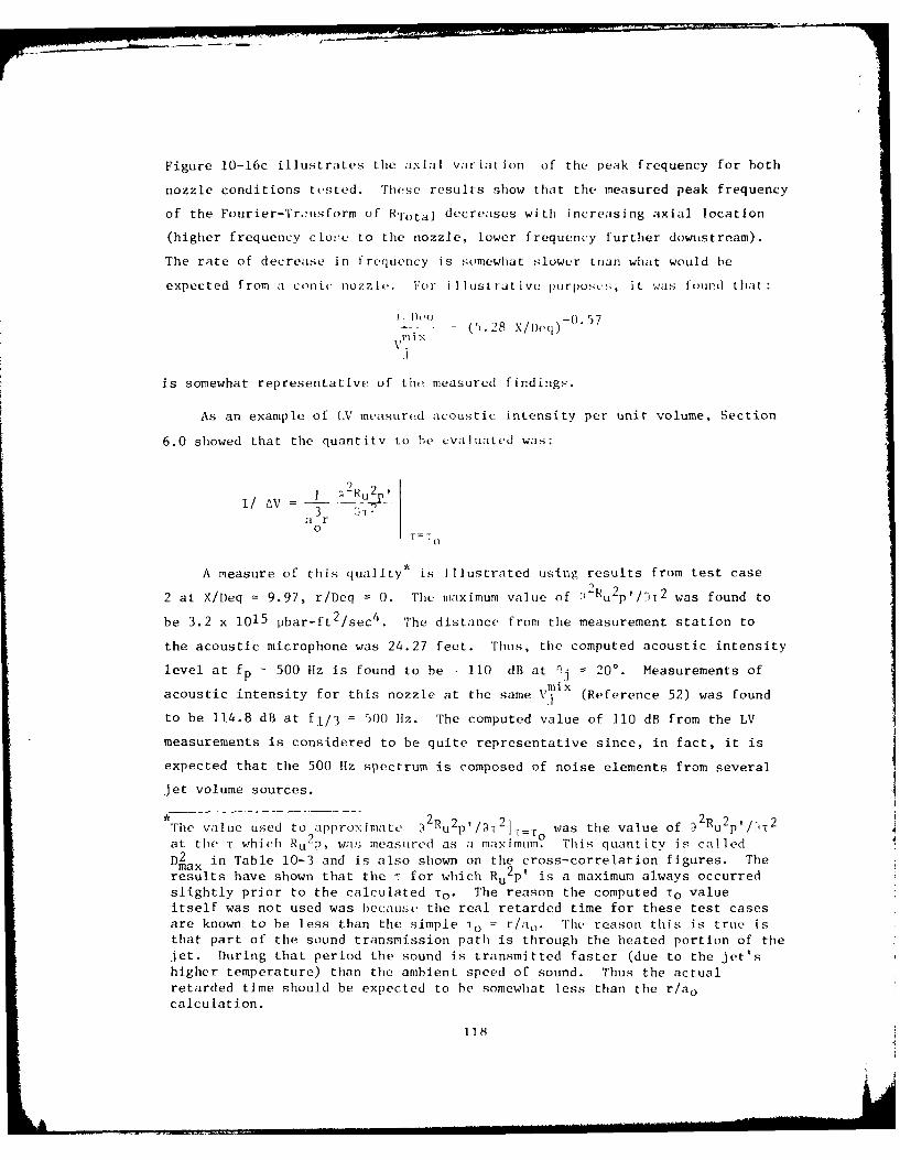
Figure 10-16c illustrates the axial var iat ion of the peak frequency for both
nozzle conditions tested. These results show that the measured peak frequency
of the Fourier-Tronsform of HRota] decreases with increasing axial location
(higher frequency clo!e to the nozzle, lower frequency further downstream).
The rate of decrease in frequency is somewhat slower tnan what would be
expected from a conic nozzle. For illustrative plirposcs, it was foUnd that:
k I 'hq -0.57.. (.28 X/Deq)
is somewhat representative of tho measured findings.
As an example of LV measured acoustic intensity per unit volume, Section
6.0 showed that the quantitv to be evaluated was:
I/ AV = R3 <E
a r0 T = T o
A measure of this quality* is illustrated using results from test case
2 at X/Deq = 9.97, r/Deq = 0. The maximum value of "'4 R 2 p'/ 5 1 2 was found to
be 3.2 x 10¹⁵ pbar-ft 2 /sec 4 . The distance from the measurement station to
the acoustic microphone was 24.27 feet. Thus, the computed acoustic intensity
level at fp - 500 Hz is found to be - 110 dB at Oj = 20'. Measurements of
acoustic intensity for this nozzle at the same V 1ix (Reference 52) was foundJ
to be 114.8 dB at fl/ 3 = 500 Hz. The computed value of 110 dB from the LV
measurements is considered to be quite representative since, in fact, it is
expected that the 500 Hz spectrum is composed of noise elements from several
jet volume sources.
•1 2u2p 2R u 2 p /,2
The value used to approximate /U2pIT ro was the value of '/R-u 2at the T which Ru2p .was measured as a maximum. This quantity is calledD2 in Table 10-3 and is also shown on the cross-correlation figures. Themaxresults have shown that the T for which Ru 2p' is a maximum always occurred
slightly prior to the calculated To . The reason the computed To valueitself was not used was because the real retarded time for these test cases
are known to be less than the simple To = r/ao. The reason this is true is
that part of the sound transmission path is through the heated portion of thejet. During that period the sound is transmitted faster (due to the jet's
higher temperature) than the ambient speed of sound. Thus the actual
retarded time should be expected to be somewhat less than the r/a o
calculation.
118

The results illustrated above have shown that the laser velocimeter
techniques developed over the past several years can be useful as a diagnostic
tool for better understanding realistic jet nozzle turbulent and acoustic
features at typical engine velocity and temperature conditions. The results
have illustrated that important aerodynamic source term results, such as
turbulent length scale, convection velocity, turbulent and mean velocity, can
be measured for complex nozzle flow fields and that cross-correlation
measurements between the point velocity field and the far-field acoustic
radiation field have shown strong regions of correlation heretofore not
measured. These results are considered to be quite encouraging for future
investigations in nozzle noise and aerostructure characteristics of high
velocity and temperature jets.
Some additional remarks regarding the cross-correlation function shouldbe noted. As shown in Figure 10-15c the measured normalized cross-correlation
function is somewhat symmetrical with a negative peak. This shape was not
always the same for all meaourements. For certain locations, the cross-
correlation coefficient was symmetric with a positive peak. An example of
this type of correlation function is given in the Appendix (X/Deq = 9.97,
r/Deq = 0.246). The reason for such a contrasting difference between the
two cross-correlation functions is expected to be related to some physical
flow phenomenon which needs further evaluation and explanation.
119

11.0 CONCLUDING REMARKS AND RECOMMENDATIONS
11.1 CONCLUDING REMARKS
The studies and discussions contained in this report include a number of
unique and modern concepts for laser velocimeter signal processing and data
handling and reduction associated with performing real-time velocity and
cross-correlation measurements in realistic jet exhaust nozzle flows. The
introduction of the filter bank approach for LV signal processing and the
use of quantized product factoring in the LV data handling cycle have enabled
a time improvement of a factor of 90 in LV data acquisition in the most
severe type of velocity and temperature conditions.
A series of two-point space-time velocity measurements for determining
a jet's turbulent length scale and convection speed was successfully per-
formed for a baseline conic nozzle and for an inverted velocity and tempera-
ture flow coannular plug nozzle. Experiments were performed in jet exhausts
of 2200 fps and 16500 R. Additionally, a series of in-jet velocity to far-
field acoustic cross-correlation measurements was performed on a coannular
plug nozzle at sonic and supersonic heated flow conditions. Measurements of
this type have not been previously performed. The results of the studies
performed to date indicate that the LV technology is at hand to begin sys-
tematic aerodynamic and acoustic noise source type experiments for high tem-
perature subsonic and supersonic exhaust jets.
Some of the results obtained from the recent cross-correlation measure-
ments are:
" For a simple conic nozzle, there exists a radial and axial vari-ation of turbulent length scale and convection speed throughout thejet.
" For the conic nozzle, it was found that not a great difference be-tween ambient and heated jet flow existed for length scale andconvection speed.
* For the inverted flow, coannular plug nozzle tested, an axial andradial variation of length scale and convection speed also was
found. The physical picture that emerges is that the smaller
120

turbulent eddies of the exhaust plume are convecting along thecenter line, the larger eddies are at a 70% Umax stream-line onthe outside of the jet, and intermediate size eddies are convectingalong of the Umax stream line.
" The convection velocities for the coannular plug nozzle were foundto be highest close to the nozzle and to gradually decay in speedwith increasing axial location. The centerline and Umax streamlineeddies convected the fastest, with the slower convecting eddieslocated at the 70% Umax streamline. Typical convection speedsranged as Vc = 0.4 - 1.0 Vcharacteristics.
" Regions of strong correlation were measured on the coannular plugnozzle where the LV velocity signal was cross-correlated with anacoustic microphone. Normalized cross-correlations of 0.26 wereobtained.
" For all tests performed, the shear turbulence aeroacoustic correla-tion function dominated. The shear cross-correlation coefficientwas at least a factor of 20 greater than the self-turbulence aero-acoustic cross-correlation function.
" The peak frequence of the cross-correlation function varied as
f Deqmix = (5.28 X/Deq) -0.57ixJ
Thus, the classic notion of high frequency noise generation occurring
close to the coannular plug nozzle and low frequency noise occurring down-
stream was verified.
11.2 RECOMMENDATIONS FOR FUTURE WORK
1. The development of the laser velocimeter as a viable, economicaljet noise diagnostic tool has been demonstrated. It is recommendedthat a series of systematic and detailed measurements be performedto better define the turbulent structure of jets, convection speedand scale of turbulence. The initial nozzles recommended for studyare: 1) the conic nozzle, 2) coaxial coplanar, 3) coannular plugnozzle. Experiments should be performed at subsonic and supersonicconditions. In addition, in-jet velocity to far-field acousticpressure cross-correlation measurements on the above three nozzlesshould be performed to quantify the regions of strong correlationfor these nozzles. Further extension of the methods developed here
to partial coherence techniques is also recommended.
121

2. Application of some of the more modern theoretical acoustic model-ing techniques toward additional definition and clarification ofthe aerodynamic source terms should be performed.
3. Although great strides have been made in the improvements of the LVprocessor and LV head, additional advancements will be forthcomingwith the applications in large scale integrated circuits (micro-processors). Development as a Fast Fourier transform type LVprocessor with a microprocessor approach is recommended.
4. Expansion of the LV arrangement to include a multivector outputarrangement is desirable.
122
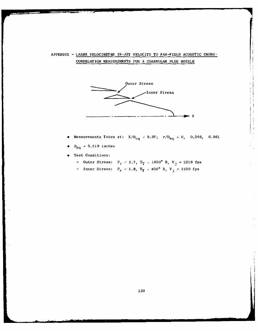
APPENDIX -LASER VELOCIMETER IN-JET VELOCITY TO FAR-FIELD ACOUSTIC CROSS-
CORRELAT ION MEASUREMENTS FOR A COANNULAR PLUG NOZZLE
Outer Stream
Inner Stream
_ _ _ _ -_ _ _ _ _ _ _ _ -X
* Measurements Taken at: X/Deq 9.97; r/D eq 0,l 0.246, 0.661
* De = 5.519 inches
* Test Conditions:
- Outer Stream: Pr =2.7, TT = 16500 R, V3 2216 fps
- Inner Stream: Pr =1.8, TT = 8500 R, V. 1250 fps
123
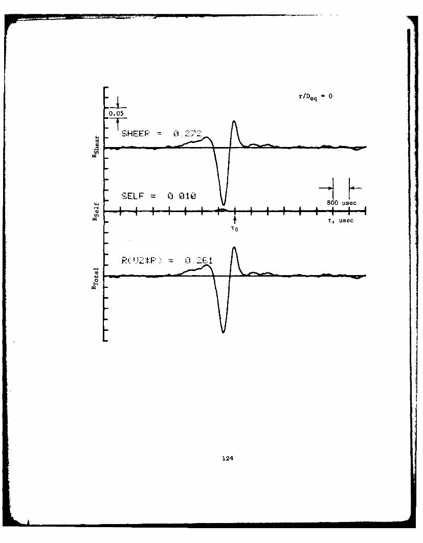
r/Deq 0
0.05
t 7 HEEF 0 1;'
JELF 0 i 1HH800 pisec
T, lisec
0
124

r/Deq =0
0.05
E-4
c'Je
0
125

eq
5 5dB
Si E, ~2 'f, kHz
Ct
126

0.05 r/Deq 0.246
--
S- IiE E P .5
SEELF 0 0 12H 4- 800 iisec
t T, lisec
F:'. I)2j..' 023:
E0
127

P~:IJIP:a iir/D eq =0.246
fV
p 800 psec
9 T
128
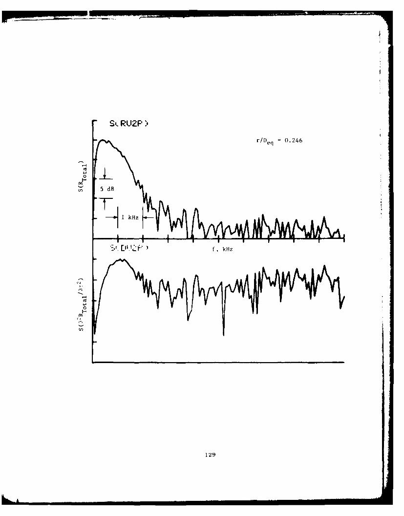
SiC RU2F)
rIDeq 0.246
5
[-wIkHz ll', AIA &A I
(-'H4I v
f ,--.i
'129

r/Deq 0.661
0. 05
.E LF 0 00071 H800 1isec
4- 1 4 1 1- +i i jh
t T, p'sec
TO0
130

rID = 0.661
0.05
0
800 1 sec
O~1P = I E 15R A, i sec
D2 /5max
1'31

S( RZP)rlDeq =0.661
0
5 dB
T -~jikHz[-
f H
~J
132
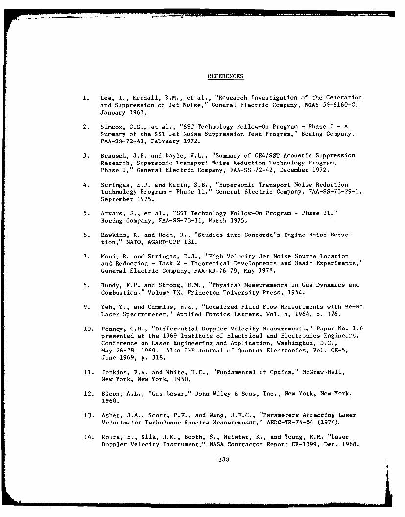
REFERENCES
1. Lee, R., Kendall, R.M., et al., "Research Investigation of the Generationand Suppression of Jet Noise," General Electric Company, NOAS 59-6160-C,January 1961.
2. Simcox, C.D., et al., "SST Technology Follow-On Program - Phase I - ASummary of the SST Jet Noise Suppression Test Program," Boeing Company,FAA-SS-72-41, February 1972.
3. Brausch, J.F. and Doyle, V.L., "Summary of GE4/SST Acoustic SuppressionResearch, Supersonic Transport Noise Reduction Technology Program,Phase I," General Electric Company, FAA-SS-72-42, December 1972.
4. Stringas, E.J. and Kazin, S.B., "Supersonic Transport Noise ReductionTechnology Program - Phase II," General Electric Company, FAA-SS-73-29-1,
September 1975.
5. Atvars, J., et al., "SST Technology Follow-On Program - Phase II,"Boeing Company, FAA-SS-73-11, March 1975.
6. Hawkins, R. and Hoch, R., "Studies into Concorde's Engine Noise Reduc-
tion," NATO, AGARD-CPP-131.
7. Mani, R. and Stringas, E.J., "High Velocity Jet Noise Source Locationand Reduction - Task 2 - Theoretical Developments and Basic Experiments,"General Electric Company, FAA-RD-76-79, May 1978.
8. Bundy, F.P. and Strong, H.M., "Physical Measurements in Gas Dynamics andCombustion," Volume IX, Princeton University Press, 1954.
9. Yeh, Y., and Cummins, H.Z., "Localized Fluid Flow Measurements with He-NeLaser Spectrometer," Applied Physics Letters, Vol. 4, 1964, p. 176.
10. Penney, C.M., "Differential Doppler Velocity Measurements," Paper No. 1.6
presented at the 1969 Institute of Electrical and Electronics Engineers,Conference on Laser Engineering and Application, Washington, D.C.,May 26-28, 1969. Also lEE Journal of Quantum Electronics, Vol. QE-5,
June 1969, p. 318.
11. Jenkins, F.A. and White, H.E., "Fundamental of Optics," McGraw-Hall,New York, New York, 1950.
12. Bloom, A.L., "Gas Laser," John Wiley & Sons, Inc., New York, New York,1968.
13. Asher, J.A., Scott, P.F., and Wang, J.F.C., "Parameters Affecting LaserVelocimeter Turbulence Spectra Measuremnent," AEDC-TR-74-54 (1974).
14. Rolfe, E., Silk, J.K., Booth, S., Meister, K., and Young, R.M. "LaserDoppler Velocity Instrument," NASA Contractor Report CR-1199, Dec. 1968.
133

15. Lennert, A.E., Brayton, D.B., Crosswy, F.L., et al., "Summary Reportof the Development of a Laser Velocimeter to be used in AEDC WindTunnels," ARO, Inc., Report No. AEDC-TR-70-101, July, 1970.
16. TSI, Inc. Catalog 900-477 "Laser Anemometer Systems:' St. Paul, Minn.,1977.
17. DISA Electronics Catalog 5205E "Laser Doppler Anemometer Equipment,"Franklin Lakes, N.J., 1977.
18. Jones, W.B., "Laser Fluid Velocity Sensor," Paper No. 2-8-82 Symposiumon Flow, Pittsburg, Pa., sponsored by AIAA, AlP, and NBS, May, 1971.
19. Pike, E.R., "Photon Correlation Methods," Proceedings of the SecondInternational Workshop on Laser Velocimetry, Purdue University,March 27-29, 1974.
20. Kalb, H.T., and Cline, V.A. "New Technique in the Processing and Handlingof Laser Velocimeter Burst Data," pp. 708-711, Review of ScientificInstruments, Vol. 47, No. 6, June 1976.
21. Diermendjian, Closen, and Viegee, Journal of the Optical Society ofAmerica, 51, 621 (1961).
22. Engstrom, R.W., et al., Photomultiplier Manual, Chapter "StatisticalFluctuation and Noise,' RCA Corporation, Harrison, N.J., 1970.
23. Benzakein, M.J. and Knott, P.R., "Supersonic Jet Exhaust Noise," AirForce Aero Propulsion Lab, AFAPL-TR-72-52, July, 1972.
24. Wisler, D.C., and Mossey, P.W. "Practical Applications of LV Systems toAero Engine Research and Development," AGARD Lecture Series No. 90,"Laser Optical Measurement Methods for Aero Engine Research and Develop-ment," August - September, 1977.
25. Asher, J.A., "Laser Doppler Velocimeter System Development and Testing,"GE Report 72CRD295, also published in AIAA Progress in Astronautics andAeronautics, Vol. 34.
26. Whalen, A., "Detection of Signals in Noise," Academic Press, 1965.
27. Lighthill, M.J., 1952 Proceedings of the Royal Society A211, 564-587,"On Sound Generated Aerodynamically I. General Theory."
28. Lighthill, M.J., 1954 Proceedings of the Royal Society A222, 1-32."On Sound Generated Aerodynamically II. Turbulence as a Source ofSound."
29. Knott, P.R., Benzakein, M.J., "Analytical and Experimental Supersonic JetExhaust Noise Research," AIAA 73-188 (1973).
134

30. Knott, P.R. et al., "Supersonic Jet Exhaust Noise Investigation,"AFAPL-TR-74-25 (June 1974).
31. Knott, P.R. et al., "Supersonic Jet Exhaust Noise Investigation,"Volume I, II, III and IV, AFAPL-TR-76-68 (July 1976).
32. Mani, R., "The Influence of Jet Flow on Jet Noise - Part I and II,"Journal of Fluid Mechanics - Vol. 73, 1976, pp 753-793.
33. Balsa, T.F., "Fluid Shielding of Low Frequency Convected Sources byArbitrary Jet," Journal of Fluid Mechanics, Vol. 70, 1975, pp 17-36.
34. Ribner, H.S., "The Generation of Sound by Turbulent Jets," Advances inApplied Mechanics, Vol. 3, Academic Press, New York, 1964, pp. 103-182.
35. Lee, H.K., "Correlation of Noise and Flow of a Jet," UTIAS Rep. 168,Aug. 1971.
36. Lee, H.K. and Ribner, H.S., "Direct Correlation of Noise and Flow of a Jet,"AIAA 72-640.
37. Chu, W.T., "Turbulence Measurements Relevant to Jet Noise," UTIAS Report119 (Nov. 1966).
38. Proudman, I., "The Generation of Noise by Isotropic Turbulence," Proc. Roy.Soc. A214, pp 119-132 (1952).
39. Clark, P.J.F. and Ribner, H.S., "Direct Correlation of Fluctuating Liftand Radiated Sound for an Airfoil in Turbulent Flow," Jour. of theAcoustical Society of America, Vol. 46, No. 3 (Part 2), 1969, pp 802-805.
40. Siddon, T.E., "Surface Dipole Strength for Flow Past Airfoils," Journ. ofthe Acoustical Society of America, Vol. 48, No. 1 (Part 1), 1970.
41. Meecham, W.C., and Forel, G.W., "Acoustic Radiation from Isotropic Turbu-lence," Journ. of the Acoustical Society of America, Vol. 30 No. 4, 1958,pp 318-322.
42. Seiner, J.M. and Reethof, G., "On the Distribution of Source Coherency inSubsonic Jets," AIAA 74-4 (1974).
43. Bendat, J.S. and Pierson, A., Random Data: Measurement & Analysis Pro-cedures; Wiley; 1971; Sec. 6.3.
44. Enochsen, L. and Otnes, R. "Programming and Analysis for Digital TimeSeries Data," U.S. D.O.D., SU*-3, 1968 pg 215.
45. Hahn, G. and Shapiro, S., Statistical Models in Engineering, Wiley, 1967,Sec. 2-9.
135d

46. Scott, P.F., "The Auto-Correlation Functions and Spectra of a Signalthat has Been Randomly Sampled," Conference Record, IEEE76 CH1067-8.
ASSP, pp 296-299.
47. Scott, P.F., "Distortion and Estimation of the Auto-Correlation Functionand Spectrum of a Randomly Sampled Signal," General Electric, 76CR180,Class I, 1976.
48. Hinze, J.O., Turbulence; McGraw-Hill, 1959, pgs. 49-51.
49. Fletcher, R. and Reeves, C.M., "Function Minimization by ConjugateGradients."
50. Scott, P., "The Theory and Implementation of LV Spectra Measurements,"International Workshop on Laser Velocimeters, 23 March 1974.
51. Knott, P.R., Scott, P., Mossey, P., "Noise Source Diagnostic Methodswith a Laser Velocimeter," 1977 Independent Research and DevelopmentTechnical Plan, Volume III, March 1977, R77AEG326.
52. Knott, P.R., Blozy, J.T., Staid, P.S., "Acoustic and PerformanceInvestigation of Coannular Plug Nozzle," NAS3-19777, May 1977.
136

DAT
FILM