fa.morganstanley.com methodology and asset allocation 59 - 62 key asset class risk considerations 63...
TRANSCRIPT
John and Jane Smith
January 04, 2016
LifeView® Financial Goal Analysis
Prepared by:
John Advisor, CFP®Financial AdvisorSAMPLE

Table Of Contents
IMPORTANT DISCLOSURE INFORMATION 1 - 4
Summary of Goals and Resources
Personal Information and Summary of Financial Goals 5 - 6
Net Worth Summary - All Resources 7
Net Worth Detail - All Resources 8 - 9
Resources Summary 10 - 11
Current Portfolio Allocation 12 - 13
Target Band 14
Results
What If Worksheet 15 - 20
Worksheet Detail - Combined Details 21 - 26
Worksheet Detail - Health Care Expense Schedule 27 - 29
Worksheet Detail - Retirement Distribution Cash Flow Chart 30 - 38
Worksheet Detail - Inside the Numbers Final Result 39
Worksheet Detail - Bear Market Test 40
Worksheet Detail - Special Asset Test 41
Worksheet Detail - Portfolio Probability Matrix 42
Worksheet Detail - Allocation Comparison 43 - 44
Worksheet Detail - Social Security Maximization 45 - 46
Employer Stock Plans
Stock Options 47 - 48
Stock Options Summary 49 - 51
Appendix
Risk Assessment 52 - 54
Explain Real Returns 55
Tax and Inflation Assumptions 56
IMPORTANT DISCLOSURE INFORMATION 57 - 58
Return Methodology and Asset Allocation 59 - 62
Key Asset Class Risk Considerations 63 - 64
Glossary of Terms 65 - 69
SAMPLE
IMPORTANT DISCLOSURE INFORMATION
01/04/2016
Prepared for : John and Jane Smith Prepared by: John Advisor
Page 1 of 69
Information that you provided about your assets, financial goals, and personal situation arekey assumptions for the calculations and projections in this Report. Please review all theinformation thoroughly to ensure that it is correct and complete. In particular, please reviewthe Report sections titled "Personal Information and Summary of Financial Goals", CurrentPortfolio Allocation", and "Tax and Inflation Assumptions" to verify the accuracy of theseassumptions. If any of the assumptions are incorrect, you should notify your FinancialAdvisor. Even small changes in assumptions can have a substantial impact on the resultsshown in this Report. The information provided by you should be reviewed periodically andupdated when either the information or your circumstances change. Morgan Stanley has noresponsibility and is under no obligation to monitor or update this Report in the futureunless expressly engaged by you to do so at that time.
Information Provided by You
Every individual’s financial circumstances, needs and risk tolerances are different. ThisLifeView® Financial Goal Analysis (the "Report") is based on the information you providedto us, the assumptions you have asked us to make and the other assumptions indicatedherein as of the date of the Report. It is not an official account statement. The purpose oftaking the time to organize your financial life is to gain better control of your financialfuture. This Report should be considered a working document that can assist you with thisobjective. You should carefully review the information and suggestions found in this Reportand then decide on future steps.
Asset Allocation Information
LifeView Goal Analysis Assumptions and Limitations
LifeView Goal Analysis is powered by MoneyGuidePro®
IMPORTANT: The projections or other information generated by LifeView® GoalAnalysis regarding the likelihood of various investment outcomes (including anyassumed rates of return) are hypothetical in nature, do not reflect actualinvestment results, and are not guarantees of future results.
Any asset allocation information presented herein, which may take into account your assetsin one or more Employee Retirement Income Security Act of 1974, as amended("ERISA")-covered employee benefit plans and/or one or more individual retirementaccounts, is for general asset allocation education and information purposes only, andshould not be viewed as fiduciary investment advice or specific recommendations withrespect to any particular investment or asset allocation mix under the Investment AdvisersAct of 1940 as amended, ERISA, the Internal Revenue Code or any other applicable law. Inapplying any particular asset allocation model to your individual circumstances, you shouldconsider your other assets, income and investments, in addition to any interest(s) you mayhave in ERISA-covered employee benefit plans or individual retirement accounts. Thus, it isvery important for you to insure that you review this Report to make sure that it includes allof your assets, income and investments.
Assumptions and Limitations
LifeView Goal Analysis offers several methods of calculating results, each of which providesone outcome from a wide range of possible outcomes. LifeView Goal Analysis does notpurport to recommend or implement an investment strategy. Financial forecasts, rates ofreturn, risk, inflation, and other assumptions may be used as the basis for illustrations inLifeView Goal Analysis. They should not be considered a guarantee of future performanceor a guarantee of achieving overall financial objectives. All results use simplifying estimatesand assumptions that are not tailored to your specific circumstances. No Report has theability to accurately predict the future, eliminate risk or guarantee investment results. Asinvestment returns, inflation, taxes, and other economic conditions vary from the LifeViewGoal Analysis assumptions, your actual results will vary (perhaps significantly) from thosepresented in this Report.
The assumed return rates in LifeView Goal Analysis are not reflective of any specificinvestment and do not include any fees or expenses that may be incurred by investing inspecific products. The actual returns of a specific investment may be more or less than thereturns used in LifeView Goal Analysis. The return assumptions are based on historic rates ofreturn of securities indices which serve as proxies for the broad asset classes. It is notpossible to directly invest in an index. Moreover, different forecasts may choose differentindices as a proxy for the same asset class, thus influencing the return of the asset class.LifeView Goal Analysis results may vary with each use and over time.
SAMPLE
IMPORTANT DISCLOSURE INFORMATION
01/04/2016
Prepared for : John and Jane Smith Prepared by: John Advisor
Page 2 of 69
Morgan Stanley cannot give any assurances that any estimates, assumptions orother aspects of the analyses will prove correct. They are subject to actual knownand unknown risks, uncertainties and other factors that could cause actual resultsto differ materially from those shown.
These analyses speak only as of the date of this Report. Morgan Stanley expresslydisclaims any obligation or undertaking to update or revise any statement or otherinformation contained herein to reflect any change in past results, futureexpectations or circumstances upon which that statement or other information isbased.
Rate of Return Methodology
The analysis contained in the Report is conducted using the Morgan Stanley WealthManagement Global Investment Committee’s Secular Return Estimates (“GIC Estimate”).GIC Estimate approved returns are generated based on proprietary formulas which includestudying historical return averages of the broad market indices and making strategicadjustments for more recent market conditions and other factors deemed relevant by theforecaster. The Return Methodology and Asset Allocation sections include a description ofthe return methodology that has been used to prepare this Report. The methodology shouldbe carefully considered in evaluating the results presented to you.
LifeView Goal Analysis is powered by MoneyGuidePro®
The return assumptions used in this Report are estimates based on average annual returnsfor the index used as a proxy for each asset class. The portfolio returns are calculated byweighting individual return assumptions for each asset class according to your portfolioallocation. During the preparation of these analyses, your Morgan Stanley Financial Advisormay have refined the asset allocation strategy to develop a strategy which optimizes thepotential returns that could be achieved with the appropriate level of risk that you would bewilling to assume. Asset classes not included may have characteristics similar or superior tothose being analyzed.
Hypothetical performance results have inherent limitations. There are frequently largedifferences between hypothetical and actual performance results subsequently achieved byany particular asset allocation or trading strategy. Hypothetical performance results do notrepresent actual trading and are generally designed with the benefit of hindsight. Theycannot account for all factors associated with risk, including the impact of financial risk inactual trading or the ability to withstand losses or to adhere to a particular trading strategyin the face of trading losses. There are numerous other factors related to the markets ingeneral or to the implementation of any specific trading strategy that cannot be fullyaccounted for in the preparation of hypothetical performance results and all of which canadversely affect actual trading results.
Monte Carlo simulations are used to show how variations in rates of return each year canaffect your results. A Monte Carlo simulation calculates the results of your Plan by runningit many times, each time using a different sequence of returns. Some sequences of returnswill give you better results, and some will give you worse results. These multiple trialsprovide a range of possible results, some successful (you would have met all your goals) andsome unsuccessful (you would not have met all your goals). The percentage of trials thatwere successful is shown as the probability that your Plan, with all its underlyingassumptions, could be successful. In LifeView Goal Analysis, this is the Probability ofSuccess. Analogously, the percentage of trials that were unsuccessful is shown as theProbability of Failure. The Results Using Monte Carlo Simulations indicate the likelihoodthat an event may occur as well as the likelihood that it may not occur. In analyzing thisinformation, please note that the analysis does not take into account actual marketconditions, which may severely affect the outcome of your goals over the long-term.
Results Using Monte Carlo Simulations
SAMPLE
IMPORTANT DISCLOSURE INFORMATION
01/04/2016
Prepared for : John and Jane Smith Prepared by: John Advisor
Page 3 of 69
IMPORTANT NOTES AND DISCLOSURES FROM MORGAN STANLEY
Morgan Stanley provides its existing and prospective brokerage customers with a number offinancial tools that produce certain reports to assist customers in managing their wealth andassets. These tools generate reports that include this Report. This Report is generated byusing a computer software program developed by MoneyGuidePro, a third party softwareprovider. Results may vary with each use of the software and over time. Enhancementsand changes to the software may be made in the future. Morgan Stanley is not responsiblefor the accuracy of the assumptions made in the Report, or the calculations in the analyses.Future Reports may contain information capabilities and other content that is moreexpansive or otherwise different from the content of this Report.
This Report creates a brokerage relationship among you, your Financial Advisor and MorganStanley. You should understand the differences between a brokerage and advisoryrelationship. When providing you brokerage services, our legal obligations to you aregoverned by the Securities Act of 1933, the Securities Exchange Act of 1934, the rules ofself-regulatory organizations such as the Financial Industry Regulatory Authority (FINRA),and state securities laws, where applicable. When providing you advisory services, our legalobligations to you are governed by the Investment Advisers Act and applicable statesecurities laws. These latter advisory obligations govern our conduct and disclosurerequirements, creating a legal standard which is referred to as a “fiduciary” duty to you.Please ask your Financial Advisor questions to make sure you understand your rights and ourobligations to you, including the extent of our obligations to disclose conflicts of interestand to act in your best interest. For additional answers to questions about the differencesbetween our advisory and brokerage services, please visit our web site athttp://www.morganstanley.com/ourcommitment/ or contact us at 866-866-7426.
Morgan Stanley is both a registered broker-dealer and investment adviser and its FinancialAdvisors act in dual capacities as broker-dealer and investment advisory representatives.Many Morgan Stanley Financial Advisors may use the designation Certified Financial Planneror "CFP," a certification mark owned by the Certified Financial Planner Board of Standards,Inc. Each of these Financial Advisors also is licensed to act as a broker-dealer representativeon behalf of Morgan Stanley. When any of these Financial Advisors assists clients byproviding them a LifeView® Financial Plan, he/she is doing so as a CFP and investmentadvisory representative of Morgan Stanley. However, in providing other services tocustomers, such as assisting customers in implementing a Financial Plan once it has beendelivered, providing financial tools/reports to customers, or effecting transactions for thecustomer's brokerage account, the Financial Advisor carrying a CFP designation is onlyacting as a broker-dealer representative unless the Financial Advisor and client have enteredinto a written agreement that creates an investment advisory relationship.
This Report is not a financial plan. A financial plan generally seeks to address a widespectrum of your long-term financial needs, and can include recommendations aboutinsurance, savings, tax and estate planning, and investments, taking into consideration yourgoals and situation, including anticipated retirement or other employee benefits. MorganStanley will only prepare a financial plan at your specific request using Morgan Stanleyapproved financial planning software where you will enter into a written agreement with aFinancial Advisor, such as Morgan Stanley LifeView® Advisor. If you would like to have afinancial plan prepared for you, please consult with your Financial Advisor.
This Report does not constitute an offer to buy, sell, or recommend any particularinvestment or asset, nor does it recommend that you engage in any particular investment,manager or trading strategy. It reflects only allocations among broad asset classes. Allinvestments have risks. The decisions as to when and how to invest are solely yourresponsibility.
By providing you this Report, neither Morgan Stanley nor your Financial Advisorare acting as a fiduciary for purposes of the Investment Advisers Act of 1940, asamended (the “Investment Advisers Act”), ERISA or section 4975 of the Code withrespect to any ERISA-covered employee benefit plan or any individual retirementaccount in either the planning, execution or provision of this analysis. Unlessotherwise provided in a written agreement between you and Morgan Stanley,Morgan Stanley, its affiliates and their respective employees, agents andrepresentatives, including your Financial Advisor, (a) do not have discretionaryauthority or control with respect to the assets in any ERISA-covered employeebenefit plan or any individual retirement account included in this Report, (b) willnot be deemed an "investment manager" as defined under ERISA, or otherwisehave the authority or responsibility to act as a "fiduciary" (as defined under ERISA,the Investment Advisers Act or other applicable law) with respect to such assets,and (c) will not provide "investment advice," as defined by ERISA and/or section4975 of the Internal Revenue Code, as amended, with respect to such assets.
Please keep in mind that Morgan Stanley is not a tax or legal advisor and this Report doesnot constitute tax, legal or accounting advice. You should discuss any tax and legalinformation outlined in this document with your accounting, tax and legal advisors prior totaking action. Your Morgan Stanley Financial Advisor can work with you and these advisorsto answer your questions and, if you choose, help you implement the options you decideupon. There is no requirement, however, that you implement any strategies at all. Inaddition, you are not obligated to implement any options shown in this Report or tootherwise conduct business through Morgan Stanley or its affiliates.
Timing for implementing, monitoring and adjusting your strategies is a critical element inachieving your financial objectives. You are responsible for implementing, monitoring andperiodically reviewing and adjusting your investment strategies.
SAMPLE

IMPORTANT DISCLOSURE INFORMATION
01/04/2016
Prepared for : John and Jane Smith Prepared by: John Advisor
Page 4 of 69
IMPORTANT NOTES AND DISCLOSURES FROM MORGAN STANLEY (continued)
Powered by MoneyGuidePro® and MoneyGuidePro® are marks of PIEtech, Inc.
By accepting delivery of this Report, you are deemed to acknowledge and agree that:
1) you have reviewed and accept the information contained within this Report andunderstand the disclaimers, assumptions and methods included with it;
2) you believe that all information provided by you is complete and accurate to the best ofyour knowledge;
3) you recognize that all investments have risks; that performance and attainment offinancial objectives are not guaranteed; and that all estimates and assumed data, includingreturns, are included only for general education and do not represent a forecast of futureevents or results;
4) you understand that this Report was generated using a brokerage tool, is not a financialplan and created a brokerage (not advisory) relationship among you, your Financial Advisorand Morgan Stanley that governed the preparation of this Report and ended upon receiptof this Report;
6) you understand that Morgan Stanley is not a legal or tax advisor and that this Reportdoes not constitute tax, legal, or accounting advice.
© 2012 Morgan Stanley Smith Barney LLC. Member SIPC.
5) you understand that Morgan Stanley and your Financial Advisor are not fiduciaries underERISA or the Internal Revenue Code with respect to this Report or your use or our use (onyour behalf) of the software which generated this Report, or your IRA and retirement planaccounts unless otherwise provided in a written agreement between you and MorganStanley. The information in this Report is provided to you on the understanding that, forpurposes of ERISA and the Code, it is intended to be educational material, will not form aprimary basis for any investment decision made by you or on your behalf, and will not beviewed for ERISA or Code purposes as fiduciary investment advice or specificrecommendations with respect to asset allocation or any particular investment, and that(unless otherwise provided in a written agreement) you remain solely responsible for yourassets and all investment decisions with respect to your assets; andSAMPLE

Summary of Goals and Resources
SAMPLE
Personal Information and Summary of Financial Goals
01/04/2016
Prepared for : John and Jane Smith Prepared by: John Advisor
Page 5 of 69
See IMPORTANT DISCLOSURE INFORMATION at the beginning and at the back of this document for explanations of assumptions, limitations, and methodologies.
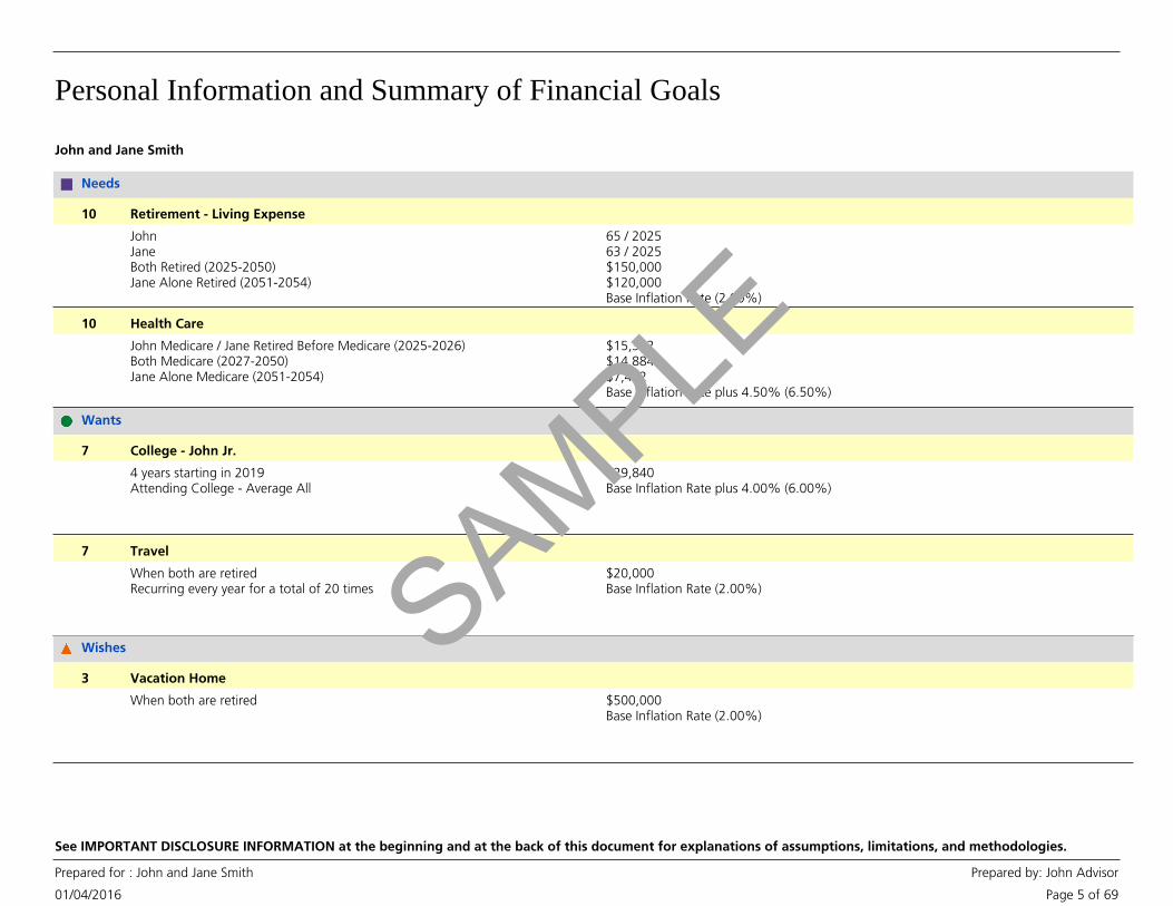
John and Jane Smith
Needs
Retirement - Living Expense10
JohnJaneBoth Retired (2025-2050)Jane Alone Retired (2051-2054)
65 / 202563 / 2025$150,000$120,000Base Inflation Rate (2.00%)
Health Care10
John Medicare / Jane Retired Before Medicare (2025-2026)Both Medicare (2027-2050)Jane Alone Medicare (2051-2054)
$15,302$14,884$7,442Base Inflation Rate plus 4.50% (6.50%)
Wants
College - John Jr.7
4 years starting in 2019Attending College - Average All
$29,840Base Inflation Rate plus 4.00% (6.00%)
Travel7
When both are retiredRecurring every year for a total of 20 times
$20,000Base Inflation Rate (2.00%)
Wishes
Vacation Home3
When both are retired $500,000Base Inflation Rate (2.00%)
SAMPLE

Personal Information and Summary of Financial Goals
01/04/2016
Prepared for : John and Jane Smith Prepared by: John Advisor
Page 6 of 69
See IMPORTANT DISCLOSURE INFORMATION at the beginning and at the back of this document for explanations of assumptions, limitations, and methodologies.
Personal Information
John
Male - born 05/22/1960, age 55
Jane
Female - born 08/07/1962, age 53
Married, US Citizens living in NY
Employed - $150,000
Employed - $150,000
• This section lists the Personal and Financial Goal information you provided, which willbe used to create your Report. It is important that it is accurate and complete.
Participant Name Date of Birth Age Relationship
John Jr. 02/01/2001 14 Child
SAMPLE
Net Worth Summary - All Resources
01/04/2016
Prepared for : John and Jane Smith Prepared by: John Advisor
Page 7 of 69
See IMPORTANT DISCLOSURE INFORMATION at the beginning and at the back of this document for explanations of assumptions, limitations, and methodologies.
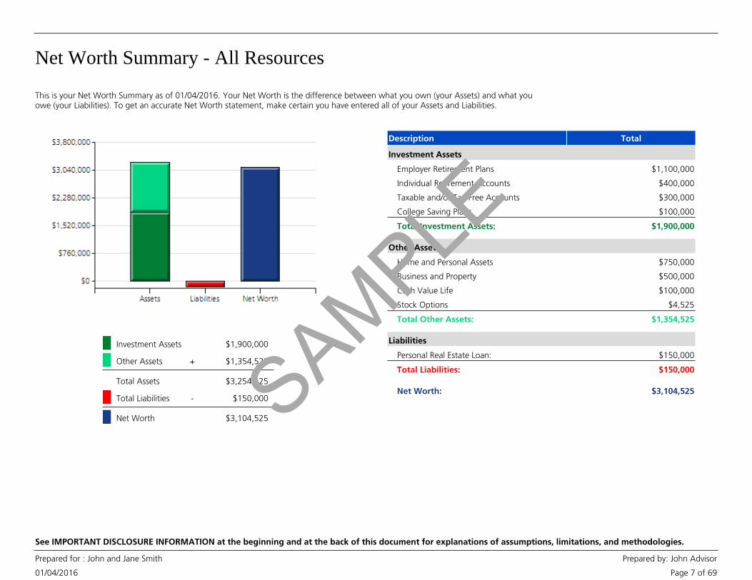
This is your Net Worth Summary as of 01/04/2016. Your Net Worth is the difference between what you own (your Assets) and what youowe (your Liabilities). To get an accurate Net Worth statement, make certain you have entered all of your Assets and Liabilities.
+ $1,354,525Other Assets
Investment Assets $1,900,000
Total Liabilities $150,000
Net Worth $3,104,525
$3,254,525Total Assets
-
Description Total
Investment Assets
Employer Retirement Plans $1,100,000
Individual Retirement Accounts $400,000
Taxable and/or Tax-Free Accounts $300,000
College Saving Plans $100,000
Total Investment Assets: $1,900,000
Other Assets
Home and Personal Assets $750,000
Business and Property $500,000
Cash Value Life $100,000
Stock Options $4,525
Total Other Assets: $1,354,525
Liabilities
Personal Real Estate Loan: $150,000
Total Liabilities: $150,000
Net Worth: $3,104,525SAMPLE
Net Worth Detail - All Resources
01/04/2016
Prepared for : John and Jane Smith Prepared by: John Advisor
Page 8 of 69
See IMPORTANT DISCLOSURE INFORMATION at the beginning and at the back of this document for explanations of assumptions, limitations, and methodologies.
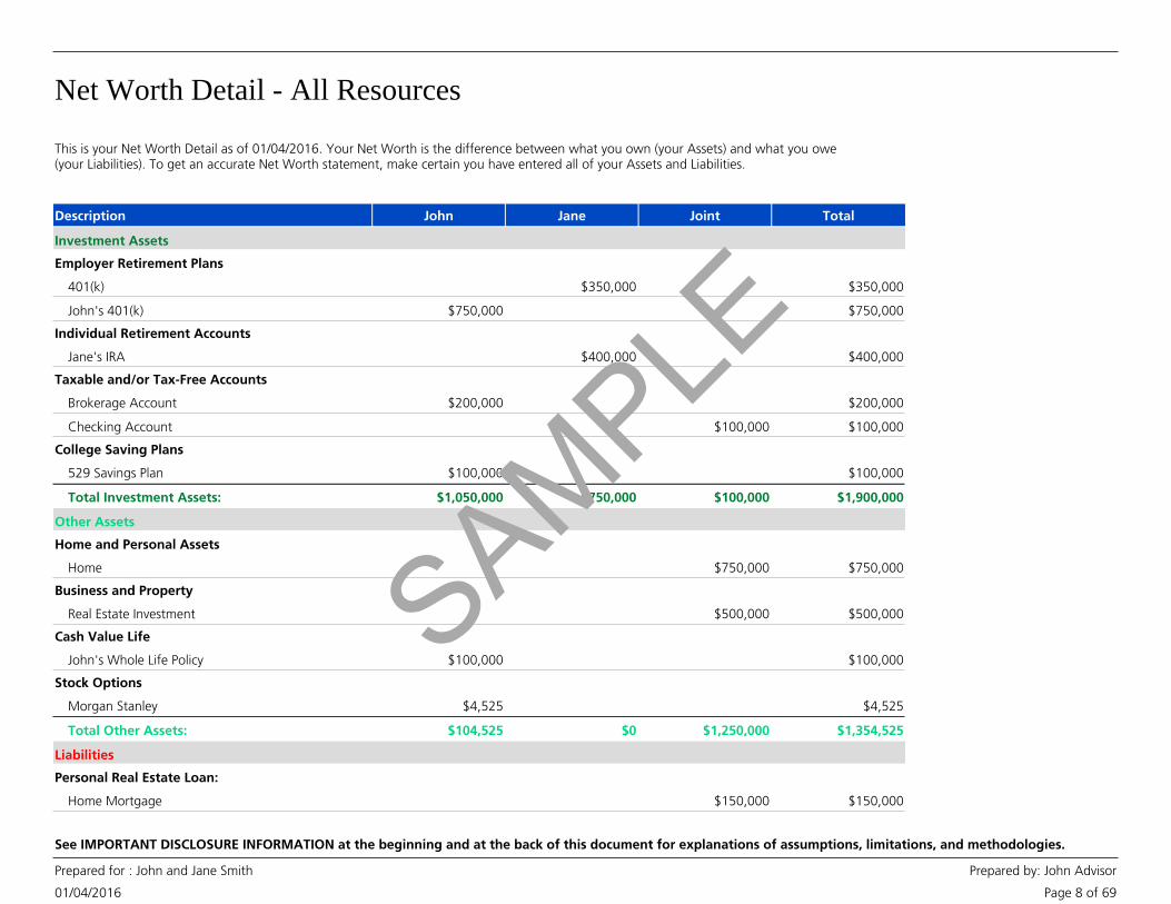
This is your Net Worth Detail as of 01/04/2016. Your Net Worth is the difference between what you own (your Assets) and what you owe(your Liabilities). To get an accurate Net Worth statement, make certain you have entered all of your Assets and Liabilities.
Description TotalJointJaneJohn
Investment Assets
Employer Retirement Plans
401(k) $350,000$350,000
John's 401(k) $750,000$750,000
Individual Retirement Accounts
Jane's IRA $400,000$400,000
Taxable and/or Tax-Free Accounts
Brokerage Account $200,000$200,000
Checking Account $100,000$100,000
College Saving Plans
529 Savings Plan $100,000$100,000
Total Investment Assets: $1,900,000$1,050,000 $750,000 $100,000
Other Assets
Home and Personal Assets
Home $750,000$750,000
Business and Property
Real Estate Investment $500,000$500,000
Cash Value Life
John's Whole Life Policy $100,000$100,000
Stock Options
Morgan Stanley $4,525$4,525
Total Other Assets: $1,354,525$104,525 $0 $1,250,000
Liabilities
Personal Real Estate Loan:
Home Mortgage $150,000$150,000
SAMPLE
Net Worth Detail - All Resources
01/04/2016
Prepared for : John and Jane Smith Prepared by: John Advisor
Page 9 of 69
See IMPORTANT DISCLOSURE INFORMATION at the beginning and at the back of this document for explanations of assumptions, limitations, and methodologies.
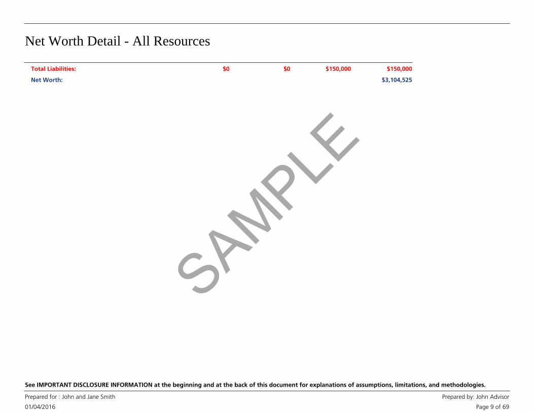
Total Liabilities: $150,000$0 $0 $150,000
Net Worth: $3,104,525
SAMPLE
Resources Summary
01/04/2016
Prepared for : John and Jane Smith Prepared by: John Advisor
Page 10 of 69
See IMPORTANT DISCLOSURE INFORMATION at the beginning and at the back of this document for explanations of assumptions, limitations, and methodologies.
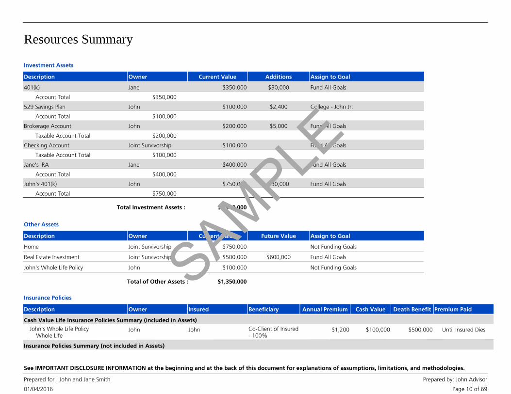
Description Owner Current Value Additions Assign to Goal
Investment Assets
Jane401(k) $350,000 $30,000 Fund All Goals
$350,000Account Total
John529 Savings Plan $100,000 $2,400 College - John Jr.
$100,000Account Total
JohnBrokerage Account $200,000 $5,000 Fund All Goals
$200,000Taxable Account Total
Joint SurvivorshipChecking Account $100,000 Fund All Goals
$100,000Taxable Account Total
JaneJane's IRA $400,000 Fund All Goals
$400,000Account Total
JohnJohn's 401(k) $750,000 $30,000 Fund All Goals
$750,000Account Total
$1,900,000Total Investment Assets :
Description Owner Current Value Future Value Assign to Goal
Other Assets
Home Joint Survivorship $750,000 Not Funding Goals
Real Estate Investment Joint Survivorship $500,000 $600,000 Fund All Goals
John's Whole Life Policy John $100,000 Not Funding Goals
$1,350,000Total of Other Assets :
Annual Premium Cash ValueDescription Owner BeneficiaryInsured Death Benefit Premium Paid
Insurance Policies
Cash Value Life Insurance Policies Summary (included in Assets)
$1,200 $100,000John's Whole Life Policy Whole Life
John Co-Client of Insured- 100%
John $500,000 Until Insured Dies
Insurance Policies Summary (not included in Assets)
SAMPLE
Resources Summary
01/04/2016
Prepared for : John and Jane Smith Prepared by: John Advisor
Page 11 of 69
See IMPORTANT DISCLOSURE INFORMATION at the beginning and at the back of this document for explanations of assumptions, limitations, and methodologies.
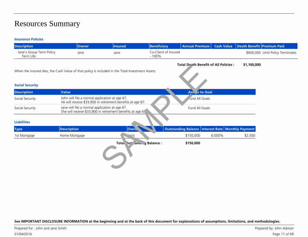
Annual Premium Cash ValueDescription Owner BeneficiaryInsured Death Benefit Premium Paid
Insurance Policies
Jane's Group Term Policy Term Life
Jane Co-Client of Insured- 100%
Jane $600,000 Until Policy Terminates
$1,100,000Total Death Benefit of All Policies :
When the insured dies, the Cash Value of that policy is included in the Total Investment Assets.
Social Security
Description Value Assign to Goal
Social Security John will file a normal application at age 67.He will receive $33,900 in retirement benefits at age 67.
Fund All Goals
Social Security Jane will file a normal application at age 67.She will receive $33,900 in retirement benefits at age 67.
Fund All Goals
Type Outstanding Balance Monthly PaymentDescription Interest RateOwner
Liabilities
1st Mortgage Home Mortgage $150,000 $2,5006.000%Joint
$150,000Total Outstanding Balance :
SAMPLE
Current Portfolio Allocation
01/04/2016
Prepared for : John and Jane Smith Prepared by: John Advisor
Page 12 of 69
See IMPORTANT DISCLOSURE INFORMATION at the beginning and at the back of this document for explanations of assumptions, limitations, and methodologies.
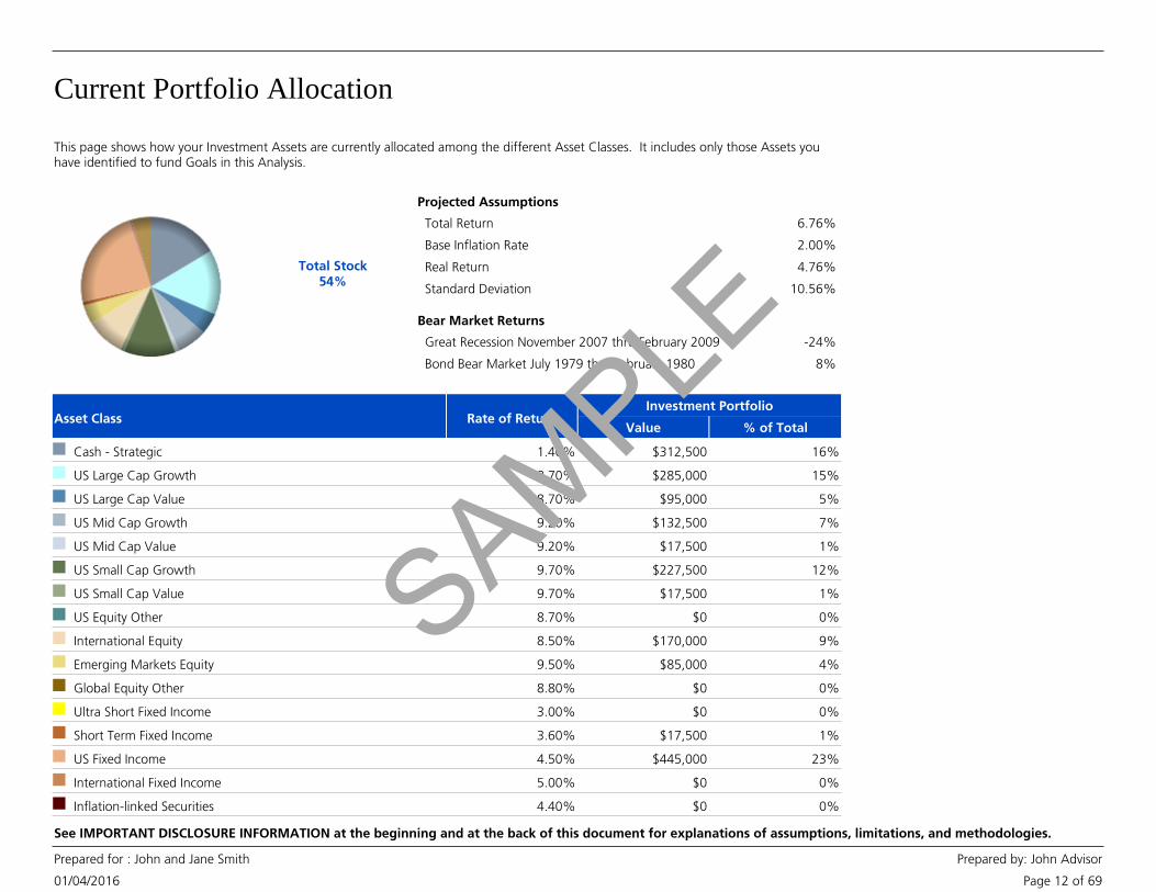
Total Stock54%
This page shows how your Investment Assets are currently allocated among the different Asset Classes. It includes only those Assets youhave identified to fund Goals in this Analysis.
Projected Assumptions
Total Return 6.76%
Base Inflation Rate 2.00%
Real Return 4.76%
Standard Deviation 10.56%
Bear Market Returns
Great Recession November 2007 thru February 2009 -24%
Bond Bear Market July 1979 thru February 1980 8%
Asset Class Rate of ReturnValue % of Total
Investment Portfolio
16%$312,5001.40%Cash - Strategic
15%$285,0008.70%US Large Cap Growth
5%$95,0008.70%US Large Cap Value
7%$132,5009.20%US Mid Cap Growth
1%$17,5009.20%US Mid Cap Value
12%$227,5009.70%US Small Cap Growth
1%$17,5009.70%US Small Cap Value
0%$08.70%US Equity Other
9%$170,0008.50%International Equity
4%$85,0009.50%Emerging Markets Equity
0%$08.80%Global Equity Other
0%$03.00%Ultra Short Fixed Income
1%$17,5003.60%Short Term Fixed Income
23%$445,0004.50%US Fixed Income
0%$05.00%International Fixed Income
0%$04.40%Inflation-linked Securities
SAMPLE
Current Portfolio Allocation
01/04/2016
Prepared for : John and Jane Smith Prepared by: John Advisor
Page 13 of 69
See IMPORTANT DISCLOSURE INFORMATION at the beginning and at the back of this document for explanations of assumptions, limitations, and methodologies.
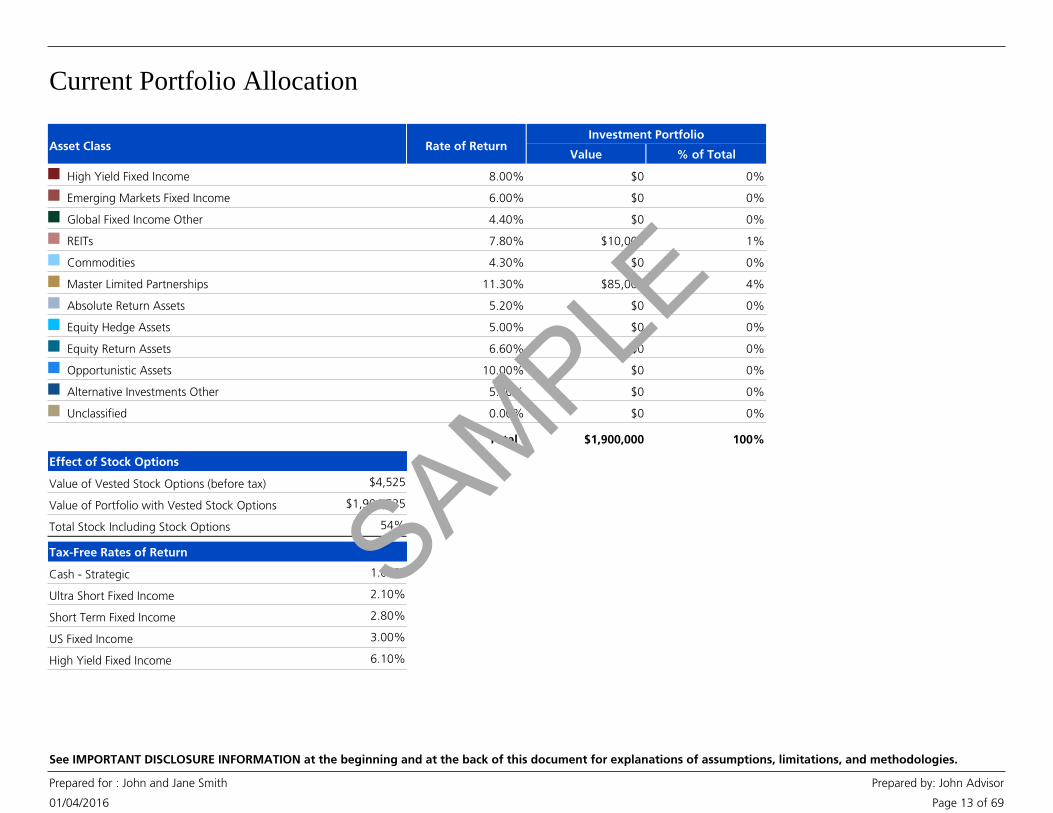
Asset Class Rate of ReturnValue % of Total
Investment Portfolio
0%$08.00%High Yield Fixed Income
0%$06.00%Emerging Markets Fixed Income
0%$04.40%Global Fixed Income Other
1%$10,0007.80%REITs
0%$04.30%Commodities
4%$85,00011.30%Master Limited Partnerships
0%$05.20%Absolute Return Assets
0%$05.00%Equity Hedge Assets
0%$06.60%Equity Return Assets
0%$010.00%Opportunistic Assets
0%$05.80%Alternative Investments Other
0%$00.00%Unclassified
Total : 100%$1,900,000
Effect of Stock Options
Value of Vested Stock Options (before tax) $4,525
Value of Portfolio with Vested Stock Options $1,904,525
Total Stock Including Stock Options 54%
Tax-Free Rates of Return
1.00%Cash - Strategic
2.10%Ultra Short Fixed Income
2.80%Short Term Fixed Income
3.00%US Fixed Income
6.10%High Yield Fixed Income
SAMPLE
Target Band
01/04/2016
Prepared for : John and Jane Smith Prepared by: John Advisor
Page 14 of 69
See IMPORTANT DISCLOSURE INFORMATION at the beginning and at the back of this document for explanations of assumptions, limitations, and methodologies.
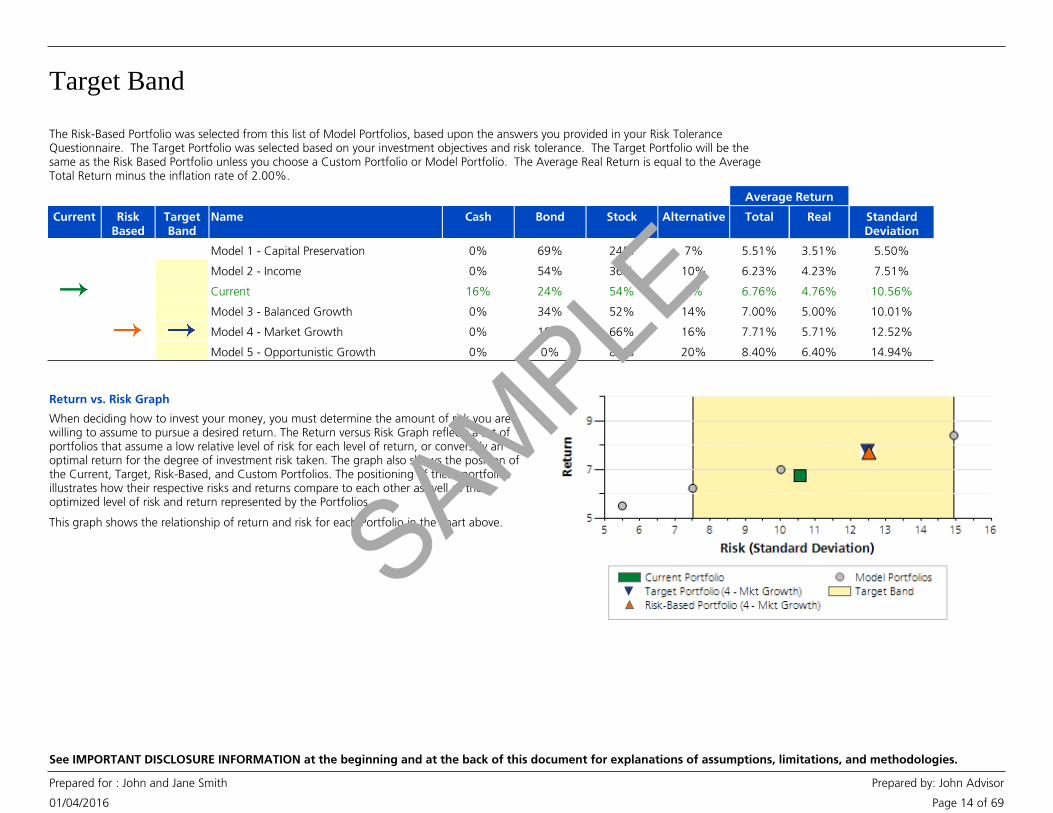
The Risk-Based Portfolio was selected from this list of Model Portfolios, based upon the answers you provided in your Risk ToleranceQuestionnaire. The Target Portfolio was selected based on your investment objectives and risk tolerance. The Target Portfolio will be thesame as the Risk Based Portfolio unless you choose a Custom Portfolio or Model Portfolio. The Average Real Return is equal to the AverageTotal Return minus the inflation rate of 2.00%.
RiskBased
TargetBand
Name TotalStock RealCurrent
Average Return
StandardDeviation
BondCash Alternative
Model 1 - Capital Preservation 5.51%24% 3.51% 5.50%69%0% 7%
Model 2 - Income 6.23%36% 4.23% 7.51%54%0% 10%
Current 6.76%54% 4.76% 10.56%24%16% 5%
Model 3 - Balanced Growth 7.00%52% 5.00% 10.01%34%0% 14%
Model 4 - Market Growth 7.71%66% 5.71% 12.52%18%0% 16%
Model 5 - Opportunistic Growth 8.40%80% 6.40% 14.94%0%0% 20%
Return vs. Risk Graph
This graph shows the relationship of return and risk for each Portfolio in the chart above.
When deciding how to invest your money, you must determine the amount of risk you arewilling to assume to pursue a desired return. The Return versus Risk Graph reflects a set ofportfolios that assume a low relative level of risk for each level of return, or conversely anoptimal return for the degree of investment risk taken. The graph also shows the position ofthe Current, Target, Risk-Based, and Custom Portfolios. The positioning of these portfoliosillustrates how their respective risks and returns compare to each other as well as theoptimized level of risk and return represented by the Portfolios.
SAMPLE

Results
SAMPLE
What If Worksheet
01/04/2016
Prepared for : John and Jane Smith Prepared by: John Advisor
Page 15 of 69
See IMPORTANT DISCLOSURE INFORMATION at the beginning and at the back of this document for explanations of assumptions, limitations, and methodologies.
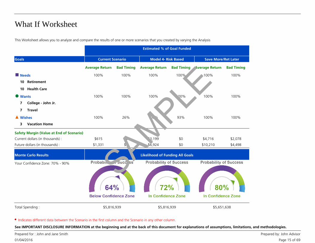
This Worksheet allows you to analyze and compare the results of one or more scenarios that you created by varying the Analysisassumptions.
Goals
Estimated % of Goal Funded
Current Scenario Model 4- Risk Based Save More/Ret Later
Average Return Bad Timing Average Return Bad Timing Average Return Bad Timing
Needs 100% 100% 100% 100% 100% 100%
10 Retirement
10 Health Care
Wants 100% 100% 100% 100% 100% 100%
7 College - John Jr.
7 Travel
Wishes 100% 26% 100% 93% 100% 100%
3 Vacation Home
$615
$1,331
Current dollars (in thousands) :
Future dollars (in thousands) :
$3,199
$6,924
Safety Margin (Value at End of Scenario)
$4,716
$10,210
$0
$0
$0
$0
$2,078
$4,498
Your Confidence Zone: 70% - 90%
Likelihood of Funding All GoalsMonte Carlo Results
Total Spending : $5,816,939 $5,816,939 $5,651,638
Indicates different data between the Scenario in the first column and the Scenario in any other column.
SAMPLE
What If Worksheet
01/04/2016
Prepared for : John and Jane Smith Prepared by: John Advisor
Page 16 of 69
See IMPORTANT DISCLOSURE INFORMATION at the beginning and at the back of this document for explanations of assumptions, limitations, and methodologies.
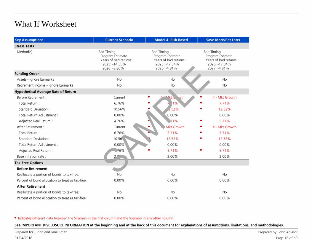
Key Assumptions Current Scenario Model 4- Risk Based Save More/Ret Later
Stress Tests
Method(s) Bad Timing Program Estimate Years of bad returns: 2025: -14.35% 2026: -3.80%
Bad Timing Program Estimate Years of bad returns: 2025: -17.34% 2026: -4.81%
Bad Timing Program Estimate Years of bad returns: 2026: -17.34% 2027: -4.81%
False 0
Funding Order
Assets - Ignore Earmarks No No No False 1
Retirement Income - Ignore Earmarks No No No False 1
Hypothetical Average Rate of Return
Before Retirement : Current 4 - Mkt Growth 4 - Mkt Growth False 1
Total Return : 6.76% 7.71% 7.71% False 1
Standard Deviation : 10.56% 12.52% 12.52% False 1
Total Return Adjustment : 0.00% 0.00% 0.00% False 1
Adjusted Real Return : 4.76% 5.71% 5.71% False 1
After Retirement : Current 4 - Mkt Growth 4 - Mkt Growth False 1
Total Return : 6.76% 7.71% 7.71% False 1
Standard Deviation : 10.56% 12.52% 12.52% False 1
Total Return Adjustment : 0.00% 0.00% 0.00% False 1
Adjusted Real Return : 4.76% 5.71% 5.71% False 1
Base inflation rate : 2.00% 2.00% 2.00% False 1
Tax-Free Options
Before Retirement True 1
Reallocate a portion of bonds to tax-free: No No No False 1
Percent of bond allocation to treat as tax-free: 0.00% 0.00% 0.00% False 1
After Retirement True 1
Reallocate a portion of bonds to tax-free: No No No False 1
Percent of bond allocation to treat as tax-free: 0.00% 0.00% 0.00% False 1
Indicates different data between the Scenario in the first column and the Scenario in any other column.
SAMPLE
What If Worksheet
01/04/2016
Prepared for : John and Jane Smith Prepared by: John Advisor
Page 17 of 69
See IMPORTANT DISCLOSURE INFORMATION at the beginning and at the back of this document for explanations of assumptions, limitations, and methodologies.
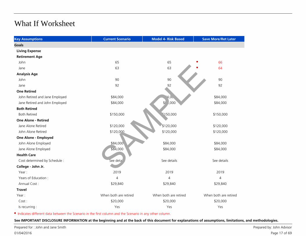
Key Assumptions Current Scenario Model 4- Risk Based Save More/Ret Later
Goals
Living Expense True 1
Retirement Age True 1
John 65 65 66 False 1
Jane 63 63 64 False 1
Analysis Age True 1
John 90 90 90 False 1
Jane 92 92 92 False 1
One Retired True 1
John Retired and Jane Employed $84,000 $84,000 $84,000 False 1
Jane Retired and John Employed $84,000 $84,000 $84,000 False 1
Both Retired True 1
Both Retired $150,000 $150,000 $150,000 False 1
One Alone - Retired True 1
Jane Alone Retired $120,000 $120,000 $120,000 False 1
John Alone Retired $120,000 $120,000 $120,000 False 1
One Alone - Employed True 1
John Alone Employed $84,000 $84,000 $84,000 False 1
Jane Alone Employed $84,000 $84,000 $84,000 False 1
Health Care True 1
Cost determined by Schedule : See details See details See details False 1
College - John Jr. True 1
Year : 2019 2019 2019 False 1
Years of Education : 4 4 4 False 1
Annual Cost : $29,840 $29,840 $29,840 False 1
Travel True 1
Year : When both are retired When both are retired When both are retired False 1
Cost : $20,000 $20,000 $20,000 False 1
Is recurring : Yes Yes Yes False 1
Indicates different data between the Scenario in the first column and the Scenario in any other column.
SAMPLE
What If Worksheet
01/04/2016
Prepared for : John and Jane Smith Prepared by: John Advisor
Page 18 of 69
See IMPORTANT DISCLOSURE INFORMATION at the beginning and at the back of this document for explanations of assumptions, limitations, and methodologies.
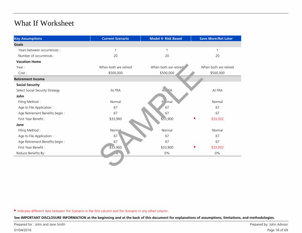
Key Assumptions Current Scenario Model 4- Risk Based Save More/Ret Later
Goals
Years between occurrences : 1 1 1 False 1
Number of occurrences : 20 20 20 False 1
Vacation Home True 1
Year : When both are retired When both are retired When both are retired False 1
Cost : $500,000 $500,000 $500,000 False 1
Retirement Income
Social Security True 1
Select Social Security Strategy At FRA At FRA At FRA False 1
John True 1
Filing Method : Normal Normal Normal False 1
Age to File Application : 67 67 67 False 1
Age Retirement Benefits begin : 67 67 67 False 1
First Year Benefit : $33,900 $33,900 $33,932 False 1
Jane True 1
Filing Method : Normal Normal Normal False 1
Age to File Application : 67 67 67 False 1
Age Retirement Benefits begin : 67 67 67 False 1
First Year Benefit : $33,900 $33,900 $33,932 False 1
Reduce Benefits By : 0% 0% 0% False 1
Indicates different data between the Scenario in the first column and the Scenario in any other column.
SAMPLE
What If Worksheet
01/04/2016
Prepared for : John and Jane Smith Prepared by: John Advisor
Page 19 of 69
See IMPORTANT DISCLOSURE INFORMATION at the beginning and at the back of this document for explanations of assumptions, limitations, and methodologies.
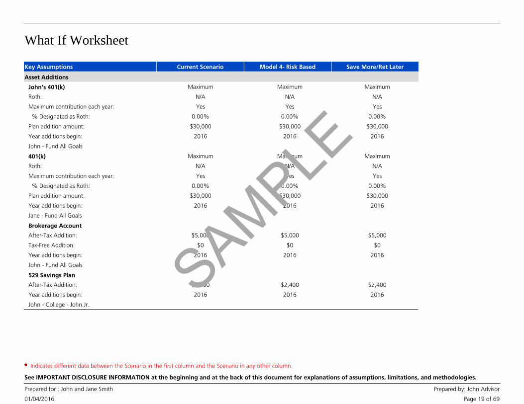
Key Assumptions Current Scenario Model 4- Risk Based Save More/Ret Later
Asset Additions
John's 401(k) Maximum Maximum Maximum True 1
Roth: N/A N/A N/A False 1
Maximum contribution each year: Yes Yes Yes False 1
% Designated as Roth: 0.00% 0.00% 0.00% False 1
Plan addition amount: $30,000 $30,000 $30,000 False 1
Year additions begin: 2016 2016 2016 False 1
John - Fund All Goals False 1
401(k) Maximum Maximum Maximum True 1
Roth: N/A N/A N/A False 1
Maximum contribution each year: Yes Yes Yes False 1
% Designated as Roth: 0.00% 0.00% 0.00% False 1
Plan addition amount: $30,000 $30,000 $30,000 False 1
Year additions begin: 2016 2016 2016 False 1
Jane - Fund All Goals False 1
Brokerage Account True 1
After-Tax Addition: $5,000 $5,000 $5,000 False 1
Tax-Free Addition: $0 $0 $0 False 1
Year additions begin: 2016 2016 2016 False 1
John - Fund All Goals False 1
529 Savings Plan True 1
After-Tax Addition: $2,400 $2,400 $2,400 False 1
Year additions begin: 2016 2016 2016 False 1
John - College - John Jr. False 1
Indicates different data between the Scenario in the first column and the Scenario in any other column.
SAMPLE
What If Worksheet
01/04/2016
Prepared for : John and Jane Smith Prepared by: John Advisor
Page 20 of 69
See IMPORTANT DISCLOSURE INFORMATION at the beginning and at the back of this document for explanations of assumptions, limitations, and methodologies.
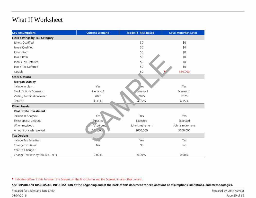
Key Assumptions Current Scenario Model 4- Risk Based Save More/Ret Later
Extra Savings by Tax Category
John's Qualified $0 $0 False 1
Jane's Qualified $0 $0 False 1
John's Roth $0 $0 False 1
Jane's Roth $0 $0 False 1
John's Tax-Deferred $0 $0 False 1
Jane's Tax-Deferred $0 $0 False 1
Taxable $0 $10,000 False 1
Stock Options
Morgan Stanley True 1
Include in plan : Yes Yes Yes False 1
Stock Options Scenario : Scenario 1 Scenario 1 Scenario 1 False 1
Vesting Termination Year : 2025 2025 2025 False 1
Return : 4.35% 4.35% 4.35% False 1
Other Assets
Real Estate Investment True 1
Include in Analysis : Yes Yes Yes False 1
Select special amount : Expected Expected Expected False 1
When received : John's retirement John's retirement John's retirement False 1
Amount of cash received : $600,000 $600,000 $600,000 False 1
Tax Options
Include Tax Penalties : Yes Yes Yes False 1
Change Tax Rate? No No No False 1
Year To Change : False 1
Change Tax Rate by this % (+ or -) : 0.00% 0.00% 0.00% False 1
Indicates different data between the Scenario in the first column and the Scenario in any other column.
SAMPLE
Worksheet Detail - Combined Details
01/04/2016
Prepared for : John and Jane Smith Prepared by: John Advisor
Page 21 of 69
See IMPORTANT DISCLOSURE INFORMATION at the beginning and at the back of this document for explanations of assumptions, limitations, and methodologies.
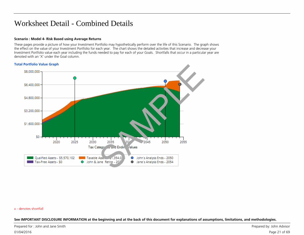
Total Portfolio Value Graph
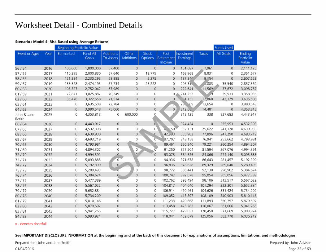
These pages provide a picture of how your Investment Portfolio may hypothetically perform over the life of this Scenario. The graph showsthe effect on the value of your Investment Portfolio for each year. The chart shows the detailed activities that increase and decrease yourInvestment Portfolio value each year including the funds needed to pay for each of your Goals. Shortfalls that occur in a particular year aredenoted with an 'X' under the Goal column.
Scenario : Model 4- Risk Based using Average Returns
x - denotes shortfall
SAMPLE
Worksheet Detail - Combined Details
01/04/2016
Prepared for : John and Jane Smith Prepared by: John Advisor
Page 22 of 69
See IMPORTANT DISCLOSURE INFORMATION at the beginning and at the back of this document for explanations of assumptions, limitations, and methodologies.
Event or Ages Year
Beginning Portfolio Value
Earmarked Fund AllGoals
AdditionsTo Assets
OtherAdditions
StockOptions
PostRetirement
Income
InvestmentEarnings
Taxes
Funds Used
All Goals EndingPortfolio
Value
56 / 54 2016 100,000 1,800,000 67,400 0 0 0 151,687 7,961 0 2,111,125
57 / 55 2017 110,295 2,000,830 67,640 0 12,775 0 168,968 8,831 0 2,351,677
58 / 56 2018 121,384 2,230,293 68,885 0 9,275 0 187,340 9,654 0 2,607,523
59 / 57 2019 133,328 2,474,195 67,734 0 23,222 0 205,313 10,883 35,540 2,857,369
60 / 58 2020 105,327 2,752,042 67,989 0 0 0 222,641 11,569 37,672 3,098,757
61 / 59 2021 72,871 3,025,887 70,249 0 0 0 241,252 12,289 39,933 3,358,036
62 / 60 2022 35,478 3,322,558 71,514 0 0 0 261,155 12,868 42,329 3,635,508
63 / 61 2023 0 3,635,508 72,784 0 0 0 285,909 13,654 0 3,980,548
64 / 62 2024 0 3,980,548 75,060 0 0 0 312,687 14,481 0 4,353,813
John & JaneRetire
2025 0 4,353,813 0 600,000 0 0 318,125 338 827,683 4,443,917
66 / 64 2026 0 4,443,917 0 0 0 0 324,434 0 235,953 4,532,398
67 / 65 2027 0 4,532,398 0 0 0 42,150 332,131 25,622 241,128 4,639,930
68 / 66 2028 0 4,639,930 0 0 0 42,993 335,982 77,896 247,290 4,693,719
69 / 67 2029 0 4,693,719 0 0 0 87,707 343,158 76,941 253,662 4,793,981
70 / 68 2030 0 4,793,981 0 0 0 89,461 350,340 79,221 260,254 4,894,307
71 / 69 2031 0 4,894,307 0 0 0 91,250 357,504 81,594 267,076 4,994,391
72 / 70 2032 0 4,994,391 0 0 0 93,075 364,626 84,066 274,140 5,093,885
73 / 71 2033 0 5,093,885 0 0 0 94,936 371,678 86,643 281,457 5,192,399
74 / 72 2034 0 5,192,399 0 0 0 96,835 378,628 89,329 289,040 5,289,493
75 / 73 2035 0 5,289,493 0 0 0 98,772 385,441 92,130 296,902 5,384,674
76 / 74 2036 0 5,384,674 0 0 0 100,747 392,078 95,054 305,056 5,477,389
77 / 75 2037 0 5,477,389 0 0 0 102,762 398,494 98,106 313,517 5,567,022
78 / 76 2038 0 5,567,022 0 0 0 104,817 404,640 101,294 322,301 5,652,884
79 / 77 2039 0 5,652,884 0 0 0 106,914 410,461 104,626 331,424 5,734,209
80 / 78 2040 0 5,734,209 0 0 0 109,052 415,897 108,109 340,903 5,810,146
81 / 79 2041 0 5,810,146 0 0 0 111,233 420,868 111,893 350,757 5,879,597
82 / 80 2042 0 5,879,597 0 0 0 113,458 425,282 116,067 361,006 5,941,265
83 / 81 2043 0 5,941,265 0 0 0 115,727 429,052 120,450 371,669 5,993,924
84 / 82 2044 0 5,993,924 0 0 0 118,041 432,079 125,056 382,770 6,036,219
Scenario : Model 4- Risk Based using Average Returns
x - denotes shortfall
SAMPLE
Worksheet Detail - Combined Details
01/04/2016
Prepared for : John and Jane Smith Prepared by: John Advisor
Page 23 of 69
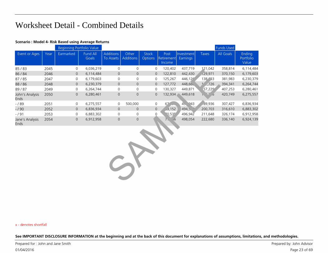
See IMPORTANT DISCLOSURE INFORMATION at the beginning and at the back of this document for explanations of assumptions, limitations, and methodologies.
Event or Ages Year
Beginning Portfolio Value
Earmarked Fund AllGoals
AdditionsTo Assets
OtherAdditions
StockOptions
PostRetirement
Income
InvestmentEarnings
Taxes
Funds Used
All Goals EndingPortfolio
Value
85 / 83 2045 0 6,036,219 0 0 0 120,402 437,719 121,042 358,814 6,114,484
86 / 84 2046 0 6,114,484 0 0 0 122,810 442,430 129,971 370,150 6,179,603
87 / 85 2047 0 6,179,603 0 0 0 125,267 446,126 138,633 381,983 6,230,379
88 / 86 2048 0 6,230,379 0 0 0 127,772 448,660 147,726 394,341 6,264,744
89 / 87 2049 0 6,264,744 0 0 0 130,327 449,871 157,229 407,253 6,280,461
John's AnalysisEnds
2050 0 6,280,461 0 0 0 132,934 449,618 166,706 420,749 6,275,557
- / 89 2051 0 6,275,557 0 500,000 0 67,796 490,943 189,936 307,427 6,836,934
- / 90 2052 0 6,836,934 0 0 0 69,152 494,530 200,703 316,610 6,883,302
- / 91 2053 0 6,883,302 0 0 0 70,535 496,942 211,648 326,174 6,912,958
Jane's AnalysisEnds
2054 0 6,912,958 0 0 0 71,946 498,054 222,680 336,140 6,924,139
Scenario : Model 4- Risk Based using Average Returns
x - denotes shortfall
SAMPLE
Worksheet Detail - Combined Details
01/04/2016
Prepared for : John and Jane Smith Prepared by: John Advisor
Page 24 of 69
See IMPORTANT DISCLOSURE INFORMATION at the beginning and at the back of this document for explanations of assumptions, limitations, and methodologies.
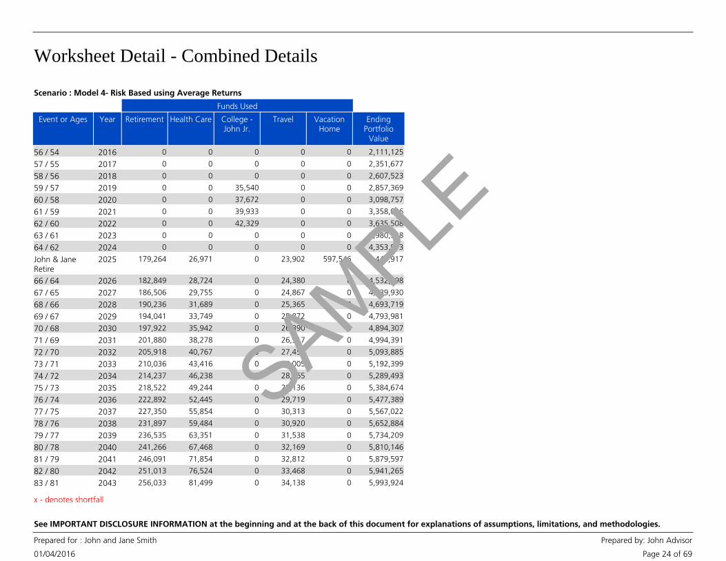
Scenario : Model 4- Risk Based using Average Returns
Event or Ages Year
Funds Used
Retirement Health Care College -John Jr.
Travel VacationHome
EndingPortfolio
Value
56 / 54 2016 0 0 0 0 0 2,111,125
57 / 55 2017 0 0 0 0 0 2,351,677
58 / 56 2018 0 0 0 0 0 2,607,523
59 / 57 2019 0 0 35,540 0 0 2,857,369
60 / 58 2020 0 0 37,672 0 0 3,098,757
61 / 59 2021 0 0 39,933 0 0 3,358,036
62 / 60 2022 0 0 42,329 0 0 3,635,508
63 / 61 2023 0 0 0 0 0 3,980,548
64 / 62 2024 0 0 0 0 0 4,353,813
John & JaneRetire
2025 179,264 26,971 0 23,902 597,546 4,443,917
66 / 64 2026 182,849 28,724 0 24,380 0 4,532,398
67 / 65 2027 186,506 29,755 0 24,867 0 4,639,930
68 / 66 2028 190,236 31,689 0 25,365 0 4,693,719
69 / 67 2029 194,041 33,749 0 25,872 0 4,793,981
70 / 68 2030 197,922 35,942 0 26,390 0 4,894,307
71 / 69 2031 201,880 38,278 0 26,917 0 4,994,391
72 / 70 2032 205,918 40,767 0 27,456 0 5,093,885
73 / 71 2033 210,036 43,416 0 28,005 0 5,192,399
74 / 72 2034 214,237 46,238 0 28,565 0 5,289,493
75 / 73 2035 218,522 49,244 0 29,136 0 5,384,674
76 / 74 2036 222,892 52,445 0 29,719 0 5,477,389
77 / 75 2037 227,350 55,854 0 30,313 0 5,567,022
78 / 76 2038 231,897 59,484 0 30,920 0 5,652,884
79 / 77 2039 236,535 63,351 0 31,538 0 5,734,209
80 / 78 2040 241,266 67,468 0 32,169 0 5,810,146
81 / 79 2041 246,091 71,854 0 32,812 0 5,879,597
82 / 80 2042 251,013 76,524 0 33,468 0 5,941,265
83 / 81 2043 256,033 81,499 0 34,138 0 5,993,924
x - denotes shortfall
SAMPLE
Worksheet Detail - Combined Details
01/04/2016
Prepared for : John and Jane Smith Prepared by: John Advisor
Page 25 of 69
See IMPORTANT DISCLOSURE INFORMATION at the beginning and at the back of this document for explanations of assumptions, limitations, and methodologies.
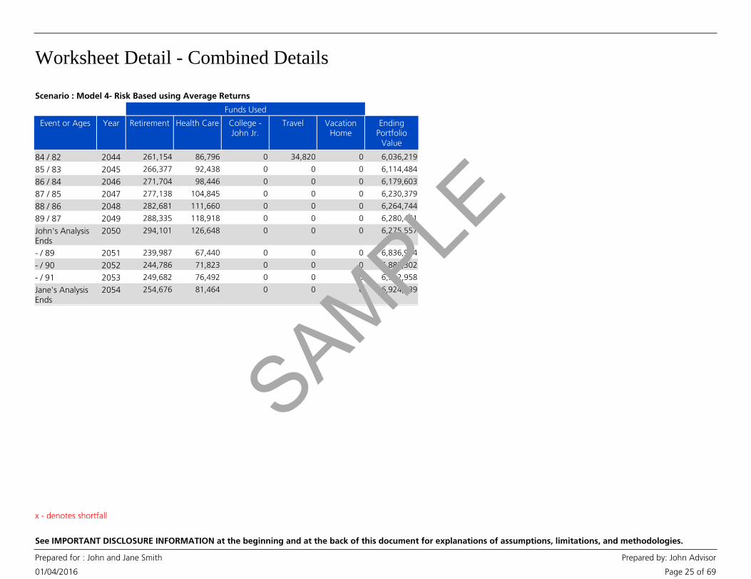
Scenario : Model 4- Risk Based using Average Returns
Event or Ages Year
Funds Used
Retirement Health Care College -John Jr.
Travel VacationHome
EndingPortfolio
Value
84 / 82 2044 261,154 86,796 0 34,820 0 6,036,219
85 / 83 2045 266,377 92,438 0 0 0 6,114,484
86 / 84 2046 271,704 98,446 0 0 0 6,179,603
87 / 85 2047 277,138 104,845 0 0 0 6,230,379
88 / 86 2048 282,681 111,660 0 0 0 6,264,744
89 / 87 2049 288,335 118,918 0 0 0 6,280,461
John's AnalysisEnds
2050 294,101 126,648 0 0 0 6,275,557
- / 89 2051 239,987 67,440 0 0 0 6,836,934
- / 90 2052 244,786 71,823 0 0 0 6,883,302
- / 91 2053 249,682 76,492 0 0 0 6,912,958
Jane's AnalysisEnds
2054 254,676 81,464 0 0 0 6,924,139
x - denotes shortfall
SAMPLE

Worksheet Detail - Combined Details
01/04/2016
Prepared for : John and Jane Smith Prepared by: John Advisor
Page 26 of 69
See IMPORTANT DISCLOSURE INFORMATION at the beginning and at the back of this document for explanations of assumptions, limitations, and methodologies.
Notes
• IMPORTANT: The projections or other information generated by this tool regarding thelikelihood of various investment outcomes are hypothetical in nature, do not reflect actualinvestment results, and are not guarantees of future results.
• Results may vary with use and over time.
• The return assumptions used are estimates based on average annual returns for the indexused as a proxy for each asset class. The portfolio returns were calculated by weightingindividual return assumptions for each asset class according to the portfolio allocationselected by you or your Financial Advisor. The portfolio returns may have also been modifiedby your Financial Advisor to reflect the outcome of a different return by conducting a TotalReturn Adjustment or selecting a Custom Portfolio. For a explanation of the methodologyused to calculate returns, please review the Important Disclosure Information and ReturnMethodology sections.
• The return assumptions in this tool are not reflective of any specific product and do notinclude any fees or expenses that may be incurred by investing in specific products. Theactual returns of a specific product may be more or less than the returns used in this tool.
• No investment strategy or allocation can eliminate risk or guarantee investment results.
• Additions and withdrawals occur at the beginning of the year.
• Other Additions come from items entered in the Other Assets section and any applicableproceeds from insurance policies.
• Stock Options and Restricted Stock values are after-tax and based on the Exercise Scenarioselected.
• Strategy Income is based on the particulars of the Goal Strategies selected. StrategyIncome from immediate annuities and 72(t) distributions is pre-tax. Strategy Income fromNet Unrealized Appreciation (NUA) is after-tax.
• Post Retirement Income includes the following: Social Security, pension, annuity, rentalproperty, royalty, alimony, part-time employment, trust, and any other retirement income asentered in the Scenario.
• For married clients, if either Social Security Program Estimate or Use This Amount andEvaluate Annually is selected for a participant, the Program defaults to the greater of theselected benefit or the age-adjusted spousal benefit based on the other participant’sbenefit. The spousal benefit is not applicable to domestic partners.
• Investment Earnings are calculated on all assets after any withdrawals for 'Goal Expense','Taxes on Withdrawals' and 'Tax Penalties' are subtracted.
• The taxes column is a sum of (1) taxes on retirement income, (2) taxes on strategy income,(3) taxes on withdrawals from qualified assets for Required Minimum Distributions, (4) taxeson withdrawals from taxable assets' untaxed gain used to fund Goals in that year, (5) taxeson withdrawals from tax-deferred or qualified assets used to fund Goals in that year, and (6)taxes on the investment earnings of taxable assets. Tax rates used are detailed in the Taxand Inflation Options page. (Please note, the Taxes column does not include any taxesowed from the exercise of Stock Options or the vesting of Restricted Stock.)
• Tax Penalties can occur when Qualified and Tax-Deferred Assets are used prior to age59½. If there is a value in this column, it illustrates that you are using your assets in thisScenario in a manner that may incur tax penalties. Generally, it is better to avoid taxpenalties whenever possible.
• These calculations do not incorporate penalties associated with use of 529 Planwithdrawals for non-qualified expenses.
• Funds for each Goal Expense are used first from Earmarked Assets. If sufficient funds arenot available from Earmarked Assets, Fund All Goals Assets will be used to fund theremaining portion of the Goal Expense, if available in that year.
• All funds needed for a Goal must be available in the year the Goal occurs. Funds fromEarmarked Assets that become available after the Goal year(s) have passed are not includedin the funding of that Goal, and accumulate until the end of the Scenario.
• For married clients, ownership of qualified assets is assumed to roll over to the survivingco-client at the death of the original owner. For domestic partners, qualified assets areassumed to be transferred as a non-spousal inheritance to the surviving co-client at thedeath of the original owner. In both cases, the Program assumes the surviving co-clientinherits all remaining assets of the original owner.
x - denotes shortfall
SAMPLE
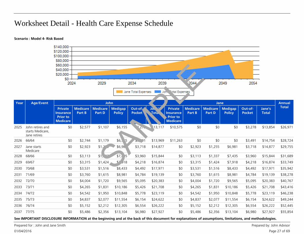
Worksheet Detail - Health Care Expense Schedule
01/04/2016
Prepared for : John and Jane Smith Prepared by: John Advisor
Page 27 of 69
See IMPORTANT DISCLOSURE INFORMATION at the beginning and at the back of this document for explanations of assumptions, limitations, and methodologies.
Year Age/Event John
PrivateInsurancePrior to
Medicare
MedicarePart B
MedicarePart D
MedigapPolicy
Out-of-Pocket
John'sTotal
Jane
PrivateInsurancePrior to
Medicare
MedicarePart B
MedicarePart D
MedigapPolicy
Out-of-Pocket
Jane'sTotal
AnnualTotal
2025 John retires andstarts Medicare,Jane retires
$0 $2,577 $1,107 $6,155 $3,278 $13,117 $10,575 $0 $0 $0 $3,278 $13,854 $26,971
2026 66/64 $0 $2,744 $1,179 $6,555 $3,491 $13,969 $11,263 $0 $0 $0 $3,491 $14,754 $28,724
2027 Jane startsMedicare
$0 $2,923 $1,255 $6,981 $3,718 $14,877 $0 $2,923 $1,255 $6,981 $3,718 $14,877 $29,755
2028 68/66 $0 $3,113 $1,337 $7,435 $3,960 $15,844 $0 $3,113 $1,337 $7,435 $3,960 $15,844 $31,689
2029 69/67 $0 $3,315 $1,424 $7,918 $4,218 $16,874 $0 $3,315 $1,424 $7,918 $4,218 $16,874 $33,749
2030 70/68 $0 $3,531 $1,516 $8,433 $4,492 $17,971 $0 $3,531 $1,516 $8,433 $4,492 $17,971 $35,942
2031 71/69 $0 $3,760 $1,615 $8,981 $4,784 $19,139 $0 $3,760 $1,615 $8,981 $4,784 $19,139 $38,278
2032 72/70 $0 $4,004 $1,720 $9,565 $5,095 $20,383 $0 $4,004 $1,720 $9,565 $5,095 $20,383 $40,767
2033 73/71 $0 $4,265 $1,831 $10,186 $5,426 $21,708 $0 $4,265 $1,831 $10,186 $5,426 $21,708 $43,416
2034 74/72 $0 $4,542 $1,950 $10,848 $5,778 $23,119 $0 $4,542 $1,950 $10,848 $5,778 $23,119 $46,238
2035 75/73 $0 $4,837 $2,077 $11,554 $6,154 $24,622 $0 $4,837 $2,077 $11,554 $6,154 $24,622 $49,244
2036 76/74 $0 $5,152 $2,212 $12,305 $6,554 $26,222 $0 $5,152 $2,212 $12,305 $6,554 $26,222 $52,445
2037 77/75 $0 $5,486 $2,356 $13,104 $6,980 $27,927 $0 $5,486 $2,356 $13,104 $6,980 $27,927 $55,854
Scenario : Model 4- Risk Based
SAMPLE
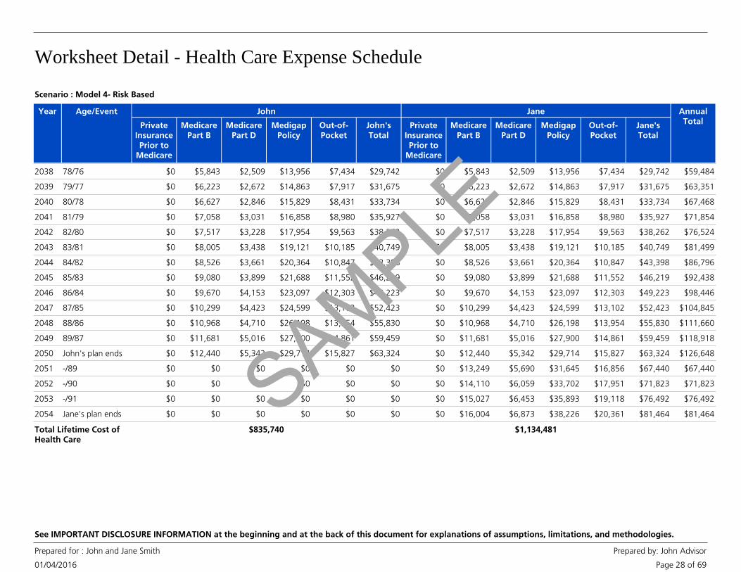
Worksheet Detail - Health Care Expense Schedule
01/04/2016
Prepared for : John and Jane Smith Prepared by: John Advisor
Page 28 of 69
See IMPORTANT DISCLOSURE INFORMATION at the beginning and at the back of this document for explanations of assumptions, limitations, and methodologies.
Year Age/Event John
PrivateInsurancePrior to
Medicare
MedicarePart B
MedicarePart D
MedigapPolicy
Out-of-Pocket
John'sTotal
Jane
PrivateInsurancePrior to
Medicare
MedicarePart B
MedicarePart D
MedigapPolicy
Out-of-Pocket
Jane'sTotal
AnnualTotal
2038 78/76 $0 $5,843 $2,509 $13,956 $7,434 $29,742 $0 $5,843 $2,509 $13,956 $7,434 $29,742 $59,484
2039 79/77 $0 $6,223 $2,672 $14,863 $7,917 $31,675 $0 $6,223 $2,672 $14,863 $7,917 $31,675 $63,351
2040 80/78 $0 $6,627 $2,846 $15,829 $8,431 $33,734 $0 $6,627 $2,846 $15,829 $8,431 $33,734 $67,468
2041 81/79 $0 $7,058 $3,031 $16,858 $8,980 $35,927 $0 $7,058 $3,031 $16,858 $8,980 $35,927 $71,854
2042 82/80 $0 $7,517 $3,228 $17,954 $9,563 $38,262 $0 $7,517 $3,228 $17,954 $9,563 $38,262 $76,524
2043 83/81 $0 $8,005 $3,438 $19,121 $10,185 $40,749 $0 $8,005 $3,438 $19,121 $10,185 $40,749 $81,499
2044 84/82 $0 $8,526 $3,661 $20,364 $10,847 $43,398 $0 $8,526 $3,661 $20,364 $10,847 $43,398 $86,796
2045 85/83 $0 $9,080 $3,899 $21,688 $11,552 $46,219 $0 $9,080 $3,899 $21,688 $11,552 $46,219 $92,438
2046 86/84 $0 $9,670 $4,153 $23,097 $12,303 $49,223 $0 $9,670 $4,153 $23,097 $12,303 $49,223 $98,446
2047 87/85 $0 $10,299 $4,423 $24,599 $13,102 $52,423 $0 $10,299 $4,423 $24,599 $13,102 $52,423 $104,845
2048 88/86 $0 $10,968 $4,710 $26,198 $13,954 $55,830 $0 $10,968 $4,710 $26,198 $13,954 $55,830 $111,660
2049 89/87 $0 $11,681 $5,016 $27,900 $14,861 $59,459 $0 $11,681 $5,016 $27,900 $14,861 $59,459 $118,918
2050 John's plan ends $0 $12,440 $5,342 $29,714 $15,827 $63,324 $0 $12,440 $5,342 $29,714 $15,827 $63,324 $126,648
2051 -/89 $0 $0 $0 $0 $0 $0 $0 $13,249 $5,690 $31,645 $16,856 $67,440 $67,440
2052 -/90 $0 $0 $0 $0 $0 $0 $0 $14,110 $6,059 $33,702 $17,951 $71,823 $71,823
2053 -/91 $0 $0 $0 $0 $0 $0 $0 $15,027 $6,453 $35,893 $19,118 $76,492 $76,492
2054 Jane's plan ends $0 $0 $0 $0 $0 $0 $0 $16,004 $6,873 $38,226 $20,361 $81,464 $81,464
$835,740 $1,134,481Total Lifetime Cost ofHealth Care
Scenario : Model 4- Risk Based
SAMPLE

Worksheet Detail - Health Care Expense Schedule
01/04/2016
Prepared for : John and Jane Smith Prepared by: John Advisor
Page 29 of 69
See IMPORTANT DISCLOSURE INFORMATION at the beginning and at the back of this document for explanations of assumptions, limitations, and methodologies.
Scenario : Model 4- Risk Based
• Program assumptions:
• The scenario assumes that client and co-client will each use a combination of Medicare PartA (Hospital Insurance), Part B (Medical Insurance), Part D (Prescription Drug Insurance),Medigap insurance , and Out-of Pocket expenses. The program uses initial default values thatmay have been adjusted based on your preferences and information provided by you.
Notes
• The scenario assumes that client and co-client each qualify to receive Medicare Part A at nocharge and therefore it is not reflected in the Health Care Expense schedule.
• Estimates for private insurance prior to retirement are based on the information youprovided.
• Medicare and Medigap costs begin at the later of age 65, your retirement age, or thecurrent year.
• All costs are in future dollars.
• Costs associated with Long Term Care needs are not addressed by this goal. A separate LTCgoal can be created.
• General Information regarding Medicare:
• Part B premiums are uniform nationally and are increased for those with a higher ModifiedAdjusted Gross Income.
• Part D coverage is optional. Premiums are increased for those with a higher ModifiedAdjusted Gross Income, differ from state to state, and vary based on the specific plan andlevel of benefit selected.
• Medigap coverage is optional and policies (Plans A-N) are issued by private insurers.
• Clients may incur out-of-pocket healthcare expenses, for costs not covered by Medicarebenefits and Medigap insurance.
• If clients retire before age 65, they may choose to purchase private health insurance or toself-insure. Costs and coverage for private health insurance varies greatly.
SAMPLE
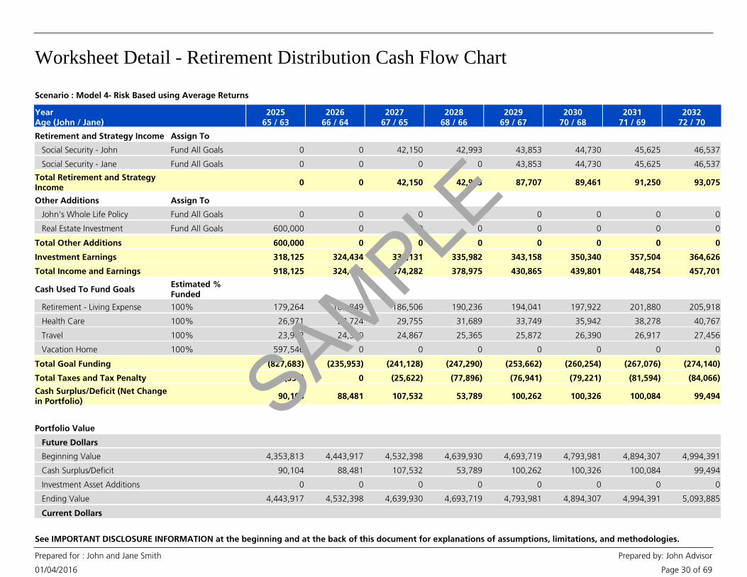
Worksheet Detail - Retirement Distribution Cash Flow Chart
01/04/2016
Prepared for : John and Jane Smith Prepared by: John Advisor
Page 30 of 69
See IMPORTANT DISCLOSURE INFORMATION at the beginning and at the back of this document for explanations of assumptions, limitations, and methodologies.
202565 / 63
202666 / 64
202767 / 65
202868 / 66
202969 / 67
203070 / 68
203171 / 69
203272 / 70
YearAge (John / Jane)
Retirement and Strategy Income Assign To
Social Security - John 0Fund All Goals 0 42,150 42,993 43,853 44,730 45,625 46,537
Social Security - Jane 0Fund All Goals 0 0 0 43,853 44,730 45,625 46,537
Total Retirement and StrategyIncome
0 0 42,150 42,993 87,707 89,461 91,250 93,075
Other Additions Assign To
John's Whole Life Policy 0Fund All Goals 0 0 0 0 0 0 0
Real Estate Investment 600,000Fund All Goals 0 0 0 0 0 0 0
Total Other Additions 600,000 0 0 0 0 0 0 0
Investment Earnings 318,125 324,434 332,131 335,982 343,158 350,340 357,504 364,626
Total Income and Earnings 918,125 324,434 374,282 378,975 430,865 439,801 448,754 457,701
Cash Used To Fund GoalsEstimated %Funded
Retirement - Living Expense 179,264100% 182,849 186,506 190,236 194,041 197,922 201,880 205,918
Health Care 26,971100% 28,724 29,755 31,689 33,749 35,942 38,278 40,767
Travel 23,902100% 24,380 24,867 25,365 25,872 26,390 26,917 27,456
Vacation Home 597,546100% 0 0 0 0 0 0 0
Total Goal Funding (827,683) (235,953) (241,128) (247,290) (253,662) (260,254) (267,076) (274,140)
Total Taxes and Tax Penalty (338) 0 (25,622) (77,896) (76,941) (79,221) (81,594) (84,066)
Cash Surplus/Deficit (Net Changein Portfolio)
90,104 88,481 107,532 53,789 100,262 100,326 100,084 99,494
Portfolio Value
Future Dollars
Beginning Value 4,353,813 4,443,917 4,532,398 4,639,930 4,693,719 4,793,981 4,894,307 4,994,391
Cash Surplus/Deficit 90,104 88,481 107,532 53,789 100,262 100,326 100,084 99,494
Investment Asset Additions 0 0 0 0 0 0 0 0
Ending Value 4,443,917 4,532,398 4,639,930 4,693,719 4,793,981 4,894,307 4,994,391 5,093,885
Current Dollars
Scenario : Model 4- Risk Based using Average Returns
SAMPLE
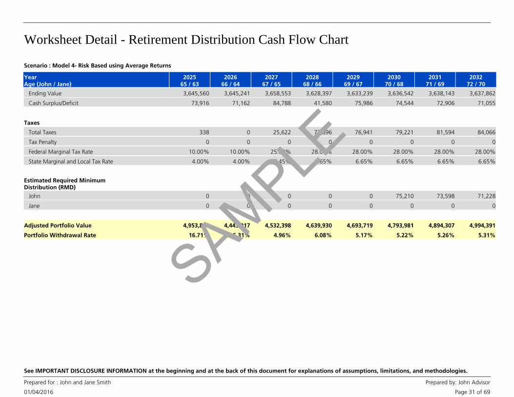
Worksheet Detail - Retirement Distribution Cash Flow Chart
01/04/2016
Prepared for : John and Jane Smith Prepared by: John Advisor
Page 31 of 69
See IMPORTANT DISCLOSURE INFORMATION at the beginning and at the back of this document for explanations of assumptions, limitations, and methodologies.
202565 / 63
202666 / 64
202767 / 65
202868 / 66
202969 / 67
203070 / 68
203171 / 69
203272 / 70
YearAge (John / Jane)
Ending Value 3,645,560 3,645,241 3,658,553 3,628,397 3,633,239 3,636,542 3,638,143 3,637,862
Cash Surplus/Deficit 73,916 71,162 84,788 41,580 75,986 74,544 72,906 71,055
Taxes
Total Taxes 338 0 25,622 77,896 76,941 79,221 81,594 84,066
Tax Penalty 0 0 0 0 0 0 0 0
Federal Marginal Tax Rate 10.00% 10.00% 25.00% 28.00% 28.00% 28.00% 28.00% 28.00%
State Marginal and Local Tax Rate 4.00% 4.00% 6.45% 6.65% 6.65% 6.65% 6.65% 6.65%
Estimated Required MinimumDistribution (RMD)
John 0 0 0 0 0 75,210 73,598 71,228
Jane 0 0 0 0 0 0 0 0
Adjusted Portfolio Value 4,953,813 4,443,917 4,532,398 4,639,930 4,693,719 4,793,981 4,894,307 4,994,391
Portfolio Withdrawal Rate 16.71% 5.31% 4.96% 6.08% 5.17% 5.22% 5.26% 5.31%
Scenario : Model 4- Risk Based using Average Returns
SAMPLE
Worksheet Detail - Retirement Distribution Cash Flow Chart
01/04/2016
Prepared for : John and Jane Smith Prepared by: John Advisor
Page 32 of 69
See IMPORTANT DISCLOSURE INFORMATION at the beginning and at the back of this document for explanations of assumptions, limitations, and methodologies.
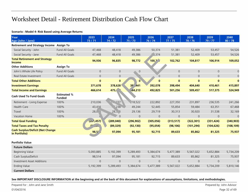
203373 / 71
203474 / 72
203575 / 73
203676 / 74
203777 / 75
203878 / 76
203979 / 77
204080 / 78
YearAge (John / Jane)
Retirement and Strategy Income Assign To
Social Security - John 47,468Fund All Goals 48,418 49,386 50,374 51,381 52,409 53,457 54,526
Social Security - Jane 47,468Fund All Goals 48,418 49,386 50,374 51,381 52,409 53,457 54,526
Total Retirement and StrategyIncome
94,936 96,835 98,772 100,747 102,762 104,817 106,914 109,052
Other Additions Assign To
John's Whole Life Policy 0Fund All Goals 0 0 0 0 0 0 0
Real Estate Investment 0Fund All Goals 0 0 0 0 0 0 0
Total Other Additions 0 0 0 0 0 0 0 0
Investment Earnings 371,678 378,628 385,441 392,078 398,494 404,640 410,461 415,897
Total Income and Earnings 466,614 475,463 484,213 492,825 501,256 509,457 517,375 524,949
Cash Used To Fund GoalsEstimated %Funded
Retirement - Living Expense 210,036100% 214,237 218,522 222,892 227,350 231,897 236,535 241,266
Health Care 43,416100% 46,238 49,244 52,445 55,854 59,484 63,351 67,468
Travel 28,005100% 28,565 29,136 29,719 30,313 30,920 31,538 32,169
Vacation Home 0100% 0 0 0 0 0 0 0
Total Goal Funding (281,457) (289,040) (296,902) (305,056) (313,517) (322,301) (331,424) (340,903)
Total Taxes and Tax Penalty (86,643) (89,329) (92,130) (95,054) (98,106) (101,294) (104,626) (108,109)
Cash Surplus/Deficit (Net Changein Portfolio)
98,514 97,094 95,181 92,715 89,633 85,862 81,325 75,937
Portfolio Value
Future Dollars
Beginning Value 5,093,885 5,192,399 5,289,493 5,384,674 5,477,389 5,567,022 5,652,884 5,734,209
Cash Surplus/Deficit 98,514 97,094 95,181 92,715 89,633 85,862 81,325 75,937
Investment Asset Additions 0 0 0 0 0 0 0 0
Ending Value 5,192,399 5,289,493 5,384,674 5,477,389 5,567,022 5,652,884 5,734,209 5,810,146
Current Dollars
Scenario : Model 4- Risk Based using Average Returns
SAMPLE

Worksheet Detail - Retirement Distribution Cash Flow Chart
01/04/2016
Prepared for : John and Jane Smith Prepared by: John Advisor
Page 33 of 69
See IMPORTANT DISCLOSURE INFORMATION at the beginning and at the back of this document for explanations of assumptions, limitations, and methodologies.
203373 / 71
203474 / 72
203575 / 73
203676 / 74
203777 / 75
203878 / 76
203979 / 77
204080 / 78
YearAge (John / Jane)
Ending Value 3,635,507 3,630,871 3,623,731 3,613,849 3,600,967 3,584,810 3,565,081 3,541,463
Cash Surplus/Deficit 68,976 66,648 64,054 61,171 57,978 54,450 50,562 46,286
Taxes
Total Taxes 86,643 89,329 92,130 95,054 98,106 101,294 104,626 108,109
Tax Penalty 0 0 0 0 0 0 0 0
Federal Marginal Tax Rate 28.00% 28.00% 28.00% 28.00% 28.00% 28.00% 28.00% 28.00%
State Marginal and Local Tax Rate 6.65% 6.65% 6.65% 6.65% 6.65% 6.65% 6.65% 6.65%
Estimated Required MinimumDistribution (RMD)
John 67,954 69,431 70,986 72,638 74,065 75,977 77,689 79,544
Jane 128,884 138,279 148,337 159,102 170,621 182,940 195,186 209,199
Adjusted Portfolio Value 5,093,885 5,192,399 5,289,493 5,384,674 5,477,389 5,567,022 5,652,884 5,734,209
Portfolio Withdrawal Rate 5.36% 5.42% 5.49% 5.56% 5.64% 5.73% 5.82% 5.93%
Scenario : Model 4- Risk Based using Average Returns
SAMPLE
Worksheet Detail - Retirement Distribution Cash Flow Chart
01/04/2016
Prepared for : John and Jane Smith Prepared by: John Advisor
Page 34 of 69
See IMPORTANT DISCLOSURE INFORMATION at the beginning and at the back of this document for explanations of assumptions, limitations, and methodologies.
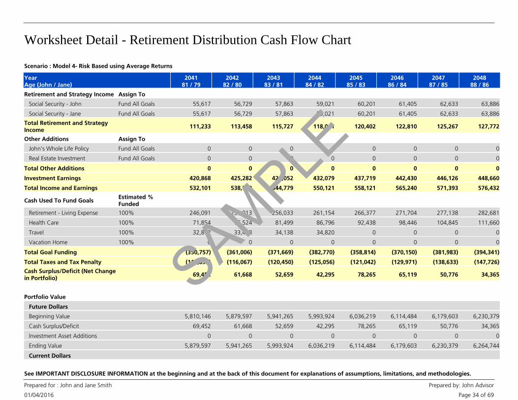
204181 / 79
204282 / 80
204383 / 81
204484 / 82
204585 / 83
204686 / 84
204787 / 85
204888 / 86
YearAge (John / Jane)
Retirement and Strategy Income Assign To
Social Security - John 55,617Fund All Goals 56,729 57,863 59,021 60,201 61,405 62,633 63,886
Social Security - Jane 55,617Fund All Goals 56,729 57,863 59,021 60,201 61,405 62,633 63,886
Total Retirement and StrategyIncome
111,233 113,458 115,727 118,041 120,402 122,810 125,267 127,772
Other Additions Assign To
John's Whole Life Policy 0Fund All Goals 0 0 0 0 0 0 0
Real Estate Investment 0Fund All Goals 0 0 0 0 0 0 0
Total Other Additions 0 0 0 0 0 0 0 0
Investment Earnings 420,868 425,282 429,052 432,079 437,719 442,430 446,126 448,660
Total Income and Earnings 532,101 538,740 544,779 550,121 558,121 565,240 571,393 576,432
Cash Used To Fund GoalsEstimated %Funded
Retirement - Living Expense 246,091100% 251,013 256,033 261,154 266,377 271,704 277,138 282,681
Health Care 71,854100% 76,524 81,499 86,796 92,438 98,446 104,845 111,660
Travel 32,812100% 33,468 34,138 34,820 0 0 0 0
Vacation Home 0100% 0 0 0 0 0 0 0
Total Goal Funding (350,757) (361,006) (371,669) (382,770) (358,814) (370,150) (381,983) (394,341)
Total Taxes and Tax Penalty (111,893) (116,067) (120,450) (125,056) (121,042) (129,971) (138,633) (147,726)
Cash Surplus/Deficit (Net Changein Portfolio)
69,452 61,668 52,659 42,295 78,265 65,119 50,776 34,365
Portfolio Value
Future Dollars
Beginning Value 5,810,146 5,879,597 5,941,265 5,993,924 6,036,219 6,114,484 6,179,603 6,230,379
Cash Surplus/Deficit 69,452 61,668 52,659 42,295 78,265 65,119 50,776 34,365
Investment Asset Additions 0 0 0 0 0 0 0 0
Ending Value 5,879,597 5,941,265 5,993,924 6,036,219 6,114,484 6,179,603 6,230,379 6,264,744
Current Dollars
Scenario : Model 4- Risk Based using Average Returns
SAMPLE
Worksheet Detail - Retirement Distribution Cash Flow Chart
01/04/2016
Prepared for : John and Jane Smith Prepared by: John Advisor
Page 35 of 69
See IMPORTANT DISCLOSURE INFORMATION at the beginning and at the back of this document for explanations of assumptions, limitations, and methodologies.
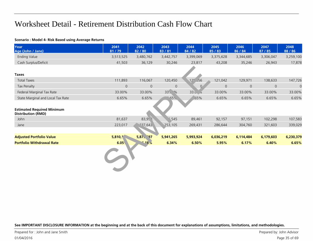
204181 / 79
204282 / 80
204383 / 81
204484 / 82
204585 / 83
204686 / 84
204787 / 85
204888 / 86
YearAge (John / Jane)
Ending Value 3,513,525 3,480,762 3,442,757 3,399,069 3,375,628 3,344,685 3,306,047 3,259,100
Cash Surplus/Deficit 41,503 36,129 30,246 23,817 43,208 35,246 26,943 17,878
Taxes
Total Taxes 111,893 116,067 120,450 125,056 121,042 129,971 138,633 147,726
Tax Penalty 0 0 0 0 0 0 0 0
Federal Marginal Tax Rate 33.00% 33.00% 33.00% 33.00% 33.00% 33.00% 33.00% 33.00%
State Marginal and Local Tax Rate 6.65% 6.65% 6.65% 6.65% 6.65% 6.65% 6.65% 6.65%
Estimated Required MinimumDistribution (RMD)
John 81,637 83,958 86,545 89,461 92,157 97,151 102,298 107,583
Jane 223,017 237,643 253,105 269,431 286,644 304,760 321,603 339,029
Adjusted Portfolio Value 5,810,146 5,879,597 5,941,265 5,993,924 6,036,219 6,114,484 6,179,603 6,230,379
Portfolio Withdrawal Rate 6.05% 6.18% 6.34% 6.50% 5.95% 6.17% 6.40% 6.65%
Scenario : Model 4- Risk Based using Average Returns
SAMPLE
Worksheet Detail - Retirement Distribution Cash Flow Chart
01/04/2016
Prepared for : John and Jane Smith Prepared by: John Advisor
Page 36 of 69
See IMPORTANT DISCLOSURE INFORMATION at the beginning and at the back of this document for explanations of assumptions, limitations, and methodologies.
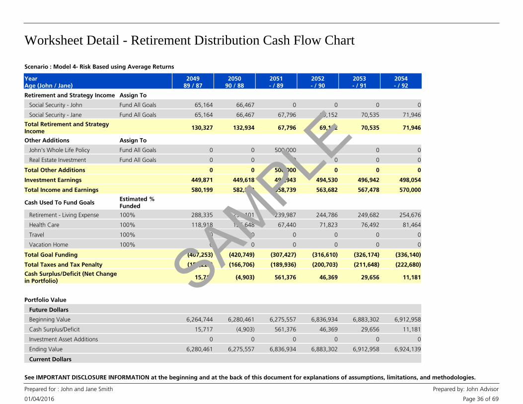
204989 / 87
205090 / 88
2051- / 89
2052- / 90
2053- / 91
2054- / 92
YearAge (John / Jane)
Retirement and Strategy Income Assign To
Social Security - John 65,164Fund All Goals 66,467 0 0 0 0
Social Security - Jane 65,164Fund All Goals 66,467 67,796 69,152 70,535 71,946
Total Retirement and StrategyIncome
130,327 132,934 67,796 69,152 70,535 71,946
Other Additions Assign To
John's Whole Life Policy 0Fund All Goals 0 500,000 0 0 0
Real Estate Investment 0Fund All Goals 0 0 0 0 0
Total Other Additions 0 0 500,000 0 0 0
Investment Earnings 449,871 449,618 490,943 494,530 496,942 498,054
Total Income and Earnings 580,199 582,552 1,058,739 563,682 567,478 570,000
Cash Used To Fund GoalsEstimated %Funded
Retirement - Living Expense 288,335100% 294,101 239,987 244,786 249,682 254,676
Health Care 118,918100% 126,648 67,440 71,823 76,492 81,464
Travel 0100% 0 0 0 0 0
Vacation Home 0100% 0 0 0 0 0
Total Goal Funding (407,253) (420,749) (307,427) (316,610) (326,174) (336,140)
Total Taxes and Tax Penalty (157,229) (166,706) (189,936) (200,703) (211,648) (222,680)
Cash Surplus/Deficit (Net Changein Portfolio)
15,717 (4,903) 561,376 46,369 29,656 11,181
Portfolio Value
Future Dollars
Beginning Value 6,264,744 6,280,461 6,275,557 6,836,934 6,883,302 6,912,958
Cash Surplus/Deficit 15,717 (4,903) 561,376 46,369 29,656 11,181
Investment Asset Additions 0 0 0 0 0 0
Ending Value 6,280,461 6,275,557 6,836,934 6,883,302 6,912,958 6,924,139
Current Dollars
Scenario : Model 4- Risk Based using Average Returns
SAMPLE
Worksheet Detail - Retirement Distribution Cash Flow Chart
01/04/2016
Prepared for : John and Jane Smith Prepared by: John Advisor
Page 37 of 69
See IMPORTANT DISCLOSURE INFORMATION at the beginning and at the back of this document for explanations of assumptions, limitations, and methodologies.
204989 / 87
205090 / 88
2051- / 89
2052- / 90
2053- / 91
2054- / 92
YearAge (John / Jane)
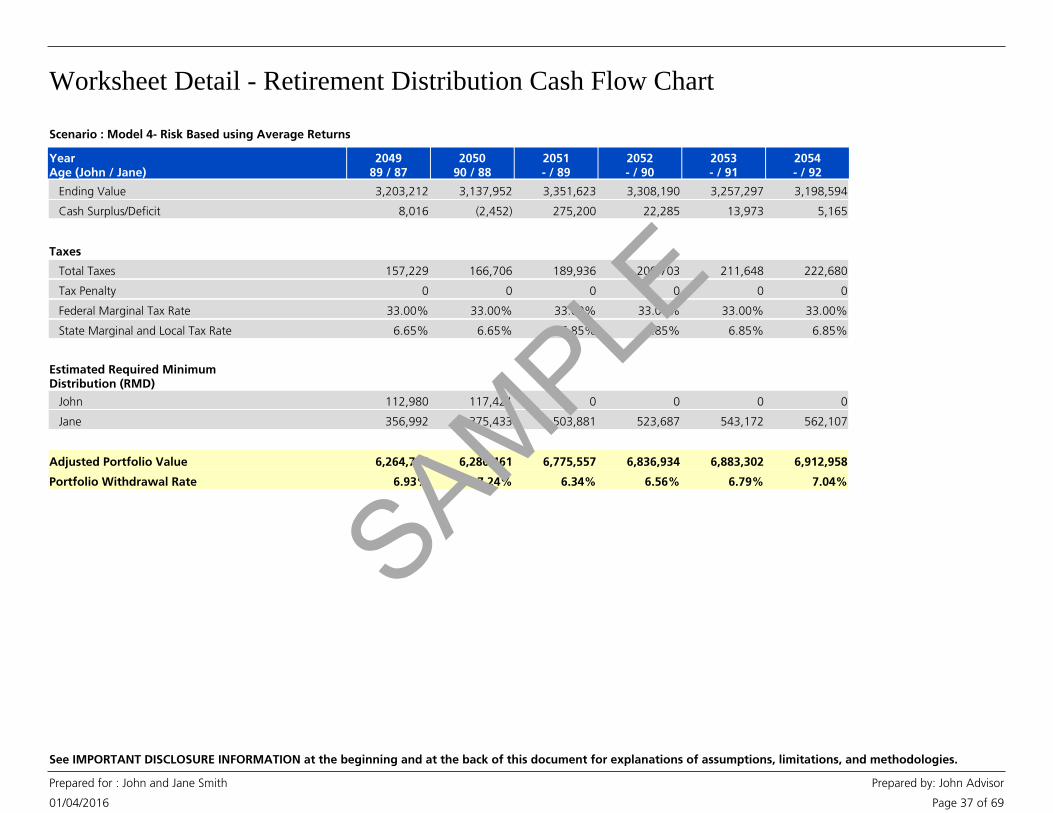
Ending Value 3,203,212 3,137,952 3,351,623 3,308,190 3,257,297 3,198,594
Cash Surplus/Deficit 8,016 (2,452) 275,200 22,285 13,973 5,165
Taxes
Total Taxes 157,229 166,706 189,936 200,703 211,648 222,680
Tax Penalty 0 0 0 0 0 0
Federal Marginal Tax Rate 33.00% 33.00% 33.00% 33.00% 33.00% 33.00%
State Marginal and Local Tax Rate 6.65% 6.65% 6.85% 6.85% 6.85% 6.85%
Estimated Required MinimumDistribution (RMD)
John 112,980 117,421 0 0 0 0
Jane 356,992 375,433 503,881 523,687 543,172 562,107
Adjusted Portfolio Value 6,264,744 6,280,461 6,775,557 6,836,934 6,883,302 6,912,958
Portfolio Withdrawal Rate 6.93% 7.24% 6.34% 6.56% 6.79% 7.04%
Scenario : Model 4- Risk Based using Average Returns
SAMPLE
Worksheet Detail - Retirement Distribution Cash Flow Chart
01/04/2016
Prepared for : John and Jane Smith Prepared by: John Advisor
Page 38 of 69
See IMPORTANT DISCLOSURE INFORMATION at the beginning and at the back of this document for explanations of assumptions, limitations, and methodologies.
Scenario : Model 4- Risk Based using Average Returns
• For married clients, if either Social Security Program Estimate or Use This Amount andEvaluate Annually is selected for a participant, the Program defaults to the greater of theselected benefit or the age-adjusted spousal benefit based on the other participant’sbenefit. The spousal benefit is not applicable to domestic partners.
• The Income section includes Retirement Income, Strategy Income, Stock Options,Restricted Stock, Other Assets, proceeds from Insurance Policies, and any remaining assetvalue after 72(t) distributions have been completed.
• Retirement Income includes the following: Social Security, pension, annuity, rentalproperty, royalty, alimony, part-time employment, trust, and any other retirement income asentered in the Scenario.
• Additions and withdrawals occur at the beginning of the year.
• Results may vary with use and over time.
• IMPORTANT: The projections or other information generated by this tool regarding thelikelihood of various investment outcomes are hypothetical in nature, do not reflect actualinvestment results, and are not guarantees of future results.
• The return assumptions used are estimates based on average annual returns for the indexused as a proxy for each asset class. The portfolio returns were calculated by weightingindividual return assumptions for each asset class according to the portfolio allocationselected by you or your Financial Advisor. The portfolio returns may have also been modifiedby your Financial Advisor to reflect the outcome of a different return by conducting a TotalReturn Adjustment or selecting a Custom Portfolio. For a explanation of the methodologyused to calculate returns, please review the Important Disclosure Information and ReturnMethodology sections.
• The return assumptions in this tool are not reflective of any specific product and do notinclude any fees or expenses that may be incurred by investing in specific products. Theactual returns of a specific product may be more or less than the returns used in this tool.
• No investment strategy or allocation can eliminate risk or guarantee investment results.
• The values shown for income and investment earnings are estimates based on theassumptions included in this report, such as rates of return, inflation rate, asset values, assetadditions, tax rates, income sources and amounts, and goal expenses. Any changes inassumptions will also change these values.
• Strategy Income is based on the particulars of the Goal Strategies selected. StrategyIncome from immediate annuities and 72(t) distributions is pre-tax. Strategy Income fromNet Unrealized Appreciation (NUA) is after-tax.
Notes
• Stock Options and Restricted Stock values are after-tax and based on the Exercise Scenarioselected.
• Income from Other Assets and proceeds from Insurance Policies are after-tax values. Anyremaining asset value after 72(t) distributions have been completed is a pre-tax value.
• Investment Earnings are calculated on all assets after any withdrawals for funding Goals,taxes on withdrawals, and tax penalties, if applicable, are subtracted.
• Shortfalls that occur in a particular year are denoted with an 'x' in the Cash Used to FundGoals section of the chart.
• The Total Taxes are a sum of (1) taxes on retirement income, (2) taxes on strategy income,(3) taxes on withdrawals from qualified assets for Required Minimum Distributions, (4) taxeson withdrawals from taxable assets' untaxed gain used to fund Goals in that year, (5) taxeson withdrawals from tax-deferred or qualified assets used to fund Goals in that year, and (6)taxes on the investment earnings of taxable assets. Tax rates used are detailed in the Taxand Inflation Options page. (Please note, the Total Taxes do not include any taxes owedfrom the exercise of Stock Options or the vesting of Restricted Stock.)
• Tax Penalties can occur when Qualified and Tax-Deferred Assets are used prior to age59½. If there is a value in this row, it illustrates that you are using your assets in thisScenario in a manner that may incur tax penalties. Generally, it is better to avoid taxpenalties whenever possible.
• The Cash Surplus/Deficit is the net change in the Portfolio Value for the specified year.This value is your income and earnings minus what was spent to fund Goals minus taxes.
• The Ending Value of the Portfolio in Current Dollars is calculated by discounting theEnding Value of the Portfolio in Future Dollars by the Base Inflation Rate for this Scenario.
• The Cash Surplus/Deficit in Current Dollars is calculated by discounting the CashSurplus/Deficit in Future Dollars by the Base Inflation Rate for this Scenario.
• These calculations do not incorporate penalties associated with use of 529 Planwithdrawals for non-qualified expenses.
• For married clients, ownership of qualified assets is assumed to roll over to the survivingco-client at the death of the original owner. For domestic partners, qualified assets areassumed to be transferred as a non-spousal inheritance to the surviving co-client at thedeath of the original owner. In both cases, the Program assumes the surviving co-clientinherits all remaining assets of the original owner.
SAMPLE
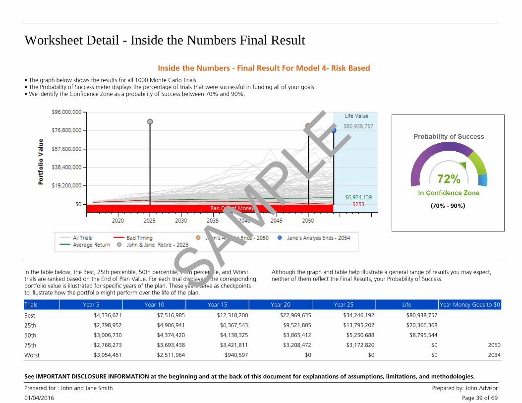
Worksheet Detail - Inside the Numbers Final Result
01/04/2016
Prepared for : John and Jane Smith Prepared by: John Advisor
Page 39 of 69
See IMPORTANT DISCLOSURE INFORMATION at the beginning and at the back of this document for explanations of assumptions, limitations, and methodologies.
• The graph below shows the results for all 1000 Monte Carlo Trials.• The Probability of Success meter displays the percentage of trials that were successful in funding all of your goals.• We identify the Confidence Zone as a probability of Success between 70% and 90%.
(70% - 90%)
In the table below, the Best, 25th percentile, 50th percentile, 75th percentile, and Worsttrials are ranked based on the End of Plan Value. For each trial displayed, the correspondingportfolio value is illustrated for specific years of the plan. These years serve as checkpointsto illustrate how the portfolio might perform over the life of the plan.
Although the graph and table help illustrate a general range of results you may expect,neither of them reflect the Final Results, your Probability of Success.
Trials Year 5 Year 10 Year 15 Year 20 Year 25 Life Year Money Goes to $0
Best $4,336,621 $7,516,985 $12,318,200 $22,969,635 $34,246,192 $80,938,757
25th $2,798,952 $4,906,941 $6,367,543 $9,521,805 $13,795,202 $20,366,368
50th $3,006,730 $4,374,420 $4,138,325 $3,865,412 $5,250,688 $8,795,544
75th $2,768,273 $3,693,438 $3,421,811 $3,208,472 $3,172,820 $0 2050
Worst $3,054,451 $2,511,964 $940,597 $0 $0 $0 2034
Inside the Numbers - Final Result For Model 4- Risk Based
SAMPLE
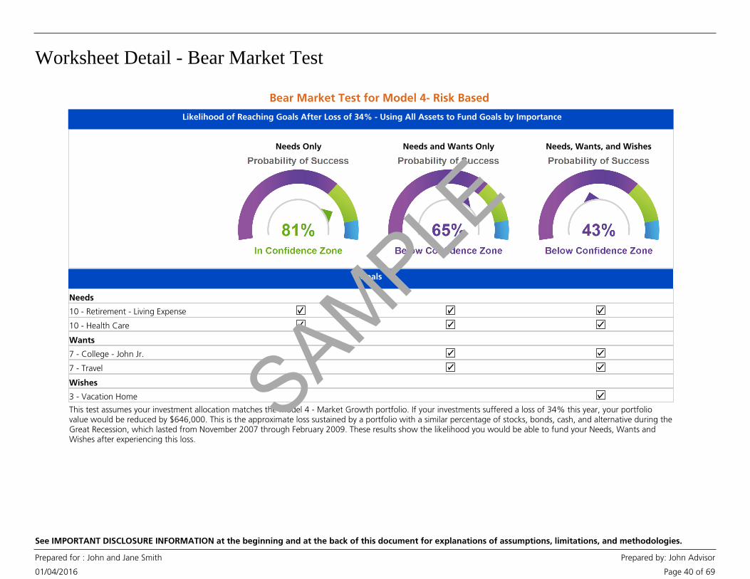
Worksheet Detail - Bear Market Test
01/04/2016
Prepared for : John and Jane Smith Prepared by: John Advisor
Page 40 of 69
See IMPORTANT DISCLOSURE INFORMATION at the beginning and at the back of this document for explanations of assumptions, limitations, and methodologies.
Likelihood of Reaching Goals After Loss of 34% - Using All Assets to Fund Goals by Importance
Needs, Wants, and WishesNeeds and Wants OnlyNeeds Only
Goals
Needs
10 - Retirement - Living Expense
10 - Health Care
Wants
7 - College - John Jr.
7 - Travel
Wishes
3 - Vacation Home
This test assumes your investment allocation matches the Model 4 - Market Growth portfolio. If your investments suffered a loss of 34% this year, your portfoliovalue would be reduced by $646,000. This is the approximate loss sustained by a portfolio with a similar percentage of stocks, bonds, cash, and alternative during theGreat Recession, which lasted from November 2007 through February 2009. These results show the likelihood you would be able to fund your Needs, Wants andWishes after experiencing this loss.
Bear Market Test for Model 4- Risk Based
SAMPLE
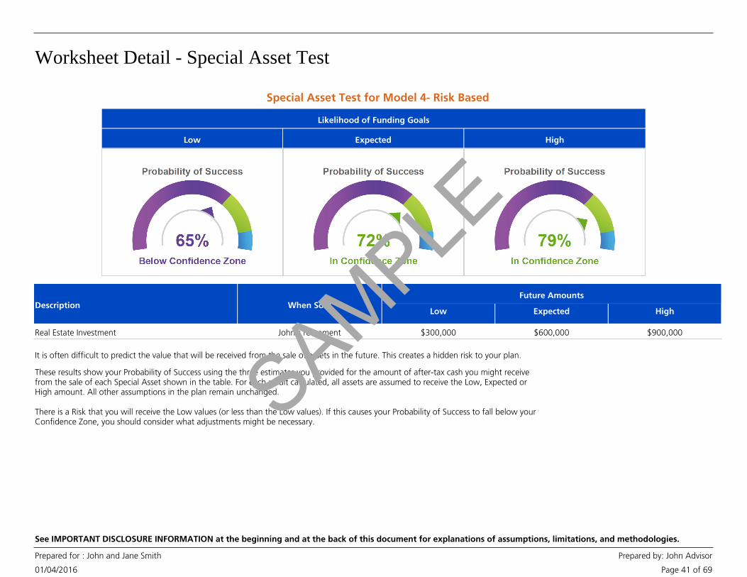
Worksheet Detail - Special Asset Test
01/04/2016
Prepared for : John and Jane Smith Prepared by: John Advisor
Page 41 of 69
See IMPORTANT DISCLOSURE INFORMATION at the beginning and at the back of this document for explanations of assumptions, limitations, and methodologies.
Likelihood of Funding Goals
Low Expected High
Description When SoldLow Expected High
Future Amounts
$600,000$300,000John's retirementReal Estate Investment $900,000
It is often difficult to predict the value that will be received from the sale of assets in the future. This creates a hidden risk to your plan.
These results show your Probability of Success using the three estimates you provided for the amount of after-tax cash you might receivefrom the sale of each Special Asset shown in the table. For each result calculated, all assets are assumed to receive the Low, Expected orHigh amount. All other assumptions in the plan remain unchanged.
There is a Risk that you will receive the Low values (or less than the Low values). If this causes your Probability of Success to fall below yourConfidence Zone, you should consider what adjustments might be necessary.
Special Asset Test for Model 4- Risk Based
SAMPLE
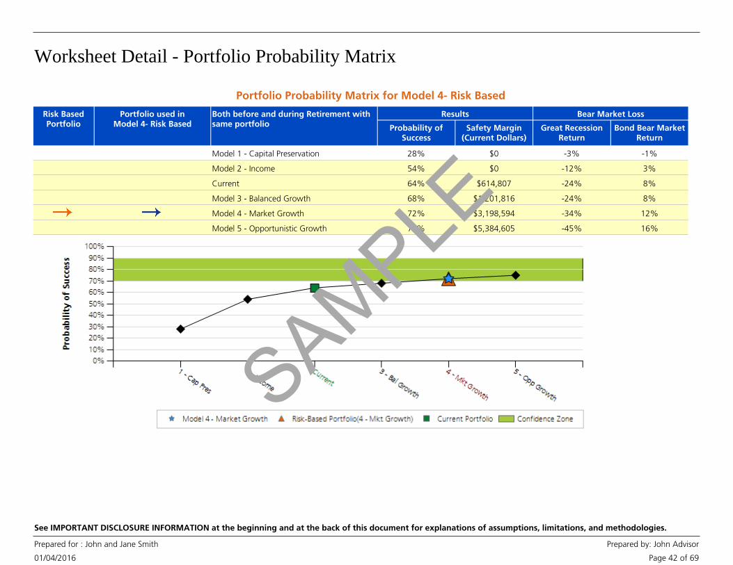
Worksheet Detail - Portfolio Probability Matrix
01/04/2016
Prepared for : John and Jane Smith Prepared by: John Advisor
Page 42 of 69
See IMPORTANT DISCLOSURE INFORMATION at the beginning and at the back of this document for explanations of assumptions, limitations, and methodologies.
Risk BasedPortfolio
Both before and during Retirement withsame portfolio Probability of
SuccessGreat Recession
Return
Portfolio used inModel 4- Risk Based Safety Margin
(Current Dollars)Bond Bear Market
Return
Results Bear Market Loss
-3%28%Model 1 - Capital Preservation $0 -1%
-12%54%Model 2 - Income $0 3%
-24%64%Current $614,807 8%
-24%68%Model 3 - Balanced Growth $1,201,816 8%
-34%72%Model 4 - Market Growth $3,198,594 12%
-45%75%Model 5 - Opportunistic Growth $5,384,605 16%
Portfolio Probability Matrix for Model 4- Risk Based
SAMPLE
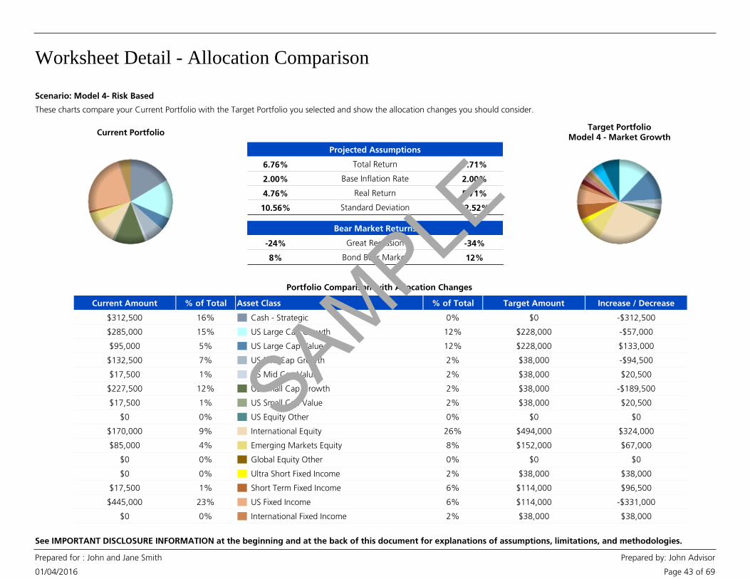
Worksheet Detail - Allocation Comparison
01/04/2016
Prepared for : John and Jane Smith Prepared by: John Advisor
Page 43 of 69
See IMPORTANT DISCLOSURE INFORMATION at the beginning and at the back of this document for explanations of assumptions, limitations, and methodologies.
Current Portfolio
These charts compare your Current Portfolio with the Target Portfolio you selected and show the allocation changes you should consider.
Target PortfolioModel 4 - Market Growth
Projected Assumptions
6.76% Total Return 7.71%
2.00% Base Inflation Rate 2.00%
4.76% Real Return 5.71%
10.56% Standard Deviation 12.52%
Bear Market Returns
-24% Great Recession -34%
8% Bond Bear Market 12%
Asset Class % of Total Target AmountCurrent Amount % of Total
Portfolio Comparison with Allocation Changes
Increase / Decrease
Cash - Strategic 0% $016%$312,500 -$312,500
US Large Cap Growth 12% $228,00015%$285,000 -$57,000
US Large Cap Value 12% $228,0005%$95,000 $133,000
US Mid Cap Growth 2% $38,0007%$132,500 -$94,500
US Mid Cap Value 2% $38,0001%$17,500 $20,500
US Small Cap Growth 2% $38,00012%$227,500 -$189,500
US Small Cap Value 2% $38,0001%$17,500 $20,500
US Equity Other 0% $00%$0 $0
International Equity 26% $494,0009%$170,000 $324,000
Emerging Markets Equity 8% $152,0004%$85,000 $67,000
Global Equity Other 0% $00%$0 $0
Ultra Short Fixed Income 2% $38,0000%$0 $38,000
Short Term Fixed Income 6% $114,0001%$17,500 $96,500
US Fixed Income 6% $114,00023%$445,000 -$331,000
International Fixed Income 2% $38,0000%$0 $38,000
Scenario: Model 4- Risk Based
SAMPLE
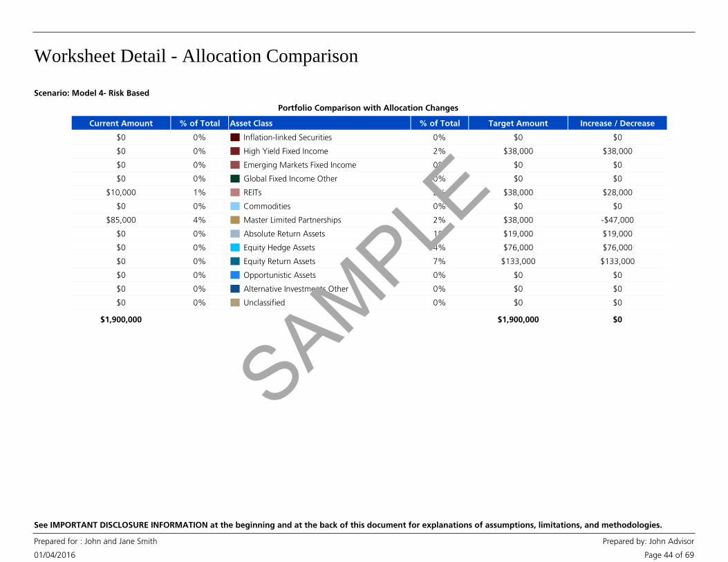
Worksheet Detail - Allocation Comparison
01/04/2016
Prepared for : John and Jane Smith Prepared by: John Advisor
Page 44 of 69
See IMPORTANT DISCLOSURE INFORMATION at the beginning and at the back of this document for explanations of assumptions, limitations, and methodologies.
Asset Class % of Total Target AmountCurrent Amount % of Total
Portfolio Comparison with Allocation Changes
Increase / Decrease
Inflation-linked Securities 0% $00%$0 $0
High Yield Fixed Income 2% $38,0000%$0 $38,000
Emerging Markets Fixed Income 0% $00%$0 $0
Global Fixed Income Other 0% $00%$0 $0
REITs 2% $38,0001%$10,000 $28,000
Commodities 0% $00%$0 $0
Master Limited Partnerships 2% $38,0004%$85,000 -$47,000
Absolute Return Assets 1% $19,0000%$0 $19,000
Equity Hedge Assets 4% $76,0000%$0 $76,000
Equity Return Assets 7% $133,0000%$0 $133,000
Opportunistic Assets 0% $00%$0 $0
Alternative Investments Other 0% $00%$0 $0
Unclassified 0% $00%$0 $0
$1,900,000 $1,900,000 $0
Scenario: Model 4- Risk Based
SAMPLE
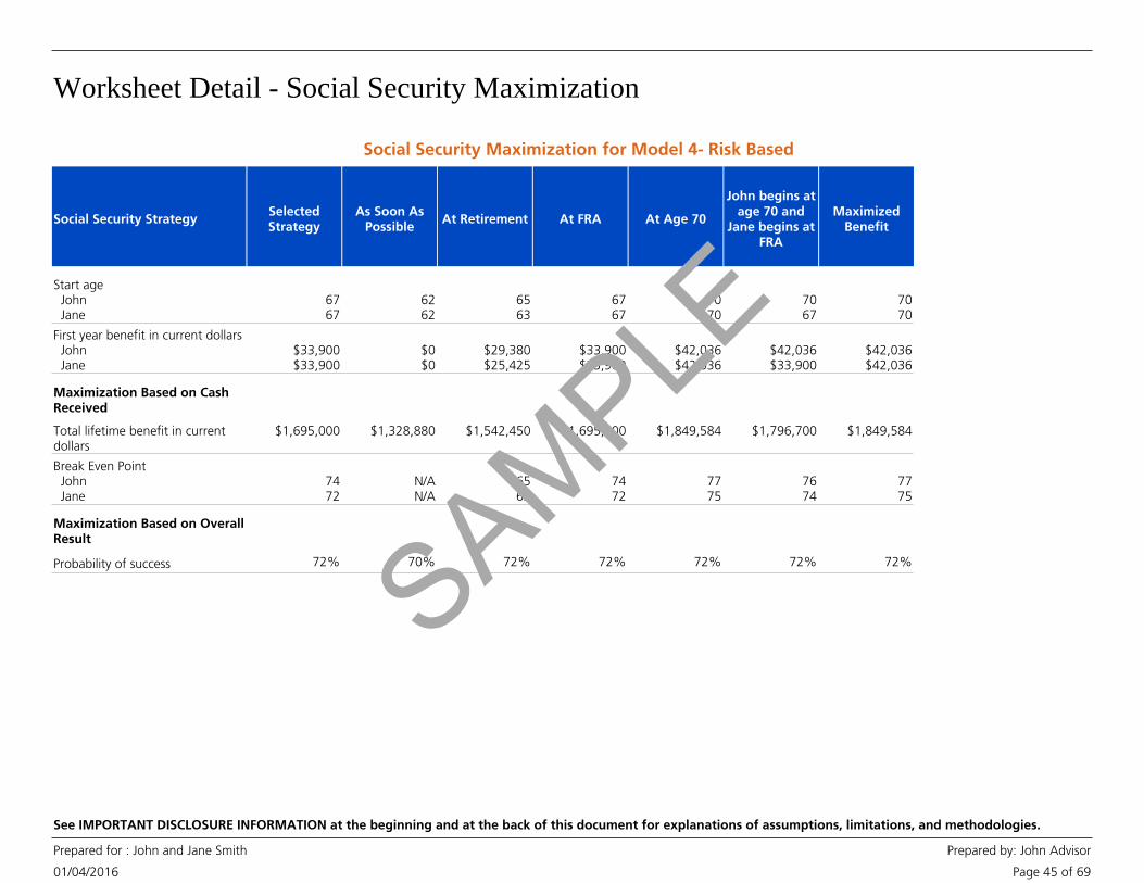
Worksheet Detail - Social Security Maximization
01/04/2016
Prepared for : John and Jane Smith Prepared by: John Advisor
Page 45 of 69
See IMPORTANT DISCLOSURE INFORMATION at the beginning and at the back of this document for explanations of assumptions, limitations, and methodologies.
As Soon AsPossible
At Retirement At FRA At Age 70
John begins atage 70 and
Jane begins atFRA
MaximizedBenefit
SelectedStrategy
Social Security Strategy
Start age John Jane
6767
6262
6563
6767
7070
7067
7070
First year benefit in current dollars John Jane
$33,900$33,900
$0$0
$29,380$25,425
$33,900$33,900
$42,036$42,036
$42,036$33,900
$42,036$42,036
Maximization Based on CashReceived
Total lifetime benefit in currentdollars
$1,695,000 $1,328,880 $1,542,450 $1,695,000 $1,849,584 $1,796,700 $1,849,584
Break Even Point John Jane
7472
N/AN/A
6563
7472
7775
7674
7775
Maximization Based on OverallResult
Probability of success 72% 70% 72% 72% 72% 72% 72%
Social Security Maximization for Model 4- Risk Based
SAMPLE

Worksheet Detail - Social Security Maximization
01/04/2016
Prepared for : John and Jane Smith Prepared by: John Advisor
Page 46 of 69
See IMPORTANT DISCLOSURE INFORMATION at the beginning and at the back of this document for explanations of assumptions, limitations, and methodologies.
Social Security Maximization for Model 4- Risk Based
Notes
Selected Strategy:
You apply for and begin benefits at the later of your current age or age 62. The benefit isautomatically adjusted to account for excess earnings from part-time work, if applicable, andtaking benefits prior to your FRA. If you are age 62 or older, this option is not available.
This strategy is available only if you are married. The higher wage earner applies for and beginsbenefits at age 70. The lower wage earner applies for and begins benefits at his/her FRA. Thehigher/lower wage earners are determined based on the employment incomes you specified.
This strategy is available only if you are married. The lower wage earner applies for and suspendstaking benefits until age 70. The lower wage earner can file at or after his/her FRA, at which timethe spouse (the higher wage earner) files for and takes spousal benefits. The spouse then files forand begins his/her own benefit at age 70, at the higher benefit amount.
The higher wage earner makes a restricted application at his/her FRA. Restricted applicationallows the account holder to apply only for the "spousal benefit" s/he would be due under dualentitlement rules. At any age beyond his/her FRA, the higher wage earner can apply for andreceive benefits based on his/her own work history.
This is the strategy you selected.
At FRA:
You apply for and begin retirement benefits at your Full Retirement Age (FRA), which isdetermined by your date of birth. If the retirement age you specified is after your FRA, weassume you will begin benefits at FRA, and we will adjust the benefit for inflation until yourretirement age.
At Retirement:
You apply for and begin retirement benefits at the retirement age shown. The benefit isautomatically adjusted to account for excess earnings from part-time work and/or taking benefitsprior to your FRA, if either is applicable.
As soon as possible:
At age 70:
You apply for and begin benefits at age 70.
(Higher Wage Earner) begins at age 70 and (Lower Wage Earner) begins at FRA:
The lower wage earner makes a restricted application at his/her FRA. Restricted application allowsthe account holder to apply only for the "spousal benefit" s/he would be due under dualentitlement rules. At any age beyond his/her FRA, the lower wage earner can apply for andreceive benefits based on his/her own work history.
(Lower Wage Earner) files/suspends and (Higher Wage Earner) restricted application:
Maximized Benefits:
This is the strategy that provides the highest estimate of lifetime Social Security income, assumingyou live to the age(s) shown on the Detailed Results page.
Total Lifetime Benefit:
The total estimate of benefits you and your co-client, if applicable, would receive in your lifetime,assuming you live to the age(s) shown on the Detailed Results page. This amount is in current(non-inflated) dollars.
This strategy is available only if you are married. The higher wage earner applies for and suspendstaking benefits until age 70. The higher wage earner can file at or after his/her FRA, at whichtime the spouse (the lower wage earner) files for and takes spousal benefits. The spouse then filesfor and begins his/her own benefit at age 70, at the higher benefit amount.
(Higher Wage Earner) files/suspends and (Lower Wage Earner) restricted application:
Break Even Point:
The age(s) at which this strategy would provide benefits equivalent to the “As Soon As Possible”strategy. If you live longer than the “break even” age for a strategy, your total lifetime benefitsusing that strategy would be greater than the lifetime benefits of the “As Soon As Possible”strategy. If you are older than age 62 and the “As Soon As Possible” strategy is not shown, thebreak even comparison uses the strategy that begins at the earliest age(s) as the baseline forcomparison.SAMPLE

Employer Stock Plans
SAMPLE

Stock Options
01/04/2016
Prepared for : John and Jane Smith Prepared by: John Advisor
Page 47 of 69
See IMPORTANT DISCLOSURE INFORMATION at the beginning and at the back of this document for explanations of assumptions, limitations, and methodologies.
- Beginning in the exercise start year, vested options thatequal or exceed the minimum percentage gain are exercised. After the exercise start year,remaining options are exercised in the year they expire if they are in-the-money by anyamount.
- Currently vested options that are in-the-money by any amountare exercised now; all remaining options are lost.
- Currently vested options that equal or exceed the minimumpercentage gain are exercised now. Remaining options are either exercised in the first yearthey are both vested and exceed the minimum percentage gain or are exercised in the yearthey expire if they are in-the-money by any amount.
- Currently vested options that equal or exceed the minimumpercentage gain are exercised now. All remaining options are exercised in the year theyexpire if they are in-the-money by any amount.
- Beginning in the exercise start year, vested options that equalor exceed the minimum percentage gain are exercised. After the exercise start year,remaining options are either exercised in the first year they are both vested and exceed theminimum percentage gain or are exercised in the year they expire if they are in-the-moneyby any amount.
- One advantage of an ISO is that no regular income tax isrecognized upon exercising the option. In addition, if the acquired stock is held for twoyears from the date of grant and one year from the date of exercise, favorable long-termcapital gains rates will apply to all of the appreciation (between the strike price and saleprice) upon the subsequent sale of the stock. The sale of any shares prior to satisfyingeither of these holding period requirements will be treated as a "disqualifying disposition."If the acquired stock is not held for one year from exercise, the bargain element (thedifference between the value of the stock on exercise and the strike price, also referred toas "spread") is treated as ordinary income and any post-exercise gain is short-term capitalgain. If the stock is held for one year from exercise but not two years from grant, thebargain element (or spread) is ordinary income and any post-exercise gain is long-termcapital gain.
Introduction to Your Stock Options Although the exercise of an ISO is generally not a taxable event for regular tax purposes,the difference between the strike price and the stock price on the date of exercise isconsidered a preference item for federal, and possibly state, alternative minimum tax(AMT) purposes. Depending on the circumstances, the exercise of ISOs can cause ataxpayer to be subject to the AMT and incur a higher tax liability even though shares havenot yet been sold and gains have yet to be realized.
Stock Options Scenarios
Available Timing Methods
• Now - All Vested Only
This section of your report summarizes your Stock Option Analysis and calculates yourcurrent option equity value for all fully vested shares. It also calculates an estimate of thepotential future option equity values, that may be available to help fund your Goals eachyear based upon the assumptions you have made.
We believe this information is an important step in a Financial Goal Analysis. We lookforward to helping you make informed decisions regarding your stock option strategy.
This Report is for your information only and does not constitute the solicitation to purchaseor sell any specific security.
General Discussion
Your stock options can be a significant component of your financial portfolio. Stock optionscan give you the opportunity to benefit from the potential appreciation in your company'sstock. As with any other investments, there are certain risks associated with stock optionswhich you should take into consideration. Therefore, it is critical that you are familiar withyour stock options, how they function, and the financial implications they may have on youroverall portfolio. Stock options provide employees with the right to buy company stock at aspecified price, known as the strike price, within a certain period of time. A company cangrant two types of stock options - incentive stock options (ISOs) and non-qualified stockoptions (NQOs).
Incentive Stock Options (ISOs)
Nonqualified Stock Options (NQOs) - Unlike ISOs, the spread on NQOs is immediatelyrecognized as compensation income upon exercise, for regular tax purposes, and istherefore subject to federal, and possibly state income tax, as well as Medicare and FICAtax. If the stock is held after exercise, any subsequent appreciation is treated as capitalgain (long-term, if held for more than one year) when the stock is sold.
The future potential after-tax option equity cash flows illustrated in this analysis, for eachexercise scenario, were calculated based on selecting one or more Timing Methods andcertain assumptions described below:
All scenarios assume a cashless exercise strategy.
• Now and As Vested
• Now and At Expiration
• Start Year and As Vested
• Start Year and At Expiration
- Options are exercised in the year they expire if they are in-the-money byany amount.
• At Expiration
SAMPLE

Stock Options
01/04/2016
Prepared for : John and Jane Smith Prepared by: John Advisor
Page 48 of 69
See IMPORTANT DISCLOSURE INFORMATION at the beginning and at the back of this document for explanations of assumptions, limitations, and methodologies.
- The projected return for the asset class categoryselected, unless otherwise indicated by you. If a Stock Option Plan with Scenarios is treatedas a Special Asset, the return assumption for this stock includes three growth rates --labeled Low, Expected and High returns. The Program default for all three returns is theprojected return for the asset class category selected, and can be changed by you. Thisapproach can help illustrate financial risk not otherwise reflected in the Plan results.
Other Assumptions
• Return assumption for this Stock
- A year in which it is assumed that vesting ends prematurely.All remaining unvested options are lost.
- The minimum percentage gain in the stock priceabove the exercise price that is required before exercising options. Applying this minimumdefers the exercise of options with only relatively small spread between the stock price andthe option price.
• Minimum percentage gain to exercise
• Vesting Termination Year
- A year in which it is expected that you will begin to exercise vestedoptions, if different than the current year.
• Exercise Start Year
- If it is indicated that ISO shares are not to be "Held for OneYear", then it is assumed that the ISO shares are disqualified and a Regular Tax Rate isapplied. If it is indicated that ISO shares are to be "Held for One Year", it is assumed thatthose shares will have been held for at least two years from the date of grant and over oneyear from the date of exercise, thus qualifying for long-term capital gains treatment and theLong-Term Tax Rate is applied.
• Hold ISO for One Year
General Assumptions
• The Long-Term Tax Rate is the estimated tax rate applied to the potential option equity onany ISO shares sold that were held for more than one year after exercise (as well as twoyears from date of grant). This rate should be the total estimate for all applicable taxes,including Federal, State, and Local Income taxes.
• The possible impact of the Alternative Minimum Tax (AMT) is not reflected in anycalculations. Since the exercise of ISOs can have substantial AMT consequences, you shouldconsult with your personal tax advisor.
• The Regular Tax Rate is the estimated tax rate applied to the potential option equity on allNQOs exercised and sold and on any ISO shares sold that were not held for one year. Thisrate should be the total estimate for all applicable taxes, including Federal, State, and LocalIncome taxes. Unless included in this rate, Medicare and FICA taxes are not appliedseparately to NQO equity.
• The after-tax calculations within the Option Equity Schedule and Price Sensitivity Analysisassume that all ISOs are disqualified and the Regular Tax Rate is applied. In addition, theVesting Schedule does not calculate whether ISO grants meet the $100,000 limitation.
• Exercise costs for NQOs and ISOs have not been considered nor have any dividends thatmight have been received from ISOs that are exercised and held for one year.
• Grants expected to be received in the future are not represented in this Stock OptionSummary.
Cash Receipt Schedule
The future potential after-tax option equity cash flows illustrated in this analysis, for eachCash Receipt Schedule, are the amounts you entered, based on your own calculations.
Assumptions
• The Current Value should represent the current value of all vested stock options in thisStock Option Plan.
• The Value if the Owner dies today should represent the value to be paid by the StockOption Plan if the owner dies today.
• The Cash Receipts Table shows expected after-tax amounts for one or more years in thefuture, based on your own calculations and as entered by you.
• If a Stock Option Plan with a Cash Receipt Schedule is treated as a Special Asset, the CashReceipts Table shows the Low, Expected, and High after-tax amounts for each year in thefuture, based on your own calculation and as entered by you. This approach can helpillustrate financial risk not otherwise reflected in the Plan results.
• The possible impact of the Alternative Minimum Tax (AMT) and any other cost and taxesassociated with exercising Stock Options are not reflected in any calculations, unless itsimpact was taken into account, by you, when entering the cash receipt amounts.
SAMPLE
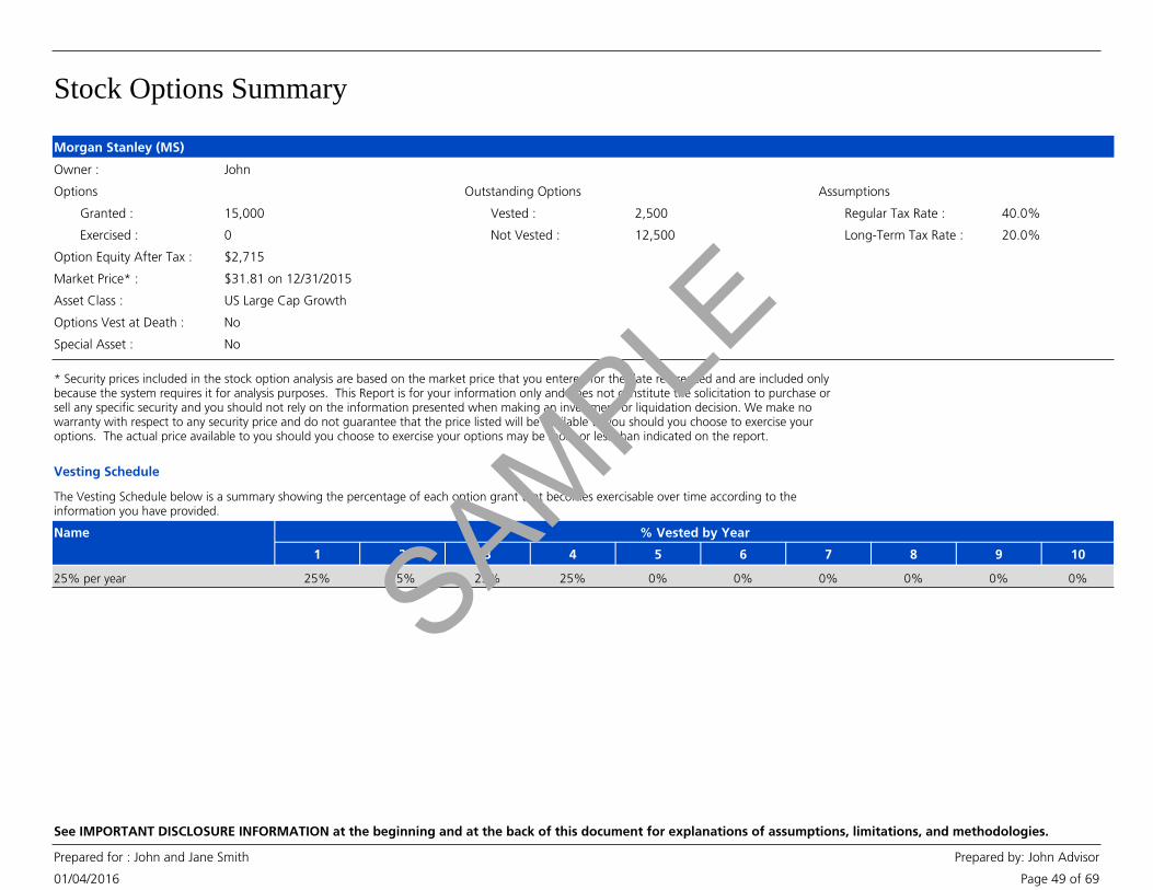
Stock Options Summary
01/04/2016
Prepared for : John and Jane Smith Prepared by: John Advisor
Page 49 of 69
See IMPORTANT DISCLOSURE INFORMATION at the beginning and at the back of this document for explanations of assumptions, limitations, and methodologies.
Morgan Stanley (MS)
Owner : John
Options
Granted :
Exercised :
Outstanding Options
Vested :
Not Vested :
15,000
0
2,500
12,500
Regular Tax Rate : 40.0%
Long-Term Tax Rate : 20.0%
Assumptions
Option Equity After Tax : $2,715
Market Price* :
Options Vest at Death :
$31.81 on 12/31/2015
No
Asset Class : US Large Cap Growth
* Security prices included in the stock option analysis are based on the market price that you entered for the date referenced and are included onlybecause the system requires it for analysis purposes. This Report is for your information only and does not constitute the solicitation to purchase orsell any specific security and you should not rely on the information presented when making an investment or liquidation decision. We make nowarranty with respect to any security price and do not guarantee that the price listed will be available to you should you choose to exercise youroptions. The actual price available to you should you choose to exercise your options may be more or less than indicated on the report.
Special Asset : No
Vesting Schedule
The Vesting Schedule below is a summary showing the percentage of each option grant that becomes exercisable over time according to theinformation you have provided.
Name % Vested by Year
1 2 3 4 5 6 7 8 9 10
25% per year 25% 25% 25% 25% 0% 0% 0% 0% 0% 0%SAMPLE
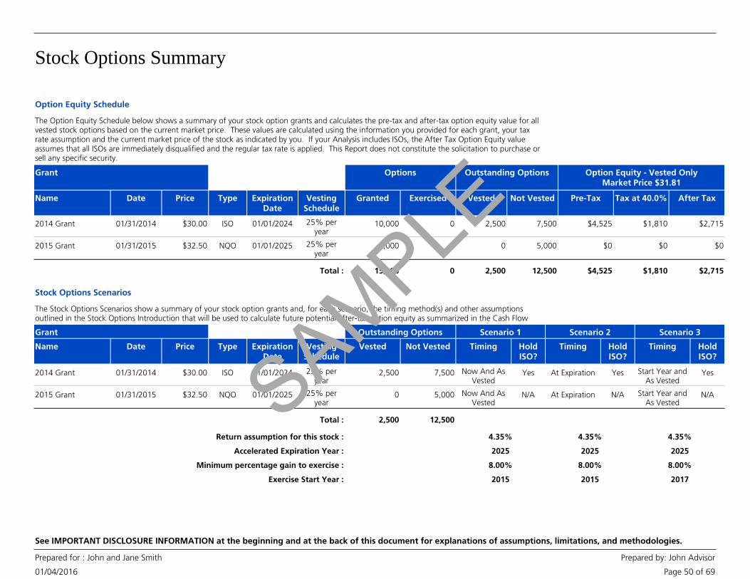
Stock Options Summary
01/04/2016
Prepared for : John and Jane Smith Prepared by: John Advisor
Page 50 of 69
See IMPORTANT DISCLOSURE INFORMATION at the beginning and at the back of this document for explanations of assumptions, limitations, and methodologies.
Option Equity Schedule
The Option Equity Schedule below shows a summary of your stock option grants and calculates the pre-tax and after-tax option equity value for allvested stock options based on the current market price. These values are calculated using the information you provided for each grant, your taxrate assumption and the current market price of the stock as indicated by you. If your Analysis includes ISOs, the After Tax Option Equity valueassumes that all ISOs are immediately disqualified and the regular tax rate is applied. This Report does not constitute the solicitation to purchase orsell any specific security.
Name Date Price Type ExpirationDate
Granted Exercised Vested Not Vested Pre-Tax Tax at 40.0%
Grant
VestingSchedule
Options Outstanding Options
After Tax
Option Equity - Vested OnlyMarket Price $31.81
2014 Grant 01/31/2014 $30.00 ISO 01/01/2024 25% peryear
10,000 0 2,500 7,500 $4,525 $1,810 $2,715
2015 Grant 01/31/2015 $32.50 NQO 01/01/2025 25% peryear
5,000 0 0 5,000 $0 $0 $0
15,000 0Total : 2,500 12,500 $4,525 $1,810 $2,715
Stock Options Scenarios
The Stock Options Scenarios show a summary of your stock option grants and, for each scenario, the timing method(s) and other assumptionsoutlined in the Stock Options Introduction that will be used to calculate future potential after-tax option equity as summarized in the Cash FlowSchedule.
Name Date Price Type ExpirationDate
Timing HoldISO?
Timing HoldISO?
Grant
VestingSchedule
Timing
Scenario 1
Vested Not Vested
Outstanding Options
HoldISO?
Scenario 2 Scenario 3
2014 Grant 01/31/2014 $30.00 ISO 01/01/2024 25% peryear
Now And AsVested
Yes At Expiration Yes Start Year andAs Vested
2,500 7,500 Yes
2015 Grant 01/31/2015 $32.50 NQO 01/01/2025 25% peryear
Now And AsVested
N/A At Expiration N/A Start Year andAs Vested
0 5,000 N/A
2,500 12,500Total :
4.35%4.35%4.35%Return assumption for this stock :
Accelerated Expiration Year : 2025 2025 2025
Minimum percentage gain to exercise : 8.00% 8.00% 8.00%
Exercise Start Year : 2015 2015 2017
SAMPLE
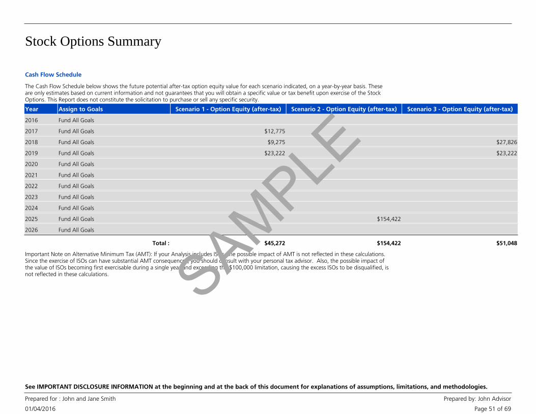
Stock Options Summary
01/04/2016
Prepared for : John and Jane Smith Prepared by: John Advisor
Page 51 of 69
See IMPORTANT DISCLOSURE INFORMATION at the beginning and at the back of this document for explanations of assumptions, limitations, and methodologies.
Cash Flow Schedule
The Cash Flow Schedule below shows the future potential after-tax option equity value for each scenario indicated, on a year-by-year basis. Theseare only estimates based on current information and not guarantees that you will obtain a specific value or tax benefit upon exercise of the StockOptions. This Report does not constitute the solicitation to purchase or sell any specific security.
Year Assign to Goals Scenario 1 - Option Equity (after-tax) Scenario 2 - Option Equity (after-tax) Scenario 3 - Option Equity (after-tax)
2016 Fund All Goals
2017 Fund All Goals $12,775
2018 Fund All Goals $27,826$9,275
2019 Fund All Goals $23,222$23,222
2020 Fund All Goals
2021 Fund All Goals
2022 Fund All Goals
2023 Fund All Goals
2024 Fund All Goals
2025 Fund All Goals $154,422
2026 Fund All Goals
$45,272 $154,422 $51,048Total :
Important Note on Alternative Minimum Tax (AMT): If your Analysis includes ISOs, the possible impact of AMT is not reflected in these calculations.Since the exercise of ISOs can have substantial AMT consequences, you should consult with your personal tax advisor. Also, the possible impact ofthe value of ISOs becoming first exercisable during a single year and exceeding the $100,000 limitation, causing the excess ISOs to be disqualified, isnot reflected in these calculations. SAMPLE

Appendix
SAMPLE

Risk Assessment
01/04/2016
Prepared for : John and Jane Smith Prepared by: John Advisor
Page 52 of 69
See IMPORTANT DISCLOSURE INFORMATION at the beginning and at the back of this document for explanations of assumptions, limitations, and methodologies.
Investment Account
Other
Current Income
Educational Planning
Major Purchase
Retirement
Yes
No
Less than 2%
Greater than 2%, but less than 4%
Greater than 4%, but less than 6%
Greater than 6%
Over 20 years
11 - 20 years
6 - 10 years
1 - 5 years
Immediately
I am primarily concerned with maximizing the returns of my investments. I amwilling to accept high risk and high chance of loss to maximize my investment returnpotential.
I am willing to accept moderate risk and chance of loss in order to achieve moderatereturns. Limiting risk and maximizing return are of equal importance to me.
I am most concerned with limiting risk. I am willing to accept lower expectedreturns in order to limit my chance of loss.
1. What is your primary purpose for investing in this account?
2. Do you need current income (that is, will you take regular withdrawals from thisaccount)?
If yes, approximately what percentage of the accounts current value do you needannually?
3. In approximately how many years will you begin withdrawing funds for yourinvestment objective?
Over 20 years
11 - 20 years
6 - 10 years
1 - 5 years
Lump Sum
4. Once you begin to withdraw funds for your primary investment objective, over howlong a period do you anticipate the withdrawals to continue?
5. Which of the following statements best describes your attitude towards the trade-offbetween risk and return?
Updated : 09/03/2015
SAMPLE
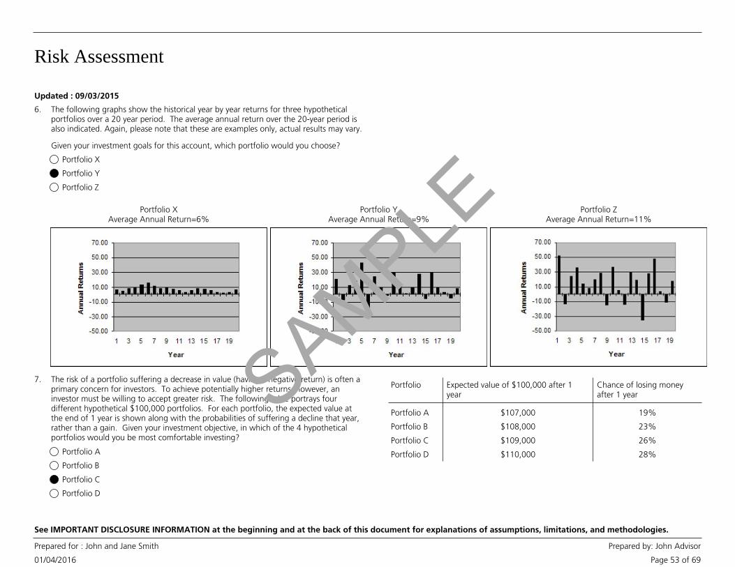
Risk Assessment
01/04/2016
Prepared for : John and Jane Smith Prepared by: John Advisor
Page 53 of 69
See IMPORTANT DISCLOSURE INFORMATION at the beginning and at the back of this document for explanations of assumptions, limitations, and methodologies.
Updated : 09/03/2015
Portfolio X
Portfolio Y
Portfolio Z
6. The following graphs show the historical year by year returns for three hypotheticalportfolios over a 20 year period. The average annual return over the 20-year period isalso indicated. Again, please note that these are examples only, actual results may vary.
Given your investment goals for this account, which portfolio would you choose?
Portfolio XAverage Annual Return=6%
Portfolio YAverage Annual Return=9%
Portfolio ZAverage Annual Return=11%
7. The risk of a portfolio suffering a decrease in value (having a negative return) is often aprimary concern for investors. To achieve potentially higher returns, however, aninvestor must be willing to accept greater risk. The following table portrays fourdifferent hypothetical $100,000 portfolios. For each portfolio, the expected value atthe end of 1 year is shown along with the probabilities of suffering a decline that year,rather than a gain. Given your investment objective, in which of the 4 hypotheticalportfolios would you be most comfortable investing?
Portfolio A
Portfolio B
Portfolio C
Portfolio D
Portfolio Expected value of $100,000 after 1year
Portfolio A
Portfolio B
Portfolio C
Portfolio D
Chance of losing moneyafter 1 year
$107,000
$108,000
$109,000
$110,000
19%
23%
26%
28%
SAMPLE
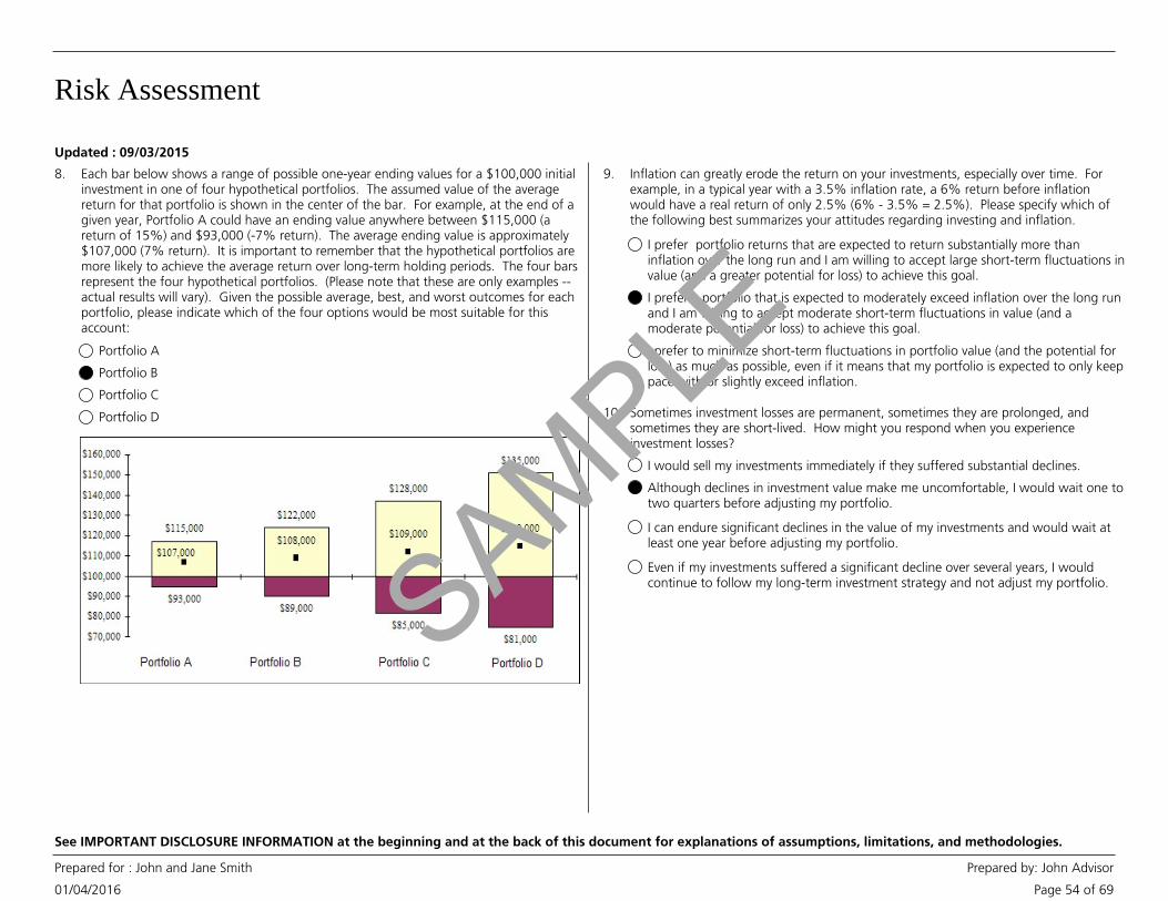
Risk Assessment
01/04/2016
Prepared for : John and Jane Smith Prepared by: John Advisor
Page 54 of 69
See IMPORTANT DISCLOSURE INFORMATION at the beginning and at the back of this document for explanations of assumptions, limitations, and methodologies.
Updated : 09/03/2015
8. Each bar below shows a range of possible one-year ending values for a $100,000 initialinvestment in one of four hypothetical portfolios. The assumed value of the averagereturn for that portfolio is shown in the center of the bar. For example, at the end of agiven year, Portfolio A could have an ending value anywhere between $115,000 (areturn of 15%) and $93,000 (-7% return). The average ending value is approximately$107,000 (7% return). It is important to remember that the hypothetical portfolios aremore likely to achieve the average return over long-term holding periods. The four barsrepresent the four hypothetical portfolios. (Please note that these are only examples --actual results will vary). Given the possible average, best, and worst outcomes for eachportfolio, please indicate which of the four options would be most suitable for thisaccount:
Portfolio A
Portfolio B
Portfolio C
Portfolio D
9. Inflation can greatly erode the return on your investments, especially over time. Forexample, in a typical year with a 3.5% inflation rate, a 6% return before inflationwould have a real return of only 2.5% (6% - 3.5% = 2.5%). Please specify which ofthe following best summarizes your attitudes regarding investing and inflation.
I prefer portfolio returns that are expected to return substantially more thaninflation over the long run and I am willing to accept large short-term fluctuations invalue (and a greater potential for loss) to achieve this goal.
I prefer a portfolio that is expected to moderately exceed inflation over the long runand I am willing to accept moderate short-term fluctuations in value (and amoderate potential for loss) to achieve this goal.
I prefer to minimize short-term fluctuations in portfolio value (and the potential forloss) as much as possible, even if it means that my portfolio is expected to only keeppace with or slightly exceed inflation.
10. Sometimes investment losses are permanent, sometimes they are prolonged, andsometimes they are short-lived. How might you respond when you experienceinvestment losses?
I would sell my investments immediately if they suffered substantial declines.
Although declines in investment value make me uncomfortable, I would wait one totwo quarters before adjusting my portfolio.
I can endure significant declines in the value of my investments and would wait atleast one year before adjusting my portfolio.
Even if my investments suffered a significant decline over several years, I wouldcontinue to follow my long-term investment strategy and not adjust my portfolio.SAMPLE
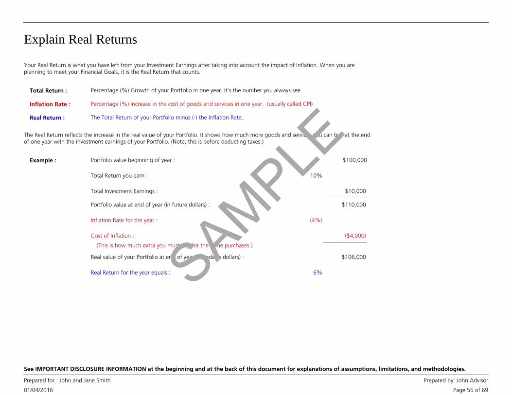
Explain Real Returns
01/04/2016
Prepared for : John and Jane Smith Prepared by: John Advisor
Page 55 of 69
See IMPORTANT DISCLOSURE INFORMATION at the beginning and at the back of this document for explanations of assumptions, limitations, and methodologies.
Your Real Return is what you have left from your Investment Earnings after taking into account the impact of Inflation. When you areplanning to meet your Financial Goals, it is the Real Return that counts.
Total Return :
Inflation Rate :
Real Return :
Percentage (%) Growth of your Portfolio in one year. It's the number you always see.
Percentage (%) increase in the cost of goods and services in one year. (usually called CPI)
The Total Return of your Portfolio minus (-) the Inflation Rate.
The Real Return reflects the increase in the real value of your Portfolio. It shows how much more goods and services you can buy at the endof one year with the investment earnings of your Portfolio. (Note, this is before deducting taxes.)
Example : Portfolio value beginning of year :
Total Return you earn :
Total Investment Earnings :
Portfolio value at end of year (in future dollars) :
Inflation Rate for the year :
Cost of Inflation :
(This is how much extra you must pay for the same purchases.)
Real value of your Portfolio at end of year (in today's dollars) :
Real Return for the year equals :
$100,000
10%
$10,000
$110,000
(4%)
($4,000)
$106,000
6%SAMPLE
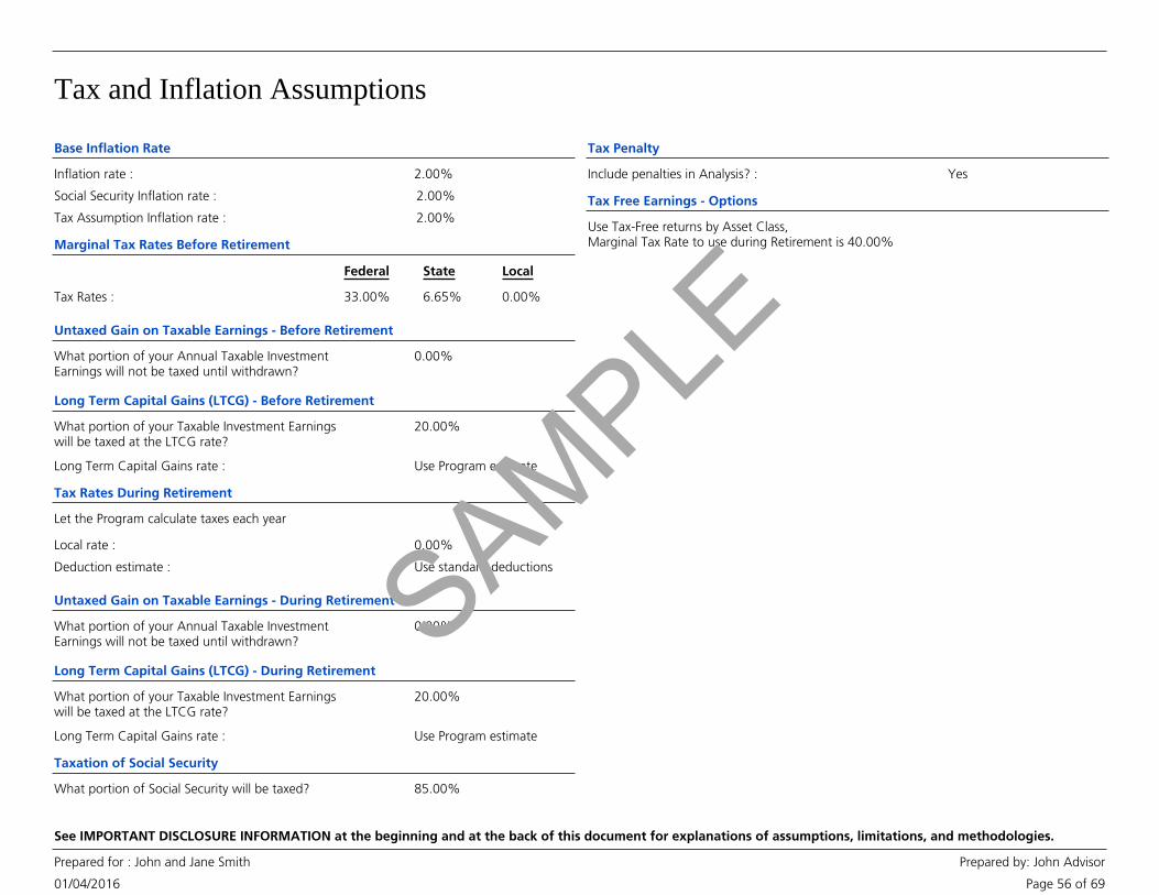
Tax and Inflation Assumptions
01/04/2016
Prepared for : John and Jane Smith Prepared by: John Advisor
Page 56 of 69
See IMPORTANT DISCLOSURE INFORMATION at the beginning and at the back of this document for explanations of assumptions, limitations, and methodologies.
Base Inflation Rate
Inflation rate : 2.00%
Social Security Inflation rate : 2.00%
Tax Assumption Inflation rate : 2.00%
Tax Rates : 33.00%
Federal
6.65%
State
0.00%
Local
Marginal Tax Rates Before Retirement
Untaxed Gain on Taxable Earnings - Before Retirement
What portion of your Annual Taxable InvestmentEarnings will not be taxed until withdrawn?
0.00%
What portion of your Taxable Investment Earningswill be taxed at the LTCG rate?
20.00%
Long Term Capital Gains rate : Use Program estimate
Long Term Capital Gains (LTCG) - Before Retirement
Tax Rates During Retirement
Local rate : 0.00%
Deduction estimate : Use standard deductions
Let the Program calculate taxes each year
0.00%
Untaxed Gain on Taxable Earnings - During Retirement
What portion of your Annual Taxable InvestmentEarnings will not be taxed until withdrawn?
Long Term Capital Gains (LTCG) - During Retirement
What portion of your Taxable Investment Earningswill be taxed at the LTCG rate?
20.00%
Long Term Capital Gains rate : Use Program estimate
Taxation of Social Security
What portion of Social Security will be taxed? 85.00%
Tax Penalty
Include penalties in Analysis? : Yes
Use Tax-Free returns by Asset Class,Marginal Tax Rate to use during Retirement is 40.00%
Tax Free Earnings - Options
SAMPLE
IMPORTANT DISCLOSURE INFORMATION
01/04/2016
Prepared for : John and Jane Smith Prepared by: John Advisor
Page 57 of 69
Report Is a Snapshot and Does Not Provide Legal, Tax, or Accounting Advice
This Report provides a snapshot of your current financial position and can help you to focuson your financial resources and goals, and to create a plan of action. Because the resultsare calculated over many years, small changes can create large differences in future results.You should use this Report to help you focus on the factors that are most important to you.This Report does not provide legal, tax, or accounting advice. Before making decisions withlegal, tax, or accounting ramifications, you should consult appropriate professionals foradvice that is specific to your situation.
A Note on Tax-Qualified/Tax-Deferred Assets
If your portfolio contains assets which are tax-qualified or tax-deferred under the InternalRevenue Code, you should consider the tax effects of any portfolio withdrawal from suchamounts, as opposed to from fully taxable accounts, with your tax and/or legal advisor(s).Generally speaking, the withdrawal of tax-qualified or tax-deferred amounts can result inincome tax liability where no such liability would exist if the amounts had been withdrawnfrom a taxable account. Furthermore, (a) tax penalties can occur when such assets arewithdrawn prior to age 59½, (b) such withdrawals can have detrimental effects on specifictax planning strategies (e.g., “72(t) payments”), and (c) certain qualified or tax-deferredassets are eligible for or receive special treatment upon withdrawal (e.g., net unrealizedappreciation treatment, eligibility for rollover). In light of the foregoing, we stronglyrecommend that you consult your tax and/or legal advisors in connection with this Reportand any withdrawals that you make from your portfolio.
What If Worksheets allow you to review and compare the results of your LifeView GoalAnalysis. The Worksheets provide you with tools to consider alternative solutions.
What If Scenarios
LifeView Goal Analysis Methodology
LifeView Goal Analysis offers several methods of calculating results, each of which providesone outcome from a wide range of possible outcomes. The methods used are: “AverageReturns,” “Bad Timing,” “Class Sensitivity,” and “Monte Carlo Simulations.”
Results Using Average Returns
The Results Using Average Returns are calculated using one average return for yourpre-retirement period and one average return for your post-retirement period. AverageReturns are a simplifying assumption. In reality, investment returns can (and often do) varywidely from year to year and vary widely from a long-term average return.
Results with Bad Timing
Results with Bad Timing are calculated by using low returns in one or two years, andaverage returns for all remaining years of the Analysis. For most Analyses, the worst timefor low returns is when you begin taking substantial withdrawals from your portfolio. TheResults with Bad Timing assume that you earn a low return in the year(s) you select andthen an Adjusted Average Return in all other years. This Adjusted Average Return iscalculated so that the average return of the Results with Bad Timing is equal to the return(s)used in calculating the Results Using Average Returns. This allows you to compare tworesults with the same overall average return, where one (the Results with Bad Timing) haslow returns in one or two years.
The default for the first year of low returns is two standard deviations less than the averagereturn, and the default for the second year is one standard deviation less than the averagereturn.
The Results Using Class Sensitivity are calculated by using different return assumptions forone or more asset classes during the years you select. These results show how your Analysiswould be affected if the annual returns for one or more asset classes were different thanthe average returns for a specified period in your Analysis.
Results Using Class Sensitivity
LifeView Goal Analysis Presentation of Results
The Results Using Average Returns, Bad Timing, and Class Sensitivity display the resultsusing an “Estimated % of Goal Funded” and a “Safety Margin.”
Estimated % of Goal Funded
For each Goal, the “Estimated % of Goal Funded” is the sum of the assets used to fund theGoal divided by the sum of the Goal’s expenses. All values are in current dollars. A result of100% or more does not guarantee that you will reach a Goal, nor does a result under100% guarantee that you will not. Rather, this information is meant to identify possibleshortfalls in this Analysis, and is not a guarantee that a certain percentage of your Goals willbe funded. The percentage reflects a projection of the total cost of the Goal that wasactually funded based upon all the assumptions that are included in this Analysis, andassumes that you execute all aspects of the Analysis as you have indicated.
The Safety Margin is the estimated value of your assets at the end of this Analysis, based onall the assumptions included in this Report. Only you can determine if that Safety Margin issufficient for your needs.
Safety Margin
SAMPLE

IMPORTANT DISCLOSURE INFORMATION
01/04/2016
Prepared for : John and Jane Smith Prepared by: John Advisor
Page 58 of 69
Bear Market Loss and Bear Market Test
The Bear Market Loss shows how a portfolio would have been impacted during the worstbear market since the Great Depression. Depending on the composition of the portfolio,the worst bear market is either the "Great Recession" or the "Bond Bear Market."
The Great Recession, from November 2007 through February 2009, was the worst bearmarket for stocks since the Great Depression. In LifeView Goal Analysis, the Great RecessionReturn is the rate of return, during the Great Recession, for a portfolio comprised of cash,bonds, stocks, and alternatives, with an asset mix equivalent to the portfolio referenced.
The Bond Bear Market, from July 1979 through February 1980, was the worst bear marketfor bonds since the Great Depression. In LifeView Goal Analysis, the Bond Bear MarketReturn is the rate of return, for the Bond Bear Market period, for a portfolio comprised ofcash, bonds, stocks, and alternatives, with an asset mix equivalent to the portfolioreferenced.
The Bear Market Loss shows: 1) either the Great Recession Return or the Bond Bear MarketReturn, whichever is lower, and 2) the potential loss, if you had been invested in thiscash-bond-stock-alternative portfolio during the period with the lower return. In general,most portfolios with a stock allocation of 20% or more have a lower Great RecessionReturn, and most portfolios with a combined cash and bond allocation of 80% or morehave a lower Bond Bear Market Return.
The Bear Market Test, included in the Stress Tests, examines the impact on your Analysisresults if an identical Great Recession or Bond Bear Market, whichever would be worse,occurred this year. The Bear Market Test shows the likelihood that you could fund yourNeeds, Wants and Wishes after experiencing such an event.
Regardless of whether you are using historical or projected returns for all other LifeViewGoal Analysis results, the Bear Market Loss and Bear Market Test use returns calculatedfrom historical indices. If you are using historical returns, the indices in the Bear Market Lossand the Bear Market Test may be different from indices used in other calculations. Theseresults are calculated using only four asset classes – Cash, Bonds, Stocks, and Alternatives.The indices and the resulting returns for the Great Recession and the Bond Bear Market are:
Asset Class Index Great RecessionReturn
11/2007 – 02/2009
Bond Bear MarketReturn
07/1979 – 02/1980
Cash Ibbotson U.S. 30-dayTreasury Bills
2.31% 7.08%
Bond Ibbotson Intermediate-TermGovernment Bonds – TotalReturn
15.61% -8.89%
Stock S&P 500 - Total Return -50.95% 14.61%
Alternative HFRI FOF: Diversified*S&P GSCI Commodity - TotalReturn**
-19.87%N/A
N/A23.21%
*Hedge Fund Research Indices Fund of Funds
**S&P GSCI was formerly the Goldman Sachs Commodity Index
Because the Bear Market Loss and Bear Market Test use the returns from asset class indicesrather than the returns of actual investments, they do not represent the performance forany specific portfolio, and are not a guarantee of minimum or maximum levels of losses orgains for any portfolio. The actual performance of your portfolio may differ substantiallyfrom those shown in the Great Recession Return, the Bond Bear Market Return, the BearMarket Loss, and the Bear Market Test.
SAMPLE
Return Methodology and Asset Allocation
01/04/2016
Prepared for : John and Jane Smith Prepared by: John Advisor
Page 59 of 69
“Rebalancing” describes the discipline of selling assets and buying others to match the target weightings of an asset allocation model.Because assets increase and decrease in value over time, the percentage amounts of assets invested in each class will tend to vary from theiroriginal target weightings.
Morgan Stanley Wealth Management Global Investment Committee Secular ReturnEstimates Methodology
This tool incorporates a methodology for making hypothetical financial projections approvedby the Morgan Stanley Wealth Management Global Investment Committee. Opinionsexpressed in this presentation may differ materially from those expressed by otherdepartments or divisions or affiliates of Morgan Stanley.
About Secular Return Estimates, Rate of Return, Standard Deviation, and AssetClass Indices
Secular Return Estimates (SREs)
What are SREs?
These Secular Return Estimates (SREs) represent one set of assumptions regarding rates ofreturn for specific asset classes approved by the Morgan Stanley Wealth ManagementGlobal Investment Committee. However, this tool allows you to modify the SREs in what-ifscenarios and/or stress testing to include your own assumptions about the rates of returnyou may expect to receive on various asset classes. Changing these assumptions can changethe program results.
How are SREs derived?
These assumptions are made using a proprietary methodology using a building blockapproach. Our SREs reflect expectations for a number of long-term economic andmarket-related factors we expect to influence capital market returns, such as populationgrowth, productivity, long-term average dividend payout and net repurchase rates, etc.
Index returns are used for calculation of volatility and correlations. For most indices we usedata since 1994. Regarding several types of alternative investments such as hedge funds,private equity and real estate, we apply significant statistical adjustments to historicalreturns in order to correct for distortions such as survivorship biases, selection biases andprice staleness.
What else is important to know?
It is important to remember that future rates of return can't be predicted with certainty andthat investments that may provide higher rates of return are generally subject to higher riskand volatility. The actual rate of return on investments can vary widely over time. Thisincludes the potential loss of principal on your investment.
1
Investors should carefully consider several important factors when making asset allocationdecisions using projected investment performance data based on assumed rates of return ofindices:
Indices illustrate the investment performance of instruments that have certain similarcharacteristics and are intended to reflect broad segments of an asset class. Indices do notrepresent the actual or hypothetical performance of any specific investment, including anyindividual security within an index. Although some indices can be replicated, it is notpossible to directly invest in an index. It is important to remember the investmentperformance of an index does not reflect deductions for investment charges, expenses, orfees that may apply when investing in securities and financial instruments such ascommissions, sales loads, or other applicable fees. Also, the stated investment performanceassumes the reinvestment of interest and dividends at net asset value without taxes, andalso assumes that the portfolio is consistently “rebalanced” to the initial target weightings.Asset allocations which deviate significantly from the initial weightings can significantlyaffect the likelihood of achieving the projected investment performance.
1
Another important factor to keep in mind when considering the historical and projectedreturns of indices is that the risk of loss in value of a specific asset, such as a stock, a bondor a share of a mutual fund, is not the same as, and does not match, the risk of loss in abroad asset class index. As a result, the investment performance of an index will not be thesame as the investment performance of a specific instrument, including one that iscontained in the index. Such a possible lack of “investment performance correlation” mayalso apply to the future of a specific instrument relative to an index.
For these reasons, the ultimate decision to invest in specific instruments should not bepremised on expectations that the historical or projected returns of indices will be the sameas those for specific investments made.
These assumptions are subject to change. Please note that some time may be required toimplement any changes into the tool. SAMPLE
Return Methodology and Asset Allocation
01/04/2016
Prepared for : John and Jane Smith Prepared by: John Advisor
Page 60 of 69
Morgan Stanley Wealth Management Global Investment Committee Secular ReturnEstimates Methodology (continued)
It is important to note that the rates of return of the listed indices may be significantlydifferent than the SRE or your own assumptions about the rates of return used in thereport. As always, keep in mind that past performance is no guarantee of future results.SREs are for illustrative purposes only and are not indicative of the future performance ofany specific investment.
Performance of an asset class within a portfolio is dependent upon the allocation ofsecurities within the asset class and the weighting or the percentage of the asset classwithin that portfolio. Potential for a portfolio’s loss is exacerbated in a downward trendingmarket. A well-diversified portfolio is less vulnerable in a falling market. Asset allocation anddiversification, however, do not assure a profit or protect against loss in a declining market.
Asset class returns and standard deviations of returns projections are based on reasonedestimates of drivers of capital market returns and historical relationships. As with anyforecasting discipline, the assumptions and inputs underlying Morgan Stanley WealthManagement’s forecasting process may or may not reconcile with, or reflect, each investor’sindividual investment horizon, risk tolerance, capital markets outlook, and world view. Forthese reasons, and because forecasting methods are complicated, investors are encouragedto discuss forecasting with a Morgan Stanley Financial Advisor.
While Morgan Stanley Wealth Management has not designed its forecasting methodologiesto match or address its inventory as a broker-dealer of financial products, the MorganStanley Wealth Management forecasts, if followed, guide investors in directions thatsupport Morgan Stanley Wealth Management's inventory.
Asset Allocation
Asset Allocation refers to how your investments are diversified across different asset classes,such as Stocks, Bonds, Cash and Alternative Investments. The principal asset classes andcomparative indices for each asset class presented in this analysis can be found in the ReturnMethodology chart. The Target Portfolio falls within the limits of your risk tolerance, basedon your answers to the risk assessment (risk profile questionnaire). Either a Morgan StanleyWealth Management Global Investment Committee (GIC) Strategic Asset Allocation Modelor a customized asset allocation is presented. The asset allocation you selected may be moreconservative than your investment risk profile. This approach may change the programresults. Morgan Stanley Global Investment Committee uses a proprietary process to arrive atits strategic asset allocation models. These models are subject to change and some time maybe required to implement any such changes into the tool.
Rates of Return, Standard Deviation, and Asset Class Indices
Standard deviation is a common risk measurement that estimates how much aninvestment’s return will vary from its predicted average. Generally, the higher aninvestment’s standard deviation, the more widely its returns will fluctuate, implying greatervolatility. In the past, asset classes that have typically provided the highest returns have alsocarried greater risk. For purposes of this report, the standard deviation for the asset classesshown below are calculated using data going back 20 years.
SAMPLE
Return Methodology and Asset Allocation
01/04/2016
Prepared for : John and Jane Smith Prepared by: John Advisor
Page 61 of 69
Return IndexAsset Class
Cash
Cash - Strategic Citi T-Bills 90-Day
Stock
US Large Cap Growth Russell 1000 Growth
US Large Cap Value Russell 1000 Value
US Mid Cap Growth Russell MidCap Growth
US Mid Cap Value Russell MidCap Value
US Small Cap Growth Russell 2000 Growth
US Small Cap Value Russell 2000 Value
US Equity Other S&P 500
International Equity MSCI World ex US Net
Emerging Markets Equity MSCI Emerging Markets Net
Global Equity Other MSCI All Country World Index Net
Bond
Ultra Short Fixed Income Citi T-Bills 90-Day
Short Term Fixed Income Barclays Global Aggregate(1-3yr)
US Fixed Income Barclays Capital US Aggregate
International Fixed Income Barclays Capital Global Aggregate Non-USD
Inflation-linked Securities Barclays Capital Global Inflation-Linked Index
High Yield Fixed Income Barclays Capital Global High Yield
Emerging Markets Fixed Income JP Morgan Emerging Market Bond Index Global Total Return
Global Fixed Income Other Barclays Capital Global AggregateSAMPLE
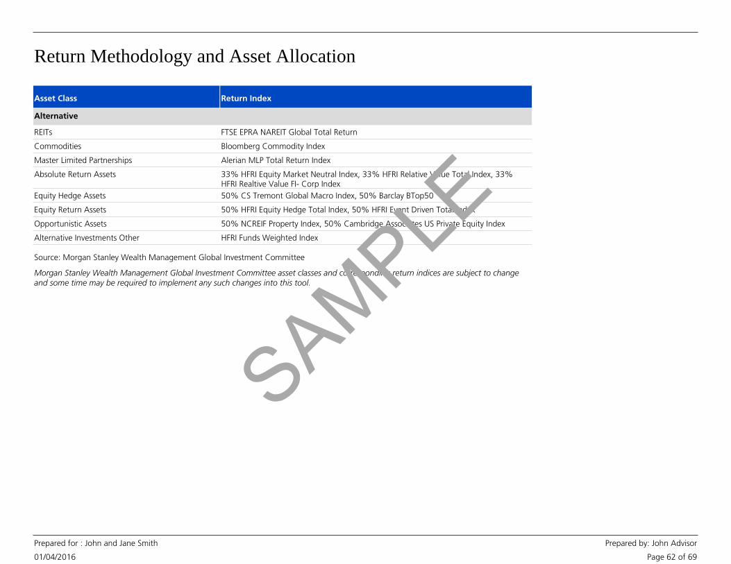
Return Methodology and Asset Allocation
01/04/2016
Prepared for : John and Jane Smith Prepared by: John Advisor
Page 62 of 69
Return IndexAsset Class
Alternative
REITs FTSE EPRA NAREIT Global Total Return
Commodities Bloomberg Commodity Index
Master Limited Partnerships Alerian MLP Total Return Index
Absolute Return Assets 33% HFRI Equity Market Neutral Index, 33% HFRI Relative Value Total Index, 33%HFRI Realtive Value FI- Corp Index
Equity Hedge Assets 50% CS Tremont Global Macro Index, 50% Barclay BTop50
Equity Return Assets 50% HFRI Equity Hedge Total Index, 50% HFRI Event Driven Total Index
Opportunistic Assets 50% NCREIF Property Index, 50% Cambridge Associates US Private Equity Index
Alternative Investments Other HFRI Funds Weighted Index
Source: Morgan Stanley Wealth Management Global Investment Committee
Morgan Stanley Wealth Management Global Investment Committee asset classes and corresponding return indices are subject to changeand some time may be required to implement any such changes into this tool.
SAMPLE

Key Asset Class Risk Considerations
01/04/2016
Prepared for : John and Jane Smith Prepared by: John Advisor
Page 63 of 69
Alternative Investments
The asset allocation recommendations provided to you in this report may include allocationsto alternative asset classes. It is important to note that Alternatives may be either traditionalalternative investment vehicles or non-traditional alternative strategy products. Traditionalalternative investment vehicles may include hedge funds, fund of hedge funds (bothregistered and unregistered), private equity, and private real estate or managed futuresfunds. Non-traditional alternative strategy products may include open-end mutual funds andETFs. These non-traditional products also seek alternative-like exposure but have significantdifferences from traditional alternative investments.
The risks of traditional alternative investments may include: can be highly illiquid, speculativeand not suitable for all investors, loss of all or a substantial portion of the investment due toleveraging, short-selling, or other speculative practices, volatility of returns, restrictions ontransferring interests in a fund, potential lack of diversification and resulting higher risk dueto concentration of trading authority when a single advisor is utilized, absence ofinformation regarding valuations and pricing, complex tax structures and delays in taxreporting, less regulation and higher fees than open-end mutual funds, and risks associatedwith the operations, personnel and processes of the manager. Non-traditional alternativestrategy products may employ various investment strategies and techniques for bothhedging and more speculative purposes such as short-selling, leverage, derivatives andoptions, which can increase volatility and the risk of investment loss.
REITs
In addition to the general risks associated with real estate investments, REIT investing entailsother risks such as credit and interest rate risk. Real estate investment risks can includefluctuations in the value of underlying properties; defaults by borrowers or tenants; marketsaturation; changes in general and local economic conditions; decreases in market rates forrents; increases in competition, property taxes, capital expenditures, or operating expenses;and other economic, political or regulatory occurrences affecting the real estate industry.
Commodities
The commodities markets may fluctuate widely based on a variety of factors includingchanges in supply and demand relationships; governmental programs and policies; nationaland international political and economic events; war and terrorist events; changes in interestand exchange rates; trading activities in commodities and related contracts; pestilence;weather; technological change; and, the price volatility of a commodity. In addition, thecommodities markets are subject to temporary distortions or other disruptions due tovarious factors, including lack of liquidity, participation of speculators and governmentintervention.
Master Limited Partnerships (MLPs) are limited partnerships or limited liability companiesthat are taxed as partnerships and whose interests (limited partnership units or limitedliability company units) are traded on securities exchanges like shares of common stock.Currently, most MLPs operate in the energy, natural resources or real estate sectors.Investments in MLP interests are subject to the risks generally applicable to companies in theenergy and natural resources sectors, including commodity pricing risk, supply and demandrisk, depletion risk and exploration risk.
Master Limited Partnerships (MLPs)
Individual MLPs are publicly traded partnerships that have unique risks related to theirstructure. These include, but are not limited to, their reliance on the capital markets to fundgrowth, adverse ruling on the current tax treatment of distributions (typically mostly taxdeferred), and commodity volume risk.
The potential tax benefits from investing in MLPs depend on their being treated aspartnerships for federal income tax purposes and, if the MLP is deemed to be a corporation,then its income would be subject to federal taxation at the entity level, reducing the amountof cash available for distribution to the fund which could result in a reduction of the fund’svalue.
MLPs carry interest rate risk and may underperform in a rising interest rate environment.MLP funds accrue deferred income taxes for future tax liabilities associated with the portionof MLP distributions considered to be a tax-deferred return of capital and for any netoperating gains as well as capital appreciation of its investments; this deferred tax liability isreflected in the daily NAV; and, as a result, the MLP fund’s after-tax performance coulddiffer significantly from the underlying assets even if the pre-tax performance is closelytracked.
Fixed Income
Investing in fixed income securities involves interest rate risk, credit risk, and inflation risk.Interest rate risk is the possibility that bond prices will decrease because of an interest rateincrease. When interest rates rise, bond prices, and the values of fixed income securitiesgenerally fall. Credit risk is the risk that a company will not be able to pay its debts,including the interest on its bonds. Inflation risk is the possibility that the interest paid on aninvestment in bonds will be lower than the inflation rate, decreasing purchasing power.
SAMPLE

Key Asset Class Risk Considerations
01/04/2016
Prepared for : John and Jane Smith Prepared by: John Advisor
Page 64 of 69
Ultra-Short Fixed Income
Ultra-short bond funds are mutual funds and exchange-traded funds that generally invest infixed income securities with very short maturities, typically less than one year. They are notmoney market funds. While money market funds attempt to maintain a stable net assetvalue, an ultra-short bond fund’s net asset value will fluctuate, which may result in the lossof the principal amount invested. They are therefore subject to the risks associated withdebt securities such as credit and interest rate risk.
Non-US Fixed Income
Foreign fixed income securities may involve greater risks than those issued by U.S.companies or the U.S. government. Economic, political and other events unique to acountry or region will affect those markets and their issues, but may not affect the U.S.market or similar U.S. issuers.
Inflation-Linked Securities
These securities adjust periodically against a benchmark rate, such as the Consumer PriceIndex (CPI). They pay a coupon equal to the benchmark rate, plus a fixed 'spread' and reseton a periodic basis. The initial interest rate on an inflation linked or floating security may belower than that of a fixed-rate security of the same maturity because investors expect toreceive additional income due to future increases in CPI, or the linked reference interestrate. However, there can be no assurance that these increases will occur.
High Yield Fixed Income
High yield fixed income securities, also known as “junk bonds”, are considered speculative,involve greater risk of default and tend to be more volatile than investment grade fixedincome securities.
Municipal Fixed Income
Income generated from an investment in a municipal bond is generally exempt from federalincome taxes. Some income may be subject to state and local taxes and to the federalalternative minimum tax. Capital gains, if any, are subject to tax.
Stocks
Investing in stock securities involves volatility risk, market risk, business risk, and industryrisk. The prices of stocks fluctuate. Volatility risk is the chance that the value of a stock willfall. Market risk is the chance that the prices of all stocks will fall due to conditions in theeconomic environment. Business risk is the chance that a specific company’s stock will fallbecause of issues affecting it such as the way the company is managed. Industry risk is thechance that a set of factors particular to an industry group will adversely affect stock priceswithin the industry. (See “Asset Class – Stocks” in the Glossary section at the back of thisreport for a summary of the relative potential volatility of different types of stocks.)
Small/Mid Cap Equity
Stocks of small and medium-sized companies entail special risks, such as limited productlines, markets, and financial resources, and greater market volatility than securities of larger,more established companies.
International/Emerging Markets Equities
Foreign investing involves certain risks not typically associated with investments in domesticcorporations and obligations issued by the U.S. government, such as currency fluctuationsand controls, restrictions on foreign investments, less governmental supervision andregulation, less liquidity and the potential for market volatility and political instability. Inaddition, the securities markets of many of the emerging markets are substantially smaller,less developed, less liquid and more volatile than the securities of the U.S. and other moredeveloped countries.
SAMPLE

Glossary of Terms
01/04/2016
Prepared for : John and Jane Smith Prepared by: John Advisor
Page 65 of 69
Absolute Return
An absolute return strategy seeks positive returns unaffected by market directions.
Adjusted Real Return
Adjusted Real Return is the Real Return minus the Total Return Adjustment.
Aspirational Bucket Strategy
This optional strategy simulates segmenting a portion of your investments from those usedto cover your identified goals, and investing these assets differently than your TargetPortfolio. The analysis calculates a range of potential outcomes for the portfolio based onthe growth assumptions assigned to this segment. Generally, this strategy is used toillustrate an alternate investment strategy for funds remaining after fulfilling your financialgoals, or to model the potential growth of investments that have been earmarked for alegacy goal.
Asset Allocation is the process of determining what portions of your portfolio holdings areto be invested in the various asset classes.
Asset Allocation
Asset Class is a standard term that broadly defines a category of investments. The four basicasset classes are Cash, Bonds, Stocks and Alternatives. Bonds and Stocks are often furthersubdivided into more narrowly defined classes. Some of the most common asset classes aredefined below.
Asset Class
Cash
Cash and Cash Alternatives are investments of high liquidity and safety with a knownmarket value and a very short-term maturity. Examples are money market funds.
Bonds
Bonds are either domestic (U.S.) or global debt securities issued by either privatecorporations or governments. (See “Fixed Income" in the "Key Asset Class RiskConsiderations" section of this report for a summary of the risks associated with investingin bonds. Bonds are also called “fixed income securities.”)
Domestic stocks are equity securities of U.S. corporations. Domestic stocks are oftensub-divided based upon the market capitalization of the company (the market value of thecompany's stock). "Large cap" stocks are from larger companies, "mid cap" from themiddle range of companies, and "small cap" from smaller, perhaps newer, companies.Generally, small cap stocks experience greater market volatility than stocks of companieswith larger capitalization. Small cap stocks are generally those from companies whosecapitalization is less than $500 million, mid cap stocks those between $500 million and $5billion, and large cap over $5 billion.
Large cap, mid cap and small cap may be further sub-divided into "growth" and "value"categories. Growth companies are those with an orientation towards growth, oftencharacterized by commonly used metrics such as higher price-to-book andprice-to-earnings ratios. Analogously, value companies are those with an orientationtowards value, often characterized by commonly used metrics such as lower price-to-bookand price-to-earnings ratios.
International stocks are equity securities from foreign corporations. International stocks areoften sub-divided into those from "developed" countries and those from "emergingmarkets." The emerging markets are in less developed countries with emerging economiesthat may be characterized by lower income per capita, less developed infrastructure andnascent capital markets. These "emerging markets" usually are less economically andpolitically stable than the "developed markets." Investing in international stocks involvesspecial risks, among which include foreign exchange volatility and risks of investing underdifferent tax, regulatory and accounting standards.
Alternatives
See "Alternatives" in Key Asset Class Risk considerations.
Stocks
Stocks are equity securities of domestic and foreign corporations. (See "Stocks" in the"Key Asset Class Risk Considerations" section of this report for a summary of the risksassociated with investing in stocks.)
Domestic government bonds are backed by the full faith and credit of the U.S.Government and have superior liquidity and, when held to maturity, safety of principal.Domestic corporate bonds carry the credit risk of their issuers and thus usually offeradditional yield. Domestic government and corporate bonds can be sub-divided basedupon their term to maturity.
Ultra-short term bonds have a maturity less than 1 year; short-term bonds have anapproximate term to maturity of 1 to 5 years; intermediate-term bonds have anapproximate term to maturity of 5 to 10 years; and, long-term bonds have an approximateterm to maturity greater than 10 years.
SAMPLE

Glossary of Terms
01/04/2016
Prepared for : John and Jane Smith Prepared by: John Advisor
Page 66 of 69
Asset Mix
Asset Mix is the combination of asset classes within a portfolio, and is usually expressed as apercentage for each asset class.
Bear Market Loss
The Bear Market Loss shows how a portfolio would have been impacted during the GreatRecession (November 2007 through February 2009) or the Bond Bear Market (July 1979through February 1980). The Bear Market Loss shows: 1) either the Great Recession Returnor the Bond Bear Market Return, whichever is lower, and 2) the potential loss, if you hadbeen invested in this cash-bond-stock-alternative portfolio during the period with the lowerreturn. See Bear Market Test, Great Recession Return, and Bond Bear Market Return.
Bear Market Test
The Bear Market Test, included in the Stress Tests, examines the impact on your Analysisresults if a Bear Market Loss occurred this year. The Bear Market Test shows the likelihoodthat you could fund your Needs, Wants and Wishes after experiencing such an event. SeeBear Market Loss.
Bond Bear Market Return
The Bond Bear Market Return is the rate of return for a cash-bond-stock-alternativeportfolio during the Bond Bear Market (July 1979 through February 1980), the worst bearmarket for bonds since the Great Depression. LifeView Goal Analysis shows a Bond BearMarket Return for your Current, Risk-based, and Target Portfolios, calculated using historicalreturns of four broad-based asset class indices. See Great Recession Return.
Cash Receipt Schedule
A Cash Receipt Schedule consists of one or more years of future after-tax amounts receivedfrom the anticipated sale of an Other Asset, exercising of Stock Options grants, or proceedsfrom Restricted Stock grants.
Confidence Zone
See Monte Carlo Confidence Zone.
Concentrated Position
A Concentrated Position is when your portfolio contains a significant amount (as apercentage of the total portfolio value) in individual stock or bonds. Concentrated Positionshave the potential to increase the risk of your portfolio.
Current Dollars
The Results of LifeView Goal Analysis calculations are in Future Dollars. To help youcompare dollar amounts in different years, we also express the Results in Current Dollars,calculated by discounting the Future Dollars by the sequence of inflation rates used in theAnalysis.Current Portfolio
Your Current Portfolio is comprised of all the investment assets you currently own (or asubset of your assets, based on the information you provided for this Analysis), categorizedby Asset Class and Asset Mix.
Custom Portfolio
Your Custom Portfolio is a modification of the Risk Based Portfolio. In order for the CustomPortfolio to be selected as the Target Portfolio, it must fall within the defined constraints.
Domestic Partners
For the purpose of this analysis, a status of Domestic Partners refers to two individuals thatare not married under the applicable federal laws, and would like to have a joint FinancialAnalysis or Financial Goal Analysis. Clients included in the analysis, with a status of DomesticPartners, will be treated as single individuals for the purposes of estimating federal taxes,Social Security Benefits and transfer of assets at death.
Equity Hedge Assets
Equity hedge assets are comprised of a core portfolio of equities (the “long” position)hedged at all times with short sales of stocks and/or stock index options. Managersgenerally maintain a substantial portion of assets within a hedged structure and commonlyemploy leverage.
Equity Return Assets
Equity return assets comprise investment strategies such as the broader equity long/shortand event driven/credit categories. These managers typically take long and short positionsacross equities and/or distressed debt markets. Managers assigned to this categorygenerally maintain a net long exposure to the markets in which they participate. As such,these managers are generally looking to produce return similar to that of the equity marketswith less volatility over a market cycle.
SAMPLE

Glossary of Terms
01/04/2016
Prepared for : John and Jane Smith Prepared by: John Advisor
Page 67 of 69
Fund All Goals
Fund All Goals is one of two ways for your assets and retirement income to be used to fundyour goals. The other is Earmark, which means that an asset or retirement income isassigned to one or more goals, and will be used only for those goals. Fund All Goals meansthat the asset or income is not earmarked to fund specific goals, and can be used to fundany goal, as needed in the calculations. The LifeView Goal Analysis default is Fund AllGoals, except for 529 Analyses and Coverdell IRAs, which are generally used only for collegegoals. Fund All Goals is implemented as either Importance Order or Time Order funding.Importance Order means that all assets are used first for the most important goal, then thenext most important goal, and so on. Time Order means that all assets are used first for thegoal that occurs earliest, then the next chronological goal, and so on.
Future Dollars
Future Dollars are inflated dollars. The Results of LifeView Goal Analysis calculations are inFuture Dollars. To help you compare dollar amounts in different years, we discount theFuture Dollar amounts by the inflation rates used in the calculations and display the Resultsin the equivalent Current Dollars.
Great Recession Return
The Great Recession Return is the rate of return for a cash-bond-stock-alternative portfolioduring the Great Recession (November 2007 through February 2009), the worst bearmarket for stocks since the Great Depression. LifeView Goal Analysis shows a GreatRecession Return for your Current, Risk-based, and Target Portfolios, calculated usinghistorical returns of four broad-based asset class indices. See Bond Bear Market Return.
Health Care Goal
This goal, if provided, may include estimates for health care expenses provided by differentdata sources. The data for program estimates are provided by Jester Financial Technologies,Inc. ©2013
Premium Type Data Source
Data Sources for Program Estimates
Medicare Part B Centers for Medicare Services (CMS)
Medicare Part D www.Q1medicare.com
Medigap Policy Uses average premiums by state and gender from WeissRatings, LLC, assuming premiums for a Plan F policy
Out-of-Pocket Expenses Consumer Expenditure Survey from the Bureau of LaborStatistics
Model Portfolio
Model Portfolios represent the balance of risk to return that has been selected to match thefirm's understanding of your tolerance for risk. There are up to five Model Portfolios (Model1 – 5) available as a result of your answers to the questions in the Risk Questionnaire.
Modified Adjusted Gross Income (MAGI)
The premiums you pay for Medicare Part B (medical insurance) and Part D (prescription drugcoverage) are dependent on your MAGI, which is the total of your adjusted gross incomeand tax-exempt interest income. (See ssa.gov or SSA Publication No. 05-10536 for moreinformation.)
Medicare Part B
Part B helps pay for your doctors' services and outpatient care. It also covers other medicalservices, such as physical and occupational therapy, and some home health care
Medicare Part D
Medicare prescription drug coverage helps pay for your prescription drugs. For manybeneficiaries, the government pays a major portion of the total costs for this coverage andthe beneficiary pays the rest.
Out-of-Pocket Expenses
The program estimate for out-of-pocket expenses are costs not covered by a Medigappolicy, and include expenses such as dental care, vision, hearing, and medication costs notcovered by the average prescription drug Analysis. If you haven't included a Medigap policy,your out-of-pocket expenses are likely to be higher than the program estimate.
Medigap Policy
The program estimate for Medicare age uses the latest of your current age, your retirementage or age 65. If you are disabled or have other special circumstances that make you eligibleearlier, enter the age to begin benefits. Note that all program estimates of costs assume youare age 65 or older.
Inflation Rate
The Inflation Rate is the percentage increase in the cost of goods and services for a specifiedtime period. A historical measure of inflation is the Consumer Price Index (CPI).
Liquidity
Liquidity is the ease with which an investment can be converted into cash.
SAMPLE

Glossary of Terms
01/04/2016
Prepared for : John and Jane Smith Prepared by: John Advisor
Page 68 of 69
Monte Carlo Probability of Success / Probability of Failure
The Monte Carlo Probability of Success is the percentage of trials of your Analysis that weresuccessful. If a Monte Carlo simulation runs your Analysis 10,000 times, and if 6,000 ofthose runs are successful (i.e., all your goals are funded and you have at least $1 of SafetyMargin), then the Probability of Success for that Analysis, with all its underlyingassumptions, would be 60%, and the Probability of Failure would be 40%.
Monte Carlo Confidence Zone
The Monte Carlo Confidence Zone is the range of probabilities that you (and/or yourfinancial advisor) have selected as your target range for the Monte Carlo Probability ofSuccess in your Analysis. The Confidence Zone reflects the Monte Carlo Probabilities ofSuccess with which you would be comfortable, based upon your Analysis, your specific timehorizon, risk profile, and other factors unique to you.
Monte Carlo Simulations
Monte Carlo simulations are used to show how variations in rates of return each year canaffect your results. A Monte Carlo simulation calculates the results of your Analysis byrunning it many times, each time using a different sequence of returns. Some sequences ofreturns will give you better results, and some will give you worse results. These multipletrials provide a range of possible results, some successful (you would have met all yourgoals) and some unsuccessful (you would not have met all your goals).
Needs
In LifeView Goal Analysis, you choose an importance level from 10 to 1 (where 10 is thehighest) for each of your financial goals. Each importance level is defined to be a Need,Want, or Wish. Needs are the goals that you consider necessary for your lifestyle, and arethe goals that you must fulfill. Wants are the goals that you would really like to fulfill, butcould live without. Wishes are the “dream goals” that you would like to fund, althoughyou won’t be too dissatisfied if you can’t fund them. In LifeView Goal Analysis, Needs areyour most important goals, then Wants, then Wishes.
Opportunistic Assets
Opportunistic assets include private equity and private real estate. Private equity can includethe following subcategories: leveraged buyout and management buyout activity, directownership of equity stakes in privately held firms, and venture capital investing. Real estateinvestment exposure may be achieved through private equity real estate interests.
Portfolio Set
A Portfolio Set is a group of portfolios that provides a range of risk and return strategies fordifferent investors.
Probability of Success / Probability of Failure
See Monte Carlo Probability of Success / Probability of Failure.
Real Return
The Real Return is the Total Return of your portfolio minus the Inflation Rate.
Portfolio Total Return
A Portfolio Total Return is determined by weighting the return assumption for each AssetClass according to the Asset Mix. Also see “Expense Adjustments.”
Retirement Cash Reserve Strategy
This optional strategy simulates segmenting a portion of your investments to create a cashportfolio that will be used to fund near-term goal expenses. The amount of the portfolioallocated to the cash segment is based on the goals included in your Plan and will varybased on the number of years of Needs, Wants, and Wishes you include in the account.The analysis funds the Retirement Cash Reserve each year based on the designatedamounts, and simulates rebalancing your remaining portfolio to align with the selectedTarget Portfolio.
Risk
Risk is the chance that the actual return of an investment, asset class, or portfolio will bedifferent from its expected or average return.
Risk Based Portfolio
Your Risk Based Portfolio is based on the results of your Risk Tolerance Questionnaire. Youare scored into one of the Model Portfolios.
Standard Deviation
Standard Deviation is a statistical measure of the volatility of an investment, an asset class,or a portfolio. It measures the degree by which an actual return might vary from theaverage return, or mean. Typically, the higher the standard deviation, the higher thepotential risk of the investment, asset class, or portfolio.
Target Portfolio
Your Target Portfolio is the portfolio that you and your Financial Advisor have selectedbased upon your investment objectives and your risk tolerance. The Target Portfolio will bethe same as the Risk Based Portfolio unless you choose a Custom Portfolio or a ModelPortfolio.
SAMPLE

Glossary of Terms
01/04/2016
Prepared for : John and Jane Smith Prepared by: John Advisor
Page 69 of 69
Total Return Adjustment
Total Return Adjustment allows you and your Financial Advisor to model hypotheticalWhat-If scenarios by decreasing the Total Return without adjusting the Target Portfolio orthe Standard Deviation. This may be a useful part of the analysis to help you understandthe impact of a lower Total Return.
Unclassified Securities
Unclassified Securities are not included in any of the pre-defined asset class categories thatserve as proxies for modeling asset allocation.
Total Return
Total Return is the assumed growth rate of your portfolio for a specified time period. TheTotal Return is either (1) determined by weighting the return assumption for each AssetClass according to the Asset Mix or (2) is entered by you or your financial advisor (on theWhat If Worksheet). Also see “Real Return.”
Time Horizon
Time Horizon is the period from now until the time the assets in this portfolio will begin tobe used.
Wants
See "Needs".
Willingness
In LifeView Goal Analysis, in addition to specifying Target Goal Amounts, a Target SavingsAmount, and Target Retirement Ages, you also specify a Willingness to adjust these Targetvalues. The Willingness choices are Very Willing, Somewhat Willing, Slightly Willing, andNot at All.
Wishes
See "Needs". SAMPLE