fabrication of membranes using sol-gel chemistry on glass chips
TRANSCRIPT

FABRICATION OF MEMBRANES USING SOL-GEL CHEMISTRY ON GLASS CHIPS AND PROTEIN SEPARATIONS USING ON-COLUMN FLUORESCENCE
LABELING BY CAPILLARY ELECTROPHORESIS
by
YUEPING CAO
M.S., Lanzhou Institute of Chemical and Physics, CAS, 2000
A THESIS
submitted in partial fulfillment of the requirements for the degree
MASTER OF SCIENCE
Department of Chemistry College of Arts and Sciences
KANSAS STATE UNIVERSITY Manhattan, Kansas
2007
Approved by:
Major Professor Christopher T. Culbertson

Abstract
The field of microfluidic devices has being developed quickly. It is aimed at
integration of many chemical functions in a single chip, such as sample pretreatment,
preconcentration, separation and detection, which provides a number of advantages
including simplicity, automation, reduced analysis time, decrease in amount of samples
and reduced formation of waste. Its potential applications have been conducted in the
fields such as biotechnology, pharmaceuticals, life sciences, public health, agriculture and
related areas.
Membrane technology has been applied in analytical chemistry for many years
and has won substantial growth in microfluidics over the past 10 years. Membrane is
used to control transfer of some kinds of species, which can be employed for sample
concentration, sample preparation, sample filtration and microreactors and so on. Sol-gel
process, which usually involves catalytic hydrolysis of sol-gel precursor(s) and catalytic
polycondensation of the hydrolyzed products and other sol-gel-active components present
in the reaction medium to form a macromolecular network structure, is one of the most
suitable methods for membrane fabrication. In this work, titanium membrane was
fabricated inside glass microchips using the precursor of titanium isopropoxide. The
resulted membranes demonstrated the excellent preconcentration effect. Followed
separation and detection were also achieved.
CE has been highly accepted as an efficient separation technique for qualitative
and quantitative determination, which is performed using a narrow-bore capillary tube. It
offers advantages of simplicity, high resolution separation, and minimal cost in terms of
analysis time and sample consumption. In this work, protein separations were carried out
by CE. Laser-induced fluorescence was used as detection. On-column fluorescence
labeling using a fluorogenic labeling reagent was made. Under suitable experimental
conditions, an excellent separation performance with about 1.4 million theoretical plate
numbers was achieved.

iii
Table of Contents
List of Figures……………………………………………………………………… vi
List of Tables………………………………………………………………………vviii
Acknowledgements………………………………………………………………….ix
Dedication……………………………………………………………………………x
CHAPTER 1- Fabrication of Membranes on Microfluidic Devices Using Sol-gel
Chemistry……………………………………………………………………….…….1
1.1 Introduction……………………………………………………………………….1
1.1.1 Microfluidic Devices………………………………………………………........1
1.1.1.1 Background of Microfluidics……………………………………………........1
1.1.1.2 Basic Principles of Microfluidics……………………………………………..2
1.1.1.3 Applications and the Future of Microfluidic Devices………………………...3
1.1.2 Sample Preconcentration………………………………………………………..4
1.1.2.1 Background……………………………………………………………….......4
1.1.2.2 Stacking Principles…………………………………………………………....6
1.1.3 Preconcentration Using Membrane……………………………………………..6
1.1.3.1 Background……………………………………………………………………6
1.1.3.2 Basics of Membrane Technology……………………………………………..7
1.1.3.3Methods of Incorporation of Membranes in Microfluidic Devices………........8
1.1.3.4 Applications of Membranes in Microfluidics………………………………..10
1.1.4 Application of Sol-gel Chemistry to Membrane………………………….........12
1.1.4.1 Sol-gel Process……………………………………………………………….12
1.1.4.2 Factors Affecting the Structure and Properties of Sol-gel Materials…………14
1.1.4.3 Sol-gel Chemistry and Membrane Processing…………………………..........16
1.1.5 Fundamentals of Fluorescence Detection………………………………………18
1.2 Experimental……………………………………………………………………...21
1.2.1 Reagents Error! Bookmark not
defined.…………………………………………………………………….....21
1.2.2 Fluorescent Derivatization……………………………………………………...21

iv
1.2.3 Glass Microchip Design and Fabrication………………………………….........21
1.2.3.1 Design…………………………………………………………………………21
1.2.3.2 Materials and Instruments…………………………………………………….22
1.2.3.3 Procedure of Fabrication and Bonding……………………………………….23
1.2.4 Fabrication of Nanoporous Membranes………………………………………...24
1. 2.4.1 Fabrication Conditions……………………………………………………….24
1.2.4.2 Fabrication Procedure…………………………………………………………25
1.2.5 Instrumentation………………………………………………………………….26
1.3 Results and Discussion……………………………………………………………27
1.4 Conclusions and Future Work…………………………………………………….35
CHAPTER 2 – Protein Separations by CE using On-column Fluorescence
Labeling……………………………………………………………………………….36
2.1 Principles of Capillary Electrophoresis……………………………………..........36
2.1.1 Electrophoretic Flow……………………………………………………………36
2.1.2 Electroosmotic Flow (EOF)…………………………………………………….38
2.1.3 Apparent Flow………………………………………………………………….40
2.1.4 Factors Affecting Separation……………………………………………………42
2.2 Instrument of CE………………………………………………………………….44
2.3 Sample Injection………………………………………………………………….46
2.4 Separation Modes of CE………………………………………………………….47
2.5 Methods of Detection for CE………………………………………………..........50
2.6 Applications of CE…………………………………………………………..........51
2.7 Derivatization of Samples………………………………………………………...52
2.8 Experimental Section………………………………………………………..........54
2.8.1 Reagents…………………………………………………………………………54
2.8.2 Instruments………………………………………………………………………55
2.8.3 Precolumn Labeling and CE Running Procedure……………………………….55
2.8.4 On-column Labeling and CE Running Procedure………………………………55
2.9 Results and Discussion……………………………………………………………56
2.9.1 Comparison of Labeling Methods………………………………………………57
2.9.2 Comparison of Different Solvents for FQ………………………………………59

v
2.9.3 Comparison of Different Capillary Lengths…………………………………….60
2.9.4 Comparison of Different Electric Field Strengths………………………………..61
2.10 Conclusions and Future Work…………………………………………….............62
CHAPTER 3 – References……………………………………………………………..63

vi
List of Figures
Figure 1.1 Diagram of the Glass Microchip Design……………………………………..22
Figure 1.2 Diagram of Membrane Fabrication on a Glass Chip…………………………25
Figure 1.3 Single Point Apparatus for Laser-induced Fluorescence Detection………….26
Figure 1.4 Schematic of Membrane Concentration on a Glass Chip…………………….28
Figure 1.5 Images of Concentrated Plugs Generated by Membranes on Glass Chips…..30
Figure1.6 Fluorescence Intensity vs Preconcentration Time for 1.36 nM Standard
Fluorescein Sample............................................................................................................31
Figure 1.7 Images of Concentrated Plug Generated by a Membrane on a Glass chip for a
Second Case……………………………………………………………………………...32
Figure 1.8 Schematic of Membrane Concentration on a Glass Chip for a Second Case...32
Figure 1.9 Separation Voltage Scheme for Concentrated Analytes……………………..33
Figure 1.10 Schematic for Detection Position…………………………………………..33
Figure 1.11 Electrophoretic Separation of 0.3 nM Standard Fluorescein using the Voltage
Scheme Indicated in Figure1.9…………………………………………………………..34
Figure 2.1 Representation of the Double Layer Charge Distribution at the Capillary Wall
(Stern's Model)…………………………………………………………………………..40
Figure 2.2 Flow Profiles…………………………………………………………………41
Figure 2.3 Schematic Diagram of CE System…………………………………………...45
Figure 2.4 Electropherogram for 1.6 µM Lysozyme and 2.0µM Myoglobin; FQ
Precolumn Labeling……………………………………………………………………..57
Figure 2.5 Electropherogram for 1.6 µM Lysozyme and 2.0µM Myoglobin; FQ On-
column Labeling…………………………………………………………………………58
Figure 2.6 Electropherogram for the Blank……………………………………………...59
Figure 2.7 Electropherogram for 1.6 µM Lysozyme and 2.0µM Myoglobin in DMSO...60
Figure 2.8 Electropherogram for 1.6 µM Lysozyme and 2.0µM Myoglobin; 60cm of
Capillary Length with 48cm of Detection Distance……………………………………..61

vii
Figure 2.9 Electropherogram for 1.6 µM Lysozyme and 2.0µM Myoglobin; Electric Field
Strength: 500V/cm……………………………………………………………………….62

viii
List of Tables
Table 1.1 Different Methods of Detection……………………………………………….20

ix
Acknowledgements
I would like to thank my research advisor Dr. Christopher Culbertson for his
guidance and wisdom. I want to express my gratitude to my supervisory committee, Dr.
Paul Smith and Dr. Eric Maatta for their support. I would also like to thank all the people
who have helped me during my study here, teachers, department staff and friends,
especially people at Dr. Culbertson’s group. Without their effort and help, this work
would have been very difficult. I also want to show my acknowledgement to all the other
faculty and graduate students at the department of chemistry. Their advice and help was
invaluable asset for me. I thank the department of chemistry and Kansas State University
for the opportunity given to me to pursue study here.
I would love to thank my parents in China. Their unselfish love and support is the
main drive for me to have faced the difficulties I have met in my life and study.
In addition, I would like to extend my appreciation to all the friends I have made
in Manhattan. Thank them for their help with my study and life in here. Their friendship
and understanding will be memorized in my heart forever.

x
Dedication
This thesis is dedicated to my parents, Guizhi Yang and Wenshan Cao. Thank
them for their encouragements, support and belief in me.

1
CHAPTER 1 - Fabrication of Membranes on Microfluidic
Devices Using Sol-gel Chemistry
1.1 Introduction
1.1.1 Microfluidic Devices 1.1.1.1 Background of Microfluics
Microfluidics refers to a set of technologies that control the flow of minute
amounts of liquids or gases—typically measured in nano- and picoliters—in a
miniaturized system, that is, microfluidic devices (1). The concept, also called lab-
on-a-chip (LOC) or micro total analysis system (µ -TAS) which was proposed by
Manz et al.(2) is focused on miniaturization and integration of many functions on a
single chip, such as purification, derivatization, reaction, separation (e.g.,
chromatography, electrophoresis), detection and incorporating control of mass
transport and measurements. Microfluidic devices can be identified by the fact that
they have one or more channels with at least one dimension less than 1mm (3). They
were first developed in the early 1990s (4)and initially focused on flow through
simple channel layout and fabricated in silicon and glass using photolithography and
etching techniques, which are precise but expensive and inflexible. The development
of microfluidics has been directed towards almost hands-free chemical and
biochemical analysis on microfluidic devices. Designs of microfluidic devices have
become much more complex and the trend of fabrication methods has changed to soft
lithography based on printing and molding organic materials, allowing the
construction of three-dimensional networks of channels and components and
providing a high level of control over the molecular structure of channel surfaces.
The field of microfluidic devices is reminiscent of the invention of capillary
electrophoresis in 1979, which uses fused silica capillary to offer a separation
compartment for researchers to drive liquid chromatography and capillary
electrophoresis in µm-sized channel dimensions. Microfluidic devices go one step
further by etching an entire separation manifold on a planar wafer, providing
additional intersecting channels and almost unlimited possibilities for realizing
relevant analysis on a single chip(5) and thus providing the advantage of integration
with other microfluidic functions over traditional capillary system. Early research on
2
the miniaturization concept indicated that electroosmotic flow was a feasible method
to drive liquid samples through interconnected channels in a microfluidic device,
especially for separation (2). Experimental efforts were put to develop micropump
systems (6) and sample injectors (7) to transport samples through channels and
directed to optimize injection and separation. Harrison and coworkers (8) first
demonstrated the viability of integration of electrophoresis in a planar chip as a
chemical analysis system for sample separation and solvent pumping and proved the
feasibility of utilizing electroosmotic pumping for transport control in interconnected
channels without using valves. Subsequently a variety of electrophoretic separation
modes were applied on microfluidic devices. Capillary electrophoresis (CE) in
addition to capillary gel electrophoresis, micellar electrokinetic chromatography,
electrochromatography have adapted to microfluidic devices for electrokinetic driven
separation. Capillary electrophoresis has been widely applied to microchips (9) and
on-chip capillary electrophoresis (CE) has been the subject of extensive study over the
past decade (10). Woolley et al. designed and fabricated capillary array
electrophoresis system which was able to analyze and detect 12 different DNA
samples in parallel, proving to be useful for high-throughput genotyping (11).
Micellar electrokinetic capillary electrophoresis of some samples was demonstrated
on glass chips (12, 13).
1.1.1.2 Basic Principles of Microfluidics (14, 15)
The flow of a fluid in a microchannel can be characterized by the Reynolds
number, used to characterize laminar and turbulent flow regimes and defined as
Re= LVavg ρ /µ
Where L = Channel depth or width
µ = viscosity
ρ = fluid density
Vavg= average velocity of the flow
Due to the small dimensions of microchannels, Re is usually much less than 1,
often less than 0.1. In this Reynolds number regime, flow is completely laminar and
no turbulence occurs. The transition to turbulent flow generally occurs in the range of
Reynolds number 2000. Laminar flow provides a means by which molecules can be
transported in a relatively predictable manner through microchannels. When two
laminar flow fluid streams meet, they simply mix by diffusion alone, which can be

3
used to generate concentration gradients. The Einstein-Smoluchowski equation (σ2 =
2Dt) describes diffusion in one dimension. Here σ, D, t stand for variance, diffusion
coefficient, and time assuming a Gaussian diffusion profile. The variance can be
considered as the distance a particle or molecule moves in the time element t. The
squared dependence of the spatial motion of a molecule is very important at the
micro- and nano- scale. For example, it needs to take about a billion seconds for
Lysozyme to diffuse 1 cm, while it only takes it 1 second to diffuse 10µm. This fact
has been used thoroughly in biological systems with nano- or micro- scale.
Note, however, that even at Reynolds numbers below 1, it is possible to have
momentum-based phenomena.
There are two common ways used to achieve fluid pumping through
microchannels. They are pressure driven flow and electrokinetic flow. For pressure
driven laminar flow, the so-called no-slip boundary condition, one of the basic laws of
fluid mechanics states that the fluid velocity at the channel walls must be zero. Thus a
parabolic velocity profile within the channel is produced.
Electroosmotic flow pumping (EOF) is another technique for pumping fluids.
Electroosmotic flow plays a key role in the concept of microfluidic system. An
electric double layer of counter ions can be generated at the walls of most surfaces
which have an electric charge. A potential difference will be formed within the double
layer. When an electric field is applied across the channel, the ions in the double layer
move towards the electrode of opposite polarity. Their movements will drag the bulk
fluid to move toward the same direction, resulting in that all cations and anions move
in the same direction, creating a flat flow profile in which the velocities are uniform
across the whole width of the channel. One benefit of EOF is that it doesn’t directly
contribute to sample dispersion in the form of band broadening. The detailed EOF
mechanism will be discussed in chapter 2.
1.1.1.3 Applications and the Future of Microfluidic Devices
The use of microfluidic devices offers many significant advantages. Since it
holds the promise of integrating multiple chemical processing steps on single chip, it
can provide the following advantages: automation, reduced consumption of samples,
decrease in waste generation, high-speed analysis, operational simplicity, and etc (14).

4
Mirofluidic devices can be used to obtain many interesting measurements,
such as chemical binding coefficients (15), molecular diffusion coefficients (15), pH
(16) and enzyme reaction kinetics (17). A T-sensor, a recently developed
microfluidic device, exploits low Reynolds number flow conditions and optically
monitors the interdiffusion and chemical interaction of components from two or more
fluid streams, allowing measurements of sample concentrations on a continuous basis
and determination of diffusion coefficients and reaction rate constants (15). Gradients
of pH were electrochemically formed and optically quantified in microfluidic
channels using acid-based indicators, and pH can be measured.
Microfluidic devices have also found a large variety of ways in biological and
clinical research. These applications include flow cytometry (18), immunoassays (19,
20), DNA analysis (21, 22), cell manipulation (23), cell separation (24), and cell
patterning (25) and so on. Much of the research has the utility for clinical diagnostic.
Thus commercial microfluidic analysis principles are pushing strongly into
pharmaceutical and biotech research. Dispensing technologies for micro-well plate
liquid handling management have been applied in pharmaceutical screening (3).
Microarrays are becoming prime tools for genomic and proteomic study. Classic
sensor and separation principles are also aimed for commercial applications. Ink-jet
printing exploits orifices with a diameter of less than 100µm to generate drops of ink
and it is the most mature application of microfluidics, which has been used to deliver
reagents to microscopic reactors and deposit DNA into arrays on the surface of
microfluidic devices.
No industry standard exists for microfluidic devices although they are winning
the market. The area remains open for exploration and its potential offers the diving
force behind new innovations and research in academic and industry (1).
Glass microchips were used in this work. Their design and fabrication method
will be presented in the experimental section.
1.1.2 Sample Preconcentration
1.1.2.1 Background
Developments in microfluidics have made it possible to fabricate devices with
increased functionality and complexity for chemical and biochemical applications (1).

5
To produce arrays of separation channels for high-throughput applications is a
potential advantage of microfluidic devices, in addition to integration and
multifunctionality (1). As with many analytical separation techniques; microfluidic
systems also need very sensitive detection methods, especially for analysis of trace
species in complex mixtures. Many detection methods such as UV absorbance
detection, laser-induced fluorescence have been applied to the integrated
microstucture systems. However, the small injection volume of a sample and the short
path length for optical measurements degrade separation efficiency and separation
resolution. Some methods including using Z-cells and U-shaped cells or widening the
capillary at the detection position were developed to enlarge detection path length and
they were able to improve detection limits (26, 27). Due to the detection limits of
these methods, another common strategy, which is the species of interest are
concentrated before separation has been widely studies and demonstrated. For
electrokinetically driven flow separation mode, sample stacking and field
amplification stacking has been performed. Kutter and co-workers presented sample
stacking and on-chip complexity for the purpose to increase the sensitivity of
detection of their microchip system combined with capillary electrophoresis (28).
Lichtenberg et al. demonstrated field-amplified sample injection of long plugs of
samples with about 65- fold increase in signal (29). In the paper of Gong et al. (30),
preconcentration was achieved using a sample buffer injection, followed by field-
amplified stacking injection with sample buffer removal from the separation channel
on a glass chip. Isotachophoresis was studied on glass chip by integrating a laser
system to allow detection of the zone boundaries (31). The isoelectric focusing was
performed by using pressure mobilization (32).Computer-controlled differential
electroosmotic pumping of aqueous and organic phases to produce solvent gradients
and flows was achieved; and thus the composition of the solvent and the anlayte is
changed by ramping the concentration of solvent A and B from proportion of m and n
to proportion of n and m (33). Kim and coworkers constructed a protein concentration
microfluidic device using a simple one-layer fabrication process with a hypothesis
that a nanoscale channel whose exclusion-enrichment effect resulted in concentration
formed between the two substrate layers(34).

6
1.1.2.2 Stacking Principles
Sample stacking is a general term for methods in CE which are exploited for
on-line concentration of diluted samples (35). During stacking, a long injected sample
zone in which analytes present at lower concentrations is transformed into a short
zone with analytes with higher concentration due to stacking. Electromigration
phenomena or chromatographic effects can be utilized to carry out the conversion of a
long sample zone into a short one. The major principle of stacking in electrophoresis
is manipulation of net migration velocity. It follows the mass conservation principles
in electrophoresis when a substance migrates into a region where its net velocity is
decreased, its concentration will be increased.
In order to create stacking, the analyte zone and the stacking zone should stay
in contact at least until the stacking of all the injected analyte is finished. Several
stacking modes have been applied. First, the principle of conservation of the
Kohlrausch regulating function (KRF) is followed at any point of the channel. For
monohydric strong and weak acids and bases, it can be expressed as
Σci /ui = constant
Whereci = the concentration of component i
ui = the ionic mobility of component i
This formula means the concentration of an analyte is automatically adjusted
to match the local KRF value. Second, step of pH is applied to weak acids and bases.
Their mobility is a function of pH. For instance, when a base migrates into a zone of
low pH, it is fully protonated and migrates towards a region of higher pH, resulting in
decrease in ionization degree and a lower migration velocity and stacking. Formation
of complexes and can also be used to control the effective mobility by changing the
charge of an analyte. Chromatographic accumulation works in a similar way. For
example, micellar solutions are used to incorporate an analyte and reduce its effective
mobility. For boundary stacking mode, a self-sharpening boundary is generated by
using one component only at one side of the boundary. The boundary stays sharp if
the velocity of the analyte behind the boundary is smaller than that of the boundary.
In this work, membrane technology is mainly employed for sample
preconcentration. Therefore this method of preconcentration in microfluidics will be
reviewed in the next section separately.

7
1.1.3 Preconcentration Using Membrane
1.1.3.1 Background
Membrane science and technology is a broad and highly interdisciplinary field
which requires process engineering, material science and chemistry and provides an
impressive range of functions (36). Membranes have been exploited in microfluidics
in many areas, such as cell based studies, microreaction technology, fuel cells.
Membrane as a novel method of microchip preconcentration-- has been a topic of
increasing interest and has been intensely investigated over the last 10 years. A lot of
effort has been put to the increase in functionality of microfluidic devices through
integration of membranes into microfluidic networks. Khandurin et al. reported a
microfabircated porous membrane structure that enables electrokinetic concentration
of DNA and proteins using homogeneous buffer conditions followed by injection into
a channel for electrophoretic analysis (37-39). Monolithic porous polymers prepared
by photoinitiated polymerization within the channels were incorporated into a
microfluidic device for on-chip solid-phase extraction and preconcentration (40).
Ikuta et al. demonstrated a microconcentration chip using an ultrafiltration membrane
to retain the reactive molecules. The biochemical luminescence of the process was
monitored by an optical sensor (41).
1.1.3.2 Basics of Membrane Technology
A membrane can be defined as a semi-permeable barrier. It is used to control
transport of some kind of species. Transport across a membrane takes place when a
driving force, i.e. a chemical potential difference or an electrical potential difference,
acts on the individual components in the system. There are various methods to result
in the potential difference and to enable components to penetrate a membrane.
Examples of these processes are the applications of high pressure, the maintenance of
a concentration gradient on both sides of the membrane, a gradient in temperature and
the introduction of an electric potential difference.
Membranes can be categorized from different points of view (36). One way is
by membrane morphology or structure, which determines strongly the mechanisms
for transport and hence the application. According to morphology, membranes can be

8
divided into two typical ones—open porous membranes and dense nonporous
membranes.
Dense nonporous membranes, in which the choice of the material directly
determines the membrane performance, can be applied in dialysis, gas separation and
pervaporation. The solution-diffusion model can be used to describe transport in the
systems. Basically, the transport of a gas, vapor or liquid through a dense, nonporous
membrane can be described by the following equation.
Permeability (P) = Diffusivity (D) × Solubility(S)
Since solubility and diffusivity of a component are determined by its
interactions with the membrane material, permeability and transport depend on the
material. Selectivity for two components (αi,j), defined as the ratio of the pure
permeability of components of i and j, shows the separation efficiency of the
membrane.
But for open porous membranes, pore size and pore size distribution,
tortuosity (τ) and surface- and volume porosity (ε) are the main factors which
determine the separation characteristics and dominate transport because transport
takes place through the pores instead of the material itself. Pore size is within the
range of 2nm to 10µm. Different pore geometries such as cylindrical and round exist.
Porous membrane media has a large surface-to-volume ratio. The membrane
separation process is based on the porous structure. A very large surface area, at least
200cm2 of internal surface per cm2 of frontal surface can be obtained for protein
absorption and immobilization. The large surface area-to-volume ratio membrane is
vital because it serves to achieve fast exchange of solutions and filtration of analytes
based on their different sizes. Microfiltration and ultrafiltration are their major
applications. Different transport models have been proposed. One is the friction
model, which considers that passage through a porous membrane occurs by viscous
flow and diffusion. The term-retention(R) is used as an alternative to selectivity for
nonporous membrane. Retention is given by the following formula and related to the
concentration of the component in permeate and feed.
Ri = 1- (ci,perm/ci,feed)
The ratio of molecular size to pore size determines retention. For a highly
selective membrane, this term must be as high as possible. It varies between 0 and 1.
The value of 1 means the component is totally retained, while no retention occurs

9
when the number is zero. Molecular weight cut-off (MWCO) is another characteristic
of a porous membrane to indicate the pore size and separation efficiency. It is defined
as the molecular weight at which 90% is retained by the membrane. Combination of
MWCO and permeability which is the material-dependent term can be used to
evaluate the separation performance of a membrane.
Two modes are used to operate membrane (42). The first one is “dead end
mode”, in which a feed stream is completely passed through the membrane.
Components rejected by the membrane accumulate at the membrane surface. The
second one is the continuous mode, in which the feed flows along the membrane. The
feed stream is divided into two streams, i.e. into the retentate or concentrate stream.
The stream that is transported through the membrane is called permeates while the
remainder is ‘retentate’. Either one can be desired depending on the application. In the
case of concentration, the retentate usually is the product. In regard to purification,
both the retentate and the permeate can be the product.
1.1.3.3 Methods of Incorporation of Membranes in Microfluidic Devices
A large amount of effort has been attempted to integrate membranes and
microfluidic devices. Many fabrication methods have been investigated and reported.
Jong et al has roughly divided the methods into 4 types (42). A simple one is to
choose a material of a microfluidic device that itself owns the membrane properties.
Polydimethylsiloxane (PDMS) is the material that has won the most interest. It has
very interesting properties and has been applied for over 20 years in membrane
technology such as in nanofiltration(43) and pervaporation(44). In all the applications,
the property of the high gas permeability of PDMS has been extensively studied and a
lot of knowledge is ready to access. Although PDMS is relatively new to
microfluidics, much work has been done for its high gas permeability (45-47). Other
advantages of PDMS, including good optical transparency, moldability, nontoxicity
and low curing temperature also contribute to its extensive usage in the fabrication of
microfluidic devices (48, 49). In microfluidics, supply of oxygen or removal of
carbon dioxide, particularly in cell related research is the main application of the high
permeability property of PDMS. Other polymers such as polyimides (50) and
cellulose acetate (51) can also be utilized.
The second method of integration of membranes on microfluidic devices is to
combine commercial membranes with microfluidic devices directly. Commercially

10
purchased membranes are flexible, mechanically robust and compatible with plastic
microfluidic devices (52). Clamping or gluing is the common and simple way to
achieve the incorporation of membranes with microfluidic devices. Some
modification of membranes may be made (53, 54).
Preparation of a membrane in the process of fabrication of a microfluidic
device is the third approach. Some technology of semiconductor industry or
integration of semiconductor technology and some polymer techniques (55, 56) have
been applied. Many fabrication approaches such as etching (57), film deposition (58)
and porous layers formed from zeolite (59), silicon (60) et al. have been demonstrated.
The last strategy is to prepare a membrane on an already existing format of a
microfluidic device. Different ways of polymerization in situ have been reported, such
as emulsion photo polymerization (61), laser-induced phase separation polymerization
(62, 63) and interfacial polymerization (64). In addition, formation of liquid layer
membranes in a microfluidic device has been reported (65).
The first method of utilizing the material property is simple and elegant and it
doesn’t need additional preparation steps for membranes. The advantages of direct
integration of commercial membranes with a microfluidic device are the simplicity of
the fabrication steps and the broad selection range of commercial membranes
according to their applications. With a standardized design of a microfluidic device,
simply changing the type of a membrane can meet different demands (42). But it has
the problem in the sealing step that capillary forces can suck glue into the membrane
pores and lead to the blocking of the membrane. For the third approach, membrane
preparation in the process of fabrication of a microfluidic device, it bears the
advantages of good control of feature sizes and chemical/thermal resistance of used
materials. But the process by semiconductor technology is very complex and
consumes a lot of money and labor. Laser-induced phase separation in situ
polymerization opens the possibility to control the position and thickness of the
membrane. The difficulty of developing a liquid membrane in a microfluidic device
lies in the difficulty in obtaining a stable interface and the limited knowledge in this
field.
1.1.3.4 Applications of Membranes in Microfluidics
Many reviews of applications of membrane methods in the field of analytical
chemistry have been published (66-71). The papers were based on the general

11
experience that was obtained in chemical analysis by using membranes. With the
rapid emerging of microfluidic technology in analytical chemistry and the expansion
of membrane methods into microfluidics, some review papers (42, 52, 72, 73) about
applications of membranes in microfluidics have been published. The review (42)
provides the overall developments of this field including basics of membrane
technique, methods of membrane integration with microfluidic devices, applications,
discussion of considerations for the use of membranes and a checklist with selection
criteria, with the aim to build a bridge between membrane technology and
microfabrication. It has exhibited both traditional and new usages of membranes in
the area of microfluidics, such as sample concentration, filtration, and preparation,
gateable interconnects and gas sensors. Applications in some new fields such as
membranes microreactors cell related research and fuel cells are also available.
Bioanalytical applications of incorporation of membranes into microfluidic network
have specifically been focused in the review paper (52). The work summarized in this
paper mainly covers those employing commercial membranes in microfluidic devices.
The range of the bioanalysis in this paper includes microdialysis sample cleanup and
fractionation, affinity microdialysis/ultrafiltration, protein digestion, membrane
chromatography (reversed-phase separation and chiral separation). It is pointed out
that the commercial membranes are able to offer fast microdialysis for sample cleanup
and fractionation in microfluidic devices and high throughput residue analysis of food
contaminants and drug screening of small-molecule libraries is achievable. An
extraordinary solid support for protein adsorption and immobilization is also
performed by the membranes. The review paper (72) has discussed sample
pretreatment in the use of membranes in microfluidic devices in addition to
comparisons with other methods such as extraction and electrohporesis. Perterson (73)
has examined different methods of incorporation of solid supports into microfluidic
devices and compared membranes with beads, gels and monoliths. It is indicated that
integration of membranes into microfluidic devices is very simple; although it bears
the limitation that the limited volume of membranes might prohibit their applicability
within a few applications.
There are some challenges that might be encountered when combining
membrane technology with microfluidics (42).For example, one problem is
concentration polarization which is resulted from the fact that a solvent from a
solution through a membrane is removed faster than the transport of the new solvent

12
from the bulk to the membrane surface. As a result, the concentration of a solute in
the local membrane increases and the driving force over the membrane decreases. In
addition, the concentration polarization might also cause fouling and/or scaling of the
membrane.
All in all, the combination of membrane technology with microfluidics is
getting stronger every day and the future for combination of the both fields looks
bright (42). Applications of membranes to microfluidics have been demonstrated in
separation and phase contacting. There are still a lot of opportunities that are waiting
to be explored, such as the selectivity of dense nonporous membranes, bipolar
membranes which is composed of a positively and a negatively charged membranes,
with a catalyst in between (74).
The sol-gel process is one of the most suitable methods for the preparation of
membranes. Membranes which are fabricated using sol-gel chemistry have several
advantages over traditional organic polymer membranes (75): they can be used at high
temperature; they do not swell or shrink when they are in contact with water and they
resist abrasion very well. Sol-gel membranes were fabricated inside glass chips in this
work. In next section, sol-gel chemistry and the sol-gel process will be discussed for
making membranes.
1.1.4 Application of Sol-Gel Chemistry to Membrane
1.1.4.1 Sol-gel process
Since the late 1970’s, the development of sol-gel materials has been
increasing. Sol-gel technology, which has the advantages of the ease of preparation,
modification and processing of the materials along with their high optical quality,
photochemical and electrochemical inertness and good mechanical and chemical
stability, is a powerful tool for the fabrication of inorganic and inorganic-organic
hybrid materials including membranes (76, 77). Inorganic-organic hybrid materials
such as organically modified silicates (ORMOSILs) offer properties better than those
prepared alone. Many configurations such as monoliths, fibers, thin and thick films
can be achieved in the process of fabrication. Sol-gel materials have been applied in
many fields, such as membranes, chemical sensors and catalysis (78).

13
The term sol-gel originates from the individual terms of sol and gel. A sol is a
suspension of solid particles in a liquid. The size of the dispersed phase (solid
particles) is very small (between 1-1000nm) and thus gravitational forces are
negligible and interaction is dominated by short-range forces like van de Waals
attraction and surface charges (79). The small solid particles are typically metal
oxides or metal alkoxides and they are also called precursors in the sol-gel process.
The precursors of the sol undergo polymerization which leads to the growth of
clusters that finally collide and link together into a gel.
A sol-gel process usually involves catalytic hydrolysis of sol-gel precursor(s)
and catalytic polycondensation of the hydrolyzed products and other sol-gel-active
components present in the reaction medium to form a macromolecular network
structure of sol-gel materials (80-81). Any sol-gel material is formed through 4 steps.
The first one is hydrolysis and condensation in which precursors or monomers such as
metal oxides or metal alkoxides are mixed with water and then undergo hydrolysis
and condensation to form a porous interconnected cluster structure. An alcohol is
chosen as a solvent for the precursors since they are often insoluble in water. Either an
acid such as HCl or a base like NH3 can be employed as a catalyst.
The second step is gelation. As the first step of hydrolysis and condensation
continues, more particles join the clusters. The clusters grow bigger and bigger and
then collide each other and link together to generate a single giant spanning cluster
which is called gel. With time, more clusters present in the sol phase will become
connected to the network and the gel will become stiffer and an increase in viscosity
and elasticity will result in. In addition, hydrolysis and condensation do not stop with
gelation. They continue to pass gelation and go to the next step of the sol-gel process.
Aging is the third step of the sol-gel process. During aging, the process of
change after gelation can be divided into polymerization, coarsening and phase
transformation (79). Because of presence of the unreacted hydrolysis groups,
condensation reactions continue, resulting in the increase in connectivity of the
network and thus the increase in stiffness and strength of the gel. As the continuing
condensation process go on, the pores of the gel will become smaller and liquid in the
14
pores will be expelled, leading to gel shrinkage or syneresis. Another change in the
process of aging is coarsening, also called ripening. This process involves dissolution
and reprecipitation which is driven by differences in solubility between surfaces with
different radii of curvature. The smaller particles, which have positive radii of
curvature and higher solubility, dissolve again and precipitate into crevices and necks
between particles, which have negative radii and lower solubility allowing material to
accumulate there. This serves to increase pore size, by filling in smaller pores, and
strengthen the network (82). In addition, phase transformation may take place during
aging, such as crystallization from amorphous structure, segregation of a liquid phase
into two or more phases.
Drying is the last step of the sol-gel process. It can be divided into three
stages. In the first stage, due to evaporation of the liquid in the pores, the gel shrinks.
The gel network experiences deformation thanks to capillary forces. New connections
in the network are also formed and continue to strengthen the network (82, 83). The
liquid-vapor interface remains at the external surface of the gel. Shrinkage continues
until stage two starts (84). The second stage starts when the gel becomes too stiff to
shrink and reaches the critical point in which the capillary forces are the highest and
the pores begin to empty the liquid in them. At this point, liquid evaporation from
pores is slowing down (85). The liquid recedes into the interior, leaving air-filled
pores near the surface (86). Finally, once the liquid is primarily out of the pores, the
liquid is isolated into pockets. Evaporating within the gel body and diffusing the
vapor to the exterior is the only way for remaining liquid. No further shrinkage
occurs. Loss of weight is the only significant change until equilibrium is reached with
the environment (82).
Sol-gel process has the ability to control the properties of the matrix by
choosing different parameters for processing. A large variety of compounds (e.g.,
semiconductor, biomolecules, organometallics, and even small organisms) can be
integrated into the sol-gel matrix to obtain sol-gel materials with different properties
(87-90). Factors that influence the structure and properties of sol-gel materials will be
covered in the following section.

15
1.1.4.2 Factors Affecting the Structure and Properties of Sol-gel Materials
Although all sol-gel materials form by following the same 4 basic steps, the
properties and structures of the materials produced are quite different. The chemical
reactions during the four steps in the two routes have a great effect on the composition
and properties of the final sol-gel material (91, 92). Sols and gels evolve in different
ways when different types of precursors are used. For example, the size of the
alkoxide group dictates the rates of hydrolysis and condensation due to steric effects.
The large alkoxide groups result in the slow hydrolysis rate and a high extent of
branching. For the case of the precursors of organically modified silanes
(ORMOSILs), it is even more complicated. The relative rate of hydrolysis and
condensation strongly depends on steric and inductive factors. The sol-gel process is
even more complex when the organic functional group contains acidic or basic
moieties (93). However, through careful control of hydrolysis and condensation,
ORMOSILs add flexibility to the silica gel and offer specific tailoring of the sol-gel
matrix, such as alteration of pore sizes and polarity, introduction of hydrophobicity
and introduction a specific functional group to be covalently bound into the sol-gel
matrix (91, 94).
Other sol-gel process parameters such as water-to-silane ratio and the nature
and concentration of the catalyst also strongly affect the relative rates of hydrolysis
and condensation which, in turn, dominate the physical properties of the sol-gel
materials (i.e., surface area, average pore size and distribution) (95). Under acid
catalysis, condensation happens preferentially between silanol groups on monomers
and the ends of polymer, resulting in formation of long chains mainly and a lower
pore volume matrix, while highly branched particulate gels and materials with higher
interstitial porosity after drying are generated with catalysts of bases. As far as the
water to silane ratio (r), when r is larger, the rate of hydrolysis increases and the rate
of condensation reduce. As a result, a more porous material with higher surface area
will be formed. Conversely, under the condition that r is less than 4, a denser material
with smaller average pore size will be obtained (80).

16
Sol-gel materials are also affected by drying treatment of gels. Xerogel formed
by drying under ambient conditions has lower porosity than aerogel, another drying
product of gels under the conditions above critical temperature and pressure where
there is no capillary pressure. The latter has extremely high porosity, as high as 95%
(95).
1.1.4.3 Sol-gel Chemistry and Membrane Processing
The above sol-gel steps are presented from a very general view. Actually this
process can be divided into two sol-gel routes which are both able to generate porous
materials (91). Colloid chemistry in aqueous media is the foundation of one route.
The other route is based on the chemistry of metal organic precursors in organic
solvent (91). Here how the different steps affect the porous structure of membranes
for the two different routes will be stressed. Sol-gel chemistry to the two routes will
be compared. More emphasis will be put on the second route since it was exploited to
fabricate membranes in this work.
For the first method, the DLVO theory talks about the formation of colloidal
suspensions in aqueous media. Gel formation is dominated by steric or electrolytic
factors of physical gels. During this process, individual particles are arranged and
surrounded by either steric barrier or an electrical double layer which is generated by
acid-base reaction at the particle/water interface. The degree of aggregation of
particles depends on the potential difference from the electrical double layer.
Therefore, the interaction forces, determined by the pH and the nature and the
concentration of the electrolyte, have a direct effect on the gel porosity. Membranes
with a low porosity (30%) are generally obtained under the conditions of a strong
steric effect or a high repulsion barrier between particles, while highly porous
membrane materials can be achieved due to a partial aggregation of particles from a
weak interaction. Usually sol-gel process of colloidal sols results in mesoporous
membranes. Sintering temperature is another factor that influences the porous
structure of membranes.

17
For the second method, organic media is used and polymeric gels are formed.
The formation of polymeric gels depends on the relative rates and extents of chemical
reactions, thus depends on some factors like acid or basic catalysis and precursor
concentration. Sequential polymer growth in the sol generates polymeric gels which
subsequently collapse and crosslink. The structure of individual clusters resulting
from polymerization will determine the size and the structure of the pores. Both low-
branched and high-branched clusters can be formed by adjusting the conditions of
hydrolysis and condensation (96, 97). Microporous membranes, which have smaller
pore size than mesoprous membranes, can be obtained through low –branched clusters
resulting from polymeric sols, while high-branched clusters lead to micro or
mesoporous materials due to steric hindrance.
Chemistry of colloidal sols is quite different from that of polymeric sols.
Hydrolysis and condensation of metal salts in aqueous media result in the formation
of colloidal particles. A metal cation will be solvated and hydrolyzed and converted to
new ionic species by water molecules when dissolved in water, resulting in formation
of three types of ligands: aquo ligands(OH2), hydroxyl ligands(-OH) and oxo ligands
(=O).
MZ+ + :OH2→[M← :OH2]Z+
Normally, aquohydroxo and/or hydroxo complexes will be generated for low-
valent metal cations (Z < 4), while oxo-hydroxo and/or oxo complexes will be
obtained for cations of Z > 5. Both of the cases are over the whole range of pH.
Tetravalent cations are in the middle. Therefore a large variety of possible precursors
will be formed and then they will start on condensation following two mechanisms of
reactions:
(1) –olation (nucleophilic substitution)
M-Oδ-H + Mδ+-Oδ+H2→M-OH-M + H2O
(2) –oxolation (nucleophilic addition with or without an OH leaving group)
M-OH + HO-M → M-O-M + H2O
Aquo ions cannot experience condensation since no entering group is available
and oxo ions can only undergo condensation via addition when the precursor is

18
unsaturated. Therefore it is necessary to adjust pH in order to get hydroxo complex
for condensation. Normally the pH range for colloid particles to branch is within 2-8.
In polymeric sols, the hydrolysis and condensation of metal organic precursors
in organic media forms the dispersed phase. Most cases are the polymerization of
metal alkoxides in an alcohol with the following reactions.
(1) Hydrolysis
M(OR)n + xH2O→M(OR)n-x(OH)x + xROH
(2) Condensation
(OR)n-1M-OR + HO-M(OR)n-1(OH)x-1
→ (OR)n-1M-O-M(OR)n-x(OH)x-1 +ROH
Or/and
(OH)x-1(OR)n-1M-OH + HO-M(OR)n-1(OH)x-1
→ (OH)x-1(OR)n-1M-O-M(OR)n-x(OH)x-1 + H2O
In order to fabricate microporous and ultramicroporous membranes, polymeric
sols containing clusters with controlled size and low mass fractal dimension should be
used. Mass fractal dimension (D) indicates the relationship between the cluster mass
and its radius by M ∝ rcD. When D is less than 1.5, the intersection of two mass
fractal objects decreases as rc increases, which can lead to increased interpenetration
of clusters and an very fine texture of microporosity. There are some methods and
strategies available for the control of hydrolysis with transition metal alkoxides in
literatures (98-100). Membranes with pore size down to the nanometer range can be
produced using sol-gel chemistry.
In this work, titanium isopropoxide — a transition metal alkoxide was used as
the sol-gel presursor to synthesize sols for formation of microporous membranes on a
glass microfluidic chip. The detailed procedure of fabrication will be given in the
experimental section.

19
1.1.5 Fundamentals of Fluorescence Detection Laser-induced fluorescence detection is an extremely sensitive detection
method. Table 1.1 compares some common detection methods (101). It can be seen
clearly that both the mass detection limit (moles) and the concentration detection limit
(Molar) of laser-induced fluorescence are among the lowest range, which allowing it
to be applied in many fields, such as chromatography, flow cytometry, electrophoresis
and DNA sequencing. A fluorophore is a functional group of a molecule (often
polyaromatic compounds) which can cause a molecule to be fluorescent by absorbing
energy of a specific wavelength and emitting energy at another wavelength.
Fluorescence occurs when a fluorophore molecule or quantum dot relaxes to its
ground state (S0) after it is electronically excited to a state with higher energy, such as
the first excited state (S1):
Excitation: S0 + hν → S1
Emission: S1 → S0 + hν
A photon with energy of hν of a different wavelength from that of the
absorbed energy is produced in the process of emission. The excited state electron
exists for about 1-10ns and then back to the ground state by various competing
pathways, such as fluorescence, phosphorescence via a triplet state, non-radiative
relaxation ( heat release via vibration). The energy difference between the excited
state and the ground state yield stokes shift, which allows for the separation of
excitation light from emission light through bandpass or holographic notch filters.
Therefore low background and high signal to noise ratio can be obtained for detection.
Autofluorescence, photobleaching and some other factors also have an important
influence on sensitivity of LIF detection.
Several methods are available to attach a fluorophore to a non-fluorescent
molecule interest to generate a new and fluorescent molecule. The most common way
is to chemically link a fluorophore through organic reactions with primary amines,
thiols or alcohols. Amine derivitization is generally employed to modify proteins,
ligands and peptides for immunochemistry, cell analysis, fluorescence in situ labeling,
while thiol derivitization is used to investigate protein function and structure.
Three types of reagents are commonly used to activate a fluorophore. They are
isothiocyanates, succinimidyl esters (SE) and sulfonyl chlorides. Fluorescin
isothiocanate, a reactive derivative of fluorescein, was used in this work. It is one of

20
the most common fluorephores that can be chemically attached to other non-
fuorescent molecules to generate new and fluorescent molecules. Other common
fluorophores are derivatives of rhodamine, and coumarin. A newer generation of
fluorophores such as the Alexa Fluors and the Dylight Fluors has been synthesized
with the advantages of higher-photostability, less pH-sensitivity and et al.
Table 1.1 Different methods of detection
Detection
methods
Mass detection
limit (moles)
Concentration
detection limit
(molar)
Advantages/disadvantages
UV-Vis
absorption
10-13-10-16
10-5-10-8
Universal;
Diode array offers spectral
information
Fluorescence
10-15-10-17
10-7-10-9
Sensitive;
Usually requires sample
derivatization
Laser-induced
fluorescence
10-18-10-20
10-14-10-16
Extremely sensitive;
Usually requires sample
derivatization;
Expensive
Amperometry
10-18-10-19
10-10-10-11
Sensitive;
Selective but useful only for
electroactive analytes;
Requires special electronics
and capillary modification
Conductivity
10-15-10-16
10-7-10-8
Universal;
Requries special electronics
and capillary modification
Mass
spectrometry
10-16-10-17
10-8-10-9
Sensitive and offers structural
information;
Interface between CE and MS
complicated

21
1.2 Experimental
1.2.1 Reagents Titanium isopropoxide was obtained from Gelest (Morrisville, PA) and kept
in a dissicator at room temperature. Sodium phosphate and 2-propanol were
purchased from Acros Organics (Geel, Belgium). Arginine (Arg) was bought from
INC Biomedicals Inc.(Aurora, OH). Fluorescein isothiocyanate (FITC) was obtained
from Molecular Probes (Eugene, OR). Acetone, methanol and
dimethylsulfoxide(DMSO) were got from Fisher (Pittsburg, PA). Chrome Mask
Etchant was purchased from Transene, Co. (Danvers, MA). All the solutions were
made with distilled, deionized water from a Barnstead Nanopure System (Dubuque,
IA) and then filtered by 0.45µm Acrodiscs (Gelman Sciences, Ann Arbor, MI). All
the chemicals were used as received.
1.2.2 Fluorescent Derivatization A 10mM stock solution of FITC was prepared in DMSO. A 5mM stock
solution of arginine was made in 150mM sodium bicarbonate solution (pH=9) and
mixed very well (check the pH of the 150mM solution of sodium bicarbonate and
make sure it is at 9 before use, because FITC wouldn’t react very well with amino
acids under pH of 9). Add 900µL the arginine solution to 100µL the FITC solution
and then place it on a shaker in dark for 4 hours at room temperature. After 4 hours,
the stock solution is stored in the freezer until needed. All solutions were made using
distilled deionized water from a Barnstead Ultrapure Water System (Dubuque, IA)
and filtered with 0.45µm Millex®-LCR syringe driven filter units(Millipore
Corporation; Bedford, MA). The labeled arginine stock solution was diluted to
different concentrations in an 80mM sodium phosphate solution at pH 11.5.
1.2.3 Glass Microchip Design and Fabrication
1.2.3.1 Design
Fig 1 shows the scheme of the glass microchip design with a cross –shape and
four reservoirs used in this work. The dimensions for some channels were listed in the
diagram.

22
0.1cm
0.95cm
0.25cm
3.75cm
0.63cm
Figure 1.1 Diagram of the glass microchip design
The autoCAD LT 2002 program from Thompson Learning (Albany, NY) was
employed to create the design. The drawing of the design was sent to the photomask
fabricators (Colorado Springs, CO) for translation and fabrication. The channels were
typically 10µm in height and 50µm in width at half-height.
1.2.3.2 Materials and Instruments
The e-beam written chrome mask was obtained from Advance Reproductions
Corporation (Andover, MA) and used to pattern the photomask blanks which were
purchased from Telic Co.(Santa Monica, CA). The photomask blanks was coated with
chrome and AZT positive tone photoresist and have the dimensions of length of
10.16cm, width of 10.16cm and height of 0.16cm. A flood exposure system was
obtained from ThermoOriel (Straford, CT). A Micriposit Developer solution was
purchased from Shipley Co. (Marlborough, MA). A solution of Chrome Mask Etchant
and a buffered oxide etchant were obtained from Transene, Co.(Danvers, MA). The
buffered oxide etchant, which was composed of NH4F and HF with a ratio of 10 over
1, was mixed with water and HCl with a volumetric ratio of 1/4/2. A hydrolysis
solution was made in house using NH4OH, H2O2, and H2O with a proportion of 1:1:2.
23
Epo-tek 353ND Epoxy was purchased from Epoxy Technologies, Inc. (Billerica, MA).
Cover plates were obtained from Technical Glass Inc. (Aurora, CO).
A stylus-based surface profiler (Ambios Technology; Santa Cruz, CA) was
used to determine the channel dimensions. A dicing and cutting saw from MTI Corp.,
USA was used to cut the glass substrate and a cover plate.
1.2.3.3 Procedure of Fabrication and Bonding
The standard photolithographic process and chemical wet etching used to form
the channels are briefly described as follows. The photoblank slide (glass substrate)
was exposed to UV light for 4s at a power of around 45µJ cm-2. The exposed plate
was immersed into the solution of Microposit Developer for 1.5min and washed
completely with distilled water. Subsequently it was placed in the Chrome Mask
Etchant for 3min and rinsed with water and dried using nitrogen gas. Then the
exposed glass was put into the buffered oxide etching solution for chemical wet
etching for around 8 min. During the etching process, the height of the channels was
checked using the profiler. Once the height reached the desired 10µm, the slide was
rinsed thoroughly using acetone, ethanol and water in order and dried with N2. After
making a marker on each slide with a design of the plate, the slide has reimmersed the
slide back into the Chrome Mask Etchant solution for 10 min to remove the remaining
chrome and wash and dry it completely. Then the glass substrate was cut into 8 pieces
of slides by using the dicing and cutting saw, each with a dimension of 2.54 cm×5.08
cm. A cover plate with holes was cut in a same way with the same dimension. Then 8
pieces of top slides were obtained.
The channels on the glass substrate slide were enclosed by bonding the
substrate slide to a piece of cover plate. Briefly, first, the slides stayed in a stirred
solution of 5M sulfuric acid for 5min. Second, the slides were sonicated in a soap
solution, and then in acetone for 15min each. Then they were then placed in the
buffered oxide etching solution for 15sec. Next, they were immersed in the stirred
hydrolysis solution for 12 min at 60℃ and sonicated in flowing distilled water for 60s
prior to bonding. Between each step, the slides were thoroughly rinsed with water to
ensure they were clean and dried to make sure they wouldn’t contaminate the next
solution. When starting bonding, the etched slides were removed at one time under
the flowing distilled water and were put on Cleanroom Wipers with the etched sides

24
facing up. Then cover slides were removed and placed on the top of the etched slides.
Binder chips were fastened on the perimeter of the slides to make sure the two
surfaces contact each other. Vacuum was applied to drive out water from the channels
as much as possible. And then the slides were put in an oven at 95℃ for 15 min to
remove the remaining water and annealed at 565℃ for bonding the two slides
together. In the end, cylindrical glass reservoirs with around 140µL volume were
affixed to the access holes on the cover plate using the epoxy. The glass microchips
are ready to use.
1.2.4 Fabrication of Nanoporous Membranes
1. 2.4.1 Fabrication Conditions
As discussed previously, the water to silane ratio (r) has a great influence on
the structure of the resulted silane sol-gel materials. When using a higher r, the rate of
hydrolysis increases and the rate of condensation decreases, resulting in a material
with a higher porosity and a larger surface-to-volume ratio. Since the reactivity of
transition metal oxide with water is higher than that of silane, a solution of 25% (v/v)
titanium isopropoxide in the solvent of isopropanol was used for the precursor.
Another solution of water in isopropanol with volumetric concentration between 10-
90% was employed. The concentration of water in this sol-gel reaction plays a key
role in obtaining the desired width of the membrane. In the glass microchips, laminar
flow of solutions driven by pressure was exploited to fabricate titanium membranes.
The membranes with widths of 4-26µm, lengths of 15- 500µm and depths of 20µm
can be obtained. The range of membrane widths of 4-26µm has a linear relationship
with the concentration range of water between 10-90%. A concentration of water with
50% (v/v) was finally chosen for constructing titanium membranes for sample
preconcentration in this experiment. Flow rates of the two solutions, reaction times,
temperature and other factors that might affect the fabrication process were kept
constant. The absolute driven pressure was held at around 85KPa. The sol-gel
reactions were allowed to proceed for 5min. The whole process was carried out at
room temperature of about 23℃. The ambient relative humidity was around 20%.

25
1.2.4.2 Fabrication Procedure
(1) Clean step: Neat isopropanol was filled into the reservoirs and sucked
through the channels out by applying vacuum to get rid of dust that might be trapped
in the reservoirs.
Neat isopropanol was run through the channels for 5 min by applying a
vacuum pressure to remove any unwanted stuff that might be trapped in the channels.
(2) Laminar flow was established by using vacuum pumps to apply pressures
to the left and bottom reservoirs.
(3) The interface between the two flow solutions was checked under a
microscope using two different solvents with different refractive indices (e.g.
isopropanol and methanol) to ensure the sol-gel reactions would take place at the
cross section.
(4) As indicated in Fig 1.2, once the check on the interface was achieved, the
solvent in the top reservoir was replaced by adding the 25% solution of titianium
isoproxide in isopropanol; and the solvent in the reservoir on the right was replaced
by the 50% solution of water in isopropanol. This step was carried out very quickly to
ensure a success fabrication of a membrane. The two reactive solutions were allowed
to react for 5 min at the cross section of the glass chip.
Titanium solution
Water solutionMembrane
Figure 1.2 Diagram of membrane fabrication on a glass chip
26
(5) The two solutions were removed from the two reservoirs and the two
reservoirs were rinsed thoroughly with neat dry isopropanol replaced with neat dry
isopropanol. Then the channels were rinsed by running isopropanol through for 3 min.
(6) An 80mM phosphate buffer solution with a pH of 11.5 was added to take
the place of isopropanol and then was run through the channels for 3min.
(7) Vacuum pumps were removed from the reservoirs at the same time and the
phosphate buffer was filled into the other two reservoirs.
(8) The membrane in the glass chip was kept 24 hours at room temperature in
a clean environment before it was ready to use.
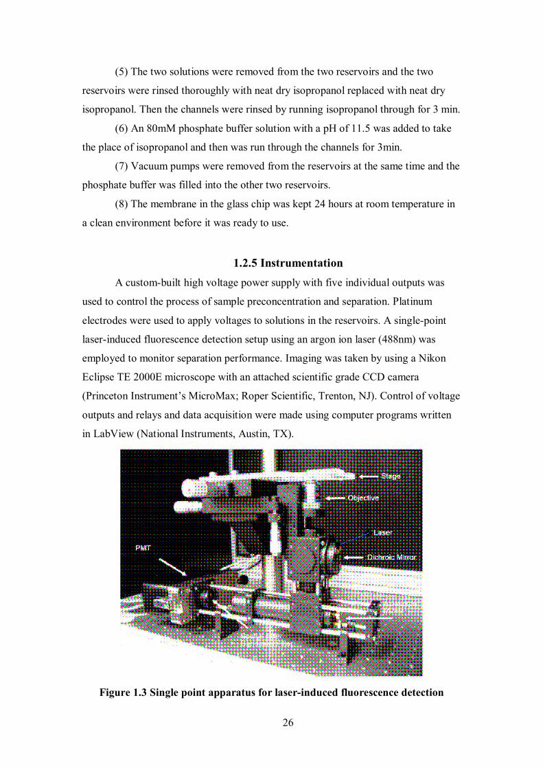
1.2.5 Instrumentation A custom-built high voltage power supply with five individual outputs was
used to control the process of sample preconcentration and separation. Platinum
electrodes were used to apply voltages to solutions in the reservoirs. A single-point
laser-induced fluorescence detection setup using an argon ion laser (488nm) was
employed to monitor separation performance. Imaging was taken by using a Nikon
Eclipse TE 2000E microscope with an attached scientific grade CCD camera
(Princeton Instrument’s MicroMax; Roper Scientific, Trenton, NJ). Control of voltage
outputs and relays and data acquisition were made using computer programs written
in LabView (National Instruments, Austin, TX).
Figure 1.3 Single point apparatus for laser-induced fluorescence detection

27
The home-made single point setup for fluorescence detection exploits an argon
ion laser (35-MAP-431-208; Carlsbad, California) as the excitation light, which has
the ability of producing 70mW laser lines at 488 nm and 514nm. The laser lines were
reflected off a 500 (or 560) nm long-pass dichroic mirror (500DRLP or 560DRLP)
(Omega Optical; Brattleboro, VT) and focused by a 40X objective (CD-240-M40X;
Creative Devices; Mechanic Station, NJ) into a small spot in a separation channel.
The excitation light from the fluorophore was collected by the same objective,
transmitted through the dichroic mirror and then spatially filtered using a 1mm
pinhole ( Oriel, Stratford, CT) and spectrally filtered by a bandpass filter(545 AF 75
or 595 AF 60; Omega Optical). A photomultiplier tube (PMT, R1477; Hamanatsu
Instruments, Inc.; Bridgewater, NJ) was used to detect and an SR 570 low noise
current preamplifier (Stanford Research Systems, Inc.; Sunnyvale, CA) with a 100HZ
lowpass filter was employed to amplify the signal which was subsequently sampled at
200Hz using a PCI-6036E multifunction I/O card (National Instruments, Inc.; Austin,
TX) in a computer. The program of Igor Pro of Labview was used to analyze all the
data for sample detection.
The optical parts such as bandpass filters and dichroic mirrors play very
important role in the sensitivity of the detection. Dichroic mirrors act as a beamsplitter
and are capable to reflect and transmit light by utilizing a large number of coating
techniques. They are used to transmit specific range of wavelengths through the filter
and reflect other range of wavelengths to obtain the desired wavelengths for detection.
1.3 Results and Discussion Silica membranes using sol-gel processing were already exploited on
microfluidic devices with different designs for sample preconcentration by Ramsey
(37-39). The formation of the silica membranes was accomplished in the process of
fabrication of the microchips. Photolithography and chemical wet etching were used
to transfer the microchip design onto the glass substrate. The bonding step of the glass
substrate and the cover plate was quite different from that in this work. A low-
temperature bonding process using a spin-on silicate adhesive layer as the adhesive
was applied to bond the cover plate and the glass substrate and form the enclosed
network of channels. Briefly, a silicate solution (usually potassium silicate) was
28
diluted with deionized water and then spin-coated onto the cover plate. Subsequently
the treated cover plate surface was brought into contact with the etched glass substrate
surface immediately. In this process, a narrow layer of porous silica membrane was
formed because of polycondensation of the silica sol-gel reaction and served as the
adhesive to connect the two surfaces. And then the bonded assembly was annealed at
200℃, which was utilized to strengthen the bonding through dehydration and siloxane
bond formation. The resulted semipermeable silica membranes, serving as a filter,
allowed passage of ionic current but blocked large molecules in this microchip design,
Therefore, it enabled and demonstrated preconcentration of protein and DNA samples
to achieve good separation and detection performance, as shown in the papers.
In our work, the purpose was to check on the function of a porous membrane
formed in situ in glass microchips with the different design (as indicated in Fig 1.1)
using a different sol-gel precursor of titanium metal alkoxide.
+300 V
+150 V+150 V
Ground
Concentrated spot
Figure 1.4 Schematic of membrane concentration on a glass chip
Fig 1.4 shows a schematic diagram of preconcentration. A high potential of
300 V was applied to the top reservoir. A potential of 150 V was applied to the two
side reservoirs individually which was used to prevent bleeding of the excess sample
into the separation channel ( the side channel to the right as indicated in Fig 1.5) in the
process of preconcentration. The bottom reservoir was connected to the ground. The
nanoporous property of the membrane combined with this voltage scheme allows

29
small buffer ions to pass through the porous membrane while prohibiting the passage
of large molecules. Therefore, large molecules can be accumulated at the top channel,
as indicated by the light blue spot.
Fig 1.5 presents preconcentration images for samples with different
concentrations taken by CCD camera using Winview 32 software. It can be seen
clearly that preconcentration effect was able to be achieved down to samples of
picomolar concentration. Fig 1.5 (d) depicts the image for a FITC-labeled amino acid
of arginine with a nanomolar concentration. Occasionally leakage of the concentrated
plug into the separation channel was observed. It might be due to imperfect
fabrication or breakdown of the membrane by applying the high potential difference
on the two sides of the membrane.
0 min 5 min 10 min
(a) Images for 0.3µM Standard fluorescein sample concentrated plug
(P.S. the different membrane position was because the mask was put upside down during
fabrication of the glass chip, which didn’t affect its usage.)
0 min 5 min
10 min
(b) Images for 1.36nM standard fluorescein sample concentrated plug
30
0 min
5 min
10 min
(c) Images for 3.2pM standard fluorescein concentrated sample plug
0 min 5 min
10 min
(d) Images for 1.2nM FITC labeled amino acid of arginine concentrated plug
Figure 1.5 Images of concentrated plugs for different samples generated
by membranes on glass chips: (a) 0.3µM standard fluorescein sample; (b) 1.36
nM standard fluorescein sample; (c) 3.2 pM standard fluorescein sample; (d) 1.2
pM FITC labeled arginine; All the samples were prepared using sodium
phosphate buffer at pH 11.5.
Fig 1.6 indicates the change of the fluorescence intensity of the preconcentrated
plug as a function of time during preconcentration of the sample of 1.36nM standard
fluorescein. From the plot, it can be seen that the fluorescence intensity demonstrated
almost a linear relationship with the preconcentration time. Combined with the images
shown in Fig 1.5, it can be seen that the titanium membrane fabricated within this

31
manifold performed very powerful ability of preconcentrating dilute samples down to
picomolar concentration.
0
2000
4000
6000
8000
10000
12000
14000
0 2 4 6 8 10 12
Time (min)
Fluo
resc
ence
Inte
nsity
Figure 1.6 Fluorescence intensity vs preconcentration time for 1.36 nM standard
fluorescein sample concentrated plug; Sodium phosphate buffer at pH 11.5 was
used.
A very interesting phenomenon was found during the preconcentration process.
Occasionally the preconcentrated sample plug was located at the right side of the
membrane instead of the top side or the left side, as shown in Fig 1.7. The sample
concentration used for this case was within the same level as that in Fig 1.5 (c), about
2.7pM standard fluorescein. In addition, comparing these two cases, very much higher
intensity was achieved for the second case. Two different membranes fabricated in
two glass chips were used for the two cases. For the second case, the position of the
membrane was closer to the right corner on the bottom of the intersection, as
indicated in Fig 1.8 i.e. n is much less than m. Therefore much more space was left
on the top of the membrane, which made it very difficult to form and hold the
concentrated sample plug. In contrast, the narrow spacing on the bottom of the
membrane was acting an obstacle for concentration. A reasonable explanation might
be made using the phenomenon of ion-enrichment and ion-depletion effect associated
with nanochannel structures developed and described in the literature (102). In this

32
phenomenon, both cations and anions were concentrated and depleted on the same
side of the nanochannel structures. In this case, it was assumed that the value of n
went down to the nanometer scale and thus the negatively charged fluorescein was
enriched on one side and depleted on the other side.
0 min 5 min 10 min
Figure 1.7 Images of concentrated plug generated by a membrane on a glass chip
for a second case; Sample: 2.7pM standard fluorescein in sodium phosphate
buffer at pH 11.5.
+300 V
+150 V+150 V
Ground
Concentrated spot
Figure 1.8 Schematic of membrane concentration on a glass chip for a second case
m
n
Separation voltage scheme is shown in Fig 1.9. The high voltage in the top
reservoir remained as 300 V, while all others were connected to the ground. As a
result, under the pumping of the electrokinetic driven, the concentrated plug moved to
the right channel as depicted by the block arrow in Fig 1.9. Then it would take a left
33
turn and get separated and detected. Sometimes the sample plug was too big to pass
through the intersection and move to the separation channel. It was struck at the
intersection. Therefore the optimized sample plug size and the optimized
concentration time should be the aim for the next step of research. Besides, the width
and the location of the membrane were critical for acquiring a very good
concentration sample plug and afterwards separation performance.
+300 V
GroundGround
Ground
Concentrated spot
Figure 1.9 Separation voltage scheme for concentrated samples
0.1cm
0.95cm
0.25cm
3.75cm
0.63cm
Detection
Figure 1.10 Schematic for detection position

34
Detection was made at the end of the channel connected to the reservoir at the
right side, as indicated by the green oval in Fig 1.10. Laser-induced fluorescence was
used for detection. The laser was focused at the detection point and was very critical
for obtaining a sharp peak with high intensity.
The separation result of a tentative trial made with a fluorescein standard
sample using the single point apparatus is given in Fig 1.11. The running conditions
for this trial were a sample of 0.3nM fluorescein in the buffer of sodium phosphate at
pH 11.5; preconcentration time of 5 min and a separation distance of about 1 cm. In
order to obtain very good peaks, further work for optimization of the preconcentration
and separation conditions is needed, such as concentration time, separation distance
and electric field strength.
1.2
1.0
0.8
0.6
0.4
0.2
Fluo
resc
ence
inte
nsity
150100500Time (sec)
Figure 1.11 Electrophoretic separation of 0.3 nM standard Fluorescein using the
voltage scheme indicated in Figure 1.9.

35
1.4 Conclusions and future work
To sum up, titanium membranes made on glass microchips in situ using
sol-gel chemistry have the ability to preconcentrate very dilute samples. Future work
will focus on the optimization of concentration and separation conditions using
standards such as proteins and amino acids in order to obtain very good separation
performance, such as preconcentration time, separation distance and separation
voltage. Then real samples will be used to check on the availability of this whole
system of membrane concentration, separation and detection within the glass
microchip.
36
Chapter 2 Protein Separations by CE using On-column
Fluorescence Labeling
Capillary electrophoresis includes a family of related separation techniques
conducted in buffer-filled, narrow-bore capillary tubes, usually with an internal
diameter (ID) between 25 and 100µm. It is a very efficient separation technique for
the analysis of a complex array of both large and small molecules. This technique was
originally invented by Arne Tiselius. In 1937, he successfully separated many
proteins in a tube by applying an electric field across the tube, which won him the
Nobel Prize in chemistry. Since then, capillary electrophoresis has been developed
and applied in many fields and demonstrated exceptional separation efficiency. The
fundamentals behind CE have been clarified. In 1989, the first fully automated
capillary electrophoresis instrument (P/ACE TM 2000) was introduced by Beckman
Instruments.
2.1 Principles of Capillary Electrophoresis (101, 103-105)
2.1.1 Electrophoretic Flow
Capillary electrophoresis is electrophoresis carried out in capillary tubes. The
principles that govern electrophoresis are directly applicable to CE. That the
differential movement or migration of ions is caused by attraction or repulsion under
the influence of an electric field results in the process of electrophoresis. Normally
for electrochemistry, when a negative (cathode) and a positive (anode) electrode are
immersed in a solution containing charged ions and then a potential difference is
applied across the two electrodes, ions of different charges will move towards the
electrode of opposite charge, i.e., positive ions (cations) move towards cathode while
negative ions (anions) move towards anode. Separations by electrophoresis are
operated by the fundamental that ions accelerate in an electric field resulting in

37
differences in ion velocities. In the process of electrophoresis, a balance between the
electric force and the drag or frictional force, also called a steady state, is obtained.
The electric force is expressed as
FE= qE
Where FE = electric force
q = ion charge
E = electric field strength
The drag force expression is given by
FF= -ƒν = -6πη rν
Where η = solution viscosity
r = ion radius
ƒ = friction coefficient
The electric force acts in favor of the ion movement while the retarding
frictional force slows down the ion motion. The ion almost instantly arrives at a
steady state velocity where the electric force equals the frictional force.
FE = -FF
Plug in the first two equations, the ion electrophoretic velocity expression will
be resolved as
νep= qE/(6π η r)
It can be seen clearly that the electrophoretic velocity of an ion is proportional
to its charge (q) and the electric field (E) and inversely in proportion to its radius and
the solution viscosity (η). Briefly, differences in the charge-to-size ratio of ions are
responsible for the differences in migration. An ion with a higher charge and a smaller
radius will migrate faster than an ion with a lower charge and larger radius. In
addition, the lower the solution viscosity, the higher the flow rate of an ion, and vice
versa. The ion charge can be affected by pH changes of the buffer. The ion radius can
be affected by the counter-ion present or by any complexing agents used. The
qualitative relationship can be defined as the term of electrophoretic mobility (µep),
µep = q/(6π η r )
Thus, electrophoretic velocity can also be expressed as,

38
νep=µep E
Electrophoretic mobility is a constant for a given ion and a given constant
buffer system. It indicates how fast a given ion may migrate through a given buffer
and determines migration velocity of an ion. The differences in electrophoretic
mobility are the basis for the separation of ion mixtures.
2.1.2 Electroosmotic Flow (EOF)
Electroosmosis refers to the movement of the bulk buffer solution in a
capillary tube under an electric field. For capillary electrophoresis, since an electric
field is applied through a narrow-bore fused-silica capillary tube used under most
conditions, a different form of ion movement occurs. Under aqueous conditions, the
ionizable silanol groups on the internal surface are easily ionized, leading to a
negatively charged surface along the capillary wall as indicated by the following
equation.
SiOH → SiO- + H+ (pH > 2)
This negatively charged surface is counterbalanced by positive ions in the
buffer, giving rise to an electric double layer and a potential difference (zeta potential)
close to the wall. As shown in Fig 2.1 by Stern’s model, the innermost layer of
positive ions is tightly bound to the surface and cannot move. It is also called the
compact layer or Helholtz or Stern layer, which can only neutralize the negative
charge. The second layer contains solvated, mobile positive ions which may diffuse
by thermal motion and neutralize the remaining negative charges. This charge double
layer creates a potential difference which is called zeta potential. The zeta potential is
the potential difference across the different part of the double layer and decreases
exponentially with increasing distance from the capillary wall surface. The zeta
potential is determined by surface charge density. For negatively charged silica
capillary surface, the surface charge density increases with increase in pH of the
buffer and decreases with increase in the ionic strength of the buffer, that is, the
concentration of the buffer. Under the influence of an electric field, the positive ions
in the diffuse layer migrate towards the cathode. Their movement will carry the bulk
39
buffer with them and lead to the bulk buffer flow towards the cathode too, which is
called electroosmotic flow. This pumping action is called electroosmosis. The
electroosmotic flow rate is expressed by
νeo = εζE/(4πη )
Where ε = dielectric constant of the buffer solution
ζ = zeta potential at the capillary and buffer interface
The equations of EOF are similar to those of electrophoresis. The
electroosmotic mobility can be described as
µeo = εζ/(4πη)
As the electrophoretic velocity does, the electroosmotic flow rate can also
be expressed as
νeo =µeo E
It can be seen that electroosmotic mobility is mainly affected by the dielectric
constant of the buffer solution, zeta potential and the buffer viscosity. It is
proportional to the dielectric constant, the zeta potential and inversely proportional to
the viscosity of the buffer. The zeta potential depends on the electrostatic nature of the
capillary surface, which is pH dependent, and the ionic strength of the buffer. At low
pH, EOF mobility is reduced because the charged SiO- is converted to neutral SiOH
by protons. It also decreases as ionic strength of the buffer increases because increase
in ionic strength can result in the compression of the double layer and thus the
decrease in zeta potential. EOF also can be reduced by using a material that is able to
suppress ionization of the silanol groups to modify the capillary wall surface.
Polyacrylamide and methylcellulose are examples of such materials.

40
Capillary wall
Inner layer Diffuse layer Bulk solution
Figure 2.1 Representation of the double layer charge distribution at the
capillary wall (Stern’s model)
2.1.3 Apparent Flow
The apparent migration velocity ,νapp, also can be called as electrokinetic
velocity ,νek , of an ion is a vector sum of the electrophoretic velocity, νep, and the
electroosmotic flow velocity, νeo, of the buffer.
νapp = νep +νeo
=µep E+ µeo E
= (µep +µeo) E
The apparent mobility, µapp, of the ion equals the vector sum of the
electrophoretic mobility, µep, of the ion and the electroosmotic mobility, µeo, of the
buffer.
µapp = µep + µeo
The apparent migration velocity can be rewritten as,
νapp =µapp E
One unique feature of EOF is that it leads to all the species- cations, anions
and neutrals moving in the same direction, from anode to cathode for negative
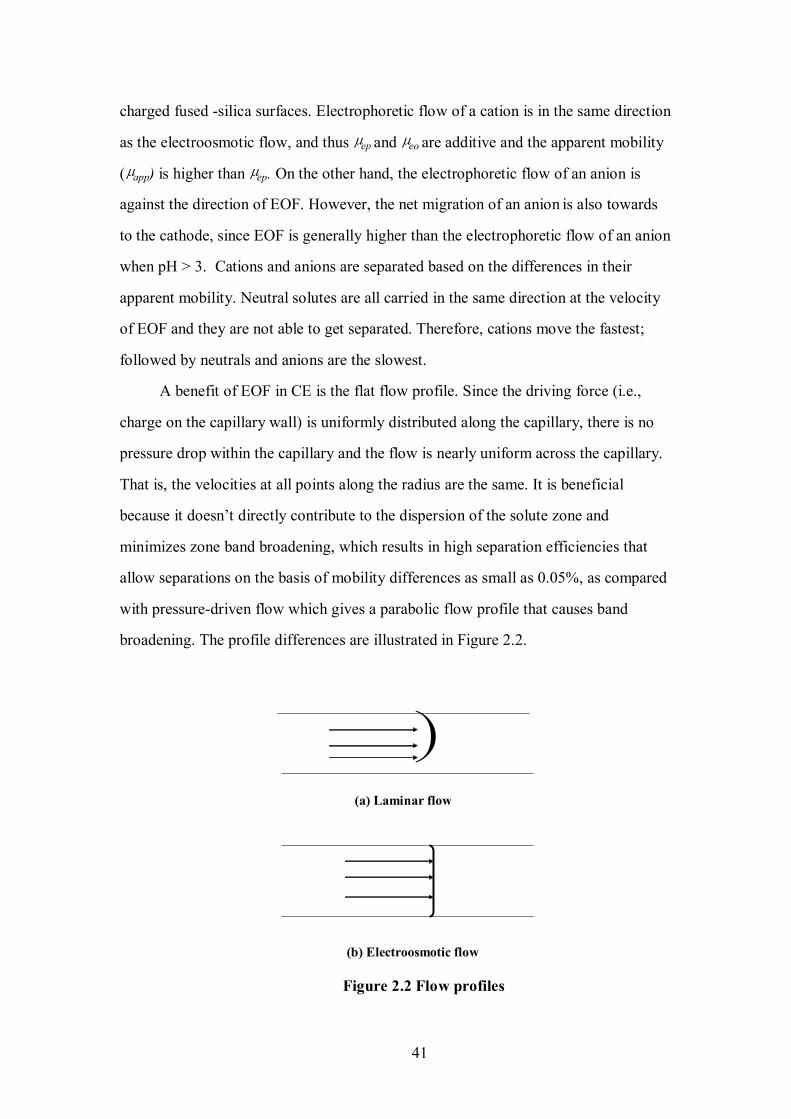
41
charged fused -silica surfaces. Electrophoretic flow of a cation is in the same direction
as the electroosmotic flow, and thus µep and µeo are additive and the apparent mobility
(µapp) is higher than µep. On the other hand, the electrophoretic flow of an anion is
against the direction of EOF. However, the net migration of an anion is also towards
to the cathode, since EOF is generally higher than the electrophoretic flow of an anion
when pH > 3. Cations and anions are separated based on the differences in their
apparent mobility. Neutral solutes are all carried in the same direction at the velocity
of EOF and they are not able to get separated. Therefore, cations move the fastest;
followed by neutrals and anions are the slowest.
A benefit of EOF in CE is the flat flow profile. Since the driving force (i.e.,
charge on the capillary wall) is uniformly distributed along the capillary, there is no
pressure drop within the capillary and the flow is nearly uniform across the capillary.
That is, the velocities at all points along the radius are the same. It is beneficial
because it doesn’t directly contribute to the dispersion of the solute zone and
minimizes zone band broadening, which results in high separation efficiencies that
allow separations on the basis of mobility differences as small as 0.05%, as compared
with pressure-driven flow which gives a parabolic flow profile that causes band
broadening. The profile differences are illustrated in Figure 2.2.
)(a) Laminar flow
(b) Electroosmotic flow
Figure 2.2 Flow profiles
42
Many methods have been reported to modify the internal surface of the fused
silica capillary to suppress EOF and reduce adsorption of solutes, such as covalent
attachment of silanes with neutral or hydrophilic components. The direction of EOF
can be reversed from cathode to anode by adding a positively charged surfactant like
cetyltrimethylammonium bromide (CTAB) to the buffer, since the surfactants form a
bilayer bound tightly to the negatively charged capillary wall and change the charge
of the wall from negative to positive.
2.1.4 Factors Affecting Separation
The van Deemter equation models separation efficiency of some separation
techniques such as chromatography including CE and field-flow fractionation.
H=A+B/υ+ Cυ
This equation relates the plate height (H) to the velocity (υ) of the carrier
gas or liquid along the separation axis. The lower is the value of H; the higher is the
separation efficiency. The terms of A, B and C are constants. The A term is the effect
of parabolic flow and multiple paths. It goes zero in CE due to the flat flow profile
resulted from EOF. The C term refers to mass transfer term and it also goes zero in
CE since no stationary phase exists and the separation is performed in a single liquid
phase. That is, two of the three contributing plate height terms in this equation are
eliminated. As a result, the longitudinal diffusion (B term) is the only source of band
broadening under ideal conditions. Under typical conditions, 50,000 to 500,000
theoretical plates count can be achieved by CE, which is an order-of-magnitude
higher than HPLC separation.
Band broadening refers to the process of dilution of analyte concentration as a
result that the different regions of the anayte migrate at different velocity. Diffusion is
the main source of band broadening. There are a number of other sources that might
contribute to band broadening and thus reduce separation performance. The sources
include sample injection volume, detection window length, adsorption,
electrodispersion, joule heating and so on (101).

43
A large sample injection volume can cause solute band broadening, especially
for fast separations in short capillary. The injection plug length should be controlled
less than 5% of the separation distance (i.e., the distance from the injection point to
the detection point).
Temperature variation due to joule heating produced by the resistance of the
bulk buffer to the flow of the electrical current in the capillary might affect the solute
band. The heat generated (H) equals the product of the applied voltage (V) and the
electric current (I) and the migration time (t).
H = VIt
The large surface to volume ratio of the capillary allows for the efficient heat
dissipation and application of high electric field. However if the heat dissipation is not
sufficient, especially under high electric field strength and some heat remains creating
a temperature gradient along the capillary radius. The temperature in the center along
the capillary radius is higher than that close to the capillary wall, leading to non-
uniformity of the buffer viscosity. The buffer in the center is less viscous than that
close to the capillary wall, resulting in a parabolic flow profile due to the non-
uniformity of analyte migration.
Electrodispersion is caused because of the fact that the conductivity of the
running buffer does not match that of the sample plug.
Long detection window is used to enhance the detection sensitivity, but it can
reduce the separation efficiency. Other factors such as analyte adsorption to the
capillary wall, laminar flow caused by the unequal buffer reservoir heights also
contribute to band broadening and thus degrade separation efficiency.
These factors including molecular diffusion are additive for peak width. Peak
width equals 4 times of the standard deviation of the peak (σ).
w = 4σ
The Einstein-Smoluchowski equation gives the σ expression caused by
molecular diffusion alone, which a Gaussian shaped analyte band is assumed.
σ2diffusion = 2Dt
The total standard deviation of the peak width can be described as

44
σ2total = σ2
diffusion + σ2injection + σ2
heating
+ σ2electrodispersion + σ2
detection window +σ2adsorption
In addition to plate height (H), peak width (w), other analytical parameters for
indicating CE separation efficiency contains theoretical plate count (N) and resolution
between two components (R). The relationship among these parameters can be
expressed as the following formula. Resolution is formulated by the difference in
baseline widths (w) and migration times of the two peaks.
N= ldet /H
= l2det /σ2
total
R= (t2-t1)/4σ
=2(t2-t1)/(w1+w2)
Theoretical plate counts indicates band broadening quantitatively. A high
value means the solute zone length is relatively short over a long separation distance,
indicating good separation performance, while a low number shows a poor separation.
For diffusion limited band broadening under ideal conditions, σ equals 2Dt.
D is diffusion coefficiency of the solute. T is migration time. L is capillary length, V
is applied voltage.
σ = 2Dt;
t = ldet /νapp;
νapp = µapp E;
E = L/V
From these formulas, the theoretical plate counts can be rewritten in terms of
the apparent mobility,
N =µapp Eldet /(2D)
Resolution between two components can be described as Rs = 0.25(µapp1- µapp2) {V/[2D(ūep+ µeo)]}1/2
It can be seen that a high theoretical plate count can be obtained by increasing
mobility, electric field strength and detection distance. A large difference in mobility
of the two components can help achieve good resolution.

45
2.2 Instrument of CE
CE system is very simple. Capillary tube and an electric field are needed for
CE operation. Capillary tube is the key part of CE system. Fused silica is commonly
used to produce capillary tube because of its intrinsic properties such as transparency
and high thermal conductance. The internal diameter of the capillary tube is normally
between 25-100µm. A high voltage power supply, normally between 0-30kV, is
needed. A diagram of CE system is indicated in Fig 2.3.
High voltage power supply
Fused silicacapillary
Detector
CathodeAnode
Data acquisition
EOF flow
Buffer reservoir
Figure 2.3 Schematic diagram of CE system
In the CE operation, the two ends of the capillary are connected to electrodes
through two separate buffer containers. The two electrodes are connected to the high
voltage supply. The capillary is first filled with the buffer. Then the analyte is
introduced into the capillary by replacing one of the buffer containers with the sample
reservoir. Normally the injection is made on the anode end. After the buffer container
is put back, a voltage is applied across the capillary and separation is carried out.
Usually detection, either on-column or off-column detection, is made near the cathode
end. Software packages are used to control the CE instrument.

46
2.3 Sample Injection
CE has the capability to inject extremely small volumes of a sample.
Normally the injection volumes fall in the range from picoliters to nanoliters. Either
electrokinetic or hydrodynamic injection can be employed. Electrokinetic injection is
conducted by simply applying a voltage for a certain time, usually within the range of
seconds. Many factors affect electrokinetic injection, such as injection time, voltage
and the property of the capillary wall. The following expression describes the relation
between the moles of each injected analyte (Qi) and the apparent velocity of each
analyte (νapp), the injection time (t), the ratio of conductivities of the buffer and the
sample (kb/ks). In the expression, r is the capillary radius and Ci is the molar
concentration of each analyte.
Qi = νapp (kb/ks)tπr2Ci
A problem associated with electrokinetic injection is the analyte dispersion
caused by the differences in mobility of different analytes. As a result, the
concentrations in the injected sample plug are different from those in the original
sample.
A pressure difference between the two ends of the capillary is applied to
achieve hydrodynamic injection. A pressure difference can be made by applying
vacuum. Siphoning also can be used to generate a pressure difference, simply by
raising the sample reservoir a certain height higher than the buffer reservoir on the
other end. The Poiseuille equation gives the volume of the injected sample.
Vc= ∆Pπd4t/128ηL
Where Vc = the calculated injection volume
∆P= pressure difference
d = inner diameter of the capillary
t = injection time
η = sample viscosity
L= capillary length

47
The sample injected by hydrodynamic injection is the same as the original
sample. However, in regard to precision and accuracy, electrokinetic injection is
more precise and accurate than hydrodynamic injection (106).The latter is less
reproducible. In addition, electrokinetic injection is easy to handle and the velocity
discrimination of the analytes during injection might contribute to selectivity (106).
2.4 Separation Modes of CE
CE can be divided into several separation techniques. The main examples
include capillary zone electrophoresis (CZE), capillary gel electrophoresis (CGE),
capillary isoelectric focusing (CIEF), micellar electrokinetic capillary
chromatography (MEKC), capillary isotachophoresis et al.
Capillary zone electrophoresis (CZE) is also named as free-solution CE
(FSCE). It is the simplest mode of CE family. Homogeneity of the running buffer and
constant field strength through the whole capillary are the fundamental of this mode.
The separation mainly depends on the pH modified dissociation of acidic groups or
the protonation of basic groups of analytes. A narrow zone of a sample is introduced
into the capillary, surrounded by the running buffer. As a voltage is applied across the
capillary, each analyte in the sample zone moves at a velocity based on its apparent
mobility. Under ideal conditions, each analyte will form an individual zone and get
separated from each other. All the neutrals will stay in one zone and separate from the
charged analytes, but they cannot separate from each other because they move at the
same flow rate as EOF.
Capillary gel electrophoresis (CGE) is adapted from the traditional slab gel
electrophoresis. It is carried out in a polymeric gel medium. The polymer network
serves as a sieve in which smaller molecules move quicker than large molecules by
decreasing the analyte diffusion velocity and the adsorption of the analyte to the
capillary wall. Since EOF is suppressed, short capillaries can be used, thus reducing
analysis time and increasing efficiency. Molecules are separated based on the
differences in their size in a nonconvective medium. CGE is very suitable for the

48
separation of large molecules like proteins and DNAs. Non-crosslinked polymer, such
as cellulose derivatives and polyacrylamide, and crosslinked gels, such as
polyacryamide and agarose can be used as gel media. Non-crosslinked polymers can
be easily removed out of the capillary and easily refilled to form a fresh capillary. By
modifying the concentration of the monomer and the degree of cross-linking for
crosslinked polymers, the resolution can be easily optimized.
Capillary isoelectric focusing (CIEF) is a separation form of CE on the basis
of differences in the isoelectric point (pI) of sample analytes. In this technique, a
charged analyte is driven through a pH gradient until it encounters a pH at which it
has a zero net charge and stops migration. Thus the analyte is focused into a tight
zone, which is then driven through the detector by pressure or chemical methods. If
the analyte molecules in the focused zone diffuse away from the zone, they will
immediately gain or lose protons and therefore obtain charges. The charged molecules
will be forced back to the zone center of the zero net charge point. A steady state in
which the zones are stationary and sharply focused will be reached in the end. The
expression of the variance of Gaussian distribution describes the width of the focused
zone.
σ2 = (D/E) (d(pH)/dµapp) (dx/pH)
To obtain a sharper zone, i.e., a smaller variance, a low diffusion coefficient
(D) and high field strength (E) is preferred. A high rate of change of mobility with pH
(dµapp / d(pH)) and a high slope of the pH gradient (d(pH)/dx) are favorable. A
difference between the two pIs required for a complete separation of two analytes
must be higher than 4σ.
A pH gradient is created using a series of zwitterions (ampholytes) under an
electric field. They are mixtures of 600-700 different zwitterionic compounds
exhibiting a series of pIs between 3 and 10. Positively charged ampholytes move
towards the cathode, while negative charged move to the anode, leading to an increase
of pH in the end of cathode and a decrease of pH at the anode end. When ampholytes
arrives at their own pI with a zero net charge, they discontinue migrating, generating a

49
stable pH gradient. A narrower pH range can be obtained using a large number of
ampholytes.
CIEF allows amphoteric molecules to be separated such as peptides, amino
acids and proteins. Free solutions or polymer gels can be used as the separation
medium. EOF and other convective forces should be eliminated or highly suppressed
in order to achieve effective CIEF. However, on the condition that the electrophoretic
velocity is greater than EOF, CIEF still can be conducted. One thing to pay attention
to is the pH of buffer electrolytes. In the cathode end, a buffer with a higher pH than
the pIs of all the basic ampholytes should be used, while a buffer with a lower value
of pH than the pIs of all the acidic amphoytes should be used in the anode end. Doing
this is to keeping buffers from migrating into the capillary from the buffer reservoirs.
Micellar electrokinetic capillary chromatography (MECC) can not only be
applied to separate charged compounds, but also neutrals. Micelles formed by adding
a micelle forming reagent to the separation buffer are used to serve as a pseudo-
stationary phase to separate neutrals. A micelle forming reagent is an amphiphilic
monomer (also called surfactant) which has a hydrophilic head and a hydrophobic
tail. The hydrophilic head can be cationic, anionic, nonionic or zwitterionic, while the
hydrophobic tail can be a straight or branched chain of hydrocarbon. Sodium dodecyl
sulfate is the most commonly used micelle forming reagent. When the concentration
of the micelle forming reagent is higher than its critical micelle concentration, the
molecules of the micelle forming reagent are aggregated together because of the
polarity of the buffer. In aqueous buffer, spherical micelles take the form of the
hydrophobic tails facing inside and the hydrophilic heads outside.
The separation principle in MECC is achieved by the combined result of the
differential partitioning of molecules between the buffer and the micelles and
differential migrations of ionic molecules. Analytes and micelles can interact with
each other through a number of types of forces such as hydrophobic, electrostatic and
H-bonding interactions. The neutral molecules migrate at the rate of EOF before the
micelles are added. The micelles move at a velocity lower than the EOF. When the
neutral is trapped by a micelle, it moves at the same velocity as the micelle. The

50
separation of analytes between the buffer and micelles can be adjusted by modifying
the concentration or the type of a surfactant. It also can be controlled by adding some
additives to the buffer such as ionic salts, chiral selectors; ion-pairing et al. Variation
in temperature and pH also affects separation. MEKC is very valuable in separating
mixtures of charged and neutral analytes.
Capillary isotachophoresis (CITP) is a separation technique using a moving
boundary electrophoretic mode. Two buffer solutions are used to generate a steady
state in which all analytes zones migrate at the same rate. The sample is added
between the leading buffer with a higher mobility and the trailing buffer with a lower
mobility compared with the mobility of the analytes. Differences in the velocities of
analytes in the sample zone are the basis for separation. After separation, each analyte
remains in different bands and move at the same rate, resulting in a steady state of
stacking. CITP cannot be utilized to separate both cations and anions in a single run.
Other modes of CE have been developed and applied, such as electrokinetic
chromatography (EKC), micro emulsion electrokinetic chromatography (MEEKC)
and capillary electrochromatography (CEC). Many combinations of different modes
of separation have been made for multidimensional separations, such as LC-CE,
CITP-CZE, IEC-CZE (IEC stands for ion-exchange chromatography) (107). Even
combinations of three separation techniques are available for 3-D separation system.
For example, Janini and coworkers have reported a powerful system of coupling IEF,
RP-HPLC and cation exchange chromatography which possesses the ability of
analyzing very complex mixtures (108). In two or multidimensional separation, IEP
and CITP modes are frequently utilized as the first step of preconcentration or/and
preseparation.
2.5 Methods of Detection for CE
Many detection methods have been combined with CE. Some commonly used
detection methods and their limit of detection (LOD) are listed in the table 1.1 of last
chapter.

51
UV-absorption detection is the universal method for monitoring CE
separations due to the strong absorption of a UV radiation (200-220nm). Laser-
induced fluorescence (LIF) possesses the highest sensitivity and has the potential to
detect even a single molecule. But LIF requires the derivatization of analytes, which
might result in multiple labeling and thus affect detection precision. The ideal
detection technique is mass spectroscopy which provides advantages of high
sensitivity and selectivity. It enables both analytical and structural determination. The
coupling of CE with MS has been growing. But the instrument of MS is very
expensive and the analysis costs much in terms of analysis time, sample consumption.
2.6 Applications of CE
CE has been highly accepted as an efficient separation technique for
qualitative determination. It offers advantages of simplicity, high resolution
separation, and minimal cost. CE operation is very rapid and takes little time. It
consumes little sample and reagents. Comparison of migration times with those of
standards is the best and simplest method to determine CE peaks qualitatively.
Additional information is needed for further confirmation. For example,
Spectrophotometric detection can be used to compare the ratio of absorbance at a
series of wavelengths in the unknown with the ratio in the suspected compound,
therefore giving further information for peak identity. In addition, amperometric
detection also can be employed to obtain the ratio of currents from two different
electrical potentials for further confirmation.
CE has not been fully established as a method of quantitative analysis.
However, it offers useful information about the concentration of an analyte in a
sample. Quantitative analysis can be achieved by comparing the analyte’s peak area
or height with those of calibration standards because peak height directly relates to the
concentration of the analyte and peak width directly relates to the residence time in
the detector. Internal standardization techniques using internal calibration have been
developed for quantitative analysis (109-111). It is aimed to reduce the sample bias

52
caused by electrokinetic injection and provides better precision. Normally, a known
concentration of an internal standard is added to the sample. The mixture is performed
by CE analysis; therefore the ratio of peak area or height of the analyte to that of the
internal standard can be obtained. A calibration curve should be prepared by plotting
ratios of peak area or height of the calibration standard to that of the internal standard
against the concentrations of the calibration standard.
A large number of papers about applications of CE have been published (107,
112-114). CE analysis has been applied in many fields such as biological and
pharmaceutical areas and has demonstrated tremendous potentials for a wide range of
compounds from small molecules, such as inorganic ions, organic acids, peptides,
drugs and nucleosides, to large compounds like proteins, hormones, nucleic acids. Its
application has even been extended to single cell analysis. Kvasnicka reviewed
applications of CE in food authentication which is used to check whether the
commercial food matches its description (112). A review on the recent advancement
of pharmacokinetic study using CE has been published by Sung (113). Kraly and
coworkers summarized bioanalytical applications of CE including single cell analysis,
neuroscience, DNA analysis, carbohydrates and lipids analysis (114). The detailed
applications of CE (including CEC) of peptides have been presented in the reference
106. The covered areas in this review contain quality control and determination of
purity, determination in biomatrices, monitoring of chemical and enzymatical
reactions and physical changes and amino acid sequence analysis et al.
2.7 Derivatization of Samples
As mentioned above, LIF is the most sensitive detection method and very
suitable for detection of very dilute samples. It is commonly combined with CE as a
detector. The fundamentals of fluorescence detection have been covered in the first
chapter. However, most biologically important compounds are not natively
fluorescent. The compounds that are natively fluorescent usually need high energy
excitation in the region of UV wavelengths such as the spectral region of 260-300nm

53
for aromatic amino acids or proteins containing aromatic amino acids. UV lasers in
this spectral region are very expensive and unreliable. Those limitations make it very
important to modify and label nonfluorescent compounds with a fluorescent labeling
reagent by chemical reactions to generate fluorescence in LIF (115). Fluorogenic
stains are another type of fluorescence labeling reagents. They are naturally
nonfluorescent reagents, but they can generate a fluorescent product when they react
with their target such as primary amines (116).
There are problems associated with fluorescence labeling reactions (116).
Under aqueous conditions, most fluorescent labeling reagents experience hydrolysis.
For an efficient labeling, the hydrolysis reactions make it necessary to use labeling
reagents with high concentrations. However, the use of high concentration of labeling
reagents and hydrolysis products lead to high background signal, suppressing the
fluorescence signal of analytes, especially very dilute samples. In addition, multiple
labeling is an intrinsic problem. Normally an analyte such as a protein possess many
labeling sites (primary amines for proteins). The labeling reactions don’t go to
completion, resulting in many different labeling products with different mobility,
therefore very complex broad peak profiles. To collapse multiple labeling, a reagent
(often a surfactant such as sodium dodecyl sulfate (SDS)) can be added to the sample
to form neutral reaction products along with an ion pair reagent to neutralize
unreacted labeling sites (117). The interaction between SDS and a protein occurs
through the hydrophobic attraction between the long alkane chain of SDS and the
hydrophobic regions of the protein, and the ionic interaction between the anionic
sulfate group of SDS and the positively charged side chains of unlabeled residues
(118). On the other hand, fuorogenic reagents can reduce the background by orders of
magnitude compared with fluorescent reagents. Therefore they are more suitable for
labeling very dilute samples.
Three labeling methods can be made for CE—precolumn, on-column and
postcolumn labeling. Precolumn labeling is the most common, but it consumes
relatively a large amount of analytes and labeling reagents. A postcolumn labeling
reaction goes slowly, thus limiting the detection. In contrast, on-column labeling is
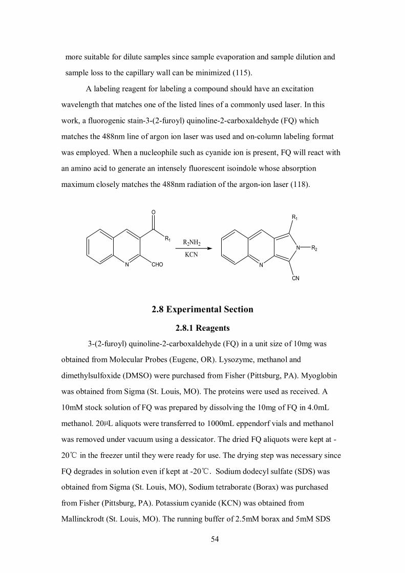
54
more suitable for dilute samples since sample evaporation and sample dilution and
sample loss to the capillary wall can be minimized (115).
A labeling reagent for labeling a compound should have an excitation
wavelength that matches one of the listed lines of a commonly used laser. In this
work, a fluorogenic stain-3-(2-furoyl) quinoline-2-carboxaldehyde (FQ) which
matches the 488nm line of argon ion laser was used and on-column labeling format
was employed. When a nucleophile such as cyanide ion is present, FQ will react with
an amino acid to generate an intensely fluorescent isoindole whose absorption
maximum closely matches the 488nm radiation of the argon-ion laser (118).
N
R1
O
CHO
R2NH2
KCNN
N
R1
R2
CN
2.8 Experimental Section
2.8.1 Reagents
3-(2-furoyl) quinoline-2-carboxaldehyde (FQ) in a unit size of 10mg was
obtained from Molecular Probes (Eugene, OR). Lysozyme, methanol and
dimethylsulfoxide (DMSO) were purchased from Fisher (Pittsburg, PA). Myoglobin
was obtained from Sigma (St. Louis, MO). The proteins were used as received. A
10mM stock solution of FQ was prepared by dissolving the 10mg of FQ in 4.0mL
methanol. 20µL aliquots were transferred to 1000mL eppendorf vials and methanol
was removed under vacuum using a dessicator. The dried FQ aliquots were kept at -
20℃ in the freezer until they were ready for use. The drying step was necessary since
FQ degrades in solution even if kept at -20℃. Sodium dodecyl sulfate (SDS) was
obtained from Sigma (St. Louis, MO), Sodium tetraborate (Borax) was purchased
from Fisher (Pittsburg, PA). Potassium cyanide (KCN) was obtained from
Mallinckrodt (St. Louis, MO). The running buffer of 2.5mM borax and 5mM SDS
55
with a pH of 9.5 was prepared for CZE analysis. A stock solution of KCN was made
in the running buffer at a concentration of 200mM. A 20mM solution of KCN was
prepared by 1:10 dilution using the stock solution. A stock solution of 0.8 mM
lysozyme and 1.0mM myoglobin was made using the running buffer. Then the stock
solution was diluted 1000-fold to get the µM solution using the running buffer. All
solutions were made with distilled, deionized water from a Barnstead Nanopure
System (Dubuque, IA) and then filtered by 0.45µm Acrodiscs (Gelman Sciences, Ann
Arbor, MI).
2.8.2 Instruments
Experiments were performed using an in-house built CE instrument with a LIF
detector. The LIF detector was described in detailed in the last chapter. The 488nm
beam of an argon ion laser was used as excitation.
2.8.3 Precolumn Labeling and CE Running Procedure
18µL of a sample solution and 2µL of the 20mM KCN solution were added to
a vial containing the dried FQ from 20µL aliquot and vortexed for 5s. The labeling
reaction was allowed from 10s to 1h.
Separations were carried out in a bare capillary by applying electric fields.
The polyimide coating was removed for detection by a gentle flame. Solutions were
injected by electrokinetic injection. The buffer of 2.5mM borax and 5mM SDS at pH
9.5 was used as the running fluid.
2.8.4 On-column Labeling and CE Running Procedure
The labeling reaction was performed in the capillary. The FQ solution was
prepared by adding 20µL of the running buffer to a vial of dried FQ. The protein/KCN
solution was made by adding 18µL of the protein solution and 2µL of the 20mM KCN
solution. Solutions were introduced hydrodynamically by a vertical displacement of
10cm for 20s. The protein and KCN solution was injected first and then followed by
the FQ solution. In between, the capillary tip was rinsed by dipping into a vial

56
containing the running buffer to minimize the contamination of the FQ solution.
Another vial containing the buffer heated to around 65℃ was used to hold the
capillary tip to improve efficiency of the labeling reaction. The labeling reaction was
allowed to react around 30s. Then a voltage was applied for separation. The buffer of
2.5mM borax and 5mM SDS at pH 9.5 was used as the running fluid.
Potassium cyanide (KCN) is very poisonous and generates lethal HCN gas
when encountering acids. A basic buffer should be used to prepare the stock solution
of KCN. Wastes containing KCN should be neutralized by a strong base solution such
as sodium hydroxide (NaOH) or Potassium hydroxide (KOH).
2.9 Results and Discussion
As discussed in the first section, theoretical plate number and resolution can
be expressed by the following two equations individually.
N =µapp Eldet/2D
Rs = 0.25(µapp1- µapp2){V/2D(ūep+ µeo)}1/2
It is clear that high separation efficiency can be achieved by increasing electric
field strength (E) and/or detection distance (ldet). Enhancing voltage may give a good
resolution. However, those variables cannot be raised without limitation. For example,
a longer detection distance leads to longer separation time, therefore wider peaks (σ =
2Dt). The resultant band broadening might cause poor resolution. In addition, an
applied high voltage may result in joule heating which contributes to band
broadening.
This work was aimed to find out the optimal running conditions for separation
using the home-made CE-LIF. FQ, a fluorogenic labeling reagent, was employed to
reduce fluorescent background. Techniques of precolumn and on-column labeling
were compared.
For the on-column labeling of FQ, at pH of 9.5, FQ is neutral while most
proteins are negatively charged. The apparent mobility of FQ is higher than those of
proteins. FQ moves faster than proteins. Thus FQ is introduced to the capillary first
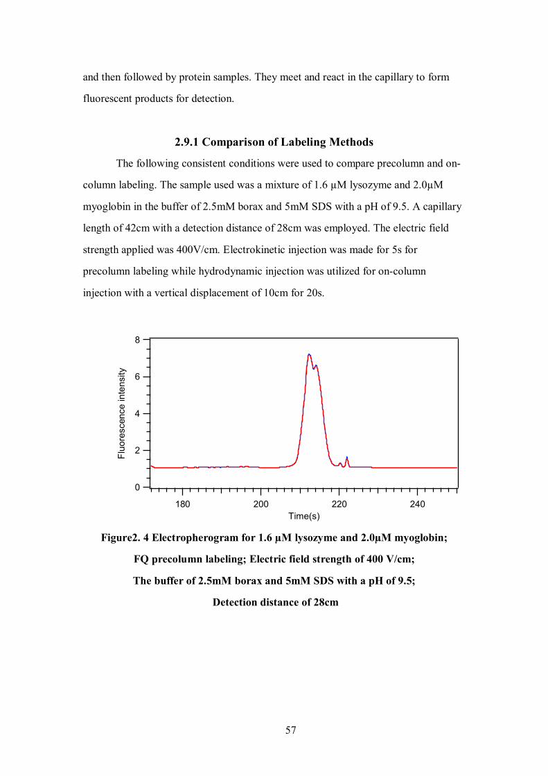
57
and then followed by protein samples. They meet and react in the capillary to form
fluorescent products for detection.
2.9.1 Comparison of Labeling Methods
The following consistent conditions were used to compare precolumn and on-
column labeling. The sample used was a mixture of 1.6 µM lysozyme and 2.0µM
myoglobin in the buffer of 2.5mM borax and 5mM SDS with a pH of 9.5. A capillary
length of 42cm with a detection distance of 28cm was employed. The electric field
strength applied was 400V/cm. Electrokinetic injection was made for 5s for
precolumn labeling while hydrodynamic injection was utilized for on-column
injection with a vertical displacement of 10cm for 20s.
8
6
4
2
0
Fluo
resc
ence
inte
nsity
240220200180Time(s)
Figure2. 4 Electropherogram for 1.6 µM lysozyme and 2.0µM myoglobin;
FQ precolumn labeling; Electric field strength of 400 V/cm;
The buffer of 2.5mM borax and 5mM SDS with a pH of 9.5;
Detection distance of 28cm

58
2.5
2.0
1.5
1.0
0.5
0.0
Fluo
resc
ence
inte
nsity
240220200180160Time(s)
Figure 2.5 Electropherogram for 1.6 µM lysozyme and 2.0µM myoglobin;
FQ on-column labeling; Electric field strength of 400 V/cm;
The buffer of 2.5mM borax and 5mM SDS with a pH of 9.5;
Detection distance of 28cm
It can be seen clearly that the two proteins were not resolved using precolumn
labeling under this condition, while much better resolution was obtained for on-
column labeling. Therefore for all the following runs, on-column labeling was taken.
Fig 2.6 gives the electropherogram for the blank (the solution of FQ with KCN
in water). The same running conditions and the exact running procedure as those of
Fig 2.5 were used.

59
1.0
0.8
0.6
0.4
0.2
0.0
Fluo
resc
ence
Inte
nsity
4003002001000Time(s)
Figure 2.6 Electropherogram for the blank of a solution of FQ and KCN in water
FQ on-column labeling; Electric field strength of 400 V/cm;
The buffer of 2.5mM borax and 5mM SDS with a pH of 9.5;
Detection distance of 28 cm
2.9.2 Comparison of Different Solvents for FQ
The solubility of FQ in water is limited. For 10mM FQ solution in water used,
some precipitates might be formed, which might have some negative influence on
separation performance. 5mM FQ solution was tried for on-column labeling scheme.
But probably because of the short on-column labeling reaction time and the difficulty
of mixing of FQ with samples on column, no good signal was obtained. In order to
increase the solubility of FQ without decreasing its concentration, DMSO was used as
a solvent to make 10mM FQ solution. No precipitate was observed. The separation
result was shown in Fig 2.7. The same running conditions were used as those of Fig
2.5 and Fig 2.6. It can be found that the intensity of the two peaks for DMSO is lower
than that for water as solvent. It might be partially because the solvents affected the
mobility of FQ and the labeling reaction in DMSO was not as adequate as that in
water. For the following experiment, water was used as the solvent for making the FQ
solution.

60
2.0
1.5
1.0
0.5
0.0
Fluo
resc
ence
Inte
nsity
250240230220210200Time(s)
Figure2.7 Electropherogram for 1.6 µM lysozyme and 2.0µM myoglobin;
FQ on-column labeling in DMSO; Electric field strength of 400 V/cm;
The buffer of 2.5mM borax and 5mM SDS with a pH of 9.5;
Detection distance of 28 cm
2.9.3 Comparison of Different Capillary Lengths
The separation performance of a longer capillary length of 60cm with a
detection distance of 40cm was compared with that of the former capillary with 42 cm
capillary length and 28cm detection distance. The following consistent conditions
were used: on-column labeling; the sample of 1.6 µM lysozyme and 2.0µM
myoglobin in the buffer of 2.5mM borax and 5mM SDS with a pH of 9.5 ; electric
field strength: 400V/cm; hydrodynamic injection: vertical displacement of 10cm for
20s.
The separation result using the 60cm capillary with 48cm detection distance
was given in Fig 2.8. Compared with Fig2.5, under the same electric field strength,
band broadening dominated separation at this longer capillary length. Very poor
resolution between the two components was observed. Therefore, for further
experiments, the 42cm length of capillary with 28 cm detection distance was used and
on-column labeling was taken.

61
0.5
0.4
0.3
0.2
0.1Fluo
resc
ence
inte
nsity
400350300250200Time(s)
Figure 2.8 Electropherogram for 1.6 µM lysozyme and 2.0µM myoglobin;
FQ on-column labeling; Electric field strength of 400 V/cm;
The buffer of 2.5mM borax and 5mM SDS with a pH of 9.5;
Detection distance of 48 cm
2.9.4 Comparison of Different Electric Field Strengths
The separation performance at the higher electric field strength of 500V/cm
was compared with that of 400V/cm whose separation result was given in Fig 2.5.The
following consistent running conditions were used: on-column labeling; the sample of
1.6 µM lysozyme and 2.0µM myoglobin in the buffer of 2.5mM borax and 5mM SDS
with a pH of 9.5; capillary length: 42cm; detection distance: 28cm; electric field
strength: 500V/cm; hydrodynamic injection: vertical displacement of 10cm for 20s.
Fig 2.9 gives the separation result at 500v/cm. It is seen clearly that at the
higher electric field strength, much better separation efficiency and much better
resolution were achieved. Approximately 1.4 million theoretical plate counts were
demonstrated. A separation resolution for the two proteins within the range of two
seconds was achieved.

62
6
5
4
3
2
1
0
Fluo
resc
ence
inte
nsity
166165164163162161160Time(s)
Figure 2.9 Electropherogram for 1.6 µM lysozyme and 2.0µM myoglobin;
Electric field strength of 500V/cm; FQ on-column labeling;
The buffer of 2.5mM borax and 5mM SDS with a pH of 9.5;
Detection distance of 28 cm
2.10 Conclusions and Future Work
On-column fluorescence labeling is a very feasible method for CE separation.
Under suitable experimental conditions, excellent separation performance with about
1.4 million theoretical plate numbers was achieved using on-column fluorescence
labeling.
Future studies will employ a mixture of more types of standard proteins with
different mobility to check on and further optimize the running conditions, such as
electric field strength, separation distance. Then real samples will be able to be
separated and analyzed using this setup and the optimized separation conditions.
63
CHAPTER 3 References
(1) Ouellette, J. The Industrial Physicist, August/September, 2003.
(2) Manz, A.; Graber, N.; Widmer, H.M. Sens. Actuaors 1990, B1, 244-248.
(3) Khandurina, J. etc. Anal.Chem. 2000, 72, 2995-3000.
(4) Manz, A. etc. Sens. Actuators 1990, B1, 249-255.
(5) Lab Chip, 2006, 6, 1118-1121.
(6) Snits, J.G. Sens. Actuators, A 1990, 21, 203-206.
(7) Esashi, M. Sens. Actuators, A 1990, 21, 161-167.
(8) Harrison, D.J.; Manza, A.; Fan, Z. H.; Ludi, h.; Widmer, H.M. Anal.Chem.
1992, 64, 1926-1932.
(9) AurouxP.A.; Iossifidis, D.; Reyes, D. R.; Manz, A. Anal.Chem. 2002, 74,
2637-2652.
(10) Jung, B.; Bharadwaj, R.; Santiago, J.G. Anal.Chem. 2006, 78, 2319-2327.
(11) Woolley, A.T.; Sensabaugh, G.F.; Mathies, R. A. Anal.Chem. 1997, 69,
2181-2186.
(12) Moore, A.W.; Jacobson, S.C.; Ramsey, J.M. Anal. Chem. 1995, 67, 4184-
4189.
(13) Von Heeren, F.; Verpoorte, E,; Manz, A.;Thormann, W. Anal.Chem.
1996, 68, 2044-2053.
(14) Roman, G.T., Hlaus,T., Bass, K.J., Seelhammer, T.G., Culbertson, C.T.
Anal.Chem. 2005, 77, 1414-1422.
(15) Kamholz, A.E., Weigl, B.H., Finlayson, B.A., Yager, P. Anal.Chem. 71,
5340-5347.
(16) Macounova, K., Cabrera, C.R., Holl, M.R., Yager, P. Anal. Chem. 72,
3745-3751.
(17) Hadd, A.G., Jacobson, S.C, Ramsey, J.M. Anal.Chem.71, 5206-5212
(1999).
(18) Sohn, L.L. et al. Proceedings of the National Academy of Sciences of the
United States of America 97, 10687-10690(2000).
(19) Cheng, S.B. et al. Anal. Chem. 73, 1742-1479(2001).
(20) Yang, T. L., Jung, S. Y., Mao, H.B., Cremer, P.S. Anal. Chem. 73,165-
169 (2001).

64
(21) Buchholz, B.A. et.al. Anal. Chem. 73, 157-164 (2001).
(22) Fan,Z.H. et.al. Anal.Chem. 71, 4851-4859 (1999).
(23) Glasgow, I.K. et.al. Ieee Transactions on Biomedical Engineering 48,
570-578(2001).
(24) Yang, J., Huang, Y., Wang, X.B., Becker, F.F., Gascoyne, P.R.C.
Anal.Chem. 71, 911-918 (1999).
(25) Folch, A., Jo, B.H., Hurtado, O., Beebe, D.J., Toner, M. J. Biom. Mate.
Research 52, 346-353 (2000). (26) Liang, Z.; Chiem, N.; Ocvirk, G.; Tang, T.; Fluri, K.; Harrison, D.J. Anal.
Chem. 1996, 68, 1040-1046.
(27) Chervet, J.P.; Van Soest, R.E.J.; Ursem, M. J. Chromtogr. 1991, 543,
439-449.
(28) Kutter, J.P.; Ramsey, R.S.; Jacobson, S.C.; Ramsey, J. M. J.
Microcolumn Sep. 1998, 10,313-319.
(29) Lichtenberg, J.; Verpoorte, E,;de Rooij, N.F. Electrophoresis 2001, 22,
258-271.
(30) Gong, M.; Wehmeyer, R.; Limbach, W.P.; Arias, F.; Heineman, W.
Anal.Chem. 2006, 78, 3730-3737.
(31) Pickering, L.W.; Baldock, S.J.; Fielden, P.R.; Goddard, N.J.; Snook,
R.D.; Btown, B. J.T. In Proceedings of Micro Total Analysis Systems, 1998, 101-104.
(32) VanderNoot, V.A.; Hux, G.; Schoeniger, J.; Shepodd, T. In Proceedings
of Micro Total Analysis Systems, 2001, 127-128.
(33) Figeys,D.; Aebersold, R. Anal.Chem. 1998, 70, 3721-3727.
(34) Kim,S.M.; Burns, M. Hasselbrink, E.F. Anal. Chem. 2006, 78, 4779-
4785.
(35) Mala, Z.; Krivankova, L.; Gebauer, P.; Bocek, P. Electrophoresis 2007,
28, 243-253.
(36) M.H.V. Mulder, Basic principles of Membrane Technology, 2nd edn,
Kluwer Academic Publishers, Dordrecht, The Netherlands, 2000.
(37) Khandurina, J.; Jacobson, S.C.; Waters, L.C.; Foote, R.S.; Ramsey, J.M.
Anal.Chem. 1999, 71, 1815-1819.
(38) Khandurina, J.; McKnight, T. E.; Jacobson, S.C.; Waters, L.C.; Foote,
R.S.; Ramsey, J.M. Anal.Chem. 2000, 72, 2995-3000.
65
(39) Foote, R.S.;Khandurina, J.; Jacobson, S.C.; Ramsey, J.M. Anal.Chem.
2005, 77, 57-63.
(40) Yu, C.; Davey,M.H.; Svec, F.; Frechet, J. M.J. Anal.Chem. 2001, 73,
5088-5096.
(41) Ikuta, K.; maruo, S.; Fujisawa, T.; Yamada, A. MEMS 1999, Orlando, Fl,
January 17-21, 1999; pp 376-381.
(42) Jong, J.de; Lammertink, R.G.H.; Wessling, M. Lab.Chip, 2006,6, 1125-
1139.
(43) Stafie, N.; Stamatialis, D.F.; Wessling , M. Sep. Purif.Technol., 2005,
45(3), 220.
(44) Wijmans, J.G.; Baker, R.W. J. Membr. Sci. 2005, 249, 245-249.
(45) Randall, G.C.; Doyle, P. Proc. Natl. Acad. Sci. U.S.A. 2005, 102(31),
10813-10818.
(46) Leclerc, E.; Sakai, Y.; Fujii, T. Biotechnol. Prog. 2004, 20, 750-755.
(47) Vollmer, A.P.; Probstein, R.F.; Gilbert, R., Thorsen, T. Lab. Chip. 2005,
5(10), 1059-1066.
(48) Leach, A.M.; Wheeler, A.R.; Zare, R.N. Anal. Chem. 2003, 75, 967-972.
(49) Ro, K.W.; Lim, K.; Kim, H.; Hahn, J.H. Electrophoresis 2002, 23, 1129-
1137.
(50) Eijkel, J.; Bomer, J.; Van den Berg, A. Appl. Phys.Lett. 2005 87, 103-114.
(51) Su, Y.C.; Lin, L. J. Microelectromech. Syst. 2004 13(1), 75-82.
(52) Wang, P.C.; DeVoe, D.L.; Lee, C.S. Electrophoresis 2001, 22, 3857-
3867.
(53) Jiang, Y.; Lee, C.S. J. Chromatogr., A, 2001, 924(1-2), 315.
(54) Wang, P.C.; Gao, J.; Lee, C.S. J. Chromatogr., A, 2002, 942,115-122.
(55) Metz, S.; Trautmann, C.; Bertsch, A.; Renaud, P. J. Micromech.
Microeng., 2004, 14, 324-331.
(56) Kelly, R.T.; Li, Y.; Woolley, A.T. Anal.Chem. 2006, 78 (8), 2565-2570.
(57) Heyderman, L.J.; Ketterer, B.; Bachle, D.; Glaus, F.; Haas, B.; Schift, H.;
Vogelsang, K.; Gobrecht, J.; Tiefenauer, L.; Dubochet, O. Microelectron. Eng. 2003,
67-68,208.
(58) Cui, T.; Fang, J.; Zheng, A.; Jones, F.; Reppond, A. Sens. Actuators, B,
2000, 71, 228-231.

66
(59) Yegung, K.L.; Zhang, X.; Lau, W.N.; Martin-Aranda, R. Catal. Today,
2005, 110 (1-2), 26.
(60) Tjerkstra, R.W.; Gardeniers, J.G.E.; Kelly, J.J.; Van den Berg, A.
J.Microelectromech. Syst., 2000, 9 (4), 495-501.
(61) Moorthy, J.: Beebe, D.J.; Lab Chip, 2003, 3(2), 62-66.
(62) Song, S.; Singh, A.K.; Kirby, B.J.; Anal.Chem., 2004, 76,4589-4592.
(63) Song, S.; Singh, A.K.; Shepodd, T.J.; Kirby, B.J.; Anal.Chem., 2004, 76,
2367-2373.
(64) Hisamoto, H.; Shimizu, Y.; Uchiyama, K.; Tokeshi, M.; Kikutani, Y.;
Hibara, A.; Kitaori, T.; Anal. Chem., 2003, 75, 350-354.
(65) Malmstadt, N.; Nash, M.A.; Purnell, R.F.; Schmidt, J.J. Nano Lett. 2006,
6 (9), 1961-1965.
(66) Moskvin, L.N.; Gurskii, V.S. Zh. Anal. Khim., 1988, 43(4), p581.
(67) Moskvin, L.N.; Nikitina, T.G. Membrane, Ser. Krit. Tekhnol., 2000, 8, p3
(68) Van de Nerbel, N.C.; Hajeman, J.J.; Brinkman, U.A.Th., J. Chromatogr.,
1993, 634, 1.
(69) Van de Nerbel, N.C.; J. Chromatogr., 1999, 856, p55.
(70) Valcarcel, M., Arce, L., Rios, A., J. Chromatogr., 2001, 924, p.3.
(71) Moskvin, L.N.; Nikitina, T.G. J.Anal.Chem. 2004, 59(1), 2-16.
(72) Lichtenberg, J.; De Rooij, N.F.; Verpoorte, E. Talanta, 2002, 56(2), 233-
266.
(73) Peterson, D.S. Lab Chip, 2005, 5, 132-139.
(74) Handbook on biopolar membrane technology, ed. A.J.B. Kemperman,
Twente University Press, Enschede, The Netherlands, 2000.
(75) Klein, L.C. Noyes, Park Ridge, N.J., 1988, p.382.
(76) Avnir, D. Acc. Chem. Res. 1995, 28,328
(77) Lev, O.; Tsionsky, M.; Rabinovich, L. Glezer, V.; Sampath, S.;
pankratov, I.; Gun, J. Anal. Chem. 1999, 67, 22A.
(78) Collinson, M.M. Crit. Rev. Anal. Chem. 1999, 29, 289.
(79) Brinker, C.J.; Scherer, G.W. Sol-gel Sceince. Academic: New York,
1989, P2.
(80) Martin-Brown, S.; Collinson, M.M. Thesis of M.S. KSU, 2004.
(81) Malik, A. Electrophoresis 2002, 23, 3973-3992.
(82) Hench, L.L.; West, J.K. Chem. Rev. 1990.90.33.

67
(83) Brinker, C.J.; Scherer, G.W. Sol-gel Sceince. Academic: New York,
1989, P.460.
(84) Ibid, p.465.
(85) Ibid, p.469.
(86) Brinker, C.J.; Scherer, G.W. Sol-gel Sceince. Academic: New York,
1989, P453.
(87) Nogami, M.; Suzuki, S.; Nagaska, K. J. Non-cryst. Solids 1991, 135,182.
(88) Avnir, D.; Braun, S.; Lev, O.; Ottolenghi, M. Chem. Mater. 1994, 6,
1605.
(89) Lai, D.C.; Dunn, B.; Zink, J.I. Inorg. Chem. 1996, 35, 2152.
(90) Darder, M.; Colilla, M.; Lara, N.; Ruiz-Hitaky, E. J. Mater. Chem. 2002,
12, 3660.
(91) Guizard, C. Fundamentals of inorganic membrane science and
technology; Elsevier Science B.V. 1996.
(92) Collinson, M.M. Mikrochim.Acta 129, 1998, 149-165.
(93) Schubert, U.; Husing,N.; Lorenz, A. Chem. Mater. 1995, 7, 2010.
(94) Collinson, M.M. Trends Anal. Chem. 2002, 21, 30.
(95) Celzard, A.; Mareche, J.F. J.Chem. Educ. 2002, 79,854.
(96) Brinker, C.J.; Ward, T.L.; Sehgal, R.; Raman, N.K.; Hietala, S.L.; Smith,
D.M.; Hua, D.W.; Headley, T.J. J.Membr. Sci., 1993, 77, 165.
(97) De Lange, R.S.A. et al. J. Sol-Gel Sci.Tech., 1994, 2, 489.
(98) Guizard, C.; Cygankiewicz, N.; Larbot, A.; Cot, L. J.Non-Cryst. Solids,
1986, 82, 86.
(99) Guizard, C.; Larbot, A.; Cot, L.; Perez, S.; Rouviere, J.; Etude de la.
J.Chim. Phys., 1990, 87, 1901.
(100) Brinker, C.J.; Sehgal, R.; Raman, N.; Schunk, P.R.; Headley, T.J. J.Sol-
Gel Sci. Techol.; 1994,2,469.
(101) Khaledi, M.G.; High Performance Capillary Electrophoresis; John
Wiley&Sons, NY, 1998.
(102) Pu, Q; Yun, J; Temkin, H; Liu, S. Nano Lett., 2004, 4, 1099-1103.
(103) Camilleri, P. Capillary Electrophoresis: Theory and Practice; CRC
Press; Boca Raton, 1993.

68
(104) Kuhn, R.; Hoffstetter-Kuhn, S. Capillary Electrophoresis: Principles and
Practice; Springer-Verlag: Berlin, 1993.
(105) Landers, J.P. Handbook of Capillary Electrophoresis; CRC Press: Boca
Raton, 1994.
(106) leube, J.; Roechel, O. Anal.Chem. 1994, 66, 1090.
(107) Kasicka, V. Electrophoresis 2006, 27, 142-175.
(108) Janini, G.M.; Conrads, T.P.; Veenstra, T.D.; Issaq, H.J.; J. Chromatogr.
B 2003, 787, 43-51.
(109) Fujiwara, S.; Honda, S. Anal. Chem. 1986, 58, 1811-1814.
(110) Huang, X.; Luckey, J. A.; Gordon, M.J.; Zare, R. N. Anal. Chem. 1989,
61, 766-770.
(111) Dose, E.V.; Guiochon, G.A. Anal. Chem. 1991, 63, 1154-1158.
(112) Kvasnicka, F. J.Sep.Sci. 2005, 28, 813-825.
(113) Sung, W.; Chen, S. Electrophoresis 2006, 27, 257-265.
(114) Kraly, J.; Fazal, M.A.; Schoenherr, R.M.; Bonn, R.; Harwood, M.M.;
Turner, E.; Jones, M.; Dovichi, N.J. Anal. Chem. 2006, 78, 4097.
(115) Ahmadzadeh, H.; Krylov, S. Methods in Mol. Bio. 276, 29-38.
(116) Pinto, D.M.; Arriaga, E. A.; Craig, D.; Angelova, J.; Sharma, N.;
Ahmadzadeh, h.; Dovivhi,N.J. Anal.Chem. 1997, 69, 3015-3021.
(117) Hu, Sh., Dovichi, N.J. Current opinion in Chem. Bio. 2003, 7, 603-608.
(118) Beale, S., Hsieh, Y., Wiesler, D. Novotny, M. J. Chrom. 1990, 499, 579-
587.