EE368: Digital Image Processing

FACE DETECTION

Siddharth Joshi, Gaurav Srivastava sidj@stanford.edu, gauravs@stanford.edu

Abstract

Human face detection has become a major field of interest in current research because there is no deterministic algorithm to find face(s) in a given image. Further the algorithms that exist are very much specific to the kind of images they would take as input and detect faces. The problem is to detect faces in the given, colored class group photograph. The approach, we take is a mixture of heuristic and known algorithms. To detect faces we can put a number of simple rejection blocks in series, until we get the faces. Deeper the rejection block, more specifically it can be trained to eliminate non-faces. Various methods like neural networks, template matching, maximal rejection, fisher linear discriminants and eigenfaces have been tried. Finally, a combination of skin color segmentation, morphological operations (erosion), and eigenfaces has been used. 1. Introduction A face detection algorithm is very specific to the kind of problem and cannot be guaranteed to work unless it is applied and results are obtained. We have followed a multiple algorithm approach for face detection, which is in effect a series of simple rejection blocks. In designing the final algorithm many different schemes have been tried. The first step is skin segmentation, which is good enough to reject most of the data. Thus this forms the first step of the final algorithm also. Neural networks have also been applied (which is described later) but have not been included in the final algorithm. As the data gets more compact and we need more specific rejection classifiers. Fisher Linear Discriminants and Template matching are found not to perform as well as eigenface method. So in the final version we used eigenface projection method. In the overall algorithm there are many parameters that have to be decided by experimenting, and are chosen with respect to optimality of result, runtime etc.

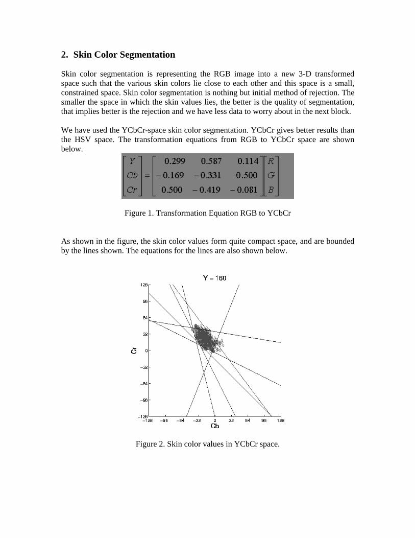
2. Skin Color Segmentation Skin color segmentation is representing the RGB image into a new 3-D transformed space such that the various skin colors lie close to each other and this space is a small, constrained space. Skin color segmentation is nothing but initial method of rejection. The smaller the space in which the skin values lies, the better is the quality of segmentation, that implies better is the rejection and we have less data to worry about in the next block. We have used the YCbCr-space skin color segmentation. YCbCr gives better results than the HSV space. The transformation equations from RGB to YCbCr space are shown below.

Figure 1. Transformation Equation RGB to YCbCr As shown in the figure, the skin color values form quite compact space, and are bounded by the lines shown. The equations for the lines are also shown below.

Figure 2. Skin color values in YCbCr space.

Figure 3. Equation in YCbCr space that bound the skin values This skin segmentation does well in marking out the areas where there is actually skin, i.e. faces, hands etc. But it also marks the points on unwanted objects like the wall, the bar, trees, skin colored jackets etc. These false positives do cover a lot of area as compared to the actual skin 3. Neural Networks The neural network is based on histogram approach rather than directly training the neural network of a fixed size image. The neural network first converts the RGB image to YES space. The equations for the conversion are shown below. The transformed skin color values have the E, S component close to zero.

=

B

G

R

. -. .

. . -.

. . .

S

E

Y

500025002500

000050005000

063068402530

.

Figure 4. Transformation Equation RGB to YCbCr

The neural network takes input as an image, much smaller than a group photograph, usually a size which contains a single face; and tell whether the given image has a face or not. We feed the neural network with blocks cut from the given image and then according to the output keep the image for further processing otherwise reject the block. Exact

details are described later. The given image (or block of image) is first converted to YES space. And then histograms are constructed for each of the dimensions. These histograms values are fed to the neural network. The number of histograms decides the complexity of the neural network. We have kept his value at 20. Still the neural operation is expensive in consideration with time, we must judiciously determine the inputs to the neural network. Since we have the marked skin segment data, we can use this information (leave the unmarked blocks) to cut out blocks and give them as input to the neural network. This operation also cannot be done for every pixel which has been marked. So we go through the image in blocks of size 25X25. Further the input block to the neural has a size or around 60X90, which when checked as face is not fed again to the neural, even if we traverse the lower part again. And if is detected to be a non-face we clear the 25X25 or a 25X50 block. This neural network eliminated quite a good amount of false skin marked data. It almost never loses a face, but objects like wall and jackets are also detected.

Figure 5. A sample run of neural network on the image.

In the final version of the algorithm we have not used the neural network as we emphasized more on morphological operation.

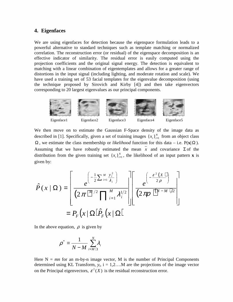
4. Eigenfaces We are using eigenfaces for detection because the eigenspace formulation leads to a powerful alternative to standard techniques such as template matching or normalized correlation. The reconstruction error (or residual) of the eigenspace decomposition is an effective indicator of similarity. The residual error is easily computed using the projection coefficients and the original signal energy. The detection is equivalent to matching with a linear combination of eigentemplates and allows for a greater range of distortions in the input signal (including lighting, and moderate rotation and scale). We have used a training set of 53 facial templates for the eigenvalue decomposition (using the technique proposed by Sirovich and Kirby [4]) and then take eigenvectors corresponding to 20 largest eigenvalues as our principal components.

10 20 30 40 50 60

10

20

30

40

50

60

10 20 30 40 50 60

10

20

30

40

50

60

10 20 30 40 50 60

10

20

30

40

50

60

10 20 30 40 50 60

10

20

30

40

50

60

10 20 30 40 50 60

10

20

30

40

50

60

Eigenface1 Eigenface2 Eigenface3 Eigenface4 Eigenface5 We then move on to estimate the Gaussian F-Space density of the image data as described in [1]. Specifically, given a set of training images N

ttx 1 = from an object class

Ω , we estimate the class membership or likelihood function for this data – i.e. P(x| Ω ).

Assuming that we have robustly estimated the mean x and covariance Σ of the distribution from the given training set N

ttx 1 = , the likelihood of an input pattern x is

given by:

( )

( )

( )( )

=Ω −

−

=

−

∏

=

2

2

1

212

2

1

22)|(ˆ

2

1

2

MN

X

M

i iM

y

eexP

M

ii

i

πρλπ

ρε

λ

( ) ( )ΩΩ= |ˆ| xPxP FF In the above equation, ρ is given by

+=−

=N

MiiMN 1

* 1 λρ

Here N = mn for an m-by-n image vector, M is the number of Principal Components determined using KL Transform, yi, i = 1,2….M are the projections of the image vector on the Principal eigenvectors, )(2 Xε is the residual reconstruction error.

( )Ω|xPF is the true marginal density in F-space and ( )Ω|ˆ xPF is the estimated marginal

density in the orthogonal complement F -space.

The density estimate )|( Ω∧

xP can be used to compute a local measure of the target saliency at each spatial position (i,j) in an input image based on the vector x obtained by lexicographic ordering of the pixel values in a local neighborhood Rij – i.e. S(i,j;Ω ) =

)|( Ω∧

xP where x is the vectorized region Rij. The Maximum likelihood estimate of the target Ω is given by

);,(maxarg),( Ω= jiSji ML

We have used this estimate to detect the center of faces in a given input image since the ML criteria using facial eigenvectors will give a peak typically somewhere around the nose of the face.

Figure 6. Detected Face

Figure 7. Probability Density

We have also used the RMS reconstruction error as our criteria for differentiating face from a non-face based on the assumption that a face image reconstructed from 20 principal components will have a very small MSE as compared to a non-face reconstructed from the PCA vectors.

Figure 8. Reconstruction Error for faces and non-faces Eigenfaces are primarily used for face recognition and therefore if we pass a block with few images, say one or two, then we have a good chance of finding the face, in fact the face centers. But if a larger block containing several faces is passed to the eigenface routine it may not perform that well; both in terms of the final output and the total time taken. We have to find a method by which we could separate out the blocks.

Gender Determination using Eigenfaces: For this task, we used a training subset of images containing only the faces of females and projected them onto the principal eigen vectors to obtain a set of projections. Whenever we get a face candidate in the input image, we calculate it’s projection on the principal eigen vectors and find the MSE between this projection and the projections stored for a female face. When MSEs are calculated for all the face candidates, the face candidate with the lowest MSE is declared as the female.

For a female Fi , if the training images are Ti1, Ti2, …… Tik then we obtain the set of projections as

)( Ψ−Φ= ikTMik Ty

where TMΦ is the matrix containing principal eigen vectors and Ψ is the mean image of

the training set. Whenever we have a face candidate x, we find it’s projection xy similar

to above and find the MSE as

=

−−=k

iikx

Tikxx yyyyMSE

1

)()(

If a face x~ is such that )min(~ xx MSEMSE = then we decide that x~ = Fi.

5. Erosion Consider a binary image formed by making the skin marked values as 1 and others as zeros. Some faces that are far apart will form a separate cluster and just this block can be separated from the rest of the image. I series of erosion operations should allow us to break big blocks. After each erosion step when we find a block of suitable size then we can run the eigen function on the block to find faces. The type of structuring element for erosion is important, as it should not eat up small faces. For this we initially apply hole filling, which fills the eyes and mouth region, so that while erosion these holes do not become big and eliminate the face. Once a block in the binary image is selected, the block which is passed to the eigen function is a rectangle from the working image bounded by maximum and minimum of a pixel that has the same label value as the selected block. Once a block has been selected, and is passed thru the eigen function, the block is will be blacked out in the working image. This will make sure that once a face has been passed will not be passed again as it will be blacked out and thus, will not cause interference in the future. The particular pixels having the label are also eliminated or assigned value 0 in the binary image. The number of erosion steps was decided to be three. Our method can be described as follows:

• Skin segmentation • Hole fill • Erosion 1, S.E.: diamond • Bwlabel • Select blocks size > Th11 & < Th12 • Erosion 2, S.E.: vertical bar • Bwlabel • Select blocks size > Th21 & < Th22 • Erosion 3, S.E.: vertical bar • Bwlabel • Select all remaining blocks

6. Heuristics The important part of the procedure is the heuristic, i.e. the manner in which the algorithms described above are used. Many parameters were decided by experimenting with the images and finding the optimum value. • For the skin color segmentation we ignore 50 columns from the side, and nearly

1/3rd image from the bottom. Since they (all seven training images) did not loose a face, this approximation is good enough. It immediately reduces our search space, without any effort.

• After the skin color segmentation there are lots of spots in the tree, bar etc where

there is no skin, but is include by the skin segmentation method. But these spots are not as dense as most of the spots on the faces. (Spot on walls are dense). Erosion and then dilation does remove the spots and we use do not use neural in our final version.

• The function which detects the faces using eigenface criteria also uses a scanning

block whose size is made appropriate by experimenting with various block size. The step size by which the block moves is decided in the same manner.

• The thresholds for the block size that are selected after erosion are such values

which will at least contain a face and also not too many faces. Th11 has a value of 2,000 pixels and Th22, 20,000.

7. Results We show the image at various stages of the algorithm. 1. Original Image

Figure 9. Image 6 of the Training Set

2. Image After Skin Segmentation

Figure 10. Result of Skin Segmentation

3. Binary image

Figure 11. Binary Image formed by skin segmented region

4. Image after the erosion steps.

Figure 12. Image 3 of the Training set after the erosion steps.

The various colors show the order in which the blocks are operated upon. After the first erosion step all green blocks are given to the eigen function. After the second erosion all the blue blocks, and finally the cyan blocks are processed.

5. The final image.

Figure 13. Image marked with output of the algorithm The square is marked around the output values of the function. In the above image

• 22 faces detected. • 2 false alarms. • 2 miss detections.

The values that are detected as female, are marked by a yellow square. In the above image these values are correct.

8. References [1] Moghaddam B. and Pentland A., “Probabilistic Visual Learning for Object

Detection,” Vision and Modeling Group, The Media Laboratory. M.I.T. [2] O’Toole, Abdi, Deffenbacher and Valentin, “Low-dimensional representation of faces

in higher dimensions of the face space,” School of Human Development, The University of Texas at Dallas.

[3] Turk M. and Pentland A., “Eigenfaces for Recognition,” Media Labs, M.I.T. [4] Kirby M. and Sirovich L., “Application of Karhunen-Loeve Procedure for the

Characterization of Human Faces,” IEEE Transaction on Pattern Analysis and Machine Intelligence, Vol 12, No. 1, January 1990.

[5] Garcia C. and Tziritas G., “Automatic Face Detection in Complex Color Images,”

http://www.csd.uch.gr/~cgarcia/FACE/Face.html [6] Whittman T. and Shen J., “Face Detection and Neural Networks,”

http://www.math.umn.edu/~wittman/faces/main.html