factor analysis - university of alabama

Factor Analysis Principal components factor analysis Use of extracted factors in multivariate dependency models

Notes on Factor Analysis: Charles M. Friel Ph.D., Criminal Justice Center, Sam Houston State University

2

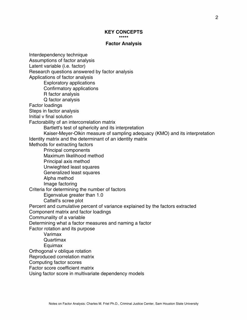
KEY CONCEPTS *****

Factor Analysis Interdependency technique Assumptions of factor analysis Latent variable (i.e. factor) Research questions answered by factor analysis Applications of factor analysis Exploratory applications Confirmatory applications R factor analysis Q factor analysis Factor loadings Steps in factor analysis Initial v final solution Factorability of an intercorrelation matrix Bartlett's test of sphericity and its interpretation Kaiser-Meyer-Olkin measure of sampling adequacy (KMO) and its interpretation Identity matrix and the determinant of an identity matrix Methods for extracting factors Principal components Maximum likelihood method Principal axis method Unwieghted least squares Generalized least squares Alpha method Image factoring Criteria for determining the number of factors Eigenvalue greater than 1.0 Cattell's scree plot Percent and cumulative percent of variance explained by the factors extracted Component matrix and factor loadings Communality of a variable Determining what a factor measures and naming a factor Factor rotation and its purpose

Varimax Quartimax Equimax Orthogonal v oblique rotation Reproduced correlation matrix Computing factor scores Factor score coefficient matrix Using factor score in multivariate dependency models


3

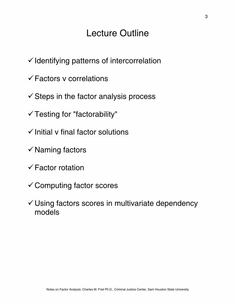
Lecture Outline

Identifying patterns of intercorrelation

Factors v correlations

Steps in the factor analysis process

Testing for "factorability"

Initial v final factor solutions

Naming factors

Factor rotation

Computing factor scores

Using factors scores in multivariate dependency models


4

Factor Analysis Interdependency Technique

Seeks to find the latent factors that account for the patterns of collinearity among multiple metric variables

Assumptions

Large enough sample to yield reliable estimates of the correlations among the variables Statistical inference is improved if the variables are multivariate normal Relationships among the pairs of variables are linear Absence of outliers among the cases Some degree of collinearity among the variables but not an extreme degree or singularity among the variables Large ratio of N / k


5

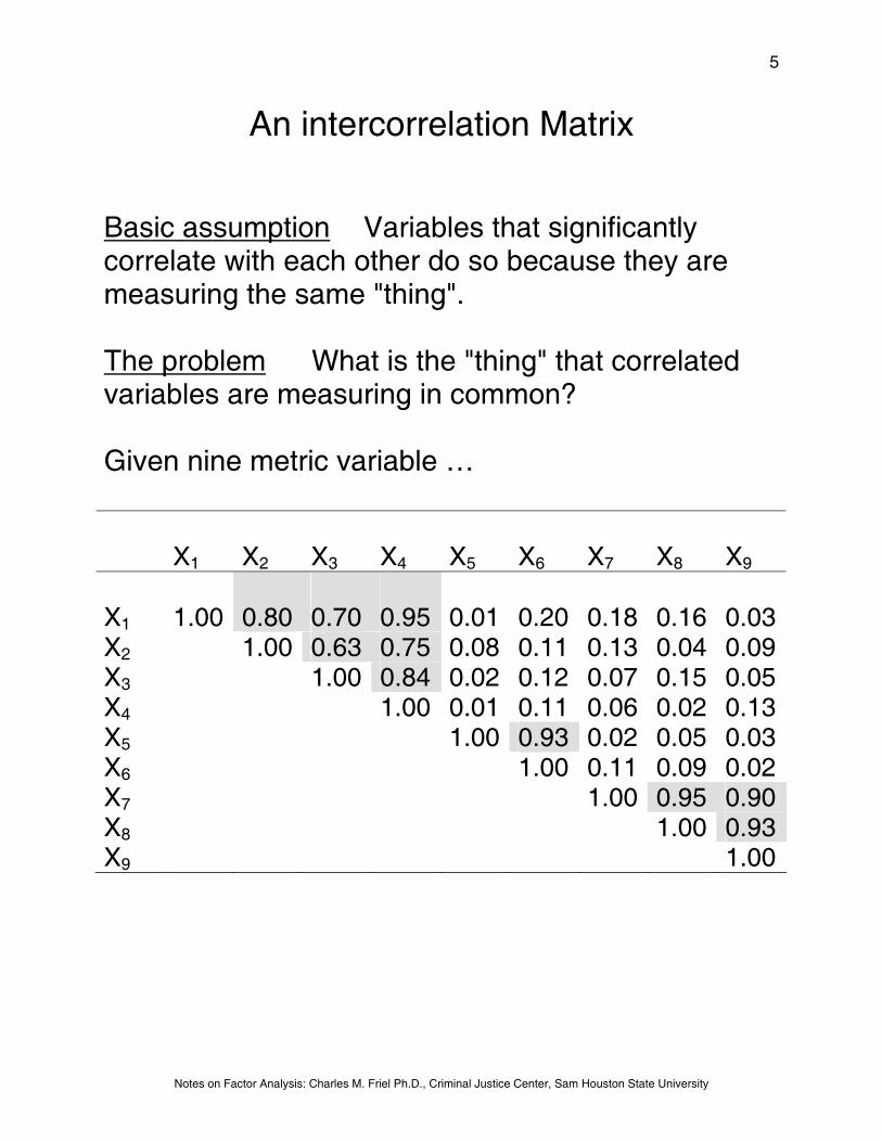
An intercorrelation Matrix Basic assumption Variables that significantly correlate with each other do so because they are measuring the same "thing". The problem What is the "thing" that correlated variables are measuring in common? Given nine metric variable …

X1 X2

X3

X4

X5

X6

X7

X8

X9

X1

1.00

0.80

0.70

0.95

0.01

0.20

0.18

0.16

0.03

X2 1.00 0.63 0.75 0.08 0.11 0.13 0.04 0.09 X3 1.00 0.84 0.02 0.12 0.07 0.15 0.05 X4 1.00 0.01 0.11 0.06 0.02 0.13 X5 1.00 0.93 0.02 0.05 0.03 X6 1.00 0.11 0.09 0.02 X7 1.00 0.95 0.90 X8 1.00 0.93 X9 1.00


6

An intercorrelation Matrix (cont.)

Notice the patterns of intercorrelation

Variables 1, 2, 3 & 4 correlate highly with each other, but not with the rest of the variables

Variables 5 & 6 correlate highly with each other, but not with the rest of the variables

Variables 7, 8, & 9 correlate highly with each other, but not with the rest of the variables

Deduction The nine variables seem to be measuring 3 "things" or underlying factors. Q What are these three factors?

Q To what extent does each variable measure each of these three factors?


7

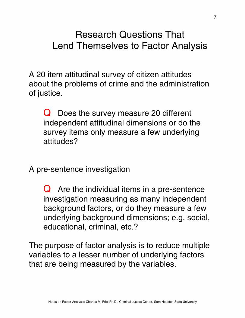
Research Questions That Lend Themselves to Factor Analysis

A 20 item attitudinal survey of citizen attitudes about the problems of crime and the administration of justice.

Q Does the survey measure 20 different independent attitudinal dimensions or do the survey items only measure a few underlying attitudes?

A pre-sentence investigation

Q Are the individual items in a pre-sentence investigation measuring as many independent background factors, or do they measure a few underlying background dimensions; e.g. social, educational, criminal, etc.?

The purpose of factor analysis is to reduce multiple variables to a lesser number of underlying factors that are being measured by the variables.


8

Applications of Factor Analysis Exploratory factor analysis A non-theoretical application. Given a set of variables, what are the underlying dimensions (factors), if any, that account for the patterns of collinearity among the variables?

Example Given the multiple items of information gathered on applicants applying for admission to a police academy, how many independent factors are actually being measured by these items?

Confirmatory factor analysis Given a theory with four concepts that purport to explain some behavior, do multiple measures of the behavior reduce to these four factors?

Example Given a theory that attributes delinquency to four independent factors, do multiple measures on delinquents reduce to measuring these four factors?


9

Applications of Factor Analysis (cont.)

R and Q Factor Analysis

R factor analysis involves extracting latent factors from among the variables

Q factor analysis involves factoring the subjects vis-à-vis the variables. The result is a "clustering" of the subjects into independent groups based upon factors extracted from the data.

This application is not used much today since a variety of clustering techniques have been developed that are designed specifically for the purpose of grouping multiple subjects into independent groups.


10

The Logic of Factor Analysis Given an N by k database …

Subjects

Variables

X1 X2 X3 … Xk 1 2 12 0 … 113 2 5 16 2 … 116 3 7 8 1 … 214 … … … … … … N 12 23 0 … 168 Compute a k x k intercorrelation matrix …

X1 X2 X3 … Xk X1 1.00 0.26 0.84 … 0.72 X2 1.00 0.54 … 0.63 X3 1.00 … 0.47 … … … Xk 1.00

Reduce the intercorrelation matrix to a k x F matrix of factor loadings … +

Variables Factor I Factor II Factor III X1 0.932 0.013 0.250 X2 0.851 0.426 0.211 X3 0.134 0.651 0.231 … … … 0.293 Xk 0.725 0.344 0.293


11

What is a Factor Loading? A factor loading is the correlation between a variable and a factor that has been extracted from the data. Example Note the factor loadings for variable X1.

Variables Factor I Factor II Factor III X1 0.932 0.013 0.250

Interpretation

Variable X1 is highly correlated with Factor I, but negligibly correlated with Factors II and III

Q How much of the variance in variable X1 is measured or accounted for by the three factors that were extracted?

Simply square the factor loadings and add them together (0.9322 + 0.0132 + 0.2502) = 0.93129 This is called the communality of the variable.


12

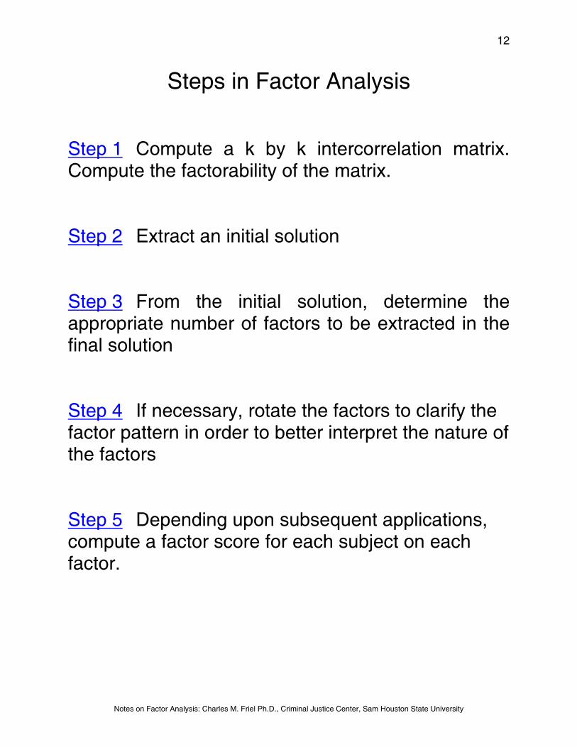
Steps in Factor Analysis Step 1 Compute a k by k intercorrelation matrix. Compute the factorability of the matrix. Step 2 Extract an initial solution Step 3 From the initial solution, determine the appropriate number of factors to be extracted in the final solution Step 4 If necessary, rotate the factors to clarify the factor pattern in order to better interpret the nature of the factors Step 5 Depending upon subsequent applications, compute a factor score for each subject on each factor.


13

An Eleven Variable Example The variables and their code names • Sentence (sentence)

• Number of prior convictions(pr_conv)

• Intelligence (iq)

• Drug dependency (dr_score)

• Chronological age (age)

• Age at 1st arrest (age_firs)

• Time to case disposition (tm_disp)

• Pre-trial jail time (jail_tm)

• Time served on sentence (tm_serv)

• Educational equivalency (educ_eqv)

• Level of work skill (skl_indx)


14

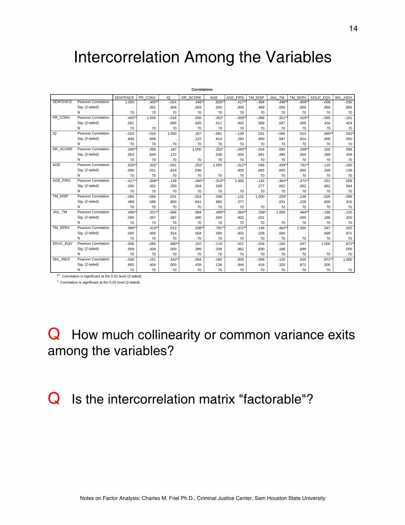
Intercorrelation Among the Variables

Correlations

1.000 .400** -.024 .346** .826** -.417** -.084 .496** .969** -.006 -.030. .001 .846 .003 .000 .000 .489 .000 .000 .959 .805

70 70 70 70 70 70 70 70 70 70 70.400** 1.000 -.016 .056 .302* -.358** -.066 .321** .419** -.095 -.101.001 . .895 .645 .011 .002 .589 .007 .000 .434 .404

70 70 70 70 70 70 70 70 70 70 70-.024 -.016 1.000 .187 -.061 -.139 .031 -.066 .013 .680** .542**.846 .895 . .122 .614 .250 .800 .587 .914 .000 .000

70 70 70 70 70 70 70 70 70 70 70.346** .056 .187 1.000 .252* -.340** -.024 .084 .338** .102 .094.003 .645 .122 . .036 .004 .841 .490 .004 .399 .439

70 70 70 70 70 70 70 70 70 70 70.826** .302* -.061 .252* 1.000 -.312** .048 .499** .781** -.116 -.180.000 .011 .614 .036 . .009 .692 .000 .000 .339 .136

70 70 70 70 70 70 70 70 70 70 70-.417** -.358** -.139 -.340** -.312** 1.000 -.132 -.364** -.372** .021 .009.000 .002 .250 .004 .009 . .277 .002 .002 .862 .944

70 70 70 70 70 70 70 70 70 70 70-.084 -.066 .031 -.024 .048 -.132 1.000 .258* -.146 -.026 -.099.489 .589 .800 .841 .692 .277 . .031 .228 .830 .416

70 70 70 70 70 70 70 70 70 70 70.496** .321** -.066 .084 .499** -.364** .258* 1.000 .464** -.160 -.120.000 .007 .587 .490 .000 .002 .031 . .000 .186 .320

70 70 70 70 70 70 70 70 70 70 70.969** .419** .013 .338** .781** -.372** -.146 .464** 1.000 .047 .020.000 .000 .914 .004 .000 .002 .228 .000 . .699 .871

70 70 70 70 70 70 70 70 70 70 70-.006 -.095 .680** .102 -.116 .021 -.026 -.160 .047 1.000 .872**.959 .434 .000 .399 .339 .862 .830 .186 .699 . .000

70 70 70 70 70 70 70 70 70 70 70-.030 -.101 .542** .094 -.180 .009 -.099 -.120 .020 .872** 1.000.805 .404 .000 .439 .136 .944 .416 .320 .871 .000 .

70 70 70 70 70 70 70 70 70 70 70

Pearson CorrelationSig. (2-tailed)NPearson CorrelationSig. (2-tailed)NPearson CorrelationSig. (2-tailed)NPearson CorrelationSig. (2-tailed)NPearson CorrelationSig. (2-tailed)NPearson CorrelationSig. (2-tailed)NPearson CorrelationSig. (2-tailed)NPearson CorrelationSig. (2-tailed)NPearson CorrelationSig. (2-tailed)NPearson CorrelationSig. (2-tailed)NPearson CorrelationSig. (2-tailed)N

SENTENCE

PR_CONV

IQ

DR_SCORE

AGE

AGE_FIRS

TM_DISP

JAIL_TM

TM_SERV

EDUC_EQV

SKL_INDX

SENTENCE PR_CONV IQ DR_SCORE AGE AGE_FIRS TM_DISP JAIL_TM TM_SERV EDUC_EQV SKL_INDX

Correlation is significant at the 0.01 level (2-tailed).**.

Correlation is significant at the 0.05 level (2-tailed).*. Q How much collinearity or common variance exits among the variables? Q Is the intercorrelation matrix "factorable"?


15

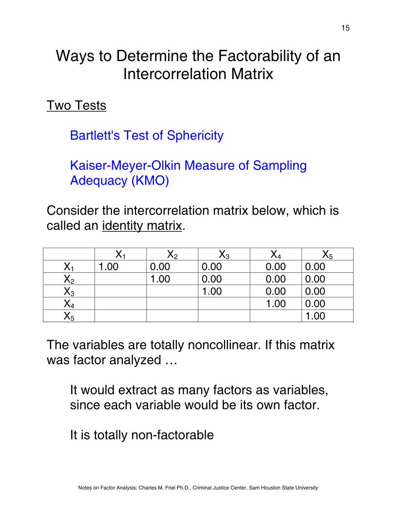
Ways to Determine the Factorability of an Intercorrelation Matrix

Two Tests Bartlett's Test of Sphericity

Kaiser-Meyer-Olkin Measure of Sampling Adequacy (KMO)

Consider the intercorrelation matrix below, which is called an identity matrix.

X1 X2 X3 X4 X5 X1 1.00 0.00 0.00 0.00 0.00 X2 1.00 0.00 0.00 0.00 X3 1.00 0.00 0.00 X4 1.00 0.00 X5 1.00

The variables are totally noncollinear. If this matrix was factor analyzed …

It would extract as many factors as variables, since each variable would be its own factor. It is totally non-factorable


16

Bartlett's Test of Sphericity In matrix algebra, the determinate of an identity matrix is equal to 1.0. For example … 1.0 0.0 I = 0.0 1.0 1.0 0.0 I = 0.0 1.0 I = (1.0 x 1.0) - (0.0 x 0.0) = 1.0 Example Given the intercorrelation matrix below, what is its determinate? 1.0 0.63 R =

0.63 1.00

R = (1.0 x 1.0) - (0.63 x 0.63) = 0.6031


17

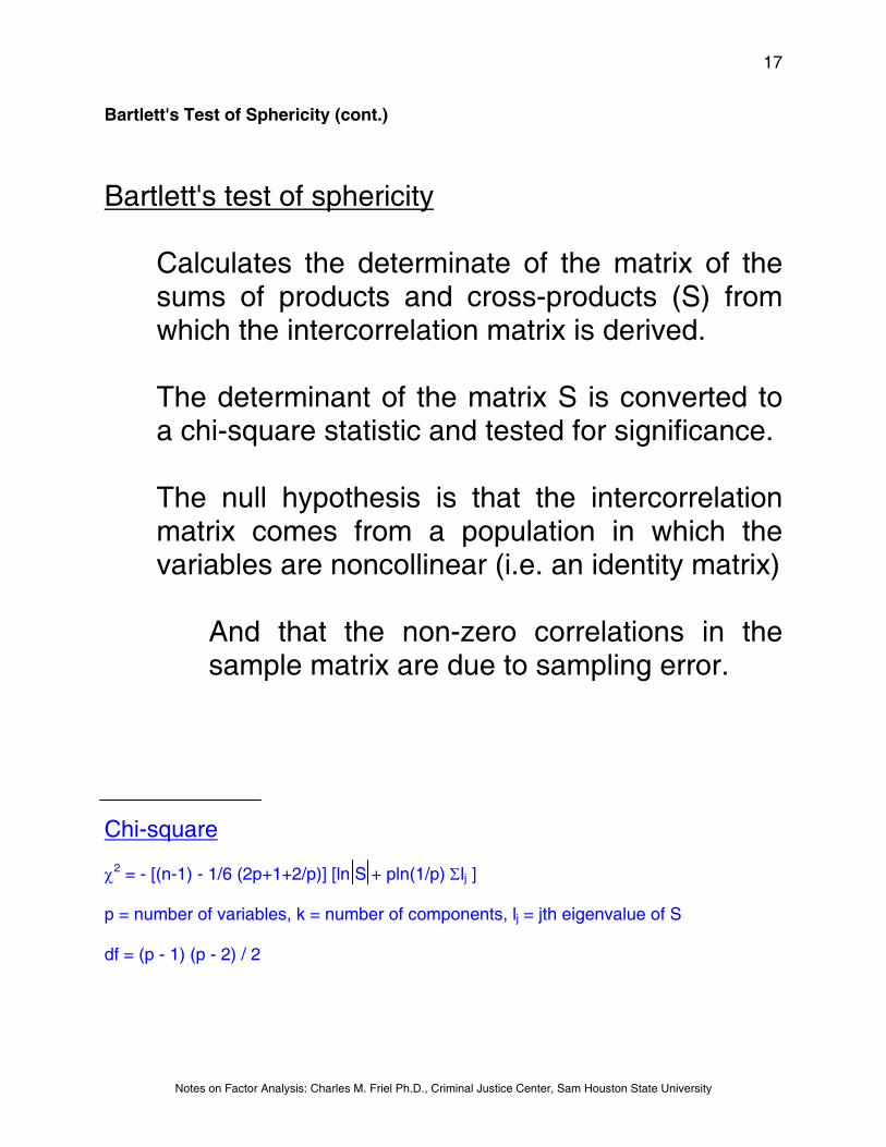
Bartlett's Test of Sphericity (cont.)

Bartlett's test of sphericity

Calculates the determinate of the matrix of the sums of products and cross-products (S) from which the intercorrelation matrix is derived. The determinant of the matrix S is converted to a chi-square statistic and tested for significance. The null hypothesis is that the intercorrelation matrix comes from a population in which the variables are noncollinear (i.e. an identity matrix)

And that the non-zero correlations in the sample matrix are due to sampling error.

Chi-square χ2 = - [(n-1) - 1/6 (2p+1+2/p)] [ln S + pln(1/p) Σlj ] p = number of variables, k = number of components, lj = jth eigenvalue of S df = (p - 1) (p - 2) / 2


18

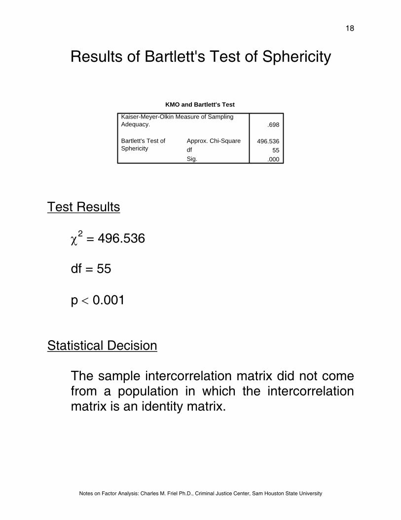
Results of Bartlett's Test of Sphericity

KMO and Bartlett's Test

.698

496.53655

.000

Kaiser-Meyer-Olkin Measure of SamplingAdequacy.

Approx. Chi-SquaredfSig.

Bartlett's Test ofSphericity

Test Results χ2 = 496.536 df = 55 p < 0.001 Statistical Decision

The sample intercorrelation matrix did not come from a population in which the intercorrelation matrix is an identity matrix.


19

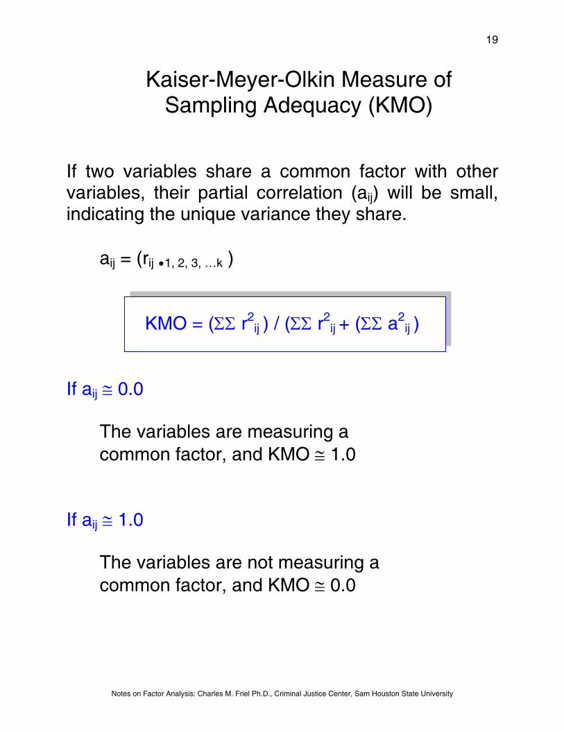
Kaiser-Meyer-Olkin Measure of Sampling Adequacy (KMO)

If two variables share a common factor with other variables, their partial correlation (aij) will be small, indicating the unique variance they share.

aij = (rij •1, 2, 3, …k )

KMO = (ΣΣ r2ij ) / (ΣΣ r2

ij + (ΣΣ a2ij )

If aij ≅ 0.0

The variables are measuring a common factor, and KMO ≅ 1.0

If aij ≅ 1.0

The variables are not measuring a common factor, and KMO ≅ 0.0


20

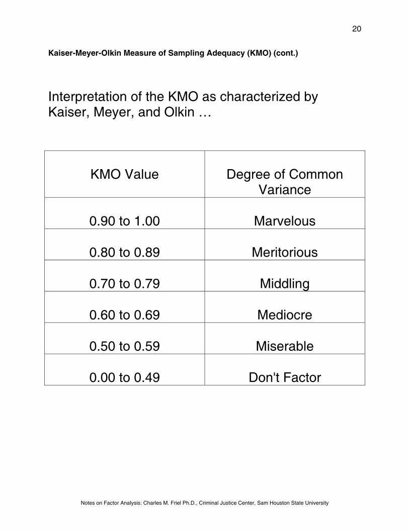
Kaiser-Meyer-Olkin Measure of Sampling Adequacy (KMO) (cont.)

Interpretation of the KMO as characterized by Kaiser, Meyer, and Olkin …

KMO Value

Degree of Common

Variance

0.90 to 1.00

Marvelous

0.80 to 0.89

Meritorious

0.70 to 0.79

Middling

0.60 to 0.69

Mediocre

0.50 to 0.59

Miserable

0.00 to 0.49

Don't Factor


21

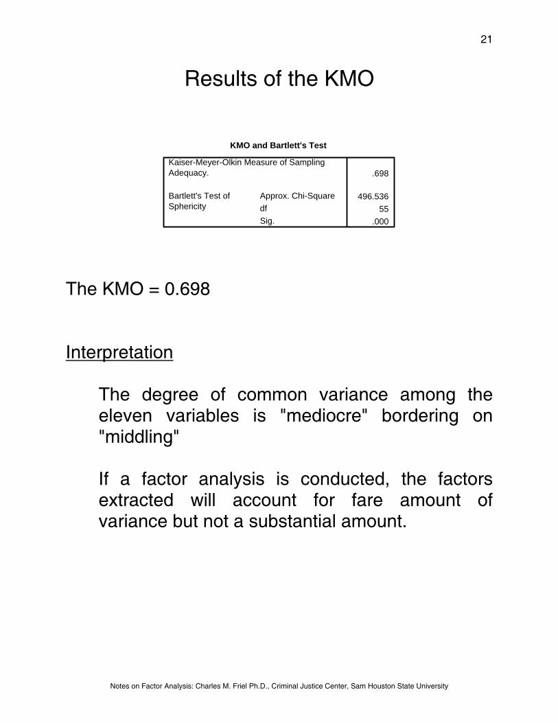
Results of the KMO

KMO and Bartlett's Test

.698

496.53655

.000

Kaiser-Meyer-Olkin Measure of SamplingAdequacy.

Approx. Chi-SquaredfSig.

Bartlett's Test ofSphericity

The KMO = 0.698 Interpretation

The degree of common variance among the eleven variables is "mediocre" bordering on "middling" If a factor analysis is conducted, the factors extracted will account for fare amount of variance but not a substantial amount.


22

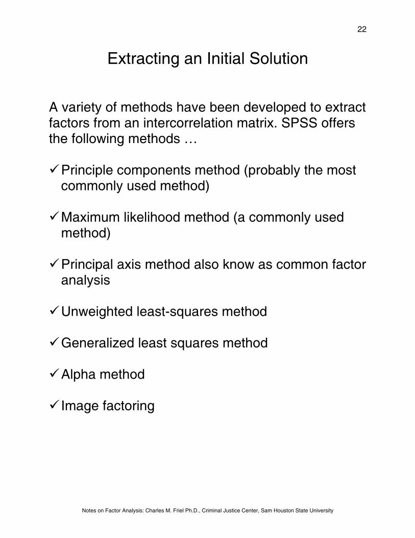
Extracting an Initial Solution A variety of methods have been developed to extract factors from an intercorrelation matrix. SPSS offers the following methods …

Principle components method (probably the most commonly used method)

Maximum likelihood method (a commonly used method)

Principal axis method also know as common factor analysis

Unweighted least-squares method

Generalized least squares method

Alpha method

Image factoring


23

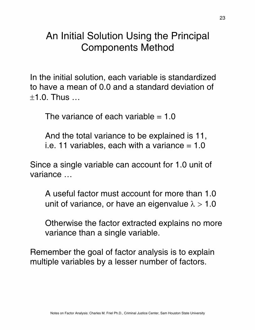
An Initial Solution Using the Principal Components Method

In the initial solution, each variable is standardized to have a mean of 0.0 and a standard deviation of ±1.0. Thus … The variance of each variable = 1.0 And the total variance to be explained is 11, i.e. 11 variables, each with a variance = 1.0 Since a single variable can account for 1.0 unit of variance …

A useful factor must account for more than 1.0 unit of variance, or have an eigenvalue λ > 1.0 Otherwise the factor extracted explains no more variance than a single variable.

Remember the goal of factor analysis is to explain multiple variables by a lesser number of factors.


24

The Results of the Initial Solution

Total Variance Explained

3.698 33.617 33.617 3.698 33.617 33.6172.484 22.580 56.197 2.484 22.580 56.1971.237 11.242 67.439 1.237 11.242 67.439

.952 8.653 76.092

.898 8.167 84.259

.511 4.649 88.908

.468 4.258 93.165

.442 4.022 97.187

.190 1.724 98.9119.538E-02 .867 99.7782.437E-02 .222 100.000

Component1234567891011

Total % of Variance Cumulative % Total % of Variance Cumulative %Initial Eigenvalues Extraction Sums of Squared Loadings

Extraction Method: Principal Component Analysis. 11 factors (components) were extracted, the same as the number of variables factored. Factor I The 1st factor has an eigenvalue = 3.698. Since this is greater than 1.0, it explains more variance than a single variable, in fact 3.698 times as much.

The percent a variance explained … (3.698 / 11 units of variance) (100) = 33.617%


25

The Results of the Initial Solution (cont.)

Factor II The 2nd factor has an eigenvalue = 2.484. It is also greater than 1.0, and therefore explains more variance than a single variable

The percent a variance explained (2.484 / 11 units of variance) (100) = 22.580% Factor III The 3rd factor has an eigenvalue = 1.237. Like Factors I & II it is greater than 1.0, and therefore explains more variance than a single variable.

The percent a variance explained (1.237 / 11 units of variance) (100) = 11.242% The remaining factors

Factors 4 through 11 have eigenvalues less that 1, and therefore explain less variance that a single variable.


26

The Results of the Initial Solution (cont.)

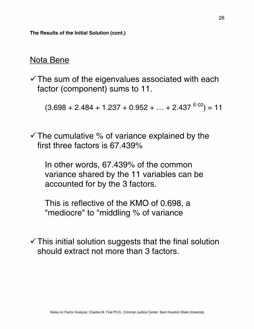
Nota Bene

The sum of the eigenvalues associated with each factor (component) sums to 11.

(3.698 + 2.484 + 1.237 + 0.952 + … + 2.437 E-02) = 11

The cumulative % of variance explained by the first three factors is 67.439%

In other words, 67.439% of the common variance shared by the 11 variables can be accounted for by the 3 factors.

This is reflective of the KMO of 0.698, a "mediocre" to "middling % of variance

This initial solution suggests that the final solution should extract not more than 3 factors.


27

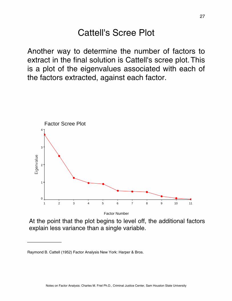
Cattell's Scree Plot Another way to determine the number of factors to extract in the final solution is Cattell's scree plot. This is a plot of the eigenvalues associated with each of the factors extracted, against each factor.

At the point that the plot begins to level off, the additional factors explain less variance than a single variable.

Raymond B. Cattell (1952) Factor Analysis New York: Harper & Bros.

Factor Scree Plot

1110987654321

4

3

2

1

0

Factor Number


28

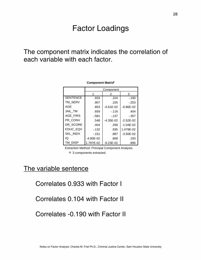
Factor Loadings The component matrix indicates the correlation of each variable with each factor.

Component Matrixa

.933 .104 -.190

.907 .155 -.253

.853 -4.61E-02 -6.86E-02

.659 -.116 .404-.581 -.137 -.357.548 -4.35E-02 -2.52E-02.404 .299 -1.04E-02

-.132 .935 1.479E-02-.151 .887 -3.50E-02

-4.80E-02 .808 .1931.787E-02 -9.23E-02 .896

SENTENCETM_SERVAGEJAIL_TMAGE_FIRSPR_CONVDR_SCOREEDUC_EQVSKL_INDXIQTM_DISP

1 2 3Component

Extraction Method: Principal Component Analysis.3 components extracted.a.

The variable sentence Correlates 0.933 with Factor I Correlates 0.104 with Factor II Correlates -0.190 with Factor II


29

Factor Loadings (cont.)

The total proportion of the variance in sentence explained by the three factors is simply the sum of its squared factor loadings. (0.9332 + 0.1042 - 0.1902) = 0.917

This is called the communality of the variable sentence

The communalities of the 11 variables are as follows: (cf. column headed Extraction)

Communalities

1.000 .9171.000 .3031.000 .6931.000 .2521.000 .8111.000 .6111.000 .9101.000 .8931.000 .8111.000 .7351.000 .483

SENTENCEPR_CONVIQDR_SCORETM_DISPJAIL_TMTM_SERVEDUC_EQVSKL_INDXAGEAGE_FIRS

Initial Extraction

Extraction Method: Principal Component Analysis.

As is evident from the table, the proportion of variance in each variable accounted for by the three factors is not the same.


30

What Do the Three Factors Measure? The key to determining what the factors measure is the factor loadings For example

Which variables load (correlate) highest on Factor I and low on the other two factors?

Component Matrixa

.933 .104 -.190

.907 .155 -.253

.853 -4.61E-02 -6.86E-02

.659 -.116 .404-.581 -.137 -.357.548 -4.35E-02 -2.52E-02.404 .299 -1.04E-02

-.132 .935 1.479E-02-.151 .887 -3.50E-02

-4.80E-02 .808 .1931.787E-02 -9.23E-02 .896

SENTENCETM_SERVAGEJAIL_TMAGE_FIRSPR_CONVDR_SCOREEDUC_EQVSKL_INDXIQTM_DISP

1 2 3Component


Factor I

sentence (.933) tm_serv (.907) age (.853) jail_tm (.659) age_firs (-.581) pr_conv (.548) dr_score (.404)


31

What Do the Three Factors Measure? (cont.)

Naming Factor I What do these seven variables have in common, particularly the first few that have the highest loading on Factor I?

Degree of criminality? Career criminal history? You name it …

Factor II

educ_equ (.935) skl_indx (.887) iq (.808)

Naming Factor II Educational level or job skill level? Factor III

Tm_disp (.896)

Naming Factor III This factor is difficult to understand since only one variable loaded highest on it. Could this be a measure of criminal case processing dynamics? We would need more variables loading on this factor to know.


32

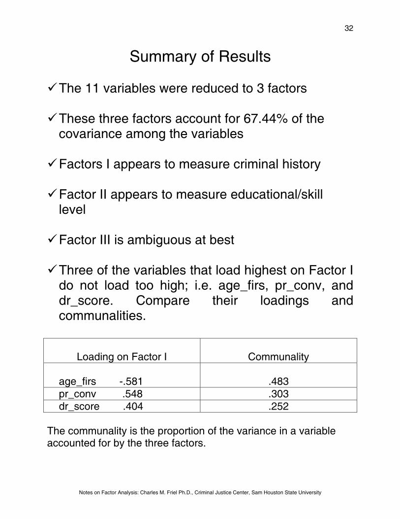
Summary of Results

The 11 variables were reduced to 3 factors

These three factors account for 67.44% of the covariance among the variables

Factors I appears to measure criminal history

Factor II appears to measure educational/skill level

Factor III is ambiguous at best

Three of the variables that load highest on Factor I do not load too high; i.e. age_firs, pr_conv, and dr_score. Compare their loadings and communalities.

Loading on Factor I

Communality age_firs -.581

.483

pr_conv .548 .303 dr_score .404 .252

The communality is the proportion of the variance in a variable accounted for by the three factors.


33

What Can Be Done if the Factor Pattern Is Not Clear?

Sometimes one or more variables may load about the same on more than one factor, making the interpretation of the factors ambiguous. Ideally, the analyst would like to find that each variable loads high (⇒ 1.0) on one factor and approximately zero on all the others (⇒ 0.0).

An Ideal Component Matrix

Variables Factors (f) I II … f

X1 1.0 0.0 … 0.0 X2 1.0 0.0 … 0.0 X3 0.0 0.0 … 1.0 X4 0.0 1.0 … 0.0 … … … … … Xk 0.0 0.0 … 1.0

The values in the matrix are factor loadings, the correlations between each variable and each factor.


34

Factor Rotation Sometimes the factor pattern can be clarified by "rotating" the factors in F-dimensional space. Consider the following hypothetical two-factor solution involving eight variables. F I X8 X1 X4 X6 F II X3 X5 X7 X2 Variables 1 & 2 load on Factor I, while variables 3, 5, & 6 load on Factor II. Variables 4, 7, & 8 load about the same on both factors. What happens if the axes are rotated?


35

Factor Rotation (cont.)

Orthogonal rotation The axes remain 90° apart F I X8 X1 X4 X6 F II X3 X5 X7 X2 Variables 1, 2, 5, 7, & 8 load on Factor II, while variables 3, 4, & 6 load on Factor I. Notice that relative to variables 4, 7, & 8, the rotated factor pattern is clearer than the previously unrotated pattern.


36

What Criterion is Used in Factor Rotation? There are various methods that can be used in factor rotation … Varimax Rotation

Attempts to achieve loadings of ones and zeros in the columns of the component matrix (1.0 & 0.0).

Quartimax Rotation

Attempts to achieve loadings of ones and zeros in the rows of the component matrix (1.0 & 0.0).

Equimax Rotation

Combines the objectives of both varimax and quartimax rotations

Orthogonal Rotation

Preserves the independence of the factors, geometrically they remain 90° apart.

Oblique Rotation

Will produce factors that are not independent, geometrically not 90° apart.


37

Rotation of the Eleven Variable Case Study Method Varimax rotation. Below are the unrotated and rotated component matrices.

Component Matrixa

.933 .104 -.190

.548 -4.35E-02 -2.52E-02-4.80E-02 .808 .193

.404 .299 -1.04E-021.787E-02 -9.23E-02 .896

.659 -.116 .404

.907 .155 -.253-.132 .935 1.479E-02-.151 .887 -3.50E-02.853 -4.61E-02 -6.86E-02

-.581 -.137 -.357


1 2 3Component


Rotated Component Matrixa

.956 -2.59E-03 -5.62E-02

.539 -9.79E-02 5.956E-021.225E-02 .823 .128

.431 .257 2.933E-02-.118 -1.88E-02 .892.579 -.145 .504.945 4.563E-02 -.126

-3.15E-02 .942 -6.89E-02-4.89E-02 .891 -.118

.844 -.133 6.221E-02-.536 -.110 -.429


1 2 3Component

Extraction Method: Principal Component Analysis. Rotation Method: Varimax with Kaiser Normalization.

Rotation converged in 4 iterations.a.


38

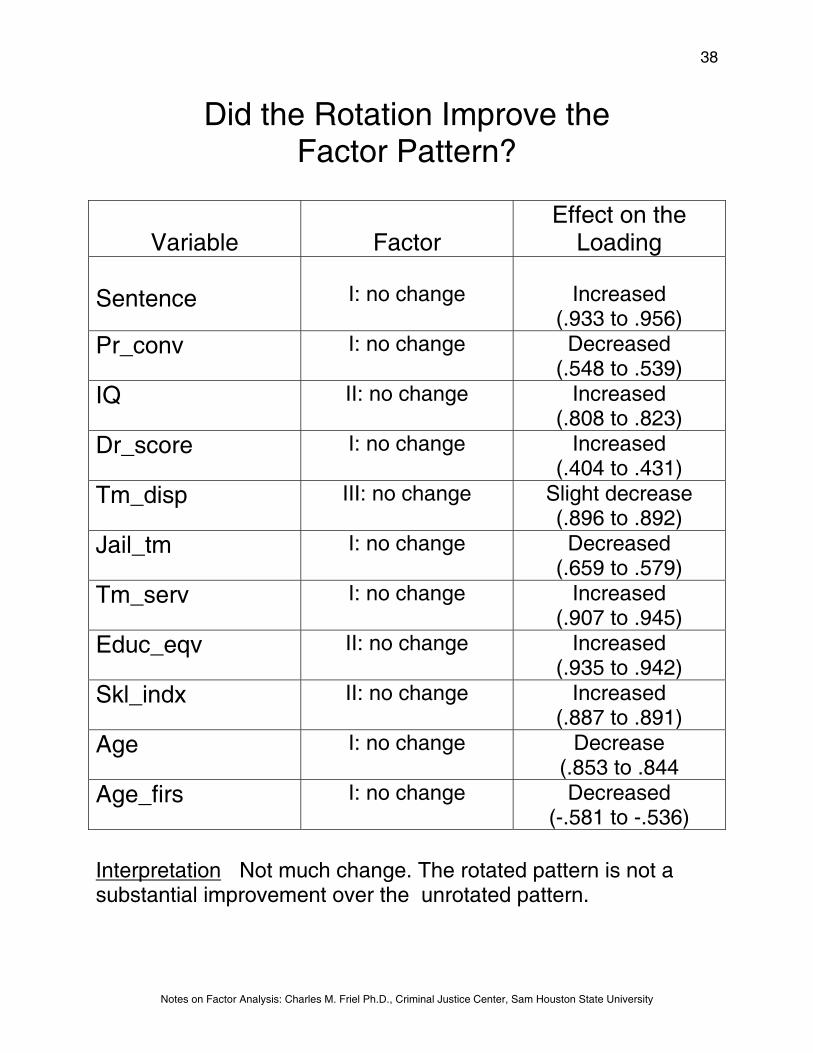
Did the Rotation Improve the Factor Pattern?

Variable

Factor Effect on the

Loading Sentence

I: no change

Increased

(.933 to .956) Pr_conv I: no change Decreased

(.548 to .539) IQ II: no change Increased

(.808 to .823) Dr_score I: no change Increased

(.404 to .431) Tm_disp III: no change Slight decrease

(.896 to .892) Jail_tm I: no change Decreased

(.659 to .579) Tm_serv I: no change Increased

(.907 to .945) Educ_eqv II: no change Increased

(.935 to .942) Skl_indx II: no change Increased

(.887 to .891) Age I: no change Decrease

(.853 to .844 Age_firs I: no change Decreased

(-.581 to -.536) Interpretation Not much change. The rotated pattern is not a substantial improvement over the unrotated pattern.


39

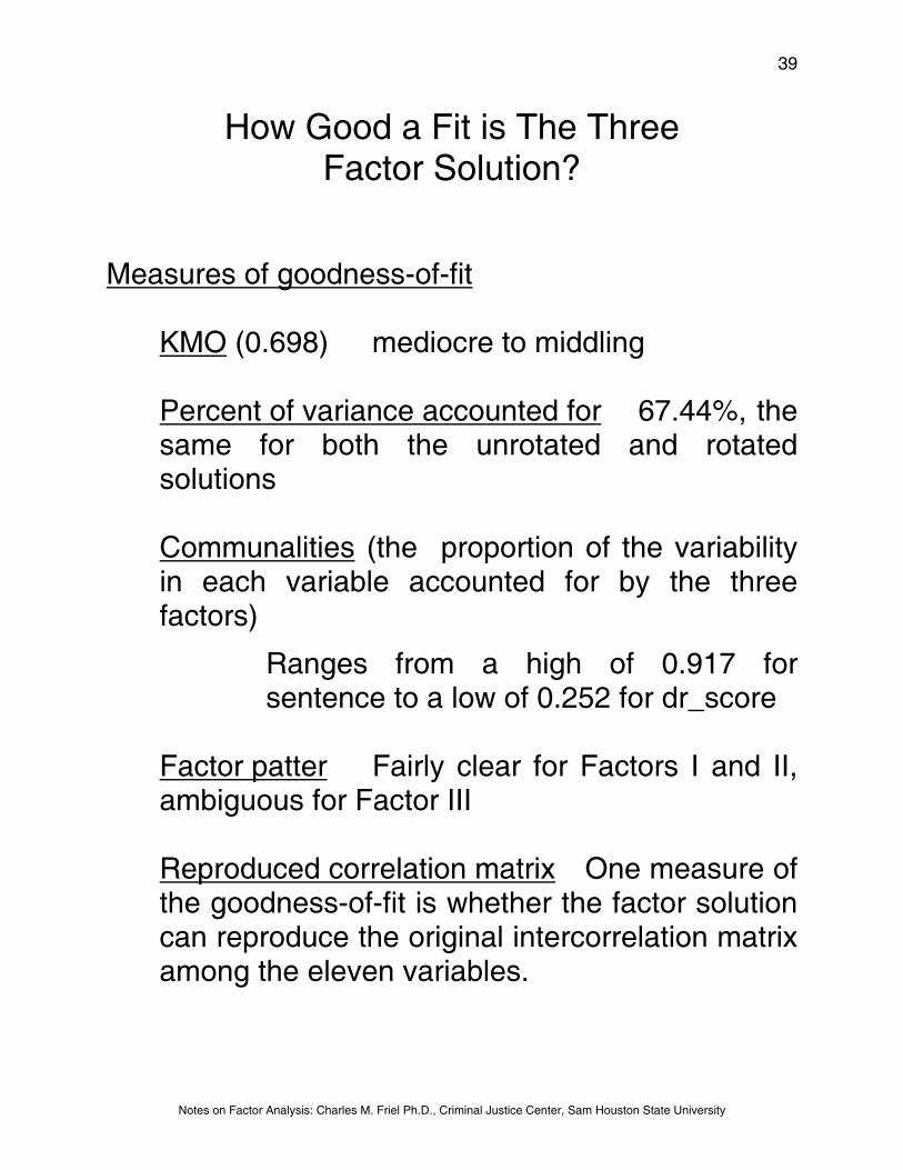
How Good a Fit is The Three Factor Solution?

Measures of goodness-of-fit KMO (0.698) mediocre to middling

Percent of variance accounted for 67.44%, the same for both the unrotated and rotated solutions Communalities (the proportion of the variability in each variable accounted for by the three factors)

Ranges from a high of 0.917 for sentence to a low of 0.252 for dr_score

Factor patter Fairly clear for Factors I and II, ambiguous for Factor III Reproduced correlation matrix One measure of the goodness-of-fit is whether the factor solution can reproduce the original intercorrelation matrix among the eleven variables.


40

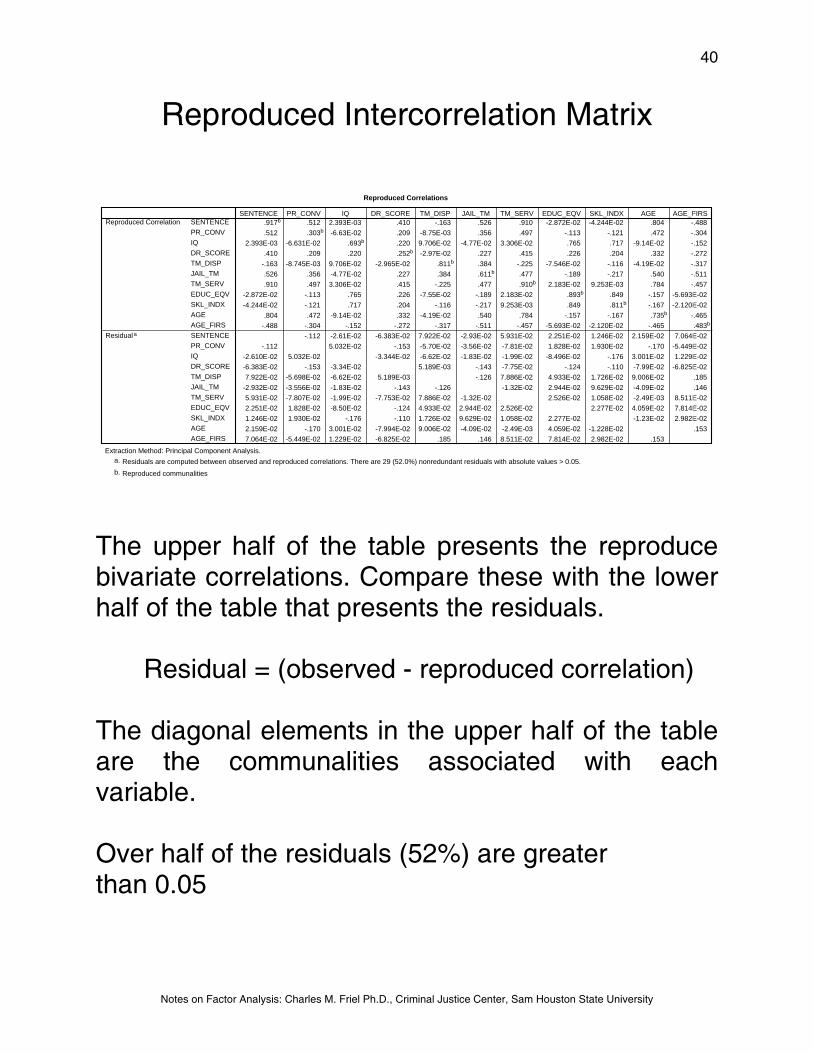
Reproduced Intercorrelation Matrix

Reproduced Correlations

.917b .512 2.393E-03 .410 -.163 .526 .910 -2.872E-02 -4.244E-02 .804 -.488

.512 .303b -6.63E-02 .209 -8.75E-03 .356 .497 -.113 -.121 .472 -.3042.393E-03 -6.631E-02 .693b .220 9.706E-02 -4.77E-02 3.306E-02 .765 .717 -9.14E-02 -.152

.410 .209 .220 .252b -2.97E-02 .227 .415 .226 .204 .332 -.272-.163 -8.745E-03 9.706E-02 -2.965E-02 .811b .384 -.225 -7.546E-02 -.116 -4.19E-02 -.317.526 .356 -4.77E-02 .227 .384 .611b .477 -.189 -.217 .540 -.511.910 .497 3.306E-02 .415 -.225 .477 .910b 2.183E-02 9.253E-03 .784 -.457

-2.872E-02 -.113 .765 .226 -7.55E-02 -.189 2.183E-02 .893b .849 -.157 -5.693E-02-4.244E-02 -.121 .717 .204 -.116 -.217 9.253E-03 .849 .811b -.167 -2.120E-02

.804 .472 -9.14E-02 .332 -4.19E-02 .540 .784 -.157 -.167 .735b -.465-.488 -.304 -.152 -.272 -.317 -.511 -.457 -5.693E-02 -2.120E-02 -.465 .483b

-.112 -2.61E-02 -6.383E-02 7.922E-02 -2.93E-02 5.931E-02 2.251E-02 1.246E-02 2.159E-02 7.064E-02-.112 5.032E-02 -.153 -5.70E-02 -3.56E-02 -7.81E-02 1.828E-02 1.930E-02 -.170 -5.449E-02

-2.610E-02 5.032E-02 -3.344E-02 -6.62E-02 -1.83E-02 -1.99E-02 -8.496E-02 -.176 3.001E-02 1.229E-02-6.383E-02 -.153 -3.34E-02 5.189E-03 -.143 -7.75E-02 -.124 -.110 -7.99E-02 -6.825E-027.922E-02 -5.698E-02 -6.62E-02 5.189E-03 -.126 7.886E-02 4.933E-02 1.726E-02 9.006E-02 .185

-2.932E-02 -3.556E-02 -1.83E-02 -.143 -.126 -1.32E-02 2.944E-02 9.629E-02 -4.09E-02 .1465.931E-02 -7.807E-02 -1.99E-02 -7.753E-02 7.886E-02 -1.32E-02 2.526E-02 1.058E-02 -2.49E-03 8.511E-022.251E-02 1.828E-02 -8.50E-02 -.124 4.933E-02 2.944E-02 2.526E-02 2.277E-02 4.059E-02 7.814E-021.246E-02 1.930E-02 -.176 -.110 1.726E-02 9.629E-02 1.058E-02 2.277E-02 -1.23E-02 2.982E-022.159E-02 -.170 3.001E-02 -7.994E-02 9.006E-02 -4.09E-02 -2.49E-03 4.059E-02 -1.228E-02 .1537.064E-02 -5.449E-02 1.229E-02 -6.825E-02 .185 .146 8.511E-02 7.814E-02 2.982E-02 .153

SENTENCEPR_CONVIQDR_SCORETM_DISPJAIL_TMTM_SERVEDUC_EQVSKL_INDXAGEAGE_FIRSSENTENCEPR_CONVIQDR_SCORETM_DISPJAIL_TMTM_SERVEDUC_EQVSKL_INDXAGEAGE_FIRS

Reproduced Correlation

Residuala

SENTENCE PR_CONV IQ DR_SCORE TM_DISP JAIL_TM TM_SERV EDUC_EQV SKL_INDX AGE AGE_FIRS

Extraction Method: Principal Component Analysis.Residuals are computed between observed and reproduced correlations. There are 29 (52.0%) nonredundant residuals with absolute values > 0.05.a.

Reproduced communalitiesb.

The upper half of the table presents the reproduce bivariate correlations. Compare these with the lower half of the table that presents the residuals. Residual = (observed - reproduced correlation) The diagonal elements in the upper half of the table are the communalities associated with each variable. Over half of the residuals (52%) are greater than 0.05


41

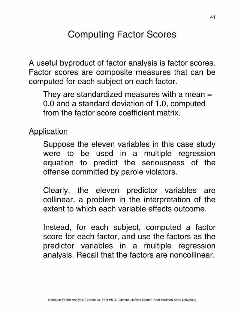
Computing Factor Scores A useful byproduct of factor analysis is factor scores. Factor scores are composite measures that can be computed for each subject on each factor.

They are standardized measures with a mean = 0.0 and a standard deviation of 1.0, computed from the factor score coefficient matrix.

Application

Suppose the eleven variables in this case study were to be used in a multiple regression equation to predict the seriousness of the offense committed by parole violators. Clearly, the eleven predictor variables are collinear, a problem in the interpretation of the extent to which each variable effects outcome. Instead, for each subject, computed a factor score for each factor, and use the factors as the predictor variables in a multiple regression analysis. Recall that the factors are noncollinear.


42

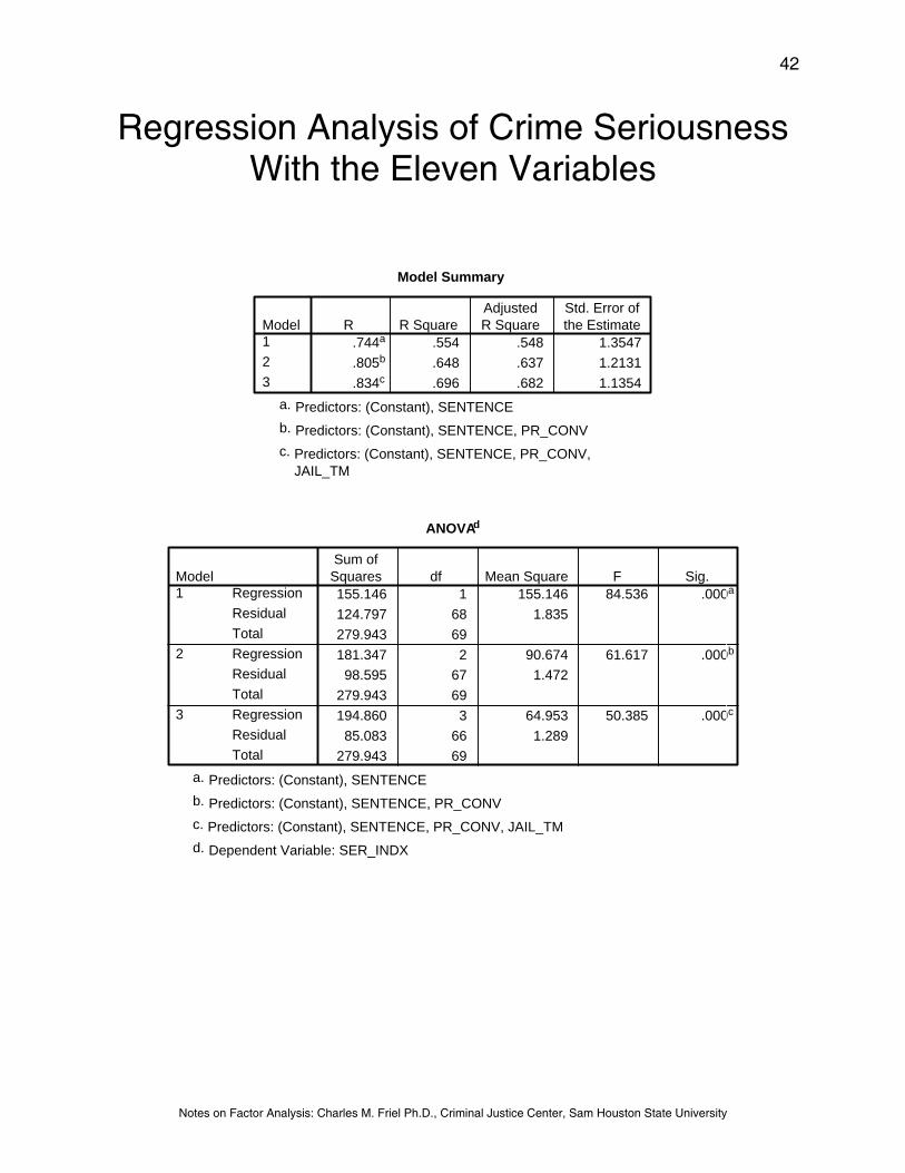
Regression Analysis of Crime Seriousness With the Eleven Variables

Model Summary

.744a .554 .548 1.3547

.805b .648 .637 1.2131

.834c .696 .682 1.1354

Model123

R R SquareAdjustedR Square

Std. Error ofthe Estimate

Predictors: (Constant), SENTENCEa.

Predictors: (Constant), SENTENCE, PR_CONVb.

Predictors: (Constant), SENTENCE, PR_CONV,JAIL_TM

c.

ANOVAd

155.146 1 155.146 84.536 .000a

124.797 68 1.835279.943 69181.347 2 90.674 61.617 .000b

98.595 67 1.472279.943 69194.860 3 64.953 50.385 .000c

85.083 66 1.289279.943 69

RegressionResidualTotalRegressionResidualTotalRegressionResidualTotal

Model1

2

3

Sum ofSquares df Mean Square F Sig.

Predictors: (Constant), SENTENCEa.

Predictors: (Constant), SENTENCE, PR_CONVb.

Predictors: (Constant), SENTENCE, PR_CONV, JAIL_TMc.

Dependent Variable: SER_INDXd.


43

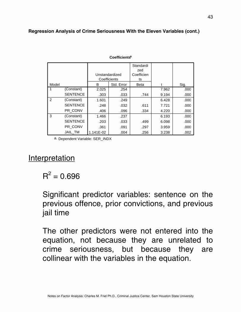
Regression Analysis of Crime Seriousness With the Eleven Variables (cont.)

Coefficientsa

2.025 .254 7.962 .000.303 .033 .744 9.194 .000

1.601 .249 6.428 .000.248 .032 .611 7.721 .000.406 .096 .334 4.220 .000

1.466 .237 6.193 .000.203 .033 .499 6.098 .000.361 .091 .297 3.959 .000

1.141E-02 .004 .256 3.238 .002

(Constant)SENTENCE(Constant)SENTENCEPR_CONV(Constant)SENTENCEPR_CONVJAIL_TM

Model1

2

3

B Std. Error

UnstandardizedCoefficients

Beta

Standardized

Coefficients

t Sig.

Dependent Variable: SER_INDXa.

Interpretation R2 = 0.696

Significant predictor variables: sentence on the previous offence, prior convictions, and previous jail time The other predictors were not entered into the equation, not because they are unrelated to crime seriousness, but because they are collinear with the variables in the equation.


44

Regression Analysis with Factor Scores

Model Summaryc

.788a .621 .615 1.2497

.802b .643 .633 1.2209

Model12

R R SquareAdjustedR Square

Std. Error ofthe Estimate

Predictors: (Constant), REGR factor score 1 foranalysis 1

a.

Predictors: (Constant), REGR factor score 1 foranalysis 1 , REGR factor score 3 for analysis 1

b.

Dependent Variable: SER_INDXc.

ANOVAc

173.747 1 173.747 111.255 .000a

106.196 68 1.562279.943 69180.081 2 90.040 60.410 .000b

99.862 67 1.490279.943 69

RegressionResidualTotalRegressionResidualTotal

Model1

2

Sum ofSquares df Mean Square F Sig.

Predictors: (Constant), REGR factor score 1 for analysis 1a.

Predictors: (Constant), REGR factor score 1 for analysis 1 , REGR factor score 3 for analysis 1

b.

Dependent Variable: SER_INDXc.

Coefficientsa

3.829 .149 25.632 .000

1.587 .150 .788 10.548 .000

3.829 .146 26.238 .000

1.587 .147 .788 10.797 .000

.303 .147 .150 2.061 .043

(Constant)REGR factor score1 for analysis 1(Constant)REGR factor score1 for analysis 1REGR factor score3 for analysis 1

Model1

2

B Std. Error

UnstandardizedCoefficients

Beta

Standardized

Coefficients

t Sig.

Dependent Variable: SER_INDXa.


45

Interpretation of the Regression Analysis With Factor Scores

R2 = 0.643 (previous regression model = 0.696) ser_indx = 3.829 + 1.587 (F I) + 0.303 (F III)

F = Factor Factors I and III were found to be significant predictors. Factor II was not significant. Factor I is assumed to be a latent factor that measures criminal history, while Factor II appears to measure educational/skill level. Since only one variable (tm_disp) loaded on Factor III, it is difficult to theorize about the nature of the latent variable it measures other than it measures time to disposition. Comparison of the beta weights indicates that the criminal history factor (Factor I) has a greater effect in explaining the seriousness of the offense than does Factor III (tm_disp).

factor analysis - university of alabama

Documents