factor scores, structure and communality coefficients: a ... scores, structure and communality...

Factor Scores 1

Running head: FACTOR SCORES

Factor scores, structure and communality coefficients: A primer

Mary Odum

Texas A&M University

Paper presented at the annual meeting of the Southwest Educational Research Association, San

Antonio, February 3, 2011.

Factor Scores 2

Abstract

This paper is an easy-to-understand primer on three important concepts of factor analysis: Factor

scores, structure coefficients, and communality coefficients. An introductory overview of

meanings and applications of each is presented. Additionally, four methods for calculating factor

scores are compared: (1) The Anderson-Rubin method (Anderson & Rubin, 1956); (2) the Bartlett

method (Bartlett, 1937); (3) the regression method (Gorsuch, 1983); and (4) the Thompson method

(Thompson, 1993). Step-by-step instructions are provided for utilizing these four methods, with

heuristic examples.

Factor Scores 3

Factor scores, structure and communality coefficients: A primer

Factor scores, structure coefficients, and communality coefficients are integral to the

interpretation and reporting of factor analytic research results. Therefore, a foundational

understanding of these three concepts is useful for students and researchers. This easy-to-follow

primer is intended to provide an introductory overview of factor scores, structure and

communality coefficients with a heuristic example using real world data from the 1939

Holzinger and Swineford data set.

An introductory overview of meanings and applications of factor scores, structure

coefficients, and communality coefficients is presented. Additionally, four methods for calculating

factor scores are compared: (1) The Anderson-Rubin method (Anderson & Rubin, 1956); (2) the

Bartlett method (Bartlett, 1937); (3) the regression method (Gorsuch, 1983); and (4) the Thompson

method (Thompson, 1993). Step-by-step instructions are provided for utilizing these four methods,

with heuristic examples utilizing publically-accessible data and the commonly used statistical

program SPSS. Interested readers may opt to follow these examples and on their own to enhance

the learning of the presented concepts (full syntax for all examples in Appendix).

After thoughtful review of this paper, readers should gain an introductory understanding of

the purposes of factor scores, structure coefficients, and communality coefficients in factor

analyses, and how to utilize SPSS for conducting various factor score estimation methods in a

factor analysis. Given that statistical analyses are a part of a global general linear model (GLM),

and utilize weights as an integral part of analyses (Thompson, 2006; Thompson, 2004),

terminology used for factor analytic procedures are analogous to terminology in other GLM

analyses. Therefore, transfer of ideas across various GLM analyses is anticipated.

Factor Scores 4

Heuristic Data

The Holzinger and Swineford (1939) data set will be used to illustrate computations and

aid discussion of factor analytic statistics. For heuristic purposes, all scores for the 301 original

participants on six of the original twenty-five measured variables will be used: “t14” – Memory

of Target Words; “t15” – Memory of Target Numbers; “t16” – Memory of Target Shapes; “t20”

– Deductive Math Ability; “t21” – Math Number Puzzles; and, “t22” – Math Word Problem

Reasoning. There seems to be two general categories that these six variables may naturally fall

into: (1) Memory; and, (2) Math ability. It would not be unreasonable, therefore, to expect to find

two factors for our six variables. A factor analysis will confirm or contradict this educated guess.

Factor Analytic Statistics

Terminology for statistical techniques can be confusing and cumbersome, especially for

those with limited statistical backgrounds. Here, relevant terms will be introduced, defined, and

presented with relevant SPSS syntax and outputs using the aforementioned six variables.

Pattern Coefficients

Pattern coefficients are weights applied to measured variables to obtain scores on latent

variables (sometimes called composite or synthetic variables) and are analogous to beta weights in

the regression equation, the set of weights for the predictors in regression analyses (Thompson,

2004). In all GLM analyses (including factor analysis), “weights [here, pattern coefficients] are

invoked (a) to compute scores on the latent variables or (b) to interpret what the composite

variables represent” (Thompson, 2004, p. 15). Because latent variables “are actually the focus of

all analyses” (Wells, 1999, p. 123), pattern coefficients are an important part of the process, as they

are part of equation to compute latent variables. See Table 1 for an example pattern coefficient

matrix for our selected six variables, as computed by SPSS.

Factor Scores 5

Factor Scores

Factor scores are the composite (latent) scores for each subject on each factor (Thompson,

2004; Wells, 1999). Factor scores are analogous to the Ŷ (Yhat) scores in the regression equation

and are calculated by applying the factor pattern matrix to the measured variables. Factor scores

are most commonly used for further statistical analyses in place of measured variables, especially

when numerous outcome scores are available: “In real research, factor scores are typically only

estimated when the researcher elects to use these scores in further substantive analyses (e.g., a

multivariate analysis of variance comparing mean differences on three factors across men and

women)” (Thompson, 2004, pp. 57-58).

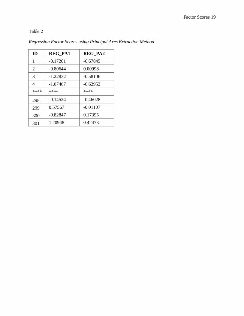
As part of a factor analysis, SPSS calculates factor scores and automatically saves them in

the data file, where they are easily accessible for further analyses (see Table 2). Table 2 is a factor

score matrix for our population of 301 participants on the six variables. All factor scores have a

matrix rank of FNxF. Note that the leftmost column (labeled “ID”) consists of participant

identification. In other words, there is one row for each of our 301 study participants. Thus, each

row in this matrix represents an individual participant‟s factor score for any given number of

factors (in this case, there are two factors). The subscript “N” in the matrix rank represents the fact

that the rows in a factor score matrix represent the study population. The columns (labeled

REG_PA1 and REG_PA2, respectively) represent the two factors that were extracted when a

regression analysis was run with principal axes extraction method (more on extraction methods to

come). You can manually change these variable names in the SPSS data file, if you wish. Note that

the “F” in the matrix rank denotes that the columns in a factor score matrix represent the factors.

This rank could be rewritten as F301x2 to represent the 301 participants and 2 factors.

Factor Scores 6

Factor Scores vs. Factors

Students sometimes confuse factor scores with the factors themselves (Wells, 1999).

Factors scores are the composite (latent) scores for each subject on each factor, which is a grouping

of measured variables. A few distinctions between the two:

1. Factor score matrices (FNxF) and factor matrices (WVxF) have different ranks.

2. Remember that there will be “N" factor scores on each factor (e.g., one factor score for

each person in a given study) and “V” rows in a factor matrix.

3. Factor scores are latent scores on the factors themselves.

4. Factor scores are specific to each research participant on each factor (i.e., each participant

has an individual factor score on each factor).

5. Factors are specific to a group of measured variables.

6. Factor scores will be located in the SPSS data file.

7. Factors will be located in the SPSS output file.

In factor analysis, it is possible to have more than one factor (unlike in multiple regression

where there is only one regression equation). The number of factors “worth keeping” ranges

between 1 to the total number of variables (Thomson, 2004, p. 17). The number of worthy

factors is a subjective call on the noteworthiness of the amount of information or variability the

factor reproduces. Very little variability might not be “worth” taking into account, in many cases.

In addition to the factor score matrix seen in Table 2, SPSS creates a factor matrix that

includes all extracted factors from a factor analysis (see Table 3). The entries in Table 3 are an

indication of how useful each factor is for explaining the variance of the measured variables; but

do not be misled: They ARE NOT FACTOR SCORES! Note that the leftmost, unlabeled column

consists of measured variable names. This signifies that each row in this matrix represents a

Factor Scores 7

measured variable. The subscript “V” in the factor matrix rank represents this fact – the fact that

the rows in a factor matrix represent the variables. The middle and right most columns (labeled “1”

and “2”, respectively) represent the two factors that were extracted from the data set. Note that the

“F” in the matrix rank (i.e., WVxF) denotes that the columns in a factor matrix represent the factors.

This rank could be rewritten F6x2 because there are six measured variables and two factors in this

example.

The factor matrix can sometimes be labeled “component matrix”. In Table 3, the matrix is

labeled “factor matrix” because the extraction method used was principal axes. However, when

principal components extraction method is utilized, the matrix containing the factors is labeled

“component matrix” in the SPSS output. Don‟t be confused by the differing terminology, “factor

matrix” and “component matrix” both illustrate the factors in a given factor analysis.

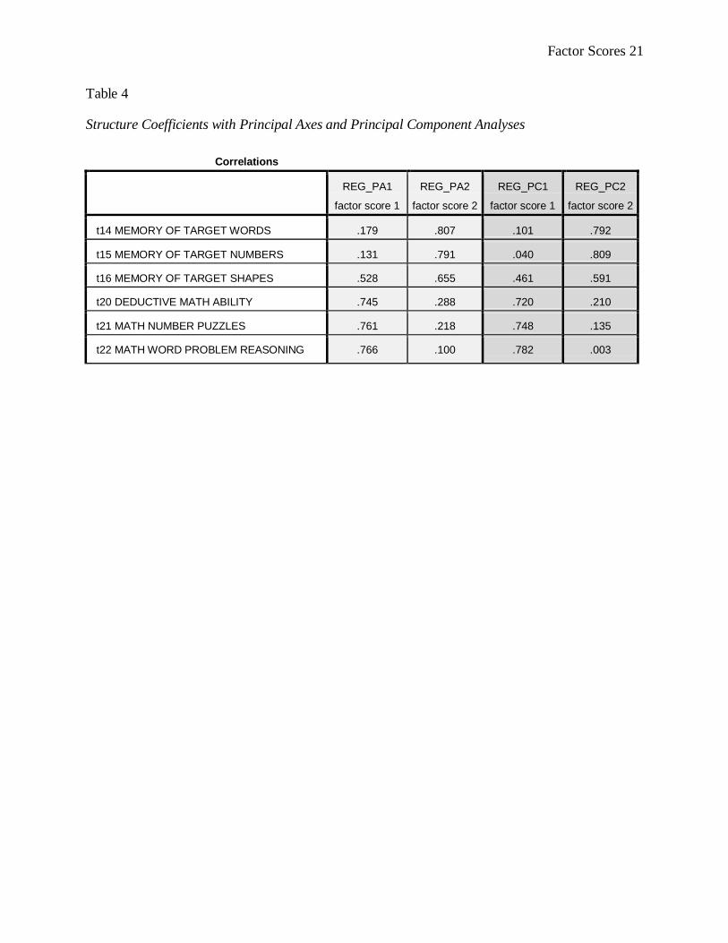
Factor Structure Coefficients

Factor structure coefficients are always, always called structure coefficients in GLM

analyses. They are the bivariate correlations (e.g., Pearson‟s r; or correlation between x and Ŷ)

between measured variables (e.g., x) and their composite variables (e.g., Ŷ). When factors are

perfectly uncorrelated, structure coefficients are exactly equal to pattern coefficients and can be

labeled pattern/structure coefficients. The case of perfectly uncorrelated factors is analogous to

case #1 in regression, when only pattern coefficients (i.e., beta weights) or structure coefficients

(Pearson‟s r) are needed for result interpretation, since they are exactly equal (Thompson, 2004).

See Table 4 for the factor structure coefficients for our current research example. There are two

sets of factor structure coefficients in this example: One set using the principal components

extraction method (more on extraction methods later), in the two far right columns labeled

REG_PC1 and REG_PC2 and a second set utilizing the principal axes extraction method, labeled

Factor Scores 8

REG_PA1 and REG_PA2. Note that both extraction methods identified two factors, but the

individual factor structure coefficients differ between the two methods.

Communality Coefficients (h2)

A communality coefficient measures how much variance in a measured variable the

factors, as a set, reproduce. They answer the question: “How well do the factors represent the

measured variables?” Or, conversely: “How well do the measured variables load into the factors?”

When h2 = 0%, then the variable of interest in not being represented in the factors and additional

factors may need to be extracted. Note that when h2 > 100%, it is labeled a Heywood case, an

indication of a statistically inadmissible result, as reliability of scores is bound by 0% and 100%

(Thompson, 2004). Additionally, communality coefficients provide a “„lower bound‟ estimate of

reliability of the scores on the variable” (Thompson, 2004, p. 20). That is, if h2 = 50%; we may

discern that the reliability of the scores on the variable is at least 50%.

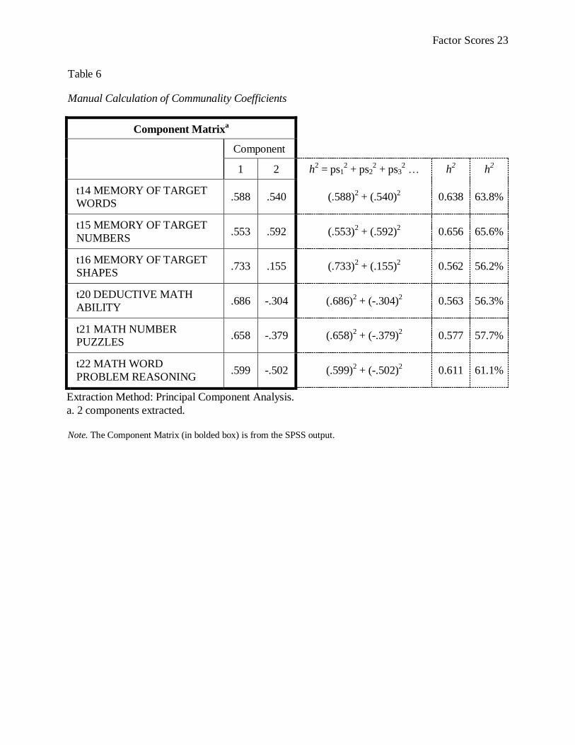
SPSS computes communality coefficients as part of its factor analysis and conveniently

prints them in the output file (see Table 5). The communality coefficients are located in the far

right column of Tabe 5, labeled “extraction”. For example, the communality coefficient for

variable t14 is .638, or 63.8%, because communality coefficients (h2) are already squared. While it

is convenient that SPSS computes these communality coefficients for us, we have the ability to

compute them for ourselves by summing the pattern/structure coefficients:

h2 = ps1

2 + ps2

2 + ps3

2 + psn

2…

This equation is only for uncorrelated factors, which is the aim of factor analyses. Because the

factors in our example are uncorrelated, we can use this formula to calculate the communality

coefficients for ourselves (see Table 6). To calculate communality coefficient values, we need the

component (or factor) matrix from the SPSS output (the bolded portion of Table 6). Then, we

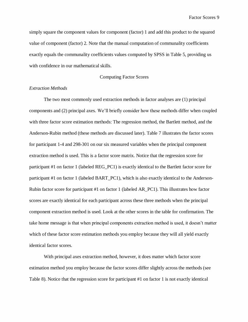
Factor Scores 9

simply square the component values for component (factor) 1 and add this product to the squared

value of component (factor) 2. Note that the manual computation of communality coefficients

exactly equals the communality coefficients values computed by SPSS in Table 5, providing us

with confidence in our mathematical skills.

Computing Factor Scores

Extraction Methods

The two most commonly used extraction methods in factor analyses are (1) principal

components and (2) principal axes. We‟ll briefly consider how these methods differ when coupled

with three factor score estimation methods: The regression method, the Bartlett method, and the

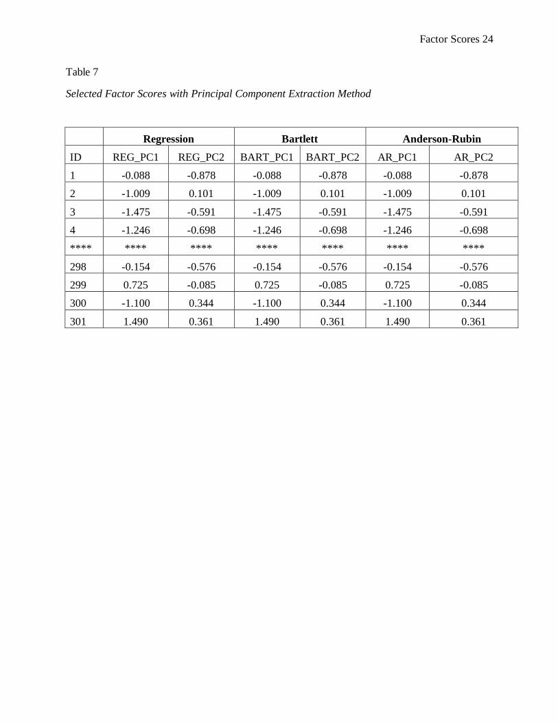
Anderson-Rubin method (these methods are discussed later). Table 7 illustrates the factor scores

for participant 1-4 and 298-301 on our six measured variables when the principal component

extraction method is used. This is a factor score matrix. Notice that the regression score for

participant #1 on factor 1 (labeled REG_PC1) is exactly identical to the Bartlett factor score for

participant #1 on factor 1 (labeled BART_PC1), which is also exactly identical to the Anderson-

Rubin factor score for participant #1 on factor 1 (labeled AR_PC1). This illustrates how factor

scores are exactly identical for each participant across these three methods when the principal

component extraction method is used. Look at the other scores in the table for confirmation. The

take home message is that when principal components extraction method is used, it doesn‟t matter

which of these factor score estimation methods you employ because they will all yield exactly

identical factor scores.

With principal axes extraction method, however, it does matter which factor score

estimation method you employ because the factor scores differ slightly across the methods (see

Table 8). Notice that the regression score for participant #1 on factor 1 is not exactly identical

Factor Scores 10

across all three methods (-0.172 with regression; -0.021 with Bartlett; -0.118 with Anderson-

Rubin). Indeed, the factor scores vary for all participants across the methods. Thus, when principal

axes extraction method is used, it does matter which factor score estimation method is used.

A further illustration of the difference between principal components and principal axes is

evident when a correlation between the two extracted factors is calculated. Remember that SPSS

saves factor scores in the data file, so further analyses may easily be run. To run a correlation

between extracted factors – in our current example there are 2 – the following SPSS syntax can be

utilized:

CORRELATIONS

/VARIABLES=REG_PA1 REG_PA2

/PRINT=TWOTAIL NOSIG

/STATISTICS DESCRIPTIVES

/MISSING=PAIRWISE.

CORRELATIONS

/VARIABLES=REG_PC1 REG_PC2

/PRINT=TWOTAIL NOSIG

/STATISTICS DESCRIPTIVES

/MISSING=PAIRWISE.

Note that the first correlation analysis is between the two factors, using principal axes

(REG_PA1 and REG_PA2), while the second analysis uses principal components (REG_PC1 and

REG_PC2). Regression is the factor score extraction method for each, but Bartlett or Anderson-

Rubin could also have been utilized. With the principal component method, the two extracted

factors are perfectly uncorrelated with one another (see Table 9), which is desirable as we prefer

factors that are perfectly uncorrelated with one another.

Another appealing characteristic of principal components for factor score computation is

that the factor score correlations exactly match the factors themselves. For example, the rotated

component matrix created by SPSS with principal components (in Tables 1, 3, and 4) is identical to

the Pearson‟s r correlation between the measured variables and factor scores with all three factor

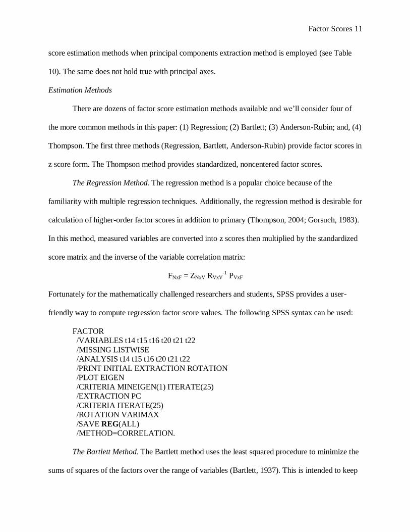
Factor Scores 11

score estimation methods when principal components extraction method is employed (see Table

10). The same does not hold true with principal axes.

Estimation Methods

There are dozens of factor score estimation methods available and we‟ll consider four of

the more common methods in this paper: (1) Regression; (2) Bartlett; (3) Anderson-Rubin; and, (4)

Thompson. The first three methods (Regression, Bartlett, Anderson-Rubin) provide factor scores in

z score form. The Thompson method provides standardized, noncentered factor scores.

The Regression Method. The regression method is a popular choice because of the

familiarity with multiple regression techniques. Additionally, the regression method is desirable for

calculation of higher-order factor scores in addition to primary (Thompson, 2004; Gorsuch, 1983).

In this method, measured variables are converted into z scores then multiplied by the standardized

score matrix and the inverse of the variable correlation matrix:

FNxF = ZNxV RVxV-1

PVxF

Fortunately for the mathematically challenged researchers and students, SPSS provides a user-

friendly way to compute regression factor score values. The following SPSS syntax can be used:

FACTOR

/VARIABLES t14 t15 t16 t20 t21 t22

/MISSING LISTWISE

/ANALYSIS t14 t15 t16 t20 t21 t22

/PRINT INITIAL EXTRACTION ROTATION

/PLOT EIGEN

/CRITERIA MINEIGEN(1) ITERATE(25)

/EXTRACTION PC

/CRITERIA ITERATE(25)

/ROTATION VARIMAX

/SAVE REG(ALL)

/METHOD=CORRELATION.

The Bartlett Method. The Bartlett method uses the least squared procedure to minimize the

sums of squares of the factors over the range of variables (Bartlett, 1937). This is intended to keep

Factor Scores 12

noncommon factors “in their place” so that they are only used to explain differences between

observed scores and reproduced scores (Gorsuch, 1983, p. 264). The Bartlett method leads to high

correlation between factor scores and factors being estimated.

The Bartlett method is both univocal and unbiased. Univocal means that each measured

variable only speaks through one factor. It is desirable for a variable to only be highly correlated

with one factor so that we have a simple structure. When variables speak through multiple factors,

the factors might be too correlated with one another to be the best selection of factors. When

variables speak through multiple factors, we need to look at our factors to determine if they are, in

fact, the best factors for our given sample. Our aim is uncorrelated factors. Unbiased refers to the

capacity of repeated samples invoking a statistic to yield accurate estimates of corresponding

parameters. For example, if we draw infinitely many random samples from a population, all at the

same time, the averages of the sample means will equal the population mean (Thompson, 2006).

To run the Bartlett method in SPSS, the following syntax can be used:

FACTOR


/MISSING LISTWISE



/PLOT EIGEN


/EXTRACTION PC


/ROTATION VARIMAX

/SAVE BART(ALL)


The Anderson-Rubin Method. The Anderson-Rubin method is similar to the Bartlett

method, but more complex. The factor scores must be orthogonal to utilize the Anderson-Rubin

method, which generates factor estimates whose correlations form an Identity Matrix (Wells,

Factor Scores 13

1999). This method is neither univocal nor unbiased. (Anderson & Rubin, 1956; Thompson, 2004;

Wells, 1999). To run the Anderson-Rubin method in SPSS, the following syntax can be utilized:

FACTOR


/MISSING LISTWISE



/PLOT EIGEN


/EXTRACTION PC


/ROTATION VARIMAX

/SAVE AR(ALL)


The Thompson Method. Conventional methods (e.g., Regression, Bartlett, Anderson-

Rubin) produce factor score estimates in a z score form, with means equal to zero and a standard

deviation score equal to one (i.e., standardized). Z score form is not useful for comparison of factor

scores across factors within the whole data set:

While in many applications this score form is appealing, the result does preclude

comparison of the mean factor score on any given factor with the means on other factor

scores, because the means of each set of factor scores will have been set to zero…This is

unfortunate, because sometimes we wish to compare means on factor scores across factors

to make some judgment regarding the relative importance of given factors (Thompson,

1993, p. 1129).

The Thompson methods solves this issue of comparison of means across factor scores by

calculating factor scores that are still standardized but with means that are determined by the

original variable means. The benefit of the Thompson method, as described by its creator is its

ability produce standardized, noncentered factor scores that permit comparison across factors.

Execution of the Thompson method in SPSS has three steps: (1) Z scores must be computed; (2)

Factor Scores 14

the original measured variable means must be added back onto the z scores; and, (3) the weight

matrix (i.e., factor/component score coefficient matrix) must be applied to the standardized,

noncentered scores:

(1) DESCRIPTIVES variables=t14 t15 t16 t20 t21 t22/SAVE.

(2) compute ct14 = zt14 + 175.15 .

compute ct15 = zt15 + 90.01 .

compute ct16 = zt16 + 102.52 .

compute ct20 = zt20 + 26.89 .

compute ct21 = zt21 + 14.25 .

compute ct22 = zt22 + 26.24 .

print formats zt14 to ct22 (F7.2) .

list variables=id zt14 to ct22/cases=10 .

DESCRIPTIVES variables= zt14 to ct22 .

(3) compute BTscr1 = (-.119 * ct14) + (-.159 * ct15) + (.142 * ct16) + (.383 * ct20) +

(.417 * ct21) + (.467 * ct22) .

compute BTscr2 = (.512 * ct14) + (.537 * ct15) + (.295 * ct16) + (-.021 * ct20) + (-

.078 * ct21) + (-.175 * ct22) .

print formats BTscr1 BTscr2 (F8.3) .

A comparison of regression factor scores and Thompson factor scores is available in Table

11. Note that participant #1‟s Thompson factor scores on factor 1 (labeled BTscr1) and factor 2

(labeled BTscr2) are 235.503 and 94.497, respectively. Because the Thompson factor scores allow

for mean comparisons across factors, we compare this individual‟s factor scores with the mean

score on each individual factor. This provides a comparison of how one participant‟s scores on a

factor compare to other participants.

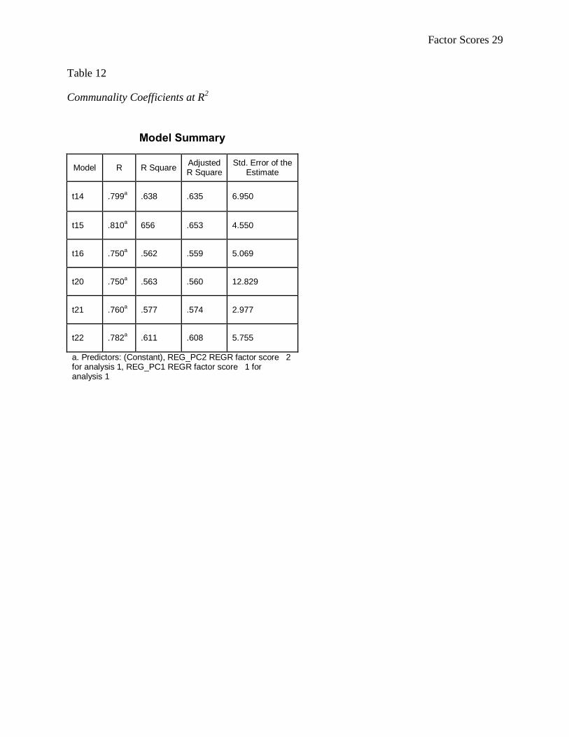
Communality Coefficients as R2

We know that another GLM principal is that all analyses compute r2–type effect sizes

(Thompson, 2006). In factor analyses, the communality coefficients (h2) can be the R

2–type effect

size (Thompson, 2004). We noted that communality coefficients signify how much of measured

variables‟ variance the factors as a set can reproduce. Stated otherwise, they indicate how much of

the measured variables‟ variance was useful in delineating the extracted factors. With orthogonal

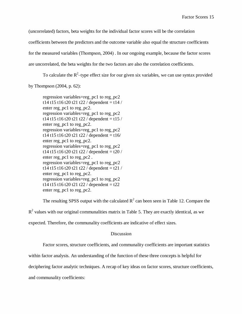
Factor Scores 15

(uncorrelated) factors, beta weights for the individual factor scores will be the correlation

coefficients between the predictors and the outcome variable also equal the structure coefficients

for the measured variables (Thompson, 2004) . In our ongoing example, because the factor scores

are uncorrelated, the beta weights for the two factors are also the correlation coefficients.

To calculate the R2–type effect size for our given six variables, we can use syntax provided

by Thompson (2004, p. 62):

regression variables=reg_pc1 to reg_pc2

t14 t15 t16 t20 t21 t22 / dependent = t14 /

enter reg_pc1 to reg_pc2.





t14 t15 t16 t20 t21 t22 / dependent = t16/




enter reg_pc1 to reg_pc2 .





t14 t15 t16 t20 t21 t22 / dependent = t22


The resulting SPSS output with the calculated R2 can been seen in Table 12. Compare the

R2 values with our original communalities matrix in Table 5. They are exactly identical, as we

expected. Therefore, the communality coefficients are indicative of effect sizes.

Discussion

Factor scores, structure coefficients, and communality coefficients are important statistics

within factor analysis. An understanding of the function of these three concepts is helpful for

deciphering factor analytic techniques. A recap of key ideas on factor scores, structure coefficients,

and communality coefficients:

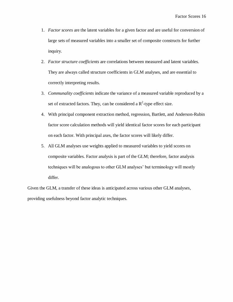
Factor Scores 16

1. Factor scores are the latent variables for a given factor and are useful for conversion of

large sets of measured variables into a smaller set of composite constructs for further

inquiry.

2. Factor structure coefficients are correlations between measured and latent variables.

They are always called structure coefficients in GLM analyses, and are essential to

correctly interpreting results.

3. Communality coefficients indicate the variance of a measured variable reproduced by a

set of extracted factors. They, can be considered a R2-type effect size.

4. With principal component extraction method, regression, Bartlett, and Anderson-Rubin

factor score calculation methods will yield identical factor scores for each participant

on each factor. With principal axes, the factor scores will likely differ.

5. All GLM analyses use weights applied to measured variables to yield scores on

composite variables. Factor analysis is part of the GLM; therefore, factor analysis

techniques will be analogous to other GLM analyses‟ but terminology will mostly

differ.

Given the GLM, a transfer of these ideas is anticipated across various other GLM analyses,

providing usefulness beyond factor analytic techniques.

Factor Scores 17

References

Anderson, R. D., & Rubin, H. (1956). Statistical inference in factor analysis. Proceedings of the

Third Berkeley Symposium of Mathematical Statistics and Probability, 5, 111-150.

Bartlett, M. S. (1937). The statistical conception of mental factors. British Journal of

Psychology, 28 (1), 97-104.

Gorsuch, R. L. (1983). Factor analysis (2nd

ed.). Hillsdale, NJ: Erlbaum.

Thompson, B. (1993). Calculation of standardized, noncentered factor scores: An alternative to

conventional factor scores. Perceptual and Motor Skills, 77 (3), 1128-1130.

Thompson, B. (2004). Exploratory and confirmatory factor analysis: Understanding concepts and

applications. Washington, D.C.: American Psychological Association.

Thompson, B. (2006). Foundations of behavioral statistics: An insight-based approach. New York:

Guilford.

Wells, R.D. (1999). Factor scores and factor structure. In Advances in social science methodology,

(Vol. 5, pp. 123-138). Greenwich, CT: JAI Press

Factor Scores 18

Table 1

Pattern Coefficient Matrices with Principal Axes and Principal Component Analyses

Rotated Component Matrixa

Component

1 2

t14 MEMORY OF TARGET WORDS

.101 .792

t15 MEMORY OF TARGET NUMBERS

.040 .809

t16 MEMORY OF TARGET SHAPES

.461 .591

t20 DEDUCTIVE MATH ABILITY

.720 .210

t21 MATH NUMBER PUZZLES

.748 .135

t22 MATH WORD PROBLEM REASONING

.782 .003

Extraction Method: Principal Component Analysis. Rotation Method: Varimax with Kaiser Normalization.

a. Rotation converged in 3 iterations.

Rotated Factor Matrixa

Factor

1 2

t14 MEMORY OF TARGET WORDS

.143 .623

t15 MEMORY OF TARGET NUMBERS

.104 .611

t16 MEMORY OF TARGET SHAPES

.421 .506

t20 DEDUCTIVE MATH ABILITY

.594 .222

t21 MATH NUMBER PUZZLES

.607 .168

t22 MATH WORD PROBLEM REASONING

.610 .077

Extraction Method: Principal Axis Factoring. Rotation Method: Varimax with Kaiser Normalization.


Factor Scores 19

Table 2

Regression Factor Scores using Principal Axes Extraction Method

ID REG_PA1 REG_PA2

1 -0.17201 -0.67845

2 -0.80644 0.00998

3 -1.22832 -0.58106

4 -1.07467 -0.62952

**** **** ****

298 -0.14524 -0.46028

299 0.57567 -0.01107

300 -0.82847 0.17395

301 1.20948 0.42473

Factor Scores 20

Table 3

Factor Matrices from SPSS with Principal Axes and Principal Component Analyses

Rotated Factor Matrixa

Factor

1 2

t14 MEMORY OF TARGET

WORDS

.143 .623


NUMBERS

.104 .611


SHAPES

.421 .506

t20 DEDUCTIVE MATH

ABILITY

.594 .222

t21 MATH NUMBER

PUZZLES

.607 .168

t22 MATH WORD PROBLEM

REASONING

.610 .077

Extraction Method: Principal Axis Factoring.

Rotation Method: Varimax with Kaiser Normalization.


Rotated Component Matrixa

Component

1 2


WORDS

.101 .792


NUMBERS

.040 .809


SHAPES

.461 .591

t20 DEDUCTIVE MATH

ABILITY

.720 .210

t21 MATH NUMBER

PUZZLES

.748 .135


REASONING

.782 .003

Extraction Method: Principal Component Analysis.

Rotation Method: Varimax with Kaiser Normalization.


Factor Scores 21

Table 4

Structure Coefficients with Principal Axes and Principal Component Analyses

Correlations

REG_PA1

factor score 1

REG_PA2

factor score 2

REG_PC1

factor score 1

REG_PC2

factor score 2

t14 MEMORY OF TARGET WORDS .179 .807 .101 .792

t15 MEMORY OF TARGET NUMBERS .131 .791 .040 .809

t16 MEMORY OF TARGET SHAPES .528 .655 .461 .591

t20 DEDUCTIVE MATH ABILITY .745 .288 .720 .210

t21 MATH NUMBER PUZZLES .761 .218 .748 .135

t22 MATH WORD PROBLEM REASONING .766 .100 .782 .003

Factor Scores 22

Table 5

Communality Coefficients with Principal Component Analysis

Communalities

Initial Extraction


WORDS

1.000 .638


NUMBERS

1.000 .656


SHAPES

1.000 .562

t20 DEDUCTIVE MATH

ABILITY

1.000 .563

t21 MATH NUMBER

PUZZLES

1.000 .577


REASONING

1.000 .611


Factor Scores 23

Table 6

Manual Calculation of Communality Coefficients

Component Matrixa

Component

1 2 h2 = ps1

2 + ps2

2 + ps3

2 … h

2 h

2


WORDS .588 .540 (.588)

2 + (.540)

2 0.638 63.8%


NUMBERS .553 .592 (.553)

2 + (.592)

2 0.656 65.6%


SHAPES .733 .155 (.733)

2 + (.155)

2 0.562 56.2%

t20 DEDUCTIVE MATH

ABILITY .686 -.304 (.686)

2 + (-.304)

2 0.563 56.3%

t21 MATH NUMBER

PUZZLES .658 -.379 (.658)

2 + (-.379)

2 0.577 57.7%

t22 MATH WORD

PROBLEM REASONING .599 -.502 (.599)

2 + (-.502)

2 0.611 61.1%


a. 2 components extracted.

Note. The Component Matrix (in bolded box) is from the SPSS output.

Factor Scores 24

Table 7

Selected Factor Scores with Principal Component Extraction Method

Regression Bartlett Anderson-Rubin

ID REG_PC1 REG_PC2 BART_PC1 BART_PC2 AR_PC1 AR_PC2

1 -0.088 -0.878 -0.088 -0.878 -0.088 -0.878

2 -1.009 0.101 -1.009 0.101 -1.009 0.101

3 -1.475 -0.591 -1.475 -0.591 -1.475 -0.591

4 -1.246 -0.698 -1.246 -0.698 -1.246 -0.698

**** **** **** **** **** **** ****

298 -0.154 -0.576 -0.154 -0.576 -0.154 -0.576

299 0.725 -0.085 0.725 -0.085 0.725 -0.085

300 -1.100 0.344 -1.100 0.344 -1.100 0.344

301 1.490 0.361 1.490 0.361 1.490 0.361

Factor Scores 25

Table 8

Selected Factor Scores with Principal Axes Extraction Method

Regression Bartlett Anderson-Rubin

ID REG_PA1 REG_PA2 BART_PA1 BART_PA2 AR_PA1 AR_PA2

1 -0.172 -0.678 -0.021 -1.132 -0.118 -0.869

2 -0.806 0.010 -1.343 0.335 -1.034 0.136

3 -1.228 -0.581 -1.812 -0.549 -1.485 -0.583

4 -1.075 -0.630 -1.540 -0.693 -1.282 -0.669

**** **** **** **** **** **** ****

298 -0.145 -0.460 -0.060 -0.761 -0.116 -0.588

299 0.576 -0.011 0.961 -0.245 0.739 -0.101

300 -0.828 0.174 -1.442 0.631 -1.086 0.354

301 1.209 0.425 1.839 0.280 1.482 0.380

Factor Scores 26

Correlations

REG_PC1

REGR factor

score 1 for

analysis 1

REG_PC2

REGR factor

score 2 for

analysis 1

REG_PC1 REGR factor

score 1 for analysis 1

Pearson Correlation 1 .000

Sig. (2-tailed) 1.000

N 301 301

REG_PC2 REGR factor


Pearson Correlation .000 1

Sig. (2-tailed) 1.000

N 301 301

Table 9

Correlations between Factors in Principal Component and Principal Axes

Correlations

REG_PA1 REGR

factor score 1

for analysis 1

REG_PA2 REGR

factor score 2

for analysis 1

REG_PA1 REGR factor


Pearson Correlation 1 .228**

Sig. (2-tailed) .000

N 301 301

REG_PA2 REGR factor


Pearson Correlation .228** 1

Sig. (2-tailed) .000

N 301 301

**. Correlation is significant at the 0.01 level (2-tailed).

Factor Scores 27

Table 10

Pearson’s r Correlation Matrix

Pearson‟s r values between Measured Variables and Factor Scores with Principal

Component Extraction Method

REG_PC1 REG_PC2 BART_PC1 BART_PC2 AR_PC1 AR_PC2

t14 0.101 0.792 0.101 0.792 0.101 0.792

t15 0.040 0.809 0.040 0.809 0.040 0.809

t16 0.461 0.591 0.461 0.591 0.461 0.591

t20 0.720 0.210 0.720 0.210 0.720 0.210

t21 0.748 0.135 0.748 0.135 0.748 0.135

t22 0.782 0.003 0.782 0.003 0.782 0.003

Factor Scores 28

Table 11

Comparison of Regression and Thompson Factor Scores

Regression Thompson

ID REG_PA1 REG_PA2 BTscr1 BTscr2

1 -0.17201 -0.67845 235.503 94.497

2 -0.80644 0.00998 235.369 95.569

3 -1.22832 -0.58106 233.653 95.379

4 -1.07467 -0.62952 233.874 95.212

**** **** **** **** ****

298 -0.14524 -0.46028 235.834 94.685

299 0.57567 -0.01107 237.929 94.533

300 -0.82847 0.17395 235.565 95.743

301 1.20948 0.42473 239.793 94.427

Factor Scores 29

Table 12

Communality Coefficients at R2

Model Summary

Model R R Square Adjusted R Square

Std. Error of the Estimate

t14 .799a .638 .635 6.950

t15 .810a 656 .653 4.550

t16 .750a .562 .559 5.069

t20 .750a .563 .560 12.829

t21 .760a .577 .574 2.977

t22 .782a .611 .608 5.755

a. Predictors: (Constant), REG_PC2 REGR factor score 2 for analysis 1, REG_PC1 REGR factor score 1 for analysis 1

Factor Scores 30

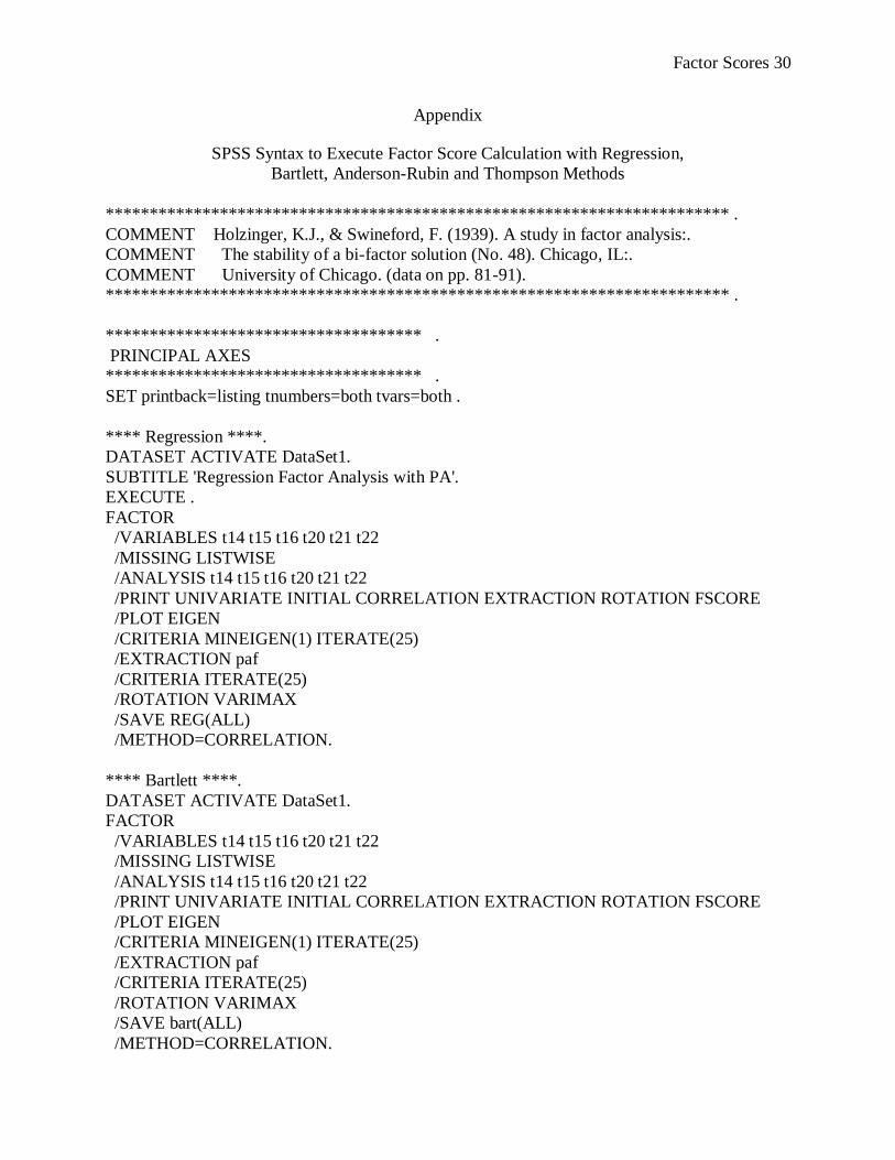
Appendix

SPSS Syntax to Execute Factor Score Calculation with Regression,

Bartlett, Anderson-Rubin and Thompson Methods

*********************************************************************** .

COMMENT Holzinger, K.J., & Swineford, F. (1939). A study in factor analysis:.

COMMENT The stability of a bi-factor solution (No. 48). Chicago, IL:.

COMMENT University of Chicago. (data on pp. 81-91).

*********************************************************************** .

************************************ .

PRINCIPAL AXES

************************************ .

SET printback=listing tnumbers=both tvars=both .

**** Regression ****.

DATASET ACTIVATE DataSet1.

SUBTITLE 'Regression Factor Analysis with PA'.

EXECUTE .

FACTOR


/MISSING LISTWISE


/PRINT UNIVARIATE INITIAL CORRELATION EXTRACTION ROTATION FSCORE

/PLOT EIGEN


/EXTRACTION paf


/ROTATION VARIMAX

/SAVE REG(ALL)


**** Bartlett ****.


FACTOR


/MISSING LISTWISE



/PLOT EIGEN


/EXTRACTION paf


/ROTATION VARIMAX

/SAVE bart(ALL)


Factor Scores 31

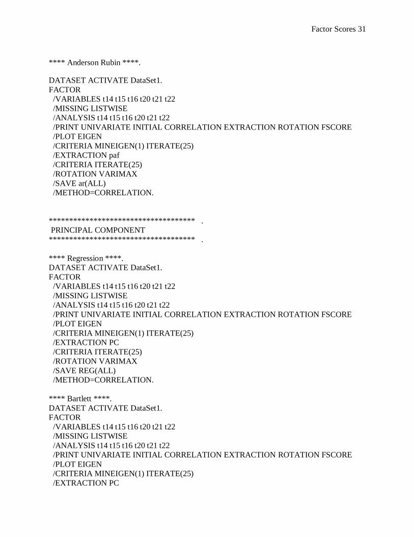
**** Anderson Rubin ****.


FACTOR


/MISSING LISTWISE



/PLOT EIGEN


/EXTRACTION paf


/ROTATION VARIMAX

/SAVE ar(ALL)


************************************ .

PRINCIPAL COMPONENT

************************************ .

**** Regression ****.


FACTOR


/MISSING LISTWISE



/PLOT EIGEN


/EXTRACTION PC


/ROTATION VARIMAX

/SAVE REG(ALL)


**** Bartlett ****.


FACTOR


/MISSING LISTWISE



/PLOT EIGEN


/EXTRACTION PC

Factor Scores 32


/ROTATION VARIMAX

/SAVE bart(ALL)


**** Anderson Rubin ****.


FACTOR


/MISSING LISTWISE



/PLOT EIGEN


/EXTRACTION PC


/ROTATION VARIMAX

/SAVE ar(ALL)


************************************************ .

THOMPSON METHOD

************************************************ .

**** (1) compute z scores **** .

DESCRIPTIVES variables=t14 t15 t16 t20 t21 t22/save .

**** (2) add original measured variable means back onto z scores **** .

compute ct14 = zt14 + 175.15 .

compute ct15 = zt15 + 90.01 .

compute ct16 = zt16 + 102.52 .

compute ct20 = zt20 + 26.89 .

compute ct21 = zt21 + 14.25 .

compute ct22 = zt22 + 26.24 .

print formats zt14 to ct22 (F7.2) .

list variables=id zt14 to ct22/cases=10 .

DESCRIPTIVES variables= zt14 to ct22 .

**** (3) apply weight matrix **** .

compute BTscr1 = (-.119 * ct14) + (-.159 * ct15) + (.142 * ct16) + (.383 * ct20) + (.417 * ct21)

+ (.467 * ct22) .

compute BTscr2 = (.512 * ct14) + (.537 * ct15) + (.295 * ct16) + (-.021 * ct20) + (-.078 * ct21)

+ (-.175 * ct22) .

print formats BTscr1 BTscr2 (F8.3) .

factor scores, structure and communality coefficients: a ... scores, structure and communality...

Documents