factor structure in commodity futures return and

Department of Economics and Business

Aarhus University

Fuglesangs Allé 4

DK-8210 Aarhus V

Denmark

Email: [email protected]

Tel: +45 8716 5515

Factor Structure in Commodity Futures Return and Volatility

Peter Christoffersen, Asger Lunde and Kasper V. Olesen

CREATES Research Paper 2014-31

mailto:[email protected]

Factor Structure in Commodity FuturesReturn and Volatility*

Peter Christoffersena Asger Lundeb

Kasper V. Olesenb

aRotman School of Management, University of Toronto, CBS & CREATES

bAarhus University, Department of Economics and Business & CREATES

September 8, 2014

Abstract

Using data on more than 750 million futures trades during 2004-2013, we analyze eight

stylized facts of commodity price and volatility dynamics in the post financialization period.

We pay particular attention to the factor structure in returns and volatility and to commodity

market integration with the equity market. We find evidence of a factor structure in daily

commodity futures returns. However, the factor structure in daily commodity futures

volatility is even stronger than in returns. When computing model-free realized commodity

betas with the stock market we find that they were high during 2008-2010 but have since

returned to the pre-crisis level close to zero. The common factor in commodity volatility is

nevertheless clearly related to stock market volatility. We conclude that, while commodity

markets appear to again be segmented from the equity market when only returns are

considered, commodity volatility indicates a nontrivial degree of market integration.

Keywords: Factor structure, financial volatility, beta, high-frequency data, commodities,

financialization

JEL Classifications: G13, Q02

*All authors acknowledge support from CREATES - Center for Research in Econometric Analysisof Time Series (DNRF78), funded by the Danish National Research Foundation. Christoffersen wasalso supported by Bank of Canada, GRI, and the Social Sciences, and Humanities Research Council ofCanada. Lunde and Olesen thank the AU Ideas Pilot Center, Stochastic and Econometric Analysis ofCommodity Markets, for financial support. Address correspondence to Peter Christoffersen, RotmanSchool of Management, University of Toronto, 105 St. George St., M5S 3E6 Toronto, Canada; E-mailaddress: [email protected].

1 Introduction

The deregulation of commodity markets in the early 2000s, and the subsequent large

inflows of investment capital to commodity futures and related securities, has sparked a

heated debate in the popular press as well as in academia. A large part of the discussion

of this so-called “financialization” of commodity markets has focused on bubbles in

commodity prices and increases in commodity price volatility supposedly caused by

futures market trading. The relationship between commodity futures and other asset

markets, and in particular risk sharing across markets, has received substantial attention

in academia. Cheng & Xiong (2013) provide an excellent overview of existing work on

the financialization of commodity futures markets.

We use more than 750 million commodity futures transactions to construct daily re-

alized volatility for fifteen commodities during the 2004-2013 period. To our knowledge,

we are the first to construct realized covariances for each commodity with the stock

market which we use to develop time-varying but model-free stock market betas as

well as systematic risk contributions for each commodity. We use these measures along

with daily futures returns to address the following research questions:

First, what are the stylized facts of commodity futures returns and volatility post

financialization? Second, is there a factor structure in commodity futures returns? Third,

is the stock market driving the common component of commodity futures returns?

Fourth, do the stock market betas of commodity futures returns vary significantly over

time? Fifth, does the ratio of commodity futures return volatility explained by the

stock market beta change over time? Sixth, is there a factor structure in commodity

futures volatility? Finally, is stock market volatility driving the common component of

commodity futures volatility? The stylized facts that we uncover are:

Fact #1: Daily realized commodity futures volatility has extremely high persistence.

Fact #2: The logarithm of realized commodity futures volatility is close to normally distributed.

Fact #3: There is some evidence of a factor structure in daily commodity futures returns

excluding meats.

2

Fact #4: The factor structure in daily commodity futures volatility is much stronger than the

factor structure in returns.

Fact #5: There is little evidence of a time-trend in the degree of integration across commodity

futures markets during the 2004-2013 period.

Fact #6: The strong common factor in commodity volatility is largely driven by stock market

volatility.

Fact #7: Commodity betas with the stock market were high during 2008-2010 but have since

returned to a level close to zero.

Fact #8: Commodity futures returns standardized by expected realized volatility are closer to

normally distributed than the returns themselves but still display leptokurtosis.

Most authors, including Baker (2014), Baker & Routledge (2012), and Hamilton & Wu

(2014), date the financialization to take effect sometime in the 2004-2005 period. We

follow these papers and begin our analysis in January 2004. Our analysis is based on

approximately 3/4 billion trades in commodity futures contracts observed from January

2004 through December 2013. We choose the three most heavily traded commodities in

the energy, metals, grains, softs, and meats categories for a total of 15 futures contracts.

Our work builds heavily on recent advances in model-free volatility and covariance

measurement using high-frequency data. See for example Andersen, Bollerslev, Christof-

fersen & Diebold (2013), Barndorff-Nielsen & Shephard (2007), and Hansen & Lunde

(2011) for recent surveys.

Bakshi, Gao & Rossi (2013) develop a three-factor commodity pricing model, using

the average commodity return, a basis spread factor, and a momentum factor. They find

that the model captures both the cross-sectional and time-series variation in commodity

returns. Szymanowska, De Roon, Nijman & Van Den Goorbergh (2014) also find that

the basis spread factor explains the cross-section of commodity returns. Daskalaki,

Kostakis & Skiadopoulos (2014) also explore common factors in the cross-section of

commodity futures returns. They test various asset pricing models motivated either

by the traditional empirical equity market studies, or by available commodity pricing

theories. They find that none of the models they investigate are successful and conclude

3

that commodity markets are heterogeneous and segmented from the equity market.

From the apparent conflict in these recent studies we conclude that the factor structure

of commodity returns needs to be studied further.

The evidence on the integration of commodity and equity markets is also mixed.

For early evidence on segmentation, see Bessembinder (1992), Bessembinder & Chan

(1992), and Gorton & Rouwenhorst (2006). For recent evidence on integration, see Tang

& Xiong (2012), Henderson, Pearson & Wang (2013), Basak & Pavlova (2014), and

Singleton (2014). We contribute to this discussion by constructing daily model-free

realized market betas from high-frequency returns on commodity futures and market

index futures.

Inspired by Longin & Solnik (2001) and Ang & Chen (2002) who study equity

markets, we analyze the threshold correlations between commodity futures returns

and stock market returns. We find strong evidence of tail-dependence between com-

modity and equity market returns suggesting important nonlinear and non-normal

dependencies between commodity and equity markets.

In recent work focusing on the U.S. equity market, Chen & Petkova (2012), Duarte,

Kamara, Siegel & Sun (2014), and Herskovic, Kelly, Lustig & Van Nieuwerburgh (2014)

find strong evidence of factor structure in idiosyncratic volatility. Herskovic et al. (2014)

use daily data to compute annual firm-specific realized volatilities on a large number of

stocks. They then look for and find strong commonality in the volatility of individual

equities. The commonality in equity volatility is strong even after the market factor is

removed. This work is important because it has the potential to explain the so-called risk

anomaly documented in Ang, Hodrick, Xing & Zhang (2006) and Ang, Hodrick, Xing

& Zhang (2009) showing that stocks with low volatility this quarter have high returns

next month and vice versa. Inspired by this equity market literature, we investigate

the factor structure of individual commodity volatility. We find strong evidence of a

common factor in daily commodity futures volatility which we compute from intraday

returns.

Our study complements Tang & Xiong (2012) who focus on the connection between

the large inflow of commodity index investments and the large increase in commodity

price co-movements. They find that prices of non-energy commodity futures in the

4

United States have become increasingly correlated with oil prices after 2004. Also, they

find that the correlation between commodity returns and the MSCI Emerging Markets

Index has been rising in recent years. Substantial increases in return correlation between

commodities and stocks were also found in Büyüksahin, Haigh & Robe (2010) using the

Dynamic Conditional Correlation (DCC) model of Engle (2002). In recent work, Boons,

Roon & Szymanowska (2013) find that stocks that have high betas with a commodity

index earned a relatively low average return in the pre-financialization period and a

relatively high return in the post-financialization period. We investigate the dynamic

relationship between commodities and the stock market using model-free realized betas.

Our time-varying betas can be viewed as dynamic measures of integration with the

stock market. Our work is therefore related to the research on time-varying integration

of emerging markets, see, for example, Carrieri, Errunza & Hogan (2007) and Bekaert,

Harvey, Lundblad & Siegel (2011).

The remainder of the paper is structured as follows. In Section 2 we describe the

data and the methodology for computing returns and realized volatilities. Section 3

investigates the multivariate properties of commodity futures returns and volatility.

Section 4 analyzes the relationship between commodities and the stock market, and

Section 5 investigates the distributional properties of commodity returns and shocks.

Section 6 concludes. Supplementary figures and tables are placed in the appendix.

2 Constructing Returns and Realized Volatility

We collect data from two main sources. High-frequency data on commodity futures

are obtained from Tick Data Inc. and transaction data on the Spyder ETF are obtained

from the NYSE Trade and Quote (TAQ) database.1 Spyder is used as a proxy for the

stock market index. The commodity futures dataset includes intraday transactions and

quotes for all traded maturities on more than 60 commodities traded across the world.

1Standard & Poor’s Depository Receipt (Spyder) is a tradable security that represents ownership inthe S&P 500 index. By using Spyder, stale price effects associated with using the S&P 500 cash index athigh frequencies are avoided.

5

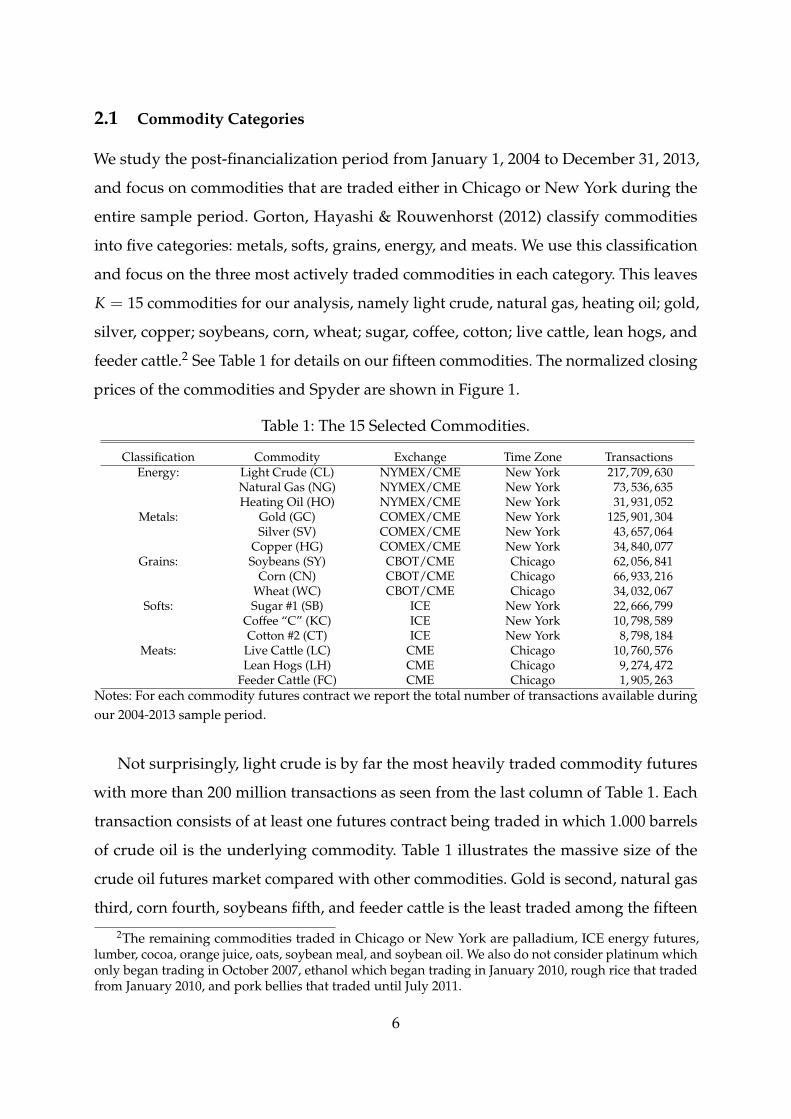
2.1 Commodity Categories

We study the post-financialization period from January 1, 2004 to December 31, 2013,

and focus on commodities that are traded either in Chicago or New York during the

entire sample period. Gorton, Hayashi & Rouwenhorst (2012) classify commodities

into five categories: metals, softs, grains, energy, and meats. We use this classification

and focus on the three most actively traded commodities in each category. This leaves

K = 15 commodities for our analysis, namely light crude, natural gas, heating oil; gold,

silver, copper; soybeans, corn, wheat; sugar, coffee, cotton; live cattle, lean hogs, and

feeder cattle.2 See Table 1 for details on our fifteen commodities. The normalized closing

prices of the commodities and Spyder are shown in Figure 1.

Table 1: The 15 Selected Commodities.

Classification Commodity Exchange Time Zone TransactionsEnergy: Light Crude (CL) NYMEX/CME New York 217, 709, 630

Natural Gas (NG) NYMEX/CME New York 73, 536, 635Heating Oil (HO) NYMEX/CME New York 31, 931, 052

Metals: Gold (GC) COMEX/CME New York 125, 901, 304Silver (SV) COMEX/CME New York 43, 657, 064

Copper (HG) COMEX/CME New York 34, 840, 077Grains: Soybeans (SY) CBOT/CME Chicago 62, 056, 841

Corn (CN) CBOT/CME Chicago 66, 933, 216Wheat (WC) CBOT/CME Chicago 34, 032, 067

Softs: Sugar #1 (SB) ICE New York 22, 666, 799Coffee “C” (KC) ICE New York 10, 798, 589Cotton #2 (CT) ICE New York 8, 798, 184

Meats: Live Cattle (LC) CME Chicago 10, 760, 576Lean Hogs (LH) CME Chicago 9, 274, 472

Feeder Cattle (FC) CME Chicago 1, 905, 263Notes: For each commodity futures contract we report the total number of transactions available duringour 2004-2013 sample period.

Not surprisingly, light crude is by far the most heavily traded commodity futures

with more than 200 million transactions as seen from the last column of Table 1. Each

transaction consists of at least one futures contract being traded in which 1.000 barrels

of crude oil is the underlying commodity. Table 1 illustrates the massive size of the

crude oil futures market compared with other commodities. Gold is second, natural gas

third, corn fourth, soybeans fifth, and feeder cattle is the least traded among the fifteen

2The remaining commodities traded in Chicago or New York are palladium, ICE energy futures,lumber, cocoa, orange juice, oats, soybean meal, and soybean oil. We also do not consider platinum whichonly began trading in October 2007, ethanol which began trading in January 2010, rough rice that tradedfrom January 2010, and pork bellies that traded until July 2011.

6

commodities with less than 2 million registered transactions in our sample period.

Figure 2 illustrates the development in the daily average transactions, volume, and

dollar volume per year. Trading in all commodities has increased remarkably since 2006.

The availability of large amounts of transactions data forms the basis of our analysis on

commodity futures volatility.

2.2 Transaction Data Cleaning

The raw daily transactions data for the fifteen commodity futures series is cleaned

using the Tick Data validation process and subsequently the algorithm in Barndorff-

Nielsen, Hansen, Lunde & Shephard (2009).3 We thus use the median price if multiple

transactions have the same time stamp, and we delete entries for which the transaction

price is more than five mean absolute deviations from a rolling centered median of

the 25 preceding and the 25 subsequent observations. For the Spyder contract, entries

with a transaction price equal to zero, entries with corrected trades, entries with an

abnormal sale condition, and entries with prices that are above (below) the ask plus

(minus) the bid-ask spread are deleted. For the univariate realized variance analysis,

the widest feasible estimation window is used, and for the bivariate realized covariance

analysis the window for each commodity is defined by its trading span overlap with

Spyder as discussed further in Section 2.4 below. For most commodities, electronic

trading is available 24 hours a day, only paused by short breaks. All this is illustrated in

Figure 3, which shows the trading periods and breaks on December 30, 2013, for the 15

commodities.

2.3 Modeling the Futures Roll and Computing Daily Returns

For each of the fifteen commodities, a continuous price series is constructed from

the nearest-to-maturity contracts in the sample period. Rollover to the subsequent

3“Algorithmic data filters are employed to identify bad prints, decimal errors, transposition errors, and otherdata irregularities. These filters take advantage of the fact that since we are not producing data in real-time, we havethe ability to look at the tick following a suspected bad tick before we decide whether or not the tick is valid. We havedeveloped a number of filters that identify a suspect tick and hold it until the following tick confirms its validity.The filters are proprietary, and are based upon recent tick volatility, moving standard deviation windows, and timeof day.” Source: www.tickdata.com.

7

contract occurs on days when the daily, day-session tick volume of the back-month

contract exceeds the daily tick volume of the current month contract.4 This procedure

is intended to mimic the behaviour of the majority of market participants. Rollover

dates are stored to allow for analysis with and without roll-returns. Roll-returns are

sometimes extreme, but investors in commodity markets are exposed to them, and it is

important to recognize their implications. The number of roll-returns for a commodity

depends on the availability and periodicity of futures contracts and it varies in our

sample period from 38 for cotton to 120 for the three energy commodities. Rollover is

always done in the afternoon trading break illustrated in Figure 3.

For the univariate analysis, the first observed price for a commodity on day t is

taken as the opening price, Fot , and the closing price, Fc

t , is the last observed price

before the afternoon trading break. This is indicated for Spyder in the top line in

Figure 3. The commodities are treated similarly. Daily log-returns of the closing prices,

rt = ln (Fct )− ln

(Fc

t−1), are plotted in Figure A.1 in the appendix.

Table 2.a reports various descriptive statistics for the daily log returns on our 15

commodity futures.5 Consider for now the dynamic properties of commodity futures

returns. The first-order autocorrelation, ACF(1), is significantly negative (at the 1% level)

for light crude and wheat. The largest autocorrelation is 7%. The Ljung-Box test that the

first 5 and 21 daily autocorrelations are jointly zero are rejected for natural gas, and for

light crude, copper, soybeans, and feeder cattle when using 21 lags but not when using

5 lags. Figure A.2 in the appendix contains the autocorrelation functions for the first

60 lags which do not show any strong systematic evidence for daily return dynamics.

Altogether we conclude that daily returns show little evidence of predictability based

on sample autocorrelations. We therefore do not model expected return dynamics below.

The distribution of commodity futures returns will be discussed in detail in Section 5.1

below.

4This can be done using “AutoRoll” in the TickWrite 7 software provided by Tick Data Inc. This waythe data used in our analysis should be straightforward to reproduce.

5Table A.1.a in the appendix contains descriptive statistics for returns when roll-returns are removed.

8

2.4 Constructing Realized Volatilities

Trading in the late evening hours is omitted for the purpose of computing realized

volatility. The effect of this is expected to be negligible as the fraction of observations

discarded by this procedure is small as indicated with the numbers in grey in Figure

3. Within the trading span, a 1-minute time-grid is constructed using previous-tick

interpolation for each commodity. This results in (n + 1) 1-minute prices where the first

price in the grid is Fot . From these prices, n 1-minute log-returns on day t are calculated

as

r(j)t = ln

(Ftj

)− ln

(Ftj−1

),

where tj − tj−1 equals one minute. We can then define (n − 4) 5-minute returns using

r(k)t =j+4

∑k=j

r(j)t ,

which is a set of overlapping 5-minute returns. The 5-minute realized variance with

1-minute subsampling is then

RVoct =

nn − 4

· 15

n−4

∑k=1

(r(k)t

)2,

where the scaling factor ensures that the realized variance is unbiased. The subsampling

technique uses 5-minute returns to minimize the effect of market microstructure noise

on our volatility estimate and the subsampled 5-minute returns are then averaged to

increase the efficiency of the estimator. This estimator is a simplified version of the

estimators advocated by Zhang et al. (2005).

Finally, variance and covariance measures are matched to close-close returns follow-

ing Hansen & Lunde (2005). That is, the realized variance for the whole day based on

intermittent high-frequency data is given by

RVt = ω1 (rcot )2 + ω2RVoc

t , (1)

9

where ω1 and ω2 are estimated weights as given in the notes to Table A.2 in the appendix

and rcot is the realized close-to-open return, i.e. rco

t = ln (Fot ) − ln

(Fc

t−1).6 The RVolt

measure is then computed as the square root of RVt. The time series of RVolt for our 15

commodities are shown in Figure A.3 in the appendix.

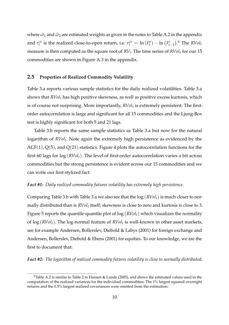
2.5 Properties of Realized Commodity Volatility

Table 3.a reports various sample statistics for the daily realized volatilities. Table 3.a

shows that RVolt has high positive skewness, as well as positive excess kurtosis, which

is of course not surprising. More importantly, RVolt is extremely persistent. The first-

order autocorrelation is large and significant for all 15 commodities and the Ljung-Box

test is highly significant for both 5 and 21 lags.

Table 3.b reports the same sample statistics as Table 3.a but now for the natural

logarithm of RVolt. Note again the extremely high persistence as evidenced by the

ACF(1), Q(5), and Q(21) statistics. Figure 4 plots the autocorrelation functions for the

first 60 lags for log (RVolt). The level of first-order autocorrelation varies a bit across

commodities but the strong persistence is evident across our 15 commodities and we

can write our first stylized fact:


Comparing Table 3.b with Table 3.a we also see that the log (RVolt) is much closer to nor-

mally distributed than is RVolt itself; skewness is close to zero and kurtosis is close to 3.

Figure 5 reports the quantile-quantile plot of log (RVolt) which visualizes the normality

of log (RVolt). The log-normal feature of RVolt is well-known in other asset markets,

see for example Andersen, Bollerslev, Diebold & Labys (2001) for foreign exchange and

Andersen, Bollerslev, Diebold & Ebens (2001) for equities. To our knowledge, we are the

first to document that:


6Table A.2 is similar to Table 2 in Hansen & Lunde (2005), and shows the estimated values used in thecomputation of the realized variances for the individual commodities. The 1% largest squared overnightreturns and the 0.5% largest realized covariances were omitted from the estimation.

10

Given the approximately normal distribution of log-realized volatility found in Table

3.b, we model the expected log (RVolt) and use an ARMA(1,1) specification, defined by

log(RVolt) = φ0 + φ1 log(RVolt−1) + θ1et−1 + et. (2)

We choose an ARMA(1,1) specification to capture the strong persistence in log (RVolt)

and also to capture the unavoidable measurement error in the realized variance measure

defined in equation 1 above.7 Table A.3.a in the appendix contains the ARMA-coefficient

estimates. Figure 6 contains time series plots of the expected one-day ahead log(RVolt)

computed as

Et−1[log(RVolt)] = φ0 + φ1 log(RVolt−1) + θ1et−1.

For comparison, we also plot the realized stock market volatility (in grey) using the

Spyder futures contract.8 Note that the commodity log (RVolt) - unlike the RVolt levels

- are fairly well-behaved over time and in some cases shows a slightly decreasing trend

over time. The concern of increased commodity market volatility often raised in the

popular press does therefore not appear to be warranted.

3 Factor Structure in Commodity Returns and Volatility

In this section we investigate the multivariate properties of commodity returns and

volatility. We pay particular attention to the factor structure in the cross-section of

commodities.

3.1 A Common Factor in Commodity Returns?

In order to get a quick first glance at the cross-commodity return dependence, the upper

triangle of the matrix in Table 4 reports the sample correlations for daily futures returns.

Note the high correlations for energy and metals, the somewhat lower correlations for

7Using a fractionally integrated ARFIMA(1, d, 1) model to capture the long memory in volatility doesnot change any of our conclusions nor does recursively estimating the ARMA(1,1) model.

8Figure A.4 in the appendix contains time series plots of the raw log (RVolt) series.

11

grains and softs, and the close-to-zero correlations for meats. The average correlation

with all other commodities is highest for light crude at 34% and lowest for lean hogs at

12%. The diversification benefits thus varies greatly across commodities. The average

correlation across all pairs of commodity returns is 25%.

We now investigate the evidence of a common factor in our 15 commodity returns.

Using the sample correlations in the upper triangle of Table 4, we compute the principal

components (PCs) for the 15 return series and in Figure 7.a we plot the cumulative return

for the first four PCs. The first four PCs explain 30%, 15%, 10%, and 7% respectively,

for a total of 62% of the cross-sectional variation in the 15 commodity futures returns.

Comparing the top-left panel in Figure 7.a with the top-left panel in Figure 1 we see that

the first PC appears to capture the 2007-08 run up, and subsequent crash in oil prices.

Table 5.a reports the regressions of each commodity on the first four PCs. For each

commodity we run a separate PC analysis based only on the other 14 commodities to

avoid endogeneity issues in these regressions. See from the R2 how all 15 commodities

load positively on the first PC. Note also that the first four factors explain much of the

variation in oil, metals and grains, much less so for softs, and virtually none for meats.

The average R2 across the 15 commodity return regressions is 23%. We conclude:


excluding meats.

3.2 A Common Factor in Commodity Volatility?

Our daily realized volatility measures computed from intraday returns allow us to view

volatility as an observed time series albeit measured with error. We therefore now inves-

tigate the multivariate properties of our 15 commodity log (RVt). The bottom triangle

of the matrix in Table 4 contains the sample correlations for log (RVolt). Note that the

correlations for log volatility is higher than for returns for all of the 15 commodities.

This is particularly the case for meats, where the average return correlation for live

cattle, lean hogs, and feeder cattle is 20%, 12%, and 14% respectively, whereas their

average log (RVolt) correlations are 52%, 48%, and 49%. The average correlation across

all pairs of commodity volatilities is 46% compared with 25% for returns.

12

The first four principal components corresponding to the ARMA(1,1) filtered log (RVolt)

are reported in Figure 7.b. The first four PCs capture 50%, 11%, 10%, and 6% respec-

tively, for a total of 77% of the total variation. Note again that the first PC for expected

log (RVolt) in the top left panel of Figure 7.b resembles quite closely the time series of

expected log (RVolt) for light crude in the top left panel of Figure 6.

Table 5.b reports the regressions of each expected log (RVolt) on the first four PCs.

For each commodity, we again run a separate PC analysis based only on the other

14 commodities to avoid endogeneity issues in these regressions. Note that all 15

commodities load positively on the first factor. Table 5.b also reports the regression fit,

R2, of each commodity. They show that the first four PCs capture a substantial share

of the variation for all commodities except perhaps coffee. The average R2 is 54% for

volatility compared with 23% for returns. Compared with the commonality in returns,

the commonality in volatility is much greater. We conclude:



3.3 Time-Varying Commodity Market Integration

It is natural to ask if the principal component analysis in Table 6 is stable over time. In a

study of international equity markets by Pukthuanthong & Roll (2009), they introduce a

measure of time-varying market integration which is based on a time-varying principal

component analysis. Following their approach we regress the return for each commodity

on the first 10 PCs computed separately for each year and computed using only the other

14 commodities.9 Using only daily returns within a given calendar year, the measure of

time-varying market integration of Pukthuanthong & Roll (2009) consists of the time

series of the annual adjusted R2 from these return regressions. While Pukthuanthong &

Roll (2009) only carry out the integration analysis on returns, we conduct their analysis

first for returns and then for expected log-realized volatility.

Our results are reported in Figure 8. The adjusted R2 from the return regressions are

shown with a black line and the adjusted R2 from the volatility regressions are shown

9Our results are robust when changing the number of PCs used.

13

in grey. Three important conclusions are obtained from Figure 8. First, the evidence

for commodity market integration is generally stronger when based on volatility than

when based on returns. This is especially true for livestock. Second, the degree of market

integration varies greatly by commodity. It is strongest for oil and metals. Third, there

is no obvious evidence of a time-trend in the degree of market integration during our

2004-2013 sample period. Indeed, the Pukthuanthong & Roll (2009) market integration

measure for returns decreased in 2013 for all commodities except gold and silver. Note

further that for several commodities the market appears to be less integrated in 2013

than in 2004 by this measure. We conclude:



4 The Stock Market as Factor for Commodity Returns and Volatility

In this section we study the extent to which daily commodity returns and volatilities

are integrated with equity market returns and volatilities. We use intraday trades on

the Spyder futures contract to compute realized stock market volatility as described in

Section 2 above. We then assess the ability of Spyder returns and realized volatility to

explain commodity futures and returns in comparison with the four principal compo-

nents used above. Finally, we construct realized covariance measures which enable us

to construct realized betas and realized systematic risk ratios.

4.1 Spyder as an Observed Factor for Commodity Returns and Volatility

The second to last line in Table 4 shows the sample correlation between Spyder returns

and the return of each commodity. The correlations range from 6% for lean hogs to 45%

for copper. The average correlation with Spyder returns is 22%. The last line in Table 4

shows the correlation between Spyder volatility and the volatility of each commodity.

The correlations are generally high with an average of 37%. They are highest for light

crude and the three metals. It is lowest for coffee and natural gas which are outliers

14

in this regard. The Spyder volatilities are plotted in grey along with each commodity

volatility in Figure 6.

In Table 5.a we assessed the ability of the first four principal components for the

commodities to explain the variation in returns and volatility over time. The principal

components can be viewed as unobserved factors and the obvious next step is to ask if

any observed factors can capture the variation in the PCs and thus in the commodity

returns and volatility? We now want to assess the ability of Spyder to serve as an

observed factor for the commodity futures market.

To this end we first regress each commodity PC on Spyder to obtain a Spyder-

orthogonalized PC series from the residuals. We then regress the return for each com-

modity on the Spyder return as well as on the four orthogonalized principal components.

Again, the PCs used for each commodity are constructed from the remaining 14 com-

modities only.

Table 6.a contains the results for returns. The results show that the Spyder return is

significant in all 15 commodity return regressions. The coefficient ranges from around

15% for livestock and gold to around more than 50% for the other metals and oil. The

average regression R2 is 24%.

In Table 6.b we report on regressions for expected realized volatility. Again, we first

orthogonalize each of the PC expected volatility factors with expected Spyder volatility.

Table 6.b shows that the Spyder coefficients are significant in 13 out of 15 cases. The

exceptions are natural gas and coffee. The average R2 is 55%.

Consider finally the sample correlation between Spyder volatility and the first four

commodity volatility PCs plotted in Figure 7.b. The four correlations are65%, 32%, −2%,

and −20% respectively (not reported in the tables). This shows that the most important

factor for commodity volatility is very highly correlated with stock market volatility,

and we can write:


volatility.

15

4.2 Constructing Realized Covariance Measures

Our next task is to compute daily realized covariance measures for each commodity

with Spyder. The ultimate goal is to compute stock market betas for each commodity

that vary daily without imposing a particular dynamic model a priori.

For the bivariate analysis with Spyder, overlapping trading spans between commod-

ity i and Spyder is required to avoid a bias towards zero in the realized covariances.

Therefore, opening and closing prices are now redefined as the most recently observed

price before the start and end of the overlapping trading span between commodity i and

Spyder, respectively. This is illustrated by the grey shading in Figure 3. Spyder trades on

NASDAQ from 9.30 to 16.00 in the full sample period, but for commodities the futures

trading spans have changed several times. Therefore, the overlapping trade spans varies

across commodities and over time. See Table A.4 in the appendix for details.

The construction of realized covariances is similar to the construction of the realized

variances above. Within overlapping trade spans, a synchronised 1-minute time-grid

between the commodities and Spyder is constructed. From the synchronised prices,

1-minute log-returns on day t are calculated. Then, using overlapping 5-minute returns

as in Section 2.4, the realized covariance with 1-minute subsampling is for commodity i

calculated as,

RCovoci,t =

n(i)n(i)− 4

· 15

n(i)−4

∑k=1

r(k)i,t r(k)SPY,t,

where we again use a rescaling to make sure the realized covariance estimate is unbiased.

The subsampling technique is used to eliminate bias from market microstructure noise

and non-synchronous trades within the overlapping trading span, see e.g. Barndorff-

Nielsen & Shephard (2004).

Finally, realized variance and covariance measures are matched to close-close returns

following Hansen & Lunde (2005). That is, the realized covariance matrix for the whole

day based on intermittent high-frequency data is for commodity i and Spyder given by

RCovi,t = ω1rcoi,tr

coSPY,t + ω2RCovoc

i,t, (3)

16

where rcoi,t and rco

SPY,t is the realized close-to-open return, e.g. rcoi,t = ln

(Fo

i,t

)− ln

(Fc

i,t−1

),

for commodity i and Spyder respectively, and ω1 and ω2 are again estimated weights

similar to the ones reported for the univariate case in Table A.2 in the appendix.

4.3 Realized Spyder Betas for Commodities

We now investigate the ability of the stock market to explain the variation in returns on

the 15 commodity futures contracts. Recognizing that the relationship between each

commodity and the stock market is likely changing over time, we follow Andersen,

Bollerslev, Diebold & Wu (2005) and Patton & Verardo (2012) who use intraday data to

compute a daily model-free realized beta for each asset defined by

Rβi,t =RCovi,t

RVSPY,t. (4)

The realized covariance, RCovi,t, is calculated on the cross-product of the intraday

commodity and stock market return using the estimator in equation 3.

In order to filter the realized betas in equation 4 we estimate an ARMA(1,1) on each

realized beta series. The time series of the filtered betas are plotted in Figure 9 and

the ARMA coefficients are reported in Table A.3.b in the appendix. The appendix also

contains a plot of the raw realized betas in Figure A.5.

We plot the beta series along with bootstrapped 75% and 90% confidence intervals

constructed by resampling with replacement from the ARMA residuals. The confidence

intervals are based on 10, 000 bootstrap samples.

Figure 9 shows that the realized betas were close to zero until 2008, then rose

dramatically in many cases to and even beyond one. The decrease in commodity betas

since 2010 are equally interesting. By the end of 2013 all the realized betas were back to

zero, the level at which they began at the onset of financialization in 2004. The betas

were highest for energy and metals. The remarkable rise and fall of the commodity

betas are shared by all except for lean hogs and feeder cattle which stayed close to zero

throughout the period. We assert:



17

The beta of an asset does not tell us how much of the variance in the asset’s return is

driven by the market factor. To this end we define the Systematic Risk Ratio (SRR) for

commodity i by

SSRi,t =Rβ2

i,t · RVSPY,t

RVi,t. (5)

The SSR can thus be interpreted as the fraction of commodity i variance that is explained

by market variance. Clearly, 0 ≤ SSRi,t ≤ 1. Our use of high-frequency data enables us

to compute a systematic risk ratio for each commodity on each day. We again estimate

an ARMA(1,1) on the raw SRR to filter the series. The ARMA coefficients and the raw

SRR series are provided in the appendix. Figure 10 plots the time series of the filtered

SRR along with the average SRR over the sample period with bootstrapped 75% and

90% confidence intervals for the ARMA residuals. Note how the SRR was close to zero

for all commodities before 2008, it then rose to substantial levels - in particular for

energy and metals - before returning to zero at the end of 2013.

4.4 Capturing Nonlinear Dependence with Spyder

So far we have focused on linear dependence between commodity futures and the stock

market. In this section we investigate nonlinear relationships.

Figure 11 shows the threshold correlations for each daily commodity futures returns

versus the daily return on the stock index ETF. Threshold correlations are computed as

ρij(u) =

Corr(ri, rj

∣∣ri < Fi-¹(u) and rj < Fj

-¹(u))

if u < 0.5

Corr(ri, rj

∣∣ri ≥ Fi-¹(u) and rj ≥ Fj

-¹(u))

if u ≥ 0.5,

where u is a threshold between 0 and 1, and Fi−1(u) is the empirical quantile of the

univariate distribution of ri. The horizontal axis in Figure 11 denotes the percentile used

to define each threshold for the correlation on the vertical axis. We only compute the

threshold correlation when at least 60 observations are available, and again we perform

the calculations with (black lines) and without (grey lines) rollover returns.

The dashed lines in Figure 11 denotes the threshold correlation from a bivariate

18

normal distribution with a correlation equal to the sample correlation from the futures

data. Figure 11 shows that the deviation from bivariate normality is large for oil, all

metals, and for some of the agriculturals as well. While the simple linear correlations can

be small, the threshold correlations are often large. It is important to keep in mind that

the threshold correlations are unconditional - they are computed once from the entire

sample. Figure 9 above showed that the stock market exposure of each commodity

varies greatly over time. This dynamic beta may be the cause of the large threshold

correlations we see in Figure 11.

We next compute threshold correlations for the expected log (RVolt) for each com-

modity versus log (RVolt) in Spyder. They are plotted in Figure 12 which shows that

large positive shocks to volatility in the stock market are generally highly correlated

with large positive shocks to the volatility of each commodity. This is particularly true

for oil and metals but also for most of the agriculturals.

5 The Distribution of Commodity Returns and Shocks

So far, we have focused on the dependence structure across commodity futures returns

and volatilities. To obtain a fully specified model, we need to make distributional

assumptions as well. We therefore now investigate the distribution of futures returns

and the extent to which standardizing the daily commodity futures returns by expected

realized volatility will produce a close to normally distributed series of commodity

futures shocks.

5.1 The Distribution of Commodity Futures Returns

As mentioned above, Table 2.a reports various sample statistics for the daily log returns

on our 15 commodity futures. During our 2004-2013 sample period, the average log

return was highest for silver at 4.7 bps per day and lowest for natural gas at −1.5 bps

per day. Heating oil, copper, gold, and light crude appreciated strongly during the

sample as well. Natural gas had by far the highest average daily volatility at more than

3.3% per day compared with feeder cattle which only had a volatility of less than 1%

19

per day. These findings also hold when the rollover returns are removed. We note that

the cross-commodity variation in commodity return mean and volatility is large.

Table 2.a also provides information on the unconditional distribution of daily returns.

Cotton contains by far the largest negative daily return at −39.3%, which is a 19 standard

deviation move that occurred on February 16, 2011. This corresponds to a rollover return.

Lean hogs has the largest positive daily return at 25.9% which also corresponds to a

rollover return. However, even with rollovers removed, the minimum and maximum

observations for all commodities are quite extreme; perhaps with the exception of live

and feeder cattle. Not surprisingly, given the extreme minimum value, cotton has the

largest negative skewness at −2.5. Lean hogs has the highest positive skewness at 2.0.

The cross-sectional range in skewness is thus large. Kurtosis is in excess of the Gaussian

value of 3 for all 15 commodities. It is not surprisingly largest at 54.2 for cotton whereas

coffee has the lowest value at 3.9. Results are very different for both skewness and

kurtosis for most commodities when rollover returns are removed. In this case, silver is

the commodity with both the largest (negative) skewness and kurtosis. These findings

are not surprising because sample estimates of skewness and kurtosis are well-known

to be heavily influenced by a few large outlying observations, see Kim & White (2004).

Figure A.6 in the appendix reports QQ plots against the normal distribution which

provides further evidence on the non-normality of raw returns and the important

impact on the tail of the distribution from roll-returns. For now, we simply note that the

unconditional distribution of commodity returns is highly leptokurtotic with substantial

variation in skewness across commodities.

5.2 Commodity Futures Shocks

If we assume that et is i.i.d. normally distributed, which is sensible given Table 3.b,

then we can use the moment-generating function of a normal variable to construct our

measure of expected RVolt, as

Et−1[RVolt] = exp [Et−1[log(RVolt)]] · exp[

12

σ2e

],

20

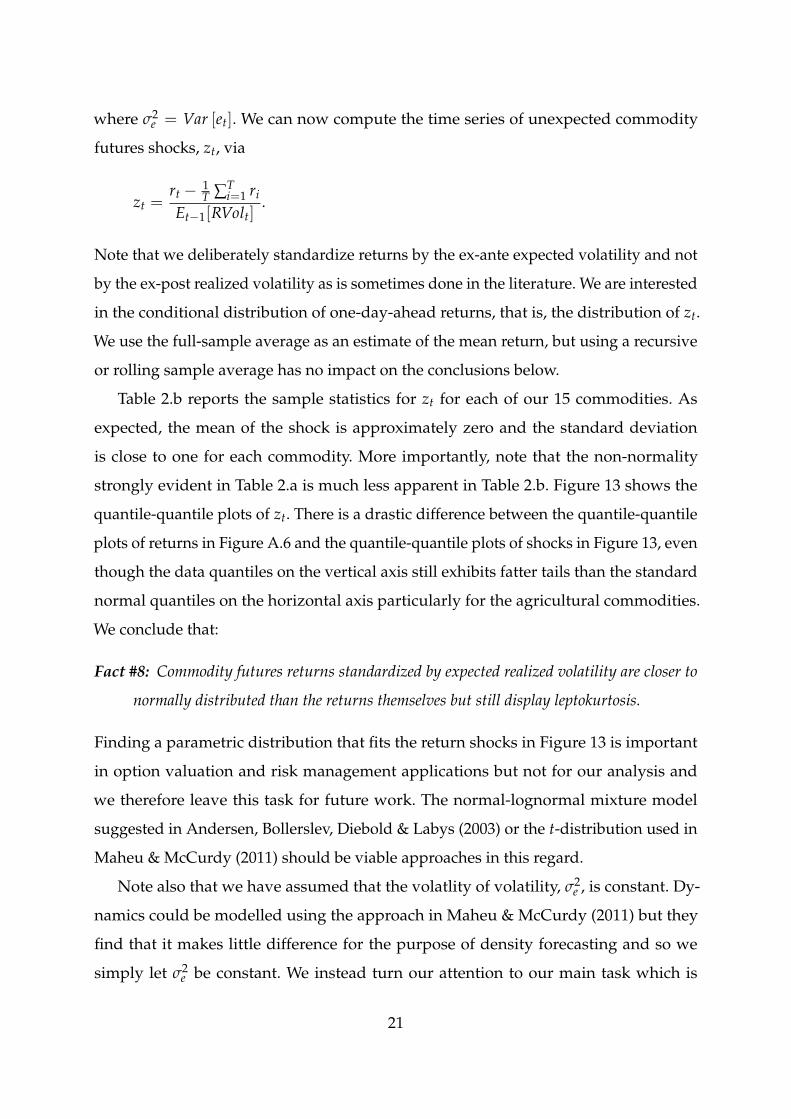
where σ2e = Var [et]. We can now compute the time series of unexpected commodity

futures shocks, zt, via

zt =rt − 1

T ∑Ti=1 ri

Et−1[RVolt].

Note that we deliberately standardize returns by the ex-ante expected volatility and not

by the ex-post realized volatility as is sometimes done in the literature. We are interested

in the conditional distribution of one-day-ahead returns, that is, the distribution of zt.

We use the full-sample average as an estimate of the mean return, but using a recursive

or rolling sample average has no impact on the conclusions below.

Table 2.b reports the sample statistics for zt for each of our 15 commodities. As

expected, the mean of the shock is approximately zero and the standard deviation

is close to one for each commodity. More importantly, note that the non-normality

strongly evident in Table 2.a is much less apparent in Table 2.b. Figure 13 shows the

quantile-quantile plots of zt. There is a drastic difference between the quantile-quantile

plots of returns in Figure A.6 and the quantile-quantile plots of shocks in Figure 13, even

though the data quantiles on the vertical axis still exhibits fatter tails than the standard

normal quantiles on the horizontal axis particularly for the agricultural commodities.

We conclude that:



Finding a parametric distribution that fits the return shocks in Figure 13 is important

in option valuation and risk management applications but not for our analysis and

we therefore leave this task for future work. The normal-lognormal mixture model

suggested in Andersen, Bollerslev, Diebold & Labys (2003) or the t-distribution used in

Maheu & McCurdy (2011) should be viable approaches in this regard.

Note also that we have assumed that the volatlity of volatility, σ2e , is constant. Dy-

namics could be modelled using the approach in Maheu & McCurdy (2011) but they

find that it makes little difference for the purpose of density forecasting and so we

simply let σ2e be constant. We instead turn our attention to our main task which is

21

uncovering the stylized fact of the joint distribution of commodity futures returns as

well as of their volatilities.

Figure A.7 in the appendix shows the threshold correlations for the return shocks,

zt. Note that they are very close to zero for all commodities except coffee. Coffee is

clearly affected by rollover returns, but is also the only commodity with periodicity in

volatility as it is evident from Figure 5. Comparing Figure 11 with Figure A.7 suggests

that the large threshold correlations in returns are driven by time-varying volatility,

so that when dynamically standardized, commodity returns show little evidence of

significant threshold correlations.

6 Conclusion

We have addressed the following questions:

First, what are the stylized facts of commodity futures returns and volatility post

financialization? Second, is there a factor structure in commodity futures returns? Third,

is the stock market driving the common component of commodity futures returns?

Fourth, do the stock market betas of commodity futures returns vary significantly over

time? Fifth, does the ratio of commodity futures return volatility explained by the

stock market beta change over time? Sixth, is there a factor structure in commodity

futures volatility? Finally, is stock market volatility driving the common component of

commodity futures volatility?

Analyzing almost a billion trades on 15 commodity futures contracts for the 2004-

2013 period, we have uncovered the following:




excluding meats.



22




volatility.





An appropriate option valuation model or portfolio risk model for commodity futures

needs to incorporate these features. We have deliberately taken a model-free approach

in this paper. But our results suggest that the parametric models developed in Andersen

et al. (2003) and Maheu & McCurdy (2011) present viable approaches.

Our results also show that the fear of increased volatility in the commodity markets

as a consequence of financialization is largely overblown. Commodity volatility has

not trended up nor has commodity return covariance with the stock market trended

up. Commodity returns are not riskier now than a decade ago and commodities do not

appear to have lost their ability to diversify equity market exposure.

Finally, our results have important implications for understanding the cross-section

of commodity futures returns. In recent work focusing on the U.S. equity market, Chen

& Petkova (2012), Duarte, Kamara, Siegel & Sun (2014), and Herskovic, Kelly, Lustig &

Van Nieuwerburgh (2014) find very strong evidence of factor structure in idiosyncratic

volatility. We find the same to be true in commodity futures volatility. Developing an

asset pricing framework that can capture this feature presents an important challenge

for future work.

23

References

Andersen, T., Bollerslev, T., Christoffersen, P. & Diebold, F. (2013), Financial risk mea-

surement for financial risk management, in G. Constantinides, M. Harris & R. Stulz,

eds, ‘Handbook of the Economics of Finance’, Vol. 2B, Elsevier, pp. 1127–1220.

Andersen, T. G., Bollerslev, T., Diebold, F. X. & Ebens, H. (2001), ‘The distribution of

realized stock return volatility’, Journal of Financial Economics 61(1), 43–76.

Andersen, T. G., Bollerslev, T., Diebold, F. X. & Labys, P. (2001), ‘The distribution of

exchange rate volatility’, Journal of the American Statistical Association 96(453), 42–55.

Correction published in 2003, volume 98, page 501.

Andersen, T. G., Bollerslev, T., Diebold, F. X. & Labys, P. (2003), ‘Modeling and forecast-

ing realized volatility’, Econometrica 71(2), 579–625.

Andersen, T. G., Bollerslev, T., Diebold, F. X. & Wu, J. (2005), ‘A framework for explor-

ing the macroeconomic determinants of systematic risk’, American Economic Review

95(2), 398–404.

Ang, A. & Chen, J. (2002), ‘Asymmetric correlations of equity portfolios’, Journal of

Financial Economics 63(3), 443–494.

Ang, A., Hodrick, R. J., Xing, Y. & Zhang, X. (2006), ‘The cross-section of volatility and

expected returns’, Journal of Finance 61(1), 259–299.

Ang, A., Hodrick, R. J., Xing, Y. & Zhang, X. (2009), ‘High idiosyncratic volatility and

low returns: International and further U.S. evidence’, Journal of Financial Economics

91(1), 1–23.

Baker, S. D. (2014), The financialization of storable commodities, Working paper, Uni-

versity of Virginia.

Baker, S. D. & Routledge, B. (2012), The price of oil risk, Working paper, Carnegie Mellon

University.

24

Bakshi, G., Gao, X. & Rossi, A. (2013), Asset pricing models that explain the cross-section

and time-series of commodity returns, Working paper, University of Maryland.

Barndorff-Nielsen, O. E., Hansen, P. R., Lunde, A. & Shephard, N. (2009), ‘Realised

kernels in practice: Trades and quotes’, Econometrics Journal 12, C1–C32.

Barndorff-Nielsen, O. E. & Shephard, N. (2004), ‘Econometric analysis of realised co-

variation: High frequency based covariance, regression and correlation in financial

economics’, Econometrica 72, 885–925.

Barndorff-Nielsen, O. E. & Shephard, N. (2007), Variation, jumps and high frequency

data in financial econometrics, in R. Blundell, T. Persson & W. K. Newey, eds, ‘Ad-

vances in Economics and Econometrics. Theory and Applications, Ninth World

Congress’, Econometric Society Monographs, Cambridge University Press, pp. 328–

372.

Basak, S. & Pavlova, A. (2014), A model of financialization of commodities, Working

paper, London Business School.

Bekaert, G., Harvey, C. R., Lundblad, C. T. & Siegel, S. (2011), ‘What Segments Equity

Markets?’, Review of Financial Studies 24(12), 3841–3890.

Bessembinder, H. (1992), ‘Systematic risk, hedging pressure, and risk premiums in

futures markets’, Review of Financial Studies 5(4), 637–67.

Bessembinder, H. & Chan, K. (1992), ‘Time-varying risk premia and forecastable returns

in futures markets’, Journal of Financial Economics 32(2), 169–193.

Boons, M., Roon, F. & Szymanowska, M. (2013), ‘The stock market price of commodity

risk’, Working paper, Tilburg University .

Büyüksahin, B., Haigh, M. S. & Robe, M. A. (2010), ‘Commodities and equities: A

"market of one"?’, Journal of Alternative Investments 12.

Carrieri, F., Errunza, V. & Hogan, K. (2007), ‘Characterizing world market integration

through time’, Journal of Financial and Quantitative Analysis 42, 915–940.

25

Chen, Z. & Petkova, R. (2012), ‘Does idiosyncratic volatility proxy for risk exposure?’,

Review of Financial Studies 25(9), 2745–2787.

Cheng, I.-H. & Xiong, W. (2013), The financialization of commodity markets, NBER

working papers, National Bureau of Economic Research, Inc.

Daskalaki, C., Kostakis, A. & Skiadopoulos, G. (2014), ‘Are there common factors in

individual commodity futures returns?’, Journal of Banking & Finance 40(C), 346–363.

Duarte, J., Kamara, A., Siegel, S. & Sun, C. (2014), ‘The systematic risk of idiosyncratic

volatility’, SSRN Working Paper .

Engle, R. F. (2002), ‘Dynamic conditional correlation - a simple class of multivariate

GARCH models,’, Journal of Business & Economic Statistics 20(3), 339–350.

Gorton, G. B., Hayashi, F. & Rouwenhorst, G. K. (2012), ‘The fundamentals of commodity

futures returns’, Yale ICF Working paper No. 07-08.

Gorton, G. & Rouwenhorst, K. G. (2006), ‘Facts and fantasies about commodity futures’,

Financial Analysts Journal pp. 47–68.

Hamilton, J. D. & Wu, J. C. (2014), Effects of index-fund investing on commodity futures

prices, NBER working paper, National Bureau of Economic Research, Inc.

Hansen, P. R. & Lunde, A. (2005), ‘A realized variance for the whole day based on

intermittent high-frequency data’, Journal of Financial Econometrics 3, 525–544.

Hansen, P. R. & Lunde, A. (2011), Forecasting volatility using high-frequency data, in

M. Clements & D. Hendry, eds, ‘The Oxford Handbook of Economic Forecasting’,

Oxford: Blackwell, chapter 19, pp. 525–556.

Henderson, B., Pearson, N. & Wang, L. (2013), New evidence on the financialization of

commodity markets, Working paper, University of Illinois at Urbana-Champaign.

Herskovic, B., Kelly, B., Lustig, H. & Van Nieuwerburgh, S. (2014), The common factor

in idiosyncratic volatility: Quantitative asset pricing implications, Working paper,

University of Chicago, Booth School of Business.

26

Kim, T.-H. & White, H. (2004), ‘On more robust estimation of skewness and kurtosis’,

Finance Research Letters 1(1), 56–73.

Longin, F. & Solnik, B. (2001), ‘Extreme correlation of international equity markets’, The

Journal of Finance 56(2), 649–676.

Maheu, J. M. & McCurdy, T. H. (2011), ‘Do high-frequency measures of volatility im-

prove forecasts of return distributions?’, Journal of Econometrics 160(1), 69–76.

Patton, A. J. & Verardo, M. (2012), ‘Does beta move with news? firm-specific information

flows and learning about profitability’, Review of Financial Studies 25(9), 2789–2839.

Pukthuanthong, K. & Roll, R. (2009), ‘Global market integration: An alternative measure

and its application’, Journal of Financial Economics 94(2), 214–232.

Singleton, K. J. (2014), ‘Investor flows and the 2008 boom/bust in oil prices’, Management

Science 60(2), 300–318.

Szymanowska, M., De Roon, F., Nijman, T. & Van Den Goorbergh, R. (2014), ‘An anatomy

of commodity futures risk premia’, The Journal of Finance 69(1), 453–482.

Tang, K. & Xiong, W. (2012), ‘Index investment and financialization of commodities’,

Financial Analysts Journal 68, 54–74.

Zhang, L., Mykland, P. A. & Aït-Sahalia, Y. (2005), ‘A tale of two time scales: Determining

integrated volatility with noisy high frequency data’, Journal of the American Statistical

Association 100, 1394–1411.

27

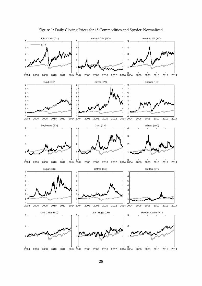
Figure 1: Daily Closing Prices for 15 Commodities and Spyder. Normalized.

2004 2006 2008 2010 2012 20140

1

2

3

4

5Light Crude (CL)

SPY

2004 2006 2008 2010 2012 20140

1

2

3

4

5Natural Gas (NG)

2004 2006 2008 2010 2012 20140

1

2

3

4

5Heating Oil (HO)

2004 2006 2008 2010 2012 20140

1

2

3

4

5

6

7

8Gold (GC)

2004 2006 2008 2010 2012 20140

1

2

3

4

5

6

7

8Silver (SV)

2004 2006 2008 2010 2012 20140

1

2

3

4

5

6

7

8Copper (HG)

2004 2006 2008 2010 2012 20140

1

2

3

4Soybeans (SY)

2004 2006 2008 2010 2012 20140

1

2

3

4Corn (CN)

2004 2006 2008 2010 2012 20140

1

2

3

4Wheat (WC)

2004 2006 2008 2010 2012 20140

1

2

3

4

5

6

7Sugar (SB)

2004 2006 2008 2010 2012 20140

1

2

3

4

5

6

7Coffee (KC)

2004 2006 2008 2010 2012 20140

1

2

3

4

5

6

7Cotton (CT)

2004 2006 2008 2010 2012 20140

1

2

3Live Cattle (LC)

2004 2006 2008 2010 2012 20140

1

2

3Lean Hogs (LH)

2004 2006 2008 2010 2012 20140

1

2

3Feeder Cattle (FC)

28

Figure 2: Number of Ticks, Volume and Dollar Volume for 15 Commodities. Annual Averages.

2004 2006 2008 2010 2012 20140.0

0.1

0.3

1.0

3.2Light Crude (CL)× 105 × 107

0.1

0.3

1.0

3.2

TicksVolumeDollar Volume

2004 2006 2008 2010 2012 2014 0.0

0.1

0.3

1.0

3.2

10.0Natural Gas (NG)× 104 × 105

0.3

1.0

3.2

10.0

2004 2006 2008 2010 2012 20140.0

0.1

0.3

1.0

3.2Heating Oil (HO)× 104 × 104

0.1

0.3

1.0

3.2

10.0

2004 2006 2008 2010 2012 20140.0

0.1

0.3

1.0

Gold (GC)× 105 × 108

0.0

0.1

0.3

1.0

3.2

2004 2006 2008 2010 2012 2014 0.0

0.1

0.3

1.0

3.2

10.0Silver (SV)× 104 × 106

0.0

0.1

0.3

1.0

3.2

2004 2006 2008 2010 2012 2014 0.0

0.1

0.3

1.0

3.2

10.0Copper (HG)× 104 × 105

0.0

0.1

0.3

1.0

3.2

2004 2006 2008 2010 2012 2014 0.0

0.1

0.3

1.0

3.2

10.0Soybeans (SY)× 104 × 106

0.0

0.1

0.3

1.0

3.2

2004 2006 2008 2010 2012 2014

0.0

0.1

0.3

1.0

Corn (CN)× 105 × 105

0.0

0.1

0.3

1.0

3.2

10.0

2004 2006 2008 2010 2012 2014 0.0

0.1

0.3

1.0

3.2

10.0Wheat (WC)× 104 × 105

0.0

0.1

0.3

1.0

3.2

2004 2006 2008 2010 2012 2014 0.0

0.1

0.3

1.0

3.2

10.0Sugar (SB)× 104 × 105

0.0

0.1

0.3

1.0

3.2

10.0

2004 2006 2008 2010 2012 20140.0

0.1

0.3

1.0

Coffee (KC)× 104 × 106

0.0

0.1

0.3

1.0

3.2

2004 2006 2008 2010 2012 20140.0

0.1

0.3

1.0

Cotton (CT)× 104 × 105

0.0

0.1

0.3

1.0

3.2

10.0

2004 2006 2008 2010 2012 20140.0

0.1

0.3

1.0

Live Cattle (LC)× 104 × 104

0.0

0.1

0.3

1.0

3.2

2004 2006 2008 2010 2012 20140.0

0.1

0.3

1.0

Lean Hogs (LH)× 104 × 104

0.0

0.1

0.3

1.0

3.2

2004 2006 2008 2010 2012 20140.0

0.1

0.3

1.0

3.2Feeder Cattle (FC)× 103 × 103

0.0

0.1

0.3

1.0

3.2

10.0

Notes: Ticks (left axis) denote the number of transactions, which may consist of one or more futurescontracts (pit and electronic). Volume (left axis) denotes the number of futures contracts traded (electroniconly), Dollar Volume (right axis) denotes the dollar value of the futures contracts traded using the closingprice each day (electronic only).

29

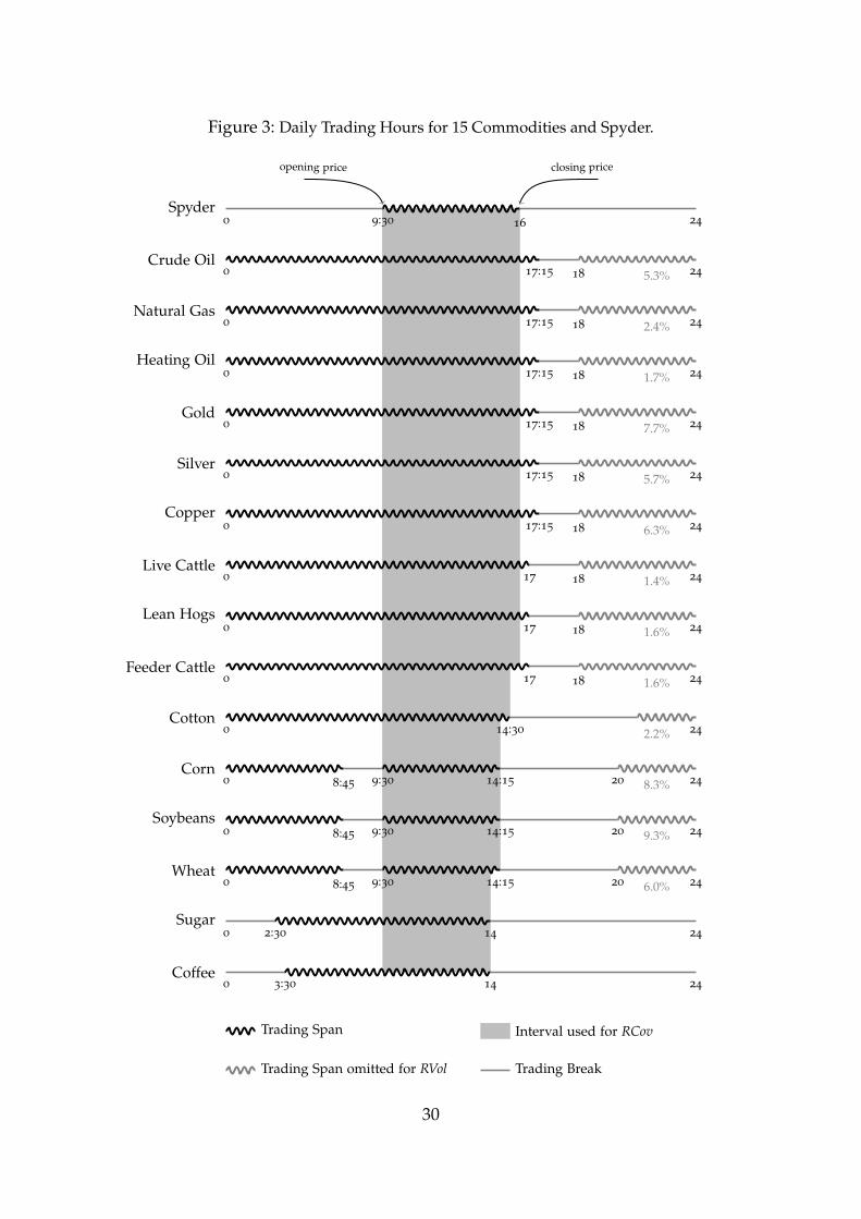
Figure 3: Daily Trading Hours for 15 Commodities and Spyder.

opening price closing price

Spyder0 9:30 16 24

Crude Oil0 17:15 18 245.3%

Natural Gas0 17:15 18 242.4%

Heating Oil0 17:15 18 241.7%

Gold0 17:15 18 247.7%

Silver0 17:15 18 245.7%

Copper0 17:15 18 246.3%

Live Cattle0 17 18 241.4%

Lean Hogs0 17 18 241.6%

Feeder Cattle0 17 18 241.6%

Cotton0 14:30 242.2%

Corn0 8:45 9:30 14:15 20 248.3%

Soybeans0 8:45 9:30 14:15 20 249.3%

Wheat0 8:45 9:30 14:15 20 246.0%

Sugar0 2:30 14 24

Coffee0 3:30 14 24

Trading Span

Trading Span omitted for RVol Trading Break

Interval used for RCov

30

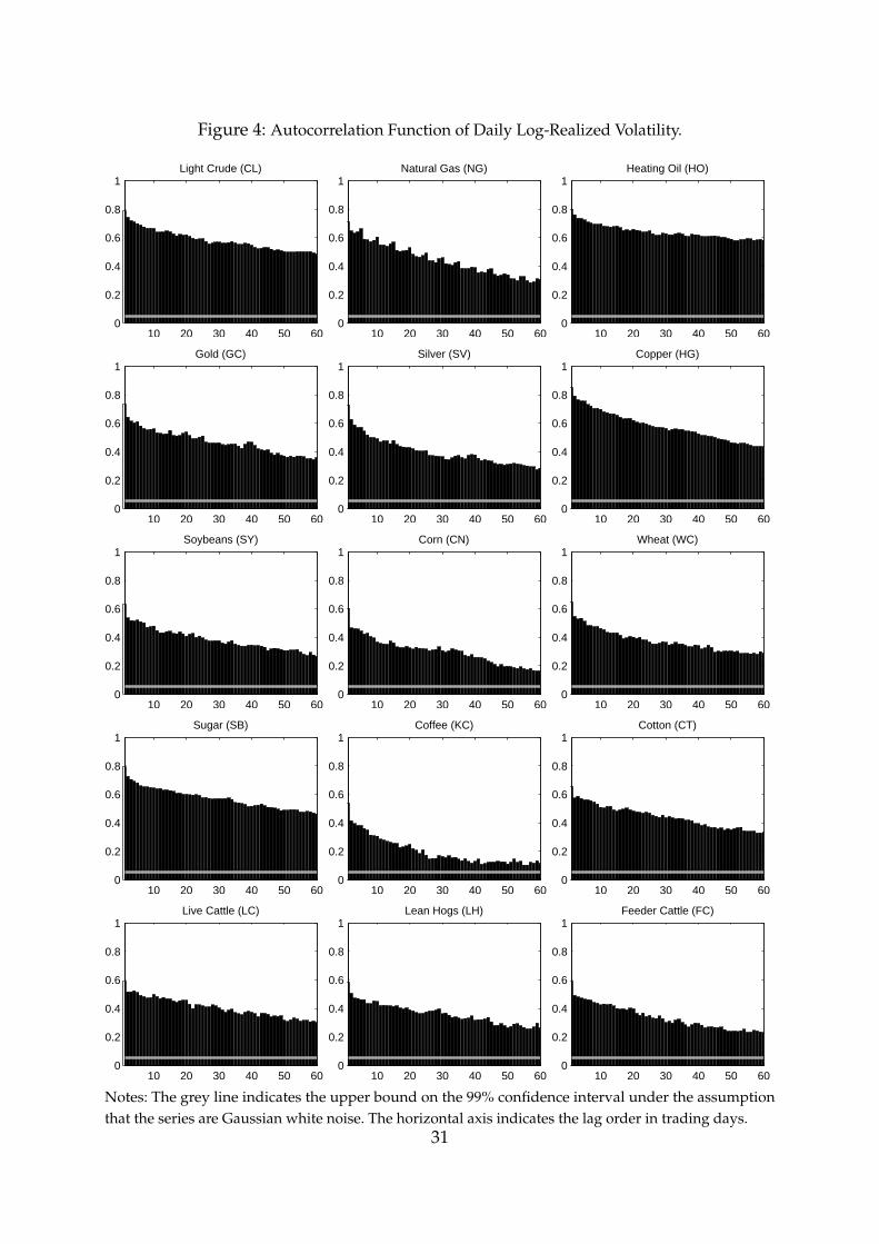
Figure 4: Autocorrelation Function of Daily Log-Realized Volatility.

10 20 30 40 50 600

0.2

0.4

0.6

0.8

1Light Crude (CL)

10 20 30 40 50 600

0.2

0.4

0.6

0.8

1Natural Gas (NG)

10 20 30 40 50 600

0.2

0.4

0.6

0.8

1Heating Oil (HO)

10 20 30 40 50 600

0.2

0.4

0.6

0.8

1Gold (GC)

10 20 30 40 50 600

0.2

0.4

0.6

0.8

1Silver (SV)

10 20 30 40 50 600

0.2

0.4

0.6

0.8

1Copper (HG)

10 20 30 40 50 600

0.2

0.4

0.6

0.8

1Soybeans (SY)

10 20 30 40 50 600

0.2

0.4

0.6

0.8

1Corn (CN)

10 20 30 40 50 600

0.2

0.4

0.6

0.8

1Wheat (WC)

10 20 30 40 50 600

0.2

0.4

0.6

0.8

1Sugar (SB)

10 20 30 40 50 600

0.2

0.4

0.6

0.8

1Coffee (KC)

10 20 30 40 50 600

0.2

0.4

0.6

0.8

1Cotton (CT)

10 20 30 40 50 600

0.2

0.4

0.6

0.8

1Live Cattle (LC)

10 20 30 40 50 600

0.2

0.4

0.6

0.8

1Lean Hogs (LH)

10 20 30 40 50 600

0.2

0.4

0.6

0.8

1Feeder Cattle (FC)

Notes: The grey line indicates the upper bound on the 99% confidence interval under the assumptionthat the series are Gaussian white noise. The horizontal axis indicates the lag order in trading days.

31

Figure 5: QQ-Plot of Daily Log-Realized Volatility.

−4 −2 0 2 4−4

−2

0

2

4

Std. Normal Quantiles

Dat

a Q

uant

iles

Light Crude (CL)

−4 −2 0 2 4−4

−2

0

2

4

Std. Normal QuantilesD

ata

Qua

ntile

s

Natural Gas (NG)

−4 −2 0 2 4−4

−2

0

2

4


Dat

a Q

uant

iles

Heating Oil (HO)

−4 −2 0 2 4−4

−2

0

2

4


Dat

a Q

uant

iles

Gold (GC)

−4 −2 0 2 4−4

−2

0

2

4


Dat

a Q

uant

iles

Silver (SV)

−4 −2 0 2 4−4

−2

0

2

4


Dat

a Q

uant

iles

Copper (HG)

−4 −2 0 2 4−4

−2

0

2

4


Dat

a Q

uant

iles

Soybeans (SY)

−4 −2 0 2 4−4

−2

0

2

4


Dat

a Q

uant

iles

Corn (CN)

−4 −2 0 2 4−4

−2

0

2

4


Dat

a Q

uant

iles

Wheat (WC)

−4 −2 0 2 4−4

−2

0

2

4


Dat

a Q

uant

iles

Sugar (SB)

−4 −2 0 2 4−4

−2

0

2

4


Dat

a Q

uant

iles

Coffee (KC)

−4 −2 0 2 4−4

−2

0

2

4


Dat

a Q

uant

iles

Cotton (CT)

−4 −2 0 2 4−4

−2

0

2

4


Dat

a Q

uant

iles

Live Cattle (LC)

−4 −2 0 2 4−4

−2

0

2

4


Dat

a Q

uant

iles

Lean Hogs (LH)

−4 −2 0 2 4−4

−2

0

2

4


Dat

a Q

uant

iles

Feeder Cattle (FC)

Notes: All observations are marked by dots. Crosses indicate large quantiles that do not correspond torollover returns.

32

Figure 6: Daily Expected Log-Realized Volatility.

2004 2006 2008 2010 2012 2014−2

−1

0

1

2Light Crude (CL)

SPY

2004 2006 2008 2010 2012 2014−2

−1

0

1

2Natural Gas (NG)

2004 2006 2008 2010 2012 2014−2

−1

0

1

2Heating Oil (HO)

2004 2006 2008 2010 2012 2014−2

−1

0

1

2Gold (GC)

2004 2006 2008 2010 2012 2014−2

−1

0

1

2Silver (SV)

2004 2006 2008 2010 2012 2014−2

−1

0

1

2Copper (HG)

2004 2006 2008 2010 2012 2014−2

−1

0

1

2Soybeans (SY)

2004 2006 2008 2010 2012 2014−2

−1

0

1

2Corn (CN)

2004 2006 2008 2010 2012 2014−2

−1

0

1

2Wheat (WC)

2004 2006 2008 2010 2012 2014−2

−1

0

1

2Sugar (SB)

2004 2006 2008 2010 2012 2014−2

−1

0

1

2Coffee (KC)

2004 2006 2008 2010 2012 2014−2

−1

0

1

2Cotton (CT)

2004 2006 2008 2010 2012 2014−2

−1

0

1

2Live Cattle (LC)

2004 2006 2008 2010 2012 2014−2

−1

0

1

2Lean Hogs (LH)

2004 2006 2008 2010 2012 2014−2

−1

0

1

2Feeder Cattle (FC)

33

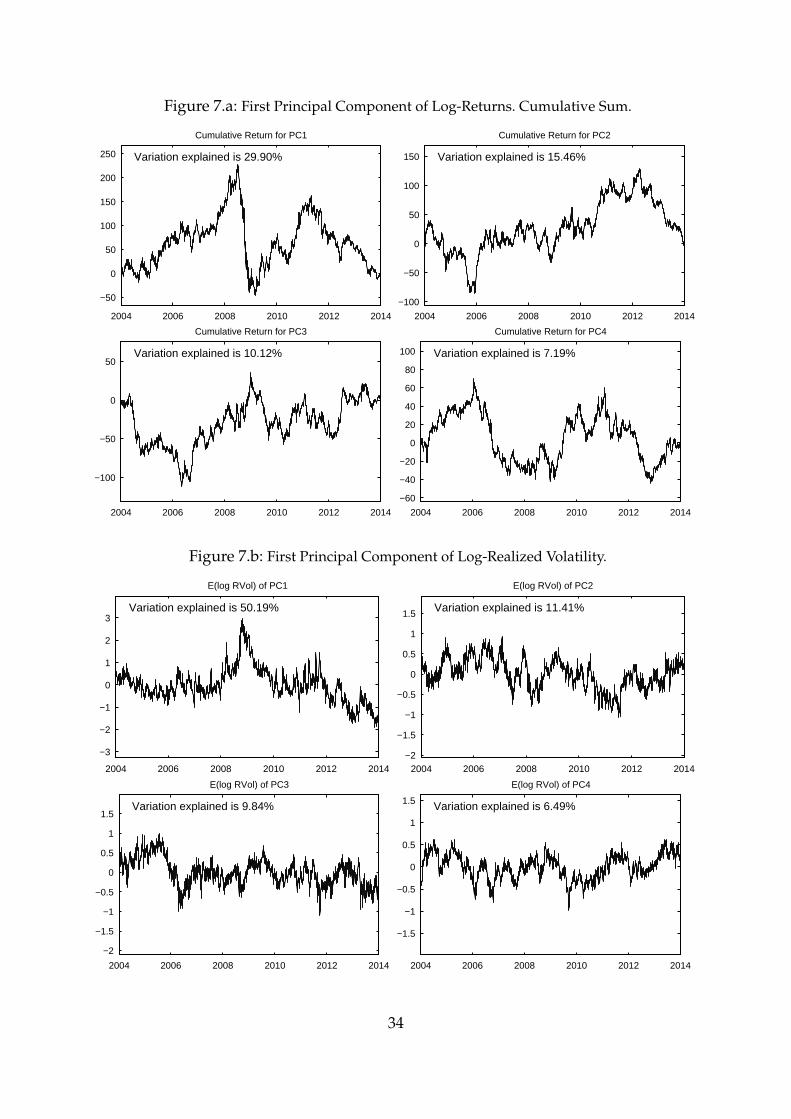
Figure 7.a: First Principal Component of Log-Returns. Cumulative Sum.

2004 2006 2008 2010 2012 2014

−50

0

50

100

150

200

250

Cumulative Return for PC1

Variation explained is 29.90%

2004 2006 2008 2010 2012 2014

−100

−50

0

50

100

150



2004 2006 2008 2010 2012 2014

−100

−50

0

50



2004 2006 2008 2010 2012 2014

−60

−40

−20

0

20

40

60

80

100



Figure 7.b: First Principal Component of Log-Realized Volatility.

2004 2006 2008 2010 2012 2014

−3

−2

−1

0

1

2

3

E(log RVol) of PC1


2004 2006 2008 2010 2012 2014−2

−1.5

−1

−0.5

0

0.5

1

1.5

E(log RVol) of PC2


2004 2006 2008 2010 2012 2014

−2

−1.5

−1

−0.5

0

0.5

1

1.5

E(log RVol) of PC3


2004 2006 2008 2010 2012 2014

−1.5

−1

−0.5

0

0.5

1

1.5

E(log RVol) of PC4


34

Figure 8: Time-Varying Market Integration in Returns and Volatility.

2004 2006 2008 2010 2012 20140

0.2

0.4

0.6

0.8

1Light Crude (CL)

ReturnsVolatility

2004 2006 2008 2010 2012 20140

0.2

0.4

0.6

0.8

1Natural Gas (NG)

2004 2006 2008 2010 2012 20140

0.2

0.4

0.6

0.8

1Heating Oil (HO)

2004 2006 2008 2010 2012 20140

0.2

0.4

0.6

0.8

1Gold (GC)

2004 2006 2008 2010 2012 20140

0.2

0.4

0.6

0.8

1Silver (SV)

2004 2006 2008 2010 2012 20140

0.2

0.4

0.6

0.8

1Copper (HG)

2004 2006 2008 2010 2012 20140

0.2

0.4

0.6

0.8

1Soybeans (SY)

2004 2006 2008 2010 2012 20140

0.2

0.4

0.6

0.8

1Corn (CN)

2004 2006 2008 2010 2012 20140

0.2

0.4

0.6

0.8

1Wheat (WC)

2004 2006 2008 2010 2012 20140

0.2

0.4

0.6

0.8

1Sugar (SB)

2004 2006 2008 2010 2012 20140

0.2

0.4

0.6

0.8

1Coffee (KC)

2004 2006 2008 2010 2012 20140

0.2

0.4

0.6

0.8

1Cotton (CT)

2004 2006 2008 2010 2012 20140

0.2

0.4

0.6

0.8

1Live Cattle (LC)

2004 2006 2008 2010 2012 20140

0.2

0.4

0.6

0.8

1Lean Hogs (LH)

2004 2006 2008 2010 2012 20140

0.2

0.4

0.6

0.8

1Feeder Cattle (FC)

35

Figure 9: Expected Daily Beta with the Stock Market.

2004 2006 2008 2010 2012 2014−2

−1

0

1

2Light Crude (CL)

2004 2006 2008 2010 2012 2014−2

−1

0

1

2Natural Gas (NG)

2004 2006 2008 2010 2012 2014−2

−1

0

1

2Heating Oil (HO)

2004 2006 2008 2010 2012 2014−2

−1

0

1

2Gold (GC)

2004 2006 2008 2010 2012 2014−2

−1

0

1

2Silver (SV)

2004 2006 2008 2010 2012 2014−2

−1

0

1

2Copper (HG)

2004 2006 2008 2010 2012 2014−2

−1

0

1

2Soybeans (SY)

2004 2006 2008 2010 2012 2014−2

−1

0

1

2Corn (CN)

2004 2006 2008 2010 2012 2014−2

−1

0

1

2Wheat (WC)

2004 2006 2008 2010 2012 2014−2

−1

0

1

2Sugar (SB)

2004 2006 2008 2010 2012 2014−2

−1

0

1

2Coffee (KC)

2004 2006 2008 2010 2012 2014−2

−1

0

1

2Cotton (CT)

2004 2006 2008 2010 2012 2014−2

−1

0

1

2Live Cattle (LC)

2004 2006 2008 2010 2012 2014−2

−1

0

1

2Lean Hogs (LH)

2004 2006 2008 2010 2012 2014−2

−1

0

1

2Feeder Cattle (FC)

Notes: The shaded areas denote 75% (light grey) and 90% (dark grey) bootstrapped confidence intervalsfor the stock market betas. 36

Figure 10: Expected Stock Market Systematic Risk Ratio for 15 Commodities.

2004 2006 2008 2010 2012 20140

0.1

0.2

0.3

0.4

0.5

0.6

Light Crude (CL)

2004 2006 2008 2010 2012 20140

0.1

0.2

0.3

0.4

0.5

0.6

Natural Gas (NG)

2004 2006 2008 2010 2012 20140

0.1

0.2

0.3

0.4

0.5

0.6

Heating Oil (HO)

2004 2006 2008 2010 2012 20140

0.1

0.2

0.3

0.4

0.5

0.6

Gold (GC)

2004 2006 2008 2010 2012 20140

0.1

0.2

0.3

0.4

0.5

0.6

Silver (SV)

2004 2006 2008 2010 2012 20140

0.1

0.2

0.3

0.4

0.5

0.6

Copper (HG)

2004 2006 2008 2010 2012 20140

0.1

0.2

0.3

0.4

0.5

0.6

Soybeans (SY)

2004 2006 2008 2010 2012 20140

0.1

0.2

0.3

0.4

0.5

0.6

Corn (CN)

2004 2006 2008 2010 2012 20140

0.1

0.2

0.3

0.4

0.5

0.6

Wheat (WC)

2004 2006 2008 2010 2012 20140

0.1

0.2

0.3

0.4

0.5

0.6

Sugar (SB)

2004 2006 2008 2010 2012 20140

0.1

0.2

0.3

0.4

0.5

0.6

Coffee (KC)

2004 2006 2008 2010 2012 20140

0.1

0.2

0.3

0.4

0.5

0.6

Cotton (CT)

2004 2006 2008 2010 2012 20140

0.1

0.2

0.3

0.4

0.5

0.6

Live Cattle (LC)

2004 2006 2008 2010 2012 20140

0.1

0.2

0.3

0.4

0.5

0.6

Lean Hogs (LH)

2004 2006 2008 2010 2012 20140

0.1

0.2

0.3

0.4

0.5

0.6

Feeder Cattle (FC)

Notes: The shaded areas denote 75% (light grey) and 90% (dark grey) bootstrapped confidence intervalsfor the systematic risk ratio. 37

Figure 11: Threshold Correlation Between Commodity and Stock Market Returns.

0.2 0.4 0.6 0.8

−0.2

0

0.2

0.4

0.6

Light Crude (CL)

0.2 0.4 0.6 0.8

−0.2

0

0.2

0.4

0.6

Natural Gas (NG)

0.2 0.4 0.6 0.8

−0.2

0

0.2

0.4

0.6

Heating Oil (HO)

0.2 0.4 0.6 0.8

−0.2

0

0.2

0.4

0.6

Gold (GC)

0.2 0.4 0.6 0.8

−0.2

0

0.2

0.4

0.6

Silver (SV)

0.2 0.4 0.6 0.8

−0.2

0

0.2

0.4

0.6

Copper (HG)

0.2 0.4 0.6 0.8

−0.2

0

0.2

0.4

0.6

Soybeans (SY)

0.2 0.4 0.6 0.8

−0.2

0

0.2

0.4

0.6

Corn (CN)

0.2 0.4 0.6 0.8

−0.2

0

0.2

0.4

0.6

Wheat (WC)

0.2 0.4 0.6 0.8

−0.2

0

0.2

0.4

0.6

Sugar (SB)

0.2 0.4 0.6 0.8

−0.2

0

0.2

0.4

0.6

Coffee (KC)

0.2 0.4 0.6 0.8

−0.2

0

0.2

0.4

0.6

Cotton (CT)

0.2 0.4 0.6 0.8

−0.2

0

0.2

0.4

0.6

Live Cattle (LC)

0.2 0.4 0.6 0.8

−0.2

0

0.2

0.4

0.6

Lean Hogs (LH)

0.2 0.4 0.6 0.8

−0.2

0

0.2

0.4

0.6

Feeder Cattle (FC)

Notes: Threshold correlations with rollover days included (black lines) and with rollover days excluded(grey lines). The dashed lines denote threshold correlations for the bivariate Gaussian distribution.

38

Figure 12: Threshold Correlation Between Expected Log Realized Volatility for Spyder and 15Commodities.

0.2 0.4 0.6 0.8

−0.2

0

0.2

0.4

0.6

0.8Light Crude (CL)

0.2 0.4 0.6 0.8

−0.2

0

0.2

0.4

0.6

0.8Natural Gas (NG)

0.2 0.4 0.6 0.8

−0.2

0

0.2

0.4

0.6

0.8Heating Oil (HO)

0.2 0.4 0.6 0.8

−0.2

0

0.2

0.4

0.6

0.8Gold (GC)

0.2 0.4 0.6 0.8

−0.2

0

0.2

0.4

0.6

0.8Silver (SV)

0.2 0.4 0.6 0.8

−0.2

0

0.2

0.4

0.6

0.8Copper (HG)

0.2 0.4 0.6 0.8

−0.2

0

0.2

0.4

0.6

0.8Soybeans (SY)

0.2 0.4 0.6 0.8

−0.2

0

0.2

0.4

0.6

0.8Corn (CN)

0.2 0.4 0.6 0.8

−0.2

0

0.2

0.4

0.6

0.8Wheat (WC)

0.2 0.4 0.6 0.8

−0.2

0

0.2

0.4

0.6

0.8Sugar (SB)

0.2 0.4 0.6 0.8

−0.2

0

0.2

0.4

0.6

0.8Coffee (KC)

0.2 0.4 0.6 0.8

−0.2

0

0.2

0.4

0.6

0.8Cotton (CT)

0.2 0.4 0.6 0.8

−0.2

0

0.2

0.4

0.6

0.8Live Cattle (LC)

0.2 0.4 0.6 0.8

−0.2

0

0.2

0.4

0.6

0.8Lean Hogs (LH)

0.2 0.4 0.6 0.8

−0.2

0

0.2

0.4

0.6

0.8Feeder Cattle (FC)

Notes: Threshold correlations with rollover days included (black lines) and with rollover days excluded(grey lines). The dashed lines denote threshold correlations for the bivariate Gaussian distribution. Thehorizontal axis indicates thresholds in percentiles.

39

Figure 13: QQ-Plot of Daily Return Shocks.

−5 0 5

−5

0

5


Dat

a Q

uant

iles

Light Crude (CL)

−5 0 5

−5

0

5


ata

Qua

ntile

s

Natural Gas (NG)

−5 0 5

−5

0

5


Dat

a Q

uant

iles

Heating Oil (HO)

−5 0 5

−5

0

5


Dat

a Q

uant

iles

Gold (GC)

−5 0 5

−5

0

5


Dat

a Q

uant

iles

Silver (SV)

−5 0 5

−5

0

5


Dat

a Q

uant

iles

Copper (HG)

−5 0 5

−5

0

5


Dat

a Q

uant

iles

Soybeans (SY)

−5 0 5

−5

0

5


Dat

a Q

uant

iles

Corn (CN)

−5 0 5

−5

0

5


Dat

a Q

uant

iles

Wheat (WC)

−5 0 5

−5

0

5


Dat

a Q

uant

iles

Sugar (SB)

−5 0 5

−5

0

5


Dat

a Q

uant

iles

Coffee (KC)

−5 0 5

−5

0

5


Dat

a Q

uant

iles

Cotton (CT)

−5 0 5

−5

0

5


Dat

a Q

uant

iles

Live Cattle (LC)

−5 0 5

−5

0

5


Dat

a Q

uant

iles

Lean Hogs (LH)

−5 0 5

−5

0

5


Dat

a Q

uant

iles

Feeder Cattle (FC)


40

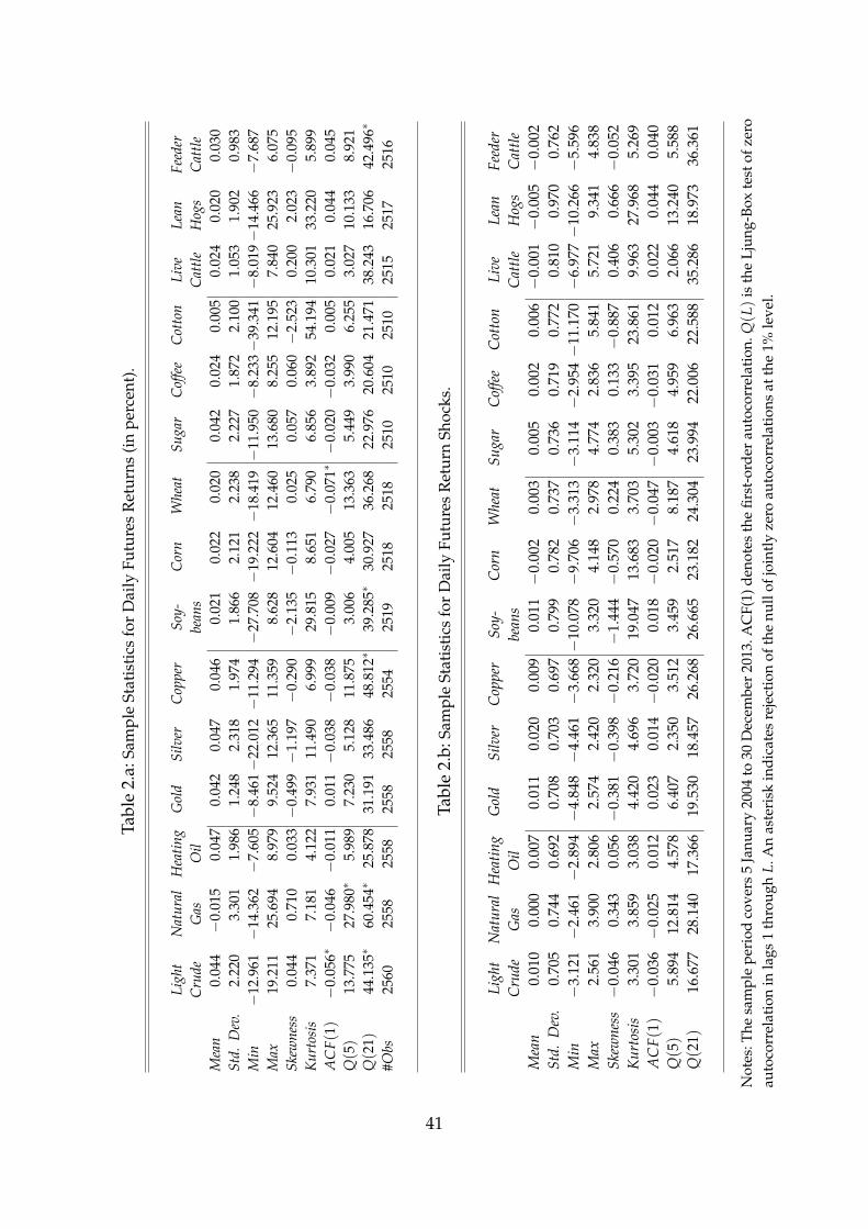
Tabl

e2.

a:Sa

mpl

eSt

atis

tics

for

Dai

lyFu

ture

sR

etur

ns(i

npe

rcen

t).

Ligh

tN

atur

alH

eatin

gG

old

Silv

erC

oppe

rSo

y-C

orn

Whe

atSu

gar

Cof

fee

Cot

ton

Live

Lean

Feed

erC

rude

Gas

Oil

bean

sC

attle

Hog

sC

attle

Mea

n0.

044

−0.

015

0.04

70.

042

0.04

70.

046

0.02

10.

022

0.02

00.

042

0.02

40.

005

0.02

40.

020

0.03

0St

d.D

ev.

2.22

03.

301

1.98

61.

248

2.31

81.

974

1.86

62.

121

2.23

82.

227

1.87

22.

100

1.05

31.

902

0.98

3M

in−

12.9

61−

14.3

62−

7.60

5−

8.46

1−

22.0

12−

11.2

94−

27.7

08−

19.2

22−

18.4

19−

11.9

50−

8.23

3−

39.3

41−

8.01

9−

14.4

66−

7.68

7M

ax19

.211

25.6

948.

979

9.52

412

.365

11.3

598.

628

12.6

0412

.460

13.6

808.

255

12.1

957.

840

25.9

236.

075

Skew

ness

0.04

40.

710

0.03

3−

0.49

9−

1.19

7−

0.29

0−

2.13

5−

0.11

30.

025

0.05

70.

060

−2.

523

0.20

02.

023

−0.

095

Kur

tosi

s7.

371

7.18

14.

122

7.93

111

.490

6.99

929

.815

8.65

16.

790

6.85

63.

892

54.1

9410

.301

33.2

205.

899

AC

F(1)

−0.

056∗

−0.

046

−0.

011

0.01

1−

0.03

8−

0.03

8−

0.00

9−

0.02

7−

0.07

1∗−

0.02

0−

0.03

20.

005

0.02

10.

044

0.04

5Q(5)

13.7

7527

.980

∗5.

989

7.23

05.

128

11.8

753.

006

4.00

513

.363

5.44

93.

990

6.25

53.

027

10.1

338.

921

Q(2

1)44

.135

∗60

.454

∗25

.878

31.1

9133

.486

48.8

12∗

39.2

85∗

30.9

2736

.268

22.9

7620

.604

21.4

7138

.243

16.7

0642

.496

∗

#Obs

2560

2558

2558

2558

2558

2554

2519

2518

2518

2510

2510

2510

2515

2517

2516

Tabl

e2.

b:Sa

mpl

eSt

atis

tics

for

Dai

lyFu

ture

sR

etur

nSh

ocks

.

Ligh

tN

atur

alH

eatin

gG

old

Silv

erC

oppe

rSo

y-C

orn

Whe

atSu

gar

Cof

fee

Cot

ton

Live

Lean

Feed

erC

rude

Gas

Oil

bean

sC

attle

Hog

sC

attle

Mea

n0.

010

0.00

00.

007

0.01

10.

020

0.00

90.

011

−0.

002

0.00

30.

005

0.00

20.

006

−0.

001

−0.

005

−0.

002

Std.

Dev

.0.

705

0.74

40.

692

0.70

80.

703

0.69

70.

799

0.78

20.

737

0.73

60.

719

0.77

20.

810

0.97

00.

762

Min

−3.

121

−2.

461

−2.

894

−4.

848

−4.

461

−3.

668−

10.0

78−

9.70

6−

3.31

3−

3.11

4−

2.95

4−

11.1

70−

6.97

7−

10.2

66−

5.59

6M

ax2.

561

3.90

02.

806

2.57

42.

420

2.32

03.

320

4.14

82.

978

4.77

42.

836

5.84

15.

721

9.34

14.

838

Skew

ness

−0.

046

0.34

30.

056

−0.

381

−0.

398

−0.

216

−1.

444

−0.

570

0.22

40.

383

0.13

3−

0.88

70.

406

0.66

6−

0.05

2K

urto

sis

3.30

13.

859

3.03

84.

420

4.69

63.

720

19.0

4713

.683

3.70

35.

302

3.39

523

.861

9.96

327

.968

5.26

9A

CF(

1)−

0.03

6−

0.02

50.

012

0.02

30.

014

−0.

020

0.01

8−

0.02

0−

0.04

7−

0.00

3−

0.03

10.

012

0.02

20.

044

0.04

0Q(5)

5.89

412

.814

4.57

86.

407

2.35

03.

512

3.45

92.

517

8.18

74.

618

4.95

96.

963

2.06

613

.240

5.58

8Q(2

1)16

.677

28.1

4017

.366

19.5

3018

.457

26.2

6826

.665

23.1

8224

.304

23.9

9422

.006

22.5

8835

.286

18.9

7336

.361

Not

es:T

hesa

mpl

epe

riod

cove

rs5

Janu

ary

2004

to30

Dec

embe

r20

13.A

CF(

1)de

note

sth

efir

st-o

rder

auto

corr

elat

ion.

Q(L)

isth

eLj

ung-

Box

test

ofze

roau

toco

rrel

atio

nin

lags

1th

roug

hL.

An

aste

risk

indi

cate

sre

ject

ion

ofth

enu

llof

join

tly

zero

auto

corr

elat

ions

atth

e1%

leve

l.

41

Tabl

e3.

a:Sa

mpl

eSt

atis

tics

for

Dai

lyR

ealiz

edVo

lati

lity.

Ligh

tN

atur

alH

eatin

gG

old

Silv

erC

oppe

rSo

y-C

orn

Whe

atSu

gar

Cof

fee

Cot

ton

Live

Lean

Feed

erC

rude

Gas

Oil

bean

sC

attle

Hog

sC

attle

Mea

n2.

717

3.95

52.

544

1.52

22.

792

2.38

52.

065

2.48

12.

718

2.68

52.

484

2.40

91.

227

1.88

21.

229

Std.

Dev

.1.

308

1.50

21.

112

0.72

81.

343

1.16

40.

966

1.10

11.

214

1.12

10.

716

1.11

60.

425

0.68

20.

452

Min

0.60

20.

968

0.61

50.

321

0.40

00.

532

0.67

50.

535

0.66

40.

827

1.04

00.

531

0.33

50.

472

0.34

4M

ax11

.026

13.7

0413

.261

8.61

616

.707

11.5

0514

.757

11.7

0828

.304

9.48

36.

997

17.3

413.

925

8.68

44.

478

Skew

ness

2.36

21.

335

1.70

62.

430

2.71

42.

426

2.77

02.

325

5.48

91.

148

1.09

82.

622

1.55

02.

269

1.69

1K

urto

sis

10.5

506.

016

8.95

013

.831

16.0

2712

.420

20.7

1112

.782

88.2

825.

332

5.46

922

.013

7.33

513

.535

8.35

2A

CF(

1)0.

822∗

0.70

1∗0.

779∗

0.76

0∗0.

745∗

0.85

0∗0.

555∗

0.51

8∗0.

547∗

0.75

8∗0.

509∗

0.57

6∗0.

559∗

0.52

7∗0.

584∗

Q(5)

7741

∗52

27∗

6969

∗54

63∗

4951

∗79

54∗

2731

∗18

89∗

2278

∗55

24∗

1858

∗35

62∗

3017

∗25

48∗

3033

∗

Q(2

1)28

206∗

1562

2∗25

122∗

1787

5∗13

619∗

2587

5∗86

98∗

4908

∗63

14∗

1778

7∗42

63∗

1198

6∗10

612∗

8152

∗95

27∗

Tabl

e3.

b:Sa

mpl

eSt

atis

tics

for

Log

Dai

lyR

ealiz

edVo

lati

lity.

Ligh

tN

atur

alH

eatin

gG

old

Silv

erC

oppe

rSo

y-C

orn

Whe

atSu

gar

Cof

fee

Cot

ton

Live

Lean

Feed

erC

rude

Gas

Oil

bean

sC

attle

Hog

sC

attle

Mea

n0.

913

1.31

00.

851

0.33

10.

942

0.77

90.

643

0.83

20.

931

0.90

50.

871

0.79

20.

152

0.57

90.

148

Std.

Dev

.0.

400

0.35

60.

403

0.40

80.

395

0.41

00.

387

0.37

80.

357

0.40

70.

277

0.40

80.

321

0.31

70.

335

Min

−0.

508

−0.

032

−0.

486

−1.

136

−0.

917

−0.

630

−0.

393

−0.

626

−0.

409

−0.

189

0.03

9−

0.63

4−

1.09

5−

0.75

1−

1.06

7M

ax2.

400

2.61

82.

585

2.15

42.

816

2.44

32.

692

2.46

03.

343

2.25

01.

945

2.85

31.

367

2.16

11.

499

Skew

ness

0.54

10.

200

0.15

90.

413

0.59

40.

481

0.66

80.

545

0.51

2−

0.00

10.

109

0.29

50.

202

0.50

60.

305

Kur

tosi

s4.

188

2.90

23.

134

3.73

64.

195

3.80

43.

554

3.63

54.

580

2.60

33.

140

3.24

83.

659

4.04

03.

401

AC

F(1)

0.79

3∗0.

714∗

0.80

1∗0.

735∗

0.72

9∗0.

849∗

0.63

5∗0.

603∗

0.64

6∗0.

792∗

0.53

6∗0.

658∗

0.58

9∗0.

584∗

0.58

8∗

Q(5)

6905

∗55

80∗

7241

∗52

94∗

4924

∗78

67∗

3767

∗30

22∗

3885

∗65

16∗

2274

∗43

86∗

3570

∗31

62∗

3167

∗

Q(2

1)23

915∗

1791

0∗26

090∗

1718

2∗14

035∗

2618

2∗11

942∗

8337

∗11

581∗

2248

1∗54

07∗

1488

7∗12

413∗

1030

3∗10

219∗

Not

es:T

hesa

mpl

epe

riod

cove

rs5

Janu

ary

2004

to30

Dec

embe

r20

13.A

CF(

1)de

note

sth

efir

st-o

rder

auto

corr

elat

ion.

Q(L)

isth

eLj

ung-

Box

test

ofze

roau

toco

rrel

atio

nin

lags

1th

roug

hL.

An

aste

risk

indi

cate

sre

ject

ion

atth

e1%

leve

l.

42

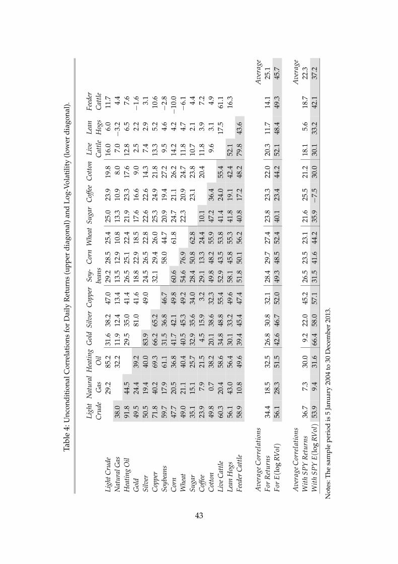
Tabl

e4:

Unc

ondi

tion

alC

orre

lati

ons

for

Dai

lyR

etur

ns(u

pper

diag

onal

)and

Log-

Vola

tilit

y(l

ower

diag

onal

).

Ligh

tN

atur

alH

eatin

gG

old

Silv

erC

oppe

rSo

y-C

orn

Whe

atSu

gar

Cof

fee

Cot

ton

Live

Lean

Feed

erC

rude

Gas

Oil

bean

sC

attle

Hog

sC

attle

Ligh

tCru

de29

.285

.231

.638

.247

.029

.228

.525

.425

.023

.919

.816

.06.

011

.7N

atur

alG

as38

.032

.211

.912

.413

.413

.512

.910

.813

.310

.98.

07.

0−

3.2

4.4

Hea

ting

Oil

91.8

44.5

29.5

35.0

41.4

26.5

25.1

22.4

21.9

23.3

17.6

12.8

6.5

7.6

Gol

d49

.524

.439

.281

.041

.618

.822

.918

.517

.616

.69.

02.

52.

2−

1.6

Silv

er50

.519

.440

.083

.949

.024

.526

.522

.822

.622

.614

.37.

42.

93.

1C

oppe

r71

.840

.269

.366

.265

.232

.129

.426

.025

.324

.921

.813

.35.

210

.6So

ybea

ns59

.717

.961

.131

.536

.846

.758

.044

.720

.919

.427

.29.

54.

6−

2.8

Cor

n47

.720

.536

.841

.742

.149

.860

.661

.824

.721

.126

.214

.24.

2−

10.0

Whe

at49

.021

.140

.440

.545

.349

.254

.676

.922

.320

.924

.711

.84.

7−

6.1

Suga

r35

.115

.125

.732

.935

.634

.028

.450

.862

.823

.123

.810

.72.

14.

4C

offe

e23

.97.

921

.54.

515

.93.

229

.113

.324

.410

.120

.411

.83.

97.

2C

otto

n49

.80.

738

.220

.138

.632

.349

.848

.255

.947

.236

.49.

63.

14.

9Li

veC

attle

60.3

20.4

58.6

34.8

48.8

55.4

52.9

43.5

53.8

41.4

24.0

55.4

17.5

61.1

Lean

Hog

s56

.143

.056

.430

.133

.249

.658

.145

.855

.341

.819

.142

.452

.116

.3Fe

eder

Cat

tle58

.910

.849

.639

.445

.447

.451

.850

.156

.240

.817

.248

.279

.843

.6

Ave

rage

Cor

rela

tion

sA

vera

geFo

rR

etur

ns34

.418

.532

.526

.830

.832

.128

.429

.727

.423

.823

.322

.020

.311

.714

.125

.1Fo

rE(l

ogRV

ol)

56.1

28.3

51.5

42.6

46.7

52.0

49.3

48.5

52.4

40.1

23.4

44.2

52.1

48.4

49.3

45.7

Ave

rage

Cor

rela

tion

sA

vera

geW

ith

SPY

Ret

urns

36.7

7.3

30.0

9.2

22.0

45.2

26.5

23.5

23.1

21.6

25.5

21.2

18.1

5.6

18.7

22.3

Wit

hSP

YE(l

ogRV

ol)

53.9

9.4

31.6

66.4

58.0

57.1

31.5

41.6

44.2

35.9

−7.

530

.030

.133

.242

.137

.2

Not

es:T

hesa

mpl

epe

riod

is5

Janu

ary

2004

to30

Dec

embe

r20

13.

43

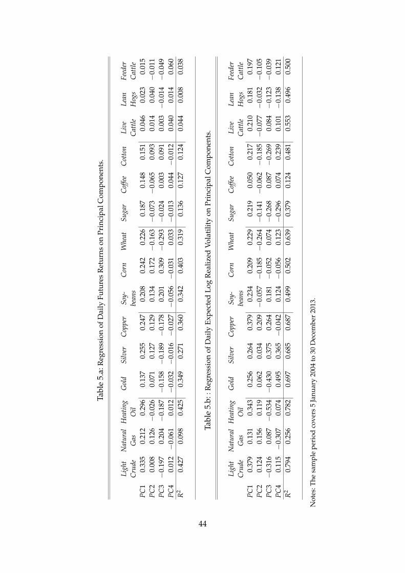
Tabl

e5.

a:R

egre

ssio

nof

Dai

lyFu

ture

sR

etur

nson

Prin

cipa

lCom

pone

nts.

Ligh

tN

atur

alH

eatin

gG

old

Silv

erC

oppe

rSo

y-C

orn

Whe

atSu

gar

Cof

fee

Cot

ton

Live

Lean

Feed

erC

rude

Gas

Oil

bean

sC

attle

Hog

sC

attle

PC

10.

335

0.21

20.

296

0.13

70.

255

0.24

70.

208

0.24

20.

226

0.18

70.

148

0.15

10.

046

0.02

30.

015

PC

20.

008

0.12

6−

0.02

60.

071

0.12

70.

129

0.13

40.

172

−0.

163

−0.

073

−0.

065

0.09

30.

014

0.04

0−

0.01

1P

C3

−0.

197

0.20

4−

0.18

7−

0.15

8−

0.18

9−

0.17

80.

201

0.30

9−

0.29

3−

0.02

40.

003

0.09

10.

003

−0.

014

−0.

049

PC

40.

012

−0.

061

0.01

2−

0.03

2−

0.01

6−

0.02

7−

0.05

6−

0.03

10.

033

−0.

013

0.04

4−

0.01

20.

040

0.01

40.

060

R2

0.42

70.

098

0.42

50.

349

0.27

10.

360

0.34

20.

403

0.31

90.

136

0.12

70.

124

0.04

40.

008

0.03

8

Tabl

e5.

b::R

egre

ssio

nof

Dai

lyEx

pect

edLo

gR

ealiz

edVo

lati

lity

onPr

inci

palC

ompo

nent

s.

Ligh

tN

atur

alH

eatin

gG

old

Silv

erC

oppe

rSo

y-C

orn

Whe

atSu

gar

Cof

fee

Cot

ton

Live

Lean

Feed

erC

rude

Gas

Oil

bean

sC

attle

Hog

sC

attle

PC

10.

379

0.13

10.

343

0.25

60.

264

0.37

90.

234

0.20

90.

229

0.21

90.

050

0.21

70.

210

0.18

10.

197

PC

20.

124

0.15

60.

119

0.06

20.

034

0.20

9−

0.05

7−

0.18

5−

0.26

4−

0.14

1−

0.06

2−

0.18

5−

0.07

7−

0.03

2−

0.10

5P

C3

−0.

316

0.08

7−

0.53

4−

0.43

00.

375

0.26

40.

181

−0.

052

0.07

4−

0.26

80.

087

−0.

269

0.08

4−

0.12

3−

0.03

9P

C4

0.11

5−

0.30

70.

074

0.49

50.

365

−0.

042

0.12

4−

0.05

60.

123

−0.

296

0.07

40.

239

0.10

1−

0.13

80.

121

R2

0.79

40.

256

0.78

20.

697

0.68

50.

687

0.49

90.

502

0.63

90.

379

0.12

40.

481

0.55

30.

496

0.50

0

Not

es:T

hesa

mpl

epe

riod

cove

rs5

Janu

ary

2004

to30

Dec

embe

r20

13.

44

Reg

ress

ion

ofD

aily

Futu

res

Ret

urns

onSp

yder

and

Spyd

er-O

rtho

gona

lPri

ncip

alC

ompo

nent

s.

Tabl

e6.

a:R

esul

tsfo

rR

etur

ns:r

Com

,t=

α+

βSP

Yr S

PY,t+

βˆ

PC

1ˆ

PC

1+

βˆ

PC

2ˆ

PC

2+

βˆ

PC

3ˆ

PC

3+

βˆ

PC

4ˆ

PC

4+

ε t

Ligh

tN

atur

alH

eatin

gG

old

Silv

erC

oppe

rSo

y-C

orn

Whe

atSu

gar

Cof

fee

Cot

ton

Live

Lean

Feed

erC

rude

Gas

Oil

bean

sC

attle

Hog

sC

attle

Con

stan

t0.

028

−0.

024

0.03

50.

038

0.03

40.

026

0.01

30.

009

0.00

90.

028

0.01

0−

0.00

40.

018

0.01

30.

025

r SPY

0.65

6∗0.

203∗

0.50

2∗0.

147∗

0.54

5∗0.

702∗

0.40

4∗0.

409∗

0.42

4∗0.

389∗

0.41

8∗0.

365∗

0.14

8∗0.

140∗

0.14

9∗ˆ

PC

10.

312∗

0.21

7∗0.

299∗

0.13

5∗0.

207∗

0.19

4∗0.

178∗

0.19

9∗0.

188∗

0.15

7∗0.

118∗

0.12

6∗0.

039∗

0.04

0∗0.

005

ˆP

C2

0.02

3−

0.14

9∗−

0.01

50.

117∗

−0.

167∗

−0.

120∗

0.15

8∗−

0.18

5∗0.

190∗

0.09

4∗0.

071∗

0.11

2∗0.

016

−0.

026

−0.

021∗

ˆP

C3

−0.

176∗

−0.

240∗

−0.

167∗

−0.

167∗

0.16

6∗0.

189∗

0.20

1∗−

0.29

4∗0.

294∗

0.03

40.

017

0.06

2∗−

0.00

3−

0.01

1−

0.04

4∗ˆ

PC

40.

063∗

−0.

078

0.06

5∗−

0.09

8∗0.

034

−0.

030

0.04

5∗−

0.11

3∗−

0.08

2∗0.

033

0.02

40.

052∗

0.01

60.

003

0.02

9∗

R2

0.44

00.

108

0.42

00.

375

0.26

50.

379

0.34

90.

373

0.32

80.

137

0.14

00.

129

0.05

20.

015

0.05

8

Tabl

e6.

b:R

esul

tsfo

rVo

lati

lity:

E(l

ogRV

olC

om,t)=

α+

βSP

YE(l

ogRV

olSP

Y,t)+

βˆ

PC

1ˆ

PC

1+

βˆ

PC

2ˆ

PC

2+

βˆ

PC

3ˆ

PC

3+

βˆ

PC

4ˆ

PC

4+

ε t

Ligh

tN

atur

alH

eatin

gG

old

Silv

erC

oppe

rSo

y-C

orn

Whe

atSu

gar

Cof

fee

Cot

ton

Live

Lean

Feed

erC

rude

Gas

Oil

bean

sC

attle

Hog

sC

attle

Con

stan

t0.

691∗

0.95

6∗0.

588∗

0.10

2∗0.

666∗

0.58

3∗0.

375∗

0.55

6∗0.

651∗

0.60

1∗0.

522∗

0.55

3∗−

0.12

5∗0.

322∗

−0.

107∗

E(l

ogRV

olSP

Y)

0.46

4∗0.

044

0.31

0∗0.

470∗

0.38

9∗0.

477∗

0.22

7∗0.

241∗

0.27

3∗0.

219∗

0.01

40.

206∗

0.17

6∗0.

165∗

0.22

6∗ˆ

PC

10.

368∗

0.23

2∗0.

443∗

0.12

2∗0.

168∗

0.32

9∗0.

257∗

0.14

4∗0.

182∗

0.19

2∗0.

075∗

0.20

6∗0.

245∗

0.20

7∗0.

192∗

ˆP

C2

0.20

2∗−

0.01

60.

132∗

0.09

6∗−

0.11

7∗0.

084∗

−0.

094

0.11

0∗−

0.10

9∗0.

094

−0.

114∗

−0.

034

0.00

50.

079∗

0.02

7ˆ

PC

3−

0.24

9∗−

0.22

2∗−

0.51

5∗0.

470∗

0.34

7∗−

0.31

9∗0.

182∗

0.16

5∗0.

274∗

0.28

3∗0.

104∗

0.32

7∗0.

129∗

0.02

50.

147∗

ˆP

C4

0.03

80.

123

0.00

70.

390∗

−0.

180∗

0.09

80.

100

0.01

90.

045

−0.

116

−0.

006

0.06

40.

125∗

−0.

106

0.14

5∗

R2

0.83

10.

334

0.82

40.

736

0.64

40.

717

0.52

00.

448

0.60

70.

330

0.16

30.

474

0.59

00.

508

0.53

2

Not

es:C

omm

odit

yre

turn

san

dex

pect

edlo

gvo

lati

lity

are

regr

esse

don

Spyd

erre

turn

san

dex

pect

edlo

gvo

lati

lity.

Toav

oid

end

ogen

eity

the

prin

cipa

lco

mp

onen

tsar

eba

sed

onth

eu

ncon

dit

iona

lco

vari

ance

mat

rix

ofth

ed

emea

ned

regr

essi

onre

sid

ual

sfo

rth

e14

othe

rco

mm

odit

ies.

The

pri

ncip

alco

mpo

nent

sar

eco

nstr

ucte

das

the

mat

rix

ofre

sid

uals

mul

tipl

ied

byth

eei

genv

ecto

rsof

the

cova

rian

cem

atri

x.Si

gnifi

canc

eat

the

1%le

velw

hen

usin

gH

AC

stan

dard

erro

rsis

indi

cate

dby

anas

teri

sk.

45

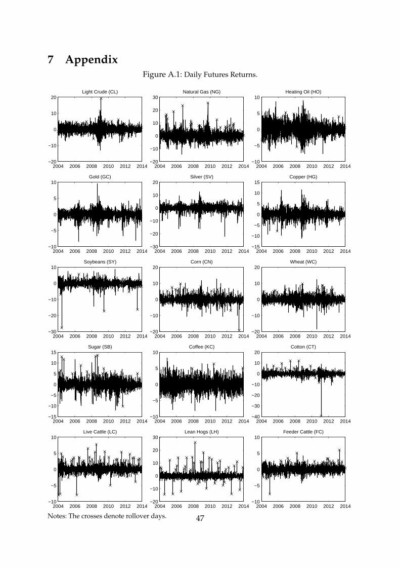
7 AppendixFigure A.1: Daily Futures Returns.

2004 2006 2008 2010 2012 2014−20

−10

0

10

20Light Crude (CL)

2004 2006 2008 2010 2012 2014−20

−10

0

10

20

30Natural Gas (NG)

2004 2006 2008 2010 2012 2014−10

−5

0

5

10Heating Oil (HO)

2004 2006 2008 2010 2012 2014−10

−5

0

5

10Gold (GC)

2004 2006 2008 2010 2012 2014−30

−20

−10

0

10

20Silver (SV)

2004 2006 2008 2010 2012 2014−15

−10

−5

0

5

10

15Copper (HG)

2004 2006 2008 2010 2012 2014−30

−20

−10

0

10Soybeans (SY)

2004 2006 2008 2010 2012 2014−20

−10

0

10

20Corn (CN)

2004 2006 2008 2010 2012 2014−20

−10

0

10

20Wheat (WC)

2004 2006 2008 2010 2012 2014−15

−10

−5

0

5

10

15Sugar (SB)

2004 2006 2008 2010 2012 2014−10

−5

0

5

10Coffee (KC)

2004 2006 2008 2010 2012 2014−40

−30

−20

−10

0

10

20Cotton (CT)

2004 2006 2008 2010 2012 2014−10

−5

0

5

10Live Cattle (LC)

2004 2006 2008 2010 2012 2014−20

−10

0

10

20

30Lean Hogs (LH)

2004 2006 2008 2010 2012 2014−10

−5

0

5

10Feeder Cattle (FC)

Notes: The crosses denote rollover days. 47

Figure A.2: Autocorrelation Function of Daily Futures Returns.

10 20 30 40 50 60−0.1

−0.05

0

0.05

0.1Light Crude (CL)

10 20 30 40 50 60−0.1

−0.05

0

0.05

0.1Natural Gas (NG)

10 20 30 40 50 60−0.1

−0.05

0

0.05

0.1Heating Oil (HO)

10 20 30 40 50 60−0.1

−0.05

0

0.05

0.1Gold (GC)

10 20 30 40 50 60−0.1

−0.05

0

0.05

0.1Silver (SV)

10 20 30 40 50 60−0.1

−0.05

0

0.05

0.1Copper (HG)

10 20 30 40 50 60−0.1

−0.05

0

0.05

0.1Soybeans (SY)

10 20 30 40 50 60−0.1

−0.05

0

0.05

0.1Corn (CN)

10 20 30 40 50 60−0.1

−0.05

0

0.05

0.1Wheat (WC)

10 20 30 40 50 60−0.1

−0.05

0

0.05

0.1Sugar (SB)

10 20 30 40 50 60−0.1

−0.05

0

0.05

0.1Coffee (KC)

10 20 30 40 50 60−0.1

−0.05

0

0.05

0.1Cotton (CT)

10 20 30 40 50 60−0.1

−0.05

0

0.05

0.1Live Cattle (LC)

10 20 30 40 50 60−0.1

−0.05

0

0.05

0.1Lean Hogs (LH)

10 20 30 40 50 60−0.1

−0.05

0

0.05


Notes: Grey lines indicate 99% confidence bounds assuming that the series are Gaussian white noise. Thehorizontal axis indicates the lag order in days.

48

Figure A.3: Daily Realized Volatility.

2004 2006 2008 2010 2012 20140

5

10

15Light Crude (CL)

2004 2006 2008 2010 2012 20140

5

10

15Natural Gas (NG)

2004 2006 2008 2010 2012 20140

5

10

15Heating Oil (HO)

2004 2006 2008 2010 2012 20140

2

4

6

8

10Gold (GC)

2004 2006 2008 2010 2012 20140

5

10

15

20Silver (SV)

2004 2006 2008 2010 2012 20140

5

10

15Copper (HG)

2004 2006 2008 2010 2012 20140

5

10

15Soybeans (SY)

2004 2006 2008 2010 2012 20140

5

10

15Corn (CN)

2004 2006 2008 2010 2012 20140

10

20

30Wheat (WC)

2004 2006 2008 2010 2012 20140

2

4

6

8

10Sugar (SB)

2004 2006 2008 2010 2012 20140

2

4

6

8Coffee (KC)

2004 2006 2008 2010 2012 20140

5

10

15

20Cotton (CT)

2004 2006 2008 2010 2012 20140

1

2

3

4Live Cattle (LC)

2004 2006 2008 2010 2012 20140

2

4

6

8

10Lean Hogs (LH)

2004 2006 2008 2010 2012 20140

1

2

3

4

5Feeder Cattle (FC)

Notes: The crosses denote rollover days.

49

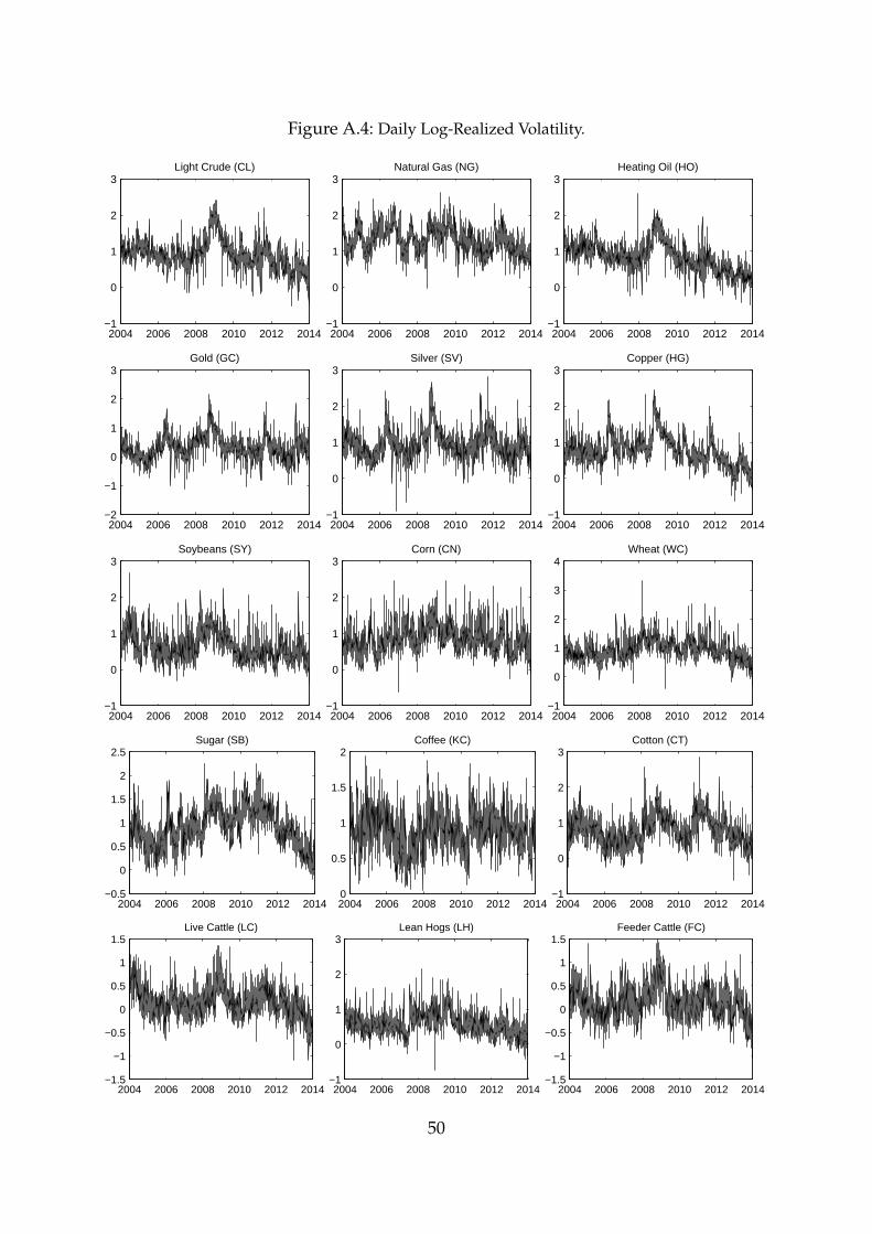
Figure A.4: Daily Log-Realized Volatility.

2004 2006 2008 2010 2012 2014−1

0

1

2

3Light Crude (CL)

2004 2006 2008 2010 2012 2014−1

0

1

2

3Natural Gas (NG)

2004 2006 2008 2010 2012 2014−1

0

1

2

3Heating Oil (HO)

2004 2006 2008 2010 2012 2014−2

−1

0

1

2

3Gold (GC)

2004 2006 2008 2010 2012 2014−1

0

1

2

3Silver (SV)

2004 2006 2008 2010 2012 2014−1

0

1

2

3Copper (HG)

2004 2006 2008 2010 2012 2014−1

0

1

2

3Soybeans (SY)

2004 2006 2008 2010 2012 2014−1

0

1

2

3Corn (CN)

2004 2006 2008 2010 2012 2014−1

0

1

2

3

4Wheat (WC)

2004 2006 2008 2010 2012 2014−0.5

0

0.5

1

1.5

2

2.5Sugar (SB)

2004 2006 2008 2010 2012 20140

0.5

1

1.5

2Coffee (KC)

2004 2006 2008 2010 2012 2014−1

0

1

2

3Cotton (CT)

2004 2006 2008 2010 2012 2014−1.5

−1

−0.5

0

0.5

1

1.5Live Cattle (LC)

2004 2006 2008 2010 2012 2014−1

0

1

2

3Lean Hogs (LH)

2004 2006 2008 2010 2012 2014−1.5

−1

−0.5

0

0.5

1


50

Figure A.5: Realized Stock Market Beta for 15 Commodities.

2004 2006 2008 2010 2012 2014−6

−4

−2

0

2

4Light Crude (CL)

2004 2006 2008 2010 2012 2014−6

−4

−2

0

2

4Natural Gas (NG)

2004 2006 2008 2010 2012 2014−6

−4

−2

0

2Heating Oil (HO)

2004 2006 2008 2010 2012 2014−2

−1

0

1

2

3Gold (GC)

2004 2006 2008 2010 2012 2014−2

0

2

4

6Silver (SV)

2004 2006 2008 2010 2012 2014−2

−1

0

1

2Copper (HG)

2004 2006 2008 2010 2012 2014−4

−2

0

2

4

6Soybeans (SY)

2004 2006 2008 2010 2012 2014−3

−2

−1

0

1

2

3Corn (CN)

2004 2006 2008 2010 2012 2014−4

−2

0

2

4Wheat (WC)

2004 2006 2008 2010 2012 2014−4

−2

0

2

4

6Sugar (SB)

2004 2006 2008 2010 2012 2014−4

−2

0

2

4Coffee (KC)

2004 2006 2008 2010 2012 2014−3

−2

−1

0

1

2

3Cotton (CT)

2004 2006 2008 2010 2012 2014−1.5

−1

−0.5

0

0.5

1

1.5Live Cattle (LC)

2004 2006 2008 2010 2012 2014−2

−1

0

1

2

3Lean Hogs (LH)

2004 2006 2008 2010 2012 2014−2

−1

0

1

2Feeder Cattle (FC)

51

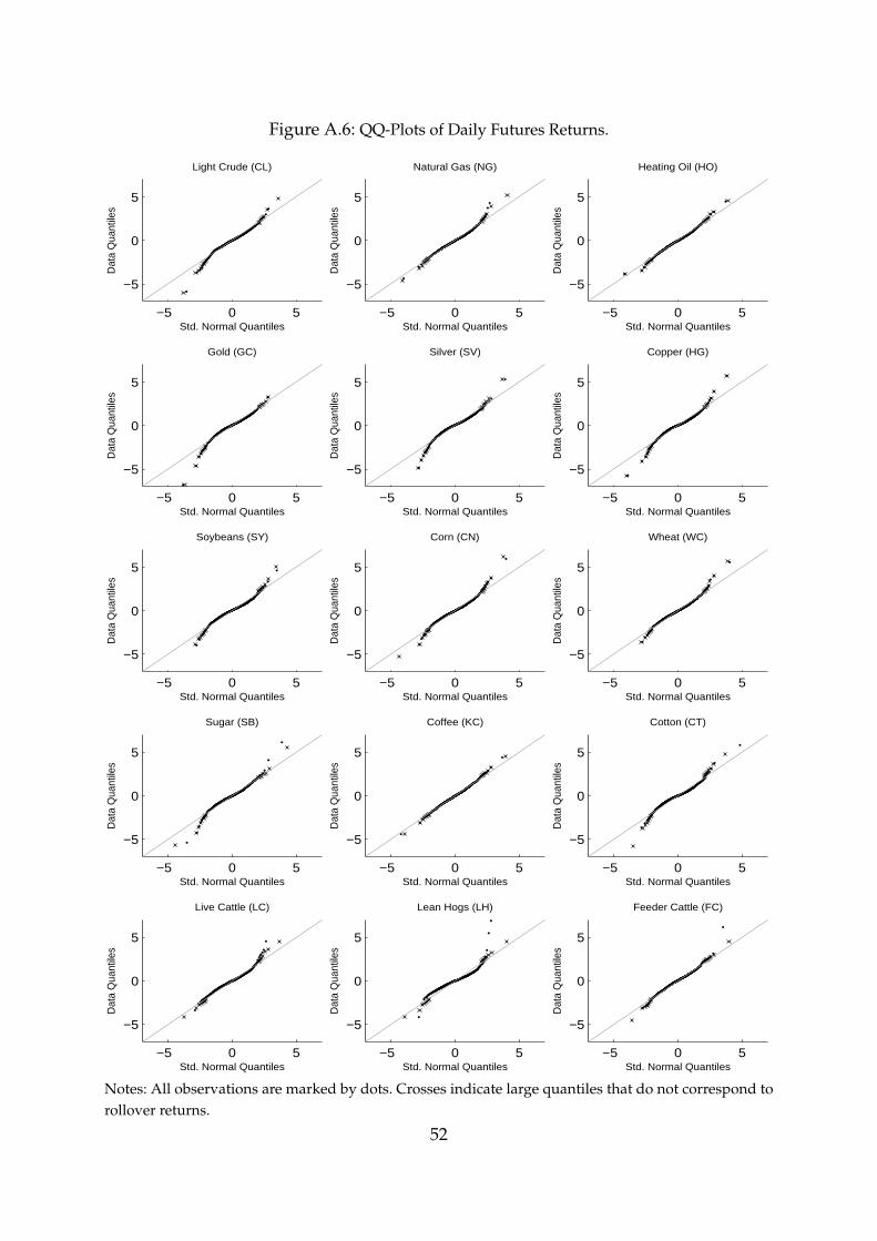
Figure A.6: QQ-Plots of Daily Futures Returns.

−5 0 5

−5

0

5


Dat

a Q

uant

iles

Light Crude (CL)

−5 0 5

−5

0

5


ata

Qua

ntile

s

Natural Gas (NG)

−5 0 5

−5

0

5


Dat

a Q

uant

iles

Heating Oil (HO)

−5 0 5

−5

0

5


Dat

a Q

uant

iles

Gold (GC)

−5 0 5

−5

0

5


Dat

a Q

uant

iles

Silver (SV)

−5 0 5

−5

0

5


Dat

a Q

uant

iles

Copper (HG)

−5 0 5

−5

0

5


Dat

a Q

uant

iles

Soybeans (SY)

−5 0 5

−5

0

5


Dat

a Q

uant

iles

Corn (CN)

−5 0 5

−5

0

5


Dat

a Q

uant

iles

Wheat (WC)

−5 0 5

−5

0

5


Dat

a Q

uant

iles

Sugar (SB)

−5 0 5

−5

0

5


Dat

a Q

uant

iles

Coffee (KC)

−5 0 5

−5

0

5


Dat

a Q

uant

iles

Cotton (CT)

−5 0 5

−5

0

5


Dat

a Q

uant

iles

Live Cattle (LC)

−5 0 5

−5

0

5


Dat

a Q

uant

iles

Lean Hogs (LH)

−5 0 5

−5

0

5


Dat

a Q

uant

iles

Feeder Cattle (FC)


52

Figure A.7: Threshold Correlation Between Daily Commodity Return Shocks and Spyder.

0.2 0.4 0.6 0.8

−0.2

0

0.2

0.4

0.6

Light Crude (CL)

0.2 0.4 0.6 0.8

−0.2

0

0.2

0.4

0.6

Natural Gas (NG)

0.2 0.4 0.6 0.8

−0.2

0

0.2

0.4

0.6

Heating Oil (HO)

0.2 0.4 0.6 0.8

−0.2

0

0.2

0.4

0.6

Gold (GC)

0.2 0.4 0.6 0.8

−0.2

0

0.2

0.4

0.6

Silver (SV)

0.2 0.4 0.6 0.8

−0.2

0

0.2

0.4

0.6

Copper (HG)

0.2 0.4 0.6 0.8

−0.2

0

0.2

0.4

0.6

Soybeans (SY)

0.2 0.4 0.6 0.8

−0.2

0

0.2

0.4

0.6

Corn (CN)

0.2 0.4 0.6 0.8

−0.2

0

0.2

0.4

0.6

Wheat (WC)

0.2 0.4 0.6 0.8

−0.2

0

0.2

0.4

0.6

Sugar (SB)

0.2 0.4 0.6 0.8

−0.2

0

0.2

0.4

0.6

Coffee (KC)

0.2 0.4 0.6 0.8

−0.2

0

0.2

0.4

0.6

Cotton (CT)

0.2 0.4 0.6 0.8

−0.2

0

0.2

0.4

0.6

Live Cattle (LC)

0.2 0.4 0.6 0.8

−0.2

0

0.2

0.4

0.6

Lean Hogs (LH)

0.2 0.4 0.6 0.8

−0.2

0

0.2

0.4

0.6

Feeder Cattle (FC)

Notes: Threshold correlations with rollover days included (black lines) and with rollover days excluded(grey lines). The dashed lines denote threshold correlations for the bivariate Gaussian distribution. Thehorizontal axis indicates thresholds in percentiles.

53

Tabl

eA

.1.a

:Sam

ple

Stat

isti

csfo

rD

aily

Futu

res

Ret

urns

(in

perc

ent)

.Rol

love

rD

ays

Excl

uded

.

Ligh

tN

atur

alH

eatin

gG

old

Silv

erC

oppe

rSo

y-C

orn

Whe

atSu

gar

Cof

fee

Cot

ton

Live

Lean

Feed

erC

rude

Gas

Oil

bean

sC

attle

Hog

sC

attle

Mea

n−

0.00

8−

0.16

70.

031

0.03

70.

046

0.04

60.

042

−0.

012

−0.

042

0.00

3−

0.00

9−

0.00

9−

0.00

5−

0.03

80.

014

Std.

Dev

.2.

163

3.10

81.

979

1.25

32.

328

1.96

51.

700

2.03

32.

192

2.11

21.

852

1.86

50.

915

1.35

20.

929

Min

−12

.961

−14

.362

−7.

605

−8.

461−

22.0

12−

11.2

94−

14.3

37−

10.7

31−

18.4

19−

11.9

50−

8.23

3−

10.7

94−

3.79

9−

5.58

2−

4.20

6M

ax10

.552

16.0

598.

979

9.52

412

.365

11.3

598.

628

12.6

0412

.460

11.5

748.

255

8.94

34.

148

5.99

84.

166

Skew

ness

−0.

284

0.19

90.

029

−0.

495

−1.

208

−0.

278

−0.

351

0.09

0−

0.05

8−

0.27

20.

035

−0.

142

0.15

00.

003

−0.

113

Kur

tosi

s5.

404

4.44

94.

192

7.92

911

.495

7.04

57.

187

6.42

96.

994

5.63

43.

941

5.85

64.

400

3.96

93.

840

AC

F(1)

−0.

030

−0.

055∗

−0.

015

0.01

0−

0.03

5−

0.03

5−

0.01

3−

0.02

3−

0.06

0∗−

0.03

5−

0.02

20.

018

0.01

40.

078∗

0.04

5Q(5)

4.02

222

.212

∗5.

737

7.12

15.

038

10.4

483.

320

5.42

610

.917

8.08

93.

768

8.21

24.

518

21.5

25∗

8.94

5Q(2

1)47

.762

∗32

.954

32.8

3323

.821

21.7

2750

.120

∗41

.859

∗24

.598

22.2

3236

.752

27.7

7234

.494

39.2

80∗

53.7

95∗

47.0

43∗

Tabl

eA

.1.b

:Sam

ple

Stat

isti

csfo

rD

aily

Ret

urn

Shoc

ks.R

ollo

ver

Day

sEx

clud

ed.

Ligh

tN

atur

alH

eatin

gG

old

Silv

erC

oppe

rSo

y-C

orn

Whe

atSu

gar

Cof

fee

Cot

ton

Live

Lean

Feed

erC

rude

Gas

Oil

bean

sC

attle

Hog

sC

attle

Mea

n0.

014

0.00

70.

006

0.01

00.

019

0.00

90.

008

−0.

002

0.00

50.

005

0.00

20.

002

−0.

001

0.00

2−

0.00

3St

d.D

ev.

0.69

70.

715

0.68

70.

708

0.70

70.

692

0.73

40.

732

0.72

20.

698

0.71

30.

700

0.69

70.

690

0.72

2M

in−

3.07

6−

2.58

0−

2.85

0−

4.84

0−

4.47

2−

2.87

7−

3.33

4−

4.21

8−

3.32

0−

2.65

9−

2.95

2−

5.16

4−

2.25

2−

2.69

6−

2.85

3M

ax2.

470

2.73

12.

773

2.57

62.

419

2.52

63.

264

2.91

82.

909

4.18

64.

007

3.04

42.

973

3.07

32.

299

Skew

ness

−0.

087

0.10

30.

037

−0.

385

−0.

433

−0.

165

−0.

075

−0.

023

0.13

10.

097

0.13

1−

0.16

70.

072

−0.

002

−0.

161

Kur

tosi

s3.

253

3.04

32.

999

4.42

94.

852

3.52

83.

820

4.15

33.

725

3.95

03.

680

5.05

43.

368

3.32

53.

322

AC

F(1)

−0.

024

−0.

022

0.01

60.

021

0.01

6−

0.01

80.

007

−0.

016

−0.

031

−0.

011

−0.

025

0.02

00.

012

0.08

7∗0.

045

Q(5)

2.94

27.

808

3.40

66.

186

2.69

74.

490

4.23

83.

037

5.14

25.

630

5.82

18.

505

2.17

223

.770

∗7.

338

Q(2

1)17

.901

14.9

8613

.218

15.2

9914

.033

33.5

8229

.865

17.5

1010

.458

32.7

8327

.708

25.5

5133

.346

50.4

15∗

36.2

49

Not

es:T

hesa

mp

lep

erio

dco

vers

5Ja

nuar

y20

04to

30D

ecem

ber

2013

.AC

F(1)

isth

efi

rst-

ord

erau

toco

rrel

atio

n.Q(L)

isth

eL

jung

-Box

test

ofze

roau

to-c

orre

lati

onin

lags

1th

roug

hL.

An

aste

risk

indi

cate

sre

ject

ion

atth

e1

perc

entl

evel

.

54

Tabl

eA

.2:O

ptim

alW

eigh

tson

Ope

n-to

-Clo

seR

ealiz

edVo

lati

lity

and

Ove

rnig

htR

etur

ns.

Ligh

tN

atur

alH

eatin

gG

old

Silv

erC

oppe

rSo

y-C

orn

Whe

atSu

gar

Cof

fee

Cot

ton

Live

Lean

Feed

erC

rude

Gas

Oil

bean

sC

attle

Hog

sC

attle

E[ ( rco i,t

) 2 +RV

i,t

]8.

110

16.9

267.

136

2.53

98.

471

6.29

34.

668

6.71

77.

837

7.98

16.

449

6.42

21.

600

3.71

21.

614

E[ ( rco i,t

) 2]3.

995

8.87

93.

449

1.24

94.

045

3.12

82.

502

3.64

44.

160

3.97

13.

118

3.10

10.

853

1.98

60.

831

E[R

Vi,t]

4.11

58.

047

3.68

71.

289

4.42

63.

164

2.16

53.

073

3.67

74.

010

3.33

13.

321

0.74

71.

726

0.78

2

E[R

Vi,t]

E[ (r

co i,t)2]

1.03

00.

906

1.06

91.

032

1.09

41.

012

0.86

50.

844

0.88

41.

010

1.06

81.

071

0.87

50.

869

0.94

1

E

[ ( (rco i,t

) 2 −E[ ( rco i,t

) 2])2]

43.5

0118

8.27

926

.970

4.45

351

.291

31.8

9519

.028

40.0

9945

.252

43.3

1520

.498

30.9

542.

210

14.4

761.

625

E[ ( RV

i,t−

E[R

Vi,t]) 2]

18.5

6336

.166

10.5

011.

466

17.7

699.

901

4.16

37.

992

8.42

710

.224

3.62

68.

759

0.26

81.

417

0.33

9

E[ (R

Vi,t−

E[R

Vi,t])

2]E[ ( (r

co i,t)2 −

E[ (r

co i,t)2]) 2

]0.

427

0.19

20.

389

0.32

90.

346

0.31

00.

219

0.19

90.

186

0.23

60.

177

0.28

30.

121

0.09

80.

209

E[ RV

i,t

( (rco i,t)2 −

E[ (r

co i,t)2])]

E[ (r

co i,t)2 −

E[ (r

co i,t)2]] ·E

[RV

i,t−

E[R

Vi,t]]

0.43

70.

356

0.40

40.

385

0.40

00.

455

0.26

50.

278

0.30

20.

382

0.19

80.

331

0.23

60.

204

0.23

0

ϕ0.

852

0.93

00.

879

0.89

20.

913

0.93

40.

852

0.86

50.

904

0.94

50.

923

0.91

00.

933

0.94

30.

877

ω? 1

0.30

00.

133

0.25

00.

220

0.18

10.

133

0.27

60.

249

0.18

10.

111

0.15

90.

186

0.12

50.

107

0.23

8

ω? 2

1.68

01.

957

1.70

21.

756

1.74

81.

857

1.83

71.

890

1.92

61.

881

1.78

71.

760

2.00

02.

028

1.80

9

Not

es:T

heta

ble

cont

ains

the

wei

ghti

ngpa

ram

eter

sth

atar

eus

edto

com

pute

the

opti

mal

mea

sure

ofda

ilyvo

lati

lity

ineq

uati

on.

ϕ≡

E[R

Vi,t]2

E

[ ( (rco i,t

) 2 −E[ ( rco i,t

) 2])2] −

E[ ( rco i,t

) 2] E[R

Vi,t]E[ RV

i,t

( ( rco i,t

) 2 −E[ ( rco i,t

) 2])]

E[R

Vi,t]2

E

[ ( (rco i,t

) 2 −E[ ( rco i,t

) 2])2] +

E[ ( rco i,t

) 2] 2E[ ( RV

i,t−

E[R

Vi,t]) 2]

−2E[ ( rco i,t

) 2] E[R

Vi,t]E[ RV

i,t

( ( rco i,t

) 2 −E[ ( rco i,t

) 2])]

ω? 1≡

(1−

ϕ)

E[ ( rco i,t

) 2 +RV

i,t

]E[ ( rco i,t

) 2],

ω? 2≡

ϕ

E[ ( rco i,t

) 2 +RV

i,t

]E[R

Vi,t]

.

Not

eth

at,a

sex

pect

ed,t

heim

port

ance

fact

or,ϕ

,is

clos

eto

one

inal

lcas

es,w

hich

caus

esth

ere

aliz

edva

rian

cefo

rth

e“a

ctiv

e”pe

riod

,RV

i,t,t

obe

scal

ed

upw

ard

(ω2>

1),w

here

asth

esq

uare

dov

erni

ghtr

etur

n,( rco i,t

) 2 ,is

scal

eddo

wnw

ard

(ω1<

1).

55

Tabl

eA

.3.a

:AR

MA

(1,1

)on

Log

Rea

lized

Vola

tilit

y.

Ligh

tN

atur

alH

eatin

gG

old

Silv

erC

oppe

rSo

y-C

orn

Whe

atSu

gar

Cof

fee

Cot

ton

Live

Lean

Feed

erC

rude

Gas

Oil

bean

sC

attle

Hog

sC

attle

φ0

0.01

60.

026

0.01

10.

013

0.06

00.

022

0.01

60.

040

0.02

90.

024

0.05

90.

014

0.00

10.

012

0.00

3φ

10.

982

0.98

00.

986

0.96

10.

936

0.97

20.

975

0.95

20.

968

0.97

40.

933

0.98

20.

987

0.97

90.

980

θ 1−

0.68

4−

0.73

8−

0.71

8−

0.62

9−

0.52

9−

0.54

7−

0.75

5−

0.68

9−

0.71

5−

0.63

7−

0.67

1−

0.78

2−

0.83

9−

0.79

8−

0.80

1R

20.

696

0.60

30.

715

0.59

00.

570

0.75

60.

484

0.41

80.

492

0.68

00.

346

0.53

50.

479

0.44

00.

441

σe

0.22

00.

225

0.21

50.

261

0.25

90.

203

0.27

80.

288

0.25

40.

230

0.22

40.

278

0.23

20.

237

0.25

1A

CF e(1)

0.09

7∗0.

093∗

0.10

1∗0.

119∗

0.08

9∗0.

097∗

0.12

6∗0.

127∗

0.11

6∗0.

110∗

0.09

0∗0.

109∗

0.09

3∗0.

117∗

0.12

4∗

Qe(

5)50

.305

∗82

.743

∗48

.632

∗98

.360

∗83

.465

∗95

.605

∗73

.091

∗90

.471

∗64

.568

∗68

.131

∗49

.283

∗51

.811

∗29

.714

∗53

.743

∗58

.806

∗

Qe(

21)

96.0

87∗

236.

965∗

91.6

53∗

170.

809∗

122.

133∗

132.

838∗

98.6

54∗

111.

602∗

87.2

82∗

94.6

99∗

67.3

92∗

76.6

90∗

55.7

95∗

70.7

73∗

76.1

15∗

Tabl

eA

.3.b

:AR

MA

(1,1

)on

Rea

lized

Beta

.

Ligh

tN

atur

alH

eatin

gG

old

Silv

erC

oppe

rSo

y-C

orn

Whe

atSu

gar

Cof

fee

Cot

ton

Live

Lean

Feed

erC

rude

Gas

Oil

bean

sC

attle

Hog

sC

attle

φ0

0.00

20.

000

0.00

10.

003

0.00

50.

001

0.00

20.

002

0.00

10.

001

0.00

00.

000

0.00

10.

041

0.00

1φ

10.

994

0.99

10.

995

0.98

30.

984

0.99

60.

987

0.99

10.

993

0.99

10.

997

0.99

70.

978

−0.

194

0.95

5θ 1

−0.

820

−0.

895

−0.

863

−0.

766

−0.

759

−0.

889

−0.

902

−0.

918

−0.

940

−0.

930

−0.

965

−0.

972

−0.

915

0.23

4−

0.92

1R

20.

704

0.35

60.

618

0.58

60.

623

0.60

20.

220

0.23

00.

158

0.16

90.

132

0.07

50.

065

0.00

70.

015

σe

0.43

50.

543

0.44

70.

204

0.37

70.

254

0.40

20.

440

0.52

00.

449

0.46

50.

412

0.20

20.

305

0.21

5A

CF e(1)

0.01

30.

019

−0.

005

0.01

40.

004

0.03

00.

014

0.00

8−

0.00

2−

0.00

5−

0.00

10.

024

−0.

004

0.01

00.

027

Qe(

5)22

.122

∗5.

013

9.66

84.

294

2.90

64.

085

4.27

70.

682

5.75

79.

908

0.95

510

.921

3.07

315

.593

∗7.

543∗

Qe(

21)

119.

697∗

33.5

8557

.005

∗46

.251

∗20

.316

34.0

3736

.098

13.2

8332

.961

32.3

1213

.972

57.4

11∗

29.0

1656

.466

∗15

.491

∗

Tabl

eA

.3.c

:AR

MA

(1,1

)on

Rea

lized

Syst

emat

icR

isk

Rat

io.

Ligh

tN

atur

alH

eatin

gG

old

Silv

erC

oppe

rSo

y-C

orn

Whe

atSu

gar

Cof

fee

Cot

ton

Live

Lean

Feed

erC

rude

Gas

Oil

bean

sC

attle

Hog

sC

attle

φ0

0.00

20.

000

0.00

10.

002

0.00

20.

001

0.00

10.

001

0.00

10.

001

0.00

10.

000

0.00

10.

000

0.00

1φ

10.

988

0.98

40.

987

0.97

60.

980

0.99

40.

972

0.97

80.

981

0.97

50.

981

0.99

40.

965

0.97

20.

962

θ 1−

0.72

6−

0.86

5−

0.74

9−

0.71

0−

0.70

9−

0.79

9−

0.78

1−

0.84

8−

0.87

9−

0.83

0−

0.86

9−

0.95

3−

0.79

8−

0.94

4−

0.92

4R

20.

744

0.30

40.

687

0.59

20.

650

0.75

30.

397

0.28

40.

218

0.29

70.

250

0.11

50.

291

0.01

30.

020

σe

0.08

20.

033

0.07

10.

076

0.07

20.

077

0.04

40.

041

0.03

80.

039

0.04

80.

027

0.02

90.

020

0.02

1A

CF e(1)

0.05

5∗−

0.00

10.

023

0.07

0∗0.

052∗

0.06

7∗−

0.00

80.

051

0.00

00.

058∗

0.02

50.

065∗

−0.

006

0.00

90.

006

Qe(

5)11

.657

14.8

812.

848

25.8

14∗

13.1

8740

.153

∗8.

759

25.8

14∗

3.88

412

.557

7.41

916

.209

∗9.

811

2.60

71.

563

Qe(

21)

51.2

07∗

60.7

15∗

40.7

56∗

40.5

28∗

39.7

04∗

67.6

05∗

30.5

5947

.957

∗24

.130

62.6

16∗

31.1

2347

.733

∗52

.623

∗21

.712

17.2

40

Not

es:T

hesa

mpl

epe

riod

cove

rs5

Janu

ary

2004

to30

Dec

embe

r20

13.

56

Table A.4: Intervals of Trading for 15 Commodities.

Commodity Period Trading Interval(s)

Crude Oil, Natural Gas, and Heating Oil 5/1-2004 to 9/6-2006 00.00 - 14.3015.15 - 12.00

12/6-2006 to 30/12-2013 00.00 - 17.1518.00 - 12.00

Gold, Silver 5/1-2004 to 28/5-2004 00.00 - 13.3015.15 - 12.00

1/6/2004 to 1/12-2006 00.00 - 13.3014.00 - 12.00

4/12-2006 to 30/12-2013 00.00 - 17.1518.00 - 12.00

Copper 5/1-2004 to 4/6-2004 00.00 - 13.0015.15 - 12.00

7/6-2004 to 1/12-2006 00.00 - 13.0014.00 - 12.00

4/12-2006 to 30/12-2013 00.00 - 17.1518.00 - 12.00

Live Cattle, Lean Hogs, and Feeder Cattle 5/1-2004 to 1/6-2007 10.05 - 14.004/6-2007 to 30/12-2013 00.00 - 17.00

18.00 - 12.00Corn, Soybeans, and Wheat 5/1-2004 to 7/10-2005 00.00 - 7.00

10.30 - 14.1520.30 - 12.00

10/10-2005 to 11/1-2008 00.00 - 7.0010.30 - 14.1519.30 - 12.00

11/1-2008 to 30/6-2009 00.00 - 7.0010.30 - 14.1519.00 - 12.00

1/7-2009 to 18/5-2012 00.00 - 8.1510.30 - 14.1519.00 - 12.00

21/5-2012 to 5/4-2013 00.00 - 15.0018.00 - 12.00

8/4-2013 to 30/12-2013 00.00 - 8.459.30 - 14.1520.00 - 12.00

Sugar 5/1-2004 to 1/2-2007 9.00 - 00.002/2-2007 to 30/12-2013 2.30 - 14.00*

Coffee 5/1-2004 to 1/2-2007 9.15 - 12.302/2-2007 to 30/12-2013 3.30 - 14.00*

Cotton 5/1-2004 to 1/2-2007 10.30 - 14.152/2-2007 to 27/3-2009 3.30 - 14.45

30/3-2009 to 30/12-2013 00.00 - 14.30*21.00 - 12.00

Notes: All times are Eastern Time. The list indicates for each commodity the intraday trading intervalsavailable in our dataset in the sample period .* Minor changes in trading interval occured during this period.

57

Research Papers 2013

2014-15: Federico Carlini and Katarzyna Łasak: On an Estimation Method for an Alternative Fractionally Cointegrated Model

2014-16: Mogens Bladt, Samuel Finch and Michael Sørensen: Simulation of multivariate diffusion bridges

2014-17: Markku Lanne and Henri Nyberg: Generalized Forecast Error Variance Decomposition for Linear and Nonlinear Multivariate Models

2014-18: Dragan Tevdovski: Extreme negative coexceedances in South Eastern European stock markets

2014-19: Niels Haldrup and Robinson Kruse: Discriminating between fractional integration and spurious long memory

2014-20: Martyna Marczak and Tommaso Proietti: Outlier Detection in Structural Time Series Models: the Indicator Saturation Approach

2014-21: Mikkel Bennedsen, Asger Lunde and Mikko S. Pakkanen: Discretization of Lévy semistationary processes with application to estimation

2014-22: Giuseppe Cavaliere, Morten Ørregaard Nielsen and A.M. Robert Taylor: Bootstrap Score Tests for Fractional Integration in Heteroskedastic ARFIMA Models, with an Application to Price Dynamics in Commodity Spot and Futures Markets

2014-23: Maggie E. C. Jones, Morten Ørregaard Nielsen and Michael Ksawery Popiel: A fractionally cointegrated VAR analysis of economic voting and political support

2014-24: Sepideh Dolatabadim, Morten Ørregaard Nielsen and Ke Xu: A fractionally cointegrated VAR analysis of price discovery in commodity futures markets

2014-25: Matias D. Cattaneo and Michael Jansson: Bootstrapping Kernel-Based Semiparametric Estimators

2014-26: Markku Lanne, Jani Luoto and Henri Nyberg: Is the Quantity Theory of Money Useful in Forecasting U.S. Inflation?

2014-27: Massimiliano Caporin, Eduardo Rossi and Paolo Santucci de Magistris: Volatility jumps and their economic determinants

2014-28: Tom Engsted: Fama on bubbles

2014-29: Massimiliano Caporin, Eduardo Rossi and Paolo Santucci de Magistris: Chasing volatility - A persistent multiplicative error model with jumps

2014-30: Michael Creel and Dennis Kristensen: ABC of SV: Limited Information Likelihood Inference in Stochastic Volatility Jump-Diffusion Models

2014-31: Peter Christoffersen, Asger Lunde and Kasper V. Olesen: Factor Structure in Commodity Futures Return and Volatility

factor structure in commodity futures return and

Documents