factors affecting uganda’s bilateral trade …ageconsearch.umn.edu/bitstream/157593/2/moses...
TRANSCRIPT
FACTORS AFFECTING UGANDA’S BILATERAL TRADE FLOWS: AN APPLICATION OF THE GRAVITY FLOW MODEL
BY
LUBINGA MOSES H.
BSc. AGRIC. (HONS) MUK
A THESIS SUBMITTED TO THE SCHOOL OF GRADUATE STUDIE S IN
PARTIAL FULFILLMENT OF THE REQUIREMENTS FOR THE AWA RD OF
A DEGREE OF MASTERS OF SCIENCE IN AGRICULTURAL AND APPLIED
ECONOMICS OF MAKERERE UNIVERSITY.
JUNE, 2009

i
DECLARATION
I herby declare that this report is my own work and has never been submitted to any
University for the award of a MSc. Degree in Agricultural and Applied Economics.
Signed …………………………………… Date ……………………..
Moses H. Lubinga
Candidate
Signed …………………………………… Date ……………………..
Dr. Barnabas A. Kiiza
Supervisor
Signed …………………………………… Date ……………………..
Dr. Johnny Mugisha
Supervisor

ii
DEDICATION
This thesis is dedicated to my parents; Eng. Cedric Mutyaba and Ms. Harriet Nansubuga
(RIP) and Mrs. Semakula Imelda Nalukenge (RIP).

iii
ACKNOWLEDGEMENTS
Special thanks go to my academic supervisors Dr. B. A. Kiiza and Dr. J. Mugisha who
tirelessly guided me throughout this study. Without their effort, I would not have done
much by myself. Any mistakes in this work I am solely responsible.
Profound gratitude to FAO especially Prof. John Antle (Montana State University,
U.S.A) and Dr. Lieven Claessens (International Potato Center, Nairobi) through whom I
was able to source funds for my postgraduate studies.
I would also like to register my sincere heartfelt gratitude to my classmates and friends
for their moral support and encouragement.
May the Almighty God bless you abundantly.
iv
LIST OF TABLE OF CONTENTS DECLARATION ............................................................................................................ i
DEDICATION ............................................................................................................... ii
ACKNOWLEDGEMENTS ........................................................................................... iii
LIST OF TABLE OF CONTENTS ............................................................................... iv
LIST OF TABLES ........................................................................................................... vi
LIST OF APPENDICES ................................................................................................. vii
LIST OF ACRONYMS ............................................................................................... viii
ABSTRACT... ............................................................................................................... ix
CHAPTER ONE ............................................................................................................ 1
INTRODUCTION ......................................................................................................... 1
1.1 Background to the study ..................................................................................... 1
1.2 A review of Uganda’s exports ............................................................................. 2
1.3 Trend of expenditure on Ugandan imports .......................................................... 6
1.4 Uganda’s trade partners ...................................................................................... 7
1.5 Problem Statement .............................................................................................. 8
1.6 Objectives of the study ..................................................................................... 10
1.7 Hypotheses ....................................................................................................... 10
CHAPTER TWO ......................................................................................................... 11
LITERATURE REVIEW ............................................................................................. 11
2.1 Determinants of Bilateral Trade Flows .............................................................. 11
2.2 Determination of Bilateral Trade Potential ....................................................... 15
2.3 Analysis of Trade Performance and Degree of
Trade Integration .............................................................................................. 17
CHAPTER THREE ...................................................................................................... 19
v
METHODOLGY ......................................................................................................... 19
3.1 Study area ......................................................................................................... 19
3.2 Data description and data analysis .................................................................... 19
3.3 Analytical methods ........................................................................................... 21
3.3.1 Model Specification for the Augmented-Gravity
Flow Model ...................................................................................................... 21
3.3.2 Variables and Expected signs of the coefficients ............................................... 23
3.3.3 Predicting Bilateral Trade Potential and Performance ....................................... 27
3.3.4 Determining Uganda’s Degree of Trade Integration
with her Partners ............................................................................................... 29
CHAPTER FOUR ........................................................................................................ 31
RESULTS AND DISCUSSION ................................................................................... 31
4.1 Socio-economic characteristics of the trading partners ...................................... 31
4.2 Factors affecting Bilateral Trade Flows between Uganda
and her partners ................................................................................................ 33
4.3 Prediction of Uganda’s Potential bilateral flows and
analysis of Bilateral Trade performance ............................................................ 43
4.4 Uganda’s Degree of Trade integration with her trade partners ........................... 50
CHAPTER FIVE ......................................................................................................... 55
SUMMARY, CONCLUSIONS AND RECOMMENDATIONS .................................. 55
5.1 Summary .......................................................................................................... 55
5.2 Conclusions ...................................................................................................... 58
5.3 Recommendations ............................................................................................ 58
5.3 Areas for further research ................................................................................. 60
REFERENCES ............................................................................................................ 60
vi
LIST OF TABLES
Table 1.1 Uganda’s export trends by destination (‘000 US Dollars)
(1981 – 2006) ............................................................................................ 3
Table 1.2: Percentage contribution of traditional and non-traditional exports to
Uganda’s total export, 2000 – 2006 ........................................................... 5
Table 4.1: Socio-economic characteristics of the trading partners ............................ 31
Table 4.2: Socio-economic characteristics of Uganda and her
trading partners ....................................................................................... 32
Table 4.3: Regression results of the Augmented Gravity model ............................... 34
Table 4.4: Comparison of Uganda’s imports from study
trade partners as per region between 2002 and 2006 ................................ 41
Table 4.5: Uganda’s mean Actual (Aij) and Potential (Tij) trade
for the entire period under study (1970 – 2006). ................................... 44
Table 4.6: Uganda’s trade potential with country specific
trade partners (US$ billion) ................................................................... 45
Table 4.7: Uganda’s trade performance by Relative difference index ....................... 46
Table 4.8: Trade performance by Absolute difference (Adijt) index
by country ............................................................................................... 49
Table 4.9: Uganda’s degree of trade integration by country ..................................... 51
Table 4.10: Uganda’s degree of trade integration based on COMESA
and EAC on dummy variables ................................................................. 53

vii
LIST OF APPENDICES
Appendix A: FGLS estimation output .......................................................................... 65
Appendix B: Distance between Kampala and the economic centres
of the trading partners ............................................................................ 66
Appendix C: Descriptive statistic of Uganda’s potential trade (Tij)
and Actual trade (Aij) between 1970 and 2006 ......................................... 67
Appendix D: Summary statistics of Uganda’s unexhausted
potential trade (1970-2006) ..................................................................... 68
Appendix E: Uganda’s mean Actual trade (Aijt), Potential trade (Tijt),
unexhausted trade and Degree of integration
by country (1970 - 2006) ......................................................................... 69
Appendix F: Uganda’s trade performance (1970-2006; 1990 -2006;
1995 – 2006; 2000 – 2006) ...................................................................... 71
Appendix H: Country descriptive statistics by variable ................................................. 73
Appendix I: Uganda’s total bilateral trade with the respective
trading partners (‘000 US$) (1970 -2006) ................................................ 75

viii
LIST OF ACRONYMS
APEC Asian – Pacific region
COMESA Common Market for East and Southern Africa
DRC Democratic Republic of Congo
EAC East African Community
EPAU Export Policy Analysis Unit
EUREPGAP European Good Agricultural Practices
GAP Good Agricultural Practices
GDP Gross Domestic Product
IMF International Monetary Fund
ITC International Trade Centre
MPRA Munich Personal RePEc Archive
UBOS Uganda Bureau of Statistics
UNCTAD United Nations Conference on Trade and Development
URA Uganda Revenue Authority
WTO World Trade Organization

ix
ABSTRACT
Uganda is a fast growing economy with many sources of foreign exchange most
especially from agricultural trade exports. However, no information about Uganda’s
bilateral trade flows has been documented using the gravity flow model yet this model
lies at the centre of explaining any country’s bilateral trade flows. Identification of
Uganda’s bilateral trade flows can suggest a desirable free-trading partner and conjecture
the volume of a missing trade or unrealized bilateral trade flows. Although Muhammed
and Andrews (2008) have employed the gravity flow model in Uganda, no work has
been done to assess the determinants of Uganda’s bilateral trade flows and potential.
However, a detailed understanding of Uganda’s bilateral trade flows would provide an
additional practical framework for derivation of informed trade policy decisions to
improve the country’s trade regime. It is against this background that the Augmented-
gravity flow model was employed to study Uganda’s total bilateral trade flows and her
trade potential. The main objective of this study was to explore the determinants of
Uganda’s total bilateral trade flows and her predicted trade potential. Specifically,(i) to
determine the factors that influence total bilateral trade flows between Uganda and her
trade partners, (ii) to predict Uganda’s bilateral trade potential and performance and iii)
to determine Uganda’s degree of trade integration with her major trade partners.
Time series data of Uganda and her major trading partners (Switzerland, Netherlands,
Belgium, UK, France, South Africa and Kenya) were used for the period 1970 -2006.
The study employed real GDP, Distance, real exchange rate volatility, real exchange
misalignment, membership to COMESA, membership to the East African Community
(EAC) and having had a common colonial master as the explanatory variables with 259
observations. Feasible Generalised Least Squares (FGLS) estimation, Relative difference
x
(Rd) and Absolute difference (Ad) indices, as well as the ratio of actual to potential total
bilateral trade flows were the analytical tools employed to achieve the set objectives.
Empirical findings reveal that Uganda’s total bilateral trade flow is positively influenced
by Uganda’s real GDP, real GDP of her trading partners, membership to COMESA,
membership to the EAC and having had similar colonial masters. On the other hand,
distance, population of Uganda and that of her trade partners, real exchange rate
volatility and misalignment showed a negative influence on Uganda’s total bilateral trade
flows. Generally, Uganda has a good trade performance and can easily be integrated in
trade. However, there is still need to promote export trade and invest generously in
public infrastructure among others in order to improve her trade performance. Results
also reveal that Uganda has a high degree of trade integration (111.09 percent) with most
of her trading partners but she cannot easily integrate with UK and France markets
specifically. The lower level of trade integration with UK and France is associated with
the high non-tariff trade barriers as well as large distance between Kampala and the
respective capital cities.
1
CHAPTER ONE
INTRODUCTION
1.1 Background to the study
Uganda, once a British colony is a land locked country situated in eastern part of Africa.
Geographically, Uganda extends 787 km NNE–SSW and 486 km ESE–WNW. It is
bordered by Sudan in the North, Kenya in the East, Tanzania in the South and
Democratic Republic of the Congo. Its economy largely depends on agriculture although
the trade sector also plays a significant role. Over the past two decades, the Ugandan
economy has been transformed. For instance, dramatic progress in ‘market-oriented’
policy reforms has occurred since 1987 (Morrissey and Rudaheranwa, 1998), especially
by liberalizing the foreign exchange market and attaining macroeconomic stabilization,
notably tight fiscal and monetary policies which help maintain low inflation.
The macroeconomic stability of recent years has contributed to business confidence and
a favorable trade environment in Uganda (EPAU, 1995). The Export Policy Analysis
Unit (EPAU) (1995), further notes that the private sector has been revived by
encouraging both domestic and foreign investors through provision of various incentives
such as the enactment of the Investment Code in 1991, and provision of fiscal incentives.
According to Morrissey and Rudaheranwa (1998), returning of Asians confiscated
properties in the early 1990s, under the Custodian Board significantly encouraged
investors and traders to have confidence that property rights are secure. Although
exporters in Uganda appreciate the extent of macroeconomic stability (EPAU, 1995),
they identify high freight rates, paperwork and slow clearing procedures for exporting as
some of the key setbacks in trade. This leads to high transaction costs thereby making

2
exporters less competitive in export markets. Also to note is the exporters’ perception
that tariff reforms and incentives provided by the government to reduce anti-export bias
are inadequate.
1.2 A review of Uganda’s exports
Uganda is an agricultural country characterised with much of her exports being
agricultural produce (UBOS, 2007). However, other sectors of the economy like mineral
resources and tourism, among others, also contribute to the country’s exports. Generally,
over the past 2-3 decades, Uganda’s total exports have been changing from time to time
as revealed in Table 1.1. For instance, between 1981 and 1989, exports gradually
increased from about US$ 93 million to approximately US$ 105 million, followed by a
sharp fall to as low as US$ 68.8 million through the next five years. During the early
1980’s, much of the exports were destined for the United Kingdom (UK), France,
Belgium and Netherlands. From the late 1980s until mid 1990s, Uganda’s’ exports to
Netherlands, Belgium South Africa and France in particular declined while trade with
Kenya was beginning to boom. This flourishing trade with Kenya greatly boosted
Uganda’s total exports to over 400 million US dollars worth of exports in 1994 alone.
Since then, total exports have been fetching Uganda between 250 and 400 million US
dollars annually, as many other trading partners gradually got involved in trading with
Uganda. For instance, export trade with Switzerland only started booming during the
early 1990s.

3
Table 1.1 Uganda’s export trends by destination (‘000 US Dollars)
(1981 – 2006)
Year Switzer- land
Nether-lands
Belgium
United Kingdom Kenya
South Africa France
Uganda's total exports
1981 - 19,034 758 48,263 1,339 2,054 21,637 93,085 1982 - 42,676 3,259 51,811 1,925 5,183 32,537 137,391 1983 - 42,227 6,855 53,203 2,496 50 32,218 137,049 1984 - 48,368 5,728 62,876 3,339 393 50,779 171,483 1985 - 52,629 15,974 68,449 1,423 118 31,003 169,596 1986 - 72,197 21,448 61,689 3,088 797 29,480 188,699 1987 - 58,504 24,148 45,253 1,804 5,105 24,812 159,626 1988 - 37,009 25,349 44,145 1,590 5,035 26,803 139,931 1989 - 26,539 23,636 22,335 3,374 5,443 23,638 104,965 1990 - 14,943 16,906 14,545 6,241 1,210 23,229 77,074 1991 - 9,122 11,392 30,767 12,354 2,334 24,643 90,612 1992 - 8,914 21,139 35,557 16,035 2,854 10,912 95,411 1993 - 7,569 8,563 24,908 17,064 1,005 9,678 68,787 1994 2,843 6,986 5,110 15,014 376,546 694 69 407,262 1995 182,511 22,400 28,582 122,459 24,769 359 16,588 397,668 1996 196,451 21,703 19,485 165,963 60,945 1,314 14,698 480,559 1997 193,400 7,387 16,944 122,879 42,172 2,492 32,139 417,413 1998 130,748 29,024 7,020 146,189 38,944 9,683 6,782 368,390 1999 122,381 14,636 4,314 133,575 49,927 25,586 5,488 355,906 2000 99,118 34,705 1,783 38,694 63,022 28,897 2,665 268,885 2001 70,673 52,803 16,085 28,806 59,063 24,076 4,057 255,563 2002 69,011 56,000 21,902 30,015 61,504 42,997 6,844 288,273 2003 72,993 48,955 12,899 33,883 78,432 29,632 5,116 281,910 2004 108,779 61,227 34,277 29,438 76,903 9,250 22,702 342,575 2005 74,857 85,413 33,660 26,831 72,437 9,796 39,581 342,576 2006 45,432 61,889 39,592 29,959 88,002 10,852 38,322 314,048 Source: UBOS, IMF, and United Nations Statistics Division Common Database
- Denotes data not available Uganda’s exports are broadly categorized into two: Traditional Exports (TEs) and Non-
Traditional Exports (NTEs). Traditional exports are those agricultural produce which
have been grown with a purpose earning an income. Such traditional cash crops include
coffee, tea, cotton and tobacco. On other hand, NTEs are all those agricultural goods that
were originally produced for the purpose of providing food although of late, such
produce is also exported to generate foreign currency. NTEs include flowers, fish and
fish products, fruits and vegetables, among others (UBOS, 2007). Unlike in the past few
years, there has been a tremendous decline in the overall contribution of TEs to the
4
overall exports earnings for the period 2002 - 2006 (UBOS, 2007). In 2002 for instance,
Traditional exports constituted 39.1 percent of the total export earnings but by 2006,
earnings had dropped by approximately 10 percent. This fall was attributed to the little
volumes of traditional exports made in 2006 compared to volumes exported during early
2000s. For example, unlike in 2005 when 30,403 tones of cotton were exported, only
18,480 tones were exported in 2006.
Although there has been a varying trend of coffee’s share to total export earnings, it has
maintained the lead as the main foreign exchange earner to the economy. In 2006, for
instance, probably due to improvement in international coffee prices, coffee earnings
increased from US$ 172.9 million to US$ 189.8 million although the coffee export
volumes had reduced (UBOS, 2007). The other TEs also contribute to economic growth
but a significant reduction in tobacco’s share to export earnings was noted falling from
9.7 percent in 2002 to 2.8 percent in 2006. According to UBOS (2007), the NTEs have
of late continuously increased their share to total export earnings especially during the
mid 2000s.
From 2002, the share of NTEs to total export earnings increased by about 10 percent
making it to a staggering 70.1 percent in 2006. This was attributed to frantic effort by
government in boosting non-traditional exports especially cocoa beans, maize, vanilla,
roses and cut flowers, fish and fish products. Fish and fish products are the main foreign
exchange earner after coffee followed by maize, cut flowers and roses. Illustration in
table 1.2 reveals that there has been a decreasing trend of share of contribution to total
exports of the various goods and services under this category. Fish exports, for example,
declined to 15.2 percent from 18.8 percent over period of four years since 2002, while
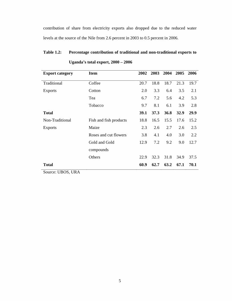
5
contribution of share from electricity exports also dropped due to the reduced water
levels at the source of the Nile from 2.6 percent in 2003 to 0.5 percent in 2006.
Table 1.2: Percentage contribution of traditional and non-traditional exports to
Uganda’s total export, 2000 – 2006
Export category Item 2002 2003 2004 2005 2006
Traditional
Exports
Coffee 20.7 18.8 18.7 21.3 19.7
Cotton 2.0 3.3 6.4 3.5 2.1
Tea 6.7 7.2 5.6 4.2 5.3
Tobacco 9.7 8.1 6.1 3.9 2.8
Total 39.1 37.3 36.8 32.9 29.9
Non-Traditional
Exports
Fish and fish products 18.8 16.5 15.5 17.6 15.2
Maize 2.3 2.6 2.7 2.6 2.5
Roses and cut flowers 3.8 4.1 4.0 3.0 2.2
Gold and Gold
compounds
12.9 7.2 9.2 9.0 12.7
Others 22.9 32.3 31.8 34.9 37.5
Total 60.9 62.7 63.2 67.1 70.1
Source: UBOS, URA
6
1.3 Trend of expenditure on Ugandan imports
Over the years, Uganda’s expenditure on imports has continued to increase at a higher
rate than proceeds from exports (UBOS, 2007). During 2006, expenditure on imports
amounted to US$ 2,557.3 million, which was about US$ 831,000 more of what was
spent in 2004. The continuous expenditure on imports is attributed to the desire to satisfy
the domestic market, which has a high demand of both capital and manufactured goods.
For the past decade, petroleum and its products, road vehicles, cereals, iron and steel
among others have been the key imports of Uganda. Petroleum products have continued
to take the highest expenditure over the years, followed by vehicles and cereals in that
order. By 2006, the import expenditure shares for petroleum and its products, road
vehicles and cereals were estimated at 20.6, 8.5 and 6.1 percent, respectively.
Other imports include telecommunications, medical and pharmaceutical products.
UBOS (2006) asserts that Asia was the largest source of Uganda’s imports. Uganda’s
expenditure on Asian imports between 2005 and 2006 increased by 38.7 percent was
attributed to China’s entry in the import market. Unlike Asia’s increased share of import
expenditure, import expenditure share for the African continent significantly reduced
from 36.2 percent in 2005 to 25 percent in 2006. Of Uganda’s import expenditure on
African imports, the Common Market for East and Southern Africa (COMESA) assumed
70.5 percent of the market share. During the past ten years, Kenya has been the major
source of imports both on the African continent and COMESA region (62.7 percent and
89 percent respectively). Other African trade partners were Republic of South Africa,
Egypt, DRC, to name but a few.
7
1.4 Uganda’s trade partners
COMESA member states and European Union (EU) countries have been the Uganda’s
leading trading partners over the years. During 2006, COMESA’s trade market share was
at 29.5 percent followed by the European Union (27.4 percent) and the Middle East with
20.6 percent. Of recent, the Middle East has emerged as a potential market given that its
market share has considerably increased by about 10 percent from 10.8 percent in 2005.
According to UBOS (2007), Kenya, Rwanda, Sudan and DRC are the major trading
partners amongst the COMESA states. From 2005, the value of exports to COMESA
region rose by 13.8 percent. Within the European Union region, Netherlands, France,
Belgium and Germany are the major trading partners. North America and Asia are other
trade partners although their overall export shares are still low staggering at 1.7 percent
and 7.8 percent, respectively. Eighty six percent of exports to North America were
destined for the USA although export values to USA decreased from US$ 15.9 million in
2005 to US$ 14.2 million in 2006.
Generally, Uganda’s bilateral trade flows have been varying from time to time as
portrayed in Appendix I. For over ten years, trade remained stagnant between the years
of 1970 and 1981, and picked up for the following ten years until the early 1990s when
there was rapid growth in trade flows. Since then, Uganda’s bilateral trade flow has
rapidly developed until to date. Uganda trades with many countries into the world but
for the 37 years considered in this study, significant trade was observed with Kenya
followed by South Africa and the Netherlands. During the late 1990s, trade with the UK
and Switzerland had begun to pick up.

8
1.5 Problem Statement
Trade is a crucial instrument for industrialization and sustainable economic development.
Traditional trade theories are mainly concerned with identifying what goods a country
trades, while ignoring the trade volumes. Understanding the factors determining bilateral
trade volumes of a country or a region widens the horizons of a country or region’s trade
policies. The gravity flow model helps to understand the factors that determine a
country’s bilateral trade volumes from a practical or empirical point of view. It broadens
the horizons of a country’s trade policies (Deardorff, 1998; Eichengrean and Irwin, 1997;
Luca and Vicarelli, 2004). Various gravity analyses are performed to evaluate various
trade policy issues, such as the effects of openness of an economy or protectionist
policies and the merits of proposed regional trade arrangements (such as COMESA and
East African Community in the case of Uganda) and the effects of national borders.
Recent empirical studies have employed the gravity model in determining patterns of
tourism flows, migration flows, bilateral equity flows and foreign direct investment
flows.
Successfully identifying the bilateral trade flows can suggest a desirable free-trading
partner and conjecture the volume of a missing trade or unrealized bilateral trade flows.
In the case of Uganda, the trade gravity model is a powerful tool for explaining the
bilateral trade flows and volumes. The trade flows and volumes can then be widely
applied to analyze the inter-national bilateral trade volumes and to estimate trade
potentials. Additionally, the model can be employed to identify the effects of trade
groups, explain the trade patterns and to assess the cost of a border trade. In trade policy
analysis, the model can widely be used as a baseline to estimate the impact of a variety
of policy issues with respect to currency unions, regional trading groups and various
9
trade distortions (Anderson, 1979; Bergstrad, 1985, 1989; Bougheas et al., 1999; Lin and
Wang, 2004; Liu and Jiang, 2002; Lin, et al., 2002; De Sousa and Disdier, 2002; Sheng
and Liao, 2004).
In Uganda, the gravity flow model has evidently been employed by Muhammad and
Andrews (2008) to investigate the determinants of tourist arrivals in Uganda. No
scholarly work has been done to assess the determinants of Uganda’s bilateral trade
flows and potential. A deeper understanding of Uganda’s bilateral trade flows would
provide an additional practical framework for making informed trade policy decisions to
improve the country’s trade regime. For transitional countries like Uganda, UNCTAD
(1999) notes that the gravity flow model is very relevant while making informed policy
decisions especially when modelling potential trade flows and examining changes among
international trading partners of transitional economies. The International Trade Centre
(ITC) (2003) reported a new modification of the ordinary Gravity flow model called
TradeSim developed purposely to estimate bilateral trade flows of developing countries
with any of their trading partner countries.
Although a lot of empirical work on bilateral trade flows has been done in developed
countries (Martinez-Zarzoso, 2003; Chen et al., 2007; Luca and Vicarelli, 2004;
Sokchea, 2006; Sheng and Liao, 2004), there is very little work in this area in Africa,
and Uganda specifically. Thus, it is against this background that this study employs the
Augmented-gravity flow model to determine factors affecting Uganda’s total bilateral
trade flows and her trade potential.

10
1.6 Objectives of the study
The main objective of this study was to determine factors affecting Uganda’s bilateral
trade flows and her trade potential. The specific objectives were:
1. To determine the factors that influence bilateral trade flows between Uganda and
her major trade partners.
2. To predict Uganda’s bilateral trade potential and performance.
3. To determine Uganda’s degree of trade integration with her major trade partners.
1.7 Hypotheses
1. Growth of real GDPs of Uganda and her major trade partners positively influence
the level of bilateral trade flows.
2. The longer the distance between Kampala city and a capital city of a major trade
partner, the lower the level of bilateral trade flow.
3. Exchange Rate Volatility and Misalignment lower the level of bilateral trade flows.
4. Uganda has a good level of trade performance with her major trade partners.
11
CHAPTER TWO
LITERATURE REVIEW
2.1 Determinants of Bilateral Trade Flows
Various studies related to international trade flows have been carried out using the
Gravity flow model approach in a number of countries. For example, Muhammad and
Andrews (2008) applied the gravity flow model and panel data for a period of five years
(2000 – 2004) to investigate the impact of origin-specific factors across countries on
tourist arrivals in Uganda. Generally, Ordinary Least Squares (OLS) results of the study
suggest that over 70 percent of the variation in Ugandan tourist inflows could be
explained by real GDP, distance, Ugandan exports by country destination, Ugandan
imports by country of origin and exchange rates. Distance was identified as the greatest
factor negatively affecting Uganda’s tourist arrivals given that for a unit percent increase
in distance from Uganda would lead to a 70 percent decrease in tourist arrivals.
Achay (2006) investigated the determinants of trade flows between various countries.
The author applied the augmented gravity flow model on a sample of 146 countries for
the five-year sub-periods between 1970 and 2000. The augmented gravity model
included the basic factors of the model, which are GDP and distance as well as other
variables which included per capita GDP, common official language, common frontier
and common currency. Results of the study indicated that GDP, GDP per capita,
common frontier, common official language, and common currency have a positive
impact on the volume of bilateral trade. On the other hand, the geographical distance
factor had a negative effect on the volume of trade.
12
According to Geda (2002) who analyzed the determinants of trade using COMESA as a
case study, documented that, with the exception of distance, all the standard gravity
model variables had plausible and statistically significant coefficients. It was noted that
good macroeconomic policies (such as financial deepening and infrastructure
development) were important determinants of bilateral trade in Africa. All proxies used
to measure political instability with the exclusion of war had the expected signs.
Regional integration arrangements were negatively influencing intra-regional trade.
COMESA intra-trade partners were found not significantly different from non COMESA
countries.
Martinez-Zarzoso (2003) applied the gravity model to assess Mercusor countries and the
European Union trade and trade potential following the trade agreements that had been
reached. The model was used to test annual bilateral trade flows on a sample of 19
countries, that is, the formal four members of Mercosur plus Chile and the fifteen
members of the European Union over a period of eight years (1988 – 1996). The basic
model variables satisfied the gravity flow model hypothesis which states that, “Economic
sizes of trading partners positively influenced bilateral trade flows while distance
between the economic trading centres of any two trading partners negatively affected
bilateral trade flows”. However, population of importing trade partners was found to
positively influence bilateral trade flows, implying that bigger countries import more
than their smaller counterparts. Also the population of the exporting country had a large
and positive impact on volume of exports. According to the author, it implies that the
larger the population, the cheaper the available labour. This boosts production of
exportable goods and services. Exporter and importer incomes also indicated a positive

13
influence in bilateral trade flows but the author’s major observation was that transport
infrastructure greatly fosters trade.
Chen et al. (2007) studied determinants of Xinjiang’s bilateral trade flows using an
extended gravity flow model. The variables “GDP product”, “the product derived from
per capita GDP of Xinjiang and that of her trade partners”, and distance among other
variables were found to be significantly consistent with the then prevailing trade
situation at the time of study. The authors noted that Xinjiang’s neighbouring trade
partners like Russia, the Republic of Kyrgyzstan and Pakistan, which have a direct land
corridor, were always Xijiang’s main trade partners unlike distant trading partners like
Hong Kong among others.
The distance variable has remained one of the most interesting simply because, different
authors give quite differing views about this variable. For instance, Buch et al. (2003),
put it that, distance coefficients do not carry much information on changes in distance
costs over time because changes in distance costs are largely picked up solely in the
constant term of the gravity model. Therefore, the distance coefficient only measures the
relative difference between economic centres. Chan-Hyun (2005) clarifies that the
distance coefficient does not only reflect elasticity of absolute distance on trade, but also
shows the effect of both absolute and relative distances.
Empirically, real exchange rate volatility can have both negative and positive effects on
trade depending risk aversion and costly adjustment of production factors. For instance,
De Grauwe, (1988) notes that risky aversion and costly adjustment of production factors
may lead to a negative impact of exchange rate volatility on exports, while convexity of
14
the profit function with respect to export prices may lead to a positive impact. However,
most studies (Thursby and Thursby, 1987; Frankel, 1997; Frankel and Wei, 1993;
Eichengreen and Irwin, 1995) have found exchange rate volatility to negatively influence
trade flows although Klein (1990) observed a positive effect. While assessing the effects
of exchange rate uncertainity on agricultural trade among the G-10 countries (Belgium,
Canada, France, Germany, Italy, Japan, the Netherlands, Switzerland, the United
Kingdom and the United States), Cho et al., (2002) concluded that exchange rate
volatility had a large negative impact on trade flows. Related work by Kandilov (2008),
who employed data for developed, emerging and developing countries between 1975 and
1997, also registered a negative effect of exchange rate volatility on export trade most
profoundly among the developing economies. According to Kandilov (2008), most
existing studies that evaluate the impact of increased exchange rate volatility on trade
flows are for developed economies, yet many developing economies in Asia, South
America and Africa in particular, pursue GDP growth policies based on trade orientation.
Thus, the question of real exchange rate volatility on bilateral trade flows specifically in
Uganda is the information gap of importance as per this variable.
Gue et al., (2003) who used the gravity flow model following Bergstrand (1985, 1989)
and Feenstra et al. (2001) puts it that, over-valuation (under-valuation) of the nominal
exchange rate negatively (positively) affects export performance, particularly to the
agricultural sector. The study sought to address the effect of exchange rate misalignment
on agricultural trade in comparison with its impact on other sectors. It was based on
panel data for 10 developed economies compiled over a period of 25 years (1974-1999).
Findings of the study show that exchange rate misalignment greatly decreases (- 1.116)
agricultural trade flows unlike the case with the other sectors. This implied that a unit
15
change in nominal exchange rate misalignment (over- or under-) valuation of a currency
compared to the long-run equilibrium level influences (reduces or increases) agricultural
trade flows by about 1.1 percent although other sectors like the large-scale
manufacturing were not significantly affected. Despite the fact that previous studies have
assessed the impact of exchange rates on trade, many (Gue et al., 2003; Gardner, 1981;
and Tweeten, 1989) have used nominal exchange rate instead of using real exchange
rates; hence real exchange rate misalignment is a key research concern in this study.
Most of the literature reviewed shows that GDP coefficient lies between 0.75 and 1.2,
which is consistent with the theoretical foundation (Grossman, 1998; Deardorff, 1998).
Many scholars (Frankel, 1997; Chen et al., 2007; Chan-Hyun, 2005) also proved this
assertion by carrying out a number of gravity equations and the results showed that
coefficient for real GDP ranged between 0.75 and 0.95. However, contrary to the
theoretical expectations, Sokchea (2006) obtained statistically significant GDP
coefficients even when random effects were catered for in the estimator. When the OLS
estimator was used, coefficients ranged between 2.188 and 3.178 across the study
periods, which is more than the theoretical value of 1.2. Use of the Simple pooled OLS
estimator also gave a wide range of coefficients lying between 2.585 and 5.851. With
respect to GDP variable, this study seeks to validate whether GDP of Uganda and her
trade partner’s lies within the expectations of the theoretical foundation.
2.2 Determination of Bilateral Trade Potential
Studies by Luca and Vicarelli (2004), Martinez-Zarzoso (2003) and Kalbasi (2004)
carried out basing on the gravity flow model framework have tried to predict bilateral
trade potentials. In essence, these studies seek to acquire evidence of effects that arise
when countries have been integrated in trade so that they can predict the additional
16
bilateral trade flows that might accrue if there is any kind of fostering trade integration
between two or more countries (Luca and Vicarelli, 2004). Martinez-Zarzoso (2003)
used the estimated coefficients obtained from the gravity flow model to predict
Mercosur’s export potential to the European Union (EU). Results from the study show
that teaming up of Mercosur and Chile provided the highest export potential (approx.
22.6 million) to the EU while Paraguay registered the least export potential (approx.
231,000) to the EU for the entire study period (1988-1996). This implies that Mercosur
and Chile have more room to expand their trade to the EU unlike Paraguay.
Kalbasi (2004) also used a similar approach to predict Iran’s total export trade flow
potential to the 76 trade partner countries in 1998. In the analysis, the author categorized
the export trade flows into two categories, that is, the developing – industrial countries
(DI) and the Intra-developing countries (DD) export trade flows. Findings of the study
reveal that of the DI countries export trade flows, United States of America (USA) and
Japan had the highest export trade flow potential while Greece, New Zealand and Ireland
trailed at the bottom. Among the DD countries export trade flows, Turkey and Pakistan
registered the highest export trade flow potential while Argentina, Venezuela, Tunisia
among others had very low export trade flow potentials. Most of the countries in this
category actually registered zero export trade flow potential. While comparing results of
the different gravity flow model estimators (the traditional static OLS, fixed effects
regression and the dynamic specification), Luca and Vicarelli (2004) also predicted trade
potentials. Results indicated that predicted trade potentials vary when one uses the
different gravity flow model estimators. Authors further noted that the predicted trade
potentials decrease as one uses the traditional static OLS, followed by the fixed effects
regression and then the dynamic specification in that order.
17
2.3 Analysis of Trade Performance and Degree of Trade Integration
Although many gravity flow model empirical studies have been conducted on
determinants of bilateral trade flows, not much literature review related to analysis of
trade performance and Degree of trade integration has been come across. According to
Chen et al. (2007) who used 34 countries to quantitatively analyze Xiniang’s trade
performance in 2004, there are two indices, which can appropriately be used to as good
measures of trade performance. These are Relative difference (Rd) and Absolute
difference (Ad). Their results revealed that Xinjiang had good trading terms with most of
her trading partners given that the Rd was above zero. Kazakhstan, Pakistan, Germany,
Russia and France, among others, were particularly good trading partners with Xinjiang
given that their respective Rd indices ranged between 0.35 and 0.60. However, some
trading partners like Greece, Iran and Norway had Rd indices far below zero (between -
0.79 and -0.10) which implied that those partners were not by then cooperating with
Xinjiang.
As per the Absolute difference (Ad) index, Chen et al. (2007) based their analysis on
geographical regions. Results of the study showed that, Xinjiang had already established
strong trade ties with Central Asia, Central and Eastern Europe, and Western Europe.
She had gained from her trade with Central Asia (US$ 900 million), Central and Eastern
Europe (US$ 100million) and Western Europe (US$ 80 million) unlike with other
regions like West and South Asia which had had trade volume gains worth less than US$
30 million only. Xinjiang’s good regional trade performance with Central Asia, Central
and Eastern Europe, and Western Europe was attributed to the existence of a number of
common aspects like culture, customs and religious beliefs, and the having of traditional
economic exchanges. In particular, authors noted that central Asia has the new Eurasian

18
continental bridge and many land ports, which made the study country the “bridgehead”
in opening up westwards.
To measure a Korea’s degree of trade integration, Chan-Hyun (2005) used the ratio of
actual trade to potential trade and empirical results from Korea and her 30 major trading
partners revealed that China, Japan and Mexico had significant trade barriers. These
barriers could have led to the great levels of unexhausted trade potential of about 3,178
(China); 23,163 (Japan) and 2,840 (Mexico) billion US dollars. This assertion was
attributed to relatively lower ratios 0.85 (China), 0.67 (Japan) and 0.29 (Mexico)
obtained. Sandra (2006) used dummy variables with the gravity flow model of trade to
investigate the evolution of Yunnan’s international trade integration between 1988 and
1999 with a sample of 230 observations. The study focused on assessing the impact of
membership to the Great Mekong Sub-region (GMS). Results showed that a large degree
of trade integration existed between Yunnan and Myanmar for both imports and exports.
However, Yunnan depicted a negative degree of trade integration with Thailand and
Vietnam implying no existence of good trading terms.

19
CHAPTER THREE
METHODOLGY
3.1 Study area
The study focuses on Uganda’s seven main trade partners (Switzerland, Belgium,
Netherlands, Kenya, South Africa, United Kingdom and France). They were selected
basing on the fact that they have been consistent trading partners over the past ten years
and have high percentage contribution to total bilateral trade flow with Uganda. Two
market integration systems were considered, that is, membership to COMESA and the
East African Community (EAC). Kenya and South Africa are members to COMESA,
and Kenya also belongs to the East African Community (EAC). The market integration
systems represent the dummy variables in the specified augmented gravity model.
3.2 Data description and data analysis
This study concentrates on panel data collected over a period of 37 years (1970 – 2006).
This period was selected because the study intends to track the evolution of Uganda’s
trade partners and to maintain the comparability of the estimated coefficients. The study
uses International Financial Statistics (IFS) database of 1998 and 2007 developed by
International Monetary Fund (IMF). The IFS provides yearly statistical data classified
according to international standards. Other data sources include the annual Statistical
Abstract publications (since the 1980s) by the Uganda Bureau of Statistics and the
United Nations Statistics Division Common Database for the 37 years covered by this
study.

20
Bilateral trade by value (imports and exports) by trade partner countries, Nominal GDP
at current market prices, Real GDP at constant prices of 1990, United states producer
prices, Uganda’s consumer price index, Population of Uganda and her trading partners
were taken from the IFS (IMF, 1998; 2007) and from the United Nations Statistics
Division Common Database. United Nations’ GDP estimates were used because the
figures were given in a uniform and an internationally recognised dollar currency unlike
the IMF figures that were reported in the respective national currencies. Distance data
are the air distances between the capital cities (Economic centres) of selected trade
partners with reference from Kampala, Uganda. These data were taken from
www.mapcrow.info/distance and www.worldatlas.com
The data were entered, coded and cleaned in Statistical Package for Social Scientists
(SPSS) computer program. A summary of descriptive statistics such as percentages,
means, standard deviations and t-statistics were generated. The data were then
transferred to STATA version 9.0 in which empirical analysis was carried out. Total
bilateral trade variable was obtained as a summation of Uganda’s exports and imports to
(from) each of the trading partners. With the exception of the dummy variables, the
natural logarithms of the other variables, that is, total bilateral trade, real GDP,
population and distance were also generated. In the econometric analysis, nine variables
were examined for eight trading partners, Uganda inclusive. This gave a panel of 259
observations.
21
3.3 Analytical methods
3.3.1 Model Specification for the Augmented-Gravity Flow Model
Over the last four decades, the gravity flow model has become a popular formulation for
statistical analysis used to predict bilateral trade flows between different geographical
entities basing on the economic sizes of the different locations or countries, specifically
using GDP measurements (Bergstrand, 1985, 1989; Deardorff, 1998; Eichengrean and
Irwin, 1997; Luca and Vicarelli, 2004). The model originates from Newton’s “Law of
Universal Gravitation” proposed in 1687 (Keith, 2003). It holds that the attractive force
between two objects i and j is a positive function of their respective masses (M i and Mj)
and a negative function of the distance (Dij) between them. This attraction is given by:
(1)
= 2
D ijM jM iGFij
Where Fij is the attractive force, Mi and Mj are the masses, Dij is the distance between the
two objects and G is a gravitational constant depending on the units of measurement for
mass and force.
In international economics, the basic gravity flow model states that the size of trade
flows between two countries is determined by supply conditions at the origin, demand
conditions at the destination and stimulating or restraining forces related to the trade
flows between the two countries (Keith, 2003). This can be shown as
(2)
Dij
jMiMRFij θ
βα
*=
Where Fij is the trade flow from origin і to destination j, Mi is the economic mass (GDP)
of exporting country, Mj is the economic mass (GDP) of the other trading partner. D is
22
the distance between the commercial centers of the two countries and R (Remoteness)
replaces the gravitational constant G. Given the multiplicative nature of the model,
natural logarithms can be taken to obtain the linear relationship as stated in equation (3).
(3) ερθβα ijR jDijM jM iFij ++−+= lnlnlnlnln
The augmented-gravity flow model can be expressed as specified below (Foldvari,
2000):
(4) εργδθβα ijR jP jP jDijM jM iFij ++++−+= lnlnlnlnlnlnln
Where Pi and Pj are the populations of country i and j, respectively.
Chen et al. (2007) and Keith (2003) assert that many other factors also influence the
trade flows among trade partners, such as the exchange rate, export tax and tariffs, which
are controlled by governments and their agencies among others. Other factors include
membership in trade arrangements, such as the European Union, COMESA and the
NAFTA, EAC, PTA, etc. Whalley (1998) puts it that member states get more economic
benefits from guaranteed markets within trade groups than in others. In order to analyse
the effects of regional integration on trade volumes, dummy variables are used to capture
such trading blocs. In addition, cultural ties such as colonial relationship between
Uganda and United Kingdom can be captured using a dummy variable. Thus, Uganda’s
determinants of bilateral trade flows were obtained by running an augmented-gravity
flow model while using the Feasible Generalised Least Squares (FGLS).
The FGLS estimator assumes that heteroscedasticity to be panel as expressed as in (5).
(5)εββββββ
ββββα
ijDUKDEACDCOMESAMisalignitVolitDistij
OtherpopjtUgpopitOthergdpjtUggdpitijTradeUgijt
+++++++
++++=
108 97ln6ln5
4ln3ln2ln1ln
23
where lnTtradeUgijt is total bilateral trade (sum of exports and imports) between
Uganda and her j th trading partner in year t in Billions of US Dollars; lnUggdpit is real
GDP of Uganda in year t in Billions of US Dollars; lnOthergdpjt is real GDP of the j th
trading partner in year t in Billions of US Dollars; lnUgpopit is Uganda’s population in
year t in millions; lnOtherpopjt is jth trading partners’ population in year t in millions;
lnDistij is distance between Kampala and her jth trading partner’s commercial centre in
Miles, lnvolit is real exchange rate volatility, Misalignit is the real exchange rate
misalignment, DCOMESA is a dummy variable representing the influence of
membership in COMESA (= 1, if country was in COMESA and at a given year t and =
0, if otherwise); DEAC is a dummy variable representing the effect of membership in
East African Community (=1 if country was in EAC in a given year and = 0 otherwise);
DUK is a dummy variable representing the effect of colonial ties to Britain (=1 for UK
as trade partner and = 0 otherwise). The set hypotheses were tested using the t-statistic in
comparison with the significance levels.
3.3.2 Variables and Expected signs of the coefficients
Real Gross Domestic Product (GDP): GDP of the trading countries represents both the
productive and consumption capacity that determines largely the trade flow among them.
The Real GDPs are used to proxy for the economic sizes of the countries and it is
expected that an importing country’s GDP plays a significant role in determining the
trade flow originating from exporting countries. This is because the importing country’s
GDP, like the income of the consumer, determines the demand for the goods originating
from exporting countries. An exporting country’s real GDP also helps in ascertaining
productive capacity of the exporting country, that is, the amount of the goods that could
be supplied. In the gravity model, it is expected that an exporting country’s GDP
influences the trade flow of goods and services originating from the exporting country.

24
Thus, as real GDP of any two or more trading countries increases, trade flows also
increase. Therefore, the coefficients of Real GDPs are expected to be positive.
Distance (distij) is another important variable, which is used to capture the proxy for the
trade cost between countries. Distance is a trading resistance factor that represents trade
barriers such as transportation costs, delivery time, cultural unfamiliarity and market
access barriers. Among other factors, higher transportation costs reduce the volume of
trade and increase information costs. Countries with short distance between each other
are expected to trade more than those who are wide apart because of reduced transaction
costs. Distance can also be used as a proxy for the risks associated with the quality of
some of the goods and the cost of the personal contact between managers and customers.
Despite the cardinal “great circle” formula which approximates the earth’s shape as a
sphere and calculates the minimum distance along the surface, distance were obtained
using the geographical distance. Following Giorgio (2004) and Keith (2003), this was
intended to avoid the short comings associated with the “great circle” formula.
Generally, the coefficient of distance is expected to negatively influence the flow of
trade between countries.
Population: The impact of Uganda’s population and that of her trading partners were the
other factors considered. Population is used as measure of country size, and since larger
countries have more diversified production and tend to be more self sufficient, it is
normally expected to be negatively related to trade.
Real exchange rate volatility: Among other variables considered in this study, was Real
Exchange rate volatility given that it can affect trade both directly and indirectly. Direct
effects are can be through uncertainty and adjustment costs, while indirect effects can be
through its influence on the structure of output and investment and on government policy

25
(Cote, 1994). The consequences of exchange rate volatility on trade have long been at
the centre of the debate on the optimality of alternative exchange rate regimes.
Proponents of fixed rates argue that since the advent of the floating regime, exchange
rates have been subject to excessive volatility and deviations from equilibrium values
have persisted over sustained periods of time. In their view, exchange rate volatility
deters industries from engaging in international trade and compromises progress in trade
negotiations.
In contrast, proponents of flexible rates argue that exchange rates are mainly driven by
fundamentals, and that changes in fundamentals would require similar, but more abrupt,
movements in fixed parities. Real exchange rate volatility was measured using the
standard deviation (or variance) approach as expressed in equation (6) below.
(6) ( ) 2^ℜ−= RVol itit
Where Volit denotes Uganda’s real exchange rate volatility, Rit represents real
equilibrium exchange rate and ℜ denotes mean annual exchange rate. The coefficient of
Real exchange rate volatility is expected to have a negative sign.
Real exchange rate misalignment: Generally, the term misalignment refers to the
departure of nominal exchange rates from long-run equilibrium level or market
fundamentals such as relative prices and interest rate differentials between countries
(Gue et al., 2003). It can be characterized as either over- or under-valuation of the
currency relative to fundamentals. According to it is difficult and inherently imprecise to
measure misalignment, given that it requires estimation of what is termed as the
fundamental equilibrium exchange rate. The variable was calculated basing on the
26
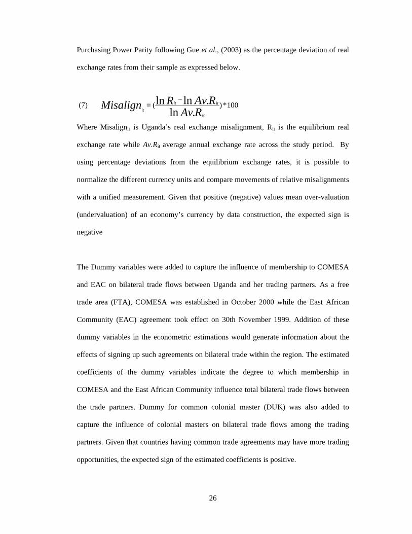
Purchasing Power Parity following Gue et al., (2003) as the percentage deviation of real
exchange rates from their sample as expressed below.
(7) 100*)(.ln
.lnlnRAv
RAvRMisalignit
itit
it
−=
Where Misalignit is Uganda’s real exchange misalignment, Rit is the equilibrium real
exchange rate while Av.Rit average annual exchange rate across the study period. By
using percentage deviations from the equilibrium exchange rates, it is possible to
normalize the different currency units and compare movements of relative misalignments
with a unified measurement. Given that positive (negative) values mean over-valuation
(undervaluation) of an economy’s currency by data construction, the expected sign is
negative
The Dummy variables were added to capture the influence of membership to COMESA
and EAC on bilateral trade flows between Uganda and her trading partners. As a free
trade area (FTA), COMESA was established in October 2000 while the East African
Community (EAC) agreement took effect on 30th November 1999. Addition of these
dummy variables in the econometric estimations would generate information about the
effects of signing up such agreements on bilateral trade within the region. The estimated
coefficients of the dummy variables indicate the degree to which membership in
COMESA and the East African Community influence total bilateral trade flows between
the trade partners. Dummy for common colonial master (DUK) was also added to
capture the influence of colonial masters on bilateral trade flows among the trading
partners. Given that countries having common trade agreements may have more trading
opportunities, the expected sign of the estimated coefficients is positive.

27
3.3.3 Predicting Bilateral Trade Potential and Performance
Over the years, two main approaches have been used to calculate bilateral trade potential,
that is, the out of sample approach and the in-sample approach. However, this particular
study employs the out of sample approach to predict Uganda’s potential bilateral trade
flows as specified in (8).
(8)εββββββ
ββββα
ijDUKDEACDCOMESAMisalignitVolitDistij
OtherpopjtUgpopitOthergdpjtUggdpitijTradeUgijt
+++++++
++++=
108 97ln6ln5
4ln3ln2ln1ln
Where β0 denotes the constant and β1- β8 represent coefficients of the variables earlier
defined.
With this approach the exact parameters estimated by the gravity flow model were used
to project the “natural” trade relations between the trading partners such that the
difference between the actual and predicted trade flows represent the un-exhausted trade
potential (Wang and Winters, 1992; Hamilton and Winters, 1992; and Brulhart and
Kelly, 1999). According to Baldwin (1994) and Nilsson (2000), the second approach (in-
sample approach) derives trade potential estimates from within the sample. This means
that residuals of the estimated regression are taken to represent the difference between
potential and actual trade relations. Notably, Egger (2000) and Luca and Vicarelli (2004)
argue that both approaches can not be considered immune from eventuality of serious
bias, especially if there is model misspecification. However, ITC (2003) confidently
notes what matters most is the sign of the difference between potential and actual trade
flows.

28
Following Lie et al., (2002), Amita (2004) and Jiang et al., (2003) bilateral trade
performance was analysed using two indices, that is, the Relative difference (Rd) and
Absolute difference (Ad) following. To obtain the Relative difference (Rd) index
expressed in equation (9), the mean simulated (potential) trade value together with the
mean actual trade value was used as;
(9) ( )( ) 100*
TijtAijt
TijtAijtRdijt
+
−=
Where Rdijt denotes relative difference in Uganda’s with trade partner j. Aijt denotes
mean actual trade and Tijt is the mean simulated trade. Lie et al., (2002) and Jiang et al.,
(2003) assert that Rd is inspired by the Normalized Difference Vegetation Index (NDVI)
and it varies between -1 and 1. That is, -1.0 ≤ Rd ≥ 1.0. Rd is used to measure the good
or bad trade performance between trade partners and to analyse exporter’s future trade
direction given the present circumstances (Chen et al., 2007). The larger the Rdijt is, the
more successful the bilateral trade cooperation is although (Amita, 2004; Helmers and
Pasteels, 2003) note that bilateral trade should be enhanced in advance. With this index,
trade performance was analysed at four stages, that is, i) while considering the entire
study period of 37 years, ii) when considering the period between 1990 and 2006, iii) for
the period from 1995 to 2006, and iv) between 2000 and 2006.
29
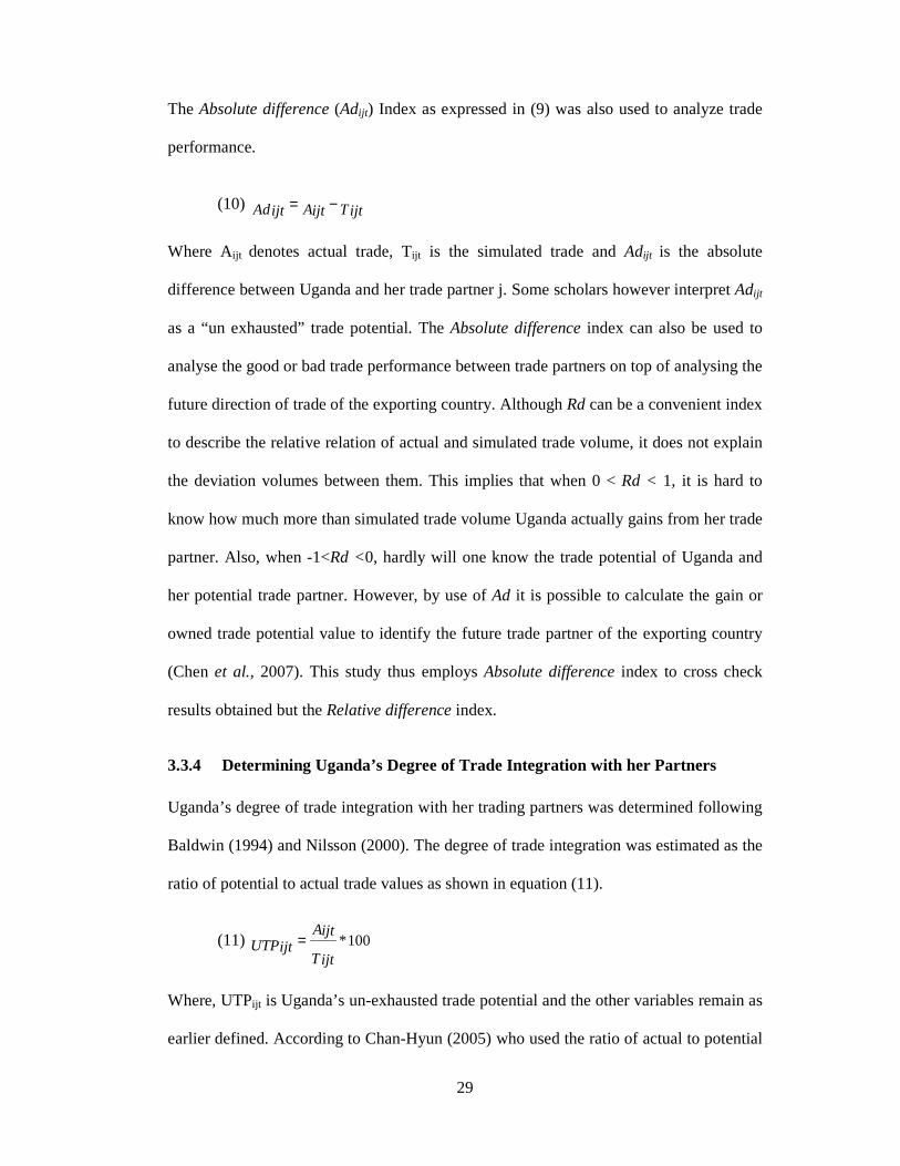
The Absolute difference (Adijt) Index as expressed in (9) was also used to analyze trade
performance.
(10) TijtAijtAdijt −=
Where Aijt denotes actual trade, Tijt is the simulated trade and Adijt is the absolute
difference between Uganda and her trade partner j. Some scholars however interpret Adijt
as a “un exhausted” trade potential. The Absolute difference index can also be used to
analyse the good or bad trade performance between trade partners on top of analysing the
future direction of trade of the exporting country. Although Rd can be a convenient index
to describe the relative relation of actual and simulated trade volume, it does not explain
the deviation volumes between them. This implies that when 0 < Rd < 1, it is hard to
know how much more than simulated trade volume Uganda actually gains from her trade
partner. Also, when -1<Rd <0, hardly will one know the trade potential of Uganda and
her potential trade partner. However, by use of Ad it is possible to calculate the gain or
owned trade potential value to identify the future trade partner of the exporting country
(Chen et al., 2007). This study thus employs Absolute difference index to cross check
results obtained but the Relative difference index.
3.3.4 Determining Uganda’s Degree of Trade Integration with her Partners
Uganda’s degree of trade integration with her trading partners was determined following
Baldwin (1994) and Nilsson (2000). The degree of trade integration was estimated as the
ratio of potential to actual trade values as shown in equation (11).
(11) 100*Tijt
AijtUTPijt =
Where, UTPijt is Uganda’s un-exhausted trade potential and the other variables remain as
earlier defined. According to Chan-Hyun (2005) who used the ratio of actual to potential

30
trade to estimate the un-exhausted trade potential, trading partners with relatively lower
ratios can not easily be integrated in trade hence causing a considerable level of un-
exhausted trade potentials.
The degree of trade integration was also analysed while using the coefficients on
Dummy variables (dcomesa and deac) as specified in equation (12).
(12) Degree of trade integration = [(exponent (dummy coefficient)) – 1] * 100
= [(2.718281828^ (dummy coefficient))-1)*100
This approach is based on assessing the effectiveness COMESA and the East African
Community (EAC) on Uganda’s trade flows. The method follows CPD (2006) and
Sandra (2006) who note that a positive and statistically significant coefficient on the
dummy variables implies that trade flows exceed the normal level, meaning that there is
greater economic trade integration. However, when the coefficient is statistically
negative, it means that the trade flows fall short of the predicted volume, thereby
signifying a low degree of trade integration.
31
CHAPTER FOUR
RESULTS AND DISCUSSION
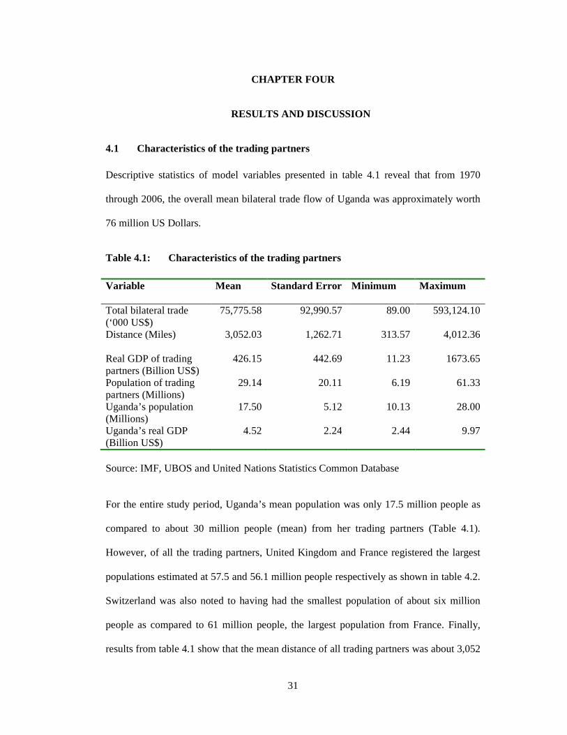
4.1 Characteristics of the trading partners
Descriptive statistics of model variables presented in table 4.1 reveal that from 1970
through 2006, the overall mean bilateral trade flow of Uganda was approximately worth
76 million US Dollars.
Table 4.1: Characteristics of the trading partners
Variable Mean Standard Error Minimum Maximum
Total bilateral trade (‘000 US$)
75,775.58 92,990.57 89.00 593,124.10
Distance (Miles) 3,052.03 1,262.71 313.57 4,012.36
Real GDP of trading partners (Billion US$)
426.15 442.69 11.23 1673.65
Population of trading partners (Millions)
29.14 20.11 6.19 61.33
Uganda’s population (Millions)
17.50 5.12 10.13 28.00
Uganda’s real GDP (Billion US$)
4.52 2.24 2.44 9.97
Source: IMF, UBOS and United Nations Statistics Common Database
For the entire study period, Uganda’s mean population was only 17.5 million people as
compared to about 30 million people (mean) from her trading partners (Table 4.1).
However, of all the trading partners, United Kingdom and France registered the largest
populations estimated at 57.5 and 56.1 million people respectively as shown in table 4.2.
Switzerland was also noted to having had the smallest population of about six million
people as compared to 61 million people, the largest population from France. Finally,
results from table 4.1 show that the mean distance of all trading partners was about 3,052

32
miles away from Kampala, Uganda’s capital city. Nairobi (Kenya) is the closest trading
partner at 313.57 miles away from Kampala while London (UK) and Amsterdam
(Netherlands) are the most distant trading centres at approximately 4,012 and 3,932
miles away from Kampala respectively.
Table 4.2 shows that over the years, Kenya had the greatest bilateral trade with Uganda
worth more than 200 million US Dollars while Belgium registered the lowest bilateral
trade worth about 28 million US Dollars only.
Table 4.2: Characteristics of Uganda and her trading partners Variable/
Country
Uganda Switzer-
land
Nether-
lands
Belgium UK Kenya South
Africa
France
Real GDP
(US$
billion)
4.5
220.8
300.8
194.1
962.3
9.8
109.5
1,172.1
Population
(millions)
17.5 6.7 14.8 10.0 57.5 23.4 35.4 56.1
Source: IMF, UBOS and United Nations Statistics Common Database
Uganda had the least real GDP of about 4.5 billion US Dollars while France and the
United Kingdom had the largest real GDP of over 1,000 and 900 billion US Dollars
respectively. Overall, the mean real GDP for Uganda’s trade partners was 426 billion US
Dollars with the highest from France (1,674 billion US$).
33
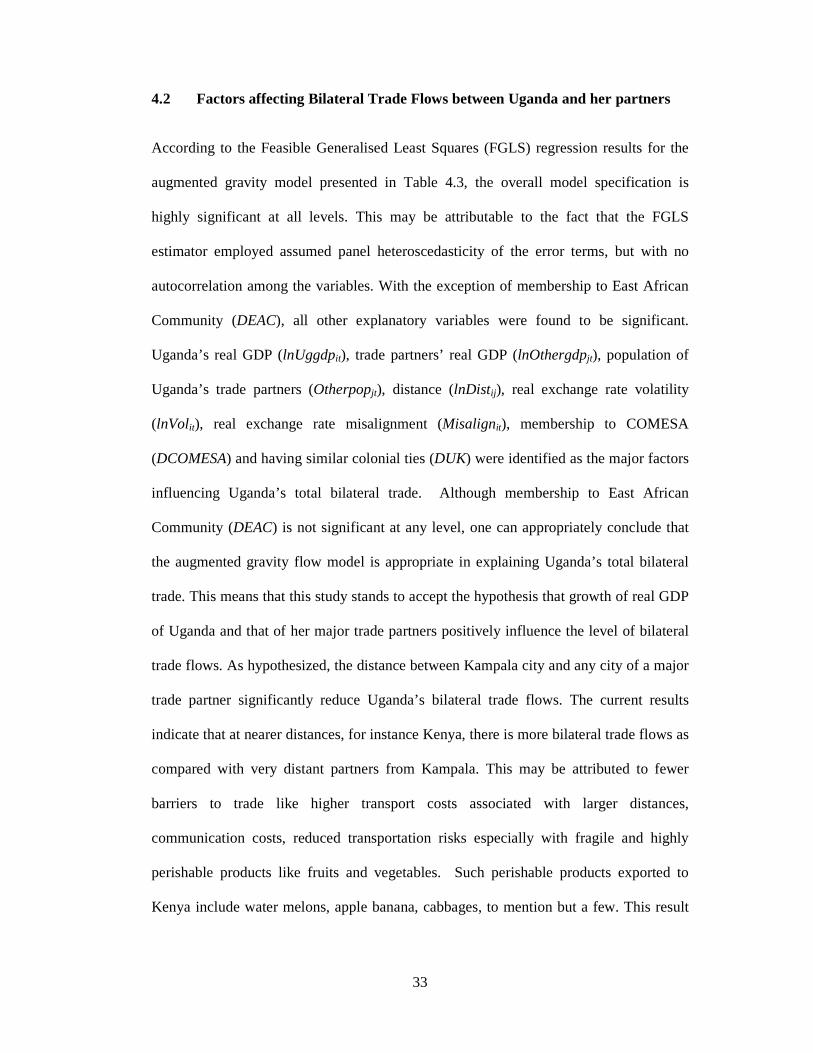
4.2 Factors affecting Bilateral Trade Flows between Uganda and her partners
According to the Feasible Generalised Least Squares (FGLS) regression results for the
augmented gravity model presented in Table 4.3, the overall model specification is
highly significant at all levels. This may be attributable to the fact that the FGLS
estimator employed assumed panel heteroscedasticity of the error terms, but with no
autocorrelation among the variables. With the exception of membership to East African
Community (DEAC), all other explanatory variables were found to be significant.
Uganda’s real GDP (lnUggdpit), trade partners’ real GDP (lnOthergdpjt), population of
Uganda’s trade partners (Otherpopjt), distance (lnDistij), real exchange rate volatility
(lnVolit), real exchange rate misalignment (Misalignit), membership to COMESA
(DCOMESA) and having similar colonial ties (DUK) were identified as the major factors
influencing Uganda’s total bilateral trade. Although membership to East African
Community (DEAC) is not significant at any level, one can appropriately conclude that
the augmented gravity flow model is appropriate in explaining Uganda’s total bilateral
trade. This means that this study stands to accept the hypothesis that growth of real GDP
of Uganda and that of her major trade partners positively influence the level of bilateral
trade flows. As hypothesized, the distance between Kampala city and any city of a major
trade partner significantly reduce Uganda’s bilateral trade flows. The current results
indicate that at nearer distances, for instance Kenya, there is more bilateral trade flows as
compared with very distant partners from Kampala. This may be attributed to fewer
barriers to trade like higher transport costs associated with larger distances,
communication costs, reduced transportation risks especially with fragile and highly
perishable products like fruits and vegetables. Such perishable products exported to
Kenya include water melons, apple banana, cabbages, to mention but a few. This result

34
generally concurs with findings of many other countries (Chan-Hyun, 2005; Kalbasi,
2004; Sokchea, 2006; Inmaculada and Felicitas, 1998; and Giorgio, 2004).
Table 4.3: Regression results of the Augmented Gravity model
Explanatory variables FGLS coefficient
Standard
error
t-
Value
P-
Value
Constant 20.91 1.499 13.95 0.000
Real GDP of Uganda (Billions US$)
(lnUggdpit)
0.736 0.228 3.22
0.001
Real GDP of the jth trading partner(Billions
US$) (lnOthergdpjt)
0.643 0.163 3.93 0.000
Uganda’s population in year t (Millions)
(lnUgpopit)
-0.603 0.323 -1.87 0.062
Population of jth trading partner in year t
(Millions) (lnOtherpopjt)
-0.443 0.166 -2.71 0.007
Distance between Kampala and her jth
trading partner’s commercial centre (Miles)
(lnDistij)
-1.439 0.193 -7.47 0.000
Real exchange rate volatility (lnVolit)) -0.071 0.025 -2.87 0.004
Real exchange rate misalignment
(Misalignit)
-0.003 0.001 -2.39 0.017
Dummy for membership to COMESA
(DCOMESA)
0.834 0.330 2.52 0.012
Dummy for membership to East African
Community (DEAC)
0.002 0.309 0.01 0.995
Dummy for colonial ties to Britain (DUK) 1.508 0.137 11.04 0.000
No. of observations 259
Wald Chi2 659.63
Log likelihood -262.25
McFadden’s Adjusted R2 0.442
The coefficient on Uganda’s real GDP has a positive value (0.736) with a very high
statistical significance at all levels. This result is consistent with the basic hypothesis of
35
the gravity flow model that trade volumes increase with an increase in a country’s
economic size. The coefficient shows that holding other variables constant, a unit
increase in Uganda’s GDP will result in 0.74 percentage increase in Uganda’s bilateral
trade flows. Results suggest that if Uganda’s economy is to develop through bilateral
trade, more investment in a number of sectors like tourism, and infrastructure
development, still remains desired to cause fast growth in the country’s GDP.
As hypothesised, the coefficient on the trading partner’s real GDP shows a highly
significant positive value of 0.643 which suggests that a unit increase in trading partner’s
real GDP leads to a 0.64 percentage increase in Uganda’s bilateral trade flows. This may
be attributed to the fact that Uganda is still one of those countries known for organically
produced foodstuffs. So, as the trading partners’ real GDPs increase, more imports in
form of agricultural foodstuffs and raw materials are obtained from Uganda. The
empirical results imply that Uganda’s bilateral trade flows approximately increase
proportionally with an increase in real GDP. These empirical findings closely concur
with Chan-Hyun (2005), Kalbasi (2004), Sokchea (2006), Inmaculada and Felicitas
(1998) and Giorgio (2004) who found out that increase in GDP of trading partner
positively influences trade flows in a domestic country.
Empirical results of this study show that the growth of Uganda’s population has a
negative effect on the bilateral trade flow. Population growth by one million people
would lead to a 0.60 percentage fall in trade flows with her major trade partners. This
reduction in the trade flows can be explained by the fact that the population of Uganda is
still in a dynamic stage of growth, that is, she is an emerging or developing country with
a continuously changing population. This means that the population is not yet stable as
36
compared to that of developed countries. Therefore, although population growth can be
associated with provision of cheaper labour force to the economy for the production of
goods and services that could be traded, the nation may not be in position to cater for the
large population size.
Uganda’s failure to cater for the large population size in the long-run leads to a minimum
efficient scale of production and less motivation in international trade as compared to a
developed country with a small population size that is well facilitated. In this context,
inefficiency and lack of motivation may be due to the fact that the large population size
may have abundant human resource and capital that may only be adequate to produce
enough products to sustain the economy without necessarily indulging in international
trade. Implicitly, results suggest that for Uganda to boost her bilateral trade flows, birth
rates should be controlled so that the country can have a small but well motivated
population that can enhance her bilateral trade. Motivation may be in form of provision
of good public infrastructure, education and credit schemes among others. These
empirical findings were however found not to be statistically significant, thus implying
that an increase in Uganda’s population may necessarily not deter growth in Uganda’s
bilateral trade flows. Study findings concur with results of Bergstrand (1989), who noted
that a negative influence a country’s population on bilateral trade flows might be due to
the labor (capital) intensive nature of goods and services, thereby discouraging citizens
from investing in trade.
Results on the influence of the population of Uganda’s trade partners reveal that an
increase in the partners’ population by one unit leads to 0.44 percent decline in the trend
of flow of goods and services with other countries. This finding is significant at all levels
37
and it is in line with the theoretical expectation. Ideally, one would argue that population
growth in an importing country creates more market for the exporting country but in the
case of Uganda, it is the contrary. The negative relationship between trade flow and trade
partners’ population can be attributed to a condition referred to as exporter substitution
effect. That is, as the population of trade partner countries grows bigger, people work
harder to provide for their own domestic market demands.
Inevitably, people’s hard work to provide for their domestic market requirements
compromises with the quantities goods and services that such a trading partner would
have other wise imported from other trading partners. If in any case, Uganda’s trading
partner were also a developing country like Kenya, then the decrease in bilateral trade
flows with such a partner would be attributed to the increased population, which makes
the then available resources scarcer such that people can no longer afford to trade with
Uganda. This would obviously lead to a fall in the overall trade volumes. No literature
has been come across trying to argue it this way; therefore, more research may be
required to qualify this argument. These empirical findings identify with findings of
Giorgio (2004) among other scholars that the bigger the population of the trading
partner, the larger the production for the domestic market.
Distance has a negative influence on Uganda’s total bilateral trade flows. A unit increase
in distance between any two economic centres was found to lead to a 1.37 decrease in
total bilateral trade flows. The negative relationship between trade and distance may be
attributed to the trade barriers, which arise as the trading partners become more dispersed
thus limiting bilateral trade. Such barriers to trade include high transport costs and
Uganda being a landlocked country. For Uganda’s case, this can be attributed to one or
38
two pertinent issues. Firstly, Uganda is a landlocked country only limited to Mombasa
port through which she can reach the rest of the world. Although there are other ports
(like Dar es Salaam in Tanzania and Boma in the Democratic Republic of Congo)
through which trade could be conducted, Uganda has over the years relied on trading
through Mombasa in Kenya. So this big disincentive to Uganda’s economy as this
aggravates the problem of landlocked ness if we cannot maximally utilize trade through
the different port outlets.
Given the other means of transport (Air and Railway), one would probably argue that
distance should not affect our trade but in the actual sense, air and railway means of
transport are either too costly to sustain profitable trade flows, particularly air transport
or defunct. Having only one small international airport (Entebbe International airport)
through which cargo planes could ease the difficulty encountered while undertaking
cross boarder distant trade is another factor that magnifies and qualifies distance to be a
negatively significant factor in Uganda’s trade flows. Given the small size of the only
international airport, fewer flights are registered per day and mostly passengers’ instead
of cargo flights. The cheap railway network through which much of the bulky tradable
goods could be transported is not solely reliable given that it does not reach many areas
in the country, particularly, agriculture production areas. However, it should be noted
that the estimated coefficients turned out to be similar to those estimated in other
previous studies of Wall, (1999); Buch et al., (2003) and Fankel, (1997) among others
even when those studies used cross sectional data unlike this particular study.
As hypothesised, real exchange rate volatility has negative influence on Uganda’s
bilateral trade flows. Findings reveal that a unit change in real exchange rate uncertainty

39
leads to a 71 percent drop in bilateral trade flows between Uganda and her trade partners.
Empirical results may be attributed to the fact that Uganda’s trade, especially exports are
dominated by agricultural commodities, which Kandilov (2008) notes to be very
sensitive to exchange rate volatility. Notably, over the years, agricultural contribution to
total exports has been high, varying between 70.4 and 48 percent since 2001. For
example, during 2002, traditional exports (Coffee, Tea and Tobacco) alone accounted for
39.1 percent of total exports with coffee contributing about 21 percent to total exports.
During 2006 and 2007, the share of traditional exports stagnated at 29.9 percent
compared to 37.3 percent recorded in 2003. Among the non traditional exports, fish has
the highest contribution to total exports, estimated at 18 percent by 2005 (UBOS, 2006;
2008). Kandilov (2008) puts it that exchange rate volatility has a small negative effect
on non-agricultural trade flows yet its impact on agricultural trade flows is about ten
times relative to trade in other commodities. Study findings relate with results obtained
by Kandilov (2008); Cho et al., (2002); Frankel and Wei, (1993); and Eichengreen and
Irwin (1995), among others who note that exchange rate volatility negatively influences
trade flows.
Real exchange rate misalignment measure was statistically significant at 5 percent level.
The estimated coefficient (- 0.00339) implies that a one-percent over – (under-) valuation
of Ugandan currency compared to the long-run equilibrium level reduces (increases)
bilateral trade flows by about 0.003 percent. However, given the fact that Uganda’s trade
is agricultural based, interpretation of result is based on the negative impact of
misalignment on trade flows. This follows Gue et al., (2003) who notes that exchange
rate misalignment negatively affects agricultural trade compared to other sectors. Study

40
findings are attributable to the natural barriers to trade Uganda encounters, particularly
due to landlocked ness of the country. When there is over valuation of Uganda’s
currency, high costs are incurred during exportation of the agricultural produce, which
are bulky and highly perishable. This reduces Uganda’s competitiveness on the
international markets, hence discouraging those involved in agricultural produce export
trade. Study findings concur with results of Gue et al., (2003) who noted that a unit
change in exchange rate misalignment would cause a 1.1 percent reduction or increase in
agricultural exports depending on whether a currency was either over- or under- valued.
The significantly positive coefficient (0.83) on the dummy variable (DCOMESA) suggest
that membership of Uganda’s trade partners into COMESA have deep influence on the
mutual trade between member countries. This result may be due to the many countries
comprising the COMESA, which provide a trade opportunity with Uganda. These
COMESA member states provide ready import and export market for Uganda, hence
boosting her trade. Therefore, if Uganda’s trade partners belong to COMESA, Uganda’s
bilateral trade flows with those countries would be about three times as great as trade
partners with a non-COMESA country. This can be evidenced by the case of Kenya and
South Africa who are members to COMESA with Uganda. Between 2005 and 2006,
Uganda’s imports from Kenya were worth more than three times as great as those from
the European Union while for South Africa, imports were more than double those from
the European Union (UBOS, 2007).
This result is very similar to the results obtained by Frankel (1997) and Chan – Hyun
(2005). Such findings imply that membership to regional trade blocs is a very important
factor in boosting bilateral trade flows through favourable trade agreements among the

41
partnering economies. However, although the DCOMESA variable shows significant
empirical evidence in explaining Uganda’s bilateral trade flows, its inclusion in the
gravity model calls for caution in interpretation. DCOMESA being a dummy variable, it
reflects the increasing market integration or deepening of the trade network in the
COMESA region. The significant and positive coefficient means that there exists a larger
intra- COMESA bilateral trade flow, arising primarily from private business activities in
the extended intra-regional production and from distribution networks, which would be
independent from governments’ efforts in institutionalising the integration. Thus,
membership to COMESA acts as a market mechanism enhancing trade integration in the
COMESA region. This assertion could be backed-up by the fact that in 2006,
COMESA’s market trade was estimated at about 30 percent much more than market
regions like the European Union and the EAC (UBOS, 2007). Details are presented in
Table 4.4.
Table 4.4: Comparison of Uganda’s imports from study trade partners as per
region between 2002 and 2006
Region Country 2002 2003 2004 2005 2006
COMESA
/ EAC
Kenya 312,870 357,327 399,198 520,686 400,965
COMESA South
Africa
83,665 98,984 140,899 143,676 156,272
EU Belgium 16,587 23,087 35,321 31,073 35,812
EU France 11,693 15,596 35,525 35,317 37,155
EU Netherlands 18,842 25,015 37,165 43,875 51,672
EU United
Kingdom
67,738 86,411 84,422 99,405 124,021
EU Switzerland 8,922 7,056 6,711 7,555 29,272
Source: UBOS (2007)
42
The coefficient (0.002) on the DEAC dummy variable shows that membership of
Uganda’s trade partners to the East African Community (EAC) has a positive influence
on Uganda’s bilateral trade flows although the result is insignificant. The relatively small
effect of membership to the EAC may be attributed to the fact that of all the study trade
partners, only one country (Kenya) belongs to this regional bloc. Kenya alone, couple
with the fact that this regional bloc has not long been institutionalized as an FTA would
not soundly influence the over all results. Results suggest that bilateral trade flows would
only be about 0.01 times as great as bilateral trade flows with non-EAC trade partners.
The empirical results of this study concur with findings of previous studies by Scollay
and Gilbert (2001), Inmaculada and Felicitas (1998) and Chen et al., (2007) who argue
that membership to regional trade blocs has a significant positive influence on a
country’s bilateral trade flows.
The significant coefficient (1.51) on the dummy variable (DUK) for the same colonial
masters suggests that Uganda has stronger trade ties with trade partners that were once
Britain’s colonies. The strong bilateral trade ties may be associated with closely related
religious, cultural norms and probably trade agreements that could have been established
by the colonial masters. Uganda’s trade with countries that were once British colonies
would be about 11 times as great as trade with partners that were not. This result is
evidenced by the fact that Uganda trades much more with Kenya (Table 4.4), once a
British protectorate than any other of the study countries, which were colonies of say the
Dutch in the case of South Africa.
43
Generally, while concluding the discussion of dummy variable results, it is worth
emphasizing that the bigger coefficient (0.834) on the dummy variable (DCOMESA) in
comparison with the DEAC dummy variable coefficient (0.002) suggests that more
economic integration effects would accrue to Uganda’s bilateral trade flows if her trade
partners become members to COMESA unlike if they ascribe to joining the East African
Community. The magnitude of the dummy (DCOMESA) coefficient indeed speculates
reality given that COMESA has more countries than the EAC. This provides a bigger
trade network for Uganda, hence generating more economic integration effects.
Overall, the best fit of the model (Adjusted R2) was estimated to be 0.442, thereby
implying that the estimated variable in model explain 44.2 percent of Uganda’s bilateral
trade. The Adjusted McFadden’s R2 was computed as expressed in appendix J.
4.3 Prediction of Uganda’s Potential bilateral flows and analysis of Bilateral
Trade performance
Results in table 4.5 indicate that Uganda’s mean trade potential was worth over 68,000
billion US Dollars compared to over 75, 000 billion US Dollar worth of mean actual
trade during the entire study period. The maximum predicted trade potential was more
than 520,000 billion US Dollars while 13,624 billion US Dollars was the least predicted
trade potential. Given the despotic regimes and civil wars between 1970 and the 1980s,
this general successful partnership can be attributed to recent years (1990 – 2006) when
there has been economic and political reform. For instance, between 2000 and 2004,
Uganda registered over 160 percent increase in the number of tourist arrivals for both
business and vacation purposes UBOS (2005); Muhammed and Andrews (2008) partly
attributed to the prevailing political stability and the unique natural resources in the
country. Generally, across the study period, findings imply that Uganda established
successful bilateral partnerships with all the trading countries.
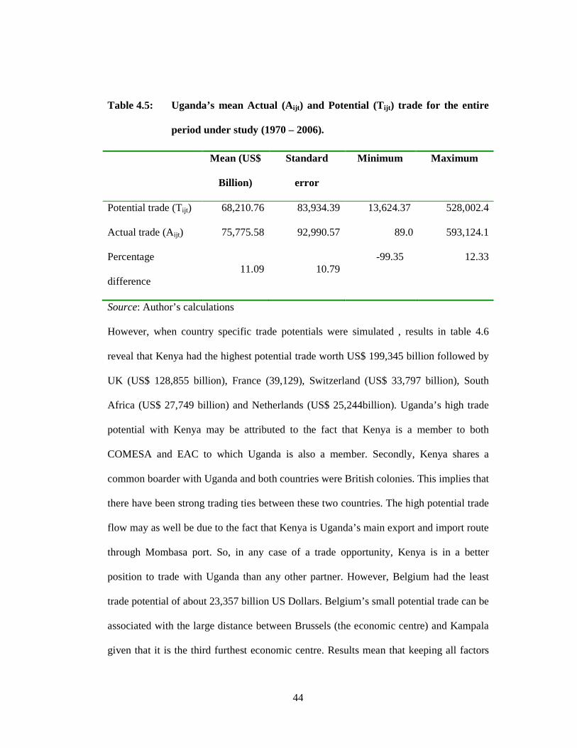
44
Table 4.5: Uganda’s mean Actual (Aijt ) and Potential (Tijt ) trade for the entire
period under study (1970 – 2006).
Mean (US$
Billion)
Standard
error
Minimum Maximum
Potential trade (Tijt) 68,210.76 83,934.39 13,624.37 528,002.4
Actual trade (Aijt) 75,775.58 92,990.57 89.0 593,124.1
Percentage
difference 11.09 10.79
-99.35 12.33
Source: Author’s calculations
However, when country specific trade potentials were simulated , results in table 4.6
reveal that Kenya had the highest potential trade worth US$ 199,345 billion followed by
UK (US$ 128,855 billion), France (39,129), Switzerland (US$ 33,797 billion), South
Africa (US$ 27,749 billion) and Netherlands (US$ 25,244billion). Uganda’s high trade
potential with Kenya may be attributed to the fact that Kenya is a member to both
COMESA and EAC to which Uganda is also a member. Secondly, Kenya shares a
common boarder with Uganda and both countries were British colonies. This implies that
there have been strong trading ties between these two countries. The high potential trade
flow may as well be due to the fact that Kenya is Uganda’s main export and import route
through Mombasa port. So, in any case of a trade opportunity, Kenya is in a better
position to trade with Uganda than any other partner. However, Belgium had the least
trade potential of about 23,357 billion US Dollars. Belgium’s small potential trade can be
associated with the large distance between Brussels (the economic centre) and Kampala
given that it is the third furthest economic centre. Results mean that keeping all factors

45
constant, Kenya, UK and France can provide a big trade base for Uganda while Belgium
has the least to offer.
Table 4.6: Uganda’s trade potential with country specific trade partners
(US$ billion)
Trade
partner
Kenya UK Switzer-
land
Nether-
lands
Belgium South
Africa
France
Potential
trade (Tijt) 199,345
128,855 33,797 25,244 23,357 27,749 39,129
Actual
trade (Aijt) 210,735
127,709 43,604 46,277 28,440 35,230 38,434
Source: Author’s calculations
According to table 4.7, the Rdijt index of 5.25 percent (0.0525) obtained between Uganda
and her trade partners indicates that Uganda has a low but good trade performance with
her trade partners over the entire 37 years’ study period. The low level of good trade
performance may be attributed to weak trade ties with her trade partners in terms of
previous economic scale and development. To a large extent, low performance can be
associated with existence of serious trade barriers between the trading partners. Such
barriers may include; Uganda being a landlocked country. Land locked-ness very much
limits trade flows with distant partners in that it leads to high transport costs, which is
one of the key determinants to successful trade. Although there are other means of
transport (Air and Railway), these can not sustain Uganda’s trade flows. For instance,
use of air transport is indeed very costly to sustain trade given that much of Uganda’s
exports are unprocessed raw materials which are bulky for this type of transport. The
alternative would then be the railway means of transport but lately, the railway network
system is not operational thereby greatly aggravating the land locked-ness issue.
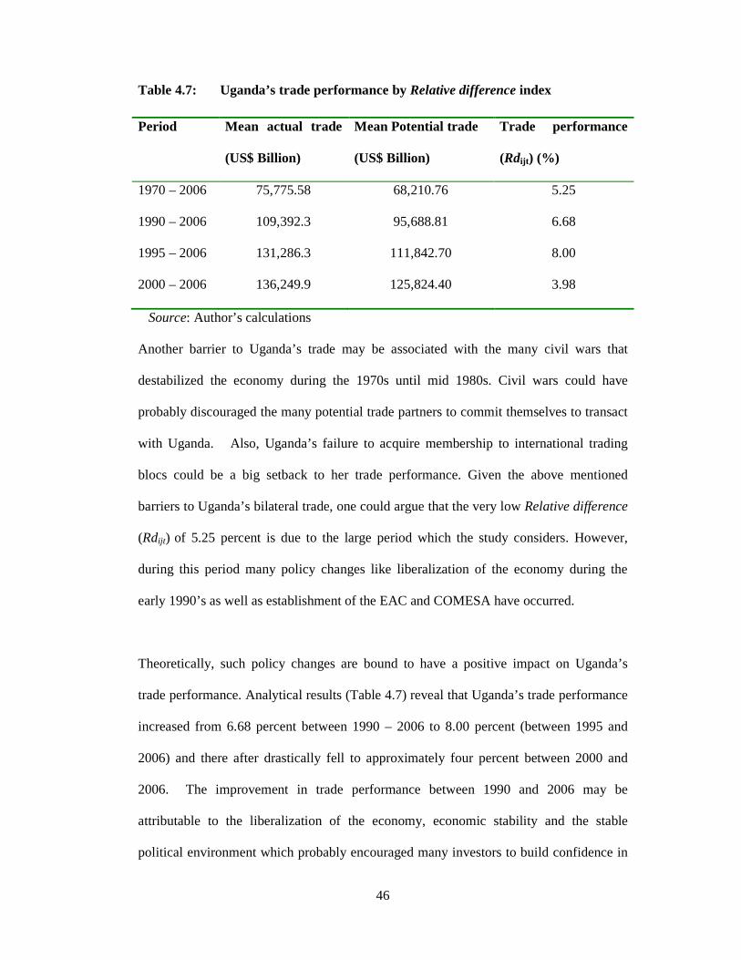
46
Table 4.7: Uganda’s trade performance by Relative difference index Period Mean actual trade
(US$ Billion)
Mean Potential trade
(US$ Billion)
Trade performance
(Rdijt ) (%)
1970 – 2006 75,775.58 68,210.76 5.25
1990 – 2006 109,392.3 95,688.81 6.68
1995 – 2006 131,286.3 111,842.70 8.00
2000 – 2006 136,249.9 125,824.40 3.98
Source: Author’s calculations
Another barrier to Uganda’s trade may be associated with the many civil wars that
destabilized the economy during the 1970s until mid 1980s. Civil wars could have
probably discouraged the many potential trade partners to commit themselves to transact
with Uganda. Also, Uganda’s failure to acquire membership to international trading
blocs could be a big setback to her trade performance. Given the above mentioned
barriers to Uganda’s bilateral trade, one could argue that the very low Relative difference
(Rdijt) of 5.25 percent is due to the large period which the study considers. However,
during this period many policy changes like liberalization of the economy during the
early 1990’s as well as establishment of the EAC and COMESA have occurred.
Theoretically, such policy changes are bound to have a positive impact on Uganda’s
trade performance. Analytical results (Table 4.7) reveal that Uganda’s trade performance
increased from 6.68 percent between 1990 – 2006 to 8.00 percent (between 1995 and
2006) and there after drastically fell to approximately four percent between 2000 and
2006. The improvement in trade performance between 1990 and 2006 may be
attributable to the liberalization of the economy, economic stability and the stable
political environment which probably encouraged many investors to build confidence in

47
the Ugandan economy. However, the decline in trade performance between 2000 and
2006 can be attributed to lack of adequate promotion of export trade, despite the fact that
bodies like the Uganda Export Promotion Board (UEPB) are trying to promote trade.
Also, much of Uganda’s trade has been focusing on only the major cash crops, that is to
say, coffee, cotton and Tobacco not knowing that there is need to diversify into other
goods and services with high market demand. For instance, UBOS (2007) puts it that
since 2005, there is a tremendous international market demand for the non traditional
cash crops like flowers, fruits and vegetables among others that Uganda could exploit but
not many firms have involved themselves in this business.
The fall in trade performance can also be attributed to the now and then changing
international market standards especially of agricultural produce where Uganda trades
most. New export standards are being made stricter so often and this limits the country’s
export trade flows especially to the international markets like the European Union among
others. For example, unlike the olden years, agricultural produce for export used not to
be subjected to so much scrutiny like it is the case now days. To date, for agricultural
produce to have good international market, it must meet Global GAP standards and
EUREPGAP standards in case one is targeting the European market. So, given that much
of Uganda’s agriculture is still at peasantry level, coupled with little or no value addition
to the produce, this has compromised on the Uganda’s involvement in agricultural trade
in international markets and so the poor trade performance. Similar results were obtained
by Chen et al. (2007) who analysed Xinjiang’s bilateral trade performance with her trade
partners and noted that Xinjiang had excellent trade cooperation notably with
Kazakhstan, Pakistan, Germany, Russia, Ukraine and France.

48
Findings of the Absolute difference index (Adijt) often referred to as unexhausted trade
potential reveal that quantitative deviations exist between Actual and Potential trade.
Approximately, over US$ 7,500 billion worth of mean unexhausted trade potential
existed between Uganda and her trade partners for the entire 37 year study period. This
volume of unexhausted trade may be associated with both natural and artificial barriers
to trade like land locked-ness, political instabilities during the 1970s, and new standards
on the international market, among others. This result is in line with findings obtained
when Rdijt index (5.25 percent) was used except that this particular index (Adijt) gives that
actual quantity by which actual trade exceeds the potential trade. Results therefore imply
that Uganda’s actual bilateral trade flow exceeded the anticipated trade potential by
about 7,500 billion US dollars. This suggests that Uganda has successful partnership
with her major trade partners. Uganda indeed traded by far more than what she ought to
have done given that the large mean unexhausted trade potential bears a positive sign.
The Adijt index was used to cross check or validate results obtained by the former index.
However, when country specific unexhausted trade potentials were analysed, results in
table 4.8 show that Uganda had been gaining from her bilateral trade flows with most of
the trade partners most especially Netherlands from whom US$ 21,033 billion was
realized followed by Kenya, Switzerland and South Africa.
49
Table 4.8: Trade performance by Absolute difference (Adijt) index by country Trade partner Unexhausted trade Potential (US$ Billion)
Kenya 11,390.5
Switzerland 9,806.8
Netherlands 21,033.3
Belgium 5,083.1
United Kingdom -1,145.6
South Africa 7,480.9
France -695.4
Overall Unexhausted trade potential 7,564.8
Source: Author’s calculations
The good trade performance may probably be attributed to the existence of good trade
terms with such countries. To be particular, although Netherlands and Switzerland are
distant from Uganda, this success story may be attributed to the fact that Uganda has
concentrated on exporting less bulky but highly valuable goods such as organically
grown fruits and vegetables among others to these countries. For example, UBOS (2007)
notes that for the past 2 – 3 years, Netherlands and Switzerland have been some of
Uganda’s major destinations of horticultural produce (Flowers, Fruits and vegetables)
and fresh fish. These commodities have earned Uganda a fortune of foreign exchange.
From the horticulture sector, Roses and cut flowers among other products contributed
about five percent of the total exports in 2003 (UBOS, 2007). So, with such successful
trading partners, it means that bilateral trade has reached its potential level. At this level,
little or no social cost should be expected from future partnerships unless when there is
more product diversification e.g. exportation of dried fruits and vegetables instead of
fresh produce.

50
On the contrary, UK and France registered large untapped trade potentials worth about
US$ 1,200 and 700 billions respectively. Uganda’s poor trade performance with UK and
France may be attributed a number of factors. Firstly, there exists large distance between
Kampala and the two economic centres, that is Paris (France) and London (UK).
Secondly, the high non tariff barriers to trade like EUREPGAP certification, Global GAP
certification and Food miles, among others put in place by such developed economies
limit Uganda’s trade to flourish on the international markets especially with agricultural
produce. In the long-run, these none tariff trade barriers limit success of the partnership,
thence causing the poor trade performance. Thirdly, it is also possibly true that there has
not been much promotion of bilateral trade flows between Uganda and these countries
(UK and France). Results signify that there is no successful partnership between Uganda
and these two countries. This is because Uganda’s actual bilateral trade flows are less
than the predicted trade potential flows. Results obtained with Absolute difference index
(Adijt) are consistent with the earlier results obtained with the relative difference index
(Rdijt). The Adijt negative value means that Uganda actually traded less than her
anticipated potential trade flow.
4.4 Uganda’s Degree of Trade integration with her trade partners
Determination of Uganda’s degree of trade integration was based on the actual trade
(A ijt) and potential trade (Tijt) for the entire 37 years on which this research focuses.
Therefore, by taking the ratio of mean actual trade to mean potential trade, Uganda’s
mean degree of trade integration was found to be 111.09 percent. This is a relatively high
ratio, implying that Uganda can easily be integrated in trade. This high degree of trade
integration can be associated with the fact that Uganda has many goods and services she
51
trades. Such goods and services include tourism attraction sites, minerals like copper and
human resource, among others. Integration can as well be due to Uganda’s inability to
process and / or manufacture a number of basic goods require by her citizens. So, in a
way to acquire these goods, she has to rely on her trading partners from whom to import
the goods. Petroleum and its products and automobiles are of late Uganda’s major
imports (UBOS, 2007).
However, considering trade integration at country level, results in table 4.9 show that all
Uganda’s trading partners have high ratios although France and the United Kingdom
have relatively lower ratios; that is, 98.22 and 99.11 percent respectively. The lower
ratios can be as a result of existence of trade barriers which limit Uganda being fully
integrated into trade with these particular countries. Such barriers include distance and
non tariff trade barriers like GLOBALPGAP certification, among others.
Table 4.9: Uganda’s degree of trade integration by country Trade partner Degree of integration (Aijt /T ijt )*100
Kenya 105.71
Switzerland 129.02
Netherlands 183.32
Belgium 121.76
United Kingdom 99.11
South Africa 126.96
France 98.22
Overall degree of trade integration 111.09
Source: Author’s calculations
52
Uganda’s low degree of trade integration into trade with UK and France can also be
attributable to the political insecurity Uganda faced during the 1970s until mid 1980s.
This probably discouraged these trade partners from build confidence and trust in
transacting with Uganda. Results strongly agree with earlier findings while using Rdijt
and Adijt trade performance indices because it is these very trade partners (UK and
France) which were identified as Uganda having had unsuccessful trade partnerships
with.
Findings further indicate that Netherlands (183.32), Switzerland (129.02), South Africa
(126.96) and Belgium (121.76) have very high ratios, implying that Uganda has a high
degree of trade integration with these trade partners. The high degree of trade integration
can be attributed to the good cooperation between the trade partners. For instance,
Uganda’s high degree of trade integration with South Africa can be due to fact that both
countries are members to COMESA, therefore compelling both parties to be in good
trading terms following the signed Memorandum of understanding agreed upon at the
inception of COMESA as a trade bloc. However, for the other countries (Netherlands,
Switzerland and Belgium), the high degree of integration may be attributed to Uganda’s
being one of the few countries that can supply organically grown foodstuff and this
renders her as an inevitable stakeholder in trade especially for the supply of horticultural
products.
Results obtained by measuring Uganda’s degree of trade integration based on the dummy
variables (Table 4.10) indicate that having had similar colonial masters (DUK) has the
highest trade integration effect (351.99) on Uganda’s bilateral trade flows. The high
integration effect can be attributed to the trade agreements that the colonial masters put

53
in place so as to foster trade collaboration among her territories. For instance, on behalf
of Uganda, Britain had to ensure that Kenya (also once a British colony) granted Uganda
access to the Western world through Mombasa Port which to date is the mostly used port
for trade. Findings mean that Uganda’s bilateral trade flow between partners once
colonised by Britain is 352 percent as great as that with partners that were not British
colonies. This is probably one of the reasons why Kenya is one of Uganda’s leading
trade partners.
Table 4.10: Uganda’s degree of trade integration based on COMESA and EAC
on dummy variables
Dummy
Variable
FGLS
Coefficient
Standard error [(exp(dummy coefficient)-1)] *
100
DCOMESA 0.8339** 0.3304 130.23
DEAC 0.0019 0.3086 0.19
DUK 1.5085*** 0.1367 351.99
*** and ** Denotes significant at 1% and 5 % level respectively
Source: Author’s calculations
Membership to COMESA (DCOMESA) also registered integration effects on Uganda’s
bilateral trade flows more than membership to the EAC (DEAC). Uganda’s bilateral
trade flows between COMESA member countries is 130.23percent more than bilateral
trade flows between otherwise COMESA member countries. This effectiveness of
membership to COMESA in boosting Uganda’s bilateral trade can be as a result of the
many countries in this trading bloc than they are in the East African Community. Results
indicate that membership to EAC (DEAC) does not significantly influence Uganda’s
bilateral trade flow. Membership to EAC has the least degree of trade integration of 0.19
54
as compared to common colonial master and COMESA membership dummy results. The
least degree of trade integration can be attributed to the fact that East Africa regional
bloc has not been in existence as an FTA for long to count so much on Uganda’s trade
flows. Also, this region does not have many countries and of the few there are, much of
the trade is with Kenya. CPD (2006) and Sandra (2006) obtained comparable results.

55
CHAPTER FIVE
SUMMARY, CONCLUSIONS AND RECOMMENDATIONS
5.1 Summary
The study aimed at determining factors affecting Uganda’s total bilateral trade flows and
her trade Potential. Specifically, the study predicted Uganda’s bilateral trade flows and
performance. The study also determined Uganda’s degree of trade integration with her
major trade partners. Descriptive statistics including means and standard deviations were
computed using STATA software. The descriptive statistics were used to examine the
socio-economic characteristics of Uganda and her various trade partners. Results showed
that Uganda’s average total bilateral trade was US$ 76 million while her average real
GDP was valued at 4.52 billion US Dollars. The average real GDP of the trading
partners was US$ 426.15 billion; mean population was at 17.5 and 29.1 million people
for Uganda and her trading partners respectively. Average distance between Kampala
and any other capital city of the trading partners was 3,052 mile.
It was hypothesized that there are various factors that determine total bilateral flows
between Uganda and her major trade partners. An Augmented-gravity flow model was
estimated using the Feasible Generalised Least Squares (FGLS) estimator to determine
those factors that affect total bilateral flows. Estimates of this function showed that real
GDPs, membership to COMESA, common colonial masters and membership to the East
African Community (EAC) positively influenced Uganda’s bilateral trade flows.
Population of both Uganda and her trading partners, distance, real exchange rate
volatility, and real exchange rate misalignment however indicated that they negatively
influence bilateral trade flows. Overall, the hypotheses that Uganda’s real GDP and real
56
GDP of her trading partners positively influence bilateral trade flows; and that the longer
the distance from Kampala city to the capital city of a major trade partner would lower
the level of bilateral trade flow were not rejected. Similarly, real exchange rate volatility
and real exchange rate misalignment were found to negatively influence Uganda’s
bilateral trade flows as hypothesised.
In predicting Uganda’s bilateral trade potential, an out of sample approach was employed
and the simulated trade flows were used to analyse trade performance using two indices,
that is, Relative difference (Rdijt) and Absolute difference (Adijt). Uganda’s mean potential
trade was estimated at US$ 68,211billion with Kenya as the major trade partner followed
by the United Kingdom. However, Belgium and Netherlands registered the lowest trade
potentials estimated at US$ 23,357 and US$ 25,244 respectively. Trade performance
results from the Rdijt index revealed that Uganda had good trade performance estimated
at 5.25 percent over the entire study period (1970 – 2006). Analytical results of post
economic liberalization revealed that trade performance improved gradually from 6.68
percent between 1990 and 2006 to 8.00 percent between1995 to 2006 and then
drastically dropped to about 4.0 percent (3.98 %) between 2000 and 2006. Results from
the Absolute difference (Adijt) index showed that Uganda benefited from her bilateral
trade by about US$ 7,972 billion, implying good trade performance.
In addition, a ratio of actual to potential bilateral trade flow was estimated to
generate Uganda’s degree of trade integration. Results revealed that Uganda had a
high degree of trade integration (111.09 percent) with all her trading partners. However,
at country level, Uganda cannot easily integrate with UK and France given the lower
ratios of 0.99 and 0.98 respectively. Analysis of Uganda’s degree of trade integration
57
measured basing on dummy variables showed that Uganda had a higher degree of trade
integration with trade partners belonging to COMESA unlike with non-COMESA trade
partners. Uganda’s trade with COMESA countries was 130% as much as that with non-
COMESA partners. A low degree of trade integration (0.19 %) was observed among
EAC partners unlike among non-EAC partners.

58
5.2 Conclusions
Several conclusions can be drawn from this study. Uganda’s real GDP, real GDP of her
trade partners, trade partners’ real GDP, distance between Uganda (Kampala) and the
capital city of her trading partner, trading partners’ population, real exchange rate
volatility, real exchange rate misalignment, membership to COMESA and colonial ties
have been found to be significant determinants of Uganda’s bilateral trade flows.
Therefore, any efforts to improve Uganda’s bilateral trade flows should focus on
activities like proper real exchange rate management. Uganda’s GDP, colonial ties to
Britain and membership to COMESA have the most influential effect on her bilateral
trade flows.
Uganda has low but good trade performance. Thus, there are some barriers to trade that
are still hindering the growth of bilateral trade flows in Uganda. Uganda had successful
trade partnerships with Belgium, Netherlands, Kenya, Switzerland and South Africa.
More fostering in trade cooperation between France and UK is still desirable to improve
Uganda’s trade integration with these economies. All in all, Uganda can easily be trade
integrated with all her trade partners although not so easily with France and UK.
Netherlands, Switzerland, South Africa and Kenya have good cooperation with Uganda
in terms of trade.
5.3 Recommendations
It is recommended that policy makers should consider strengthening the EAC trade
agreements and those with COMESA member countries as shown by the determinants of
Uganda’s bilateral trade flows. This will greatly reduce on the many non-tariff trade
barriers that Uganda encounters in her bilateral trade and broaden her trading network.

59
Policies to minimize real exchange volatility and misalignment should be strengthened to
improve trade flows.
To improve Uganda’s trade performance with France and the UK, it is desirable for
Ministry of Tourism and Trade together with government bodies like the Uganda Export
Promotion Board (UEPB) to promote trade partnerships with such countries at
government level rather than at private level. The government should also advocate and
lobby for revisiting some the international market standards like GLOBALGAP
certification requirements which have made Uganda retard in trade. However, given that
it may not be feasible for a small economy like Uganda to influence the changing of such
internationally set standards, the private and public sectors may team up and establish
national GAP standards. This will then act as a benchmark to attain the international
standards in the long-run.
Alternatively, Uganda should also think of diversification of her products so as to expand
her bilateral trade flows. Diversification may for example be taken in form of value
addition to agro-produce since this is one of Uganda’s major exports. Value addition
increases the shelf life of produce and reduces bulkiness of produce. Uganda should also
put in place strategies and policies that can reduce the many trade barriers. For example,
government should invest generously in public infrastructure like roads to link Uganda to
major ports in Africa. The Ugandan government should subsidise freight costs in the
interest of exporters since this is the surest and fastest means to deliver perishable
agriculture produce to international markets.
60
5.3 Areas for further research
While this study attempted to ascertain determinants of Uganda’s bilateral trade flows
with her major trade partners since 1970 up to 2006, data employed was not
disaggregated at sector level. Data was generally aggregated as exports and imports to
and from trading partners. However, total bilateral trade can be decomposed on sector
basis, that is, total agricultural imports and exports, total manufactured imports and
exports or total livestock product imports and exports. Therefore, further research using
disaggregated data at sector level is necessary to distinguish and identify the specific
determinants of bilateral trade at sector level.
REFERENCES
Achay L. (2006). Assessing Regional Integration in North Africa,’ National Institute of Statistics and Applied economics, Rabat, Morocco.
Amita, B. (2004). India’s global trade potential: The gravity model approach. New Dheli, India.
Indian Council for Research on International Economic Relations.
Anderson, J.H. (1979). “A Theoretical Foundation for the Gravity Equation”. American Economic Review, 69: 106 – 116.
Baldwin, R.E. (1994). Towards an Integrated Europe. CEPR. Graduate Institute of
International Studies, Ave de la Pais, 1202 Geneva. Bergstrand, J. H. (1989). 'Trade generalized gravity equation, monopolistic competition, and the
factor-proportions theory in international trade', Review of Economics and Statistics, 71:143 – 153.
______ (1985). “The Gravity Equation in International Trade: Some Microeconomic
Foundations and Empirical Evidence”. Review of Economics and Statistics, 67: 474 – 481.

61
Bougheas, S., Demetriades, P.O. and Morgenroth E. L. W. (1999). “Infrastructure, Transport Costs and Trade,” Journal of International Economics, 47:169 – 189.
Brulhart M. and Kelly M.J. (1999). Ireland's trading potential with central and eastern
European countries: A gravity study. Economic and Social Review, 30(2): 159 – 174.
Buch, C. M., Kleinert, J. and Toubal F. (2003). The Distance puzzle: On the interpretation of the distance coefficient in the Gravity equations, Kiel Working Paper No. 1159.
Chan-Hyun S. (2005). Does the gravity model explain South Korea’s trade flows? The
Japanese Economic Review, 56(4): 417 - 430. Chen, X., Yang, Z. and Lui, X. (2007). Empirical Analysis of Xinjiang’s Bilateral Trade:
Gravity Model Approach. Chinese Geographical Science, 18(1): 9 -16. Available at www.springer/link.com
Cho, G., Sheldon, I. and McCorriston, S. (2002).Exchange Rate Uncertainity and Agricultural Trade. American Journal of Agricultural Economics 84:934 – 942.
Cote, A. (1994). Exchange rate volatility and trade. Working Paper 94-5 / Document de travail
94-5. CPD (2006). Trade Potential in SAFTA: An Application of Augmented Gravity Model. ISSN
1818 – 1570 (Print). ISSN 1818 – 1597 (Online). Deardorff, A. V., (1998). Determinants of bilateral trade: Does gravity work in a neoclassical
world? The Regionalization of the World Economy, pp. 7–28. University of Chicago Press, Chicago.
De Grauwe, P. (1988). Exchange Rate Volatility and the Slowdown in Growth of International
Trade. IMF Staff Papers 24: 317 – 330. De Sousa, J. and Disdier, A., (2002). “Trade, Border Effects and Individual Characteristics: A
Proper Specification,” unpublished Manuscript, University of Paris 1. Egger, P., (2000). A note on the proper econometric specification of the gravity equation.
Economics Letters, 66: 25-31. Eichengreen, B., and Irwin, D. (1995). Trade Blocs, Currency Blocs and the Reorientation of
Trade in the 1930s. Journal of International Economics 38:1 – 24. Eichengrean, B., and Irwin, D., (1997). The role of history in bilateral trade flows: The
Regionalisation of the World Economy, Frankel J., ed., University of Chicago Press, 33 – 57.
EPAU, (1995). Exporters’ Survey 1995: Impact of government policy on exports a focus on
NTAEs, Kampala: Export Policy Analysis Unit, Ministry of Finance and Economic Planning.

62
Feenstra, R. C., Markusen, J.R. and Rose A.K. (2001). Using the Gravity Equation to Differentiate among Alternative Theories of Trade. Canadian Journal of Economics, 34: 430-447.
Foldvari, P., (2000). The Economic Impact of the European Integration on Netherlands. A
quantitative analysis of Foreign trade and foreign direct investments. Pp.1- 143 Universiteit Utrecht. Available on http://igitur-archive.library.uu.nl
Frankel, J., and Wei, S. (1993). Trade Blocs and Currency Blocs. NBER Working Paper No.
4335. Frankel, J., (1997). Regional Trading Blocs in the World Trading System. Washington, DC:
Institute for International Economics, xv, 364: ISBN 0881322024. Gardner, B. (1981). On the Power of Macroeconomic Linkages to Explain Events in U.S.
Agriculture. American Journal of Agricultural Economics 63: 872-878. Geda, A., (2002). Regional Economic Integration in Africa: A review of Problems and
Prospects with a case study of COMESA. Journal of African Economies, 17(3): 357 – 394.
Giorgio, R., (2004). Empirical Evidence on the North-South Trade Flows: An Augmented Gravity Model. MPRA Paper No. 136. Available at http://mpra.ub.uni-muenchen.de.
Grossman, G. (1998). Determinants of Bilateral Trade: Does Gravity Work in a Neoclassical
World? The Regionalization of the World Economy, Jeffrey A. Frankel ed. Cambridge, MA: National Bureau of Economic Research. pp. 29-31.
Gue, D. C., MinKyoung, K., Edwin, S., Hyun, J., and Won, W. K. (2003). Nominal Exchange
Rate Misalignment: Is It Particularly Important to Agricultural Trade? Agribusiness & Applied Economics Report No. 516 August 2003
Hamilton, C.B., and Winters, A. L., (1992). Opening Up International Trade with Eastern
Europe. Economic Policy, 14: 77 – 116.
Helmers, C. and Pasteals J.M. (2003). A gravity model for the calculation of trade potentials for developing countries and economies in transition. Geneva, Switzerland: International Trade Centre.
IMF (2007). International Financial Statistics Yearbook. International Monetary Fund.
Statistics Department. ISSN: 0250-7463. ______ (1998). International Financial Statistics Yearbook. International Monetary Fund.
Statistics Department. ISSN: 0234-7621. Inmaculada, M. Z. and Felicitas, N. L.D., (1998). Augmented gravity model: An empirical
application to Mercosur-European trade flows. DB Nr. 77. ITC, (2003). TradeSim. A Gravity Model for the calculation of Trade Potentials for Developing
Countries and economies in transition, Technical report, UNCTAD – WTO.
63
Jiang, D., (2003). Study on the interaction between NDVI profile and the growing status of crops. Chinese Geographical Science, 13(1): 62 – 65.
Kalbasi, H., (2004). The gravity model and global trade flows. University of Isfahan,
Department of Economics. Kandilov, I. T. (2008). The Effects of Exchange rate Volatility on Agricultural Trade. American
Journal of Agricultural Economics 90: 1028 – 1043. Keith, H., (2003). Gravity for beginners. Faculty of Commerce, University of British Columbia,
Canada. At available at www.economics.ca/keith/gravity.pdf Klein, M. (1990). Sectoral Effects of Exchange Rate Volatility on United States Exports.
Journal of International Money and Finance 9: 299 – 308. Li, L., Liu Z. and Li C. (2002). Spatial correlation analysis of crop yield in the middle and West
of Jilin Province. Chinese Geographical Science, 12(2): 182 – 185. Lin, L., and Wang Y., (2004). Empirical test of China’s bilateral trade with the trade gravity
model and its policy implications. World Economy Study, 7: 56 – 60. Liu, Q., and Jiang, S., (2002). Study on the Chinese bilateral trade arrangement using the
gravity model. Zhejiang Social Sciences, 6: 17 – 20. Luca, D. B., and Vicarelli, C., (2004). Trade potential in gravity Panel Data models. The B. E.
Journal of Economic Analysis and Policy, 5(1) Article 20. Available at http:// www.bepree.com/bejeap
Martinez-Zarzoso, I., (2003). Augmented Gravity Model: An empirical application to
Mercosur-European Union trade flows. Journal of Applied Economics, 6(2):291 – 316.
Morrissey, O., and Rudaheranwa, N., (1998). Ugandan trade policy and export performance in
the 1990s. Credit discussion paper 6 (CDP006). No. 98/12. Muhammad, A. and Andrews, D., (2008). Determining tourist arrivals in Uganda: The impact
of distance, trade and origin: Specific factors. African Journal of Accounting, Economics, Finance and Banking Research, 2(2): 51-62.
Nilsson, L., (2000). Trade Integration and the EU Economic Membership Criteria. European
Journal of Political Economy, 85: 615 – 623. Sandra, P., (2006). Economic Integration of Yunnan with the Great Mekong Sub-region. Asian
Economic Journal, 20(3): 303–317. Scollay, R., and Gilbert, J., (2001): New regional trading arrangements in the Asia Pacific,
Washington, DC: Institute for International Economics. Sheng, B. and Liao, M., (2004). China’s trade flows and export potential: The gravity model
approach. World Economy, 27(2): 4 – 10.

64
Sokchea K., (2006). An analysis of Cambodia’s Trade Flows: A Gravity Model. Working Paper Series, pp. 1 – 24. Available at www.papers.ssrn.com
Thursby, J., and Thursby, M. (1987). Bilateral Trade Flows, the Linder Hypothesis and
Exchange Rate Risk. Review of Economics and Statistics 82: 485 – 508. Tweeten, L. (1989). Farm Policy Analysis. Westview Press, 1989. UBOS, (2007): Statistical Abstract. Uganda Bureau of Statistics, Kampala, Uganda. UBOS, (2006): Statistical Abstract. Uganda Bureau of Statistics, Kampala, Uganda. UNCTAD, (1999). UNCTAD's contribution to the implementation of the United Nations new
agenda for the development of Africa in the 1990s: African transport infrastructure, trade and competitiveness, Technical report, UNCTAD Secretariat. TD/B/46/10. Online at: http://www.unctad.org/en/docs/tb21d2.pdf
Wang, Z., and Winters, A.L., (1992). The Trading Potential of Eastern Europe, Journal of
Economic Integration, 7: 113 - 136.
Whalley, J., (1998). Why do countries seek regional trade agreements? In: Frankel J.A (ed.): The regionalization of the world Economy. Chicago. University of Chicago Press, 63 – 82.
Wall, J., H., (1999). Using the Gravity model to estimate the costs of Protection. January/
February Review of Federal Bank of Saint Louis.

65
Appendix A: FGLS estimation output
. xtgls lnbtrade lnug_gdp lnoth_gd lnug_pop lnoth_po lndist lnvol misalign dcomesa deac duk, panels (hetero) Cross-sectional time-series FGLS regression Coefficients: generalized least squares Panels: heteroskedastic Correlation: no autocorrelation Estimated covariances = 7 Number of obs = 259 Estimated autocorrelations = 0 Number of groups = 7 Estimated coefficients = 11 Time periods = 37
Wald chi2(10) = 659.63 Log likelihood = -262.2464 Prob > chi2 = 0.0000 lnbtrade Coef. Std. Err. z P>z [95% Conf. Interval] lnug_gdp 0.7357034 0.2283482 3.22 0.001 .2881491 1.183258 lnoth_gd 0.6426558 0.1633435 3.93 0.000 .3225083 .9628033 lnug_pop - 0.6034084 0.3231401 -1.87 0.062 -1.236751 .0299345 lnoth_po - 0.4431255 0.1633296 -2.71 0.007 -.7632457 -.1230053 lndist - 1.439406 0.1926796 -7.47 0.000 -1.817051 -1.061761 lnvol - 0.0709397 0.0246821 -2.87 0.004 -.1193157 -.0225636 misalign - 0.0033926 0.001419 -2.39 0.017 -.0061737 -.0006114 dcomesa 0.8339322 0.3303846 2.52 0.012 .1863903 1.481474 deac 0.001913 0.3086394 0.01 0.995 -.6030092 .6068351 duk 1.508453 0.1366942 11.04 0.000 1.240537 1.776368 _cons 20.91197 1.499226 13.95 0.000 17.97355 23.8504
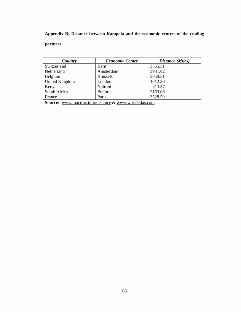
66
Appendix B: Distance between Kampala and the economic centres of the trading
partners
Country Economic Centre Distance (Miles)
Switzerland Bern 3555.51 Netherland Amsterdam 3931.82 Belgium Brussels 3859.31 United Kingdom London 4012.36 Kenya Nairobi 313.57 South Africa Pretoria 2163.06 France Paris 3528.59 Source: www.macrow.info/distance & www.worldatlas.com
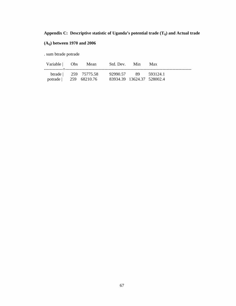
67
Appendix C: Descriptive statistic of Uganda’s potential trade (T ij ) and Actual trade
(A ij ) between 1970 and 2006
. sum btrade potrade Variable | Obs Mean Std. Dev. Min Max -------------+--------------------------------------------------------------------------------------- btrade | 259 75775.58 92990.57 89 593124.1 potrade | 259 68210.76 83934.39 13624.37 528002.4
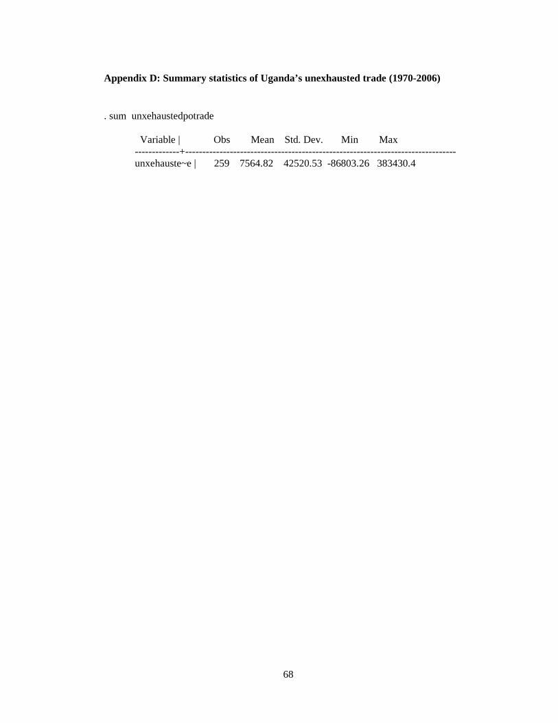
68
Appendix D: Summary statistics of Uganda’s unexhausted trade (1970-2006)
. sum unxehaustedpotrade Variable | Obs Mean Std. Dev. Min Max
-------------+------------------------------------------------------------------------------- unxehauste~e | 259 7564.82 42520.53 -86803.26 383430.4
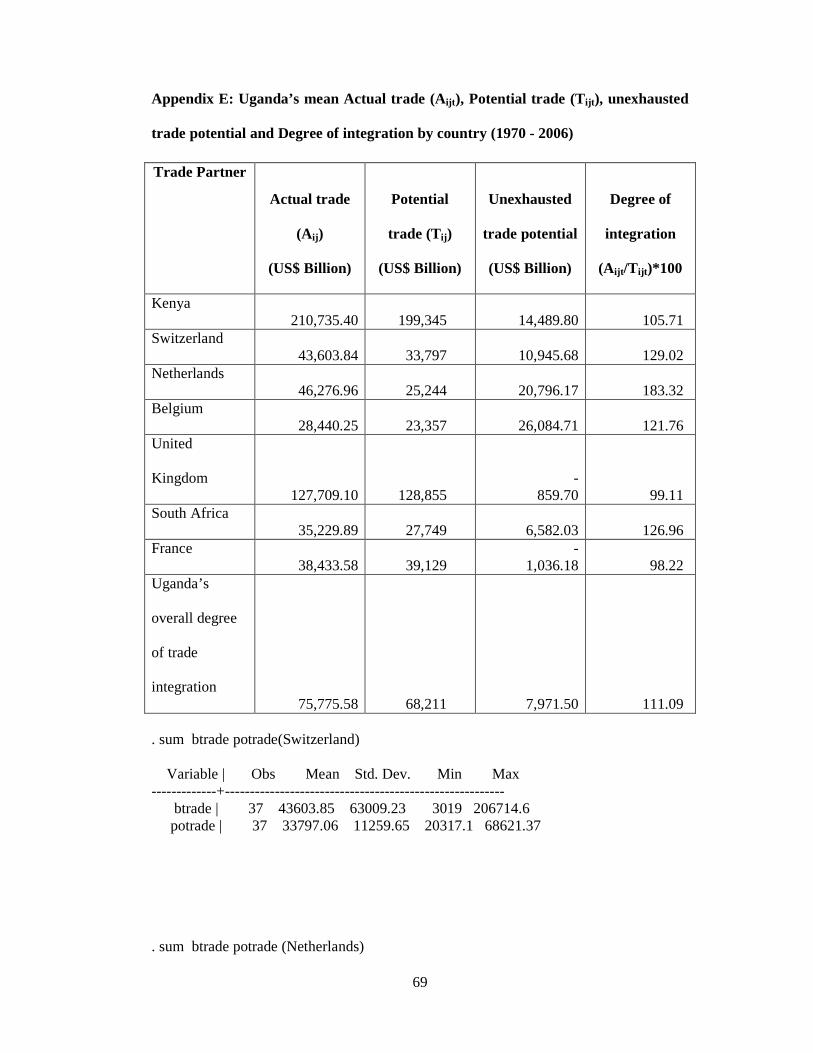
69
Appendix E: Uganda’s mean Actual trade (Aijt ), Potential trade (Tijt ), unexhausted
trade potential and Degree of integration by country (1970 - 2006)
Trade Partner
Actual trade
(A ij )
(US$ Billion)
Potential
trade (Tij )
(US$ Billion)
Unexhausted
trade potential
(US$ Billion)
Degree of
integration
(A ijt /T ijt )*100
Kenya 210,735.40 199,345
14,489.80 105.71
Switzerland 43,603.84 33,797
10,945.68 129.02
Netherlands 46,276.96 25,244
20,796.17 183.32
Belgium 28,440.25 23,357
26,084.71 121.76
United
Kingdom 127,709.10 128,855
-859.70 99.11
South Africa 35,229.89 27,749
6,582.03 126.96
France 38,433.58 39,129
-1,036.18 98.22
Uganda’s
overall degree
of trade
integration 75,775.58 68,211
7,971.50 111.09
. sum btrade potrade(Switzerland) Variable | Obs Mean Std. Dev. Min Max -------------+-------------------------------------------------------- btrade | 37 43603.85 63009.23 3019 206714.6 potrade | 37 33797.06 11259.65 20317.1 68621.37 . sum btrade potrade (Netherlands)
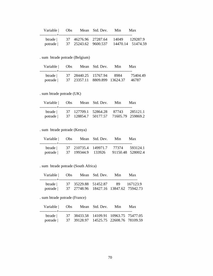
70
Variable | Obs Mean Std. Dev. Min Max -------------+-------------------------------------------------------- btrade | 37 46276.96 27287.64 14049 129287.9 potrade | 37 25243.62 9600.537 14470.14 51474.59 . sum btrade potrade (Belgium) Variable | Obs Mean Std. Dev. Min Max -------------+-------------------------------------------------------- btrade | 37 28440.25 15767.94 8984 75404.49 potrade | 37 23357.11 8809.899 13624.37 46787 . sum btrade potrade (UK) Variable | Obs Mean Std. Dev. Min Max -------------+-------------------------------------------------------- btrade | 37 127709.1 52864.28 87743 285121.1 potrade | 37 128854.7 50177.57 71605.79 259869.2 . sum btrade potrade (Kenya) Variable | Obs Mean Std. Dev. Min Max -------------+-------------------------------------------------------- btrade | 37 210735.4 149971.7 77374 593124.1 potrade | 37 199344.9 133926 91150.48 528002.4 . sum btrade potrade (South Africa) Variable | Obs Mean Std. Dev. Min Max -------------+------------------------------------------------------------ btrade | 37 35229.88 51452.87 89 167123.9 potrade | 37 27748.96 18427.16 13847.62 75942.73 . sum btrade potrade (France) Variable | Obs Mean Std. Dev. Min Max -------------+-------------------------------------------------------- btrade | 37 38433.58 14109.91 10963.75 75477.05 potrade | 37 39128.97 14525.75 22608.76 78109.59
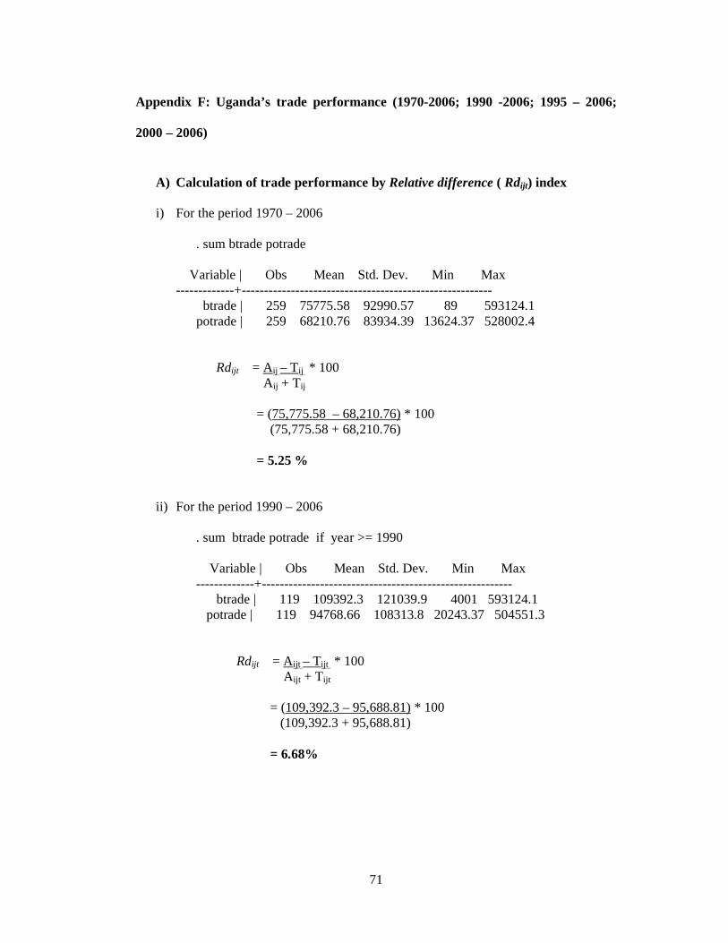
71
Appendix F: Uganda’s trade performance (1970-2006; 1990 -2006; 1995 – 2006;
2000 – 2006)
A) Calculation of trade performance by Relative difference ( Rdijt) index
i) For the period 1970 – 2006
. sum btrade potrade
Variable | Obs Mean Std. Dev. Min Max -------------+--------------------------------------------------------
btrade | 259 75775.58 92990.57 89 593124.1 potrade | 259 68210.76 83934.39 13624.37 528002.4
Rdijt = Aij – Tij * 100 Aij + Tij
= (75,775.58 – 68,210.76) * 100
(75,775.58 + 68,210.76)
= 5.25 %
ii) For the period 1990 – 2006
. sum btrade potrade if year >= 1990 Variable | Obs Mean Std. Dev. Min Max -------------+-------------------------------------------------------- btrade | 119 109392.3 121039.9 4001 593124.1 potrade | 119 94768.66 108313.8 20243.37 504551.3
Rdijt = Aijt – Tijt * 100 Aijt + Tijt
= (109,392.3 – 95,688.81) * 100 (109,392.3 + 95,688.81)
= 6.68%
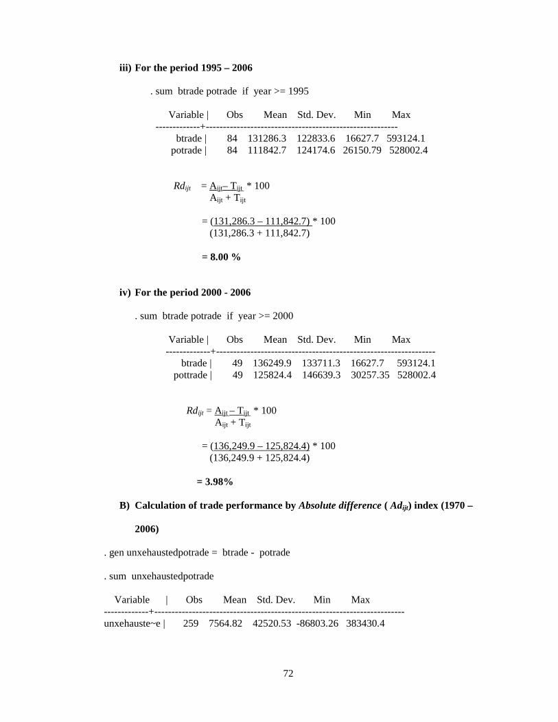
72
iii) For the period 1995 – 2006
. sum btrade potrade if year >= 1995
Variable | Obs Mean Std. Dev. Min Max -------------+--------------------------------------------------------
btrade | 84 131286.3 122833.6 16627.7 593124.1 potrade | 84 111842.7 124174.6 26150.79 528002.4
Rdijt = Aijt– Tijt * 100 Aijt + Tijt
= (131,286.3 – 111,842.7) * 100 (131,286.3 + 111,842.7) = 8.00 %
iv) For the period 2000 - 2006
. sum btrade potrade if year >= 2000 Variable | Obs Mean Std. Dev. Min Max
-------------+---------------------------------------------------------------- btrade | 49 136249.9 133711.3 16627.7 593124.1 pottrade | 49 125824.4 146639.3 30257.35 528002.4
Rdijt = Aijt – Tijt * 100 Aijt + Tijt
= (136,249.9 – 125,824.4) * 100 (136,249.9 + 125,824.4)
= 3.98%
B) Calculation of trade performance by Absolute difference ( Adijt) index (1970 –
2006)
. gen unxehaustedpotrade = btrade - potrade . sum unxehaustedpotrade Variable | Obs Mean Std. Dev. Min Max -------------+------------------------------------------------------------------------- unxehauste~e | 259 7564.82 42520.53 -86803.26 383430.4
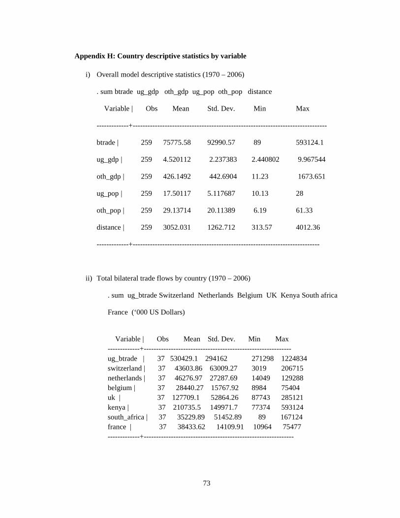
73
Appendix H: Country descriptive statistics by variable
i) Overall model descriptive statistics (1970 – 2006)
. sum btrade ug_gdp oth_gdp ug_pop oth_pop distance
Variable | Obs Mean Std. Dev. Min Max
-------------+-------------------------------------------------------------------------------
btrade | 259 75775.58 92990.57 89 593124.1
ug_gdp | 259 4.520112 2.237383 2.440802 9.967544
oth_gdp | 259 426.1492 442.6904 11.23 1673.651
ug_pop | 259 17.50117 5.117687 10.13 28
oth_pop | 259 29.13714 20.11389 6.19 61.33
distance | 259 3052.031 1262.712 313.57 4012.36
-------------+----------------------------------------------------------------------------
ii) Total bilateral trade flows by country (1970 – 2006)
. sum ug_btrade Switzerland Netherlands Belgium UK Kenya South africa
France (‘000 US Dollars)
Variable | Obs Mean Std. Dev. Min Max -------------+------------------------------------------------------------ ug_btrade | 37 530429.1 294162 271298 1224834 switzerland | 37 43603.86 63009.27 3019 206715 netherlands | 37 46276.97 27287.69 14049 129288 belgium | 37 28440.27 15767.92 8984 75404 uk | 37 127709.1 52864.26 87743 285121 kenya | 37 210735.5 149971.7 77374 593124 south_africa | 37 35229.89 51452.89 89 167124 france | 37 38433.62 14109.91 10964 75477 -------------+-------------------------------------------------------------
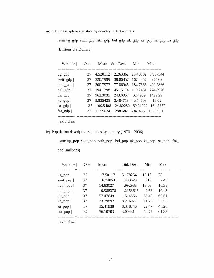
74
iii) GDP descriptive statistics by country (1970 – 2006)
.sum ug_gdp swit_gdp neth_gdp bel_gdp uk_gdp ke_gdp sa_gdp fra_gdp
(Billions US Dollars)
Variable | Obs Mean Std. Dev. Min Max -------------+---------------------------------------------------------------- ug_gdp | 37 4.520112 2.263862 2.440802 9.967544 swit_gdp | 37 220.7999 38.06857 167.4857 275.02 neth_gdp | 37 300.7973 77.86945 184.7666 429.2866 bel_gdp | 37 194.1298 45.15174 119.2451 274.8976 uk_gdp | 37 962.3035 243.0057 627.989 1429.29 ke_gdp | 37 9.835425 3.484718 4.374603 16.02 sa_gdp | 37 109.5408 24.80282 69.21922 164.2877 fra_gdp | 37 1172.074 288.682 694.9222 1673.651 -------------+---------------------------------------------------------------- . exit, clear
iv) Population descriptive statistics by country (1970 – 2006)
. sum ug_pop swit_pop neth_pop bel_pop uk_pop ke_pop sa_pop fra_
pop (millions)
Variable | Obs Mean Std. Dev. Min Max -------------+------------------------------------------------------------------------------ ug_pop | 37 17.50117 5.178254 10.13 28 swit_pop | 37 6.740541 .403629 6.19 7.45 neth_pop | 37 14.83027 .992988 13.03 16.38 bel_pop | 37 9.988378 .2153616 9.66 10.43 uk_pop | 37 57.47649 1.514556 55.42 60.51 ke_pop | 37 23.39892 8.216977 11.23 36.55 sa_pop | 37 35.41838 8.318746 22.47 48.28 fra_pop | 37 56.10703 3.004314 50.77 61.33 -------------+----------------------------------------------------------------------------- . exit, clear
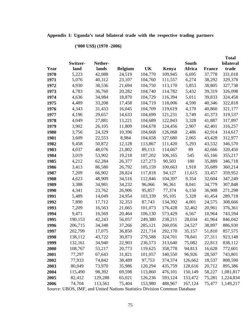
75
Appendix I: Uganda’s total bilateral trade with the respective trading partners
(‘000 US$) (1970 -2006)
Year Switzer-
land Nether-lands Belgium UK Kenya
South Africa France
Total bilateral
trade 1970 5,223 42,088 24,519 104,770 109,945 6,695 37,778 331,018 1971 5,076 40,312 23,107 104,760 111,557 6,274 38,292 329,378 1972 4,930 38,536 21,694 104,750 113,170 5,853 38,805 327,738 1973 4,783 36,760 20,282 104,740 114,782 5,432 39,319 326,098 1974 4,636 34,984 18,870 104,729 116,394 5,011 39,833 324,458 1975 4,489 33,208 17,458 104,719 118,006 4,590 40,346 322,818 1976 4,343 31,433 16,045 104,709 119,619 4,170 40,860 321,177 1977 4,196 29,657 14,633 104,699 121,231 3,749 41,373 319,537 1978 4,049 27,881 13,221 104,689 122,843 3,328 41,887 317,897 1979 3,902 26,105 11,809 104,678 124,456 2,907 42,401 316,257 1980 3,756 24,329 10,396 104,668 126,068 2,486 42,914 314,617 1981 3,609 22,553 8,984 104,658 127,680 2,065 43,428 312,977 1982 9,458 50,872 12,128 113,867 111,420 5,293 43,532 346,570 1983 4,037 48,076 21,802 89,113 114,667 89 42,666 320,450 1984 3,019 53,902 19,218 107,202 106,165 545 65,166 355,217 1985 4,212 62,284 26,377 127,273 90,503 180 35,889 346,718 1986 3,413 86,580 26,792 105,159 100,663 1,918 35,689 360,214 1987 7,209 66,902 28,824 117,818 94,127 11,615 33,457 359,952 1988 4,623 48,909 34,516 112,846 104,397 9,354 32,604 347,249 1989 3,388 34,981 34,232 96,066 96,361 8,041 34,779 307,848 1990 4,341 23,762 26,906 95,857 77,374 6,150 36,908 271,298 1991 5,489 14,049 24,954 103,339 95,105 5,328 41,454 289,718 1992 7,890 17,712 32,353 87,743 134,392 4,001 24,575 308,666 1993 7,209 16,563 21,665 101,073 176,428 32,462 20,961 376,361 1994 9,471 16,569 20,464 106,130 573,429 6,567 10,964 743,594 1995 190,153 42,243 56,057 249,380 238,211 28,034 41,964 846,042 1996 206,715 34,348 37,266 285,121 260,056 24,527 38,897 886,930 1997 202,799 17,075 36,850 221,714 292,170 35,157 51,810 857,575 1998 138,112 43,722 30,873 279,588 324,701 78,841 27,311 923,148 1999 132,161 34,940 22,903 236,573 313,640 75,082 22,813 838,112 2000 108,767 53,217 20,773 119,625 358,778 94,813 16,628 772,601 2001 77,297 67,643 31,821 101,057 340,550 96,926 28,507 743,801 2002 77,933 74,842 38,489 97,753 374,374 126,662 18,537 808,590 2003 80,049 73,970 35,986 120,294 435,759 128,616 20,712 895,386 2004 115,490 98,392 69,598 113,860 476,101 150,149 58,227 1,081,8172005 82,412 129,288 65,021 126,236 593,124 153,472 75,281 1,224,8342006 74,704 113,561 75,404 153,980 488,967 167,124 75,477 1,149,217Source: UBOS, IMF, and United Nations Statistics Division Common Database
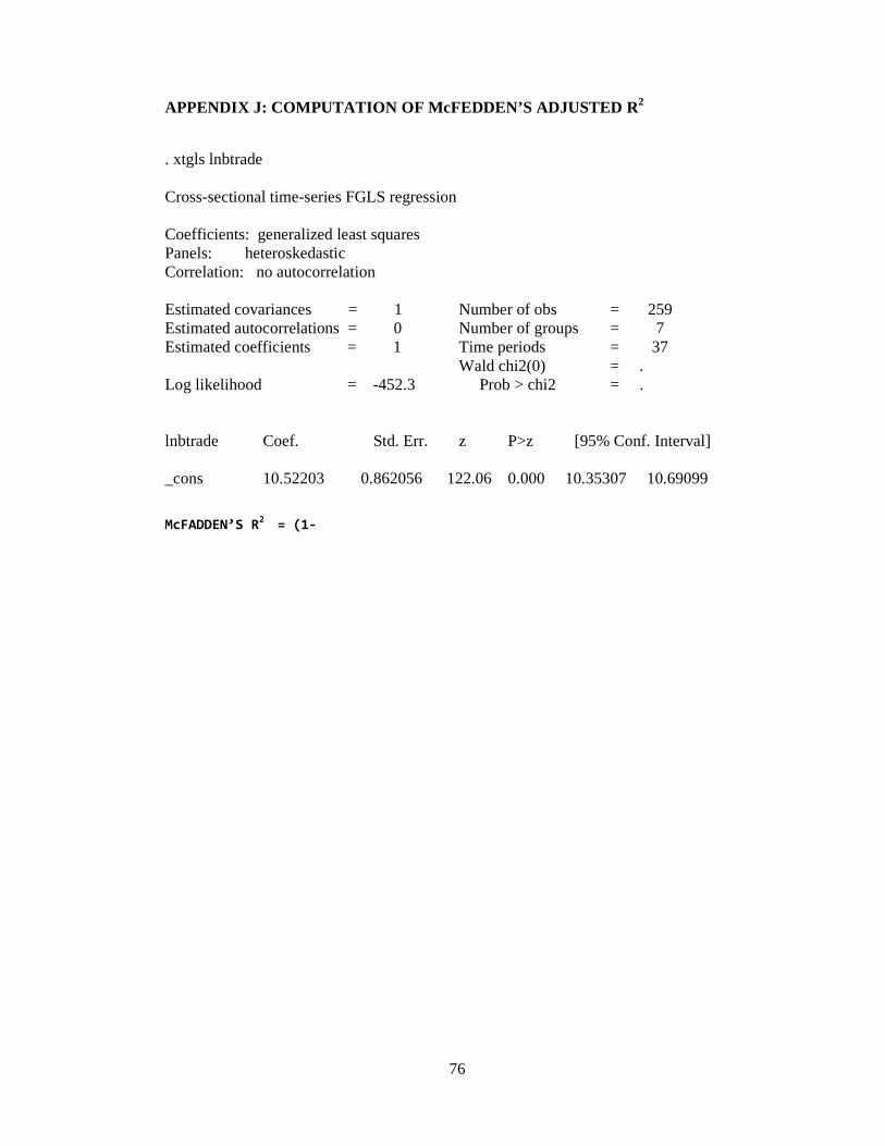
76
APPENDIX J: COMPUTATION OF McFEDDEN’S ADJUSTED R 2
. xtgls lnbtrade Cross-sectional time-series FGLS regression Coefficients: generalized least squares Panels: heteroskedastic Correlation: no autocorrelation Estimated covariances = 1 Number of obs = 259 Estimated autocorrelations = 0 Number of groups = 7 Estimated coefficients = 1 Time periods = 37
Wald chi2(0) = . Log likelihood = -452.3 Prob > chi2 = . lnbtrade Coef. Std. Err. z P>z [95% Conf. Interval] _cons 10.52203 0.862056 122.06 0.000 10.35307 10.69099
McFADDEN’S R2 = (1-