factors associated to poverty mobility in greater buenos ... · luis beccaria and roxana maurizio...

Factors associated to poverty mobility in Greater Buenos Aires*/ **/

Luis Beccaria and Roxana Maurizio Universidad Nacional de General Sarmiento

Argentina 2006

Abstract This document studies the dynamics of poverty between 1991 and 2003 in Greater Buenos Aires. It identifies and analyses the impact of different events that are associated to poverty entries and exits. The effect of inflation on real income change is also identified. Data of the Argentine’s household survey is employed and the methodology includes a correction for attrition. The results that were reached reinforce the view of sizeable entries and exit rates associated to the high incidence of poverty. Episodes related to the labour market proved to be the most important as they were more frequent and had an important impact on incomes. Those events of demographic character, however, were scarcely relevant. Keywords: poverty, entry and exit rates, dynamic information, labor and demographic events. JEL Classification: I32, J60

Resumen El documento analiza la dinámica de la pobreza entre 1991 y 2003 en Gran Buenos Aires. En particular, identifica el impacto de diferentes eventos asociados a las entradas y salidas de la pobreza, incluyendo el efecto de la inflación. Los datos provienen de la EPH y fueron corregidos por attrition. Los resultados muestran que los eventos relacionados con el mercado de trabajo son los de mayor importancia en las transiciones entre pobreza y no pobreza, tanto por su mayor frecuencia como por su mayor impacto sobre los ingresos familiares. Por el contrario, los eventos de carácter demográfico parecen tener escasa relevancia en la dinámica de la pobreza. */ A previous version was presented at the Workshop on Povety and Social Exclusion Dynamics, University of Vigo (July 2005) **/ Ana Laura Fernández and Paula Monsalvo were of great help in preparing this document by collaborating in data processing.

Introduction In October 2002, the incidence of poverty, measured according to the absolute poverty line method, reached 54.3% of the population of Argentina, by far the highest level ever recorded. Although the sharp rise that took place in the first half of 2002 –after the peso devaluation and the consequent rise in inflation– certainly contributed to that record, the incidence of poverty had been growing since 1994, pushed by the lack of dynamism in the labour market and increasing income inequality. Average poverty incidence during the nineties was much higher than in previous decades, thus pointing to an upward long-run behaviour. From 2003 onwards, in the midst of a process of rising employment and –to a lower extent– real wages, the growing trend of poverty incidence was reverted. By the end of 2005, poverty incidence reached figures similar to those of 2001. Even though the crisis that started in 1998,-which became particularly profound after the change in the macroeconomic regime- has been overcome, the social situation is still very difficult. The persistence of conditions of extreme vulnerability over long periods of time explains why the improvement in macroeconomic performance and in labour market variables, has not been sufficient so far to modify the situation of social deprivation that still affects a large share of total population. Therefore, it seems important to obtain and discuss evidence on the factors affecting poverty. Even though there is a considerable literature on this subject in Argentina,1 most of the analyses make use of static data and there is little experience regarding dynamic analyses. This document aims to contribute to this literature by studying the dynamics of poverty between 1991 and 2003 in Greater Buenos Aires (GBA), period during which poverty rose continuously. Since the selected period witnessed phases of expansion and recession, it is convenient to link the evolution of poverty incidence to labour market developments. In this sense, the paper analyses how changes in the poverty situation of households are related to labour market events (such us, for example, leaving or entering occupations, changes in the number of hours worked, changes in labour and non-labour incomes) and to those of demographic nature (among them, alterations in the size and composition of households). Specifically, it aims at assessing the relevance of different events experienced by households’ members that resulted in changes of incomes that might have led them to enter or leave poverty. It is the first contribution to poverty analysis in Argentina that links different labour market and demographic events to poverty dynamic. The data used come from the Permanent Household Survey (EPH). The analysis has been restricted to GBA –the largest Metropolitan Area in the country, where one third of total population lives– due to data constraint: only micro data of this region are available for the complete period of analysis

1 See, for example, Paz (2005) and Cruces and Wodon (2003)

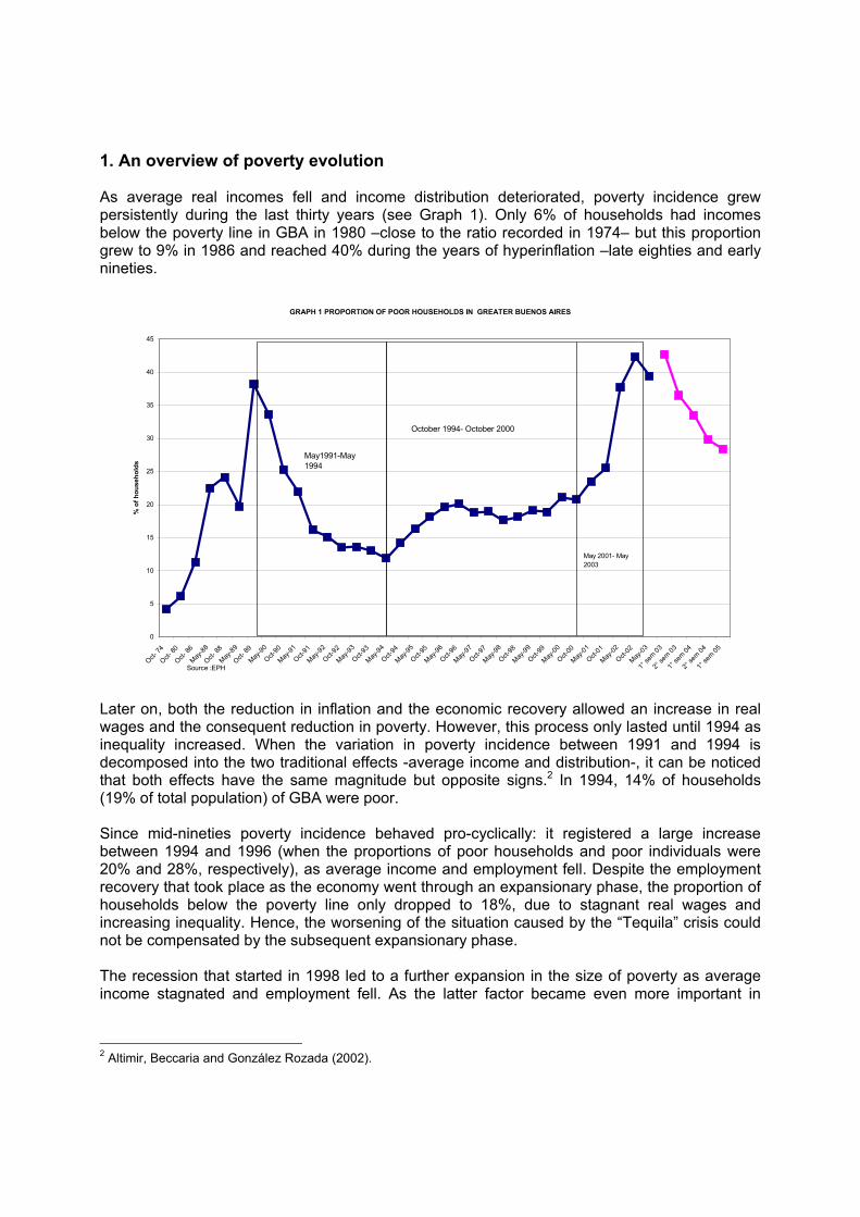
1. An overview of poverty evolution As average real incomes fell and income distribution deteriorated, poverty incidence grew persistently during the last thirty years (see Graph 1). Only 6% of households had incomes below the poverty line in GBA in 1980 –close to the ratio recorded in 1974– but this proportion grew to 9% in 1986 and reached 40% during the years of hyperinflation –late eighties and early nineties.

GRAPH 1 PROPORTION OF POOR HOUSEHOLDS IN GREATER BUENOS AIRES

0

5

10

15

20

25

30

35

40

45

Oct- 74

Oct- 80

Oct- 86

May-88

Oct- 88

May-89

Oct- 89

May-90

Oct-90

May-91

Oct-91

May-92

Oct-92

May-93

Oct-93

May-94

Oct-94

May-95

Oct-95

May-96

Oct-96

May-97

Oct-97

May-98

Oct-98

May-99

Oct-99

May-00

Oct-00

May-01

Oct-01

May-02

Oct-02

May-03

1° se

m 03

2° se

m 03

1° se

m 04

2° se

m 04

1° se

m 05

% o

f hou

seho

lds

May1991-May 1994

October 1994- October 2000

May 2001- May 2003

Source :EPH

Later on, both the reduction in inflation and the economic recovery allowed an increase in real wages and the consequent reduction in poverty. However, this process only lasted until 1994 as inequality increased. When the variation in poverty incidence between 1991 and 1994 is decomposed into the two traditional effects -average income and distribution-, it can be noticed that both effects have the same magnitude but opposite signs.2 In 1994, 14% of households (19% of total population) of GBA were poor. Since mid-nineties poverty incidence behaved pro-cyclically: it registered a large increase between 1994 and 1996 (when the proportions of poor households and poor individuals were 20% and 28%, respectively), as average income and employment fell. Despite the employment recovery that took place as the economy went through an expansionary phase, the proportion of households below the poverty line only dropped to 18%, due to stagnant real wages and increasing inequality. Hence, the worsening of the situation caused by the “Tequila” crisis could not be compensated by the subsequent expansionary phase. The recession that started in 1998 led to a further expansion in the size of poverty as average income stagnated and employment fell. As the latter factor became even more important in

2 Altimir, Beccaria and González Rozada (2002).

2001, the incidence reached a very high figure by the end of the year: 26% of households and 35% of population (28% and 38%, respectively, for all urban areas).3 By the end of 2002, poverty incidence reached 42% of households (54% of total population), in part because employment continued falling but, especially, due to the drastic erosion of real incomes that followed devaluation and the consequent rise in prices. This serious worsening of the social situation that followed the collapse of the currency board exchange regime –the Convertibility Plan– is not only explained by the magnitude of the shock –measured in terms of the size of income and employment reduction– but also by the extreme vulnerability of the distributive situation prior to the change of regime. The Argentine economy was already characterised by very low incomes, high unemployment and an unequal income distribution, with a large proportion of the non-poor population with incomes close to the poverty line. The favourable behaviour of the labour market since 2003, allowed a downward trend in poverty incidence. Even though it fell from 52% to 38% during the following two years (measured in terms of persons), it still remained at a very high level, indicating the persistence of a very difficult social situation. 2. Methodology and information source

2.1 The source of information

Data used in this paper come from the regular household survey of Argentina, the Permanent Household Survey (EPH) carried out by the National Statistical Office (INDEC), which covers urban areas and collects information especially on labour market variables. Until 2003 it was carried out twice a year in 31 urban centres, during May and October.4 Even though the EPH is neither a longitudinal survey nor does it include retrospective questions, its rotating panel sample allows to draw flow data from the survey, i.e. a selected household is interviewed in four successive moments or waves. Consequently, by comparing the situation of a household (or individual) in a given wave to that of the same household in the following one, it is possible to assess if the household has experienced changes in diverse variables, including occupational and demographic variables. The sample is comprised by four panels. In each wave, one panel enters the sample while other leaves it, i.e. one quarter of total households interviewed is renewed in each wave. Therefore, it is possible to compare 75% of the sample between two successive waves. Data from EPH can be used to trace the situation of a given household along the periods during which it is interviewed. For example, for a given unit that was poor in the initial period it is possible to know whether it remained in poverty or left such condition. Each household may also be characterised by a series of demographic and socioeconomic attributes. In particular, the households’ members can be classified according to labour market variables, thus making it possible to link changes in this dimension to modifications in the households’ living conditions. In this paper we analyse information of GBA in the 1991-2003 period. This restricted geographical coverage owes to the lack of microdata surveyed by EPH for all urban areas

3 There was only one official poverty line until 2001, for GBA. The release of official measures of poverty incidence began in 1986. The figures for 1974 and 1980 mentioned above were taken from Altimir and Beccaria (1998) and were estimated using the same criteria and procedures used in the official estimates. 4 In 2003, the survey underwent some changes and is now producing quarterly estimates. For a description of the survey’s methodology, see INDEC (1996).

previous to 1995. Transitions to be analysed are those resulting from comparing two successive waves, i.e. May and October or October and May.

In order to have enough observations, transitions of the entire 1991-2003 period –and of certain sub-periods– were pooled. Consequently, a given household could appear up to three times in the pool. The total number of observation included in the pooled panel was of 31.589.

In addition to the limitations just mentioned, data on movements coming from this source face other restrictions. One of them derives from the presence of data attrition due to different reasons –e.g. households moving to new homes, persons deciding to leave the panel, difficulties in the field work. This causes the effective proportion of individuals and households that are actually matched in two successive waves to be lower than the theoretical proportion (75% for the sampling design). Even though the number of observations left in the pooled panel is still sufficient, the mentioned phenomenon may be not random and, consequently, introduce biases. As will be mentioned in the next heading, a correction was considered during estimation. Another difficulty arises from the fact that not every movement can be captured when matching two successive waves. Since a transition is identified by comparing two observations in a five/seven-month span, two or more symmetrical changes between poverty and non-poverty would not be identified. 2.2 Methodology Different methods and models has been employed when analysing poverty dynamics. Some of them model income mobility and poverty dynamics is derived from such analysis; this is the case of the covariance structure model developed by Lillard and Willis (1978). Another widely used approach is that of the hazard models for poverty entry and exits that takes into account duration of different spells (Stevens, 1999; Devicenti (2001)). It can also be identified those analyses that aim at obtaining unbiased estimates of transitions between poverty and non-poverty by jointly modeling entry and exit probabilities, inicial poverty status and non-random atrition. Cappellari and Jenkins (2002a) used a trivariate probit in order to account for both sources of endogeneity (the initial status in t and panel retention between t and t+1) in addition to the modeling of the poverty transitions between t and t+1.5 As Capellari and Jenkins (2002a) mentioned, each of these approaches faces advantages and limitations, For instance, covariance structure models assume the same income dynamics for all households, poor and non poor, a situation scarcely probable. Hazard models, which introduce non-linearities by distringuish poor and non-poor, have typically ignored the types of endogeneity above mentioned. Finally, trivariate and bivariate models may face identification problems because of the difficulties for finding an adequate instrument. For modelling the initial conditions, the instrument should be a variable that affects the probability of being poor at t but does not affect the probability of transition in and out of poverty between t and t+1 (initial conditions); for modelling attrition a variable that affects the probability of retention between t and t+1, but does not affect the probability of transition, is needed. Our research project aims at estimating unbiased poverty entry and exit rates associated to

5 Stewart and Swaffield (1999) modeled transitions into and out of low pay using a bivariate probit model with endogenous selection. Cantó et al (2002) applied a bivariate probit model with selection equation.

different events by considering a trivariate model that takes into account both attrition and endogeneity of initial conditions. Such approach is still under study given the difficulties for identifying valid instruments from the variables measured in the household survey. In this paper it was only possible to correct for attrition through a method based on the re-wighting of the observations (see below). It was only applied when estimating overall exit and entry rates but not for those associated to different events. Firstly, entry and exit poverty rates are analysed in order to assess the importance of these movements on poverty incidence change. Then, we study the relationship between these transitions and occupational and income instability. The entry rates are calculated as the proportion of non-poor households in “t” that become poor in “t+1”. The exit and the permanency rates are computed similarly. As it was indicated above, for the 1991–2003 period the rates were calculated from a pool combining the transitions from consecutive May and October waves, and consecutive October and May waves. These rates are consistent estimators of probabilities.6 As mentioned, the estimation of these overall rates are corrected for attrition by a re-weighting of the observations. Such method uses a probit regression of the probability of staying in the panel in two successive waves, considering the household’s head attributes and households’ characteristics as explanatory variables. The new weights were estimated adjusting the original weights by the inverse of the predicted probability of being a “stayer”. The sum of the new weights are constrained to the total number of households in the first wave.7 This paper focuses on the economic and demographic events that trigger poverty entries and exits. For that purpose, we identify certain situations faced by households and we relate them to changes in their poverty condition. Two approaches have been followed in the literature in order to assess the importance of each event.8 One of them studies mutually exclusive events, whereas the other analyses the significance of a given event, even if it is verified simultaneously with other events. In this document we employ the first of these two alternatives. However, we still need to consider categories indicating the combination of two or more events in order to cover all (i.e. 100% of) cases. Therefore, we estimate the distribution of poverty transitions associated to given mutually exclusive events (or a combination of events). In this sense, it is important to remark that these events are not interpreted as factors of transitions –exogenous events- but only as events associated to transitions Following Jenkins and Shulter (2001), such distribution can be decomposed into two factors: on the one hand, the probability of the population at risk -e.g. non-poor households when analysing transitions to poverty– of experiencing such an event. The second factor consists of the conditional probability of the event triggering poverty entries or exits, given that the event has occurred. Entry (S1) and exit (S2) rates correspond to the probabilities of moving from state i/j in period “t” to state j/i in “t+1”, whereas the states are “poor” and “non–poor”. It is therefore not trivial to quantify the impact of different events on the probability of the transition.

6 The characteristics of the sample, jointly with the construction of mutually exclusive events –poor , non poor–, allow to associate a multinomial distribution to the quantities of ‘entries to’ and ‘exits from’ poverty. Therefore, consistent estimation of the probabilities of entering or exiting poverty (pij) has been reached by optimization of the likelihood function, which results in the relative frequencies of the transitions. 7 For a detailed description of this methodology, see Cantó et al (2006) 8 See, for example, Bane and Ellwood, (1986), Antolín et al (1999), Cantó et al (2002).

In order to do so, we use the partition and additivity properties of the sample space of mutually exclusive events. Assuming that the space is partitioned in R mutually excluding events, the probability of moving form the state “i” to the state “j”, (Sij) is equal to the sum of probabilities of all the events that comprise the sample space. That is to say,

∑=

=R

rrijij eventSPSP

1),()( [1]

Where: Sij, is the transition from state “i” in “t” to state “j” in “t + 1”. r: 1,2,…,R i ≠ j This probability can be also formulated as follows:

)()|()(1

r

R

rrijij eventPeventSPSP ∑

=

= [2]

where eventr indicates the occurrence of event “r”. This reparametrization of the transition probability makes it possible to assess the impact of each event on the probability of transition between states. In countries like Argentina, which experienced periods of high inflation, it is necessary to consider inflation as a factor leading to poverty transitions, since rising prices may affect real incomes pushing the households into poverty, or preventing them from exiting poverty. Consequently, the probability of transition (Sij) will be calculated taking this factor into account. In order to evaluate the impact of inflation on poverty transitions, households entering poverty can be partitioned into two groups: on the one hand, those households which became poor without going through any event that could lead to a reduction in the nominal income per adult equivalent (ipae); i.e. those households that fell into poverty only due to the effect of inflation. On the other hand, the second group comprises households that have not only been affected by inflation but also by at least one event. Hence, the entry probability can be expressed as follows:

∑∑==

Π∩Π∩+Π∩Π∩=R

rrrij

R

rrrijij eventPeventSPeventPeventSPSP

11)()|()()|()( [3]

Where i, j = non-poor, poor

revent : indicates that event “r” does not occur Π : indicates inflation

As those households experiencing events that lead to reductions in ipae are also affected by inflation, it is worthwhile to quantify the importance of each factor. The only possible way of doing this is through counterfactual estimations because only the jointly effect of both factors can be observed. In particular, this requires counterfactual estimations that consider one of these factors as fixed: This can be made by disaggregating the probability of entering poverty for those experiencing an event into three probabilities. • the probability of a household entering poverty because it is affected to a greater extent by

the impact of the event than by inflation –i.e. it would have entered poverty even if the nominal poverty line had remained constant. This can be estimated by computing the counterfactual probability of becoming poor by replacing the poverty line of the second observation with the poverty line of the first observation.

• the probability of a household entering poverty even if no reduction in its ipae occurs. Again, a counterfactual probability is computed by replacing total ipae of the second observation with that of the first one.

• the probability of a household entering poverty due to both factors: a diminishing ipae and inflation. The magnitude of this probability is derived as a residual.

Consequently, the second term of [3] can be expressed as follows:

residualeventPeventSP

eventPeventSPeventPeventSP

rrij

R

rrrij

R

rrrij

+

+Π<Π<+

+Π>Π>=Π∩Π∩ ∑∑==

)()|(

)()|()()|(11

[4]

where the sign > or < indicates that the importance of the event is greater or less than the importance of inflation. While inflation may by itself lead to poverty entry, it may also prevent an exit from occurring. In order to assess how each event affects the exit probabilities when inflation is considered, it is necessary to estimate a “counterfactual” exit probability (P*ij). This probability takes into account not only those households actually leaving poverty but also those that, despite experiencing events that increased ipae, were not able to exit poverty because such increase was lower than inflation. This counterfactual probability is computed by maintaining the poverty line of the first observation in the second observation. Hence, this counterfactual probability could be expressed as follows:

∑=

Π∩Π∩=R

rrr eventPeventSjiPSjiP

1

* )()|()( [5]

where Π indicates a situation of no inflation. Therefore, that probability comprises the probability of exiting poverty even when inflation occurred –i.e. the probability of households experiencing an increase in their incomes that is

higher than the increase in their poverty lines– and the rest, i.e. the probability of leaving poverty had the poverty line remained constant. Consequently, [5] could be expressed as follows:

∑=

+Π>Π>=R

rrr residualeventPeventSjiPSjiP

1

* )()|()( [6]

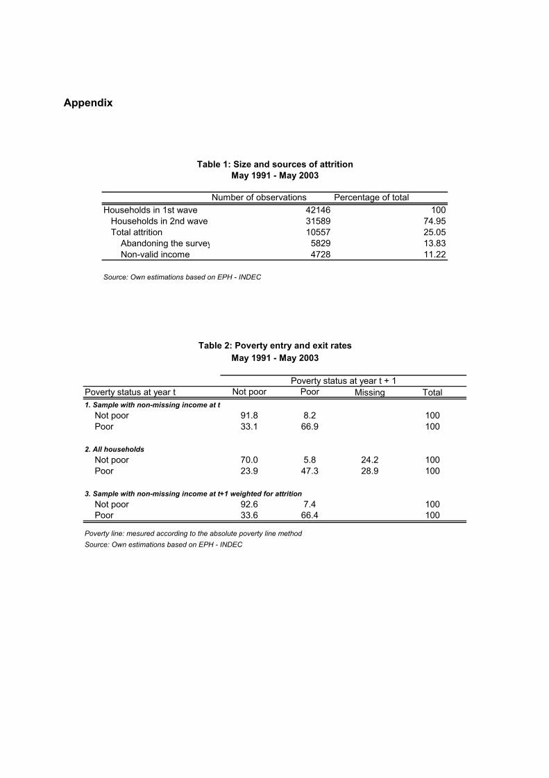
The relevance of the different events associated to transitions can also be analysed using regression models. Specifically, logit models wich consider the identified events as covariable will be estimated. Certain attributes of the households will also be included in the set of covariables for controlling their influence beyond the presence of the events. A variable that usually turns to be relevant -and that will be considered in these models- is the distance between households’ income and the poverty line.9 3. The dynamics of poverty in Argentina 3.1. Entry and exit rates As indicated, an attempt was made for correcting the effect of attrition on the estimates of entry and exit rates. For the panel of observations of households that should remain in two successive waves (i.e. excluding those leaving the survey panel given the survey’s rotation scheme), 25% of households did not have income information in the second wave. This wastage –of a non-random character– is due to two reasons: households abandoning the survey (14% of cases) and households remaining in the survey but with non-valid income –11%– in the second wave (due to total or partial non-response to questions of incomes) (Table 1). In both situations it is not possible to define the poverty status of the household in the second wave. Table 2 indicates the different size of these two sources of attrition for initially poor and non-poor households, being higher for the former group. The effect of correcting for attrition does not appear to be important for exit and only mildly significant for entries, whose rate decreases in approximately 1 pp for the whole period.la cual disminuye en cerca de un punto porcentual en el período completo (Table 2). This same feature is observed for each of the different subperiods. For observations weighted for attrition, data show that the entry and exit rates between observations separated by the six-month span averaged 7.4% and 33.6%, respectively, during the entire 1991-2003 period (Table 3). As expected, the probability of being poor in a given period is conditioned by the status of the previous observation; however, it must by stressed that this evidence of high persistence is not controled by heterogeneity. As it was already mentioned, inflation provokes downward movements in real incomes, thus modifying those movements coming from changes in nominal figures (which are derived from alterations in the number of earners and/or in the hours worked and/or in nominal earning rates). Hence, it is worth identifying the impact of inflation on the magnitude of poverty flows. This can be deduced by comparing the just mentioned figures with those computed when considering no price-change (specifically, considering no change in the value of the poverty line). When doing so, the entry and exit rates become 6.8 % and 35.6% respectively, indicating that during these periods the main sources of movements came from changes in nominal ipae (Table 3).

9 These models can, in turn, suffer from a bias –the effects of this will not be considered here– derived from a certain endogeneity of the covariables, since a change in poverty condition may influence some of them.

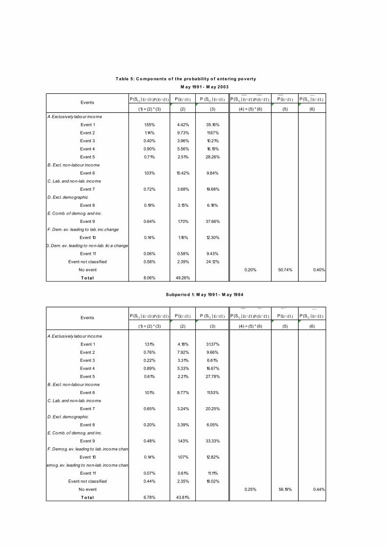
Given the different trajectories of poverty incidence during the entire period (see Section 2), it is convenient to distinguish between homogeneous sub-periods. Consequently, estimates were made for the following phases: May 1991-May 1994; October 1994-October 2000 and May 2001–May 2003. The entry rate grew systematically along the whole period, whereas the exit rate showed the opposite behaviour, as it was expected during a period of increasing poverty incidence. This rise in poverty incidence was, therefore, associated to an increasing duration of poverty episodes -the exit rate halved– and to larger flows towards such condition, being the former the most important of both factors (Table 3). Even if the effect of inflation was not significant during the sub-periods considered, there are some differences between them: it was higher in the first and the last sub-periods, while there was almost no effect from 1994 to 2000, when prices remained almost constant (Table 3).10 3.2. Events related to poverty transitions As it was pointed out, the main objective of this contribution is to analyse the importance of diverse events experienced by households as factors causing entries to and exits from poverty. As indicated en 2.2, we will use mutually exclusive events that refer to single or combined episodes. In order to define the classification of events, consider the situation of a household leaving poverty. Such transition occurs if its total nominal income rises, if the number of members falls, or due to a combination of both episodes leading to an increase in the ipae. These movements are the consequence of different events experienced by the household. The rise in a household’s total nominal income can be the result of one member getting a job or facing a wage increase while, for example, the death of a member leads to a smaller household. Therefore, we first distinguish between the latter type of events –of demographic character– and the others. Among the others, we consider those exclusively related to labour market events or to non-labour income events. We also take into account those episodes affecting simultaneously labour and non-labour incomes. However, some events lead to an exit from poverty by affecting both, the nominal income and the size of the household –e.g. the arrival of an adult-employed person to the household that increases the nominal ipae; hence, this type of events are of both demographic and non-demographic character. We take into account such situations by identifying combined events. The procedure is similar for entries to poverty. The identified events are the following: A. Exclusively labour income events

1. Growth / reduction in the number of employed persons not linked to an entry / exit of labour income earners to the household, maintaining the total number of household members;

2. Growth / reduction in total hourly wage of members employed in both observations, maintaining the total number of household members and worked hours;

3. Growth / reduction in the number of worked hours of members employed in both observations, maintaining the total number of household members and hourly wage;

4. Growth / reduction in the number of worked hours and in the total hourly wage of members employed in both observations, maintaining the total number of household members;

10 The average monthly inflation rate was 1% in the first period, near zero in the second, and 1.4% in the third one.

5. Growth / reduction in the total monthly wage of members employed in both observations and in the number of persons employed, not linked to an entry / exit of labour income earners to the household, maintaining the total number of household members;

B. Exclusively non-labour income events

6. Growth / reduction in non-labour incomes not linked to an entry / exit of non-labour income earners to the household, maintaining the total number household members;

C. Labour and non-labour income events

7. Growth / reduction in labour and non-labour incomes not linked to an entry / exit of labour or non-labour income earners to the household, maintaining the total number of household members;

D. Exclusively demographic events

8. Reduction / growth in the total number of household members; total nominal income remains constant;

E. Combination of demographic and income events

9. Growth / reduction in total nominal income (irrespective of the source of income change) and reduction / growth in the number of household members;

F. Demographic events leading to labour income changes

10. Growth / reduction in the number of employed persons due to the fact that some employed members enter / leave the household;

G. Demographic events leading to non-labour income changes

11. Growth / reduction in non-labour incomes due to the fact that some non-labour income earners enter / leave the household;

20. Events not classified. A, B and C are non demographic events as the number of members in the household remains constant and there is no entries or exits of labour and non labour earners to or from the household. On the contrary, the rest of the events are exclusively demographic or a combination of demographic and non demographic factors. (a) Entries One half of total households in GBA have not experienced an event leading to a reduction in ipae during the whole period (Table 5, column 5). It is worth mentioning that those households who have witnessed a reduction in their ipae but could not be classified in any of the categories considered represent a very small proportion (0.4% of total households and 0.8% of those that have reduced their ipae) (Table 5, column 2). Approximately 58% of total entries to poverty during the entire period are explained by events exclusively related to the labour market. Therefore, among single events, this type of event is the most important one. When considering all the combined events that include at least one event related to the labour market, such figure reaches 81% (Table 4). Households only showing a reduction in non-labour incomes –that basically reflect pensions received by retired persons–

also account for an imporant proportion of total entries –12%–. The increase in the number of members is, per se, an event causing a low proportion of entries to poverty (2%). Therefore, exclusively demographic events do not appear to be relevant. Other demographic events leading to, or being accompanied by, labour and/or non-labour income reductions account for 14% of total entries. Among the individual labour market events, the reduction of the number of employed members is the most important one. The fall in wage rates also appears as relevant, while the reduction in the number of hours is less significant. However, the combination of changes in wage rates and hours, and the combination of less employed members and wage rates reductions, show relatively high proportions (Table 4). The importance of the sum of all individual labour market events in causing transitions to poverty described above is mainly derived from their relatively high frequency of occurrence –more than one quarter of total non-poor households experienced exclusively an episode of this type. The average conditional probability of these events causing an entry to poverty is similar to the average of all possible events. Even if the reduction in the number of employed persons is the individual event causing more entries (Table 4), this is primarily due to its larger conditional probability. For example, the reduction of wages is an event even more frequent but with a lower conditional probability (Table 5). In general, single labour market events have larger probabilities than single non-labour incomes and demographic related episodes. In particular, while a reduction in non-labour incomes is a relatively usual situation for a household –it is the most frequent of the identified events, single or combined–, the probability that such event pushes a household into poverty is low (around one half of the average of all events). Therefore, this event explains a lower proportion of entries (12%) than the proportion of total events (21%). The lack of importance of demographic events is associated with low frequency but, especially, with low conditional probability. Finally, as expected, all combined episodes: labour and non-labour; labour and demographic; or labour, non-labour and demographic, have a larger probability of pushing a household into poverty, but are less frequent. Relative values of conditional probability of each event are confirmed by a logit model (Table 6). Apart from controlling for socio-demographic variables –which have the expected influences–, one of the regressions (model 2) also controls for the distance between the households’ income and the poverty line. The conditional probabilities are larger in the latter case than in model 1 (the model that does not include the “distance variable”). This result would indicate that many households experiencing an event and with incomes well above the poverty line do not enter poverty because the reduction in their ipae is not enough. Hence, the average conditional probabilities are higher when controling for distance. The effects of each type of event on entry rates previously discussed also include those provocked by inflation. However, the impact of the latter is very low: 92% of total entries would have occurred even with no inflation. Furthermore, two thirds of those households that entered poverty because of price increase also experienced an episode that reduced their ipae (Table 4). The proportion of events that reduce ipae rose through time –from 44% in the first sub-period to 54% in the third– and labour market episodes made contribution proportional to their importance (Table 5). This result could be reflecting, on the one hand, the fall in nominal incomes during 1998–2001 that was to some extent related to movements between jobs –with or without an unemployment episode in between– experienced by some workers in a labour market with high

turnover.11 The impact of the reduction in worked hours may be manifesting the growth in the rate of hourly underemployment, which peaked during 2000-2002. The significant increase in the unemployment rate that characterised the whole period explains the relevance of an occupation loss as a source of unemployment. The overall increase in the entry rate between the first and the third sub-period was explained by that rise in the occurrence of income-reducing events but also in the average conditional probability of causing a household to enter into poverty.12 In fact, the relative importance of labour market grew not only due to the increase in the frequency of these events but also because of the greater conditional probability. In particular, the frequency of the loss of employed members maintained constant but their impact increased significantly, similar to what happened with worked hours; as the same time, there was a increase in the share of wage reduction events and a higher incidence of these reductions was also noted. These results manifest the increasing difficulties of the labour market during the whole period. A decomposition exercise of the increase in the entry rate between these sub-periods shows that the first of these two sources accounts for 49% of the increase, while 63% is due to the rise in the conditional probabilities (a negative interaction term of 12% results). The size of the latter effect is directly related to the magnitude of the income reduction caused by the event but inversely related to the distance between the households’ income and the poverty line. The table below shows the average value of two variables that try to capture both effects for the first and third subperiod; it was computed for all households that were non-poor in the first observation and that have experienced an event.

Sub-period 1 Sub-period 3Relative distance between the household income and the poverty line 1/ 4.21 4.11Change in household income relative to the poverty line 2/ -1.12 -1.05

1/ ITF/PL1, where PL1 is the value of the poverty line in the first wave2/ (ITF2 - ITF1) / PL1

It appears that the average distance has changed in the expected direction but in a small magnitude while average change in income was similar in both sub-period. The share of labour market events among those leading to a reduction in income per adult equivalent did not change between the first and the third sub-periods. Hence, the increasing proportion of poverty entries of these events indicates that their conditional probabilities grew more than average probability. The events whose impact increased the most are the reduction in wage rates and in the number of hours. Among the rest, the fall in non-labour incomes constitutes an episode that gained relative presence but did not change its conditional probability.

11 Beccaria and Maurizio (2005) 12 The rise of the conditional probability is not explained by changes in the distribution of events.

(b) Exits Like in the case of entries, labour market events are of great importance for explaining exits from poverty and, in fact, they account for a similar proportion to that of entries (59% for the whole period) (Table 7). Also, an increase in non-labour incomes appears as relevant (15%) while those exclusively demographic are of scarce importance. Since the average conditional probability of labour market events is similar to the average of all types of events, the importance they have in the distribution of events and in the distributions of exits from poverty are also similar. However, like it happens with entries, such probabilities are high for individual labour market events. The increase in non-labour incomes has, in this case, a large conditional probability, similar to the average of all events for the whole period (Table 8). Among poor households in the first observation, a third did not experience any event causing an increase in their ipae. Again, almost all of those households whose ipae grew between both observations (98%) could be classified according to the groups of events above mentioned. Comparing these results with those for entries, we can observe that the conditional probabilities of exits are higher than the entries. It is mainly due to the fact that initially poor households are closer to the poverty line than initially non poor household. A logit model –similar to that estimated for entries– results in relative conditional probabilities of exiting poverty similar to those showed in Table 6. The coefficients for the events rise when the poverty gap is included, suggesting that households experiencing an event, but with very low incomes are not able to exit from poverty because their ipae do not increase sufficiently (Table 9). The exit rate fell throughout the three sub-periods leading, as it was indicated, to an increase in the duration of poverty episodes. Such performance was due to reductions in both the occurrence of events causing a rise in households’ ipae and in the average conditional probability of the events that take a household out of poverty (Table 8). The results for the case of exit rates of the same decomposition exercise conducted for entry rates changes indicate that the reduction in the conditional probabilities was the main factor explaining the overall fall in the probability of leaving poverty; it explains 72% of such reduction. The decrease in the proportion of households undergoing an income-rising episode accounts for 18%, with an interaction component of 10%. Like in the case of entries, the change in the conditional probability of leaving poverty depends on those changes occurring in the variation of households’ incomes and in the initial distance between income and the poverty line. As can be seen in the figures below, the latter became larger while the average increase in ipae between the first and the second observation was smaller in the third sub-period than in the first one, being this effect the most important of both.

Sub-period 1 Sub-period 3Relative distance between the household income and the poverty line 1/ 0.66 0.51Change in household income relative to the poverty line 2/ 1.00 0.45

1/ ITF/PL1, where PL1 is the value of the poverty line in the first wave2/ (ITF2 - ITF1) / PL1

Finally, the proportion of labour market events in the distribution of exits was the same in the first and third period since the conditional probability of this type of events fell in a similar way than the average probability; in addition, their share in the distribution of events remained fairly constant between these periods.

4. Summary and conclusions Poverty is still a main concern in Argentina, where at least one third of its population lives in households with incomes below the poverty line. Furthermore, income instability appears to be, as in other countries of the region, relatively high, mainly linked to an unstable labour market characterised by a high incidence of unemployment and precariousness. In this context, the design of policies aimed at increasing incomes and reducing instability is an important issue since, at present, there is no employment or social program of wide coverage –like unemployment insurance or subsidies– that cushions the consequences of the cycle. Precisely, this paper tries to contribute to such discussion as it is a first attempt to identify different events that are usually associated to poverty entries and exits. Regarding methodological aspects, the paper presents a novel procedure to take into account the effect of inflation, even though during the period of analysis price rises did not play any important role. It also makes an attempt to control the estimates for attrition. Due to data restriction, the analysis was limited to the GBA and the 1991-2003 period. However, further information is expected in the future which would allow the broadening of the analysis. In particular, the period that started in 2003 is of particular interest given that poverty incidence fell quite rapidly from the very high levels reached in 2002. The results discussed in the paper not only reinforce the view that large entry and exit rates are associated to the high incidence of poverty, but specifically provide evidence on the relevance of different factors leading to changes in households’ incomes that make them fall into or get out of poverty. The episodes related to the labour market are the most important, both because of their frequency and their important impact on incomes. This result appears similar to results found in other studies for developed countries. However, Argentina appears differs from them as the relevance of demographic events is scarce. The evolution of poverty dynamics during the three sub-periods considered reflects the increasing difficulties experienced by the labour market during the nineties and the beginning of the present decade. The larger entry rates and lower exit rates were almost completely explained by the greater frequency of labour market events leading to income reductions –transitions to unemployment and reduction in wages– and to a lower occurrence of those that increase incomes. Furthermore, as income distribution worsened during the period under analysis, the income of an increasing number of non-poor households became closer to the poverty line, while the poverty gap of poor households also widened. This last factor, together with the relatively large changes in income associated to these events, caused the probability of falling into poverty when a negative event occurred to rise, and the probability of taking a household out of poverty when a positive event occurred to fall. From the policy point of view, these results give support to wider anti – poverty strategies that include not only the traditional money or in-kind transference to poor households. Even if they should remain as a central component of such interventions, a high priority needs to be attached to efforts aimed at preventing low and medium-low income workers from facing income reducing events, specially those having the larger chances of bringing their households into poverty. Increasing their probabilities for leaving poverty should be also an important part of such policies. It implies acting both at the supply and at the demand side of the problem: i.e. estimulating the creation of new jobs suited for those workers and assisting them in increasing their chances of getting available jobs (through training and or better employment services, for example). The level of wages has to be also considered as not always obtaining an employment insure leaving poverty.

References Altimir, O., L. Beccaria and M. González Rozada (2002) “La distribución del ingreso en

Argentina, 1974-2000”, in Revista de la CEPAL, N° 78: 55-8 Altimir, O. and L. Beccaria (1998) “Efectos de los cambios macroeconómicos y de las reformas

sobre la pobreza urbana en la Argentina” (en colaboración) in E. Ganuza, L. Taylor y S. Morley Política macroeconómica y pobreza en América Latina y el Caribe, PNUD, Ed. Mundi-Prensa, Madrid.

Antolín, P., T. Dang and H. Oxley (1999) “Poverty dynamics in four OCED countries”, Economics Deparment Working Papers N° 212, OECD.

Bane,M. and D, Ellwood (1986) “Slipping into and out of poverty: the dynamics of spells” in Journal of Human Resources, 21 (1).

Beccaria, L. and R. Maurizio (2005) “Changes in Occupational Mobility, Labour Regulations and rising precariousness in Argentina”, National University of General Sarmiento, Argentina.

Blumen, I., M. Kogan and P. McCarthy (1955) “The industrial mobility of labor as a probability process, Cornell University Press, Ithaca.

Burgess, S. and C. Propper (1998) “An economic model of household income dynamics, with an application to poverty dynamic among American women, CASE Paper N°, London.

Bucheli, M. and M. Furtado (2002) “Impacto del desempleo sobre el salario: el caso de Uruguay”, in Desarrollo Económico, N° 165

Cantó, O. (1996) “Poverty Dynamics in Spain: A study of transitions in the 1990s”, DARP Discussion Paper N° 15, London School of Economics, London.

Cantó, O. (2000) “Climbing out of poverty, falling back in: low incomes’ stability in Spain. Working paper N°13, Departamento de Economía Aplicada, University of Vigo, España.

Cantó, O., del Río, C. and C. Gradín (2002) “What helps households with children in leaving poverty? Evidence from Spain in contrast with other EU countries, Working paper 0201, Departamento de Economía Aplicada, University of Vigo, España.

Cantó, O., del Río, C. and C. Gradín (2006) “Poverty statics and dynamics: does tha accounting period matter? International Journal of Social Welfare, vol 15 (3).

Capellari, L. and S. Jenkins (2002a) “Modelling low income transitions”. Discussion Papers 288, German Institute for Economic Research, Berlin.

-----------(2002b)”Who Stays Poor? Who Become Poor? Evidence from the British Hosehold Panel Survey”, en The Economic Journal, 112 (4778): C60-C67.

Cox, D. (1972) “Regression Models and Life-Tables”, Journal Royal Statistical Society. May/Aug.

Cox, D. and D. Oakes (1985) Analysis of Survival Data, New York: Chapman and Hall. Cruces, G. y Q. Wodon (2003) “Transient and chronic poverty in turbulent times: Argentina

1995-2002” Economic Bulletin, Vol. 9, N° 3 Devicienti, F. (2001) “Poverty persistence in Britain: a multivariate analysis using the BHPS,

1991-1997”. ISER Working paper 2001-02. University of Essex, Colchester. Duncan, G. (1983) “The implications of changing family composition for the dynamic analysis of

family economic well-being. In Atkinson y Cowel (eds.) Panel Data on Incomes. Occasional paper N°2, London School of Economics, London.

Duncan. G., Gustafsson, Hauser, Schmauss, Messinger, Muffels, Nolan and Ray (1993) “ Poverty dynamics in eight countries”, Journal of Population Economics, 6, 215-34.

Girardo, A. E, Rettore and U. Trivellato (2002) “The persistence of Poverty: True Dependence or Unobserved Heterogeneity?. Some evidence from the Italian Survey on Hosehold Income and Wealth”, Dip. Di Scienze Statisiche, Universidad de Padova.

Goodman, L. (1961) “Statistical methods for the Mover-Stayer model”, Journal of the American Statistical Association, 56, 841-68.

Heady, Krause and Habich (1994) “Long and short term poverty: Is Germany a two-thirds society”, Social Indicators Research, 31, pp. 1-25.

Hausman, J. and A. Han (1990) “Flexible Parametric Estimation of Duration and Competing Risk Models”, Journal of Applied Econometrics, Vol. 5.

Heckman, J. and B. Singer (1984) “Econometric Durations Analysis“, Journal of Econometrics, Vol. 24.

Hill, M. (1981) “Some dynamic aspects of poverty, in Five Thousand American Families: Patterns of Economics Progress”. Analysis of the first twelve years of the Panel Study of Income Dynamics, Vol IX.

Hill, M. and S. Jenkins (1998) “Poverty among British children: chronic or transitory?, ISER Working Paper 1999-23, University of Essex, Colchester.

Jarvis, S. and S. Jenkins (1997) “Low income dynamics in 1990s Britain”, Fiscal Studies 18: pp.1-20.

Jarvis, S. and S. Jenkins (1999) “Marital splits and Income changes: Evidence from the British Household Panel Survey”, en Population Studies, 53: 237-254.

Jenkins, S. (1999) “Modelling household income dynamics”, ESRC Research Centre on Micro-Social Change, Working Paper 99-1, ISER, University of Essex, Colchester.

Jenkins, S. and Shulter (2001) “Why are child poverty rates higher in Britain than in Germany?. A longitunidal perspective”, Anglo

Jenkins, S. and Cappellari, L. (2002) “Modelling low income transitions”, ESRC Research Centre on Micro-Social Change, Working Paper N° 2002-8, ISER, University of Essex, Colchester

Kalbfleisch, J. and L. Prentice (1980) The Statistical Analysis of failure time data, Nueva York: Wiley.

Kiefer, N. (1988) “Economic Duration Data and Hazard Functions”, Journal of Economic Literature, Vol 26.

Lancaster, T. (1990) The Econometric Analysis of Transition Data, Econometric Society Monographs Nº 17, Cambridge: Cambridge University Press.

Layte, R. and C. Whelam (2002) “Moving in and out of poverty: the impact of welfare regimes on poverty dynamics in the EU”, EPAG Working Paper 2002-30, University of Essex, Colchester.

Lillard, L. and R. Willis (1978) “Dynamic aspects of earnings mobility”, Econometrica 46. McCall, J. (1971) “A Markovian model of income dynamics”, Journal of the American

Statistical Association, 66, 335, pp. 436-447. MacGinis, R. (1968) “A stochastic model of social mobility” American Sociological Review, 33,

pp. 712-721. Paz (2005) “Pobres pobres, cada vez más pobres. Una visión global de la pobreza”, in Mercado

de trabajo y Equidad en Argentina, Beccaria, L. and R. Maurizio (eds). Bs. As,. Prometeo. Pérez-Mayo, J. (2004) “Consistent poverty dynamics in Spain”, IRISS Working Paper Series, N°

2004-09 IRISS at CEPS/INSTEAD. Shorrocks, A (1978) “ Income inequality and income mobility”, Journal of Economic Theory,

19: pp. 376-93. Stevens, A. (1999) “Climbing out of poverty, falling back in. Measuring the persistence of poverty

over multiple spells”, in Journal of Human Resources, XXXIV: 557-588. Stewart and Swaffield (1999) “Low pay dynamics and transition probabilities”, Economica, 66. Walker, R (1994) “Poverty Dynamics: Issues and Examples”, Avebury, Aldershot.

Appendix

Number of observations Percentage of totalHouseholds in 1st wave 42146 100 Households in 2nd wave 31589 74.95 Total attrition 10557 25.05 Abandoning the survey 5829 13.83 Non-valid income 4728 11.22

Source: Own estimations based on EPH - INDEC

May 1991 - May 2003Table 1: Size and sources of attrition

Poverty status at year t Not poor Poor Missing Total1. Sample with non-missing income at t Not poor 91.8 8.2 100 Poor 33.1 66.9 100

2. All households Not poor 70.0 5.8 24.2 100 Poor 23.9 47.3 28.9 100

3. Sample with non-missing income at t+1 weighted for attrition Not poor 92.6 7.4 100 Poor 33.6 66.4 100

Poverty line: mesured according to the absolute poverty line methodSource: Own estimations based on EPH - INDEC

Poverty status at year t + 1

May 1991 - May 2003Table 2: Poverty entry and exit rates

Observed Counterfactual (*) Observed Counterfactual (*)

May-1991 - May-2003 Not poor 92.6 93.2 7.4 6.8 Poor 33.6 35.6 66.4 64.4


Oct-1994 - Oct-2000 Not poor 93.0 93.1 7.0 6.9 Poor 35.1 35.3 64.9 64.7


Poverty line: mesured according to the absolute poverty line method(*) Mantaining poverty line of the 1 st observation in the 2 nd observationSource: Own estimations based on EPH - INDEC

Table 3: Poverty entry and exit rates

Poverty status at year t Not poor PoorPoverty status at year t + 1

Sample with non-missing income at t weighted for attrition

__ __

P(Si j)=∑ [P(Si j | Ε∩Π)Ρ(Ε∩Π)+ P(Si j | Ε∩Π)Ρ(Ε∩Π)]

=P(Si j | Ε>Π)Ρ(Ε>Π)P(Si j | Ε<Π)Ρ(Ε<Π)+ residual(1 ) = (2) + (3) (2) (3) = (4) + (5) + (6) (4) (5) (6)

1.55% 1.49% 0.04% 0.03%1.14% 1.05% 0.08% 0.00%0.40% 0.36% 0.03% 0.01%0.90% 0.86% 0.02% 0.01%0.71% 0.68% 0.01% 0.01%

1.03% 0.94% 0.08% 0.00%

0.72% 0.69% 0.01% 0.02%

0.19% 0.17% 0.03% 0.00%

0.64% 0.62% 0.02% 0.00%

0.14% 0.14% 0.00% 0.00%

0.06% 0.06% 0.00% 0.00%

0.58% 0.55% 0.01% 0.01%

0.20%

Total 8.26% 0.20% 8.06% 7.62% 0.34% 0.11%

i = Non poor in 1st observationj = Poor in 2nd observationE = event__E = No eventObservatiosn not w eighted for attrition

C. Lab. and non-lab. income

D. Excl. demographic Event 7

Event 4Event 5

Event 6

Table 4: Probability of entering poverty

May 1991 - May 2003

A Exclusively labour income

B. Excl. non-labour income

Events

Event 1Event 2Event 3

No event

Event not classif ied

Event 8

Event 9

Event 10

Event 11

E. Comb. of demog. and inc.

F. Demog. ev. leading to lab. income changes

G. Demog. ev. leading to non-lab. income changes

__ __ __ __P(Si j | Ε∩Π )Ρ(Ε∩Π) P(Ε∩Π) P (Si j | Ε∩Π) P(Si j | Ε∩Π )Ρ(Ε∩Π) P(Ε∩Π ) P(Si j | Ε∩Π )

(1) = (2) * (3) (2) (3) (4) = (5) * (6) (5) (6)

1.55% 4.42% 35.16%

1.14% 9.73% 11.67%

0.40% 3.96% 10.21%

0.90% 5.56% 16.19%

0.71% 2.51% 28.26%

1.03% 10.42% 9.84%

0.72% 3.68% 19.68%

0.19% 3.15% 6.18%

0.64% 1.70% 37.66%

0.14% 1.16% 12.30%

0.06% 0.58% 9.43%

0.58% 2.39% 24.12%

0.20% 50.74% 0.40%

8.06% 49.26%

__ __ __ __

P(Si j | Ε∩Π )Ρ(Ε∩Π) P(Ε∩Π) P (Si j | Ε∩Π) P(Si j | Ε∩Π )Ρ(Ε∩Π) P(Ε∩Π ) P(Si j | Ε∩Π )

(1) = (2) * (3) (2) (3) (4) = (5) * (6) (5) (6)

1.31% 4.18% 31.37%

0.76% 7.92% 9.66%

0.22% 3.31% 6.61%

0.89% 5.33% 16.67%

0.61% 2.21% 27.78%

1.01% 8.77% 11.53%

0.65% 3.24% 20.25%

0.20% 3.39% 6.05%

0.48% 1.43% 33.33%

0.14% 1.07% 12.82%

0.07% 0.61% 11.11%

0.44% 2.35% 18.02%

0.25% 56.19% 0.44%

6.78% 43.81%

M ay 1991 - M ay 2003

Subperio d 1: M ay 1991 - M ay 1994

Event 1

Event 2

Event 3

Event 4

Event 5

T o tal


Event 7

D. Excl. demographic

Event 8

Event 11

Event not classified

No event

Events

Event 9

Event 10

Event 4

Event 5


Event 6



F. Dem. ev. leading to lab. inc.change

G. Dem. ev. leading to non-lab. Iic.e change

Event 1

Event 2

Event 3

Event 8


Event 9


Event 6


Event 7


No event

T o tal

Events


F. Demog. ev. leading to lab. income chang

Event 10

emog. ev. leading to non-lab. income chang

Event 11


T able 5: C o mpo nents o f the pro bability o f entering po verty

__ __ __ __

P(Si j | Ε∩Π)Ρ(Ε∩Π) P(Ε∩Π) P (Si j | Ε∩Π) P(Si j | Ε∩Π)Ρ(Ε∩Π) P(Ε∩Π) P(Si j | Ε∩Π)

(1) = (2) * (3) (2) (3) (4) = (5) * (6) (5) (6)

1.52% 4.39% 34.53%1.13% 10.38% 10.91%0.40% 4.09% 9.74%0.89% 5.66% 15.64%0.69% 2.52% 27.39%

0.92% 10.55% 8.75%

0.75% 3.84% 19.44%

0.16% 3.10% 5.10%

0.62% 1.70% 36.43%

0.13% 1.19% 10.64%

0.05% 0.58% 8.79%0.59% 2.47% 23.79%

0.04% 49.54% 0.09%7.83% 50.46%

__ __ __

P(Si j | Ε∩Π)Ρ(Ε∩Π) P(Ε∩Π) P (Si j | Ε∩Π) P(Si j | Ε∩Π)Ρ(Ε∩Π) P(Ε∩Π) P(Si j | Ε∩Π)

(1) = (2) * (3) (2) (3) (4) = (5) * (6) (5) (6)

2.13% 4.94% 43.07%1.81% 10.45% 17.33%0.76% 4.60% 16.49%0.98% 5.58% 17.54%0.95% 3.01% 31.71%

1.44% 12.85% 11.24%

0.76% 3.84% 19.75%

0.32% 2.94% 10.83%

1.00% 2.15% 46.59%

0.22% 1.25% 17.65%

0.05% 0.56% 8.70%0.66% 2.15% 30.68%

0.73% 45.65% 1.61%11.09% 54.35%

i = Non poor in 1st observationj = Poor in 2nd observationE = event__E = No event


Event not classif iedNo event

Total

Table 5 (cont.) Subperiod 2: Oct 1994 - May 2000

F. Demog. ev. leading to lab. incEvent 10

g. ev. leading to non-lab. incomeEvent 11


E. Comb. of demog. and inc.Event 9

B. Excl. non-labour income Event 6

C. Lab. and non-lab. incomeEvent 7

Event 2Event 3Event 4Event 5

No eventTotal

Events


Event 2

Event 10g. ev. leading to non-lab. income

Event 11Event not classif ied

Event 8E. Comb. of demog. and inc.

Event 9F. Demog. ev. leading to lab. inc

Event 6C. Lab. and non-lab. income

Event 7D. Excl. demographic



Event 1

Events

Event 1A Exclusively labour income

Subperiod 3: Oct 2000 - May 2003

Variables Model 1 Model 2Events

A Exclusively labour income Event 1 6.945 8.566

(16.79)** (20.08)** Event 2 5.458 6.741

(13.19)** (15.89)** Event 3 5.218 6.371

(12.34)** (14.63)** Event 4 5.824 7.487

(14.03)** (17.49)** Event 5 6.369 8.61

(15.22)** (19.85)**B. Exclusively non-labour income Event 6 5.857 6.776

(14.10)** (15.92)**C. Labour and non-labour income Event 7 6.25 8.228

(14.97)** (19.07)**D. Exclusively demographic Event 8 4.667 5.012

(10.69)** (11.24)**E. Combination of demographic and income Event 9 6.803 8.699

(16.13)** (19.90)**F. Demog. events leading to labour income changes Event 10 5.284 6.756

(11.83)** (14.38)**G. Demog. events leading to non-labour income changes Event 11 5.687 6.825

(11.47)** (13.20)**Event not classified 4.354 5.385

(5.94)** (6.66)**No event (omitted)

Control variables

EducationLess than incomplete primary 0.455 0.322

(6.29)** (3.76)**Complete Primary (omitted)

Incomplete secondary -0.549 -0.203(7.56)** (2.36)*

Complete secondary -1.029 -0.418(11.85)** (4.16)**

Incomplete terciary -1.407 -0.46(11.27)** (3.17)**

Complete terciary -2.245 -1.072(14.11)** (6.24)**

Male household head 0.245 0.109(2.82)** -1.07

Age of household head -0.025 -0.013(12.24)** (5.51)**

Number of members 0.208 -0.073(12.42)** (3.47)**

Married couple (with or without children) -0.17 -0.052(1.96)* -0.51

Period May 1991- May 1994 -0.302 -0.034(4.66)** -0.46

Period Oct 1994- Oct 2000 (omitted)

Period May 2001- May 2003 0.378 0.218(5.47)** (2.65)**

Income relative to poverty lineUp to 1.10 times PL 5.171

(29.89)**Between 1.10 and 1.25 times PL 3.848



(20.22)**Between 1.75 and 2 times PL 1.7

(17.07)**More than two times PL (omitted)

Constant -6.74 -9.462(15.55)** (20.87)**

Number of cases 27218 27218

Absolute value of z statistics in parentheses* significant at 5%; ** significant at 1%


Probability of entering poverty

Table 6: Logit models

__ __P(Si j)=∑ P(Si j | Ε>Π)P(Ε>Π)+(1) = (2) + (3) (2) (3)

5.24% 0.15%4.29% 0.38%1.30% 0.18%4.40% 0.22%4.02% 0.13%

5.00% 0.60%

3.40% 0.18%

0.77% 0.02%

2.28% 0.05%

0.03% 0.00%

0.12% 0.00%2.13% 0.07%

34.97% 32.98% 1.98%

i = Poor in 1st observationj = Non poor in 2nd observationE = event__E = No event

Table 7: Probability of exiting povertyMay 1991 - May 2003


Event 2

Total

G. Demog. ev. leading to non-lab. income changesEvent 11


E. Comb. of demog. and inc.Event 9

F. Demog. ev. leading to lab. income changesEvent 10

C. Lab. and non-lab. incomeEvent 7



Events residual


Event 1

__ __ __ __

P(Si j | Ε>Π )P(Ε>Π ) P (Si j | Ε>Π) P (Ε>Π)

(2) = (3) * (4) (3) (4) (5)

5.24% 51.90% 10.09% 0.15%4.29% 42.62% 10.06% 0.38%1.30% 30.12% 4.32% 0.18%4.40% 57.89% 7.60% 0.22%4.02% 71.73% 5.60% 0.13%

5.00% 44.44% 11.26% 0.60%

3.40% 68.92% 4.94% 0.18%

0.77% 19.41% 3.95% 0.02%

2.28% 70.62% 3.23% 0.05%

0.03% 40.00% 0.08% 0.00%

0.12% 58.33% 0.20% 0.00%2.13% 45.23% 4.72% 0.07%

__ __ __ __P(Si j | Ε>Π )P(Ε>Π ) P (Si j | Ε>Π) P (Ε>Π)

(2) = (3) * (4) (3) (4) (5)

6.05% 66.37% 9.12% 0.16%6.78% 52.17% 12.99% 0.73%0.73% 21.95% 3.31% 0.32%6.62% 64.57% 10.25% 0.73%5.08% 91.30% 5.57% 0.00%

7.26% 43.48% 16.71% 2.18%

5.41% 82.72% 6.54% 0.32%

0.81% 37.04% 2.18% 0.00%

2.91% 85.71% 3.39% 0.08%

0.16% 100.00% 0.16% 0.00%2.58% 69.57% 3.71% 0.00%

T able 8: P ro bability o f exit ing po verty

H o useho lds that were po o r at t

M ay 1991 - M ay 2003

Subperio d 1: M ay 1991 - M ay 1994





Event 6

Event 7

Event 8

Event 9

Event 11

E. Comb. o f demog. and inc.

G. Demog. ev. leading to non-lab. income changes


A Exclusively labour incomeEvent 1Event 2Event 3Event 4Event 5



Event 10G. Demog. ev. leading to non-lab. income changes

Event 11

Event 4Event 5


Events

Event 1Event 2

Events

Event 7D. Excl. demographic

Event 8E. Comb. o f demog. and inc.

Event 9F. Demog. ev. leading to lab. income changes

Event 3

residual

residual

__ __ __ __

P(Si j | Ε>Π)P(Ε>Π ) P (Si j | Ε>Π) P (Ε>Π)

(2) = (3) * (4) (3) (4) (5)

5.85% 55.78% 10.49% 0.00%

4.21% 46.03% 9.15% 0.00%

1.45% 33.55% 4.61% 0.09%

4.43% 60.33% 7.34% 0.00%

4.24% 75.81% 5.64% 0.03%

4.94% 51.41% 9.67% 0.03%

3.30% 72.37% 4.61% 0.03%

0.76% 18.52% 4.09% 0.00%

2.39% 77.45% 3.09% 0.00%

0.00% 0.00% 0.06% 0.00%

0.15% 71.43% 0.21% 0.00%

2.30% 45.56% 5.12% 0.03%

__ __ __ __

P(Si j | Ε>Π)P(Ε>Π ) P (Si j | Ε>Π) P (Ε>Π)

(2) = (3) * (4) (3) (4) (5)

3.15% 31.51% 10.01% 0.69%

2.33% 24.29% 9.60% 0.96%

1.44% 31.82% 4.52% 0.27%

2.47% 41.38% 5.96% 0.27%

2.60% 46.91% 5.55% 0.48%

3.22% 31.54% 10.21% 0.55%

1.92% 44.44% 4.32% 0.41%

0.75% 14.67% 5.14% 0.07%

1.51% 44.00% 3.43% 0.14%

0.14% 66.67% 0.21% 0.00%

0.00% 0.00% 0.21% 0.00%

1.37% 29.41% 4.66% 0.21%

Demog. ev. leading to non-lab. income change

Event 11



Event 9


Event 10


Event 7


Event 8

Event 4

Event 5


Event 6


Event 1

Event 2

Event 3

Events


Event 10

Demog. ev. leading to non-lab. income change

Event 11

Subperio d 3: Oct 2000 - M ay 2003


Event 9


Event 6


Event 7


Event 8


Event 2

Event 3

Events


Event 1

Event 4

Event 5

residual

residual

T able 8 (C o nt .) Subperio d 2: Oct 1994 - M ay 2000

Variables Model 1 Model 2EventA Exclusively labour income Event 1 7.986 9.505

(7.95)** (9.39)** Event 2 7.87 8.606

(7.83)** (8.51)** Event 3 7.402 8.123

(7.32)** (7.98)** Event 4 8.508 9.497

(8.45)** (9.37)** Event 5 9.365 10.841

(9.26)** (10.63)**B. Exclusively non-labour income Event 6 7.106 8.271

(7.08)** (8.19)**C. Labour and non-labour income Event 7 8.853 10.284

(8.75)** (10.09)**D. Exclusively demographic Event 8 6.876 7.268

(6.76)** (7.11)**E. Combination of demographic and income Event 9 9.414 10.986

(9.25)** (10.70)**F. Demog. events leading to labour income changes Event 10 7.664 8.66

(5.55)** (5.79)**G. Demog. events leading to non-labour income changes Event 11 7.605 9.131

(6.34)** (7.46)**Event not classified 7.706 9.258

(7.31)** (8.64)**No event (omitted)

Control variables

EducationLess than incomplete primary -0.469 -0.408

(5.20)** (4.07)**Complete primary (omitted)

Incomplete secondary 0.152 0.03(-1.47) (-0.26)

Complete secondary 0.658 0.57(4.66)** (3.68)**

Incomplete terciary 0.909 1.002(3.73)** (3.80)**

Complete terciary 1.487 1.511(3.99)** (3.67)**

Gender of household head 0.297 0.061(2.01)* -0.39

Age of household head 0.016 0.005(5.30)** -1.43

Number of members -0.31 -0.322(14.37)** (13.32)**

Married couple (with or without children) -0.126 0.059(-0.85) (-0.37)

Period May 1991- May 1994 0.571 0.421(6.24)** (4.16)**

Period Oct 1994- Oct 2000 (omitted)

Period May 2001- May 2003 -0.732 -0.697(8.13)** (6.93)**

Income relative to poverty line

Less than 25% of PL (omitted)

Between 25% and 50% of PL 0.116(-0.83)

Between 50% and 75% of PL 0.961(7.62)**

Between 75% and 90% of PL 2.275(15.81)**

Between 90% and 100% of PL 3.417(18.08)**

Constant -7.359 -9.055(7.20)** (8.76)**

Number of cases 5997 5997

Absolute value of z statistics in parentheses* significant at 5%; ** significant at 1%

Table 9: Logit models

Probability of exiting poverty

factors associated to poverty mobility in greater buenos ... · luis beccaria and roxana maurizio...

Documents