factors influencing cyanobacteria blooms in farmington … farmington bay cyanobacteria study... ·...
TRANSCRIPT
1
Factors Influencing Cyanobacteria Blooms in Farmington Bay, Great Salt Lake, Utah
A Progress Report of Scientific Findings From the 2013 Growing Season
By:
Brad Marden Parliament Fisheries, Inc.
Ogden, UT 84401
Theron Miller
Jordan River/Farmington Bay Water Quality Council 1800 W 1200 N
West Bountiful, Utah 84087-2501
David Richards
OreoHelix Consulting P. O. Box 996
Moab, UT 84532
Report Submitted To:
The Jordan River/Farmington Bay Water Quality Council 2627 Shepard Lane Kaysville, UT 84039

2
Marc 12, 2015
3
CONTENT OF REPORT
The following findings of our study of the aquatic biota of Farmington Bay, with special focus on the factors
influencing cyanobacteria blooms, represent a summary of the initial year of research. It is not intended to be a
conclusive examination of nutrient effects on cyanobacteria blooms in Farmington Bay. Rather, the main goal
of the first year of the study was to gain a broad understanding of the temporal and spatial characteristics of
Farmington Bay aquatic biota and related abiotic factors. This first year of research was intended to provide a
strong foundation for subsequent investigations that would delve into more detail on the causes and
consequences of cyanobacteria blooms in Farmington Bay. The multi-year goals for the study are to discern
the critical factors that influence the growth and development of cyanobacteria and to understand the effect(s)
that such algal blooms have on the aquatic biota of Farmington Bay. The results are to be examined with
particular respect to their adverse impacts, if any are identified, on the beneficial uses of Farmington Bay.
4
EXECUTIVE SUMMARY
The Importance of Farmington Bay and Regulatory Necessities
The potential impacts of cultural eutrophication on water quality and biota of Farmington Bay are a priority
issue for government regulators, water resource managers, sewer districts, birding enthusiasts, and a host of
other stakeholders in the Great Salt Lake ecosystem. The ecological quality of Farmington Bay is of substantial
concern because it is a waterbody of extraordinary biological productivity and importance for the GSL
ecosystem. Although Farmington Bay typically represents only 5.7% of the total area of the GSL, it is a
critically important waterbody for the processing and cycling of nutrients and may contribute as much as 45%
of nutrients into Gilbert Bay (Wurtsbaugh, Naftz and Bradt, 2008). Farmington Bay has a remarkably high
capacity for primary and secondary productivity and is therefore capable of supporting large and diverse
populations of zooplankton that in turn provide abundant foraging opportunities for nesting and migratory
waterbirds and shorebirds. Farmington Bay supports a uniquely robust diversity of biota not found in other
bays of the Great Salt Lake. Furthermore, Farmington Bay provides a vital linkage, and in a sense a buffering
capacity, between urban development and the main bodies of the GSL (Gilbert and Gunnison Bays).
Farmington Bay is, in short, a keystone contributor to the overall quality and ecological integrity of the GSL
ecosystem and, in spite of cyanobacteria blooms in mid-summer, the bay continues to provide ecological
functions that are essential for the maintenance of GSL ecosystem integrity throughout the year.
Our investigation focused on nutrient concentrations (nitrogen and phosphorous), algal and zooplankton
population composition, size and dynamics, abiotic factors, and the linkages between trophic levels. The biota
of Farmington Bay observed from March through November 2013 showed substantial spatial and temporal
heterogeneity. Pronounced growth of diverse algal groups was documented throughout the study and
supported similarly large populations of zooplankton species. “Boom-and-bust” cycles of abundance were
recorded among the phytoplankton and zooplankton. The diversity and abundance of zooplankton across
Farmington Bay provides for the well-characterized beneficial use of supporting waterbirds and shorebirds.
Although there were demonstrable transitions from eutrophic to hypereutrophic conditions in the bay during
the summer, the beneficial role of supporting avifauna was in evidence during nearly all sampling programs—
although systematic counts were not conducted, thousands to tens-of-thousands of foraging waterfowl were
routinely observed. Cyanobacteria blooms occurred from late May to September primarily in the central and
northern regions of the bay. Coinciding with cyanobacteria blooms was evidence of competitive exclusion of
other previously established algal groups such as chlorophytes and diatoms. Trichocorixa verticalis became the
dominant zooplankter in June, July and August and appeared to facilitate a pronounced shift in the
zooplankton assemblage as a result of predation pressure on vulnerable zooplankton prey and via competitive
5
advantages conferred by other beneficial traits. Soluble/bioavailable inorganic forms of nitrogen and
phosphorus were low throughout the bay with the exception of one or two sites located in the southern region
of the bay in close proximity to sewage outfall canals and tributaries. Near site #7 (close to the Salt Lake
County sewage outfall canal) nutrient levels differed significantly from other locations in the bay: they were
always in excess of all other regions of the bay. The paucity of cyanobacteria blooms in the southern region of
the bay, coupled with measureable inputs of nitrogen in this region, suggests that nitrogen levels were
sufficient to diminish the competitive advantages of cyanobacteria blooms, whereas in the mid-bay nitrogen
became a limiting factor thereby conferring a pronounced competitive advantage on nitrogen-fixing algae such
as Nodularia and Pseudanabaena. Although there were times when the cyanobacteria blooms extended north to
the causeway, there were other sampling time periods that suggested that other factors, such as salinity, might
be limiting the growth and competitive edge for cyanobacteria.
The fact that hypereutrophic conditions, and cyanobacteria blooms, develop in Farmington Bay during the
summer is irrefutable; such blooms have been clearly documented in our study and in previous research
programs on Farmington Bay. Accompanying large accumulations of cyanobacteria are increases in
cyanotoxins in the water column. However, direct harm to zooplankton populations via acute toxicity from
the cyanotoxins was not readily apparent and necessitates further investigation in controlled toxicity studies
with representative zooplankton species. The fundamental question with regard to the cyanobacteria blooms
is whether or not their development translates into unacceptable levels of harm to other biota and as a
consequence causes a demonstrable demise in desired beneficial uses of the bay.
The cyclical growth and dominance of cyanobacteria blooms in Farmington Bay may be viewed alternatively
as trophic inefficiency in which the flow of energy and carbon from autochthonous primary producers is
temporarily stalled vis-à-vis the production of extensive accumulations of inedible filamentous algae rather
than as a definitive measure of harm to the GSL ecosystem. This trophic inefficiency is relatively short-lived
and gives way to natural processes of deposition and subsequent decomposition by heterotrophic bacteria,
which then usher in beneficial changes in the structure and abundance of algal and zooplankton assemblages
in the bay. In spite of, or possibly as a result of, elevated nutrient input and subsequent eutrophic conditions
in Farmington Bay, the bay boasts greater diversity, species richness, and total biomass per unit volume than is
often reported in other regions of the GSL. The ability of Farmington Bay biota to coexist, and even thrive,
when confronted with multiple cycles, within and between years, of cyanobacteria blooms may be a function
of coevolutionary interactions between cyanobacteria and zooplankton grazers—interactions in which
behavioral, genotypic and phenotypic variations that confer tolerance to cyanobacteria and cyanotoxins may
have been selected among the Farmington Bay zooplankton.
6
Alternative views of Farmington Bay, and its associated cyanobacteria blooms, are suggested as a conceptual
platform from which to examine, in much greater scientific detail, the remarkable resiliency and complexity of
Farmington Bay biota, and also to serve as a restraint on the oft-cited inclination to immediately classify
Farmington Bay as a harmed waterbody simply because of recording indicators of hypereutrophic conditions.
In essence, our first year of research on Farmington Bay suggests that there are far more interesting ecological
interactions taking place in the bay than a simple negative cause-and-effect relationship between
cyanobacteria, its resident biota, and beneficial uses of the bay.
DETAILED SUMMARY OF MAIN FINDINGS
1. The pelagic biota and multiple abiotic factors of Farmington Bay were evaluated along a north-south
transect that extended from the Antelope Island causeway to the southern shoreline of the bay. Single-
site samples were collected from January through November and transect samples were collected from
March through November.
2. Results from transect site assessments reveal a remarkable production of algal, zooplankton, and
macroinvertebrate biomass in Farmington Bay. It is evident that the biological productivity of
Farmington Bay supports a wide variety of ecological functions for the broader GSL ecosystem. It is
also apparent that nutrient uptake, utilization and cycling in Farmington Bay serve an important role in
the food web of the larger and more saline Gilbert Bay.
3. There was pronounced spatial and temporal heterogeneity in all abiotic elements and biotic
assemblages assessed. Salinity gradients were identified along the north to south transect. Nutrient
loading was highest in the southern region of the bay. The central region of the bay showed the highest
biomass production. Macroinvertebrate assemblages were predominately defined by location in FB and
season.
4. Of the nutrients commonly measured in limnological investigations, only nitrogen (N) and
phosphorous (P) were measured specifically for this study. The forms of nitrogen measured were: TN,
TKN, Nitrate/Nitrite, and Ammonia. The forms of phosphorous assessed included TP and Soluble
Reactive Phosphorous (SRP). Soluble inorganic forms of N and P were rapidly depleted/assimilated
once they entered the bay. Organic forms of N and P were recorded along all transect sites throughout
the study.
7
5. Nutrient results suggest that inflow sources near site #7 were the most significant in terms of nutrient
loading into the bay. Site #8 also showed substantial loading of P and to a lesser extent N. The TN:TP
ratio of 9.25 suggests that the bay is nitrogen limited and is in the range indicative of phosphorous
dominance.
6. Algal abundance and diversity demonstrated strong spatial and temporal dynamics; spring and early
summer phytoplankton exhibited a distinctly different profile than later in the summer. The initial
algal population structure was composed of diatoms, chlorophytes, and euglenophytes, but was later
dominated by cyanobacteria. The cyanobacteria blooms began in May and by June cyanobacteria were
the dominant algal group in the bay. Cyanobacteria continued to dominate until the end of the study
in November, although there was a pronounced return of chlorophytes in July and August.
7. The most abundant cyanobacteria was Nodularia, followed by Pseudanabaena. The Nodularia bloom
began in May then diminished in October and November. Pseudanabaena began its bloom in August
and continued through October. Although the data are non-conclusive, it appears that cyanobacteria
gain a competitive advantage over other algal species once the bioavailable forms of nitrogen are
assimilated and nitrogen becomes a limiting factor for algal growth. Phosphorous levels appear
sufficient to support the robust growth of cyanobacteria during summer months. It is, however,
unclear how much of the bioavailable phosphorous is a function of contemporary loading versus
internal cycling and mobilization of “legacy” phosphorous loads already present in the bay. Although
it seems prudent to limit phosphorous loading in the bay in order to reduce the magnitude of
cyanobacteria blooms it is not entirely evident that this alone would have an immediate beneficial
outcome. The results also suggest that under current conditions of phosphorous input into the bay
nitrogen reductions may in fact enhance the competitive dominance of nitrogen-fixing cyanobacteria
and therefore promote the bloom of Nodularia and Pseudanabaena.
8. Algal biomass as indicated by chlorophyll-a concentration varied substantially throughout the study
period. The peak measurement of chlorophyll-a occurred at the end of May with a maximum single
site value of 506 ug/L. Average chlorophyll-a level across the bay was 114.6 ug/L and the minimum
value recorded was 6.7 ug/L.
9. Water samples were analyzed for cyanotoxins. Of the two cyanotoxins examined, nodularin and
anatoxin, only nodularin was found to be present in elevated levels. Nodularin concentrations were
first observed in significant concentrations in May and reached peak concentration in July (62 ug/L).
The average concentration across the bay for the entire study was 13.4 ug/L with a median value of 3.4
8
ug/L. Nodularin production followed a threshold model (“hockey stick”) of presence in the water
column and appeared to be a density-dependent relationship with Nodularia cell numbers (i.e., >10,000
cells per ml). No definitive correlation between nodularin concentration and adverse impacts on
zooplankton were identified.
10. Dissolved oxygen (DO) was measured during the routine sampling programs only; hence diel changes
were not recorded. The minimum DO measurement of surface water was 0.26 mg/L at site #3 on July
22nd. The average DO across the bay was 7.08 mg/L with a high of 17.3 mg/L being recorded in
October when grazing pressure on phytoplankton had diminished substantially. The lowest DO
recorded occurred during the subsequent sampling program after the peak chlorophyll-a measurement
was recorded and may have reflected an increase in oxygen demands imposed on the system. Oxygen
consuming biochemical decomposition processes by heterotrophic bacteria, zooplankton respiration
requirements, reductions in oxygen generation via shading of subsurface phyto- and benthic algae, or
the combination of these and other oxygen depleting chemical reactions may have contributed to the
decline in oxygen during July. Aside from the decline in July, daily average DO levels appeared
sufficient to support zooplankton population growth.
11. Salinity was consistently low in the southern region of the bay where it had a maximum range of 0.1%
to 0.5%. Salinity increased along a south to north transect with an average across the bay of 1.4% and
the highest value of 8.3% being measured at site #1—near the breach in the Antelope Island causeway.
The maximum value for salinity roughly followed a north to south gradient: Site 1 (8.3%), Site 2 (4.5%),
Site 3 (6.3%), Site 4 (2.8%), Site 5 (3.6%), Site 6 (1.7%), Site 7 (0.5%), and Site 8 (0.2%). Site 9, which is on
the Gilbert Bay side of the Antelope Island causeway had an average of 11.1% and a maximum value of
14.0%.
12. Zooplankton and macroinvertebrates were found in abundance in Farmington Bay and predominantly
included Rotifera—Brachionus plicatilis; Cladocera—Moina macrocarpa; Copepoda (Harpacticoid)—
Cletocamptus sp.; Branchiopoda—Artemia franciscana; Insecta (Hemiptera)—Trichocorixa verticalis. From
April until July there were tremendous numbers of zooplankton in Farmington Bay and in particular in
the central region of the bay. However, coinciding with the emergence and maturation of the corixid
Trichocorixa verticalis the diversity and abundance of other zooplankton plummeted and essentially
never recovered until corixids abundance declined in September. There is strong evidence of a top-
down influence of T. verticalis on the zooplankton composition of the bay. There may, however, be
multiple other factors influencing the demise of zooplankton including food limitation, intra and inter-
specific competition, predation by invertebrates other than corixids, predation by vertebrate species,
9
dissolved oxygen levels, cyanotoxins, other stressors that can serve to constrain zooplankton growth
and development. Normal life span and generation times also exert an influence on the temporal
pattern of zooplankton abundance and diversity.
13. The results from the first year of study were used to develop food web models. Although some
interesting results were identified, and some significant findings of food web interactions were
statistically revealed and supported, the food web models are in their preliminary stages and will be
used primarily to identify data gaps and to tailor future research to more thoroughly document causal
relationships among the abiotic and biotic elements of the bay.
10
PRINCIPAL INVESTIGATORS
• Brad Marden • Theron Miller
PROJECT OBJECTIVE
To provide the Central Davis Sewer District (CDSD) and the Jordan River/Farmington Bay Water Quality Council with detailed scientific information on the causes and consequences of cyanobacteria blooms in Farmington Bay, Great Salt Lake, Utah.
SCIENTIFIC OBJECTIVES
1. Collect a systematic record of spatial and temporal changes in the biotic community and abiotic characteristics of Farmington Bay from March through November.
2. Identify key factors that influence phytoplankton, and in particular cyanobacteria, population size, composition and structure.
3. Evaluate spatial and temporal changes in the zooplankton population composition and abundance with respect to abiotic and biotic factors as well as predator-prey relationships.
4. Document the linkage between cyanobacteria blooms and cyanotoxin production in Farmington Bay and examine the effect(s) that cyanotoxins have on resident zooplankton.
DURATION OF PROJECT March 1, 2013 to February 28, 2014 BACKGROUND AND JUSTIFICATION
It is well established that the Great Salt Lake (GSL) ecosystem serves multiple critical ecological and biological
functions of hemispheric importance, influences the weather, and contributes substantially to the economy of
Northern Utah (Paul and Manning, 2001). Although Farmington Bay has been studied intensively over the
past few decades, there remains much uncertainty about the role of anthropogenic inputs and their impact on
the ecology of the bay (Moser et. al., 2012; Goel and Meyers, 2009; Goel 2008; Schulle, 2008; Miller and Hoven,
2007). Of particular scientific and regulatory interest is the ecological response of Farmington Bay (FBay), to
nutrient inputs from various sources including POTWs. Other researchers have examined nutrient loading
into FBay periodically and their studies have shown high levels of nutrients (especially nitrogen and
phosphorous) and substantial algal growth in response to elevated nutrient levels (Wurtsbaugh, Naftz and
Brandt, 2009; Wurtsbaugh, 2008; Marcarelli et. al., 2005). These authors report extremely high levels of
chlorophyll-a and cyanobacteria blooms and the subsequent establishment of hypereutrophic conditions in
FBay as well as the presence of cyanotoxins. The USEPA along with the Utah State Division of Water Quality
are under obligation to ensure that wastewater discharges into the Great Salt Lake are in compliance with the
Federal Clean Water Act (CWA). Implementation and enforcement of the CWA is challenging giving the
unique characteristics of the GSL and it requires an in-depth and site-specific understanding of the complex
ecological responses of the GSL to nutrient inputs. The only site specific standard that exists to date for
contaminants or nutrients input into the GSL is for selenium (Ohlendorf et. al., 2009; Brix and DeForest, 2004)
11
and the multi-year process involved in this effort illustrates the importance and challenges of establishing such
a site-specific standard. It is therefore of paramount importance to critically and systematically document and
interpret the role that nutrients serve in the algal dynamics of FBay in order to provide a means for a prudent
and ecologically sound process of establishing site specific nutrient standards for waste water discharged into
FBay.
INTRODUCTION
The initial goal of this study is to rigorously document biotic and abiotic characteristics of FBay. Included in
this multi-year objective is to record limnological conditions in FBay from the early stages of ice melt in March
to the onset of winter in November. The goal is to have a continuous record of both biotic and abiotic
conditions in the bay and to use this detailed record to understand the factors that lead to cyanobacteria
blooms and eutrophic conditions in FBay. Particular emphasis is on the nutrients nitrogen and phosphorous,
their spatial and temporal variations, and the correlation between nutrient concentrations and cyanobacteria
blooms. The secondary and long-term goals of the project are to discern the effects that cyanobacteria blooms
have on the biotic community and the adverse impacts, if any, that such blooms have on beneficial uses of the
bay.
Objectives
The objectives were outlined as follows:
Objective #1. Collect a systematic record of spatial and temporal changes in the biotic community and
abiotic characteristics of Farmington Bay from March through November.
Routine systematic assessment of biological and abiotic conditions will be completed on all surveys of FBay.
These assessments will provide the foundation for understanding algal population dynamics and the factors
that influence their growth. Nine sites along a north-south transect will be sampled and, due to the shallow
water column, water will be collected from only a single depth (25 cm below the surface). Sampling will begin
in March with the initial stages of ice-melt and will continue monthly or on a semimonthly basis until the end
of November. During these routine sampling programs abiotic data will be recorded and biological samples
collected.
Objective #2: Identify key factors that influence phytoplankton, and in particular cyanobacteria,
population size, composition and structure.

12
Information collected under Objective #1 was used to statistically investigate the correlation, if any exists,
between observed changes in the algal population size and structure with factors that potentially influence
such changes. This field data can be used for the design of subsequent in-situ or laboratory experiments on the
specific reaction of algal colonies to changes in nutrient concentrations. Although initially half of all algal and
cyanobacteria samples collected will be analyzed (as a cost saving measure) a full suite of samples will be
collected, preserved and stored for subsequent analysis if necessary.
Objective #3: Evaluate spatial and temporal changes in the zooplankton population composition and
abundance with respect to abiotic and biotic factors as well as predator-prey relationships.
Information collected under Objective #1 will be used to statistically investigate the correlation, if any exists,
between observed changes in the macroinvertebrate abundance, species composition, and age-class structure
with factors that potentially influence such changes. Of particular interest is the relationship between
macroinvertebrate population size and composition and algal population composition and abundance and the
concentrations and extent of cyanotoxins, if they exist. Abiotic factors will also be analyzed in terms of their
relationship and potential influence on macroinvertebrates in FBay.
Objective #4: Document the linkage between cyanobacteria blooms and cyanotoxin production in
Farmington Bay and examine the effect(s) that cyanotoxins have on resident zooplankton.
While cyanobacteria blooms have been well documented in FBay, the production of cyanotoxins and their
impact(s) on other biota in FBay has not been well understood. During this study the presence of
cyanobacteria blooms, as indicated by dramatic changes in phycopigments, dissolved oxygen, and the
presence of algal mats, will dictate that cyanotoxins assessments be included in the program. Concentrations
of cyanotoxins will be analyzed in terms of algal population size and structure.
13
METHODS AND STUDY DESIGN
Study Area
The study focused Farmington Bay, Great Salt Lake, Utah. Farmington Bay is a highly unique body of water
that provides many beneficial uses for the GSL ecosystem and for the surrounding areas. Some of these
beneficial uses include, but are not limited to: habitat that supports a large number and diversity of avifauna,
nutrient cycling essential for maintaining the biological integrity of the GSL, aesthetic value, supporting
waterfowl reserves and hunting clubs, serving as a receiving water for treated sewage discharges, modulating
ambient temperature fluctuations through its thermal mass, and reducing dust loads. Farmington Bay is an
isolated bay of the GSL that is defined geographically by both natural and manmade features; it is bordered on
the west by Antelope Island, on the north by the manmade Antelope Island causeway, on the east by extensive
wetlands and urban areas, and to the south by a network of wetlands, waterfowl hunting clubs and managed
water impoundments. Farmington Bay is a shallow basin and under the drought conditions of the last 15
years, it has a maximum depth of 1.3 meters and an average depth of 20-35 cm and has an area of
approximately 135 km2 during our study. Water entering Farmington Bay is primarily regulated and enters
the bay via the Jordan River, sewage canals and the outflow from urban drainage basins. The bay also receives
unregulated runoff water along its eastern and western margins. Farmington Bay is connected to the main
body of the GSL (Gilbert Bay) by means of a breach in the Antelope Island rock causeway. This breach allows
bidirectional flow of water to and from Farmington Bay depending on lake elevation, relative hydrological
forces, and weather events. During spring runoff and throughout much of the year the flow is predominantly
south to north; meaning from Farmington Bay into Gilbert Bay. However, wind events can dramatically alter
the flow of water through the breach resulting in a north to south flow during certain times of the year.
Abiotic and biotic features of Farmington Bay are characterized by high spatial and temporal diversity
attributable to its shallow depth and the influence of bidirectional flow from the higher saline water of Gilbert
Bay. There is generally a salinity gradient from south to north with the southern extension of the bay
demonstrating relatively very low salinity (2-5 g/L) while the northern region near the causeway can achieve
salinity concentrations approaching 100 g/L (Marcarelli, Wurtsbaugh, and Griset; 2009). This salinity gradient
exerts a substantial influence on the population structure and composition of algae and zooplankton.
Pronounced temporal changes in the biotic community of Farmington Bay have been documented by previous
investigators and include dramatic shifts in algal species composition and abundance as well as substantial
transitions in the population size and species composition of zooplankton. The bay often freezes in the winter
and is typically ice free from mid-March to late December. The bay often exhibits eutrophic conditions (i.e.,
chlorophyll-a in excess of 400 ug/L and dissolved oxygen levels dropping to below 1.5 mg/L) during the
summer months with eutrophic conditions corresponding to high abundance of cyanobacteria. Although
14
characteristics of eutrophic conditions do exist, the extent to which these conditions exert an adverse influence
on beneficial uses of the bay remains unanswered.
Sample Site Location
Sample site locations were assigned based on a north-south longitudinal transect that was established for
previous scientific studies conducted by the Central Davis Sewer District and other investigators. Use of these
site locations was chosen in order to afford an important degree of continuity from previous research
investigations and because the existing site locations follow a biologically logical and defensible transect from
north to south along the bay. Additionally, due to the shallow nature of the bay there are few other options
(east-west) that can be reliably surveyed without undue risk of grounding. Of the nine sample sites used for
this study eight of them were located in Farmington Bay and one additional site was located on the Gilbert Bay
side (north) of the Antelope Island causeway breach that allows bi-directional flow between the bays.
The existing 8 Farmington Bay sites have a diversity of benthic environments and allowed for meaningful
interpretations to be made with regard to the overall condition of the bay.
Frequency and Timing of Sampling
The sampling schedule was based on the following three goals: 1) collect samples beginning at the time of ice-
melt from the bay; 2) sample more frequently during months when dramatic changes in algal blooms have
been previously reported; 3) continue with sampling well into the late fall and the onset of winter. A total of
14 sampling programs were completed. Additionally, 28 single site samples were collected at Site #1. These
were used for cyanobacteria and cyanotoxin assessments. Most research investigations in FBay have been
limited to just a few systematic surveys and none have documented conditions throughout the entire spring
and where therefore limited in their interpretive capabilities. The intent of this project was to have a full
record of algal dynamics during the ice-free growth season and to evaluate the algal dynamics in relation to
nutrient concentrations and zooplankton population size and structure and to augment this information with
more frequent tracking of the cyanobacteria growth and cyanotoxin production.
Sample collection
Separate water samples were collected for nutrient, chlorophyll-a, and algal analysis. Cyanotoxin
concentrations were determined for water samples collected for algal analysis. All water samples were
collected in pre-cleaned 500 ml HDPE bottles. Bottles were filled to over-flowing and capped securely to
minimize head space. All samples were immediately stored in the dark and on ice and were either preserved
or shipped the same day of sampling via express overnight shipping. Samples for nutrient and chlorophyll
analysis were shipped to Aquatic Research Laboratory in Seattle Washington. Samples for a combination of
algal enumeration and cyanotoxin analysis were shipped same day of collection to GreenWater Laboratory in
15
Palatka Florida. Water samples used only for algal analysis were preserved using 1 ml concentrated Lugol’s
iodine solution, stored in the dark and on ice and then delivered to Rushforth Phycology in Orem Utah for
phytoplankton identification, enumeration and biovolume determination.
Zooplankton were collected by means of a vertical net haul using a 50 cm diameter plankton net with a 65
micron mesh and affixed with a removable collection cup. Vertical net haul depth was recorded and used to
calculate the total volume sampled in order to report zooplankton on a per volume basis (i.e., per liter).
Zooplankton were rinsed from the collection cup into 4 liter containers, transported on ice, then subsequently
isolated on 30 micron sieve and discharged into 475ml glass jars. A pH buffered formaline (10% solution) was
added to a final formaline concentration of 5%. Samples were then immersed in an ice bath and delivered to
Dr. Lawrence Gray, Utah Valley University in Orem Utah for zooplankton identification and enumeration.
SAMPLING PROGRAM Sample Site Locations
• Farmington Bay o 9 locations o Sample sites follow transect o Specific locations coincides with previous scientific investigations o GPS coordinates
! Site 1 N: 41.03.58 , W: 112.13.46 ! Site 2 N: 41.03.09 , W: 112.11.17 ! Site 3 N: 41.01.40 , W: 112.09.23 ! Site 4 N: 40.59.34 , W: 112.08.36 ! Site 5 N: 40.57.30, W: 112.07.36 ! Site 6 N: 40.55.33, W: 112.06.09 ! Site 7 N: 40.54.43, W: 112.02.39 ! Site 8 N: 40.55.12, W: 112.01.31
• Ogden Bay
o 1 location o Random location near area of Antelope Island Causeway breech entrance to the open water of
Gilbert Bay. o GPS Coordinates:
! Site 9 N: 41.04.02 , W: 112.14.00
16
• Transect Sample Schedule:
1. March 14, 2013 2. April 18, 2013 3. May 13, 2013 4. May 30, 2013 5. June 10, 2013 6. June 13, 2013 7. June 25, 2013 8. July 11, 2013 9. July 22, 2013 10. August 6, 2013 11. August 26, 2013 12. September 19, 2013 13. October 17, 2013 14. November 14, 2013
• Additional Single Site Sample Schedule: 1. January 8, 2013 2. January 22, 2013 3. February 5, 2013 4. February 19, 2013 5. March 5, 2013 6. March 12, 2013 7. March 19, 2013 8. March 26, 2013 9. April 2, 2013 10. April 9, 2013 11. April 16, 2013 12. April 23, 2013 13. April 30, 2013 14. May 7, 2013 15. May 22, 2013 16. June 4, 2013 17. June 18, 2013 18. July 2, 2013 19. July 9, 2013 20. July 16, 2013 21. July 30, 2013 22. August 14, 2013 23. August 21, 2013 24. September 4, 2013 25. September 10, 2013 26. September 24, 2013 27. October 9, 2013 28. November 6, 2013
17
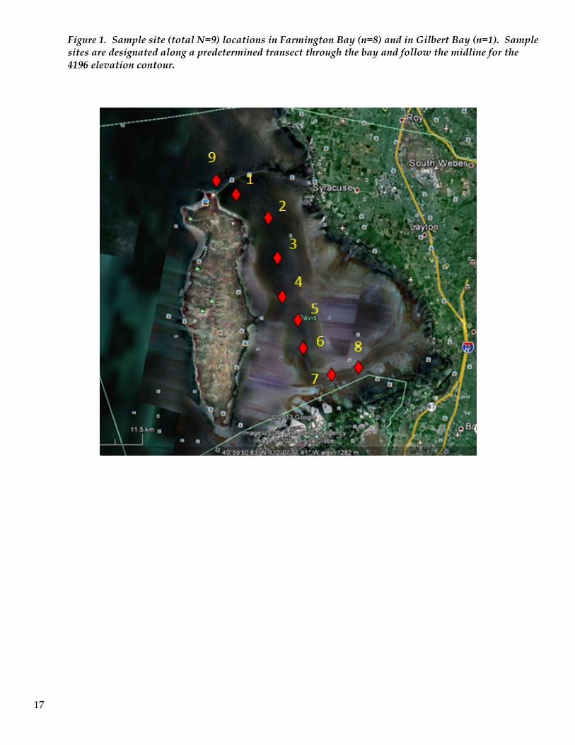
Figure 1. Sample site (total N=9) locations in Farmington Bay (n=8) and in Gilbert Bay (n=1). Sample sites are designated along a predetermined transect through the bay and follow the midline for the 4196 elevation contour.
18
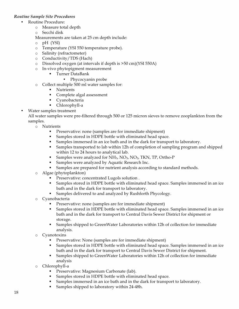
Routine Sample Site Procedures • Routine Procedure:
o Measure total depth o Secchi disk Measurements are taken at 25 cm depth include: o pH (YSI) o Temperature (YSI 550 temperature probe). o Salinity (refractometer) o Conductivity/TDS (Hach) o Dissolved oxygen (at intervals if depth is >50 cm)(YSI 550A) o In-vivo phytopigment measurement
! Turner DataBank • Phycocyanin probe
o Collect multiple 500 ml water samples for: ! Nutrients ! Complete algal assessment ! Cyanobacteria ! Chlorophyll-a
• Water samples treatment All water samples were pre-filtered through 500 or 125 micron sieves to remove zooplankton from the samples.
o Nutrients ! Preservative: none (samples are for immediate shipment) ! Samples stored in HDPE bottle with eliminated head space. ! Samples immersed in an ice bath and in the dark for transport to laboratory. ! Samples transported to lab within 12h of completion of sampling program and shipped
within 12 to 24 hours to analytical lab. ! Samples were analyzed for NH3, NO3, NO2, TKN, TP, Ortho-P ! Samples were analyzed by Aquatic Research Inc. ! Samples are prepared for nutrient analysis according to standard methods.
o Algae (phytoplankton) ! Preservative: concentrated Lugols solution . ! Samples stored in HDPE bottle with eliminated head space. Samples immersed in an ice
bath and in the dark for transport to laboratory. ! Samples delivered to and analyzed by Rushforth Phycology.
o Cyanobacteria ! Preservative: none (samples are for immediate shipment) ! Samples stored in HDPE bottle with eliminated head space. Samples immersed in an ice
bath and in the dark for transport to Central Davis Sewer District for shipment or storage.
! Samples shipped to GreenWater Laboratories within 12h of collection for immediate analysis.
o Cyanotoxins ! Preservative: None (samples are for immediate shipment) ! Samples stored in HDPE bottle with eliminated head space. Samples immersed in an ice
bath and in the dark for transport to Central Davis Sewer District for shipment. ! Samples shipped to GreenWater Laboratories within 12h of collection for immediate
analysis o Chlorophyll-a
! Preservative: Magnesium Carbonate (lab). ! Samples stored in HDPE bottle with eliminated head space. ! Samples immersed in an ice bath and in the dark for transport to laboratory. ! Samples shipped to laboratory within 24-48h.
19
! Samples analyzed by Aquatic Research Inc. • Net haul samples treatment:
o Macroinvertebrates ! Vertical net haul from bottom of water column using a 50 cm diameter plankton net
with 65 micron mesh and affixed with detachable collection cup. ! Entire contents were judiciously washed from net and into receiving collection cup. ! Collection cup contents repeatedly rinsed with filtered Farmington Bay water into 4 liter
sealed container. ! Samples immersed in an ice bath and in the dark for transport to laboratory. ! Zooplankton were then isolated from 4-liter container by filtration through 30 micron
sieve and then rinsed into glass specimen jar. ! Preservative: Buffered Formalin was added to the specimen jar to a final concentration
of 2.5% buffered formaline. ! Samples were then transported to the laboratory of Dr. Lawrence Gray, UVU for
identification and enumeration. ! Sample identification and enumeration was carried out to the species level if possible.
Enumeration includes population age class structure and fecundity assessments. Analytical Methods
Cyanotoxin Measurements and Cyanobacteria Identification and Enumeration (GreenWater Laboratories) Nodularins/Microcystins
! High performance liquid chromatography (HPLC) systems with photodiode array (PDA), fluorescence (FL), and mass spectrometry (MSn) detection.
Cyanobacteria Identification and Enumeration • Samples were preserved with Lugols solution. • Then Utermöhl counting chambers were constructed. Depending on the cell density of
the sample settling towers of 5, 10 or 25 mL were used. Towers were secured to base using a thin film of high vacuum grease. Minimum settling times were 17 hours for 5 mL samples, 34 hrs for 10 mL samples and 74 hours for 25 mL samples.
• Enumerations were performed on a Nikon Eclipse TE200 inverted microscope equipped with phase contrast optics.
• A minimum of 400-600 natural units per slide were counted to give a 95% confidence interval of the estimate within +10% of the sample mean. QA/QC checks were performed at least once for every 10 samples counted and included a check for random distribution of cells (standard error among total number of natural units/field was calculated as the count was being performed with a goal of 15% or less) and a replicate count (goal being a difference between counts of 15% or less). New samples were prepared if samples failed to reach the QA/QC objectives.
Nutrients, Chlorophyll-a, pH, Salinity and Conductivity(Aquatic Research, Inc.)
• Ammonia: Automated Phenate, EPA# 350.1, Standard Method # 4500NH3H • Nitrate/Nitrite: Automated Cadmium Reduction, EPA# 353.2, Standard Method # 4500NO3F • Total Kjeldahl Nitrogen: micro-Kjeldahl, EPA # 351.1, Standard Method #4500NORGC • Total Phosphorous: Automated Ascorbic Acid, EPA# 365.1, Standard Method #4500PF • Soluble Reactive Phosphate: 0.45 micron filtration, EPA # 365.1, Standard Method #4500PF • Salinity: Conductometric, Standard Method # 252OB • pH: Potentiometric, EPA # 150.1, Standard Method #4500H+B • Conductivity: Conductometric, EPA # 120.1, Standard Method #251OB
Analytical Laboratories
20
Nutrients, Chlorophyll-a, pH, Salinity and Conductivity
Aquatic Research, Inc. 3927 Aurora Avenue North Seattle, WA 98103 Phone: 206.632.2715 http://www.aquaticresearchinc.com/contact.html Certifications:
• Washington State Department of Ecology for the analysis of environmental and drinking water samples.
• State of California by the Department of Health Services Environmental Laboratory Accreditation Program (ELAP)
Cyanotoxins and Cyanobacteria Identification
GreenWater Laboratories 205 Zeagler Drive Suite 302 Palatka, FL 32177 Phone: 386.328.0882 http://www.greenwaterlab.com/contactus.html
Phytoplankton Identification Rushforth Phycology 4123 Bona Villa Drive Ogden, UT 84403 801-376-3516 http://rushforthphycology.com/201.html
Zooplankton Identification Dr. Lawrence Gray Department of Biology Utah Valley University 800 W. University Parkway Orem, UT 84058 (801) 863-8558
Phytoplankton Identification and Enumeration
• Samples are filtered through a 1.2 micron pore filter • Cells retained on the filter are resuspended in 5 ml of distilled water • Subsamples are isolated placed in a Palmer Counting Chamber and viewed with a Nikon CF160
Infinity Optical System at 160X to 400X • Identification is carried out to species level of taxa if possible and if species cannot be confirmed
then identification is determined to genus level. • Samples for diatom analysis are separately prepared using nitric acid digestion coupled with
potassium dichromate staining. • Diatoms are then slide mounted and identified using a Nikon Eclipse E200 microscope equipped
with a Nikon CF160 optical system.
21
• Identification is to the lowest taxonomic level possible; species or genus level if possible, otherwise categorized according to centric or pinnate diatoms.
• Biovolume, relative abundance, and rank are determined or calculated along with cell counts. • Detailed SOPs are available from Rushforth Phycology
Zooplankton Identification and Enumeration
• Samples are thoroughly mixed to ensure uniform distribution. • Subsamples are then collected and dispensed into counting cells • All zooplankton contained in subsamples are identified to lowest taxa possible. • Age-class categories are identified, defined and enumerated according to standard procedures and
distinctions. • Gravid females are separately assessed. • Biomass is calculated based on species composition and population size per liter.
Spatial and Seasonal Patterns of the Macroinvertebrate Assemblage in FB
Ordination techniques are often superior to hypothesis testing approaches for explaining relationships
between multivariate ecological assemblages or communities (McCune and Grace 2002). In general,
ordination is the ordering of objects along axes according to their (dis)similarities. The main objective
of ordination is data reduction and expressing many-dimensional relationships into a small number of
easily interpretable dimensions (axes on a plot). The strongest correlation structure in the data is
extracted and is then used to position objects in ordination space. Objects that are close in the
ordination space are generally more similar than objects distant in ordination space (McCune and
Mefford 2011).
Several types of ordination exist; non-metric multidimensional scaling (NMS) was used for this
analysis. NMS has been shown to be robust for ordination of species composition and is often more
useful than other ordination techniques because, among other things, it avoids the assumption of linear
relationships among variables. NMS is also the most widely accepted ordination technique used in
community ecology (Peck 2010). NMS ordination permitted the visualization of the multidimensional
relationships of the macroinvertebrate assemblages in our FBay dataset into a more easily visualized
lower dimensional space. Dimensional reduction obviously creates some distortion in relationships
between samples. The level of reduction in distortion is measured as ‘stress’; less stress equals less
distortion.
Dry weight biomass (micrograms) of macroinvertebrate taxa were estimated from the literature and
then calculated from the density (number/L) values in the data. Biomass data were then log
generalized transformed prior to NMS analyses using PC-ORD (2011)(Version 6.0). Taxa biomasses
22
were log generalized transformed1 to dampen the influence of highly abundant taxa (e.g. Tricocorixid
taxa) and to balance assemblage relationships with rare and uncommon taxa that occurred at low
abundances (Gauch 1982; Efron and Tibshirani 1991; Cao et al. 1998). Taxa with ≤ 2 occurrences in the
sixty- eight samples were also removed from the analyses, which resulted in nine taxa used in the final
analyses. A Sorensen (Bray-Curtis) distance measure was used in the NMS analysis and run for 250
iterations using the real data and 250 iterations in randomized Monte Carlo simulations. The Sorensen
distance measure is based on pairwise comparisons between all sample pairs, therefore NMS
ordinations were rotated using varimax rotation to maximize variation along the axes, and extracted as
univariate scores. Because standardized log-abundance variables are approximately normally
distributed, axes are a linear combination of these variables, and are approximately normally
distributed as well.
The best model was chosen based on scree plots and final significant stress values. Centroid labels
were added to the ordination plots to better interpret the spatial and temporal macroinvertebrate
assemblage relationships. Post- hoc proportion of variance represented by each axis was calculated
based on the R2 value between distance in the ordination space and distance in the original space.
Individual macroinvertebrate taxa correlations with NMS axes were also calculated and those with
strong correlations (r > 0.50) were added to the plots. Graphs of the relative proportion of the nine taxa
per sample in ordination space were also made. Correlations between salinity and NMS axes were also
made. Missing salinity measurements (N = 12) were averaged per site before correlating with NMS
axes.
Macroinvertebrate Assemblages relationships to environmental variables
MRPP (multi-response permutation procedure), a non-parametric method, was also used to formally
test the null hypothesis of no spatial and temporal differences in macroinvertebrate assemblage groups.
MRPP has the advantage of not requiring distributional assumptions such as multivariate normality
and homogeneity of variance and is often superior to MANOVA (McCune and Grace 2002). As is
NMS, MRPP is one of the more useful ordination methods for analyzing multivariate ecological data.
A Euclidean distance measure was used in this MRPP analysis. The chance-corrected within-group test
statistic, A (and associated p-value) was used to evaluate the hypothesis of no difference in the
groupings (McCune and Grace 2002).
Food web analysis
1 See Appendix 1 for description of log generalized transformations
23
Structural Equation Modeling (SEM) methods
Structural Equation modeling, SEM is a combination of a large number of statistical models used to
evaluate the validity of proposed relationships using empirical data and is related to path analysis.
Statistically, SEM represents an extension of general linear modeling (GLM) procedures, such as
ANOVA and multiple regression analysis (Acock 2013). One of the primary advantages of SEM (vs.
other applications of GLM) is that it can be used to study the relationships among latent constructs that
are indicated by multiple measures. SEM typically takes a confirmatory (hypothesis testing) approach
to the multivariate analysis. The causal pattern is specified a priori. The goal is to determine whether a
hypothesized theoretical model is consistent with the data collected. The consistency is evaluated
through model-data fit, which indicates the extent to which the postulated network of relations among
variables is plausible (Acock 2013). SEM is a large sample technique (usually N > 200) and the sample
size required is somewhat dependent on model complexity, the estimation method used, and the
distributional characteristics of observed variables.
We used SEM based on our limited data more as an exploratory but somewhat confirmatory model to
help us construct cursory food web models. We used maximum likelihood with missing values with a
maximum of 200 iterations using the SEM package in STATA 13. We did not evaluate or validate the
model further because we only wanted to begin exploration of the paths between variables and to help
us to understand the food web dynamics and to construct more realistic models after we collect and
assimilate additional data. We attempted to link the top down effects of phytoplankton (measured as
non- cyano cells and PTox cells)(primary producers) on nutrients (measured as SRP and TIN) in our
first model but we did not have enough data points and a viable model could not be generated
(remember in SEM models the more links and complex a model is the more data points are necessary)
We then created an SEM with only bottom up effects of nutrients on phytoplankton, top down and
bottom up effects between phytoplankton (primary producers) and zooplankton (primary consumers),
and top down and bottom up effects between zooplankton and corixids (secondary consumers).
The food web model thus constructed has some limited interpretive value for the initial research
results, but it provides an excellent framework for identifying data gaps, causal relationships and
interactions, and for revising experimental design for subsequent field research as well as devising and
implementing mesocosms or complimentary laboratory projects to further determine causal
relationships, interactions, and relevant linkages among and within trophic levels of the food web.
24
RESULTS Abiotic Characteristics Salinity and Conductivity
Salinity varied both spatially and temporally across Farmington Bay throughout the course of the study
period. Salinity was highest in the sites located in the northern region of the bay demonstrating influence
from bidirectional flow of water from Gilbert Bay into Farmington Bay. Within each sample period this
north-south spatial gradient was observed (Figure 2).
25
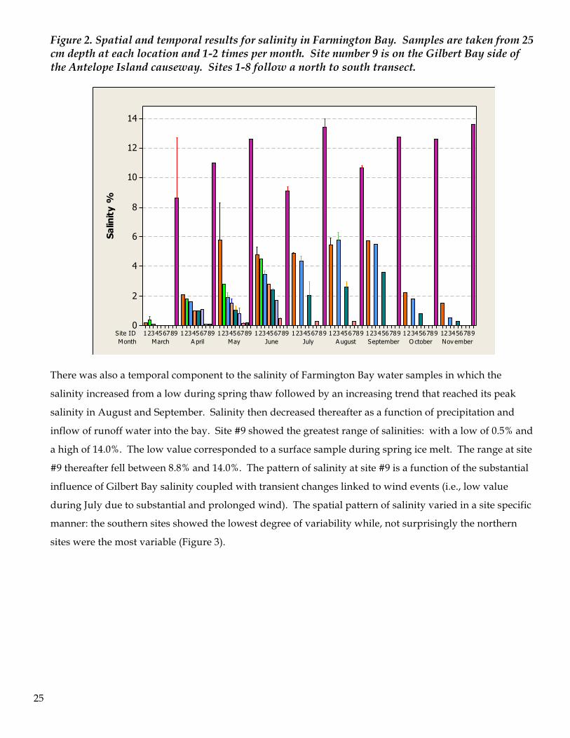
Figure 2. Spatial and temporal results for salinity in Farmington Bay. Samples are taken from 25 cm depth at each location and 1-2 times per month. Site number 9 is on the Gilbert Bay side of the Antelope Island causeway. Sites 1-8 follow a north to south transect.
There was also a temporal component to the salinity of Farmington Bay water samples in which the
salinity increased from a low during spring thaw followed by an increasing trend that reached its peak
salinity in August and September. Salinity then decreased thereafter as a function of precipitation and
inflow of runoff water into the bay. Site #9 showed the greatest range of salinities: with a low of 0.5% and
a high of 14.0%. The low value corresponded to a surface sample during spring ice melt. The range at site
#9 thereafter fell between 8.8% and 14.0%. The pattern of salinity at site #9 is a function of the substantial
influence of Gilbert Bay salinity coupled with transient changes linked to wind events (i.e., low value
during July due to substantial and prolonged wind). The spatial pattern of salinity varied in a site specific
manner: the southern sites showed the lowest degree of variability while, not surprisingly the northern
sites were the most variable (Figure 3).
MonthSite ID
Nov emberO ctoberSeptemberA ugustJulyJuneMayA prilMarch987654321987654321987654321987654321987654321987654321987654321987654321987654321
14
12
10
8
6
4
2
0
Salin
ity
%
26
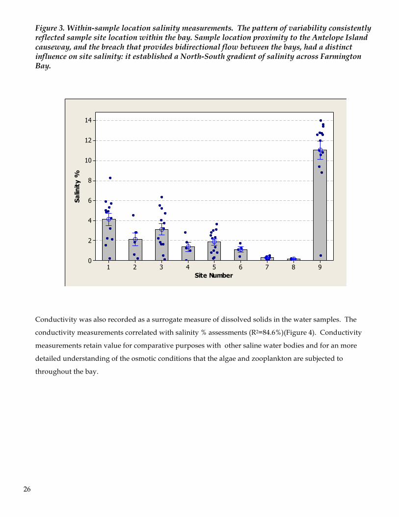
Figure 3. Within-sample location salinity measurements. The pattern of variability consistently reflected sample site location within the bay. Sample location proximity to the Antelope Island causeway, and the breach that provides bidirectional flow between the bays, had a distinct influence on site salinity: it established a North-South gradient of salinity across Farmington Bay.
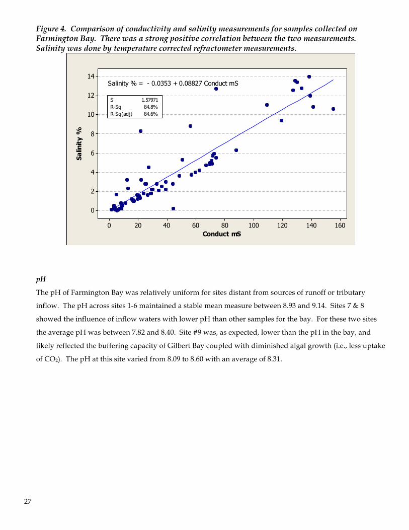
Conductivity was also recorded as a surrogate measure of dissolved solids in the water samples. The
conductivity measurements correlated with salinity % assessments (R2=84.6%)(Figure 4). Conductivity
measurements retain value for comparative purposes with other saline water bodies and for an more
detailed understanding of the osmotic conditions that the algae and zooplankton are subjected to
throughout the bay.
987654321
14
12
10
8
6
4
2
0
Site Number
Salin
ity
%
27
Figure 4. Comparison of conductivity and salinity measurements for samples collected on Farmington Bay. There was a strong positive correlation between the two measurements. Salinity was done by temperature corrected refractometer measurements.
pH
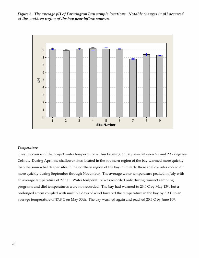
The pH of Farmington Bay was relatively uniform for sites distant from sources of runoff or tributary
inflow. The pH across sites 1-6 maintained a stable mean measure between 8.93 and 9.14. Sites 7 & 8
showed the influence of inflow waters with lower pH than other samples for the bay. For these two sites
the average pH was between 7.82 and 8.40. Site #9 was, as expected, lower than the pH in the bay, and
likely reflected the buffering capacity of Gilbert Bay coupled with diminished algal growth (i.e., less uptake
of CO2). The pH at this site varied from 8.09 to 8.60 with an average of 8.31.
160140120100806040200
14
12
10
8
6
4
2
0
Conduct mS
Salin
ity
%
S 1.57971R-Sq 84.8%R-Sq(adj) 84.6%
Salinity % = - 0.0353 + 0.08827 Conduct mS
28
Figure 5. The average pH of Farmington Bay sample locations. Notable changes in pH occurred at the southern region of the bay near inflow sources.
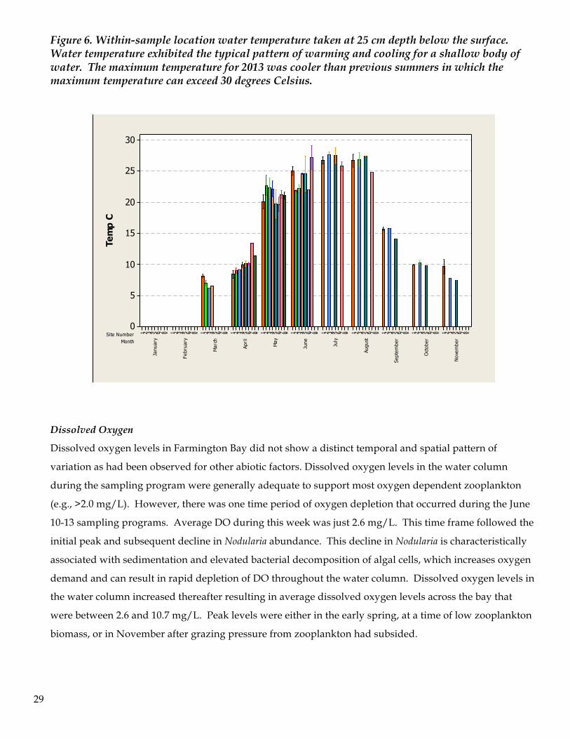
Temperature
Over the course of the project water temperature within Farmington Bay was between 6.2 and 29.2 degrees
Celsius. During April the shallower sites located in the southern region of the bay warmed more quickly
than the somewhat deeper sites in the northern region of the bay. Similarly these shallow sites cooled off
more quickly during September through November. The average water temperature peaked in July with
an average temperature of 27.5 C. Water temperature was recorded only during transect sampling
programs and diel temperatures were not recorded. The bay had warmed to 23.0 C by May 13th, but a
prolonged storm coupled with multiple days of wind lowered the temperature in the bay by 5.3 C to an
average temperature of 17.8 C on May 30th. The bay warmed again and reached 25.3 C by June 10th.
987654321
9
8
7
6
5
4
3
2
1
0
Site Number
pH
29
Figure 6. Within-sample location water temperature taken at 25 cm depth below the surface. Water temperature exhibited the typical pattern of warming and cooling for a shallow body of water. The maximum temperature for 2013 was cooler than previous summers in which the maximum temperature can exceed 30 degrees Celsius.
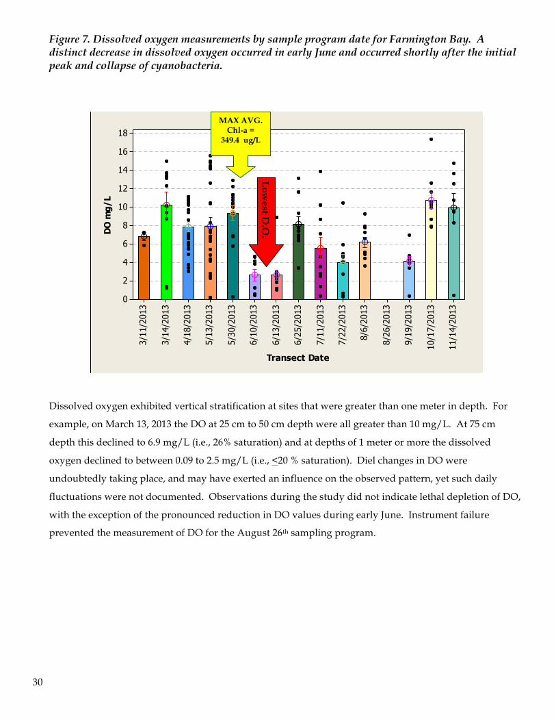
Dissolved Oxygen
Dissolved oxygen levels in Farmington Bay did not show a distinct temporal and spatial pattern of
variation as had been observed for other abiotic factors. Dissolved oxygen levels in the water column
during the sampling program were generally adequate to support most oxygen dependent zooplankton
(e.g., >2.0 mg/L). However, there was one time period of oxygen depletion that occurred during the June
10-13 sampling programs. Average DO during this week was just 2.6 mg/L. This time frame followed the
initial peak and subsequent decline in Nodularia abundance. This decline in Nodularia is characteristically
associated with sedimentation and elevated bacterial decomposition of algal cells, which increases oxygen
demand and can result in rapid depletion of DO throughout the water column. Dissolved oxygen levels in
the water column increased thereafter resulting in average dissolved oxygen levels across the bay that
were between 2.6 and 10.7 mg/L. Peak levels were either in the early spring, at a time of low zooplankton
biomass, or in November after grazing pressure from zooplankton had subsided.
MonthSite Number
Nov
embe
r
Oct
ober
Sept
embe
r
Augu
st
July
JuneMay
Apri
l
Mar
ch
Febr
uary
Janu
ary
*87654321*87654321*87654321*87654321*87654321*87654321*87654321*87654321*87654321*87654321*8765432130
25
20
15
10
5
0
Tem
p C
30
Figure 7. Dissolved oxygen measurements by sample program date for Farmington Bay. A distinct decrease in dissolved oxygen occurred in early June and occurred shortly after the initial peak and collapse of cyanobacteria.
Dissolved oxygen exhibited vertical stratification at sites that were greater than one meter in depth. For
example, on March 13, 2013 the DO at 25 cm to 50 cm depth were all greater than 10 mg/L. At 75 cm
depth this declined to 6.9 mg/L (i.e., 26% saturation) and at depths of 1 meter or more the dissolved
oxygen declined to between 0.09 to 2.5 mg/L (i.e., <20 % saturation). Diel changes in DO were
undoubtedly taking place, and may have exerted an influence on the observed pattern, yet such daily
fluctuations were not documented. Observations during the study did not indicate lethal depletion of DO,
with the exception of the pronounced reduction in DO values during early June. Instrument failure
prevented the measurement of DO for the August 26th sampling program.
11/14/2013
10/17/2013
9/19/2013
8/26/2013
8/6/2013
7/22/2013
7/11/2013
6/25/2013
6/13/2013
6/10/2013
5/30/2013
5/13/2013
4/18/2013
3/14/2013
3/11/2013
18
16
14
12
10
8
6
4
2
0
Transect Date
DO
mg/
LMAX AVG.
Chl-a = 349.4 ug/L
Low
est D.O
.
31
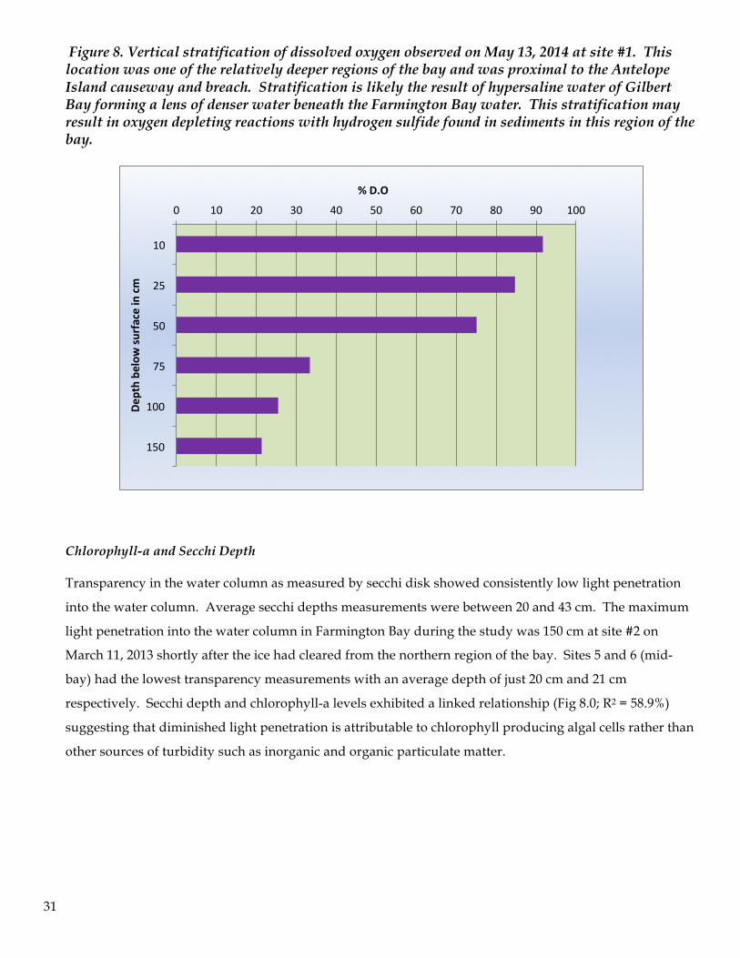
Figure 8. Vertical stratification of dissolved oxygen observed on May 13, 2014 at site #1. This location was one of the relatively deeper regions of the bay and was proximal to the Antelope Island causeway and breach. Stratification is likely the result of hypersaline water of Gilbert Bay forming a lens of denser water beneath the Farmington Bay water. This stratification may result in oxygen depleting reactions with hydrogen sulfide found in sediments in this region of the bay.
Chlorophyll-a and Secchi Depth Transparency in the water column as measured by secchi disk showed consistently low light penetration
into the water column. Average secchi depths measurements were between 20 and 43 cm. The maximum
light penetration into the water column in Farmington Bay during the study was 150 cm at site #2 on
March 11, 2013 shortly after the ice had cleared from the northern region of the bay. Sites 5 and 6 (mid-
bay) had the lowest transparency measurements with an average depth of just 20 cm and 21 cm
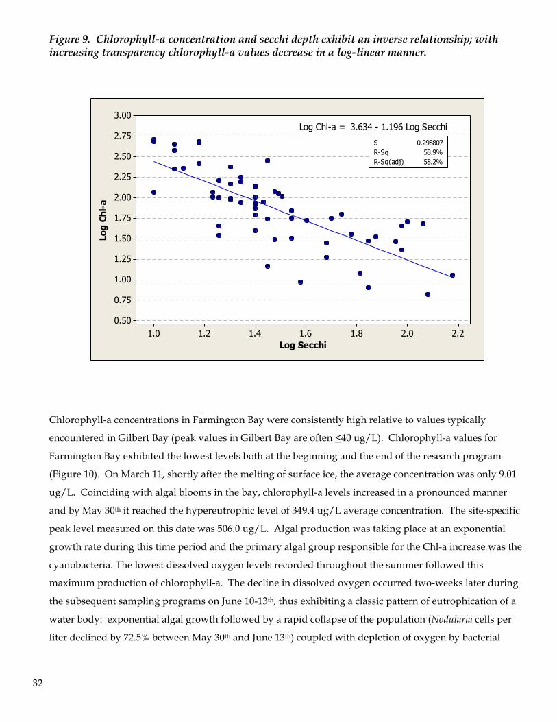
respectively. Secchi depth and chlorophyll-a levels exhibited a linked relationship (Fig 8.0; R2 = 58.9%)
suggesting that diminished light penetration is attributable to chlorophyll producing algal cells rather than
other sources of turbidity such as inorganic and organic particulate matter.
0 10 20 30 40 50 60 70 80 90 100
10
25
50
75
100
150
% D.O
Depth be
low su
rface in cm
32
Figure 9. Chlorophyll-a concentration and secchi depth exhibit an inverse relationship; with increasing transparency chlorophyll-a values decrease in a log-linear manner.
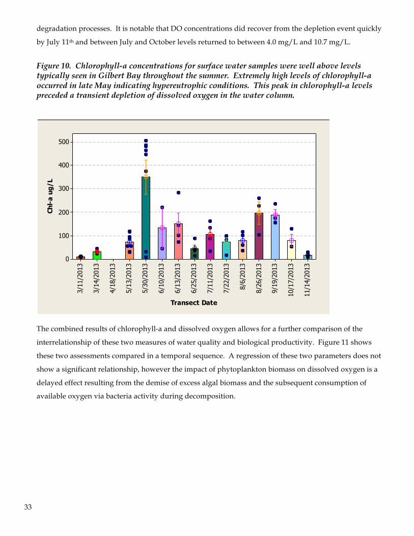
Chlorophyll-a concentrations in Farmington Bay were consistently high relative to values typically
encountered in Gilbert Bay (peak values in Gilbert Bay are often <40 ug/L). Chlorophyll-a values for
Farmington Bay exhibited the lowest levels both at the beginning and the end of the research program
(Figure 10). On March 11, shortly after the melting of surface ice, the average concentration was only 9.01
ug/L. Coinciding with algal blooms in the bay, chlorophyll-a levels increased in a pronounced manner
and by May 30th it reached the hypereutrophic level of 349.4 ug/L average concentration. The site-specific
peak level measured on this date was 506.0 ug/L. Algal production was taking place at an exponential
growth rate during this time period and the primary algal group responsible for the Chl-a increase was the
cyanobacteria. The lowest dissolved oxygen levels recorded throughout the summer followed this
maximum production of chlorophyll-a. The decline in dissolved oxygen occurred two-weeks later during
the subsequent sampling programs on June 10-13th, thus exhibiting a classic pattern of eutrophication of a
water body: exponential algal growth followed by a rapid collapse of the population (Nodularia cells per
liter declined by 72.5% between May 30th and June 13th) coupled with depletion of oxygen by bacterial
2.22.01.81.61.41.21.0
3.00
2.75
2.50
2.25
2.00
1.75
1.50
1.25
1.00
0.75
0.50
Log Secchi
Log
Chl-
a
S 0.298807R-Sq 58.9%R-Sq(adj) 58.2%
Log Chl-a = 3.634 - 1.196 Log Secchi
33
degradation processes. It is notable that DO concentrations did recover from the depletion event quickly
by July 11th and between July and October levels returned to between 4.0 mg/L and 10.7 mg/L.
Figure 10. Chlorophyll-a concentrations for surface water samples were well above levels typically seen in Gilbert Bay throughout the summer. Extremely high levels of chlorophyll-a occurred in late May indicating hypereutrophic conditions. This peak in chlorophyll-a levels preceded a transient depletion of dissolved oxygen in the water column.
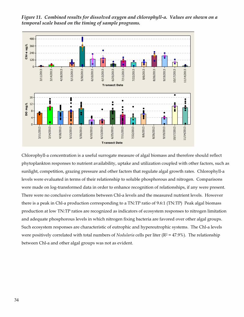
The combined results of chlorophyll-a and dissolved oxygen allows for a further comparison of the
interrelationship of these two measures of water quality and biological productivity. Figure 11 shows
these two assessments compared in a temporal sequence. A regression of these two parameters does not
show a significant relationship, however the impact of phytoplankton biomass on dissolved oxygen is a
delayed effect resulting from the demise of excess algal biomass and the subsequent consumption of
available oxygen via bacteria activity during decomposition.
11/14/2013
10/17/2013
9/19/2013
8/26/2013
8/6/2013
7/22/2013
7/11/2013
6/25/2013
6/13/2013
6/10/2013
5/30/2013
5/13/2013
4/18/2013
3/14/2013
3/11/2013
500
400
300
200
100
0
Transect Date
Chl-
a ug
/L
34
Figure 11. Combined results for dissolved oxygen and chlorophyll-a. Values are shown on a temporal scale based on the timing of sample programs.
Chlorophyll-a concentration is a useful surrogate measure of algal biomass and therefore should reflect
phytoplankton responses to nutrient availability, uptake and utilization coupled with other factors, such as
sunlight, competition, grazing pressure and other factors that regulate algal growth rates. Chlorophyll-a
levels were evaluated in terms of their relationship to soluble phosphorous and nitrogen. Comparisons
were made on log-transformed data in order to enhance recognition of relationships, if any were present.
There were no conclusive correlations between Chl-a levels and the measured nutrient levels. However
there is a peak in Chl-a production corresponding to a TN:TP ratio of 9.6:1 (TN:TP) Peak algal biomass
production at low TN:TP ratios are recognized as indicators of ecosystem responses to nitrogen limitation
and adequate phosphorous levels in which nitrogen fixing bacteria are favored over other algal groups.
Such ecosystem responses are characteristic of eutrophic and hypereutrophic systems. The Chl-a levels
were positively correlated with total numbers of Nodularia cells per liter (R2 = 47.9%). The relationship
between Chl-a and other algal groups was not as evident.
11/14/2013
10/17/2013
9/19/2013
8/26/2013
8/6/2013
7/22/2013
7/11/2013
6/25/2013
6/13/2013
6/10/2013
5/30/2013
5/13/2013
4/18/2013
3/14/2013
3/11/2013
480
360
240
120
0
T ransect Date
Ch
l-a
ug
/L
11/14/2013
10/17/2013
9/19/2013
8/26/2013
8/6/2013
7/22/2013
7/11/2013
6/25/2013
6/13/2013
6/10/2013
5/30/2013
5/13/2013
4/18/2013
3/14/2013
3/11/2013
16
12
8
4
0
T ransect Date
DO
mg
/L
35
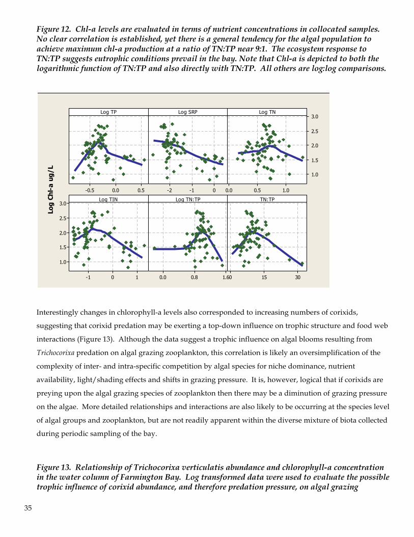
Figure 12. Chl-a levels are evaluated in terms of nutrient concentrations in collocated samples. No clear correlation is established, yet there is a general tendency for the algal population to achieve maximum chl-a production at a ratio of TN:TP near 9:1. The ecosystem response to TN:TP suggests eutrophic conditions prevail in the bay. Note that Chl-a is depicted to both the logarithmic function of TN:TP and also directly with TN:TP. All others are log:log comparisons.
Interestingly changes in chlorophyll-a levels also corresponded to increasing numbers of corixids,
suggesting that corixid predation may be exerting a top-down influence on trophic structure and food web
interactions (Figure 13). Although the data suggest a trophic influence on algal blooms resulting from
Trichocorixa predation on algal grazing zooplankton, this correlation is likely an oversimplification of the
complexity of inter- and intra-specific competition by algal species for niche dominance, nutrient
availability, light/shading effects and shifts in grazing pressure. It is, however, logical that if corixids are
preying upon the algal grazing species of zooplankton then there may be a diminution of grazing pressure
on the algae. More detailed relationships and interactions are also likely to be occurring at the species level
of algal groups and zooplankton, but are not readily apparent within the diverse mixture of biota collected
during periodic sampling of the bay.
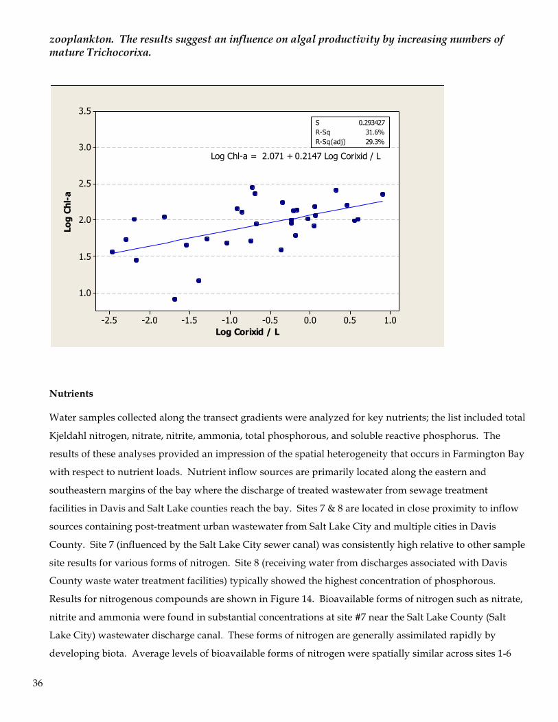
Figure 13. Relationship of Trichocorixa verticulatis abundance and chlorophyll-a concentration in the water column of Farmington Bay. Log transformed data were used to evaluate the possible trophic influence of corixid abundance, and therefore predation pressure, on algal grazing
0.50.0-0.5 0-1-2 1.00.50.0
3.0
2.5
2.0
1.5
1.0
10-1
3.0
2.5
2.0
1.5
1.0
1.60.80.0 30150
Log TP
Log
Chl-
a ug
/L
Log SRP Log TN
Log TIN Log TN:TP TN:TP
36
zooplankton. The results suggest an influence on algal productivity by increasing numbers of mature Trichocorixa.
Nutrients Water samples collected along the transect gradients were analyzed for key nutrients; the list included total
Kjeldahl nitrogen, nitrate, nitrite, ammonia, total phosphorous, and soluble reactive phosphorus. The
results of these analyses provided an impression of the spatial heterogeneity that occurs in Farmington Bay
with respect to nutrient loads. Nutrient inflow sources are primarily located along the eastern and
southeastern margins of the bay where the discharge of treated wastewater from sewage treatment
facilities in Davis and Salt Lake counties reach the bay. Sites 7 & 8 are located in close proximity to inflow
sources containing post-treatment urban wastewater from Salt Lake City and multiple cities in Davis
County. Site 7 (influenced by the Salt Lake City sewer canal) was consistently high relative to other sample
site results for various forms of nitrogen. Site 8 (receiving water from discharges associated with Davis
County waste water treatment facilities) typically showed the highest concentration of phosphorous.
Results for nitrogenous compounds are shown in Figure 14. Bioavailable forms of nitrogen such as nitrate,
nitrite and ammonia were found in substantial concentrations at site #7 near the Salt Lake County (Salt
Lake City) wastewater discharge canal. These forms of nitrogen are generally assimilated rapidly by
developing biota. Average levels of bioavailable forms of nitrogen were spatially similar across sites 1-6
1.00.50.0-0.5-1.0-1.5-2.0-2.5
3.5
3.0
2.5
2.0
1.5
1.0
Log Corixid / L
Log
Chl-
a
S 0.293427R-Sq 31.6%R-Sq(adj) 29.3%
Log Chl-a = 2.071 + 0.2147 Log Corixid / L
37
when evaluated over the full time frame of the ice-free time period on Farmington Bay. The nitrate &
nitrite concentration was between 0.01 and 6.57 mg/L with a collective average of 0.52 mg/L. Ammonia
fell between 0.01 and 16.29 mg/L and exhibited an overall average of 0.65 mg/L. If we omit the high
concentration associated with site #7 the upper limit for nitrate & nitrite is 2.26 mg/L and for ammonia it is
3.01 mg/L. The organic fraction of nitrogen expressed as total Kjeldahl nitrogen (TKN) fell between 1.35
mg/L and 19.33 mg/L (again at site #7). Without inclusion of site #7 the upper limit was 10.55 mg/L at
site #1. The TKN average was 4.06 mg/L. Total nitrogen had a lower limit of 1.44 mg/L and an upper
value of 19.82 mg/L, and excluding site #7 the highest value was 10.57 mg/L. The bay-wide average for
the entire ice-free period for all sites was 4.58 mg/L. This value may be an underestimate of the nitrogen
load in the bay because evaporative loss of volume precluded access to sites 7 & 8 from September to the
end of the study, thereby rendering it impossible to collect samples at the location that had previously
demonstrated the highest values.
38
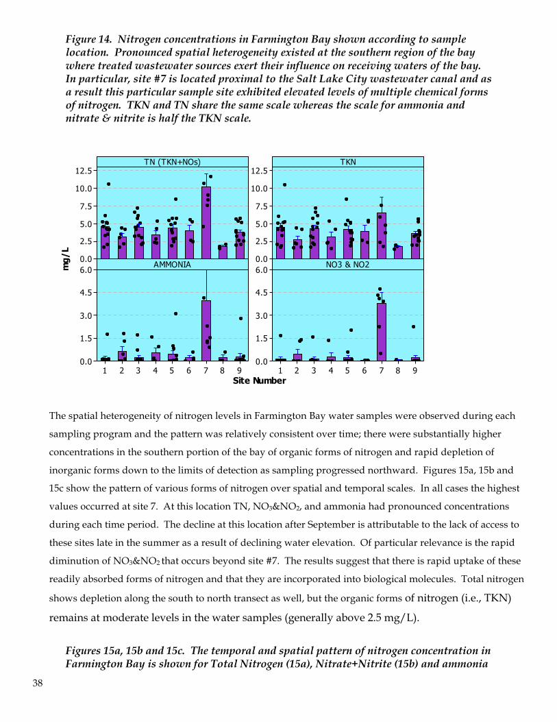
Figure 14. Nitrogen concentrations in Farmington Bay shown according to sample location. Pronounced spatial heterogeneity existed at the southern region of the bay where treated wastewater sources exert their influence on receiving waters of the bay. In particular, site #7 is located proximal to the Salt Lake City wastewater canal and as a result this particular sample site exhibited elevated levels of multiple chemical forms of nitrogen. TKN and TN share the same scale whereas the scale for ammonia and nitrate & nitrite is half the TKN scale.
The spatial heterogeneity of nitrogen levels in Farmington Bay water samples were observed during each
sampling program and the pattern was relatively consistent over time; there were substantially higher
concentrations in the southern portion of the bay of organic forms of nitrogen and rapid depletion of
inorganic forms down to the limits of detection as sampling progressed northward. Figures 15a, 15b and
15c show the pattern of various forms of nitrogen over spatial and temporal scales. In all cases the highest
values occurred at site 7. At this location TN, NO3&NO2, and ammonia had pronounced concentrations
during each time period. The decline at this location after September is attributable to the lack of access to
these sites late in the summer as a result of declining water elevation. Of particular relevance is the rapid
diminution of NO3&NO2 that occurs beyond site #7. The results suggest that there is rapid uptake of these
readily absorbed forms of nitrogen and that they are incorporated into biological molecules. Total nitrogen
shows depletion along the south to north transect as well, but the organic forms of nitrogen (i.e., TKN)
remains at moderate levels in the water samples (generally above 2.5 mg/L).
Figures 15a, 15b and 15c. The temporal and spatial pattern of nitrogen concentration in Farmington Bay is shown for Total Nitrogen (15a), Nitrate+Nitrite (15b) and ammonia
12.5
10.0
7.5
5.0
2.5
0.0
12.5
10.0
7.5
5.0
2.5
0.0
987654321
6.0
4.5
3.0
1.5
0.0987654321
6.0
4.5
3.0
1.5
0.0
TN (TKN+NOs)
Site Number
mg/
L
TKN
AMMONIA NO3 & NO2
39
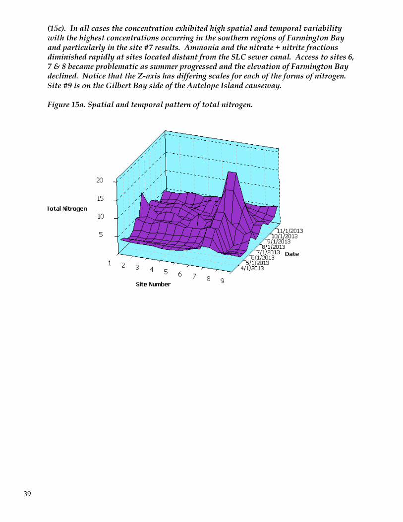
(15c). In all cases the concentration exhibited high spatial and temporal variability with the highest concentrations occurring in the southern regions of Farmington Bay and particularly in the site #7 results. Ammonia and the nitrate + nitrite fractions diminished rapidly at sites located distant from the SLC sewer canal. Access to sites 6, 7 & 8 became problematic as summer progressed and the elevation of Farmington Bay declined. Notice that the Z-axis has differing scales for each of the forms of nitrogen. Site #9 is on the Gilbert Bay side of the Antelope Island causeway.
Figure 15a. Spatial and temporal pattern of total nitrogen.
40
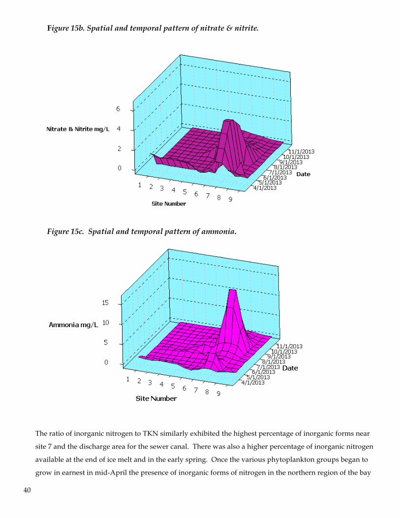
Figure 15b. Spatial and temporal pattern of nitrate & nitrite.
Figure 15c. Spatial and temporal pattern of ammonia.
The ratio of inorganic nitrogen to TKN similarly exhibited the highest percentage of inorganic forms near
site 7 and the discharge area for the sewer canal. There was also a higher percentage of inorganic nitrogen
available at the end of ice melt and in the early spring. Once the various phytoplankton groups began to
grow in earnest in mid-April the presence of inorganic forms of nitrogen in the northern region of the bay
41
remained low indicating rapid uptake and depletion of bioavailable inorganic forms of nitrogen (Figure
16).
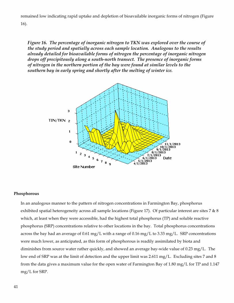
Figure 16. The percentage of inorganic nitrogen to TKN was explored over the course of the study period and spatially across each sample location. Analogous to the results already detailed for bioavailable forms of nitrogen the percentage of inorganic nitrogen drops off precipitously along a south-north transect. The presence of inorganic forms of nitrogen in the northern portion of the bay were found at similar levels to the southern bay in early spring and shortly after the melting of winter ice.
Phosphorous
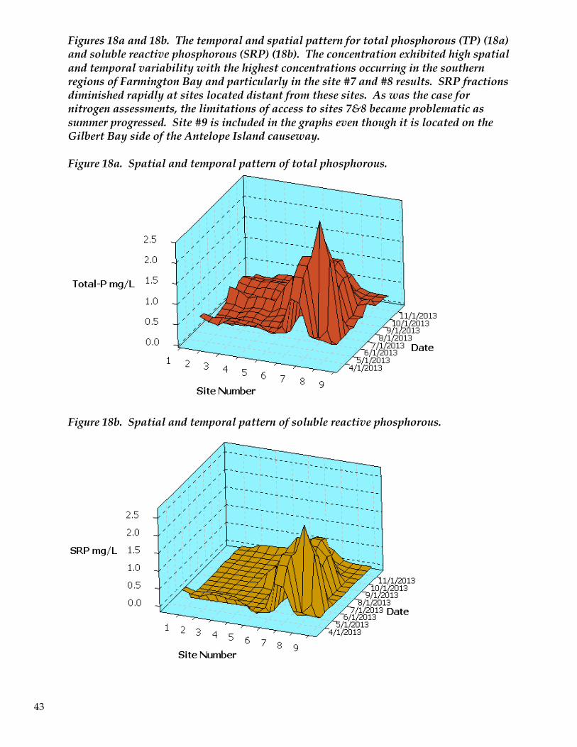
In an analogous manner to the pattern of nitrogen concentrations in Farmington Bay, phosphorus
exhibited spatial heterogeneity across all sample locations (Figure 17). Of particular interest are sites 7 & 8
which, at least when they were accessible, had the highest total phosphorus (TP) and soluble reactive
phosphorus (SRP) concentrations relative to other locations in the bay. Total phosphorus concentrations
across the bay had an average of 0.61 mg/L with a range of 0.16 mg/L to 3.33 mg/L. SRP concentrations
were much lower, as anticipated, as this form of phosphorous is readily assimilated by biota and
diminishes from source water rather quickly, and showed an average bay-wide value of 0.23 mg/L. The
low end of SRP was at the limit of detection and the upper limit was 2.611 mg/L. Excluding sites 7 and 8
from the data gives a maximum value for the open water of Farmington Bay of 1.80 mg/L for TP and 1.147
mg/L for SRP.
42
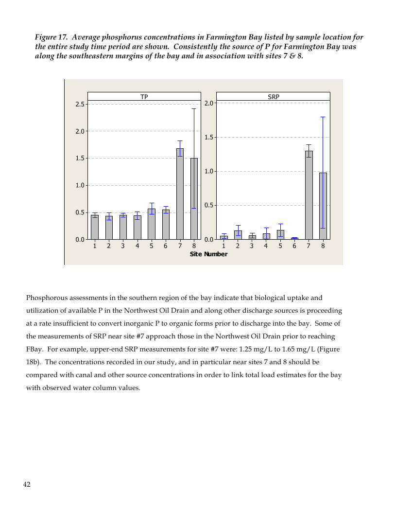
Figure 17. Average phosphorus concentrations in Farmington Bay listed by sample location for the entire study time period are shown. Consistently the source of P for Farmington Bay was along the southeastern margins of the bay and in association with sites 7 & 8.
Phosphorous assessments in the southern region of the bay indicate that biological uptake and
utilization of available P in the Northwest Oil Drain and along other discharge sources is proceeding
at a rate insufficient to convert inorganic P to organic forms prior to discharge into the bay. Some of
the measurements of SRP near site #7 approach those in the Northwest Oil Drain prior to reaching
FBay. For example, upper-end SRP measurements for site #7 were: 1.25 mg/L to 1.65 mg/L (Figure
18b). The concentrations recorded in our study, and in particular near sites 7 and 8 should be
compared with canal and other source concentrations in order to link total load estimates for the bay
with observed water column values.
87654321
2.5
2.0
1.5
1.0
0.5
0.087654321
2.0
1.5
1.0
0.5
0.0
TP
Site Number
SRP
43
Figures 18a and 18b. The temporal and spatial pattern for total phosphorous (TP) (18a) and soluble reactive phosphorous (SRP) (18b). The concentration exhibited high spatial and temporal variability with the highest concentrations occurring in the southern regions of Farmington Bay and particularly in the site #7 and #8 results. SRP fractions diminished rapidly at sites located distant from these sites. As was the case for nitrogen assessments, the limitations of access to sites 7&8 became problematic as summer progressed. Site #9 is included in the graphs even though it is located on the Gilbert Bay side of the Antelope Island causeway.
Figure 18a. Spatial and temporal pattern of total phosphorous.
Figure 18b. Spatial and temporal pattern of soluble reactive phosphorous.
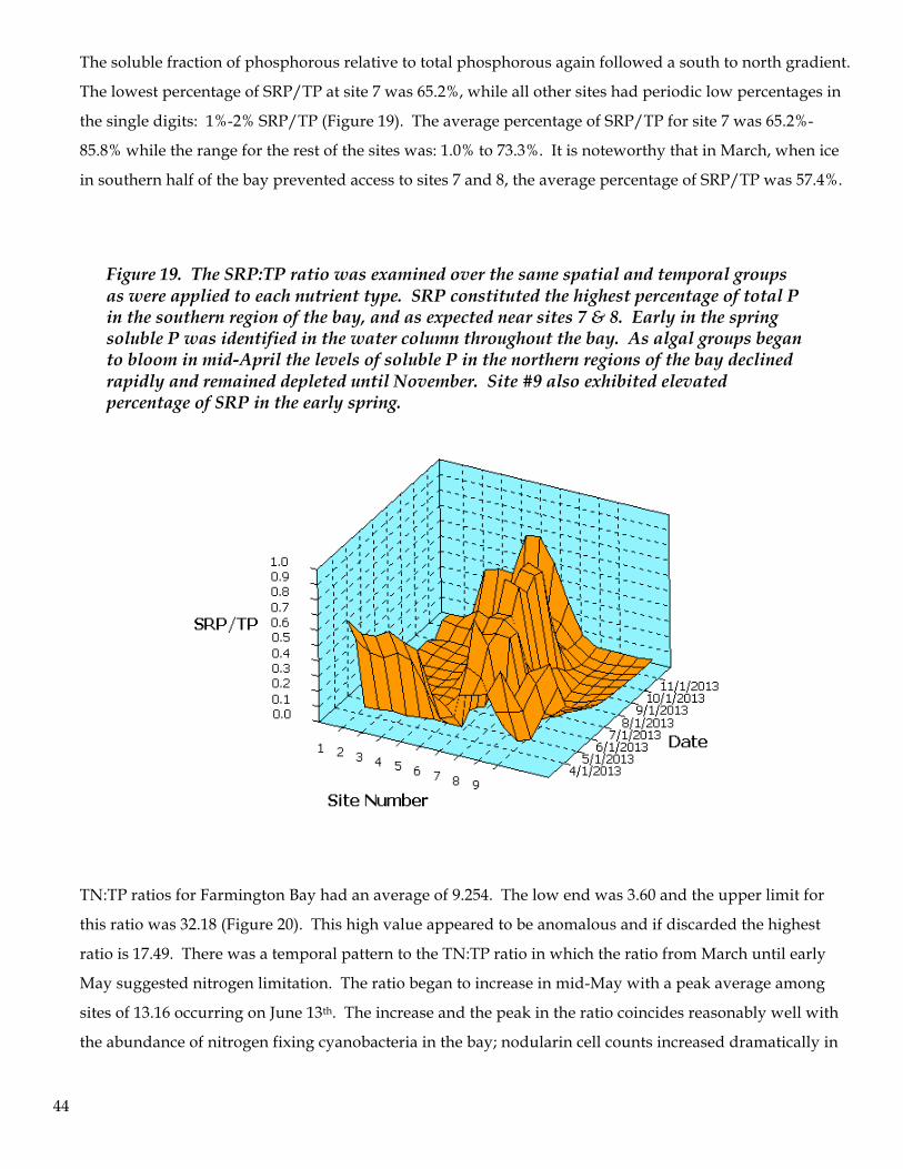
44
The soluble fraction of phosphorous relative to total phosphorous again followed a south to north gradient.
The lowest percentage of SRP/TP at site 7 was 65.2%, while all other sites had periodic low percentages in
the single digits: 1%-2% SRP/TP (Figure 19). The average percentage of SRP/TP for site 7 was 65.2%-
85.8% while the range for the rest of the sites was: 1.0% to 73.3%. It is noteworthy that in March, when ice
in southern half of the bay prevented access to sites 7 and 8, the average percentage of SRP/TP was 57.4%.
Figure 19. The SRP:TP ratio was examined over the same spatial and temporal groups as were applied to each nutrient type. SRP constituted the highest percentage of total P in the southern region of the bay, and as expected near sites 7 & 8. Early in the spring soluble P was identified in the water column throughout the bay. As algal groups began to bloom in mid-April the levels of soluble P in the northern regions of the bay declined rapidly and remained depleted until November. Site #9 also exhibited elevated percentage of SRP in the early spring.
TN:TP ratios for Farmington Bay had an average of 9.254. The low end was 3.60 and the upper limit for
this ratio was 32.18 (Figure 20). This high value appeared to be anomalous and if discarded the highest
ratio is 17.49. There was a temporal pattern to the TN:TP ratio in which the ratio from March until early
May suggested nitrogen limitation. The ratio began to increase in mid-May with a peak average among
sites of 13.16 occurring on June 13th. The increase and the peak in the ratio coincides reasonably well with
the abundance of nitrogen fixing cyanobacteria in the bay; nodularin cell counts increased dramatically in
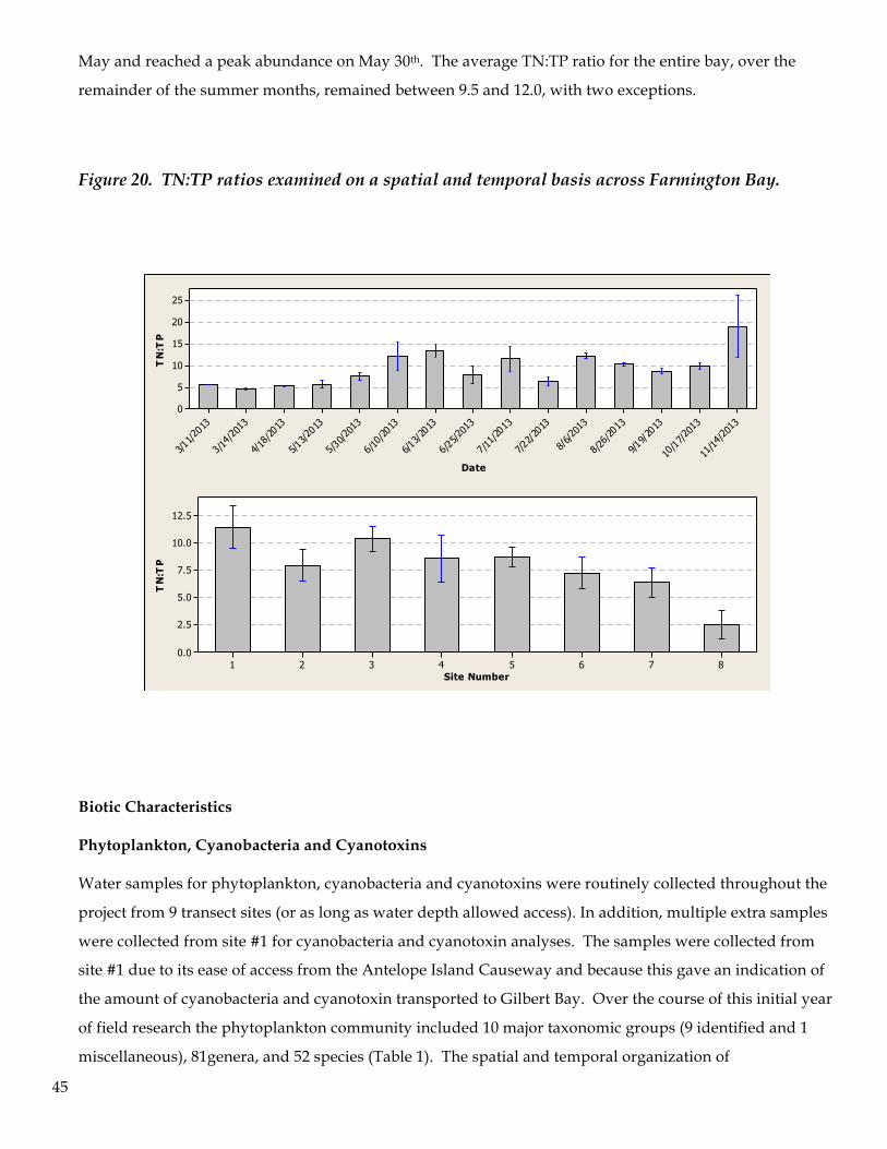
45
May and reached a peak abundance on May 30th. The average TN:TP ratio for the entire bay, over the
remainder of the summer months, remained between 9.5 and 12.0, with two exceptions.
Figure 20. TN:TP ratios examined on a spatial and temporal basis across Farmington Bay.
Biotic Characteristics Phytoplankton, Cyanobacteria and Cyanotoxins Water samples for phytoplankton, cyanobacteria and cyanotoxins were routinely collected throughout the
project from 9 transect sites (or as long as water depth allowed access). In addition, multiple extra samples
were collected from site #1 for cyanobacteria and cyanotoxin analyses. The samples were collected from
site #1 due to its ease of access from the Antelope Island Causeway and because this gave an indication of
the amount of cyanobacteria and cyanotoxin transported to Gilbert Bay. Over the course of this initial year
of field research the phytoplankton community included 10 major taxonomic groups (9 identified and 1
miscellaneous), 81genera, and 52 species (Table 1). The spatial and temporal organization of
11/14/2013
10/17/2013
9/19/2013
8/26/2013
8/6/2013
7/22/2013
7/11/2013
6/25/2013
6/13/2013
6/10/2013
5/30/2013
5/13/2013
4/18/2013
3/14/2013
3/11/2013
25
20
15
10
5
0
Date
TN
:TP
87654321
12.5
10.0
7.5
5.0
2.5
0.0
Site Number
TN
:TP
46
phytoplankton in Farmington Bay was in continuous flux; with shifting patterns of abundance attributable
to niche dominance strategies, interspecific competitive displacements, grazing depletion, exponential
growth and dramatic collapse. We also observed the appearance of an asymmetric relationship between
Nodularia abundance and nodularin toxin production indicative of a critical density dependent threshold.
Microalgal assemblages in the bay exhibited a most remarkable array of diversity and shifting dynamics.
Trophic regime changes were observed throughout the observation period and unique site specific as well
as bay-wide patterns of algal dominance and genera specific collapse were documented. To capture the
full scope of the biological diversity and the complexity of the interactions between and within trophic
levels it is necessary to scrutinize site specific changes and to then evaluate those local shifts in diversity
and abundance with respect to the broader developing pattern that emerges when analyzing the bay as a
single limnological entity.
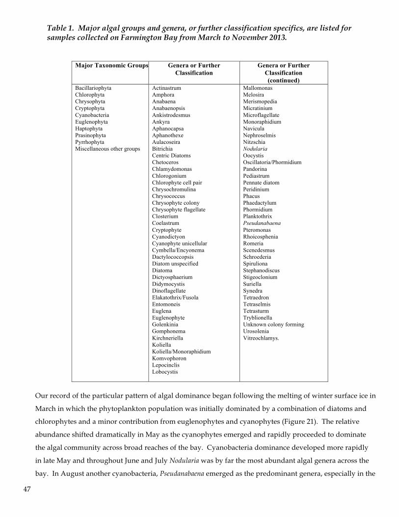
47
Table 1. Major algal groups and genera, or further classification specifics, are listed for samples collected on Farmington Bay from March to November 2013.
Major Taxonomic Groups Genera or Further
Classification
Genera or Further Classification (continued)
Bacillariophyta Chlorophyta Chrysophyta Cryptophyta Cyanobacteria Euglenophyta Haptophyta Prasinophyta Pyrrhophyta Miscellaneous other groups
Actinastrum Amphora Anabaena Anabaenopsis Ankistrodesmus Ankyra Aphanocapsa Aphanothexe Aulacoseira Bitrichia Centric Diatoms Chetoceros Chlamydomonas Chlorogonium Chlorophyte cell pair Chrysochromulina Chrysococcus Chrysophyte colony Chrysophyte flagellate Closterium Coelastrum Cryptophyte Cyanodictyon Cyanophyte unicellular Cymbella/Encyonema Dactylococcopsis Diatom unspecified Diatoma Dictyosphaerium Didymocystis Dinoflagellate Elakatothrix/Fusola Entomoneis Euglena Euglenophyte Golenkinia Gomphonema Kirchneriella Koliella Koliella/Monoraphidium Komvophoron Lepocinclis Lobocystis
Mallomonas Melosira Merismopedia Micratinium Microflagellate Monoraphidium Navicula Nephroselmis Nitzschia Nodularia Oocystis Oscillatoria/Phormidium Pandorina Pediastrum Pennate diatom Peridinium Phacus Phaedactylum Phormidium Planktothrix Pseudanabaena Pteromonas Rhoicosphenia Romeria Scenedesmus Schroederia Spiruliona Stephanodiscus Stigeoclonium Suriella Synedra Tetraedron Tetraselmis Tetrasturm Tryblionella Unknown colony forming Urosolenia Vitreochlamys.
Our record of the particular pattern of algal dominance began following the melting of winter surface ice in
March in which the phytoplankton population was initially dominated by a combination of diatoms and
chlorophytes and a minor contribution from euglenophytes and cyanophytes (Figure 21). The relative
abundance shifted dramatically in May as the cyanophytes emerged and rapidly proceeded to dominate
the algal community across broad reaches of the bay. Cyanobacteria dominance developed more rapidly
in late May and throughout June and July Nodularia was by far the most abundant algal genera across the
bay. In August another cyanobacteria, Pseudanabaena emerged as the predominant genera, especially in the
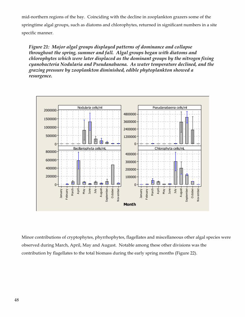
48
mid-northern regions of the bay. Coinciding with the decline in zooplankton grazers some of the
springtime algal groups, such as diatoms and chlorophytes, returned in significant numbers in a site
specific manner.
Figure 21: Major algal groups displayed patterns of dominance and collapse throughout the spring, summer and fall. Algal groups began with diatoms and chlorophytes which were later displaced as the dominant groups by the nitrogen fixing cyanobacteria Nodularia and Pseudanabaena. As water temperature declined, and the grazing pressure by zooplankton diminished, edible phytoplankton showed a resurgence.
Minor contributions of cryptophytes, phyrrhophytes, flagellates and miscellaneous other algal species were
observed during March, April, May and August. Notable among these other divisions was the
contribution by flagellates to the total biomass during the early spring months (Figure 22).
2000000
1500000
1000000
500000
0
4800000
3600000
2400000
1200000
0
Nov
embe
r
Oct
ober
Sep
tem
ber
Aug
ust
July
June
May
Apr
il
Mar
ch
Feb
ruar
y
Janu
ary
800000
600000
400000
200000
0
Nov
embe
r
Oct
ober
Sep
tem
ber
Aug
ust
July
June
May
Apr
il
Mar
ch
Feb
ruar
y
Janu
ary
400000
300000
200000
100000
0
Nodularia cells/ml
Month
Pseudanabaena cells/ml
Bacillariophyta cells/mL Chlorophyta cells/mL
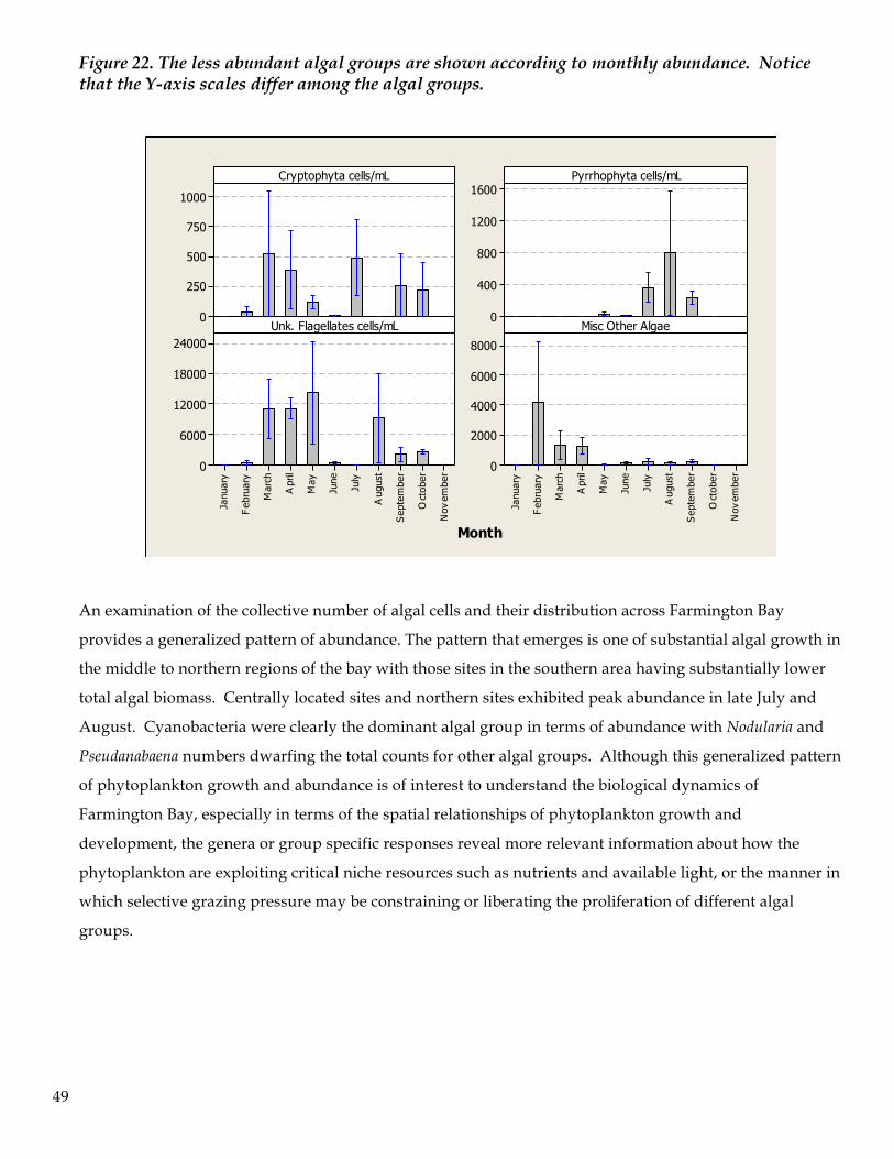
49
Figure 22. The less abundant algal groups are shown according to monthly abundance. Notice that the Y-axis scales differ among the algal groups.
An examination of the collective number of algal cells and their distribution across Farmington Bay
provides a generalized pattern of abundance. The pattern that emerges is one of substantial algal growth in
the middle to northern regions of the bay with those sites in the southern area having substantially lower
total algal biomass. Centrally located sites and northern sites exhibited peak abundance in late July and
August. Cyanobacteria were clearly the dominant algal group in terms of abundance with Nodularia and
Pseudanabaena numbers dwarfing the total counts for other algal groups. Although this generalized pattern
of phytoplankton growth and abundance is of interest to understand the biological dynamics of
Farmington Bay, especially in terms of the spatial relationships of phytoplankton growth and
development, the genera or group specific responses reveal more relevant information about how the
phytoplankton are exploiting critical niche resources such as nutrients and available light, or the manner in
which selective grazing pressure may be constraining or liberating the proliferation of different algal
groups.
1000
750
500
250
0
1600
1200
800
400
0
Nov
embe
r
Oct
ober
Sep
tem
ber
Aug
ust
July
June
May
Apr
il
Mar
ch
Feb
ruar
y
Janu
ary
24000
18000
12000
6000
0
Nov
embe
r
Oct
ober
Sep
tem
ber
Aug
ust
July
June
May
Apr
il
Mar
ch
Feb
ruar
y
Janu
ary
8000
6000
4000
2000
0
Cryptophyta cells/mL
Month
Pyrrhophyta cells/mL
Unk. Flagellates cells/mL Misc Other Algae
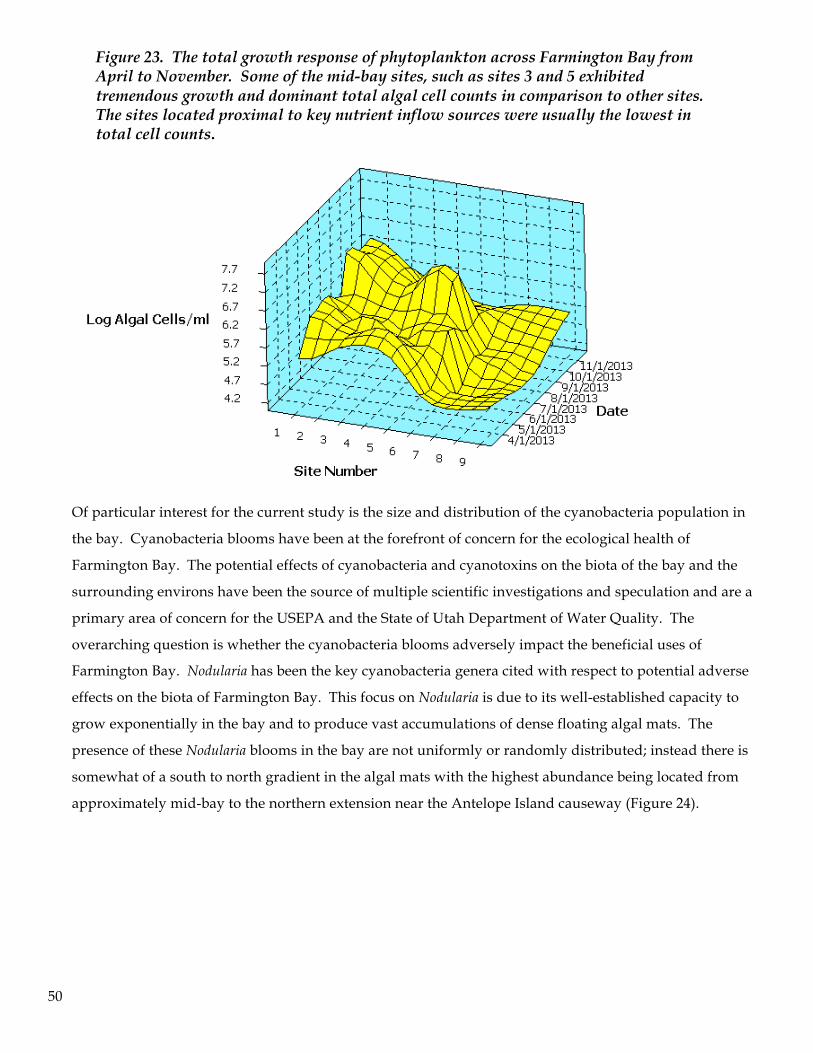
50
Figure 23. The total growth response of phytoplankton across Farmington Bay from April to November. Some of the mid-bay sites, such as sites 3 and 5 exhibited tremendous growth and dominant total algal cell counts in comparison to other sites. The sites located proximal to key nutrient inflow sources were usually the lowest in total cell counts.
Of particular interest for the current study is the size and distribution of the cyanobacteria population in
the bay. Cyanobacteria blooms have been at the forefront of concern for the ecological health of
Farmington Bay. The potential effects of cyanobacteria and cyanotoxins on the biota of the bay and the
surrounding environs have been the source of multiple scientific investigations and speculation and are a
primary area of concern for the USEPA and the State of Utah Department of Water Quality. The
overarching question is whether the cyanobacteria blooms adversely impact the beneficial uses of
Farmington Bay. Nodularia has been the key cyanobacteria genera cited with respect to potential adverse
effects on the biota of Farmington Bay. This focus on Nodularia is due to its well-established capacity to
grow exponentially in the bay and to produce vast accumulations of dense floating algal mats. The
presence of these Nodularia blooms in the bay are not uniformly or randomly distributed; instead there is
somewhat of a south to north gradient in the algal mats with the highest abundance being located from
approximately mid-bay to the northern extension near the Antelope Island causeway (Figure 24).
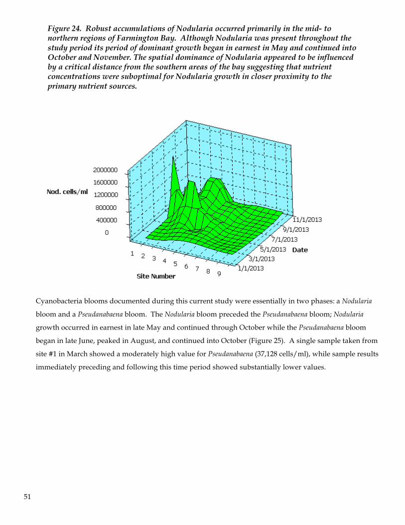
51
Figure 24. Robust accumulations of Nodularia occurred primarily in the mid- to northern regions of Farmington Bay. Although Nodularia was present throughout the study period its period of dominant growth began in earnest in May and continued into October and November. The spatial dominance of Nodularia appeared to be influenced by a critical distance from the southern areas of the bay suggesting that nutrient concentrations were suboptimal for Nodularia growth in closer proximity to the primary nutrient sources.
Cyanobacteria blooms documented during this current study were essentially in two phases: a Nodularia
bloom and a Pseudanabaena bloom. The Nodularia bloom preceded the Pseudanabaena bloom; Nodularia
growth occurred in earnest in late May and continued through October while the Pseudanabaena bloom
began in late June, peaked in August, and continued into October (Figure 25). A single sample taken from
site #1 in March showed a moderately high value for Pseudanabaena (37,128 cells/ml), while sample results
immediately preceding and following this time period showed substantially lower values.
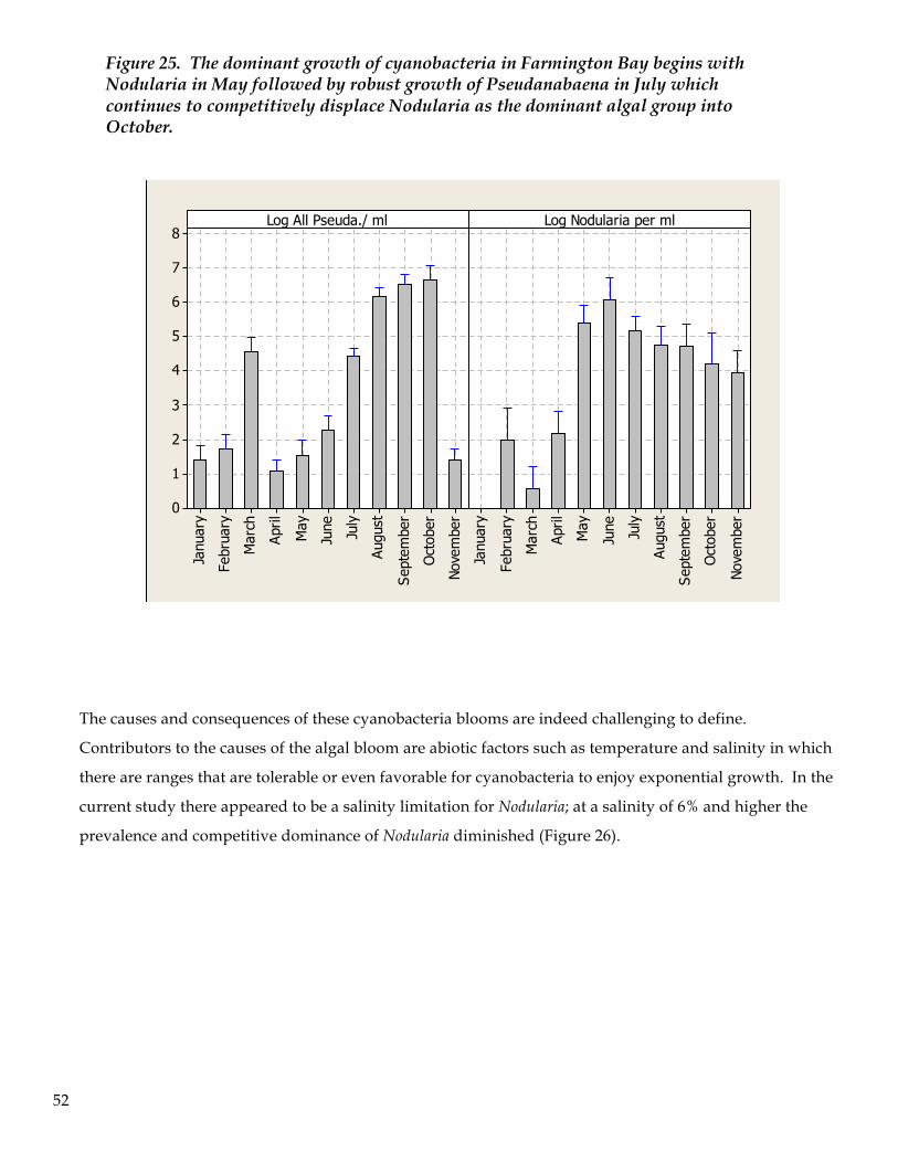
52
Figure 25. The dominant growth of cyanobacteria in Farmington Bay begins with Nodularia in May followed by robust growth of Pseudanabaena in July which continues to competitively displace Nodularia as the dominant algal group into October.
The causes and consequences of these cyanobacteria blooms are indeed challenging to define.
Contributors to the causes of the algal bloom are abiotic factors such as temperature and salinity in which
there are ranges that are tolerable or even favorable for cyanobacteria to enjoy exponential growth. In the
current study there appeared to be a salinity limitation for Nodularia; at a salinity of 6% and higher the
prevalence and competitive dominance of Nodularia diminished (Figure 26).
Nove
mbe
r
Oct
ober
Sept
embe
r
Augu
st
July
June
May
April
Mar
ch
Febr
uary
Janu
ary
8
7
6
5
4
3
2
1
0
Nove
mbe
r
Oct
ober
Sept
embe
r
Augu
st
July
June
May
April
Mar
ch
Febr
uary
Janu
ary
Log All Pseuda./ ml Log Nodularia per ml
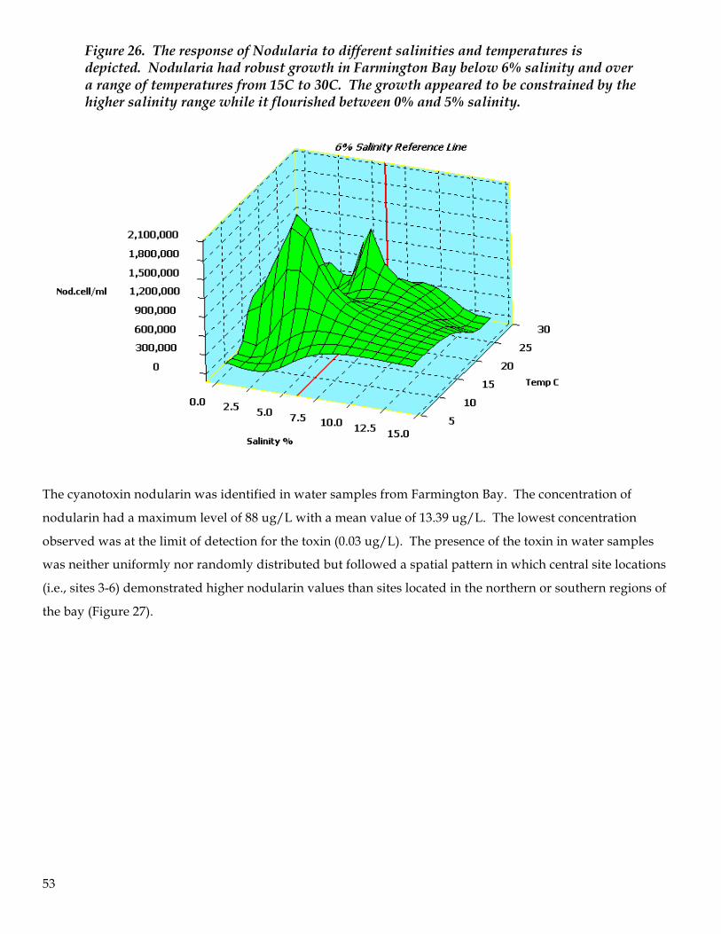
53
Figure 26. The response of Nodularia to different salinities and temperatures is depicted. Nodularia had robust growth in Farmington Bay below 6% salinity and over a range of temperatures from 15C to 30C. The growth appeared to be constrained by the higher salinity range while it flourished between 0% and 5% salinity.
The cyanotoxin nodularin was identified in water samples from Farmington Bay. The concentration of
nodularin had a maximum level of 88 ug/L with a mean value of 13.39 ug/L. The lowest concentration
observed was at the limit of detection for the toxin (0.03 ug/L). The presence of the toxin in water samples
was neither uniformly nor randomly distributed but followed a spatial pattern in which central site locations
(i.e., sites 3-6) demonstrated higher nodularin values than sites located in the northern or southern regions of
the bay (Figure 27).
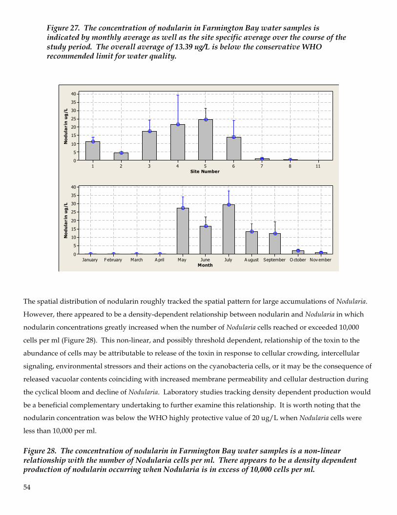
54
Figure 27. The concentration of nodularin in Farmington Bay water samples is indicated by monthly average as well as the site specific average over the course of the study period. The overall average of 13.39 ug/L is below the conservative WHO recommended limit for water quality.
The spatial distribution of nodularin roughly tracked the spatial pattern for large accumulations of Nodularia.
However, there appeared to be a density-dependent relationship between nodularin and Nodularia in which
nodularin concentrations greatly increased when the number of Nodularia cells reached or exceeded 10,000
cells per ml (Figure 28). This non-linear, and possibly threshold dependent, relationship of the toxin to the
abundance of cells may be attributable to release of the toxin in response to cellular crowding, intercellular
signaling, environmental stressors and their actions on the cyanobacteria cells, or it may be the consequence of
released vacuolar contents coinciding with increased membrane permeability and cellular destruction during
the cyclical bloom and decline of Nodularia. Laboratory studies tracking density dependent production would
be a beneficial complementary undertaking to further examine this relationship. It is worth noting that the
nodularin concentration was below the WHO highly protective value of 20 ug/L when Nodularia cells were
less than 10,000 per ml.
Figure 28. The concentration of nodularin in Farmington Bay water samples is a non-linear relationship with the number of Nodularia cells per ml. There appears to be a density dependent production of nodularin occurring when Nodularia is in excess of 10,000 cells per ml.
1187654321
40
35
30
25
20
15
10
5
0
Site Number
No
du
lari
n u
g/L
Nov emberO ctoberSeptemberA ugustJulyJuneMayA prilMarchFebruaryJanuary
40
35
30
25
20
15
10
5
0
Month
No
du
lari
n u
g/L
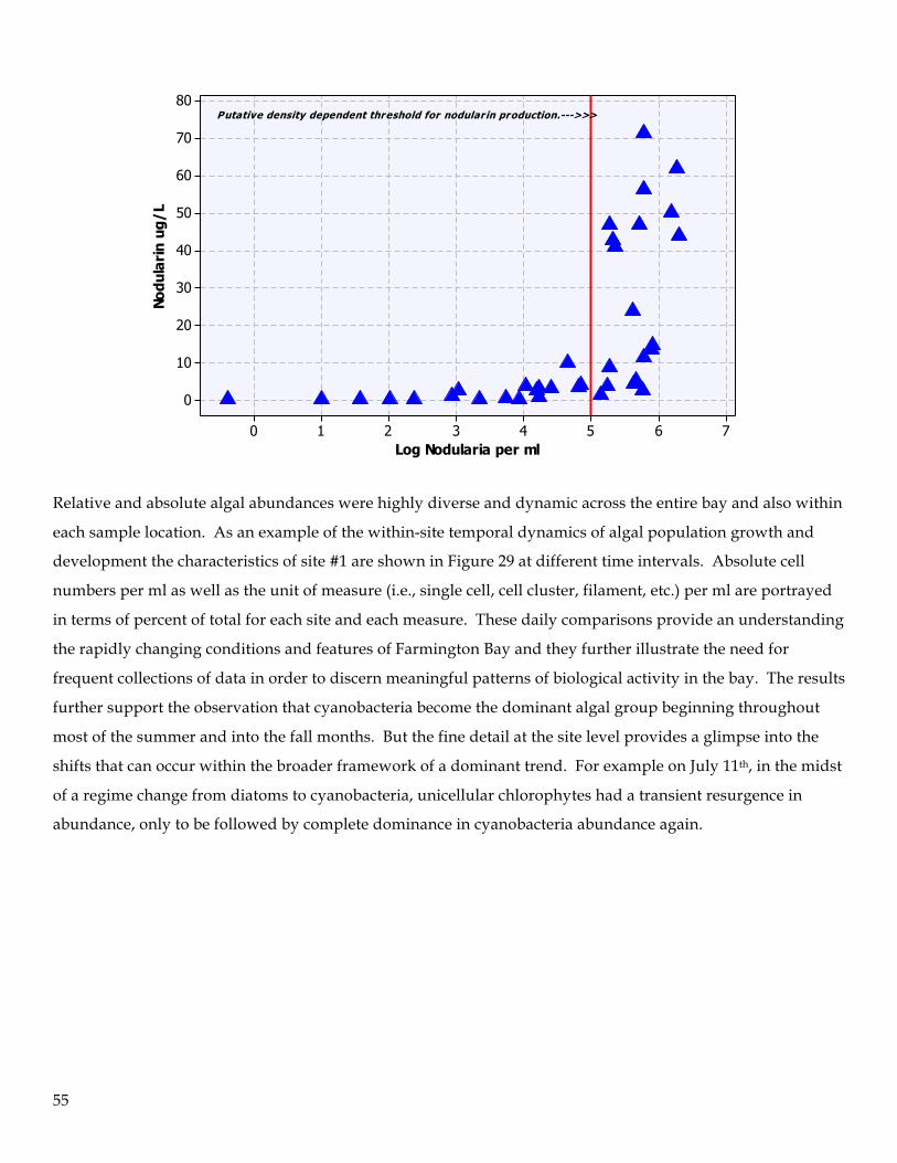
55
Relative and absolute algal abundances were highly diverse and dynamic across the entire bay and also within
each sample location. As an example of the within-site temporal dynamics of algal population growth and
development the characteristics of site #1 are shown in Figure 29 at different time intervals. Absolute cell
numbers per ml as well as the unit of measure (i.e., single cell, cell cluster, filament, etc.) per ml are portrayed
in terms of percent of total for each site and each measure. These daily comparisons provide an understanding
the rapidly changing conditions and features of Farmington Bay and they further illustrate the need for
frequent collections of data in order to discern meaningful patterns of biological activity in the bay. The results
further support the observation that cyanobacteria become the dominant algal group beginning throughout
most of the summer and into the fall months. But the fine detail at the site level provides a glimpse into the
shifts that can occur within the broader framework of a dominant trend. For example on July 11th, in the midst
of a regime change from diatoms to cyanobacteria, unicellular chlorophytes had a transient resurgence in
abundance, only to be followed by complete dominance in cyanobacteria abundance again.
76543210
80
70
60
50
40
30
20
10
0
Log Nodularia per ml
Nodu
lari
n ug
/L
Putative density dependent threshold for nodular in production.--->>>
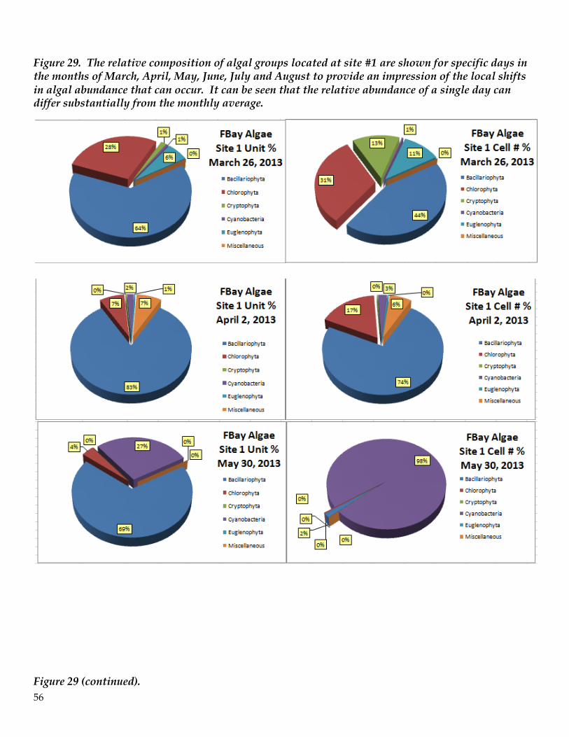
56
Figure 29. The relative composition of algal groups located at site #1 are shown for specific days in the months of March, April, May, June, July and August to provide an impression of the local shifts in algal abundance that can occur. It can be seen that the relative abundance of a single day can differ substantially from the monthly average.
Figure 29 (continued).
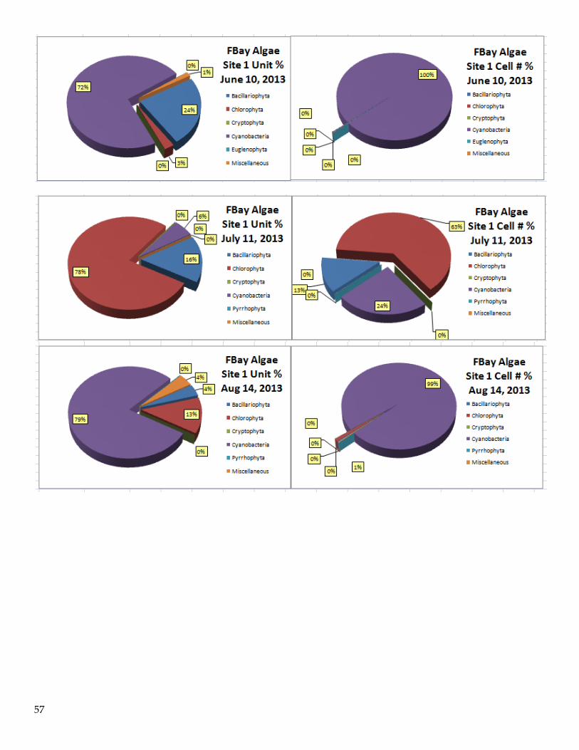
57
58
Zooplankton
A sizeable diversity and remarkable abundance of zooplankton were identified in Farmington Bay. Eight
major groups of zooplankton were observed and included: Cladocera, Copepoda, Branchiopoda, Ostracoda,
Rotifera, Insecta (Diptera and Hemiptera) and Annelida (Oligocheata). Within these taxonomic groups 17
species of zooplankton were found and four unidentified species were consistently observed. All populations
of zooplankton on Farmington Bay exhibited growth and decline patterns throughout the study period.
Additionally, there were spatial differences among the zooplankton likely attributable to salinity tolerance
differences, competition, food availability, predation and other abiotic and biotic factors that exert a
pronounced effect on the distribution of a particular zooplankton species. Within each zooplankton group the
key species in terms of numbers and biomass were: Rotifera—Brachionus plicatilis; Cladocera—Moina
macrocarpa; Copepoda (Harpacticoid)—Cletocamptus sp.; Branchiopoda—Artemia franciscana; Insecta
(Hemiptera)—Trichocorixa verticalis.
Although previous research (Taylor, 2004) has shown the need to use mesh size of less than 100 microns to
collect most microzooplankton it is possible that other microzooplankton, and picozooplankton, such as
protozoans, were not adequately collected nor identified due to the mesh size of the plankton net used for the
current study; the mesh size was 60 microns and the sieve size used to capture the net contents was a 38
micron mesh. Due to these mesh sizes some of the smallest micro- and picoplankton may have been lost in
the sample collection. Additionally, at times of the year when Nodularia blooms were in abundance the
collection and separation of zooplankton from algae became increasingly difficult (selective filtration required
multiple hours per sample) and some loss of the microzooplankton such as rotifers could have occurred.
Zooplankton taxa observed during the study are shown in Table 2. Rotifers and copepods were the most
abundant of the zooplankton observed. Rotifers (Brachionus) exhibited three peak abundances: April, June
and November. The maximum number observed was in June with 1,761 individuals per liter. The copepods
had a maximum abundance of almost twice this level with 3,376 individuals per liter in June. Among the
Rotifera the only species identified in large numbers of substantial biological relevance was Brachionus
plicatilis. One other species (Notholca acuminate) was identified in November 2013 but was insignificant in
abundance (0.13 per liter maximum count). No other species of rotifers were identified in the bay.
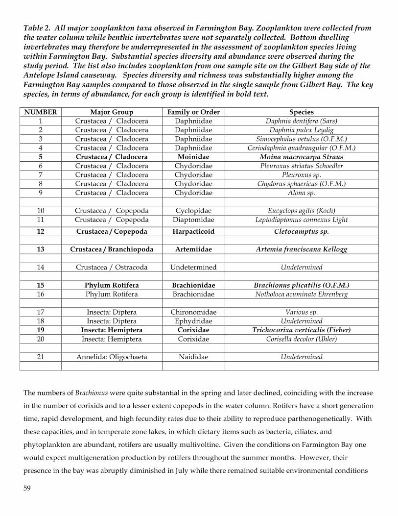
59
Table 2. All major zooplankton taxa observed in Farmington Bay. Zooplankton were collected from the water column while benthic invertebrates were not separately collected. Bottom dwelling invertebrates may therefore be underrepresented in the assessment of zooplankton species living within Farmington Bay. Substantial species diversity and abundance were observed during the study period. The list also includes zooplankton from one sample site on the Gilbert Bay side of the Antelope Island causeway. Species diversity and richness was substantially higher among the Farmington Bay samples compared to those observed in the single sample from Gilbert Bay. The key species, in terms of abundance, for each group is identified in bold text. NUMBER Major Group Family or Order Species
1 Crustacea / Cladocera Daphniidae Daphnia dentifera (Sars) 2 Crustacea / Cladocera Daphniidae Daphnia pulex Leydig 3 Crustacea / Cladocera Daphniidae Simocephalus vetulus (O.F.M.) 4 Crustacea / Cladocera Daphniidae Ceriodaphnia quadrangular (O.F.M.) 5 Crustacea / Cladocera Moinidae Moina macrocarpa Straus 6 Crustacea / Cladocera Chydoridae Pleuroxus striatus Schoedler 7 Crustacea / Cladocera Chydoridae Pleuroxus sp. 8 Crustacea / Cladocera Chydoridae Chydorus sphaericus (O.F.M.) 9 Crustacea / Cladocera Chydoridae Alona sp.
10 Crustacea / Copepoda Cyclopidae Eucyclops agilis (Koch) 11 Crustacea / Copepoda Diaptomidae Leptodiaptomus connexus Light
12 Crustacea / Copepoda Harpacticoid Cletocamptus sp.
13 Crustacea / Branchiopoda Artemiidae Artemia franciscana Kellogg
14 Crustacea / Ostracoda Undetermined Undetermined
15 Phylum Rotifera Brachionidae Brachionus plicatilis (O.F.M.) 16 Phylum Rotifera Brachionidae Notholoca acuminate Ehrenberg
17 Insecta: Diptera Chironomidae Various sp. 18 Insecta: Diptera Ephydridae Undetermined 19 Insecta: Hemiptera Corixidae Trichocorixa verticalis (Fieber) 20 Insecta: Hemiptera Corixidae Corisella decolor (Uhler)
21 Annelida: Oligochaeta Naididae Undetermined
The numbers of Brachionus were quite substantial in the spring and later declined, coinciding with the increase
in the number of corixids and to a lesser extent copepods in the water column. Rotifers have a short generation
time, rapid development, and high fecundity rates due to their ability to reproduce parthenogenetically. With
these capacities, and in temperate zone lakes, in which dietary items such as bacteria, ciliates, and
phytoplankton are abundant, rotifers are usually multivoltine. Given the conditions on Farmington Bay one
would expect multigeneration production by rotifers throughout the summer months. However, their
presence in the bay was abruptly diminished in July while there remained suitable environmental conditions
60
and adequate dietary items for further reproductive output. This abbreviation in reproduction suggests a
“top-down” control by a dominant predator or from multiple predators.
Among the zooplankton, the rotifers were the only taxa that showed a rebound of population numbers in the
late summer and early fall (Figure 30). This rebound in rotifer numbers may reflect renewed favorable
conditions in the bay, hatching of viable and non-resting eggs, or it may be indicative of diminished predation
pressure thus allowing the rotifers to survive and replenish the population. The return of rotifers in the water
column occurred once Corixidae numbers were in substantial decline.
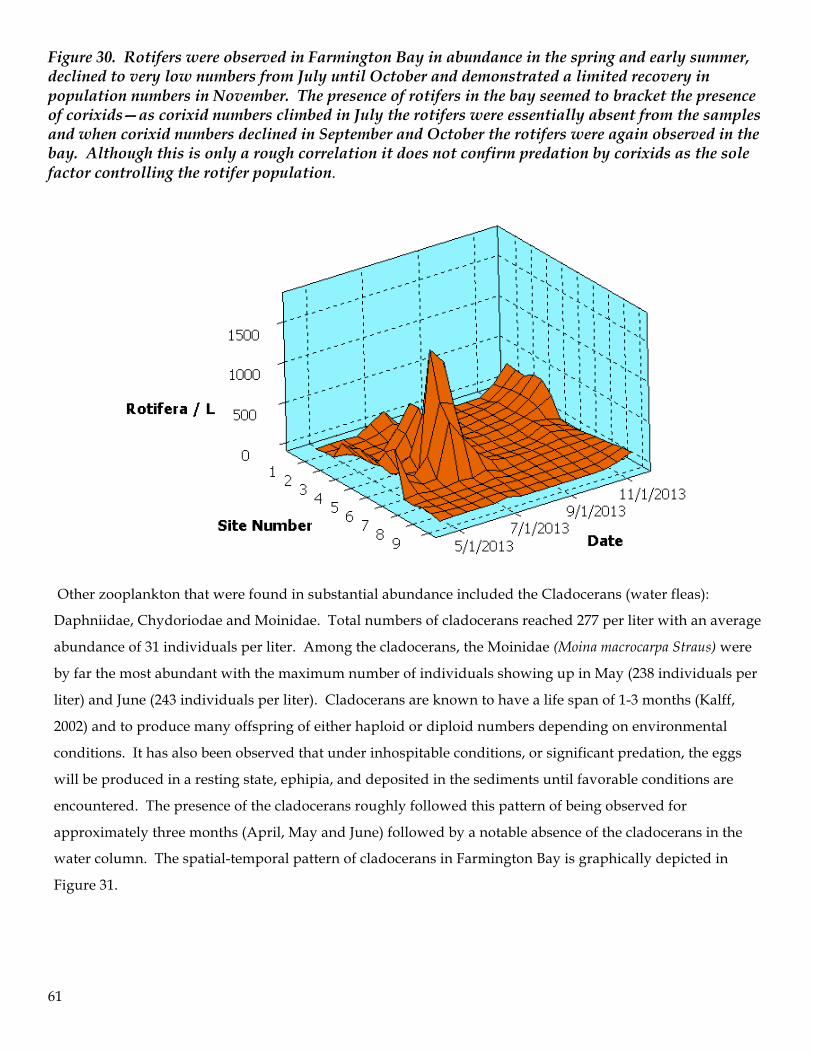
61
Figure 30. Rotifers were observed in Farmington Bay in abundance in the spring and early summer, declined to very low numbers from July until October and demonstrated a limited recovery in population numbers in November. The presence of rotifers in the bay seemed to bracket the presence of corixids—as corixid numbers climbed in July the rotifers were essentially absent from the samples and when corixid numbers declined in September and October the rotifers were again observed in the bay. Although this is only a rough correlation it does not confirm predation by corixids as the sole factor controlling the rotifer population.
Other zooplankton that were found in substantial abundance included the Cladocerans (water fleas):
Daphniidae, Chydoriodae and Moinidae. Total numbers of cladocerans reached 277 per liter with an average
abundance of 31 individuals per liter. Among the cladocerans, the Moinidae (Moina macrocarpa Straus) were
by far the most abundant with the maximum number of individuals showing up in May (238 individuals per
liter) and June (243 individuals per liter). Cladocerans are known to have a life span of 1-3 months (Kalff,
2002) and to produce many offspring of either haploid or diploid numbers depending on environmental
conditions. It has also been observed that under inhospitable conditions, or significant predation, the eggs
will be produced in a resting state, ephipia, and deposited in the sediments until favorable conditions are
encountered. The presence of the cladocerans roughly followed this pattern of being observed for
approximately three months (April, May and June) followed by a notable absence of the cladocerans in the
water column. The spatial-temporal pattern of cladocerans in Farmington Bay is graphically depicted in
Figure 31.
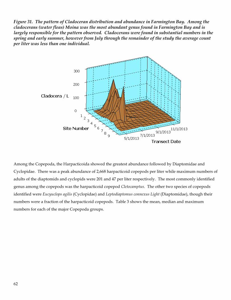
62
Figure 31. The pattern of Cladoceran distribution and abundance in Farmington Bay. Among the cladocerans (water fleas) Moina was the most abundant genus found in Farmington Bay and is largely responsible for the pattern observed. Cladocerans were found in substantial numbers in the spring and early summer, however from July through the remainder of the study the average count per liter was less than one individual.
Among the Copepoda, the Harpacticoida showed the greatest abundance followed by Diaptomidae and
Cyclopidae. There was a peak abundance of 2,668 harpacticoid copepods per liter while maximum numbers of
adults of the diaptomids and cyclopids were 201 and 47 per liter respectively. The most commonly identified
genus among the copepods was the harpacticoid copepod Cletocamptus. The other two species of copepods
identified were Eucyuclops agilis (Cyclopidae) and Leptodiaptomus connexus Light (Diaptomidae), though their
numbers were a fraction of the harpacticoid copepods. Table 3 shows the mean, median and maximum
numbers for each of the major Copepoda groups.
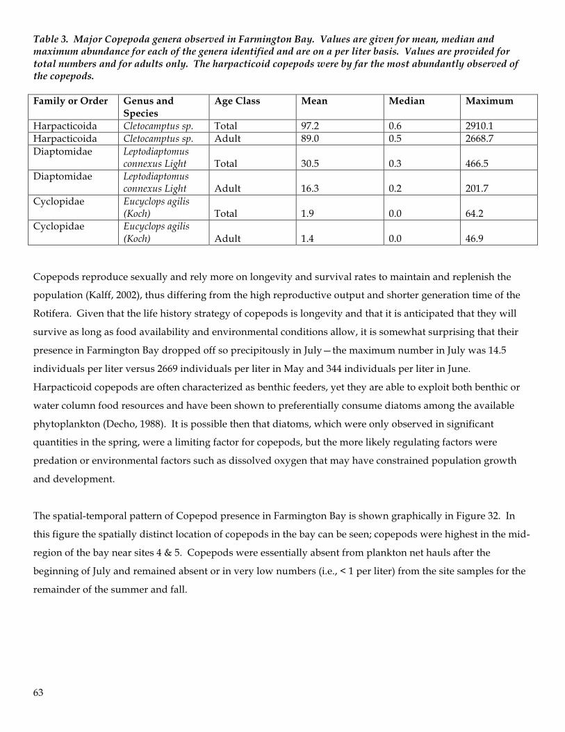
63
Table 3. Major Copepoda genera observed in Farmington Bay. Values are given for mean, median and maximum abundance for each of the genera identified and are on a per liter basis. Values are provided for total numbers and for adults only. The harpacticoid copepods were by far the most abundantly observed of the copepods. Family or Order Genus and
Species Age Class Mean Median Maximum
Harpacticoida Cletocamptus sp. Total 97.2 0.6 2910.1 Harpacticoida Cletocamptus sp. Adult 89.0 0.5 2668.7 Diaptomidae Leptodiaptomus
connexus Light Total
30.5
0.3
466.5
Diaptomidae Leptodiaptomus connexus Light
Adult
16.3
0.2
201.7
Cyclopidae Eucyclops agilis (Koch)
Total
1.9
0.0
64.2
Cyclopidae Eucyclops agilis (Koch)
Adult
1.4
0.0
46.9
Copepods reproduce sexually and rely more on longevity and survival rates to maintain and replenish the
population (Kalff, 2002), thus differing from the high reproductive output and shorter generation time of the
Rotifera. Given that the life history strategy of copepods is longevity and that it is anticipated that they will
survive as long as food availability and environmental conditions allow, it is somewhat surprising that their
presence in Farmington Bay dropped off so precipitously in July—the maximum number in July was 14.5
individuals per liter versus 2669 individuals per liter in May and 344 individuals per liter in June.
Harpacticoid copepods are often characterized as benthic feeders, yet they are able to exploit both benthic or
water column food resources and have been shown to preferentially consume diatoms among the available
phytoplankton (Decho, 1988). It is possible then that diatoms, which were only observed in significant
quantities in the spring, were a limiting factor for copepods, but the more likely regulating factors were
predation or environmental factors such as dissolved oxygen that may have constrained population growth
and development.
The spatial-temporal pattern of Copepod presence in Farmington Bay is shown graphically in Figure 32. In
this figure the spatially distinct location of copepods in the bay can be seen; copepods were highest in the mid-
region of the bay near sites 4 & 5. Copepods were essentially absent from plankton net hauls after the
beginning of July and remained absent or in very low numbers (i.e., < 1 per liter) from the site samples for the
remainder of the summer and fall.
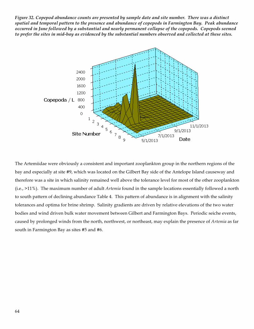
64
Figure 32. Copepod abundance counts are presented by sample date and site number. There was a distinct spatial and temporal pattern to the presence and abundance of copepods in Farmington Bay. Peak abundance occurred in June followed by a substantial and nearly permanent collapse of the copepods. Copepods seemed to prefer the sites in mid-bay as evidenced by the substantial numbers observed and collected at these sites.
The Artemiidae were obviously a consistent and important zooplankton group in the northern regions of the
bay and especially at site #9, which was located on the Gilbert Bay side of the Antelope Island causeway and
therefore was a site in which salinity remained well above the tolerance level for most of the other zooplankton
(i.e., >11%). The maximum number of adult Artemia found in the sample locations essentially followed a north
to south pattern of declining abundance Table 4. This pattern of abundance is in alignment with the salinity
tolerances and optima for brine shrimp. Salinity gradients are driven by relative elevations of the two water
bodies and wind driven bulk water movement between Gilbert and Farmington Bays. Periodic seiche events,
caused by prolonged winds from the north, northwest, or northeast, may explain the presence of Artemia as far
south in Farmington Bay as sites #5 and #6.
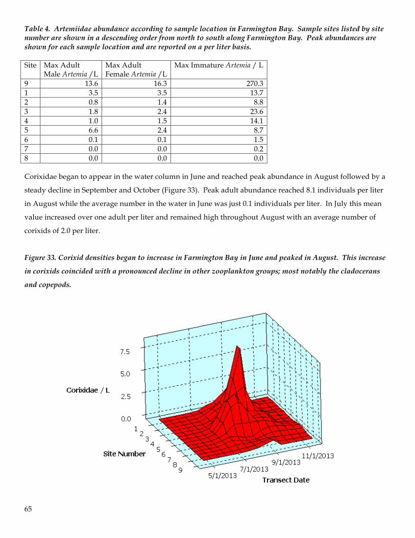
65
Table 4. Artemiidae abundance according to sample location in Farmington Bay. Sample sites listed by site number are shown in a descending order from north to south along Farmington Bay. Peak abundances are shown for each sample location and are reported on a per liter basis. Site Max Adult
Male Artemia /L Max Adult Female Artemia /L
Max Immature Artemia / L
9 13.6 16.3 270.3 1 3.5 3.5 13.7 2 0.8 1.4 8.8 3 1.8 2.4 23.6 4 1.0 1.5 14.1 5 6.6 2.4 8.7 6 0.1 0.1 1.5 7 0.0 0.0 0.2 8 0.0 0.0 0.0 Corixidae began to appear in the water column in June and reached peak abundance in August followed by a
steady decline in September and October (Figure 33). Peak adult abundance reached 8.1 individuals per liter
in August while the average number in the water in June was just 0.1 individuals per liter. In July this mean
value increased over one adult per liter and remained high throughout August with an average number of
corixids of 2.0 per liter.
Figure 33. Corixid densities began to increase in Farmington Bay in June and peaked in August. This increase
in corixids coincided with a pronounced decline in other zooplankton groups; most notably the cladocerans
and copepods.
66
The spatial and temporal heterogeneity of zooplankton in Farmington Bay illustrates the pronounced need for
frequent sampling and for a sampling program that includes multiple sites across the bay. The fact that there
is often a north-south salinity gradient, and that salinity is well established to be a driving factor in the
distribution of phytoplankton and zooplankton, is just one clear reason for the need to have multiple sample
sites that capture the status of biota within representative hydrological/hydrochemical zones of the bay.
Furthermore, identifying and assessing such trophic relationships with small-scale physical and chemical
constraints taken into consideration would enhance evaluating interactions among the biota of the bay. This
same approach applies to evaluating local abundances versus bay-wide averages; average abundances are less
useful in terms of documenting and interpreting the dynamics of phytoplankton and zooplankton in
Farmington Bay. Of greater interest are the spatially discrete counts of individuals and the dynamics of the
zooplankton at sites where peak abundance occurs.
Whereas the current study of Farmington Bay was just the first year in a multi-year effort to understand the
ecological dynamics of the bay with respect to nutrient loads and cyanobacteria blooms, the zooplankton
results provide some valuable insight into the very important role that the substantial abundance and diversity
of zooplankton play in the GSL ecosystem. The magnitude of the zooplankton biomass coupled with the
diversity serves to provide predatory avifauna with multiple prey choices in the spring and early summer, and
fewer options in mid-summer and fall. The biological basis for this shift in diversity and abundance may be
attributable to the influence of top-down effects via invertebrate predation and perhaps in combination with
other environmental factors that constrain or limit zooplankton population growth.
Spatial relationships of Farmington Bay macroinvertebrates
NMS analyses resulted in an excellent three dimensional ordination (Figure 34, final stress = 8.0%), which
explained 94 % of the variability in the distance matrix (axis 1 R2 = 0.68, axis 2 R2 = 0.15, and axis 3 R2 = 0.11).
The dissimilarities of the macroinvertebrate assemblages were well defined by site and date. Several of the
taxa contributed to define Axis 1; primarly Brachionus plicatillis, Moina macrocarpa, Leptodiaptomus connexus, and
Cletocamptus sp.(left side of Axis 1) and Trichocorixa verticalis (right side of Axis 1). Axis 2 was primarily
defined by Artemia franciscana. Because the final stress of the NMS ordination was < 10%, interpretation of
assemblage relationships is straightforward with little chance of misinterpretation (McCune and Grace 2002).
Salinity was greater moving towards the right of Axis 1 and to the top of Axis 2.
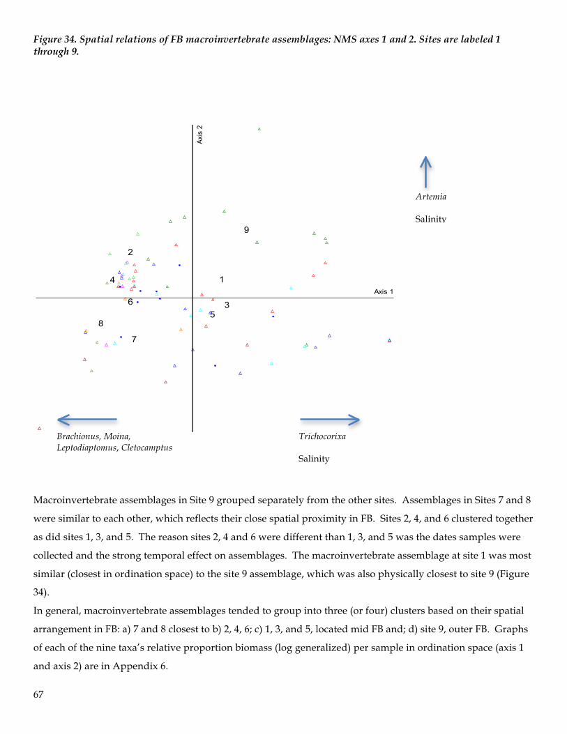
67
Figure 34. Spatial relations of FB macroinvertebrate assemblages: NMS axes 1 and 2. Sites are labeled 1 through 9.
Macroinvertebrate assemblages in Site 9 grouped separately from the other sites. Assemblages in Sites 7 and 8
were similar to each other, which reflects their close spatial proximity in FB. Sites 2, 4, and 6 clustered together
as did sites 1, 3, and 5. The reason sites 2, 4 and 6 were different than 1, 3, and 5 was the dates samples were
collected and the strong temporal effect on assemblages. The macroinvertebrate assemblage at site 1 was most
similar (closest in ordination space) to the site 9 assemblage, which was also physically closest to site 9 (Figure
34).
In general, macroinvertebrate assemblages tended to group into three (or four) clusters based on their spatial
arrangement in FB: a) 7 and 8 closest to b) 2, 4, 6; c) 1, 3, and 5, located mid FB and; d) site 9, outer FB. Graphs
of each of the nine taxa’s relative proportion biomass (log generalized) per sample in ordination space (axis 1
and axis 2) are in Appendix 6.
1
2
3
4
56
7
8
9
Axis 1
Axis
2
Brachionus, Moina, Leptodiaptomus, Cletocamptus
Artemia Salinity
Trichocorixa Salinity
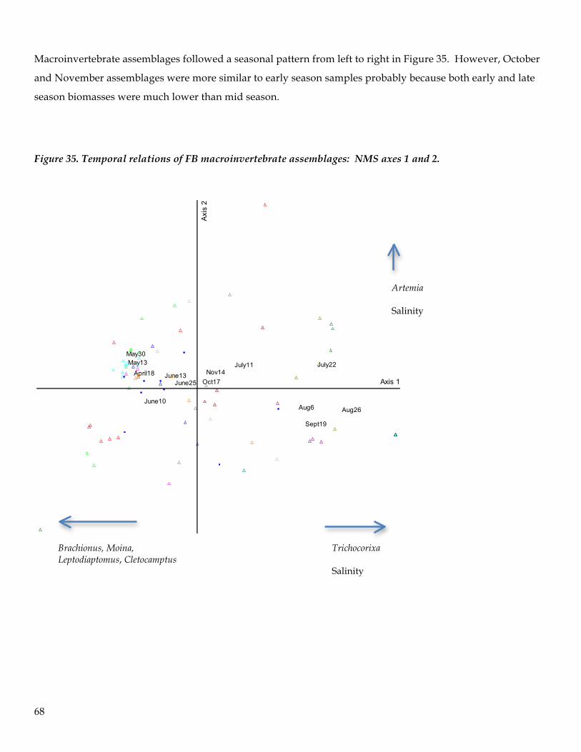
68
Macroinvertebrate assemblages followed a seasonal pattern from left to right in Figure 35. However, October
and November assemblages were more similar to early season samples probably because both early and late
season biomasses were much lower than mid season.
Figure 35. Temporal relations of FB macroinvertebrate assemblages: NMS axes 1 and 2.
April18May13May30
June10
June13June25
July11 July22
Aug6 Aug26
Sept19
Oct17Nov14
Axis 1
Axi
s 2
Brachionus, Moina, Leptodiaptomus, Cletocamptus
Trichocorixa Salinity
Artemia Salinity
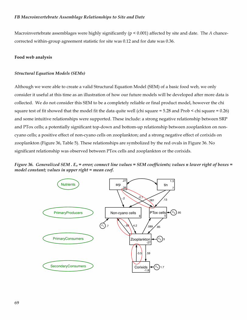
69
FB Macroinvertebrate Assemblage Relationships to Site and Date
Macroinvertebrate assemblages were highly significantly (p < 0.001) affected by site and date. The A chance-
corrected within-group agreement statistic for site was 0.12 and for date was 0.36.
Food web analysis
Structural Equation Models (SEMs)
Although we were able to create a valid Structural Equation Model (SEM) of a basic food web, we only
consider it useful at this time as an illustration of how our future models will be developed after more data is
collected. We do not consider this SEM to be a completely reliable or final product model, however the chi
square test of fit showed that the model fit the data quite well (chi square = 5.28 and Prob < chi square = 0.26)
and some intuitive relationships were supported. These include: a strong negative relationship between SRP
and PTox cells; a potentially significant top-down and bottom-up relationship between zooplankton on non-
cyano cells; a positive effect of non-cyano cells on zooplankton; and a strong negative effect of corixids on
zooplankton (Figure 36, Table 5). These relationships are symbolized by the red ovals in Figure 36. No
significant relationship was observed between PTox cells and zooplankton or the corixids.
Figure 36. Generalized SEM . Ea = error; connect line values = SEM coefficients; values n lower right of boxes = model constant; values in upper right = mean coef.
srp.26
.27tin
7
1.3
Non-cyano cells6
ε1 .7
Zooplankton-27
ε2 3
Nutrients
PrimaryProducers PTox cells5
ε3 .95
Corixids-1.8
ε4 1.7
PrimaryConsumers
SecondaryConsumers
-.2 -.081
-.59 4.2 .85
-3.5
-2.7.13
.089
.59
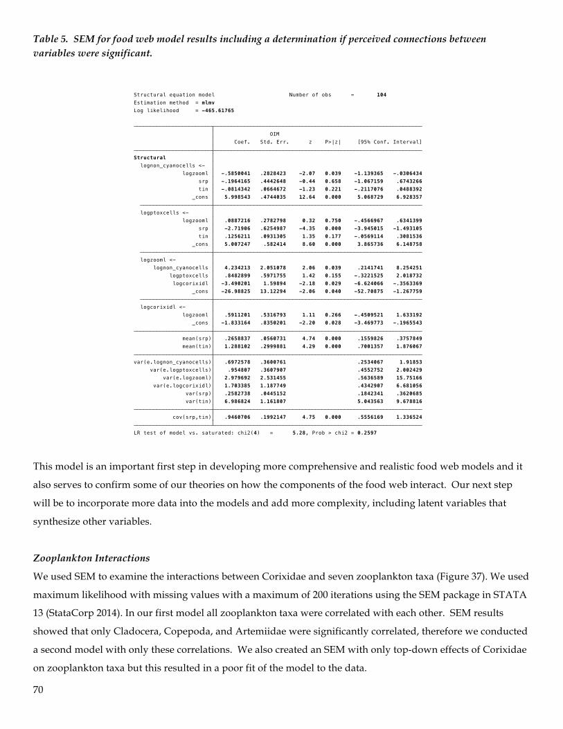
70
Table 5. SEM for food web model results including a determination if perceived connections between variables were significant.
This model is an important first step in developing more comprehensive and realistic food web models and it
also serves to confirm some of our theories on how the components of the food web interact. Our next step
will be to incorporate more data into the models and add more complexity, including latent variables that
synthesize other variables.
Zooplankton Interactions
We used SEM to examine the interactions between Corixidae and seven zooplankton taxa (Figure 37). We used
maximum likelihood with missing values with a maximum of 200 iterations using the SEM package in STATA
13 (StataCorp 2014). In our first model all zooplankton taxa were correlated with each other. SEM results
showed that only Cladocera, Copepoda, and Artemiidae were significantly correlated, therefore we conducted
a second model with only these correlations. We also created an SEM with only top-down effects of Corixidae
on zooplankton taxa but this resulted in a poor fit of the model to the data.
. LR test of model vs. saturated: chi2(4) = 5.28, Prob > chi2 = 0.2597 cov(srp,tin) .9460706 .1992147 4.75 0.000 .5556169 1.336524 var(tin) 6.986824 1.161807 5.043563 9.678816 var(srp) .2582738 .0445152 .1842341 .3620685 var(e.logcorixidl) 1.703385 1.187749 .4342907 6.681056 var(e.logzooml) 2.979692 2.531455 .5636589 15.75166 var(e.logptoxcells) .954807 .3607907 .4552752 2.002429var(e.lognon_cyanocells) .6972578 .3600761 .2534067 1.91853 mean(tin) 1.288102 .2999881 4.29 0.000 .7001357 1.876067 mean(srp) .2658837 .0560731 4.74 0.000 .1559826 .3757849 _cons -1.833164 .8350201 -2.20 0.028 -3.469773 -.1965543 logzooml .5911201 .5316793 1.11 0.266 -.4509521 1.633192 logcorixidl <- _cons -26.98825 13.12294 -2.06 0.040 -52.70875 -1.267759 logcorixidl -3.490201 1.59894 -2.18 0.029 -6.624066 -.3563369 logptoxcells .8482899 .5971755 1.42 0.155 -.3221525 2.018732 lognon_cyanocells 4.234213 2.051078 2.06 0.039 .2141741 8.254251 logzooml <- _cons 5.007247 .582414 8.60 0.000 3.865736 6.148758 tin .1256211 .0931305 1.35 0.177 -.0569114 .3081536 srp -2.71906 .6254987 -4.35 0.000 -3.945015 -1.493105 logzooml .0887216 .2782798 0.32 0.750 -.4566967 .6341399 logptoxcells <- _cons 5.998543 .4744035 12.64 0.000 5.068729 6.928357 tin -.0814342 .0664672 -1.23 0.221 -.2117076 .0488392 srp -.1964165 .4442648 -0.44 0.658 -1.067159 .6743266 logzooml -.5850041 .2828423 -2.07 0.039 -1.139365 -.0306434 lognon_cyanocells <- Structural Coef. Std. Err. z P>|z| [95% Conf. Interval] OIM
Log likelihood = -465.61765Estimation method = mlmvStructural equation model Number of obs = 104
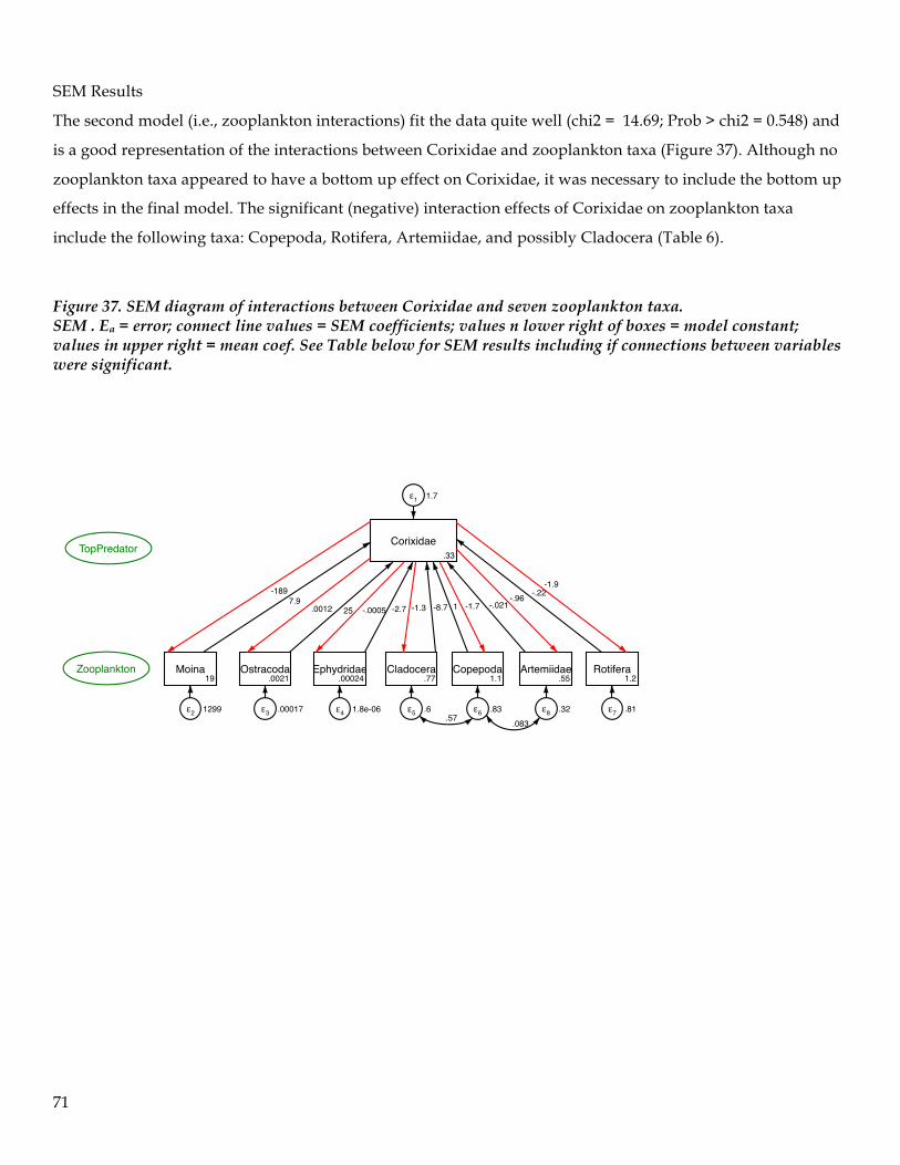
71
SEM Results
The second model (i.e., zooplankton interactions) fit the data quite well (chi2 = 14.69; Prob > chi2 = 0.548) and
is a good representation of the interactions between Corixidae and zooplankton taxa (Figure 37). Although no
zooplankton taxa appeared to have a bottom up effect on Corixidae, it was necessary to include the bottom up
effects in the final model. The significant (negative) interaction effects of Corixidae on zooplankton taxa
include the following taxa: Copepoda, Rotifera, Artemiidae, and possibly Cladocera (Table 6).
Figure 37. SEM diagram of interactions between Corixidae and seven zooplankton taxa. SEM . Ea = error; connect line values = SEM coefficients; values n lower right of boxes = model constant; values in upper right = mean coef. See Table below for SEM results including if connections between variables were significant.
Corixidae.33
ε1 1.7
Moina19
ε2 1299
Ostracoda.0021
ε3 .00017
Ephydridae.00024
ε4 1.8e-06
Cladocera.77
ε5 .6
Copepoda1.1
ε6 .83
Rotifera1.2
ε7 .81
Artemiidae.55
ε8 .32
TopPredator
Zooplankton
7.925 -2.7 -8.7 1
-.22-.021
-189
.0012 -.0005 -1.3 -1.7
.57
-1.9-.96
.083
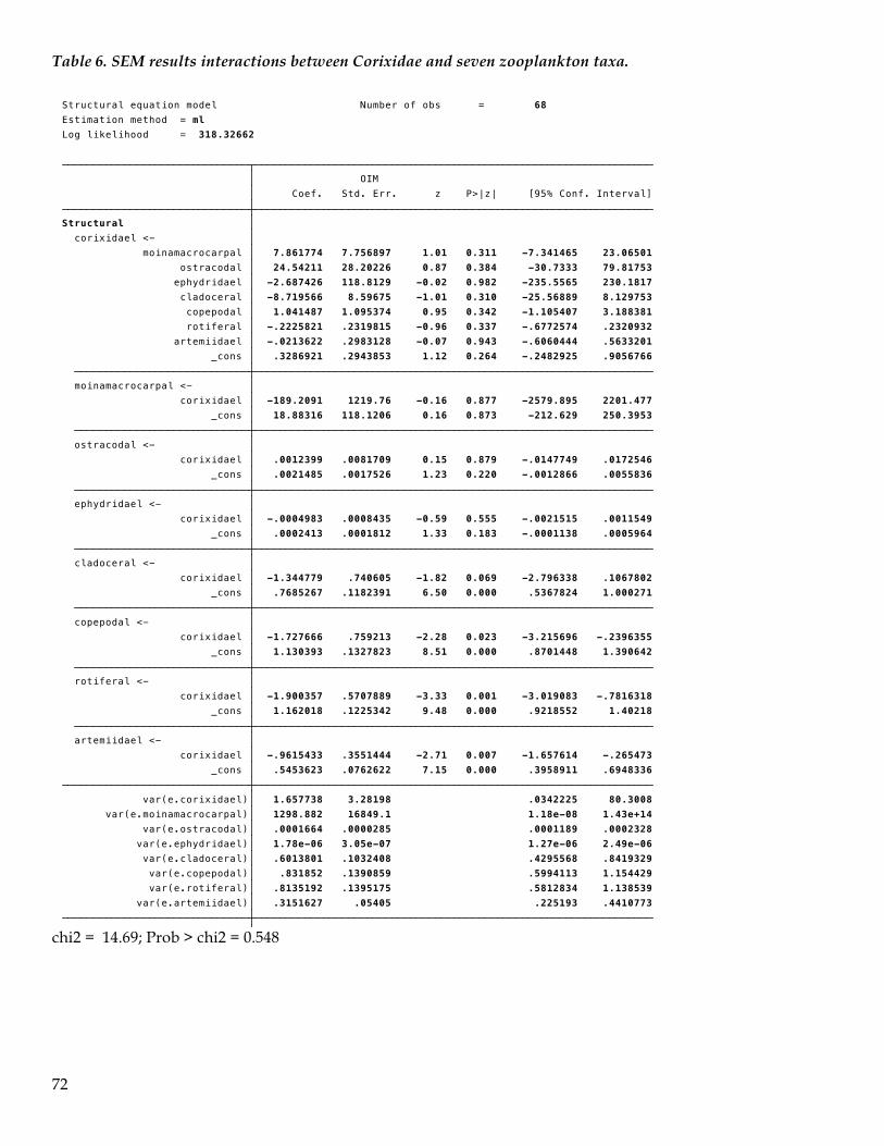
72
Table 6. SEM results interactions between Corixidae and seven zooplankton taxa.
chi2 = 14.69; Prob > chi2 = 0.548
cov(e.copepodal,e.artemiidael) .0831262 .0381387 2.18 0.029 .0083757 .1578768 cov(e.cladoceral,e.copepodal) .5731719 .1098594 5.22 0.000 .3578514 .7884925 var(e.artemiidael) .3151627 .05405 .225193 .4410773 var(e.rotiferal) .8135192 .1395175 .5812834 1.138539 var(e.copepodal) .831852 .1390859 .5994113 1.154429 var(e.cladoceral) .6013801 .1032408 .4295568 .8419329 var(e.ephydridael) 1.78e-06 3.05e-07 1.27e-06 2.49e-06 var(e.ostracodal) .0001664 .0000285 .0001189 .0002328 var(e.moinamacrocarpal) 1298.882 16849.1 1.18e-08 1.43e+14 var(e.corixidael) 1.657738 3.28198 .0342225 80.3008 _cons .5453623 .0762622 7.15 0.000 .3958911 .6948336 corixidael -.9615433 .3551444 -2.71 0.007 -1.657614 -.265473 artemiidael <- _cons 1.162018 .1225342 9.48 0.000 .9218552 1.40218 corixidael -1.900357 .5707889 -3.33 0.001 -3.019083 -.7816318 rotiferal <- _cons 1.130393 .1327823 8.51 0.000 .8701448 1.390642 corixidael -1.727666 .759213 -2.28 0.023 -3.215696 -.2396355 copepodal <- _cons .7685267 .1182391 6.50 0.000 .5367824 1.000271 corixidael -1.344779 .740605 -1.82 0.069 -2.796338 .1067802 cladoceral <- _cons .0002413 .0001812 1.33 0.183 -.0001138 .0005964 corixidael -.0004983 .0008435 -0.59 0.555 -.0021515 .0011549 ephydridael <- _cons .0021485 .0017526 1.23 0.220 -.0012866 .0055836 corixidael .0012399 .0081709 0.15 0.879 -.0147749 .0172546 ostracodal <- _cons 18.88316 118.1206 0.16 0.873 -212.629 250.3953 corixidael -189.2091 1219.76 -0.16 0.877 -2579.895 2201.477 moinamacrocarpal <- _cons .3286921 .2943853 1.12 0.264 -.2482925 .9056766 artemiidael -.0213622 .2983128 -0.07 0.943 -.6060444 .5633201 rotiferal -.2225821 .2319815 -0.96 0.337 -.6772574 .2320932 copepodal 1.041487 1.095374 0.95 0.342 -1.105407 3.188381 cladoceral -8.719566 8.59675 -1.01 0.310 -25.56889 8.129753 ephydridael -2.687426 118.8129 -0.02 0.982 -235.5565 230.1817 ostracodal 24.54211 28.20226 0.87 0.384 -30.7333 79.81753 moinamacrocarpal 7.861774 7.756897 1.01 0.311 -7.341465 23.06501 corixidael <- Structural Coef. Std. Err. z P>|z| [95% Conf. Interval] OIM
Log likelihood = 318.32662Estimation method = mlStructural equation model Number of obs = 68

73
Cyanobacteria Food Web Model
A conceptual food web model for Nodularia growth in Farmington Bay is shown in Figure 38. Although SEM
analysis was developed, such a food web model would greatly benefit from, and be more statistically robust,
with additional data. Therefore this refined model is presented at this point to illustrate the linkages to be
examined and to assist in the identification of data gaps that need to be filled with more extensive
investigations.
Figure 38. Conceptual food web model of Nodularia and the primary factors influencing its growth and expansion on Farmington Bay. This conceptual model is a useful tool for identifying data gaps and prioritizing research needs for subsequent investigations.
Nodularia
!1
Corixids
Light
Zooplankton!2
SalinityDO NutrientsTemp
Other Primary Producers !3
74
DISCUSSION Zooplankton: Predator-prey relationships, trophic interactions: top-down and bottom-up effects. Zooplankton abundance and diversity of the zooplankton assemblages were observed and recorded. There
were clear spatial and temporal changes in the zooplankton abundance. Although salt-tolerant Artemia were
recorded in the northern portion of the bay near the Antelope Island causeway, meso-haline-adapted
invertebrates dominate the remainder of the bay. Rotifers were the dominant zooplankter in June and then
again in November. Their population decline was followed by an increase in cladocerans, which yielded
dominance to copepods in some locations—primarily in the north-central region of the bay; the region that
often had the highest cyanobacteria counts. The temporal and spatial pattern observed in this study
corresponded to previous studies on zooplankton on Farmington Bay in which cladocerans (primarily Moina
sp. and Daphnia sp.) were found in substantial concentrations in May, but showed a diminished presence in
the bay thereafter (Wurtsbaugh et al., 2010). These authors also recorded depletion in zooplankton abundance
during mid-summer once the number of corixid adults started increasing and eventually reached densities of
0.5 per liter or higher. Corixid eggs are known to hatch between 20-36C (Kelts, 1979) and this may indicate
why the emergence of Corixids as a dominant zooplankter began in June when water temperature was
sustained at or above 20C. Corixid adults appeared in meaningful densities in mid-June and remained until
the end of September. Corixids have four advantages over other zooplankton: 1) they are air-breathers and are
therefore not harmed by anoxic or hypoxic events; 2) they are predators of most other zooplankton; 3) they are
omnivorous and can exploit a variety of food sources; and 4) they have piercing mouth parts that can be used
to pierce filamentous algae, that are too large for most other zooplankton to consume, and ingest the contents
(Cheng, 1976). It is not surprising then that throughout the time period of corixid abundance other
zooplankton were found in low numbers.
Other invertebrates such as the Chironomids were occasionally identified but were quite patchy in their
distribution and were found in substantially lower abundance numbers. Their presence nevertheless
represents an additional and potentially important alternative food source for shorebirds and waterbirds. For
example, Miller, Hoven and Cavitt (2009) found that corixids and midges (Chironomidae) were the main prey
items identified in the stomach contents of shorebirds such as American avocets and black-necked stilts.
Clearly the diversity of invertebrates found in Farmington Bay is a highly important element included in the
beneficial use of “support for waterfowl and shorebirds and the aquatic life in their food chain”.
The early (i.e., pre-Corixid time period) dynamics of cladocerans and copepods may be a function of their
selective or generalist grazing habits. Cladocerans, especially the large-bodied ones like Daphnia are generalist
75
feeders and may encounter foraging stress sooner in the presence of filamentous algal blooms, whereas many
of the copepods are selective grazers and have been shown to have a greater capacity to exploit alternative
phytoplankton, or protists, during times of cyanobacteria dominance (Ger, Hansson and Lurling, 2014). Other
investigators such as Fulton and Paerl, (1988) and Hansson et al. (2007) have observed shifts in zooplankton
population composition as a result of adaptations among the zooplankters. In particular, the copepods exhibit
selective feeding capabilities that allow them to forage for alternative food sources in the midst of a
cyanobacteria bloom. These authors additionally commented that cyanobacteria blooms did not favor
dominance by rotifers—an observation somewhat consistent with rotifer population dynamics in Farmington
Bay during our study in which peak rotifer abundance occurred prior to and after peak cyanobacteria blooms.
In the present study, cladocerans, such as Moina, were disproportionately abundant relative to other species,
which may be a function of their tolerance of cyanobacteria. Moina population size remained relative stable
throughout May and June--months over which Nodularia densities were at their peak. In contrast, the larger-
bodied, and generally more sensitive species, Daphnia dentifera was identified in plankton net hauls in notable
numbers (0.2 to 38.7 individuals per liter) only during April and May. They declined in number well in
advance of the presence of corixids, but consistent with the progression of cyanobacteria blooms in May,
thereby suggesting vulnerability to conditions dominated by filamentous algae. In contrast, Moina abundance
was in the range of 17 to 243 individuals per liter throughout May and June in spite of tremendous growth of
the cyanobacteria population. Numbers of Moina did not coincidentally decline with the emergence of
cyanobacteria dominance, but instead appeared to be more influenced by corixid predation. Other authors
such as Gustafsson support this relative tolerance of cyanobacteria by Moina compared to Daphnia and
Hansson (2004) and Guo and Xie (2006) who found that the smaller cladocerans like Moina and Ceriodaphnia
develop tolerance to cyanobacteria better than the larger bodied Daphnia.
Depletion of algal species, such as diatoms, coinciding with increases in known phytoplanktivorous species
suggests important predator-prey or grazing relationships that shape the temporal and spatial abundance and
population structure of phytoplankton. Evidence of grazing pressure caused by the zooplankters was
indicated by the phytoplankton population fluctuations and responses. Zooplankton grazers such as the
cladocerans and Artemia have the capacity to graze near 100% of the water column per day according to
studies conducted by Wurtsbaugh (2012). In the current study the results were consistent with “top-down”
control of algal dominance in the presence of substantial grazing pressure: when algal grazers such as the
cladocerans and Artemia were present the densities of “edible” algae were held in check. However, once the
grazing pressure of these zooplankters diminished, for example during July, the densities of “edible”
phytoplankton, such as the chlorophytes, showed signs of resurgence in abundance.
76
Predation of other zooplankton by corixids was anticipated based on observations of previous investigations
(Wurtsbaugh, 1992; Tanner, Glen and Moore, 1999; Cheng, 1976; Reynolds, 1975) and from our own laboratory
studies demonstrating predator-prey relationships between corixids and Artemia. Of particular importance are
the observations of Simonis (2013a) that all instars of Trichocorixa verticalis preferentially prey on Moina in food
preference studies and that prey by corixids creates a top-down cascade releasing phytoplankton from grazing
pressure. Additionally Wurtsbaugh and Berry (1989) reported that Trichocorixa verticalis invaded the pelagic
region of the GSL when the salinity dropped from around 100 g/L to 50 g/L and as a result initiated a
cascading trophic shift in the food web structure by depleting the phytoplanktivore Artemia. In an
investigation of rock-pool communities Simonis (2013b) found that Moina population density is the primary
factor influencing emigration of Trichocorixa verticalis—at certain low abundances of Moina the corixids will
leave their current ponds and exploit other ponds with greater abundance of Moina. They further found that
T. verticalis are “voracious predators” of Moina macrocapa. In our study there was definitive progression of
depletion of cladocerans, copepods, rotifers, and Artemia when corixids were in an adult abundance of more
than 1 mature adult/L. This progression of population decline was observed both temporally, beginning in
June, and spatially, with corixids reaching maturity first in the southern region of the bay and then over time
moving in a south-northward expansion of dominance in zooplankton assemblage. Although the evidence
indicates pronounced top-down control by corixids, the decline in the abundance and diversity of zooplankton
may not be solely attributed to corixid predation as it may be a combined function of predation coupled with
intra- and interspecific competition, normal life-cycle sequences of development, growth and mortality, food
limitation, temperature tolerances, dissolved oxygen levels or the presence of cyanotoxins. Yet the
combination of controlled laboratory experiments that documented corixid predation rates, coupled with the
correlation between corixid presence and the decline of other zooplankton, followed by recovery of other
zooplankton once corixid numbers were in decline, all strongly support top-down control mechanism of
zooplankton abundance in Farmington Bay by corixids. This top-down control appears to be a more
significant factor regulating zooplankton population size and diversity than direct adverse impacts of
cyanobacteria blooms on the zooplankton.
The trophic transfer of energy, nutrients, carbon and other essential elements and compounds is most certainly
influenced by phytoplanktivory rates among the various zooplankton species. It is well established in the
scientific literature that the type of algae available exerts an influence on grazing rates and digestibility of
consumed food by zooplankton (Gibor, 1956). While there are substantial differences in grazing rates and
digestibility among the various divisions of algae—for example cyanobacteria (division Cyanophyta)
compared to diatoms (division Chrysophyta) and green algae (division Chlorophyta)—there are even
differences within the families or genera of phytoplankton (Tanner et al., 1999). For example, Gibor (1956)
found that differences existed even within the same genera of green algae: he observed that Dunaliella viridis
77
was superior over D. salina when grazed by Artemia. He also found that Artemia could selectively graze one type
of green algae in preference to other less desirable and less digestible species. In his study the Artemia grazed
selectively on D. viridis over Stichococcus. Gibor also reported that Stichococcus cells that passed through the
digestive system of the Artemia remained viable. In similar studies Tanner et.al. (1999) observed that
equivalent populations of Artemia in salt ponds had very different impacts on the abundance of algae; they
found that Artemia grazed diatoms down to low densities (only 1,250 cells per mL), whereas when the
cyanobacteria Synechococcus was present more than 4.2 million cells per mL remained in spite of the same
density of adult Artemia. They also found that when Artemia were not present the salt ponds contained high
numbers of diatoms, thereby supporting the hypothesis that selective algal grazing by Artemia can determine
the algal species composition of salt ponds. These and other studies illustrate the importance of food quality
on zooplankton and the pressure that they exert on competition, growth and survival among the invertebrate
grazers. In Farmington Bay this has particular relevance because phytoplankton of presumed high quality,
such as diatoms and green algae, are displaced by filamentous cyanobacteria resulting in suboptimal forage
for a diversity of zooplankters.
Artemia were found primarily in the central to northern regions of Farmington Bay and their distribution was
influenced by salinity. It is well known that Artemia are classic extremeophiles (Hengherr, Schill and Clegg,
2007) that exhibit a remarkable capacity to withstand hypoxia and a vast range of salinities, ranging from
marine water to saturated brines. It is in this capacity that they derive a competitive advantage over other
zooplankters. They are known to demonstrate selective feeding capacities and can survive given a wide range
of phytoplankton options as long as the size of algal cells is sufficiently small (i.e., 4-8 microns for metanauplii
and <20 microns for adults) to pass their feeding apparatus (Makridis, P., & Vadstein, O., 1999). In our study
there were periodic periods of high abundance in the northern regions of the bay (20.6/L to 27.9/L) while peak
abundance in sites 6, 7& 8 (southernmost sites in our study) the Artemia only achieved a maximal value of 1.73,
0.18, and 0.00/L respectively. The low salinity of this region of Farmington Bay did not support Artemia
growth and development likely due to interspecific competition and predation pressure. In contrast, at site #9,
just on the north side of the Antelope Island causeway breach, the peak value for total number of Artemia
reached 300.1/L. Within the northern section of Farmington Bay (defined as sites 1, 2, & 3) the mean salinity
ranged from 2.4% to 4.1% and the highest observed at site #1 was 8.2%. These are well below values for site #9
where the average salinity was 11.1% and the high was 14.0%. Clearly the salinity of site #9 conferred some
advantage for Artemia over other zooplankton as well as relieving the Artemia from the predation pressure of
corixids—the average number of corixids per liter at this site was a mere 0.09/L and the maximum value was
0.69/L. In previous work on Farmington Bay by Wurtsbaugh and Marcarelli (2004) they found that corixid
abundance of just 0.28/L was sufficient to control Artemia population size, whereas the lower corixid
abundance they observed in 2003 (0.06/L) did not control the Artemia population size.
78
Artemia abundance in sites 1- 5 were comparable to reports in the literature of Artemia abundance in
Farmington and Gilbert Bay. In our study Artemia mean values for these sites were between 1.84 and 6.64
individuals/L with a peak abundance range of 8.81 to 27.91/L. These peak values are more than were
reported by Stephens and Gillespie (1976) for Gilbert Bay in which they found that 12-15 individuals per liter
was the upper limit for Artemia. Wurtsbaugh and Gliwicz (2001) present a mean value for adult Artemia in
Gilbert Bay of 3.1/L and compare this to a more productive Mono Lake that boasts 6-8/L. These values, and
the average abundance we observed for site #9 in our study (4.62/L) are well above the mean values for
Artemia abundance even in the northern zone of Farmington Bay (0.75/L to 0.85/L). Collectively this indicates
that a variety of conditions in Farmington Bay such as competition, predation, and food availability maintain
the Artemia population below more productive levels observed when salinity is higher and Artemia have an
ecological advantage, such as in Gilbert Bay.
Phytoplankton and Chlorophyll-a There was a remarkable diversity of algal taxa observed in the current study: 10 major taxa, 81 genera and
more than 50 species of algae were collected and identified. This is greater diversity than some of the
previously reported values for Farmington Bay (Wurtsbaugh, Marcarelli, and Boyer, 2012) and may be a result
of the thoroughness and frequency of the sampling program and area of the bay that was sampled. It is also
greater diversity than was found in the other more saline bays of the GSL. The decrease in diversity of species
observed in the other bays of the GSL is an expected outcome of the diminishing effect that increases in salinity
has on algal and zooplankton species diversity (but not necessarily on the bacterial populations). One of the
factors that favored species richness during the course of our study was the low level of the GSL (elevation
between 4194 and 4197 and approaching the lowest level ever recorded—4191 feet above sea level). This low
elevation of Gilbert Bay results in most of Farmington Bay being in the lower range of salinity (i.e., 0%-6%).
Previous studies of Farmington Bay that reported less diversity also recorded higher salinity across the bay—
with salinities ranging from 4% to 10% (Wurtsbaugh and Marcarelli, 2006), 1% to 9% (Wurtsbaugh, Marcarelli,
and Boyer, 2012). The low elevation and therefore low salinity of Farmington Bay during 2013 favored the
growth of cyanobacteria.
Farmington Bay is a highly dynamic water body characterized by constant production, movement, mixing,
grazing, and ultimately decline of algal species. In the midst of this perpetual change there are patterns that
emerge and that can be identified and characterized. Clearly the most apparent pattern is the emergence and
dominance of the cyanobacteria bloom that begins in May and results in pronounced dominance of the algal
assemblage that continues well into September. This is consistent with a variety of earlier studies that are
reviewed in great detail in Wurtsbaugh, Marcarelli, and Boyer (2012). In this publication they cite multiple
79
earlier investigations of Farmington Bay that also recorded cyanobacteria blooms starting in May and
extending into the fall. One difference in our study from some of the previously reports is that while Nodularia
was the early and dominant cyanobacteria it was displaced in dominance by Pseudanabaena in August. In most
of the studies reported by Wurtsbaugh this dramatic increase in Pseudanabaena is not reported, yet Aphanothece
does show up in some of the studies at high abundances. In a thorough investigation of Farmington Bay by
Wurtsbaugh in 2009 (cited in Wurtsbaugh et al., 2012) Nodularia represented 91% of the total cyanobacteria and
86% of the total algae in Farmington Bay. In this same publication Wurtsbaugh et al., had similar results to our
study in which the southern locations in the bay, with salinities in the range of 1% to 3%, did not support
cyanobacteria blooms. Their interpretation of the cause is consistent with ours: exclusion of cyanobacteria
from this region of the bay is due to available nitrogen from input sources (mainly discharges by POTWs) that
create an environment which favors other algal groups and not nitrogen fixing filamentous algae. Another
consistent finding is that there is a salinity threshold for Nodularia: both in our study and in a summary of
findings from 2002, 2003, 2005 and 2009: the upper threshold limit for Nodularia at approximately 6% salinity
(Wurtsbaugh et al., 2012). Roney (2009) also reported on the exclusion of specific cyanobacteria species as a
result of salinity.
As a point of clarification, the generally accepted definition of the term “algal bloom” indicates the emergence
of a particular algal group that represents >50% of the total algal population. Throughout this report the term
“bloom” is used to reference the rapid appearance of a particular algal group, and of a magnitude approaching
or exceeding 50% of all represented algae. Among the algal groups that were documented during this study
only the cyanobacteria and diatoms demonstrated “large algal blooms” that resulted in dominance of a
particular group of more than 50%. Hence these two taxa are the predominant algal groups in Farmington Bay
during the course of our study. Chlorophytes never achieved this degree of dominance, but they did show a
pattern of pronounced resurgence once grazing pressure was diminished in July through September.
In the early spring the bay supports the growth and development of edible and desirable algal groups for
zooplankton grazers. Among these are the diatoms and chlorophytes. Other algal groups such as the
cryptophytes, chrysophytes, pyrrhophytes, and flagellates that periodically make notable appearances in the
bay, albeit at far lower abundance, than the three main algal groups: cyanophytes, bacillariophytes, and
chlorophytes. Close scrutiny of the dynamics of each of the algal groups provides some insight into the
relationship between nutrients, algae and zooplankton grazers and the patterns of abundance. There is
evidence that grazing pressure coupled with nutrient availability, salinity, and temperature all interact to
select patterns of algal dominance. Tanner et al. (1999) found Artemia to selectively graze chlorophytes and
diatoms in preference to cyanobacteria. The conditions that favor cyanobacteria are readily available
phosphorous, nitrogen limitation, salinity below 6%, water temperature over 20C, and a reduction in grazing
80
pressure by zooplankton. In a separate experiment, Wurtsbaugh and Marcarelli (2004) did controlled studies
of nitrogen-fixing bacteria growth under differing conditions of nutrients and salinity. They found that
growth of nitrogen-fixing algae occurs below 7% salinity. Our field research does not provide a definitive
range of factors that favor the presence of diatoms or green algae over the nitrogen fixing algae, but some
general observations are that nitrogen availability (and in particular the bioavailable forms of nitrate or nitrite
and ammonia), salinity of 6%or greater, and reductions in grazing pressure, lend some support to the growth
of these algal divisions. Additionally, reductions in the shading effects caused by the extensive cyanobacteria
blooms—an event which happens when the blue-green algae “scums” settle to the bottom of the bay—also
confer some advantage to other algal groups.
The sheer magnitude and persistence of the Nodularia bloom that occurred in late May and extended into late
fall, and the subsequent Pseudanabaena bloom in August-September, are indicative of a trophic barrier to the
transfer of nutrients and carbon through the food web (Ger, Hansson and Lurling, 2014). In this capacity it
represents a significant “bottleneck” to the potential capability of Farmington Bay to transfer nutrients and
energy up trophic levels and to support the growth and development of higher level grazers and predators. It
is therefore a stark limiting factor to the potential secondary and tertiary productivity of the bay.
Farmington Bay is quite different from Gilbert Bay and the wetlands that border the eastern, northern and
southern margins of the GSL. In this study of the phytoplankton flora of GSL wetlands Rushforth and
Rushforth (2004) found the order of importance was pinnate diatoms>centric
diatoms>chlorophytes>cyanophytes. In their study of ten different wetlands these authors attributed 83% of
the summed index of importance to diatoms. It is noteworthy when making comparisons among regions of
the bay to include temporal effects; in the Rushforth study the wetlands were only sampled in October and
November—months in which the cyanobacteria were already in their decline in Farmington Bay. In our study
clearly the dominance pattern differed from the surrounding wetlands and was
cyanophytes>diatoms>chlorophytes.
Algal assemblages differ in very profound ways in Farmington Bay compared to the other bays of the GSL.
For example, during 1972 and 1973 Stephens and Gillespie found that the algal flora of Gilbert Bay was
essentially limited to just two species: Dunaliella viridis and an unidentified green algae. In a 1998 paper
Stephens reports only 6 species of algae in Gunnison Bay and 15 species of algae in Gilbert Bay. This low level
of diversity in Gilbert Bay during times of high salinity reveals one of the very important aspects of
Farmington Bay—its diversity and the role that said diversity of algae and zooplankton serve in terms of
beneficial uses. A broad variety of conditions that supports an array of zooplankton in turn provides much
81
greater diversity of prey choices for the tens-of-thousands of waterbirds and shorebirds that utilize
Farmington Bay and its surrounding environs.
Chlorophyll-a levels reached exceedingly high values at various times and locations during this study. The
mean chlorophyll for the entire study was114.6 ug/L and the highest value recorded was 506.0 ug/L. This is
quite similar to previous studies in which the mean chlorophyll level from 2002 to 2009 was 141 ug/L
(Wurtsbaugh et al., 2012). Throughout our study the chlorophyll levels were above the generally accepted
value for hypereutrophic conditions of 56 ug/L (Carlson and Simpson, 1996). An exception to this occurred at
sites 7 and 8 where peak values were 45.4 and 32.7 ug/L respectively. The mean values at these locations
were: 29.8 and 32.4 ug/L. These are well below the mean values for sites 1-6 that had mean values of 131 to
291 ug/L and maximum values that were between 373.8 and 506.0 ug/L. These are extremely high values for
chlorophyll and are associated with robust primary production and in particular cyanobacteria blooms.
Cyanotoxins
Cyanotoxins are a huge concern in association with cyanobacteria blooms. The presence of cyanotoxins is well
known to accompany blue-green algae blooms; for example, Antoniou, de la Cruz and Dionysiou (2005) state
that up to 50% of all recorded cyanobacteria blooms contain cyanotoxins. Cyanotoxins are known to harm
resident biota, contaminate ground water, and can be toxic to humans via dermal or ingestion exposure
(Funari and Testai, 2008). The two main modes of toxicity of cyanotoxins are either via neurological or hepatic
disruption. In our study, the hepatotoxin nodularin was observed in substantial concentrations when
Nodularia abundance exceeded 10,000 cells per ml. We also analyzed for the neurotoxin Anatoxin-a, but did
not record elevated levels. Nodularin, on the other hand, was first observed in May and later reached a
maximum value of 88.0 ug/L in early June. Over the entire study the mean concentration was 13.4 ug/L and
according to the distribution of blue-green algae across the bay nodularin was highest in the mid to northern
regions of the bay and quite low among the southern sites. Nodularin continued to be found in water samples
until November. Concentrations recorded during 2013 were lower than some of the previous reported values.
In 2009 Wurtsbaugh et al. documented a bay-wide average of 41 ug/L and they report an astonishing, and
questionable, value of 600 ug/L at one site. Over a 3 year period (including 2006, 2007 and 2009), and for the
time period May to August, they reported mean values of 20, 24, and 104 ug/L respectively. In contrast to our
threshold model for nodularin these authors documented a linear relationship between microcystins and
Nodularia. It should be noted that an investigation by Goel (2007) did not arrive at the same conclusions
regarding cyanotoxins in Farmington Bay as were reported by Wurtsbaugh et al. While direct impacts of
nodularin on the biota of Farmington Bay was not evident from our field study, controlled laboratory studies
of nodularin impacts on the zooplankton that utilize Farmington Bay should be undertaken.
82
The presence of cyanotoxins in the water of Farmington Bay raises some concerns with regard to direct harm
to the biota as a result of exposure to the toxins. Various studies have demonstrated adverse impacts on
zooplankton such as Artemia as a result of cyanotoxin exposure (Lee, Chen, and Chen 1999; Kiviranta et al.,
1991). In the study by Kiviranta eta al., (1999), exposure of Artemia to 29 toxic bloom samples, they found that
only 4 out of the 29 were nontoxic to Artemia. In an investigation of detoxication mechanisms of Artemia
Beattie et al. (2003) found that Artemia have phase II conjugation enzyme systems (i.e., glutathione S-
transferase) that afford the Artemia some limited capacity to withstand nodularin exposure. Although
Anatoxin-a was not found in substantial concentrations in our study, it is a neurotoxin of potential concern. It
is produced by Anabaena flos-aquae strain NRC 525-17 and has a LD50 of a mere 20-50 ug/kg body weight in
mice; and at this level of toxicity is included in the class of potent toxins (Patocka, Gupta and Kuca, 2011). It
exerts its toxic potential via the inhibition of cholinesterase which includes it alongside some of the well
known neurotoxins, such as Sarin gas, used in chemical warfare. However, Anatoxin-a apparently does not
cross the blood-brain barrier and is unable to disrupt central nervous system neurons. It causes its harm to the
individual through impairment in peripheral nervous system tissues and neuromuscular junctions. Because of
its extreme toxicity it is prudent to continue to monitor Farmington Bay for elevated levels of Anatoxin-a. As
described above, we could not find any significant relationship between Nodularia densities and changes in
the zooplankton community. However, this is the first study that provides sufficient frequency and ecological
detail that can address the potential for this linkage. Additional monitoring and research should be conducted
to elucidate the potential for toxicity due to cyanobacteria blooms in Farmington Bay.
Dissolved oxygen and Salinity
Depletion of oxygen is one of the concerns often expressed with regard to eutrophication of water bodies. In
our study all mean daily values for the bay were above 2 mg/L. There were isolated cases of hypoxia or
anoxia in which the oxygen levels dropped below 1 mg/L. Because all of our measurements of dissolved
oxygen took place during the day the perception of impairment is lessened and anoxic events could have taken
place during the night but were unrecorded. When comparing zooplankton abundance with oxygen levels
during the day there is no clear evidence of harm to the biota. Yet, declines in oxygen during the night
remains a concern though, especially when one considers the observations of Wurtsbaugh et al. (2012) who
found that oxygen levels in the daytime could reach as high as 40 mg/L but would decline to 0 ug/L at night.
In our study oxygen levels peaked at 17.3 mg/L while the lowest values were between 0.09 to 0.39 mg/L. The
lowest levels coincided with the development and collapse of cyanobacteria blooms in May through July.
83
Observations of the abiotic factors of Farmington Bay included a well defined spatial salinity gradient
extending from the northern end of the bay near the Antelope Island causeway to the southern regions of the
bay near the various hunting club preserves and the recently exposed former lake bed. Salinity in the northern
region of the bay near sites 1-3 was typically in the range of 1% to 6%. Sites 4, 5, and 6 exhibited some influence
of salt influx from Gilbert Bay and showed salinity in the range of 0.5% to 3%. Sites 6, 7 and 8 were essentially
fresh water sites. These salinity levels are consistent with previous investigations that also documented
consistent north-south gradient across the bay (Wurtsbaugh and Marcarelli 2004; Wurtsbaugh et al., 2012).
Salinity has a strong influence on the diversity of biota found in a given water body and as salinity increases
diversity decreases. Williams (1998) found that although salinity is an important factor in the structure of
biological communities it is less influential as a determinant of community structure that is often thought, yet
Williams does support the observation that increasing salinity coincides with a decrease in species richness.
Salinity becomes a major influence at high levels but at lower levels the various salinity tolerances of
zooplankton and phytoplankton and the predator/prey relationships that emerge serve a similarly important
role in determining the overall biotic structure. In Farmington Bay perhaps the most relevant expression of
salinity tolerance is that held by cyanobacteria; and it appears that it has an upper limit of 6% to 7%. In the
combined salinity and nutrient enrichment experiments conducted by Marcarelli, Wurtsbaugh, and Griset
(2006) these investigators found that when the salinity was 70g/L nitrogen fixation ceased. Under such
conditions nitrogen can become limited rather than phosphorous. In their policy forum paper Conley et al.,
(2009) commented that significant planktonic nitrogen fixation is not observed at salinities in excess of 8% even
in circumstances of severe nitrogen limitation. These experiments illustrate that when considering nutrient
effects on a waterbody salinity must also be taken into account as a controlling factor.
This awareness of the upper threshold of cyanobacteria can potentially be used as an effective tool to restrain
the magnitude of cyanobacteria blooms in Farmington Bay rather than focusing on reductions in nutrient
input as the sole remedy for reducing harmful algal blooms. In fact, engineering solutions that enhance the
exchange of water between Gilbert Bay and Farmington Bay may be a more ecologically prudent approach to
reducing cyanobacteria blooms in the bay. It would serve a dual function of reducing cyanobacteria blooms
but also increasing the movement of nutrients into Gilbert Bay, thereby providing for enhanced growth in the
resident algal population and as a beneficial consequence it could support a larger and more productive
Artemia population. Wurtsbaugh et al. (2012) expressed concern about the impact that the Antelope Island
causeway has had on Farmington Bay and they supported the idea that greater exchange between Farmington
Bay and Gilbert Bay would have multiple beneficial outcomes. They state that the causeway has increased
residence time in the bay thereby capturing and containing the high nutrient loads and preventing them from
entering Gilbert Bay. The reduced exchange between bays has clearly lowered the salinity in Farmington Bay
into a range that favors cyanobacteria blooms. The additional benefit of improving the exchange between the
84
bays would be increased primary productivity in Gilbert Bay and as a result would be greater production of
foraging items for birds, hence an improvement in the beneficial uses of the lake. It is worth noting that
Herbst (2006) found that evaporation ponds of intermediate salinity (112 g/L) produced the best combination
of zooplankton diversity and nutritional quality in terms of foraging opportunities for shorebirds. He
observed greater usage of these ponds by birds and found that the lower salinity (98 g/L) and higher salinity
ponds (173 g/L) were suboptimal in terms of food quality and quantity for birds. The undesirable excessive
predation by corixids on zooplankton could also be mitigated by increases in salinity (Van De Neutter, Trekels,
Green and Stoks, 2010). It is worth noting however, that Miller, Hoven and Cavitt (2009) found corixids to be a
dominant prey item in shorebirds feeding in Farmington Bay and other GSL wetlands. This generally points
out the opportunistic nature of shorebird feeding behavior. Nevertheless, general increases in salinity will be
favorable in that such feeding is restricted to the shoreline of the bay, allowing greater zooplankton abundance
and diversity in deeper pelagic portions of the bay. Similarly, greater salinity would generally be restricted to
open water regions because of the innumerable tributary flows (emitting from impoundments, drains, POTW
discharges and streams) and natural springs, maintaining substantial brackish to freshwater zones that would
remain optimal to corixid and midge production. This concept of addressing the problem of cyanobacteria
blooms in Farmington Bay via increased salinity has been given some thought in earlier studies but warrants
more serious consideration as a prudent approach to solve the ecological concerns in Farmington Bay.
Nutrients: sources, gradients, and evidence of limitation.
The nutrients that were thoroughly documented during the study included various molecular forms of
nitrogen (N) and phosphorous (P). Other nutrients or essential elements were not evaluated. The results show
evidence of site-specific loading of nutrients into Farmington Bay. The primary source location is the
Northwest Oil Drain that transports the Salt Lake City POTW effluent to a discharge point located near sample
site #7. Both phosphorous and nitrogen were elevated in this area well above most other sites. All
assessments of nutrients varied temporally and spatially across the bay. TN:TP ratios were low (overall mean
value was 9.25) and were consistent with ratios expected from eutrophic systems and are indicative of N
limitation rather than P limitation. The ratio was, however, higher than the values provided in the
Wurtsbaugh et al. (2012) paper in which they found that all bays of the GSL had TN:TP ratios of 25 or higher—
indicating that in all bays of the GSL nitrogen would be adequate while phosphorous would in fact be the
limiting nutrient. This observation is counter to almost all systematic studies of nutrient limitation in the GSL,
including Wurtsbaugh’s own studies, in which nitrogen is shown to be the rate limiting nutrient and P is in
abundance.
85
The TN:TP ratio in our study finally increased over 16:1 in November (20.73) when algae growth had slowed
substantially due to low angle incidence of the sun and colder temperatures. There was also a notable increase
in the ratio of TN:TP in early June that continued to be maintained until fall. This increase likely resulted from
nitrogen fixing capacities of cyanobacteria blooms that began in May but that reached their peak in June and
July. The TN:TP ratio generally followed a south to north gradient with the lowest ratio usually found along
the southern margin of the bay and increasing ratios as the samples were progressively collected from a
northerly direction. An explanation for this observation is multi-faceted but essentially involves substantial
inputs of nitrogen and phosphorous from the Northwest Oil Drain outlet near sites 7 & 8 followed by rapid
uptake of bioavailable forms of N (nitrate, nitrite, and ammonia) and P (SRP) by algae and “downstream” of
this nitrogen uptake and depletion cyanobacteria gain a competitive advantage and grow in earnest—
increasing the TN:TP ratio and contributing nitrogen to the system.
The bioavailable forms of P and N were readily assimilated at points close to the source canal. The lack of
cyanobacteria growth relative to other forms of algae in close proximity to site #7 supports the hypothesis that
nitrogen availability diminishes the competitive advantage of cyanobacteria over other nitrogen dependent
species. The TN:TP ratio then increases in a consistent manner with the production and distribution of
cyanobacteria in the bay; grouping sites by region (7-8; 6-4; and 3-1) gives the following average ratios: 4.4;
8.12; and 10.0 respectively. The explanation for the spatial pattern (cyanobacteria production reflects nitrogen
fixation and the generation of nitrogen for biological growth) is supported by the temporal pattern in which
there are increases in TN over time and consistent with cyanobacteria growth.
The mean concentration of bioavailable forms of N and P near site #7 were higher than other sites by almost an
order of magnitude: SRP at sites #7 and #8 had an average of 0.98 to 1.29 to mg/L and a maximum value of
1.64 to 2.61 mg/L. In contrast the other sites had mean values between 0.02 to 0.14 mg/L and maximum
values of 0.04 to 1.14 mg/L. Similarly ammonia near site #7 had a mean value of 3.95 while all other sites were
between 0.22 to 0.54 mg/L. Nitrate and nitrite also showed the same type of pattern: the mean value at site #7
was 3.77 compared to a range of 0.03 to 0.28 mg/L. Consistently this was the case near site #7. Based on these
results it is quite evident that this source is one the major contributors to nutrient input into Farmington Bay.
It should also be pointed out that two additional POTWs discharge to Farmington Bay, the Central Davis and
North Davis Sewer Districts’ discharges. However, under such low lake elevations (as during the last several
years), the Central Davis discharge evaporates before it reaches the open water of the bay. The North Davis
discharge occurs approximately 500 meters from the Antelope Island causeway. While it is a substantial flow
(approximately 30 cfs), our sampling, even at site 1, did not identify any chemical, nutrient or biological
differences that could be associated with this discharge. It likely flows parallel to the causeway until it reaches
the breach where it is immediately discharged to Gilbert Bay.
86
There is a wealth of information in the scientific literature evaluating the roles of N and P in eutrophication of
water bodies. Classic long term, lake-scale, studies done by Schindler et al., (2008) found that P was the
dominant nutrient controlling eutrophication in lakes. This, and other studies, ushered in the “Phosphorous
Paradigm” in which it was recognized that implementation of P controls could effectively reduce deleterious
impacts of eutrophication on fresh water lakes and streams. Success stories, such as was encountered in Lake
Washington, following P controls bolstered the awareness of the value of P controls for improving water
quality of lakes and streams. However, there has also been much debate about the applicability of this
approach to other water bodies, especially marine or estuary systems (Smith and Schindler, 2009; Genkai-Kato
and Carpenter, 2005; Lewis and Wurtsbaugh, 2008; Sondergaard, Jensen and Jeppesen, 2003; Sondergaard,
Jensen and Jeppesen, 2001; Schindler et al., 2008; Sterner, 2008; Lewis, Wurtsbaugh and Paerl, 2011). A
synthesis of the minutiae of all of these investigations is beyond the scope of this paper, but a distillation of
ideas and observations suggests that in Farmington Bay initial reductions in P coupled with unchanged N
inputs may reduce the dominance advantage of cyanobacteria over other algal species. However, one should
recognize that changes in either N or P or the combination of them causes a shift in the pattern or status of
limitation and may also introduce unintended consequences. Furthermore, it is known from a variety of
studies (Sondergaard, Jensen and Jeppesen, 2003) that years of nutrient loading into lakes, internal cycling of
nutrients, and other biogeochemical processes can continue to supply biota with nutrients for years even with
dramatic reductions in loading of nutrients. The processes of remineralization, nitrogen fixation or
denitrification all contribute to either depletion or liberation of nutrients for assimilation into biological
systems.
Field observations can only provide a glimpse into the relative limitation, or co-limitation, of nutrients in the
bay. It is absolutely necessary to conduct laboratory and mesocosm studies of algal responses to enrichment in
order to understand the spectrum of likely outcomes of either P or N or N&P limitation on the ecological
processes in Farmington Bay. Other essential considerations of proposed reductions in nutrient input into
Farmington Bay must take into account the possible implications on other bays of the GSL and their resident
biota. Nutrient dynamics and goals of ecological conditions in the bay need to accurately understand the
broader implications of changes in nutrient input and connectivity between bays. It is possible that dramatic
reductions in nutrient input into Farmington Bay could result in diminished primary and secondary
productivity of Gilbert and Gunnison Bays. An unintended consequence of this could be reduced food
available for of avian predators that rely upon sizeable zooplankton populations. Such a change would violate
the primary beneficial use of bays of the GSL.
Eutrophication of Farmington Bay is undeniably of concern, but changes in nutrient input into the bay must
take into account a wide array of potential consequences and need to be based on rigorous science that couples

87
field observations with carefully designed and executed laboratory studies that can simulate the variety of
possible outcomes from changing nutrient input into the bay. Management of the bay needs to be an iterative,
systematic process that judiciously takes into account both short and long term goals and outcomes and that
understands the interconnectivity of Farmington Bay with the rest of the GSL.
88
SOME INITIAL RECOMMENDATIONS FOR FURTHER RESEARCH ON FARMINGTON BAY
Nutrient Enrichment Studies • Conduct both laboratory and mesocosm experiments. Laboratory studies have the advantage of being
able to control many of the variables. • Mesocosms have perhaps more practical applied relevancy, but they are prone to disruption by the
vicissitudes of the weather or demonic interventions. • Conduct experiments on both Farmington Bay and Gilbert Bay water sources collected at various times
of the year. • Add N, P, N&P • Combine salinity modifications and nutrient enrichment tests
Toxicity Testing of Cyanotoxins on Relevant Zooplankton from Farmington Bay
• Test the impacts of nodularin on Daphnia and Artemia collected from Farmington Bay • Test nodularin on other cladocerans, rotifers, or copepods • When using Artemia do hatching, growth, development and survival tests
Nutrient Balance Study
• Conduct detailed studies of the input sources and then fate and effects of nutrients that enter Farmington Bay.
• Devote particular attention to the role that the Salt Lake City POTW drain imposes on Farmington Bay Economic Feasibility Study of Enhanced Exchange Between Farmington Bay and Gilbert Bay
• Conduct a feasibility study to determine the costs and potential benefits associated with increasing the exchange between Gilbert Bay and Farmington Bay.
Ecological Studies of Farmington Bay
• Continue with monthly or bi-monthly investigations of the biota and abiotic characteristics of Farmington Bay (essentially continue the baseline ecological work that has already been underway for two years)
• Increase monitoring intensity of waterfowl and shorebirds that use Farmington for resting and feeding. The use of drone-mounted cameras is a potential cost effective technique that should be tested.
Corixid Top-Down (Predation Effects) Food Web Study
This research would employ novel techniques in DNA genetic barcoding. Genetic barcoding is essentially a process of specifically identifying, usually to the genera or species level, the DNA of collected biological samples. One of the distinct advantages of DNA barcoding is the ability to derive very specific and precise information on the organism from which DNA in the analyzed sample originates. This can be used to ascertain the dietary choices of predatory invertebrates and their prey, as well as the food choices of filter feeding phytoplanktivorous zooplankton. In essence it can be used to track the trophic transfer of DNA and the associated biological molecules through the food web. The goal of future work using DNA barcoding should include, but not be limited to: 1. Put together phytoplankton and zooplankton taxonomy list from data file See if their DNA barcodes are ready to be downloaded Determine which taxonomic level of specificity is available (e.g., genera or species)
89
2. Collect corixid sample weekly or biweekly at several sites throughout 2015 20 individuals at each instar/size class: combine individuals Group according to age-class (immature or adult) or size classification within age categories . 3. Use DNA genetics/barcoding to identify the taxonomy and relative abundance of each taxonomic fraction. 4. Verify with several samples collected in the same location; genetics vs. taxonomy 5. Collect water samples and perform DNA barcoding; compare with corixid diets and see if there is evidence of selective food preferences and/or ontogenetic shifts. Dynamic Food Web Models Verify our simple SEM model and other results from this report and then refine and build more complex, stochastic models using well known, highly regarded, and modifiable food web modeling programs such as EcoPath/EcoSim/EcoSpace (or similar models) and improved SEMs. EcoPath may provide us with a static, mass-balanced snapshot of the system; EcoSim is a time dynamic simulation module that can be used for policy and management exploration and decision making; and EcoSpace is a spatial and temporal dynamic module (http://www.ecopath.org).
90
REFERENCES
Antoniou, Maria G., Armah A. De La Cruz, and Dionysios D. Dionysiou. "Cyanotoxins: New generation of water contaminants." Journal of environmental engineering 131.9 (2005): 1239-1243.
Beattie, Kenneth A., et al. "Comparative effects and metabolism of two microcystins and nodularin in the brine
shrimp Artemia salina." Aquatic toxicology 62.3 (2003): 219-226. Brix, Kevin V., Rick D. Cardwell, and William J. Adams. "Chronic toxicity of arsenic to the Great Salt Lake
brine shrimp, Artemia franciscana." Ecotoxicology and environmental safety 54.2 (2003): 169-175. Camara, Marcos R., and Wim Tackaert. "Low nutrient availability is not the single factor limiting Artemia cyst
productivity in Salinas of NE-Brazil." Ecology of Marine Aquaculture. A Workshop on Research in Aquaculture. Koop K. (Ed.) International Foundation for Science, Stockholm, Sweden (1994).
Cheng, Lanna. "Marine insects." Scripps Institution of Oceanography (1976). Colburn, Elizabeth A. "Factors influencing species diversity in saline waters of Death Valley, USA."
Hydrobiologia 158.1 (1988): 215-226. Conley, Daniel J., et al. "Controlling eutrophication: nitrogen and phosphorus." Science 323.5917 (2009): 1014-
1015. Correll, David L. "The role of phosphorus in the eutrophication of receiving waters: A review." Journal of
Environmental Quality 27.2 (1998): 261-266. Funari, Enzo, and Emanuela Testai. "Human health risk assessment related to cyanotoxins exposure." CRC
Critical Reviews in Toxicology 38.2 (2008): 97-125. Genkai-Kato, Motomi, and Stephen R. Carpenter. "Eutrophication due to phosphorus recycling in relation to
lake morphometry, temperature, and macrophytes." Ecology 86.1 (2005): 210-219. Ger, Kemal A., Lars-‐Anders Hansson, and Miquel Lürling. "Understanding cyanobacteria-‐zooplankton
interactions in a more eutrophic world." Freshwater Biology 59.9 (2014): 1783-1798. Gibor, Aaron. "Some ecological relationships between phyto-and zooplankton." The Biological Bulletin 111.2
(1956): 230-234. Goel, Ramesh, and Leland Myers. "Evaluation of Cyanotoxins in the Farmington Bay, Great Salt Lake, Utah."
Project Report. Central (2009). Hengherr, S., Schill, R. O., & Clegg, J. S. (2011). Mechanisms associated with cellular desiccation tolerance in
the animal extremophile Artemia. Physiological and Biochemical Zoology, 84(3), 249-257. Herbst, David B. "Salinity controls on trophic interactions among invertebrates and algae of solar evaporation
ponds in the Mojave Desert and relation to shorebird foraging and selenium risk." Wetlands 26.2 (2006): 475-485.
Kelts, Larry J. "Ecology of a tidal marsh corixid, Trichocorixa verticalis (Insecta, Hemiptera)." Hydrobiologia 64.1
(1979): 37-57. Kindler, Janusz. "Linking ecological and development objectives: trade-offs and imperatives." Ecological
Applications 8.3 (1998): 591-600.
91
Kiviranta, J., et al. "Detection of toxicity of cyanobacteria by Artemia salina bioassay." Environmental toxicology and water quality 6.4 (1991): 423-436.
Leavitt, Peter R., et al. "Effects of wastewater influx and hydrologic modification on algal production in the
Great Salt Lake of Utah, USA." Utah Department of Environmental Quality, Salt Lake City, UT (2012). Lee, Tzong-Huei, Yih-Min Chen, and Hong-Nong Chou. "Toxicity assay of cyanobacterial strains using Artemia
salina in comparison with the mouse bioassay." Acta zoologica taiwanica 10.1 (1999): 1-9. Lewis Jr, William M., Wayne A. Wurtsbaugh, and Hans W. Paerl. "Rationale for control of anthropogenic
nitrogen and phosphorus to reduce eutrophication of inland waters." Environmental science & technology 45.24 (2011): 10300-10305.
Lewis, William M., and Wayne A. Wurtsbaugh. "Control of lacustrine phytoplankton by nutrients: erosion of
the phosphorus paradigm." International Review of Hydrobiology 93.4-‐5 (2008): 446-465. Makridis, P., & Vadstein, O. (1999). Food size selectivity of Artemia franciscana at three developmental stages.
Journal of plankton research, 21(11), 2191-2201. Marcarelli, A. M., Wayne A. Wurtsbaugh, B. Albrecht, E. Archer, J. Bassett, M. Beckstrand, M. Hadley et al.
"Continuing studies of water quality in Farmington Bay and the Great Salt Lake, Utah." Aquatic Ecology Practicum Class Project (2002).
Marcarelli, A., W. Wurtsbaugh, J. Horrocks, R. Jensen, K. Markland, J. Parker, J. Robinson, E. Van Dyke. 2005.
Ecological analyses of nutrients, plankton and benthic communities in Farmington Bay and the Great Salt Lake, Utah (2004). Report to the Utah Division of Water Quality. Dept. of Aquatic, Watershed & Earth Resources, Utah State Univ. 71 p.
Marcarelli, Amy M., Michael D. Mills, and Wayne A. Wurtsbaugh. "The Great Salt Lake Doesn’t Stink… But
Farmington Bay Does!." Friends of the Great Salt Lake Newsletter 7.2 (2001): 5-13. Marcarelli, Amy M., Wayne A. Wurtsbaugh, and Olivia Griset. "Salinity controls phytoplankton response to
nutrient enrichment in the Great Salt Lake, Utah, USA." Canadian Journal of Fisheries and Aquatic Sciences 63.10 (2006): 2236-2248.
McCune, B. and J. B. Grace. 2002. Analysis of ecological communities. MJM Software Design. Gleneden Beach,
OR. 300 pp. McCune, B. and M. J. Mefford. 2011. PC-ORD. Multivariate Analysis of Ecological Data.Version 6.08. MjM
Software, Gleneden Beach, Oregon, U.S.A. Meuser, Jonathan E., et al. "Contrasting patterns of community assembly in the stratified water column of
Great Salt Lake, Utah." Microbial ecology 66.2 (2013): 268-280. Miller, T.G and H.M. Hoven. 2007. Ecological and beneficial use assessment of Farmington Bay wetlands:
Phase I. Assessment methods development. Report to US EPA, Region 8. 2007. 51 p. Miller, Theron G., Heidi M. Hoven, and John F. Cavitt. (2009) "Farmington Bay wetlands of Great Salt Lake:
Nutrient criteria, macroinvertebrate studies and beneficial uses." Natural Resources and Environmental Issues: Vol. 15, Article 12.
Montague, Clay L., Willard R. Fey, and David M. Gillespie. "A causal hypothesis explaining predator-prey
dynamics in Great Salt Lake, Utah." Ecological Modelling 17.3 (1982): 243-270.
92
Moser, Katrina, et al. "Historical Changes in Aquatic Invertebrates and Charophytes of the Great Salt Lake,
Utah (USA): The Effects of Wastewater Inputs, Water Diversions and Barriers." (2012). Moser, Katrina, et al. "Historical Changes in Aquatic Invertebrates and Charophytes of the Great Salt Lake,
Utah (USA): The Effects of Wastewater Inputs, Water Diversions and Barriers." (2012). Naftz, D.L. Division of Wildlife Resources Technical Advisory Group quarterly meeting. Salt Lake City, UT. August 4, 2005. Naftz, David, et al. "Monitoring change in Great Salt Lake." Eos, Transactions American Geophysical Union 94.33
(2013): 289-290. Oren, Aharon, et al. (2009) "Long-term mesocosm stimulation of algal and archaeal blooms in the Dead Sea
following dilution with Red Sea water," Natural Resources and Environmental Issues: Vol. 15, Article 27. Patocka, Jiri, C. Ramesh, and K. K. Gupta. "Anatoxin-A (S): natural organophosphorus anticholinesterase
agent." Mil Med Sci Lett 80 (2011): 129-139. Paul, D. S. and A.E. Manning. 2001. Great Salt Lake Waterbird Survey—2000 season. Project summary document prepared for: Utah Division of Wildlife Resources. Peck, J. E. 2010. Multivariate analysis for community ecologists. MJM publishers. Gleneden Beach, OR. Perschon, Clay, et al. "The Great Salt Lake Ecosystem (Utah, USA): long term data and a structural equation
approach: Reply." Ecosphere 5.3 (2014): art37. Roney, Hillary C. (2009) "Competitive exclusion of cyanobacteria in the Great Salt Lake," Natural Resources and
Environmental Issues: Vol. 15, Article 8. Rushforth, Samuel R, Sarah Jane Rushforth. "A Study of the Periphyton Flora of Samples Collected From East-
Shore Great Salt Lake Wetlands." Utah Department of Environmental Quality, Division of Water Quality, Salt Lake City, UT (2004).
Rushforth, Samuel R, Sarah Jane Rushforth. "A Study of the Phytoplankton Floras of Great Salt Lake." Utah
Department of Environmental Quality, Division of Water Quality, Salt Lake City, UT (2006). Rushforth, Samuel R., and Edward A. Felix. "Biotic adjustments to changing salinities in the Great Salt Lake,
Utah, USA." Microbial ecology 8.2 (1982): 157-161. Schindler, David W., et al. "Eutrophication of lakes cannot be controlled by reducing nitrogen input: results of
a 37-year whole-ecosystem experiment." Proceedings of the National Academy of Sciences 105.32 (2008): 11254-11258.
Simonis, Joseph L. "Predator ontogeny determines trophic cascade strength in freshwater rock pools." Ecosphere
4.5 (2013a): art62. Simonis, Joseph L. "Prey (Moina macrocopa) population density drives emigration rate of its predator
(Trichocorixa verticalis) in a rock-pool metacommunity." Hydrobiologia 715.1 (2013b): 19-27. Smith, Val H., and David W. Schindler. "Eutrophication science: where do we go from here?." Trends in Ecology
& Evolution 24.4 (2009): 201-207.
93
Søndergaard, Martin, Jens Peder Jensen, and Erik Jeppesen. "Role of sediment and internal loading of phosphorus in shallow lakes." Hydrobiologia 506.1-3 (2003): 135-145.
Sondergaard, Martin, Peder Jens Jensen, and Erik Jeppesen. "Retention and internal loading of phosphorus in
shallow, eutrophic lakes." The Scientific World Journal 1 (2001): 427-442. StataCorp. 2014. Stata/IC 13.1 for Mac (64-bit Intel). College Station, TX, USA. Stephens, D. W., and D. M. Gillespie. "Phytoplankton production in the Great Salt Lake, Utah, and a laboratory
study of algal response to enrichment1." Limnology and oceanography 21.1 (1976): 74-87. Stephens, Doyle. "Salinity-induced changes in the aquatic ecosystem of Great Salt Lake, Utah." Modern and
Ancient Lake Systems: New Problems and Perspectives: (1998): 1-8. Sterner, Robert W. "Modelling interactions of food quality and quantity in homeostatic consumers." Freshwater
Biology 38.3 (1997): 473-481. Sterner, Robert W. "On the phosphorus limitation paradigm for lakes." International Review of Hydrobiology
93.4-‐5 (2008): 433-445. Stickney, Robert R. Reviews in Fisheries Science. CRC Press, LLC, 2002. Tanner, Rene, Edward P. Glenn, and David Moore. "Food chain organisms in hypersaline, industrial
evaporation ponds." Water Environment Research 71.4 (1999): 494-505. Van de Meutter, Frank, et al. "Is salinity tolerance the key to success for the invasive water bug Trichocorixa
verticalis?." Hydrobiologia 649.1 (2010): 231-238. Van de Meutter, Frank, Hendrik Trekels, and Andy J. Green. "The impact of the North American waterbug
Trichocorixa verticalis (Fieber) on aquatic macroinvertebrate communities in southern Europe." Fundamental and Applied Limnology/Archiv für Hydrobiologie 177.4 (2010): 283-292.
Watson, Susan, Edward McCauley, and John A. Downing. "Sigmoid relationships between phosphorus, algal
biomass, and algal community structure." Canadian Journal of Fisheries and Aquatic Sciences 49.12 (1992): 2605-2610.
Williams, William David. "Environmental threats to salt lakes and the likely status of inland saline ecosystems
in 2025." Environmental Conservation 29.02 (2002): 154-167. Williams, William David. "Salinity as a determinant of the structure of biological communities in salt lakes."
Hydrobiologia 381.1-3 (1998): 191-201. Wurtsbaugh, W. A., and A. M. Marcarelli. "Phytoplankton and zooplankton in Farmington Bay and the Great
Salt Lake, Utah (2003)." Report to the Central Davis Sewer Improvement District, Kaysville, UT. 57p (2004). Wurtsbaugh, W.A. and D. Epstein (editors) 2011. "Impact of the Farmington Bay Eutrophication Plume on the
Plankton Ecology of Gilbert Bay, Great Salt Lake." Aquatic Ecology Practicum Class Report (Students: J. Crawford, E. Fleming, J, Wight, M. Wilcox, A. Montrone) College of Natural Resources, Utah State University. 41 Pg.
Wurtsbaugh, Wayne A. "Food-web modification by an invertebrate predator in the Great Salt Lake (USA)."
Oecologia 89.2 (1992): 168-175.
94
Wurtsbaugh, Wayne A. "The Great Salt Lake Ecosystem (Utah, USA): long term data and a structural equation approach: Comment." Ecosphere 5.3 (2014): art36.
Wurtsbaugh, Wayne A., Amy M. Marcarelli, and Greg L. Boyer. "Eutrophication and Metal Concentrations in
Three Bays of the Great Salt Lake (USA)." 2009 Final Report to the Utah Division of Water Quality, Salt Lake City, Utah (2012): 1.
Wurtsbaugh, Wayne A., and A. M. Marcarelli. "Analysis of phytoplankton nutrient limitation in Farmington
Bay and the Great Salt Lake." Report to the Central Davis County Sewer Improvement District (2004). Wurtsbaugh, Wayne A., and Therese Smith Berry. "Cascading effects of decreased salinity on the plankton
chemistry, and physics of the Great Salt Lake (Utah)." Canadian Journal of Fisheries and Aquatic Sciences 47.1 (1990): 100-109.
Wurtsbaugh, Wayne A., and Z. Maciej Gliwicz. "Limnological control of brine shrimp population dynamics
and cyst production in the Great Salt Lake, Utah." Hydrobiologia 466.1-3 (2001): 119-132. Wurtsbaugh, Wayne A., David Naftz, and Shane Bradt. "Spatial Analyses of Trophic Linkages between Basins
in the Great Salt Lake." Division of Forestry, Fire & State Lands Salt Lake City, UT (2006). Wurtsbaugh, Wayne A., et al. "Comparative analysis of pollution in Farmington Bay and the Great Salt Lake,
Utah." Aquatic ecology laboratory class project (2001). Wurtsbaugh, Wayne A., Katrina Moser, and Peter R. Leavitt. "Paleolimnological Analysis of the History of
Metals Contamination in the Great Salt Lake, Utah." 1Final report from Utah State University, University of Regina and University of Western Ontario to Utah State Department of Environmental Quality (2012): 1-42.
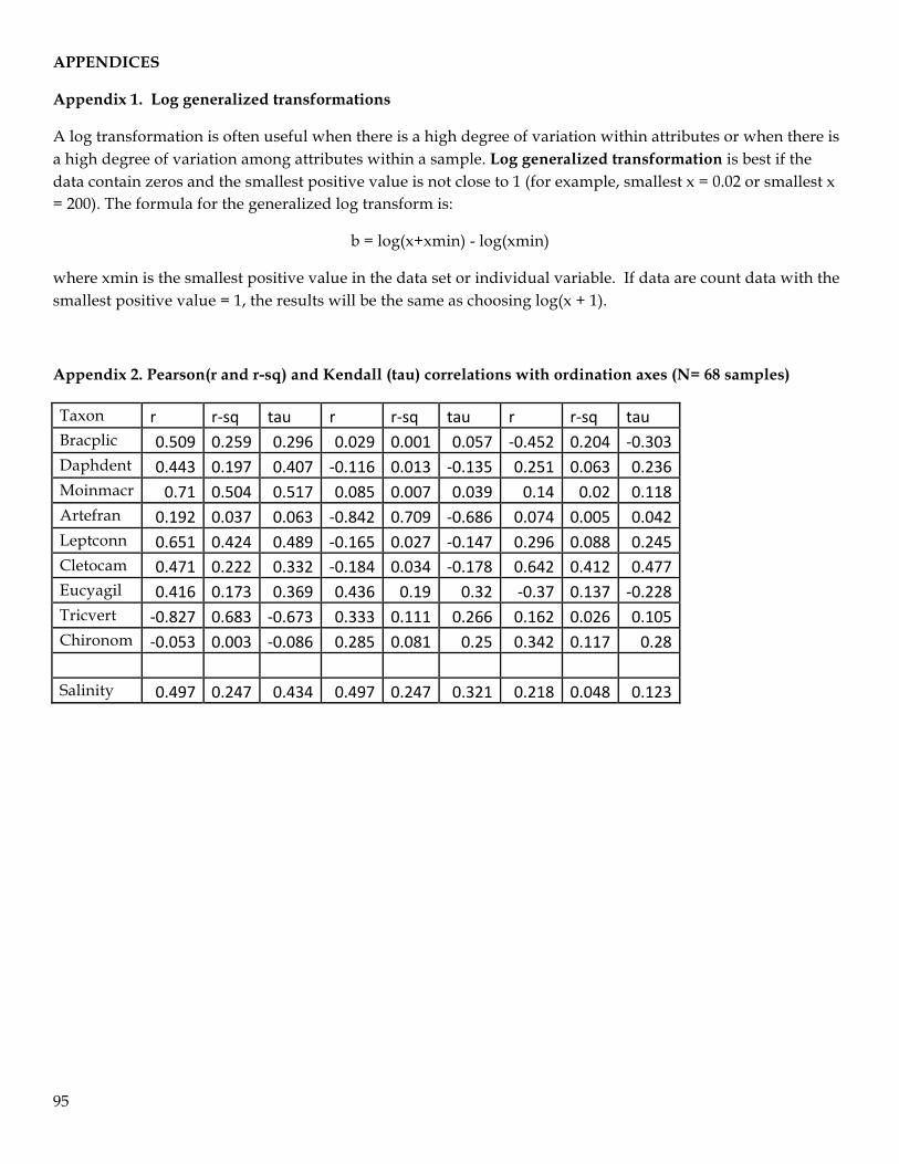
95
APPENDICES
Appendix 1. Log generalized transformations
A log transformation is often useful when there is a high degree of variation within attributes or when there is a high degree of variation among attributes within a sample. Log generalized transformation is best if the data contain zeros and the smallest positive value is not close to 1 (for example, smallest x = 0.02 or smallest x = 200). The formula for the generalized log transform is:
b = log(x+xmin) - log(xmin)
where xmin is the smallest positive value in the data set or individual variable. If data are count data with the smallest positive value = 1, the results will be the same as choosing log(x + 1).
Appendix 2. Pearson(r and r-sq) and Kendall (tau) correlations with ordination axes (N= 68 samples)
Taxon r r-‐sq tau r r-‐sq tau r r-‐sq tau Bracplic 0.509 0.259 0.296 0.029 0.001 0.057 -‐0.452 0.204 -‐0.303 Daphdent 0.443 0.197 0.407 -‐0.116 0.013 -‐0.135 0.251 0.063 0.236 Moinmacr 0.71 0.504 0.517 0.085 0.007 0.039 0.14 0.02 0.118 Artefran 0.192 0.037 0.063 -‐0.842 0.709 -‐0.686 0.074 0.005 0.042 Leptconn 0.651 0.424 0.489 -‐0.165 0.027 -‐0.147 0.296 0.088 0.245 Cletocam 0.471 0.222 0.332 -‐0.184 0.034 -‐0.178 0.642 0.412 0.477 Eucyagil 0.416 0.173 0.369 0.436 0.19 0.32 -‐0.37 0.137 -‐0.228 Tricvert -‐0.827 0.683 -‐0.673 0.333 0.111 0.266 0.162 0.026 0.105 Chironom -‐0.053 0.003 -‐0.086 0.285 0.081 0.25 0.342 0.117 0.28
Salinity 0.497 0.247 0.434 0.497 0.247 0.321 0.218 0.048 0.123
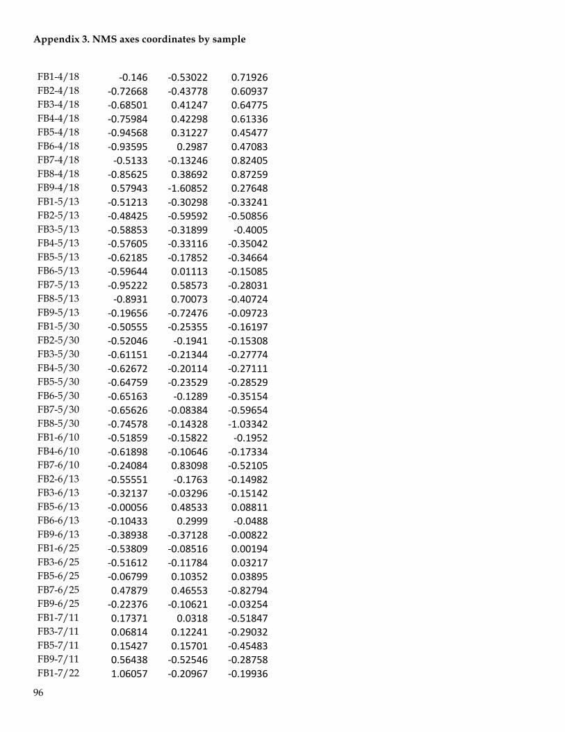
96
Appendix 3. NMS axes coordinates by sample FB1-4/18 -‐0.146 -‐0.53022 0.71926 FB2-4/18 -‐0.72668 -‐0.43778 0.60937 FB3-4/18 -‐0.68501 0.41247 0.64775 FB4-4/18 -‐0.75984 0.42298 0.61336 FB5-4/18 -‐0.94568 0.31227 0.45477 FB6-4/18 -‐0.93595 0.2987 0.47083 FB7-4/18 -‐0.5133 -‐0.13246 0.82405 FB8-4/18 -‐0.85625 0.38692 0.87259 FB9-4/18 0.57943 -‐1.60852 0.27648 FB1-5/13 -‐0.51213 -‐0.30298 -‐0.33241 FB2-5/13 -‐0.48425 -‐0.59592 -‐0.50856 FB3-5/13 -‐0.58853 -‐0.31899 -‐0.4005 FB4-5/13 -‐0.57605 -‐0.33116 -‐0.35042 FB5-5/13 -‐0.62185 -‐0.17852 -‐0.34664 FB6-5/13 -‐0.59644 0.01113 -‐0.15085 FB7-5/13 -‐0.95222 0.58573 -‐0.28031 FB8-5/13 -‐0.8931 0.70073 -‐0.40724 FB9-5/13 -‐0.19656 -‐0.72476 -‐0.09723 FB1-5/30 -‐0.50555 -‐0.25355 -‐0.16197 FB2-5/30 -‐0.52046 -‐0.1941 -‐0.15308 FB3-5/30 -‐0.61151 -‐0.21344 -‐0.27774 FB4-5/30 -‐0.62672 -‐0.20114 -‐0.27111 FB5-5/30 -‐0.64759 -‐0.23529 -‐0.28529 FB6-5/30 -‐0.65163 -‐0.1289 -‐0.35154 FB7-5/30 -‐0.65626 -‐0.08384 -‐0.59654 FB8-5/30 -‐0.74578 -‐0.14328 -‐1.03342 FB1-6/10 -‐0.51859 -‐0.15822 -‐0.1952 FB4-6/10 -‐0.61898 -‐0.10646 -‐0.17334 FB7-6/10 -‐0.24084 0.83098 -‐0.52105 FB2-6/13 -‐0.55551 -‐0.1763 -‐0.14982 FB3-6/13 -‐0.32137 -‐0.03296 -‐0.15142 FB5-6/13 -‐0.00056 0.48533 0.08811 FB6-6/13 -‐0.10433 0.2999 -‐0.0488 FB9-6/13 -‐0.38938 -‐0.37128 -‐0.00822 FB1-6/25 -‐0.53809 -‐0.08516 0.00194 FB3-6/25 -‐0.51612 -‐0.11784 0.03217 FB5-6/25 -‐0.06799 0.10352 0.03895 FB7-6/25 0.47879 0.46553 -‐0.82794 FB9-6/25 -‐0.22376 -‐0.10621 -‐0.03254 FB1-7/11 0.17371 0.0318 -‐0.51847 FB3-7/11 0.06814 0.12241 -‐0.29032 FB5-7/11 0.15427 0.15701 -‐0.45483 FB9-7/11 0.56438 -‐0.52546 -‐0.28758 FB1-7/22 1.06057 -‐0.20967 -‐0.19936
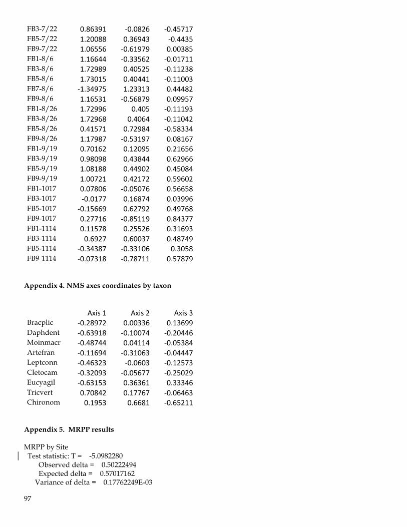
97
FB3-7/22 0.86391 -‐0.0826 -‐0.45717 FB5-7/22 1.20088 0.36943 -‐0.4435 FB9-7/22 1.06556 -‐0.61979 0.00385 FB1-8/6 1.16644 -‐0.33562 -‐0.01711 FB3-8/6 1.72989 0.40525 -‐0.11238 FB5-8/6 1.73015 0.40441 -‐0.11003 FB7-8/6 -‐1.34975 1.23313 0.44482 FB9-8/6 1.16531 -‐0.56879 0.09957 FB1-8/26 1.72996 0.405 -‐0.11193 FB3-8/26 1.72968 0.4064 -‐0.11042 FB5-8/26 0.41571 0.72984 -‐0.58334 FB9-8/26 1.17987 -‐0.53197 0.08167 FB1-9/19 0.70162 0.12095 0.21656 FB3-9/19 0.98098 0.43844 0.62966 FB5-9/19 1.08188 0.44902 0.45084 FB9-9/19 1.00721 0.42172 0.59602 FB1-1017 0.07806 -‐0.05076 0.56658 FB3-1017 -‐0.0177 0.16874 0.03996 FB5-1017 -‐0.15669 0.62792 0.49768 FB9-1017 0.27716 -‐0.85119 0.84377 FB1-1114 0.11578 0.25526 0.31693 FB3-1114 0.6927 0.60037 0.48749 FB5-1114 -‐0.34387 -‐0.33106 0.3058 FB9-1114 -‐0.07318 -‐0.78711 0.57879
Appendix 4. NMS axes coordinates by taxon Axis 1 Axis 2 Axis 3 Bracplic -‐0.28972 0.00336 0.13699 Daphdent -‐0.63918 -‐0.10074 -‐0.20446 Moinmacr -‐0.48744 0.04114 -‐0.05384 Artefran -‐0.11694 -‐0.31063 -‐0.04447 Leptconn -‐0.46323 -‐0.0603 -‐0.12573 Cletocam -‐0.32093 -‐0.05677 -‐0.25029 Eucyagil -‐0.63153 0.36361 0.33346 Tricvert 0.70842 0.17767 -‐0.06463 Chironom 0.1953 0.6681 -‐0.65211
Appendix 5. MRPP results MRPP by Site Test statistic: T = -5.0982280 Observed delta = 0.50222494 Expected delta = 0.57017162 Variance of delta = 0.17762249E-03
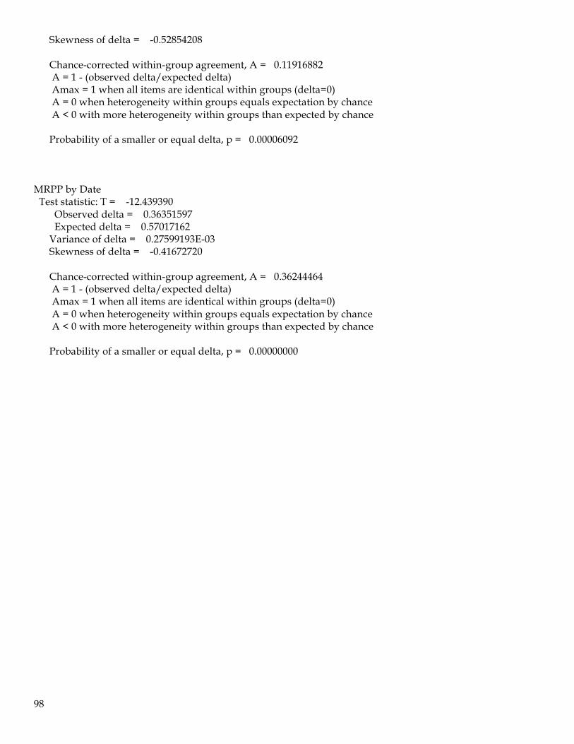
98
Skewness of delta = -0.52854208 Chance-corrected within-group agreement, A = 0.11916882 A = 1 - (observed delta/expected delta) Amax = 1 when all items are identical within groups (delta=0) A = 0 when heterogeneity within groups equals expectation by chance A < 0 with more heterogeneity within groups than expected by chance Probability of a smaller or equal delta, p = 0.00006092 MRPP by Date Test statistic: T = -12.439390 Observed delta = 0.36351597 Expected delta = 0.57017162 Variance of delta = 0.27599193E-03 Skewness of delta = -0.41672720 Chance-corrected within-group agreement, A = 0.36244464 A = 1 - (observed delta/expected delta) Amax = 1 when all items are identical within groups (delta=0) A = 0 when heterogeneity within groups equals expectation by chance A < 0 with more heterogeneity within groups than expected by chance Probability of a smaller or equal delta, p = 0.00000000
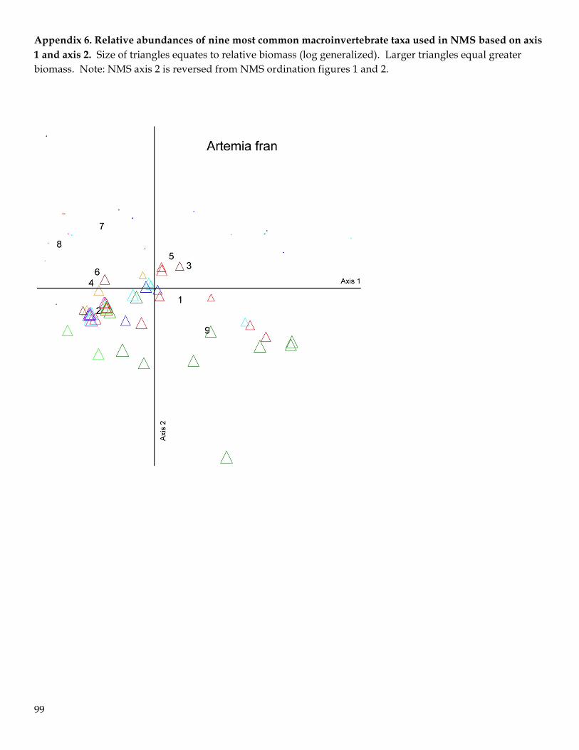
99
Appendix 6. Relative abundances of nine most common macroinvertebrate taxa used in NMS based on axis 1 and axis 2. Size of triangles equates to relative biomass (log generalized). Larger triangles equal greater biomass. Note: NMS axis 2 is reversed from NMS ordination figures 1 and 2.
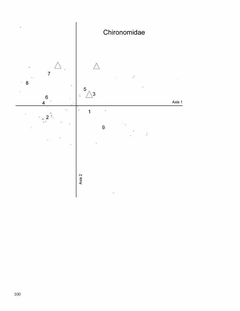
100
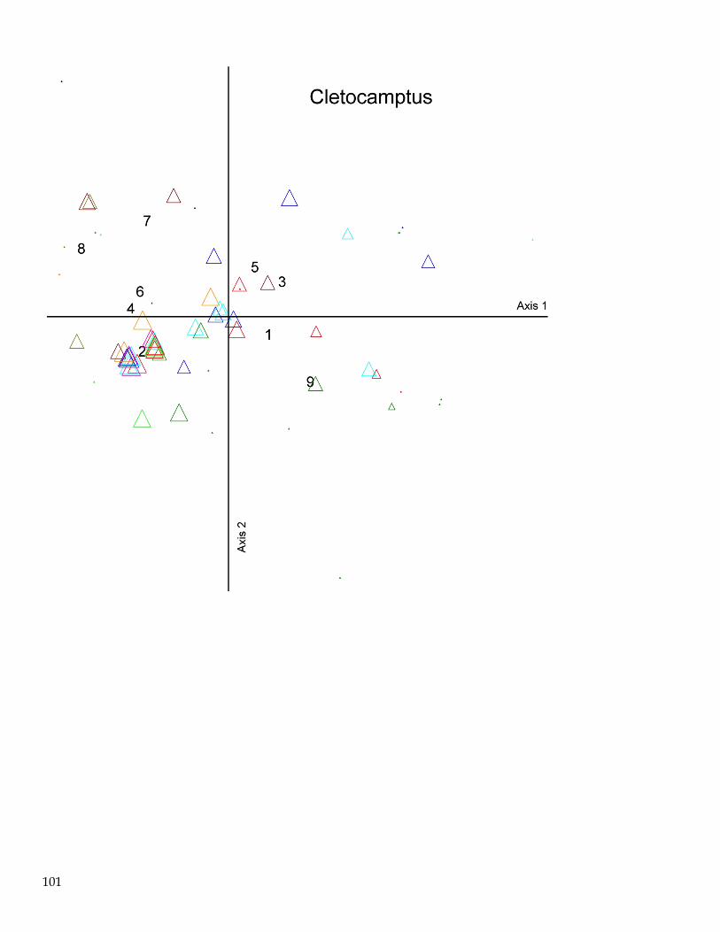
101
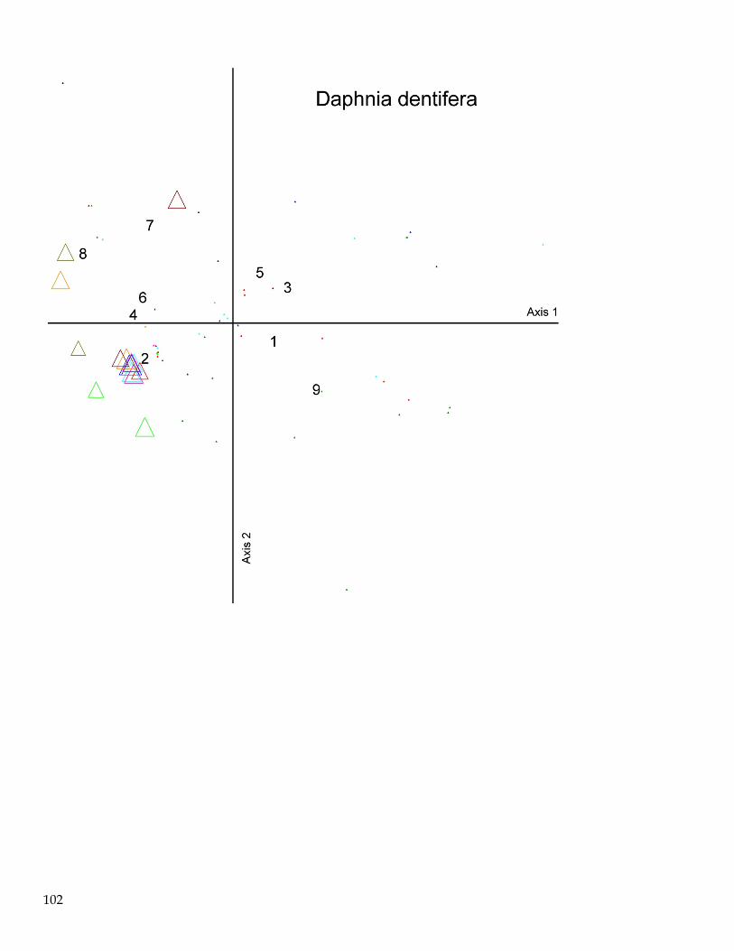
102
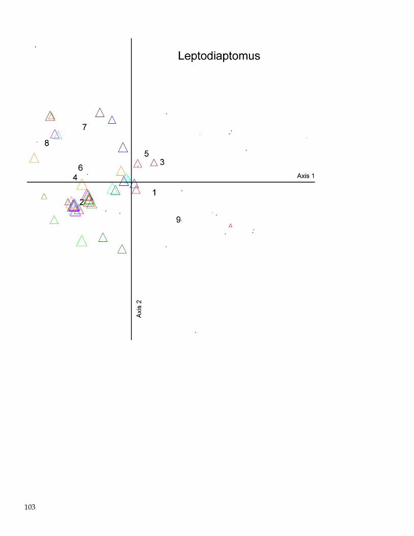
103
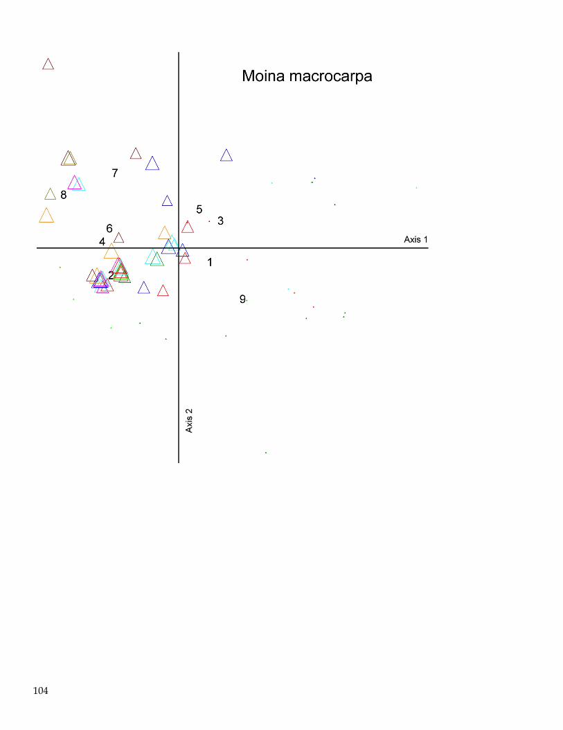
104
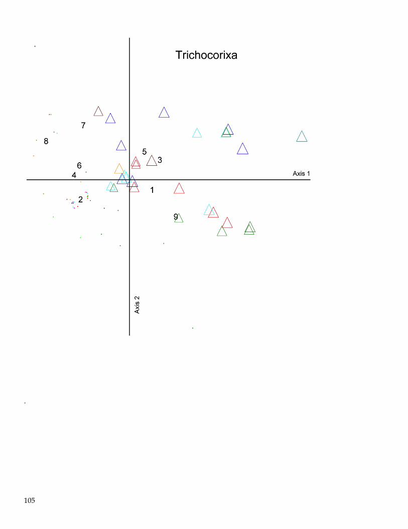
105
.