faculty of earth science and engineering petroleum and
TRANSCRIPT

University of Miskolc
Faculty of Earth Science and Engineering
Petroleum and Natural Gas Institute
DATA ANALYSIS AND SIMULATION OF
WATERFLOODING IN A CARBONATE
RESERVOIR
MSc Thesis in Petroleum Engineering
Author: Hamzah Salih Mahdi AL-Yasiri.
Supervisor: Bánki Dániel.
Miskolc, May 5, 2021

Thesis assignment
for
Hamza Salih Mahdi Al-Yasiri
Petroleum Engineering, MSc student
Title of the thesis work: Data analysis and simulation of waterflooding in a carbonate reservoir Tasks: Based on the given dataset briefly introduce the investigated field, and analyze the
production data, summarize the history of the fields operation Based on a literature review, summarize the basic reservoir engineering parameters and methods used in evaluation of waterflooding as a theoretical chapter of your study Choose a well-pattern on the given reservoir and apply a simulation for waterflooding, relying on the base rates and methods applied on the field during depletion. Analyze the results and give conclusion, pointing out future plans for optimizing and monitoring the waterflood.
Department supervisor: Daniel Banki, assistant lecturer
Dr. Zoltán Turzó
University Professor, Head of Department
05. May 2020., Miskolc
MISKOLCI EGYETEM
Műszaki Földtudományi Kar
Kőolaj és Földgáz Intézet
UNIVERSITY OF MISKOLC
Faculty of Earth Science & Engineering
Institute of Petroleum and Natural Gas
H3515 Miskolc, Egyetemváros, HUNGARY Tel: (36) 46 565 078
[email protected] www.kfgi.uni-miskolc.hu

Proof Sheet for thesis submission for Petroleum Engineering MSc students
Name of student: Hamza Salih Mahdi Al-Yasiri Neptune code: HV505G
Title of Thesis: Data analysis and simulation of waterflooding in a carbonate reservoir
Declaration of Originality I hereby certify that I am the sole author of this thesis and that no part of this thesis has been published or submitted for publication. I certify that, to the best of my knowledge, my thesis does not infringe upon anyone’s copyright nor violate any proprietary rights and that any ideas, techniques, quotations, or any other material from the work of other people included in my thesis, published or otherwise, are fully acknowledged in accordance with standard referencing practices. 5 May 2021
Signature of the student
Statement of the Department Advisor1
Undersigned agree/ do not agree to the submission of this
Thesis. 5 May 2021
Signature of
Department Advisor
The thesis has been submitted: Date
Administrator of Petroleum and Natural Gas Institute
1 Thesis can be submitted regardless of the consultant’s consent.

Acknowledgment
First and foremost, praise and thank God, the Almighty, for His showers of blessings
throughout my research work to complete the thesis.
I would like to express my extreme gratitude to my supervisor, Bánki Dániel, for his
invaluable advice, continuous support, and patience during this study. He showed me the
methodology to carry out the research and present the research works as clearly as possible.
It was a great privilege and honor to work and study under his guidance.
Besides my supervisor, I would like to thank my Co-supervisor: Abbas Radhi, for his
encouragement, insightful comments and make the data obtained applicable and tangible.
My sincere thanks go to Hatem Alamara, the friend and the teacher, for his dynamism,
vision, sincerity, and motivation have deeply inspired me in a reservoir engineering subject.
His teaching skills were remarkable during the material balance subject, equipping us with
all information needed to be a professional reservoir engineer. Also, I would like to thank
him for his friendship, empathy, and great sense of humor.
Furthermore, I would like to give unique and great thanks to my professor’s Dr. Gábor
Takács and Zoltán Turzó, for giving me great courses of production and artificial lift
methods.
My gratitude extends to Missan oil company (MOC), field operation division, reservoir,
and geology department for their support and for providing me with all necessary tools to
accomplish this study.
Finally, my sincere thanks go to Hasanain Al Saheib for his support and guidance to
accomplish realistic reservoir simulation

Dedication
I dedicate my thesis work to my family. A special feeling of gratitude to my loving parents,
Salih Mahdi and Khawlah Mohammed Ali, whose words of encouragement and push for
tenacity ring in my ears. My beloved brothers and sisters, particularly my brothers who have
never left my side.
To My friends who encourage and support me and all the people in my life who touch my
heart, I dedicate this research.

If we knew what it was we were doing,
it would not be called research, would it?
Albert Einstein

Contents 1 Chapter One: Introduction ............................................................................................. 1
1.1 Water Flooding Overview ...................................................................................... 2
1.2 Research Objectives ................................................................................................ 3
1.3 Research Methodology ........................................................................................... 3
1.4 Thesis Outlines ....................................................................................................... 4
2 Chapter Two: Theory..................................................................................................... 5
2.1 Interfacial Tension (IFT) ........................................................................................ 5
2.2 Wettability .............................................................................................................. 6
2.3 Capillary Pressure (Pc) ............................................................................................ 7
2.3.1 Hysteresis-Drainage......................................................................................... 9
2.3.2 Hysteresis-Imbibition .................................................................................... 10
2.4 Gravity Effect ....................................................................................................... 12
2.5 Relative Permeabilities ......................................................................................... 12
2.3.3 Hysteresis ...................................................................................................... 13
2.3.4 Absolute Permeability ................................................................................... 15
2.3.5 Wettability ..................................................................................................... 15
2.3.6 Interfacial Tension (IFT) ............................................................................... 16
2.6 Mobility Ratio ....................................................................................................... 17
2.7 Heterogeneity ........................................................................................................ 18
2.8 Buckley and Leverett Theory (1D FLOW) ........................................................... 19
2.8.1 Fractional Flow .............................................................................................. 19
2.8.2 Front Advance Equation ................................................................................ 20
2.9 Displacement Efficiency ....................................................................................... 22
2.10 Areal Sweep Efficiency (Ea) ............................................................................. 22
2.11 Wells Pattern ..................................................................................................... 23
2.12 Injectivity .......................................................................................................... 23

2.13 Vertical Sweep Efficiency ................................................................................. 25
2.14 Residual Oil Saturation (Sor) ............................................................................. 25
3 Chapter Three: The Development History Of Water Flooding ................................... 27
3.7 One-Dimensional Flow Studies ............................................................................ 27
3.8 Areal Sweep Efficiency (2D) ................................................................................ 28
3.8.1 Areal Sweep Prediction Methods .................................................................. 29
3.9 Vertical Sweep Efficiency Studies ....................................................................... 32
3.10 Waterflooding Surveillance............................................................................... 34
3.10.1 Hall Plot ......................................................................................................... 34
3.10.2 Hearn Plot ...................................................................................................... 36
3.10.3 Decline Curve (DC) ....................................................................................... 37
4 Chapter Four: Simulation and Production Data Analysis ........................................... 40
4.1 The Study Sector of Nine-Spot Pattern. ................................................................ 44
4.2 Primary and Secondary Formation Pressure Maintenance Analysis. ................... 46
4.3 Primary and Secondary Material Balance Calculations........................................ 50
4.4 Primary and Secondary Production Data Analysis. .............................................. 53
4.5 Injector Data Analysis .......................................................................................... 59
4.6 Simulation Sector Modelling ................................................................................ 62
4.6.1 History strategy: ............................................................................................ 65
4.6.2 Prediction Strategy ........................................................................................ 67
5 Chapter Five: Conclusion And Recommendations ..................................................... 74
5.7 Conclusion and Recommendation. ....................................................................... 74
5.8 Recommendation for Future Work ....................................................................... 75
6 Bibliography ................................................................................................................ 76
A. Appendix A ................................................................................................................. 81
B. Appendix B .................................................................................................................. 96
C. Appendix C ................................................................................................................ 101

D. Appendix D ............................................................................................................... 106
E. Appendix E ................................................................................................................ 117
List of Figures
Figure 1-1. Recovery methods. ............................................................................................. 1
Figure 1-2. Energy plot .......................................................................................................... 2
Figure 1-3. A. Waterflooding. B. Water injection. ................................................................ 3
Figure 2-1. Effect of interfacial tension on the nonwetting’ s displacement by a wetting liquid
............................................................................................................................................... 5
Figure 2-2. Force of Young’s equation in the water-wet system. ......................................... 6
Figure 2-3. Wettability effect ................................................................................................ 7
Figure 2-4. Capillary pressure in the water-wet system. ....................................................... 8
Figure 2-5. The effect of absolute permeability on the capillary pressure curve .................. 9
Figure 2-6. Drainage process ............................................................................................... 10
Figure 2-7. Imbibition process ............................................................................................ 11
Figure 2-8. Capillary pressure hysteresis sequence ............................................................. 11
Figure 2-9. Flooding performance in a dipping reservoir; (a) stable (b) stable (c) unstable12
Figure 2-10. Relative permeability of the drainage process. ............................................... 14
Figure 2-11. Relative permeability of the imbibition process. ............................................ 14
Figure 2-12. A. Photomicrograph and water/oil relative permeability curve for sandstone
containing large, well-connected pores. B. Photomicrograph and water/oil relative
permeability curve for sandstone containing tiny well-connected pores ............................ 15
Figure 2-13. Relative permeabilities for a range of wetting conditions (indicated by contact
angle) ................................................................................................................................... 16
Figure 2-14. Relative permeability curve after reducing the IFT ........................................ 17
Figure 2-15. A. Water has a viscosity higher than oil; B. Water has a viscosity less than oil.
............................................................................................................................................. 17
Figure 2-16. Mobility ratio with time. ................................................................................. 18
Figure 2-17. Characterization of reservoir heterogeneity depends on the Dykstra-Parsons
coefficient ............................................................................................................................ 19
Figure 2-18. The effect of oil viscosity (mobility ratio) on the fractional curve and the frontal
shape. ................................................................................................................................... 20
Figure 2-19. Water saturation distribution with location and time. .................................... 21
Figure 2-20. X-ray shadowgraphs of flood progress in scaled five-spot patterns ............... 22
Figure 2-21. Areal sweep efficiency at breakthrough ......................................................... 23
Figure 2-22. Conductance ratio curve ................................................................................. 24
Figure 3-1. Dykstra and Parson correlation ......................................................................... 32
Figure 3-2. EV versus the correlating parameter Y .............................................................. 33
Figure 3-3. Typical Hall plot for various conditions ........................................................... 35
Figure 3-4. Hearn plot illustrating interpretations of various slope changes ...................... 37
Figure 3-5. Classification of production decline curves ...................................................... 38
Figure 4-1. Reservoir layer distribution. ............................................................................. 40
Figure 4-2. Reservoir thickness of zone/sub-zone. ............................................................. 41
Figure 4-3. NTG of zones/sub-zones. .................................................................................. 41
Figure 4-4. Net oil thickness of zones/sub-zones. ............................................................... 42
Figure 4-5. MB21 sublayers. ............................................................................................... 43
Figure 4-6. Pressure gradient for several wells in the field. ................................................ 43
Figure 4-7. Invert nine-spot pattern of Well-36 (The study Sector). ................................... 44
Figure 4-8. Pressure variation diagram of the whole reservoir. .......................................... 46
Figure 4-9. Pressure variation diagram of the Sector (the invert nine-spot pattern). .......... 46
Figure 4-10. A. Dake Plot. B. Campbell plot ...................................................................... 47
Figure 4-11. Diagnostic plot for the sector .......................................................................... 48
Figure 4-12. Natural energy classification evaluation chart of the whole reservoir. ........... 49
Figure 4-13. Natural energy classification evaluation chart of the sector. .......................... 49
Figure 4-14. Havlena and Odeh model for the sector.......................................................... 51
Figure 4-15. Energy plot for the sector. .............................................................................. 52
Figure 4-16. The sector production rate Performance. ........................................................ 53
Figure 4-17. Cumulative production, oil rate, and water rate for the sector. ...................... 54
Figure 4-18. Stacked cumulative oil and water production for the sector. .......................... 54
Figure 4-19. The natural decline curve of oil wells of the sector. ....................................... 55
Figure 4-20. A plot of the daily oil rate for each well within the sector. ............................ 56
Figure 4-21. Sector wells cumulative oil rate. ..................................................................... 56
Figure 4-22. Decline curve result for the sector after the waterflooding. ........................... 57
Figure 4-23. Sector bubble map of 2021. ............................................................................ 57
Figure 4-24. Sector bubble map before water injection in Oct 2017. ................................. 58
Figure 4-25. Instantaneous and cumulative voidage replacement and cumulative liquid and
oil for the sector. .................................................................................................................. 59

Figure 4-26. Injection performance of Well-36................................................................... 60
Figure 4-27. Hall plot and bottom hole pressure. ................................................................ 60
Figure 4-28. Hearn and Hall plots. ...................................................................................... 61
Figure 4-29. Hall plot straight line post-fill-up. .................................................................. 61
Figure 4-30. A. Vertical permeability B. Horizontal permeability distribution for the field
model. .................................................................................................................................. 63
Figure 4-31. Porosity distribution for the field model. ........................................................ 63
Figure 4-32. Initial water saturation distribution for the field model. ................................. 64
Figure 4-33. The sector model chosen region and the wells. .............................................. 64
Figure 4-34. A. Initial oil saturation B. Oil saturation at the end of 2018........................... 65
Figure 4-35. Oil saturation and bubble map for the sector. ................................................. 66
Figure 4-36. Well-69H location for A. Full-field water saturation distribution B. Full-field
permeability distribution. .................................................................................................... 66
Figure 4-37. Cross-section slice for the injector (Well-36) of A. Oil saturation before the
water flooding. B. Oil saturation after the water flooding till the end of 2018. .................. 67
Figure 4-38. Predicted oil saturation in 2040. ..................................................................... 68
Figure 4-39. Cross-section slice for the injector (Well-36) of predicted oil saturation after
the water flooding in 2040. .................................................................................................. 68
Figure 4-40. The plot of sector oil rate, injection rate, and water cut with time. ................ 69
Figure 4-41. Sector remaining oil and reservoir. ................................................................. 69
Figure 4-42. Prediction cumulative oil and liquid for the sector model. ............................. 70
Figure 4-43. Predicted bubble map for the sector model in 2040. ...................................... 70
Figure 4-44. Ap1 simulation production performance. ....................................................... 71
Figure 4-45. Ap2 simulation Production Performance. ....................................................... 72
Figure 4-46. Well-47 simulation injection performance. .................................................... 72
Figure 4-47. Well-47 Simulation Production Performance. ................................................ 73
Figure A-1. Fractional flow curve and the slope. ................................................................ 86
Figure A-2. Saturation distribution with distance and the solution of the shock front........ 86
Figure C-1. DC result for the period 2012-2013. .............................................................. 101
Figure C-2. DC result for the period 2013-2014. .............................................................. 102
Figure C-3. DC result for the period 2014-2015. .............................................................. 102
Figure C-4. DC result for the period 2015-2016. .............................................................. 103
Figure C-5. DC result for the period Jan-2016 till Jun-2016............................................. 103
Figure C-6. DC result for the period 2016 jun-2017. ........................................................ 104

Figure C-7. DC result for the period 2017-2018. .............................................................. 104
Figure C-8. DC result for the period 2018-current. ........................................................... 105
Figure D-1. MB21 formation tops for the study field. ...................................................... 106
Figure D-2. Wellhead pressure map for the sector. ........................................................... 107
Figure D-3. Well-6 cumulative oil, oil rate, and water rate. .............................................. 107
Figure D-4. Well-6 production performance curves. ........................................................ 108
Figure D-5. Well-15 cumulative oil, oil rate, and water rate............................................. 108
Figure D-6. Well-15 production performance curves. ...................................................... 109
Figure D-7. Well-16 cumulative oil, oil rate, and water rate............................................. 109
Figure D-8. Well-16 production performance curves. ...................................................... 110
Figure D-9. Well-47 cumulative oil, oil rate, and water rate............................................. 110
Figure D-10. Well-47 production performance curves. .................................................... 111
Figure D-11. Well-50 cumulative oil, oil rate, and water rate........................................... 111
Figure D-12. Well-50 production performance curves. .................................................... 112
Figure D-13. Well-53 cumulative oil, oil rate, and water rate........................................... 112
Figure D-14. Well-53 production performance curves. .................................................... 113
Figure D-15. Well-69H cumulative oil, oil rate, and water rate. ....................................... 113
Figure D-16. Well-69H production performance curves. ................................................. 114
Figure D-17. Well-116 cumulative oil, oil rate, and water rate......................................... 114
Figure D-18. Well-116 production performance curves. .................................................. 115
Figure D-19. Well-36 cumulative oil, oil rate, and water rate........................................... 115
Figure D-20. Well-36 production performance curves. ................................................... 116
Figure D-21. Well-36 schematic. ...................................................................................... 116
Figure E-1. Well-116 simulation production performance. .............................................. 117
Figure E-2. Well-15 simulation production performance. ................................................ 117
Figure E-3. Well-16 simulation production performance. ................................................ 118
Figure E-4. Well-6s simulation production performance. ................................................. 118
Figure E-5. Well-50 simulation production performance. ................................................ 119
Figure E-6. Well-53 simulation production performance. ................................................ 119
Figure E-7. Well-69H simulation production performance............................................... 120
Figure E-8. Well-36 injection production performance. ................................................... 120
Figure E-9. Field simulation production rate. ................................................................... 121

List of Tables
Table 3-1. Traditional decline analysis: governing equations and characteristic linear Plots.
............................................................................................................................................. 39
Table 4-1. The wells of the study sector. ............................................................................. 45
Table 4-2. Appraisal Wells. ................................................................................................. 71
Table B-1. The history of waterflooding Models. ............................................................... 96
Table B-2. Fassihi non-linear regression coefficients. ........................................................ 98
Table B-3. The front advance equations. ............................................................................. 98
Table B-4. Material balance results. ................................................................................... 99
Table C-1. Decline curve wells number ........................................................................... 101

Nomenclatures
Latin letters:
Gas formation volume factor, [rcf/scf]
Formation compressibility, [sip]
Effective total compressibility, [sip]
Water compressibility, [sip]
Absolute permeability, [md]
Cumulative oil produced, [STB]
Pressure, [psi]
Average reservoir pressure, [psi]
Flowing bottom hole pressure, [psi]
Flow rate, [STB/day], [scf/d=scfd]
Capillary radius, [m], [nm]
Temperature, [C], [F]
Time, [day]
DI Energy indices [-]
Pb Bubble point pressure [psi]
API American petroleum institute oil density
IFT Interfacial tension [dyne/cm]
WOR Water oil ratio [-]
PC Capillary pressure [psi]
The interfacial tension between oil and rock [dyne/cm]
The interfacial tension between oil and water [dyne/cm]
𝜎𝑤𝑠 The interfacial tension between water and rock [dyne/cm]
Contact angel between the immiscible fluids
Po Oil pressure [psi]
Oil pressure at the contact between oil and water [psi]
Water pressure at the contact between oil and water [psi]
Water pressure [psi]
h Hight [ft]
Sw Water saturation [-]
So Oil saturation [-]

Swc Critical water saturation [-]
Swi Irreducible water saturation [-]
Sor Residual oil saturation [-]
Snw Nonwetting phase saturation [-]
Soc Critical oil saturation [-]
Waterfront saturation [-]
Average water saturation behind the front before the breakthrough [-]
Average water saturation behind the front after the breakthrough [-]
OOIP Original oil in place [STB]
Pd Displacement pressure [psi]
Injection rate [STB/d]
Water effective permeability [md]
Oil effective permeability [md]
Dake gravity segregation coefficient
Corey coefficient
Water relative permeability [md]
Oil relative permeability [md]
Relative permeability at 50% of the permeability probability [md]
Relative permeability at 84.1% of the permeability probability [md]
Total liquid flow rate [bbl/d]
Dykstra-Parsons coefficient
Water flow rate [bbl/d]
Water fraction (Water cut) [-]
M Mobility ratio [-]
The percentage of the water injected from the pore volume at the breakthrough [-]
The percentage of the water injected from the pore volume after the breakthrough [-]
Cumulative injected water at the breakthrough [STB]
Time of the breakthrough
Cumulative injected water after the breakthrough [STB]
Vrp Voidage replacement ratio [-]
Injected water invasion radius [ft]
The pressure difference [psi]

𝐵𝑤 Water formation volume factor [bbl/STB]
𝐵𝑜 Oil formation volume factor [bbl/STB]
Displacement efficiency [-]
𝐸𝐴 Areal sweep efficiency [-]
𝐸𝑉 Vertical sweep efficiency [-]
Recovery factor [-]
Capillary number [-]
Liquid velocity (oil or water) [ft/s]
Electrical resistivity [Ohm]
Voltage difference [volt]
I Current, electric [amper]
Areal sweep efficiency at the breakthrough [-]
Cumulative oil produced at the breakthrough, [STB]
injection bottom hole flowing pressure [psi]
Injectivity index [Bbl/d/psi]
Skin factor [-]
Boundary radius, external [ft]
D The decline rate of the decline curve [-]
Hyperbolic function [-]
NTG Net to gross
RFT Repeat formation tester
MDT Modular formation dynamics tester
𝑁𝑝𝑟 The elastic production ratio [-]
𝐵𝑜𝑖 Intail oil formation volume factor [bbl/STB]
𝑃𝑖 Initial pressure [psi]
𝐷𝑝𝑟 Formation pressure decline corresponding to 1% OOIP recovery [psi]
𝐹 Material balance total withdrawal [bbl]
𝐸𝑜 Oil expansion
𝐸𝑓𝑤 Rock and connate water expansion
𝑁 Initial oil in place [STB]
𝑊𝑒 Cumulative water influx (encroachment) [STB]
𝑅𝑝 Cumulative gas-oil ratio [Scf/STB]

𝑅𝑠𝑖 Initial Gas solubility in oil [rcf/bbl]
𝐵 Aquifer constant [STB/psi]
𝐷𝐷𝐼 Oil and gas expansion energy index [-]
𝐸𝐷𝐼 Rock and connate water expansion energy index [-]
𝑊𝐼𝐷𝐼 The pot aquifer and the water injection index [-]
DC Decline curve
HI Hall plot index
TVD True vertical depth [ft]
MD Measured depth [ft]
Liquid mass [lb mass]
Reservoir water volume [bbl]
Bulk volume [ft3]
Length [ft]
Front saturation distance [ft]
Wp Cumulative produced water [STB]
Ei (x) exponential integral
pe external boundary pressure [psi]
Greek letters:
Liquid mobility [mD/cP]
Oil viscosity [cP]
Porosity, [-]
Water density [lb/cf]
Oil density [lb/cf]
Water viscosity [cP]

1
1 CHAPTER ONE: INTRODUCTION
Reservoir oil has an original mechanism that pushes the oil to the surface; it could be a very
strong mechanism that allows achieving a high recovery factor or a weak mechanism that
achieves low recovery. There will be residual oil in the reservoir in both cases, and those
natural mechanisms called the primary recovery, and to extract that residual oil, a secondary
recovery needs to be imposed in the reservoir. The secondary recovery methods are water
flooding and immiscible gas injection, and it aims to sweep as much oil as possible to
improve the recovery and provide pressure maintenance. There is always an oil left behind
after the secondary recovery; therefore, a hundred percent of the recovery factor is
unpractically achieved by primary and secondary recovery methods. The displaced fluid (oil)
will separate from the continuous liquid and congregate as immobile discontinuous residual
oil. It needs special treatment like the enhanced oil recovery (EOR) to extract it. Enhanced
oil recovery methods like miscible gas injection, thermal methods like steam injection, and
chemical methods like injecting low concentrations of chemicals, surfactants, and polymers
dissolved in water (ASP = alkaline, surfactant, polymer) (Warner, 2015) (See Figure 1-1).
Undersaturated reservoirs with pressure much higher than the bubble point (Pb) suffered
from a lack of sufficient energy. In this type of reservoirs, the primary (natural) energy is the
expansion of oil, connate water, and rocks. Water flooding in an early time is a suitable
investment in this kind of reservoirs, and in this case, it is no more secondary recovery and
can be considered a primary recovery because of the implementation time. Primary recovery
for undersaturated reservoirs is slight <5% OOIP, and water flooding can increase the
recovery in this kind of reservoir. In the reservoir with gas cap drives, the primary recovery
is 40-60%. In a reservoir with a very strong water drive, the primary recovery is very efficient
and can achieve pressure maintenance.
Figure 1-1. Recovery methods.
Reservoir
flow rate
Time

2
1.1 WATER FLOODING OVERVIEW
Water flooding represents injecting water into the reservoir to stabilize the pressure by
achieving a steady-state flow at which the mass-in equals mass-out and sweep the oil to
improve the recovery. At this stage, the predominant drive is the water flooding because all
other expansions, the natural mechanisms like the gas cap, solution gas drive, rock
expansion, and water influx, depend on the pressure drop (see Figure 1-2) therefore
achieving pressure maintenance by water flooding will theoretically reduce the pressure drop
to zero. Water flooding has accidentally proved since 1880, increasing the oil recovery, and
there was no water flooding application until 1930, when many injection projects started.
Many recovery methods have developed in the past years, but among these methods, water
flooding is the most efficient, and more than half of oil globally is obtained by waterflooding
for the following reasons (Mogollón, 2017) (Craig, 1971) :
A. Availability of water.
B. Water treatment and injection plant facilities are relatively lower cost than other
methods.
C. The efficiency of the water to spread and displace oil.
Figure 1-2. Energy plot
[Modified after (Alamara, 2020)]
Water flooding usually refers to injecting water into the oil pay zone; therefore, it is efficient
if there are barriers between the pay zone sublayers as a noncommunicating layered reservoir
(stratified). Some literature mentioned a water injection technique, which refers to injecting
water into the aquifer, which is practically unacceptable because of the high cost of drilling
DI
time
Gas cap expansion
Water flooding

3
well deep into the aquifer, and if there are barriers, this technique is not preferable (See
Figure 1-3).
Figure 1-3. A. Waterflooding. B. Water injection.
1.2 RESEARCH OBJECTIVES
This research aims to study the waterflooding performance in flooded undersaturated
carbonate oil reservoirs when the waterflooding already started. To reveal the necessity of
waterflooding, point out the waterflooding drive index contribution to the energy plot and
simulate the field to get the complete picture of the process and recommend the necessary
action needed to calibrate the injection and meet more or less the ideal waterflooding process.
1.3 RESEARCH METHODOLOGY
To evaluate and calibrate the waterflooding performance in the flooded undersaturated
carbonate oil reservoir and showing the necessity of the secondary recovery, the following
has been used:
• Apply material balance diagnostic plot to identify the drive mechanism before and
after waterflooding using Dack plot, Campbell plot, and Li and Zhu chart.
• Apply the material balance equation to calculate the original oil in place and draw
the energy plot before and after waterflooding using Havlena and Odeh method.
Unite B
Injector well Producer well
Unite C
Unite A
Aquifer
Reservoir
Aquifer
Injector well Producer well
A
B

4
• Apply production data analysis before and after waterflooding: using decline curve
analysis, checking the oil rate and cumulative performance, analyzing the single well
performance, obtain the bubble map and calculate the voidage replacement ratio.
• Apply injector data analysis using Hall plot and Hearn plot.
• Apply numerical simulation using sector model.
1.4 THESIS OUTLINES
Chapter1 gives an introduction to the recovery methods and waterflooding. Chapter2
represents the theory behind waterflooding and points out all the factors affecting
waterflooding. Chapter 3 contains the literature review of waterflooding. Chapter 4 is the
practical part where the sector model is used to analyze the waterflooding. Chapter 5
represents the discussion and the recommendation. Appendix A contains some essential
derivation of Buckley and Leverett displacement equations, Welge graphic front equation,
and areal sweep efficiency. Appendix B contains the tables. Appendix C includes the decline
curve analysis figures for every single well. Appendix D includes the daily production and
cumulative performance for each single wells. Appendix E contains the simulation result
for each single wells.

5
2 CHAPTER TWO: THEORY
2.1 INTERFACIAL TENSION (IFT)
Interfacial tension is the region of limited solubility where two immiscible liquids get in
contact or the work that must be done to increase the contact area by one unit (Willhite,
1986). When water and oil, immiscible, displaced, they will not mix, and surface tension
will develop between them because of the same molecules’ cohesive forces. The center
molecules are in an equilibrium state due to the cohesion force being equal in all directions
where similar molecules present. The molecules in liquid-liquid contact are not identical in
size; therefore, the molecules’ force is an imbalance. The highest force is toward the center,
where the same molecules impose interfacial tension in the contact. The interfacial tension
is essential in water flooding due to its importance as an input variable into two calculations,
OOIP calculation, because it is essential in the Pc vs. Sw graph and the fractional flow
calculation when the capillary is counted. With the two immiscible fluids flowing in the
porous media, an adhesive force will impose between the liquids and the media’s grain. The
forces’ equation is defined by Young’s equation (See Figure 2-2). The decrease of IFT
increases the relative permeability for both liquids, the displaced and the displacing fluids,
making the two liquids miscible (See Figure 2-1). IFT can be measured by simply a piece of
metal submerged in the liquid then measuring the force imposed on the plate’s wall.
Figure 2-1. Effect of interfacial tension on the nonwetting’ s displacement by a wetting
liquid
(Necmettin, 1966).

6
2.2 WETTABILITY
Wettability is the propensity of a liquid to spread on the rock surface with other liquid
presence. If the contact angle between water and oil less than 90o, the rock is water wet
(hydrophilic), and the water spreads on the rock surface where the small porous while the oil
locates in the larger porous. If the contact greater than 90o, the rock is oil-wet (hydrophobic).
Mixed-wet (Dalmatian), the rocks are oil and water wet in different reservoir locations, or
the tiny pores are water-wet while the large pores are oil-wet. Equation (2.1) is the Young
equation representing the equilibrium of the interfacial tension forces; the only measurable
thing in the equation is the contact angle, which is one of the methods to determine the
reservoir rocks’ wettability. The other methods to determine the wettability are Amott,
USBM, and Amott Harvey, which use the displacement laboratory data.
(2.1)
Figure 2-2. Force of Young’s equation in the water-wet system.
The reservoir is initially water wet, but hydrocarbon is a very complex mixture containing
many components that could be adsorbed by the rock or precipitate on the rock, altering the
wettability of the rock to oil-wet; for instance, the resin and asphaltene molecules’ presence
can alter the wettability to oil-wet because the rock grains adsorb these molecules and form
a film on the grains. Maintaining the reservoir pressure above the upper asphaltene envelop
and keeping the balance between the aromatic and asphaltene oil components is good
practice for preventing asphaltene precipitation in the reservoir. In the oil industry,
wettability is a qualitative term, and it does not input in all calculations. The wettability has
a strength range from strong, moderate to weak wettability. Wettability affects the recovery
of water flooding; the water-wet recovery factor higher than the oil-wet recovery factor by
Oil
Solid 𝝈𝒐𝒔
𝝈𝒘𝒔
Water

7
15%. Craig stated that “in a preferentially water-wet system, the oil is recovered at a lower
WOR and consequently with less injected water than in an oil-wet system” (Craig, 1971).
As shown in Figure 2-3, the relationship between recovery and injected volume is linearly
(proportional); however, at a certain point, the slope decreases where the breakthrough
happened. After this point, more injected volume is required to achieve a low recovery
factory; then, the curve becomes horizontal and not a function of injected volume, which
means all recoverable volume of oil has been extracted; therefore, the recovery factor is
constant. The recovery period after the breakthrough till the point of no recovery ( where the
curve became horizontal with zero slopes) for the oil-wet system is more extended than the
water-wet system, as shown by a shaded area. Experiments on mixed wet system cores
(Salathiel, 1973) concluded that a mixed wet system could achieve a very low residual oil
and high recovery factor because water remains in the small water-wet porous, while oil still
flows more readily through the large oil-wet pores
Figure 2-3. Wettability effect
[Modified after (Owens, 1971)].
2.3 CAPILLARY PRESSURE (PC)
Capillary pressure raises the liquid in a capillary tube in the presence of other fluid where
liquid-liquid and liquid-solid interfacial tension imposed in the contact. It can be calculated
and identify simply by the nonwetting pressure minus the wetting pressure. However, in the

8
oil industry, capillary pressure is obtained by oil pressure minus water pressure regardless
of wettability type; therefore, Pc is positive for water wet and negative for oil-wet since the
nonwetting pressure always greater than the wetting pressure. A large diameter tube yields
a large radius of curvature, so the contact between the phases is flat; therefore, the phases’
pressures at the interface are equal, so Pc is zero. If the diameter is small, the curvature radius
is tiny; interfacial tension is imposed by the preferential wetting of the rock for one phase
causing a measurable pressure difference in the contact between the fluids.
Figure 2-4. Capillary pressure in the water-wet system.
The following formulas (Equation (2.2)) are obtained for the water-wet system that drives
from the free body and the capillary tube shown in Figure 2-4. And it represents the capillary
pressure during the static condition ( after the migration ); therefore its necessary to distribute
the saturation at the initialization stage.
(2.2)
In the dynamic stage when the fluid flow, the real reservoir geometry is very complicated
than a standard tube; many curvature forms when the fluid flows; therefore, equation (2.2)
is no more representing the reservoir capillary when the fluids are flowing; therefore, another
formula is necessary to account for the effect of different curvatures in the dynamic stage as
in equation (2.3).
(2.3)
Pc is an essential tool for reservoir engineers obtained in the laboratory from several test
methods as a function of the saturation that results in two curves: drainage and imbibition.
Oil
Water
Po
Pw
Oil
Water

9
The drainage curve represents the displacement of the wetting phase by the nonwetting
phase, which is vital for OOIP calculation because it plays the primary role of liquids’ (water
and oil) distribution above the oil-water contact (OWC). The imbibition curve displacement
of the nonwetting phase by the wetting phase and its importance in the fractional flow
calculations besides the drainage curve. The permeability controls the height of the transition
zone; high permeability yields the following:
1. Less transition zone than low permeability because the grains are well-sorted and
rounded, and there is no clay presence so that the fluid rises to the same height.
2. The higher permeability available and the more well-sorted grains, the lower the
connate water in the reservoir (see Figure 2-5).
3. Lower displacement pressure (Pd) is required for the nonwetting phase to push
(displace) the wetting phase (drainage process).
Figure 2-5. The effect of absolute permeability on the capillary pressure curve
[Modified after (Ahmed, 2018)].
2.3.1 HYSTERESIS-DRAINAGE
The drainage process identifies as the displacing of the wetting phase by the nonwetting
phase if the pressure exceeds the displacement pressure. Drainage needs more capillary
pressure than the imbibition process. At the start, low capillary pressure is required because
the nonwetting phase invades the bigger diameter first, where the curvature is slight, and the
curvature radius is significant, leading to have low capillary pressure. However, as time goes,
the nonwetting saturation increases, this phase starts invading the small porous where the
x x
x x x x K
Ø
P
Sw
Swc
Transition
Zone
x x x x x x K
Ø
Pc
Sw Swc
Transition
Zone
Pc
Sw
K= 1000 md
K= 100 md
K= 10 md
K= 1 md

10
bigger curvatures with small radii occur; therefore, the capillary pressure increases very
much at high nonwetting phase saturation (Saha, 1977) (See Figure 2-6). For the oil reservoir
at Swi, the curvature is the highest, the radius is the lowest, and oil has to go through a small
porous; therefore, Pc is the highest. In Figure 2-6 Sw refers to the saturation of the wetting
phase (it is not the water saturation).
Figure 2-6. Drainage process
[Modified after (Saha, 1977)].
2.3.2 HYSTERESIS-IMBIBITION
Imbibition is the process of displacing the nonwetting phase by the wetting phase. Imbibition
is easier than drainage; therefore, this process’s capillary pressure is less than drainage. At
the start, the wetting phase’s wettability preference imposes high capillary pressure in the
tiny pores where the curvatures are the biggest and the radii are smallest, yield spontaneous
displacement leading the wetting phase to invade the microscopic pores. However, as time
goes and the wetting saturation increases, this phase starts invading the big porous where the
curvature is much less, and the radii is big; therefore, the capillary pressure decreases very
much at high wetting phase saturation leads to displacing the nonwetting phase. Zero
capillary pressure at the max wetting saturation is due to the equilibrium after displacing
most of the nonwetting phase. There is still capillary at the contact of the residual nonwetting
phase and the wetting phase, but it is unmeasurable because these nonwetting phase
saturation are disconnected from the continuous fluid, and no hydraulic connection;
moreover, the only pressure that can measure is the wetting phase pressure which is zero as
Pc
Sw
Small pores
High Pc
Big pores, low Pc
required
Start End
The wetting phase
The nonwetting phase

11
shown in Figure 2-7. The discontinuous nonwetting phase looks like ganglia within the
wetting phase. In Figure 2-7 , Sw refers to the saturation of the wetting phase (it is not the
water saturation).
Figure 2-7. Imbibition process
[Modified after (Saha, 1977)].
Stegemeier pointed out that the imbibition and drainage process repetition leads to increase
residual nonwetting saturation after each loop (Saha, 1977). (See Figure 2-8)
Figure 2-8. Capillary pressure hysteresis sequence
(Saha, 1977).
Pc
Sw
Small
pores
High Pc
Big pores
Pc is zero
The wetting phase
The nonwetting phase
Start End

12
2.4 GRAVITY EFFECT
Gravity affects the density difference combined with the vertical permeability can show the
gravity segregations that happen during the water flooding. Buckley and Leverett referred
that the capillary force and the gravitational force oppose each other, yield canceling their
effect (Buckley, 1942); therefore, the fluid distribution remains the same as in static
conditions. For a thick and dipped reservoir, water tends to flow in the lower part. Dake
proposed a correlation in 1978 for tilted reservoirs, revealing the effect of gravity segregation
by dimensionless gravity number as in equation (2.4) (Dake, 1978). He established the
correlation to calculate the critical injection rate required to achieve stable flooding. The
stable condition could be achieved by increase the water flow rate or the water viscosity.
Figure 2-9. Flooding performance in a dipping reservoir; (a) stable (b) stable (c) unstable
(Dake, 1978).
(2.4)
2.5 RELATIVE PERMEABILITIES
Permeability is the ability of the rock to transmit fluid. It has a unit of Darcy, which is a unit
of length squared. Absolute permeability refers to a single-phase flow in the porous media
with 100% saturation. For two-phase flowing, the porous media transmit each fluid by its
effective permeability. The relative permeability is a dimensionless value representing the

13
ratio of the effective permeability to the absolute permeability. Relative permeability is a
function of saturation and wettability. For the water-wet system, critical oil saturation is less
than critical water saturation, which means oil needs less saturation to mobile.
Moreover, when oil displaces water, which is usually the case in the migration stage, the oil
invades the large porous, leaves the water disconnected in the smaller porous (Connate
water). In waterflooding, water will displace the oil, leaves some of it disconnected in the
large porous (Residual oil). Therefore, the disconnected oil will influence the flow of the
water and water relative permeability. The flow of water is affected by the residual oil
saturation, while connate-water ineffective on the oil flow and oil relative permeability.
There are many methods to normalize the relative permeability curve, but the most used one
is the Corey approach by using Corey exponent. Corey exponent is ranged from one, which
is homogenous, and less than one, which is heterogeneous. Equation (2.5) represents
Corey’s equation.
(2.5)
2.3.3 HYSTERESIS
Relative permeability relies on the path that fluid follows to reach a certain saturation, and
that path changes with the type of process. In the drainage process, the nonwetting fluid
follows through the bigger porous first then, the more minor diameters, and vice versa for
the imbibition leading that the nonwetting phase has drainage’s relative permeability higher
than imbibition’s relative permeability and vice versa for the wetting phase, as explained
with details in section 2.3. simply the displacing fluid has relative permeability higher than
when it is being displaced.
The relative permeability hysteresis process is summarized as follows:
1. Drainage: The flow of the nonwetting phase is from the bigger pores to the smaller
leads to a higher nonwetting phase relative permeability than the imbibition for the
same saturation. The highest relative permeability of the nonwetting can achieve at
the critical wetting saturation because the nonwetting must flow through the tiny
pores, and at this region, the krnw is not a function of saturation where the slope of
the curve decreased, as shown in Figure 2-10. In Figure 2-10, Sw refers to the
saturation of the wetting phase (not water saturation).

14
Figure 2-10. Relative permeability of the drainage process.
2. Imbibition: The flow of the wetting phase is from the tiny pores to the big pores.
That leads to having a higher wetting phase relative permeability than the drainage
for the same saturation. However, the maximum wetting relative permeability is
much lower than the maximum nonwetting relative permeability and the maximum
drainage wetting’s relative permeability. The wetting phase has to flow through the
tiny pores because of the nonwetting discontinuous saturation residue in the big
pores, as shown in Figure 2-11. In Figure 2-11, Sw refers to the saturation of the
wetting phase (not water saturation).
Figure 2-11. Relative permeability of the imbibition process.
The wetting phase
The nonwetting phase
Kr
Swi Sw
Big pores
End
Small pores
Start
Krnw not function of saturation
The wetting phase
The nonwetting
phase
Kr
Snw Swi Sw
Star End
Small
pores
Big pores

15
2.3.4 ABSOLUTE PERMEABILITY
The absolute permeability affects the relative permeability (Kr) curve because absolute
permeability measures the porous size. Low K leads to the following (Morgan, 1970).
1. The reservoir has higher Swi, which yields a big transition zone in the capillary (Pc)
curve.
2. The reservoir has low kr for both phases. (see Figure 2-12).
Figure 2-12. A. Photomicrograph and water/oil relative permeability curve for sandstone
containing large, well-connected pores. B. Photomicrograph and water/oil relative
permeability curve for sandstone containing tiny well-connected pores
(Morgan, 1970).
2.3.5 WETTABILITY
The wettability effect very much the relative permeability curve. Water flooding in the
water-wet system is efficient because it achieves lower Sor than the oil-wet system. The shape
of the curve for the water-wet system differs from the oil-wet. Water relative permeability
for the water-wet system is lower than for the oil-wet system for the same saturation; on the
other hand, oil relative permeability for the water-wet is more significant than for the oil-wet
for the same saturation. The intersection of the two curves can reveal the type of wettability
since the water-wet has an intersection Sw value higher than the Sw intersection value of oil-

16
wet, and intersection water relative permeability is minor than the one for oil-wet (Owens,
1971), as shown in Figure 2-13.
Figure 2-13. Relative permeabilities for a range of wetting conditions (indicated by contact
angle)
(Owens, 1971).
2.3.6 INTERFACIAL TENSION (IFT)
This parameter’s control is out of the thesis subject, but it is still an important parameter and
necessary to visualize and understand the effect of the IFT on the relative permeability curve.
The reduction of the IFT to zero increases the relative permeabilities for both phases, as
pointed out by Talash in 1976 (Talash, 1976). Mathematically the cohesion force between
the phases and the rock becomes equal, leading to have neutral wettability and zero contact
angle with the solid; therefore, the reservoir rocks have no preference for any of the phases.
Equation (2.1) can be written as follow:
(2.6)
(2.7)
The absence of wettability yields the two-phase flows in the same path, so the hysteresis
effect is gone, as shown in Figure 2-14.

17
Figure 2-14. Relative permeability curve after reducing the IFT
(Talash, 1976).
2.6 MOBILITY RATIO
The mobility ratio is the ratio of displacing fluid mobility to the displaced fluid mobility. If
the displacing fluid has a higher viscosity than the displaced fluid, its favorable displacement
with high swept efficiency. If the displacing fluid has a lower viscosity than the displaced
fluid, it is an unfavorable displacement with low efficiency because of the fingering
phenomena (Meurs, 1957). Equation (2.8) represents the mobility ratio formula using the
endpoint permeabilities.
(2.8)
Figure 2-15. A. Water has a viscosity higher than oil; B. Water has a viscosity less than
oil.
Oil Water
B A

18
The mobility ratio is constant before the breakthrough because the endpoint saturations are
constant, but after the breakthrough, the water saturation gradually increases, leading to
water relative permeability increases; therefore, the mobility ratio increases continuously
(See Figure 2-16). Unfortunately, there is no real control on the mobility during water
flooding; the modification of mobility is usually in enhance oil recovery stage.
Figure 2-16. Mobility ratio with time.
2.7 HETEROGENEITY
Heterogeneity means the reservoir is a mixture of different geological features, a mix of
porosities and permeabilities. All reservoirs have some percentage of heterogeneity and, the
fluid will flow through the lowest restriction geological features through the higher
permeability, which yields inefficient displacement. Heterogeneity could be vertical or
horizontal. Vertical, represent low permeability layer can restrict the flow and the vertical
efficiency of the flooding. For instance, the presence of a thief zone due to the high
permeability layer or fault. The heterogeneity scale is microscopic, mesoscopic,
macroscopic, and megascopic (Krause, 1987). The first three scales are essential in
waterflooding, while the megascopic scale is vital in the complete overview of the field or if
great well spacing is between injector and producer (Warner, 2015). The Dykstra-Parsons
method commonly uses to quantify the heterogeneity. Equation (2.9) is the Dykstra-Parsons
coefficient (Dykstra, 1951).
(2.9)
The range of V value is from 0 to 1. The homogenous reservoir has V equal to zero because
all samples have the same permeability; therefore, there is no permeability variation, as
M
Tb

19
shown in Figure 2-17. The shaded area represents the range of V for most oil reservoirs
(Willhite, 1986).
Figure 2-17. Characterization of reservoir heterogeneity depends on the Dykstra-Parsons
coefficient
(Willhite, 1986).
2.8 BUCKLEY AND LEVERETT THEORY (1D FLOW)
2.8.1 FRACTIONAL FLOW
The total rate is the sum of oil and water rates (Buckley, 1942) as in equation (2.10). Equation
(2.11) represents the general fractional flow equation counting the capillary and gravity
effect, while equation (2.12) disregards the capillary effect. Appendix A shows the
mathematical derivation for equation (2.11).
(2.10)
(2.11)
=
1
1 + 1𝑀
(2.12)
Figure 2-18 illustrates the effect of oil viscosity on the fractional flow curve. The same water
fraction flow required more water saturation if the oil viscosity decreased. Which Means
water needs more saturation to have the same flow rate. The gravity effect in equation (2.11)

20
can neglect only in the horizontal flow. The gravity effect shifts the fractional flow to the lift
or the right depending on either moving up-dip or downdip. Mathematically, the fractional
curve is similar to the cubic function shape, while the fractional curve slop is a quadratic
shape. The ultimate recovery can achieve when the oil viscosity is the lowest possible or
mobility ratio is the lowest possible, shifting the graph to the right-hand side with no
deflection point (no more S shape), and that means the fwf is the highest (approximate to 1)
and no residual oil, the displacement is piston-like. S shape means there is residual oil, and
the efficiency is not the ultimate (see Figure 2-18). In another context, ultimate recovery
means an extensive range of water saturation has the same velocity and distance. Neglecting
capillary effect is very pronounced in the lower part of the curve where the low water
saturation, accounting for the capillary, shifts the bottom part of the curve to the lift,
increasing the velocity of these low water saturation and that what Walge proposed drawing
a straight line from Swc to the Swf to correct the absence of capillary. In contrast, higher water
saturation has low capillary, so using capillary pressure in the equation will not change the
curve at these saturations.
Figure 2-18. The effect of oil viscosity (mobility ratio) on the fractional curve and the
frontal shape.
2.8.2 FRONT ADVANCE EQUATION
Water is flooding linearly in one direction (x) is unsteady-state flow because the saturation
changes with time; means the mass that enters the system is not equal to what leaves it. The
0
0.2
0.4
0.6
0.8
1
0 5 10 15 20 25
Sw
X
0
0.5
1
0 0.2 0.4 0.6 0.8 1
FW
SW
μo=0.5 μo=1 μo=5 μo=10

21
water saturation gradually decreases from a maximum value at x equal to zero (1-Sor) to a
specific distance with a particular saturation called the front saturation (Swf). Then it shocked
suddenly to the connate water saturation (Swc). The shock means the highest saturation speed
is the front, and all other saturations less than the front saturation (Swf) have the same front
speed (𝜕fwf/ 𝜕Swf); that is why the front saturation and the saturation less than it reaches the
same distance. Saturations with a value higher than the front will have a different speed, so
it gets different distances (see Figure 2-19). Saturation distribution with distances can
calculate by equation (2.13) that called the front advance equation.
Figure 2-19. Water saturation distribution with location and time.
(2.13)
The resultant curve from the up equation will be S shape because the fractional flow curve
slope increases and decreases again, leading to triple saturations for the same position. The
solution is to neglect part of the curve when the slope decreases again at low water saturation
due to the neglection of the capillary effect. Before the breakthrough, the flooding has one
value of the front saturation, the front fraction, and the average saturation of the swept area,
which can calculate by tangent from the connate water saturation. At this time, the injected
water is equal to the produced oil because both are slightly compressible, and the production
is free of water. After the breakthrough, the well will produce water suddenly equal to the
front fraction (water cut), and the water saturation will increase with time (Sw2). Recovery
of oil rises gradually with the increase of water saturation. It worth be mentioned this theory
assumes that linear flow and all injected water is in contact with the pore volume (J.T. Smith
and W.M. Cobb, 1997). A helpful term shows the percentage of the water injected from the
pore volume, assigned as Q (See Table B-3.).
0
0.2
0.4
0.6
0.8
1
1.2
0 50 100 150 200 250 300 350 400
Sw
x
t1
t2
t3

22
2.9 DISPLACEMENT EFFICIENCY
Displacement Efficiency is the portion of the oil that has been recovered from the swept
area. Appendix A shows the mathematical derivation to derive equation (2.14)
(2.14)
The efficiency increases continuously with the increase of Sw̅̅̅̅ Furthermore, this average
water saturation can be quantified by Buckley-Leverett theory, as explained in section 2.8.
2.10 AREAL SWEEP EFFICIENCY (EA)
Areal sweep efficiency is the portion of the pore volume in contact with the injected liquid
because the injected liquid follows the shortest streamline between injector and producer,
where the highest pressure drop occurs, sweeping only part of the reservoir. Equation (2.16)
shows the areal sweep basic formula.
𝐸𝐴 =
𝑉𝑝 𝐶𝑜𝑛𝑡𝑎𝑐𝑡𝑒𝑑 𝑤𝑖𝑡ℎ 𝑖𝑛𝑗𝑒𝑐𝑡𝑒𝑑 𝑓𝑙𝑢𝑖𝑑
𝑇𝑜𝑡𝑎𝑙 𝑉𝑝=
𝑊𝑖
𝑉𝑝 (𝑆𝑤̅̅̅̅ − 𝑆𝑤𝑖)
(2.15)
The point here is to use the same 1D flow formulas but multiply the total pore volume by the
areal sweep efficiency to account for the pore volume in contact with the injected fluid. EA
will continue to increase after the breakthrough, as shown in Figure 2-20. Areal sweep
efficiency increases when the mobility ratio decreases, as shown in Figure 2-21.
Figure 2-20. X-ray shadowgraphs of flood progress in scaled five-spot patterns
(Craig, 1955).

23
Figure 2-21. Areal sweep efficiency at breakthrough
(Craig, 1955).
2.11 WELLS PATTERN
Many patterns have been developed throughout the oil industry to achieve the best recovery
factor by providing the maximum possible contact to the displaced fluid. There are various
patterns as irregular injection patterns, peripheral Injection patterns, regular injection (Direct
line drive, Staggered line drive, Five-spot, Seven spots, Nine spots) patterns, and crystal and
basal Injection patterns (Ahmed, 2018). The most used in the oil industry is Five-spot. The
inverted pattern has one injector only. The suitable pattern choice usually depends on how
many injectors are required; if more injectors are required, nine spots, line drive, and the
staggered line is favorable because it provides a ratio of three injectors to one producer.
When the oil has significant viscosity, several numbers of injectors are required. When WOR
increases very much with water flooding, the ratio of injectors to producers should be 1:1.
The other consideration of choosing the pattern is that the water flooding project should
archive the planned voidage replacement ratio (VRP).
2.12 INJECTIVITY
Injectivity calculations are essential for any water injection project because injection rate is
an economic concern for all companies; a high injection rate required needs efficient surface
facilities. Injectivity can be determined by a small-scale pilot, which is recommended
practice, or by empirical methods that estimate the regular wells pattern’s injectivity. The
injectivity index is practically the same as the Darcy formula’s productivity index, as it is

24
the ratio between the injection rate to the pressure drop. Equation (2.16) is the injectivity
formula that assumed steady-state flow, no initial gas saturation, and mobility ratio equals
one.
(2.16)
Many studies tried to quantify the fluid injectivity for mobility ratio less or greater than one.
The results showed that: (Deppe, 1961).
• M<1 displacing fluid is less mobile than the displaced fluid; therefore, the injection
rate decreases as the areal sweep increases, and by that, the injectivity declines.
• M>1 displacing is more mobile than the displaced fluid; therefore, the injection rate
increases as the areal sweep increases, and by that, the injectivity increases. (See
Figure 2-22)
Caudle and Witte correlate the injectivity with mobility ratio and the areal sweep efficiency
by proposing new terms named the conductance ratio, representing the ratio between the
injectivity at any time to the one at time zero where the reservoir is full of oil as in equation
(2.17).
𝛾 =( )
𝑖
(2.17)
Figure 2-22. Conductance ratio curve
(Caudle, 1959).
25
2.13 VERTICAL SWEEP EFFICIENCY
The vertical portion of the reservoir that in contact with the injected fluid. The injection rate
tends to be different with depth for many reasons; the most important one is the change of
permeability vertically due to reservoir heterogeneity. The other reason could be the gravity
segregation of the dipped reservoir, and the improper mobility ratio leads to viscous
fingering.
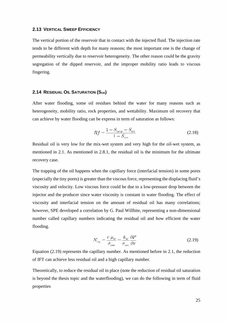
2.14 RESIDUAL OIL SATURATION (SOR)
After water flooding, some oil residues behind the water for many reasons such as
heterogeneity, mobility ratio, rock properties, and wettability. Maximum oil recovery that
can achieve by water flooding can be express in term of saturation as follows:
(2.18)
Residual oil is very low for the mix-wet system and very high for the oil-wet system, as
mentioned in 2.1. As mentioned in 2.8.1, the residual oil is the minimum for the ultimate
recovery case.
The trapping of the oil happens when the capillary force (interfacial tension) in some pores
(especially the tiny pores) is greater than the viscous force, representing the displacing fluid’s
viscosity and velocity. Low viscous force could be due to a low-pressure drop between the
injector and the producer since water viscosity is constant in water flooding. The effect of
viscosity and interfacial tension on the amount of residual oil has many correlations;
however, SPE developed a correlation by G. Paul Willhite, representing a non-dimensional
number called capillary numbers indicating the residual oil and how efficient the water
flooding.
(2.19)
Equation (2.19) represents the capillary number. As mentioned before in 2.1, the reduction
of IFT can achieve less residual oil and a high capillary number.
Theoretically, to reduce the residual oil in place (note the reduction of residual oil saturation
is beyond the thesis topic and the waterflooding), we can do the following in term of fluid
properties

26
1. Reduce the mobility ratio as much as possible by reducing oil viscosity or increasing
water viscosity. That lead to two things:
A. Prevent the fingering of water and the early breakthrough so that Sor will be less.
B. As mentioned before in 2.8.1, achieving the ultimate recovery when the fractional
flow curve will shift to the right and more straighten than S shape leading most
of the saturation having the same velocity and the Swf will be the highest.
2. Reduce the interfacial tension between oil and water by adding a surfactant or
increase the temperature, and that can lead to:
A. Increase the relative permeability for both fluid, oil, and water and by that reduce
the Sor.
B. Increase the capillary number.
3. The imbibition is more efficient than drainage for water flooding means
waterflooding in the water-wet system is more efficient than in the oil-wet system,
as mentioned in 2.1.
The other important parameters that control the residual oil is the rock properties
1. Mixed water-wet can achieve low residual oil in place, as mentioned in section 2.2.
2. As mentioned above, the imbibition is more efficient, so alter the wettability can
change the process from drainage to imbibition. Waterflooding in the oil-wet system
is less efficient because of its drainage process, so if there is any possibility of altering
the wettability to water wet, the process will be imbibition and can be done by
injection low salinity water, for instance.
3. A less heterogeneous and more minor anisotropy system leads to having less residual
oil and place; therefore, recovery factor increases yields zero Dykstra-Parsons’
coefficient.

27
3 CHAPTER THREE: THE DEVELOPMENT HISTORY OF WATER FLOODING
Water flooding has taken the researchers’ paramount importance since years when the oil
industry hit the road to be the first and the most demand energy resource. Since that time,
the companies and the investors have been researching the possibility of increasing oil
recovery factor. Before 1920, researchers and engineers thought that water is detrimental to
the reservoir. Waterflooding accidentally proved an increase in the recovery after the plug
of an old well was destroyed in 1880. The first systematic study performed in 1880 by Carll
illustrates the possibility of increasing oil recovery by injecting water. Initially, there was no
injection wells pattern; the circle method was used, consisting of one injector well in the
field center, till 1925 when Umpleby stated the injection well layout (pattern) and reported
the five-spot pattern (Umpleby, 1925). Barb and Shelley in 1930 show the possibility of
using hot water injection. Due to the long history of water flooding, the important stations
will cove in this literature review as follows:
3.7 ONE-DIMENSIONAL FLOW STUDIES
Buckley and Leverett (1941) introduced a method to normalize the Pc vs. Sw curve from
various core samples, and it is known currently by the Leverett J function (Leverett, 1941).
Buckley and Leverett have proposed the most exciting approach to waterflooding. For some
years, Buckley and Leverett’s theory has received much attention from researchers. The
following context showing the essential stations of Buckley and Leverett equations
development:
Buckley and Leverett (1942) formulated a well-known theory called frontal displacement
theory deriving two equations, Fractional flow and front advance equation, considering that
displacement oil by water is an unsteady-state process. Appendix A describes all the
mathematical derivations of these equations. More theoretical details available in 2.8.
Before 1950, few studies have been published on water flooding. After 1950, many papers
were published, and Various approaches have been proposed, such as the reservoir
simulation idea.
Terwilliger and his co-authors 1951 subdivided Buckley and Leverett saturation distribution
with distance into two zones, stabilize zone from Swf and Swc where all saturations have the

28
same position and velocity. The other zone is the unstabilized zone between Swf and (1-Sor),
where the velocity is different for each saturation (Terwilliger, 1951).
Welge (1952) extended Buckley and Leverett by deriving the slope equation and proposed
graph solution (Welge, 1952). The derivation of the Welge approach is available in Appendix
A.
Levine conducted an experimental study in 1954, observing the effect of viscosity on water-
oil relative permeability. He also investigated the impact of the capillary pressure on Buckley
and Leverett fractional flow when he concluded that neglecting the capillary effect gives a
good result. However, when the capillary effect is defined, the calculated fraction of
displacing fluid increases, and the displaced fluid recovery decreases (Levine, 1954).
J.G Richardson 1957 performed an experimental study that proved that Buckley and
Leverett’s theory is true (Richardson, 1957).
Although this approach of 1D flow is revolutionary, it suffers from addressing the flow when
the displacing fluid is not 100% in contact with the pore volume. For that reason, researchers
tended to focus on the areal sweep efficiency (2D flow).
3.8 AREAL SWEEP EFFICIENCY (2D)
Later, areal sweep, efficiency had the great attention of the reservoir’s engineers. Assuming
that reservoir is horizontal plane, homogenous and uniform thickness, the water is flooding
in two directions x and y. 2D flow observed if permeability varies with position in the
reservoir, the gravity segregation of injected and displaced fluids occurs, and when capillary
forces are large relative to viscous forces (Willhite, 1986). Many correlations were
developed to predict the oil recovery and waterflooding performance by experiments study
models of water flooding. The experiments used different types of models to simulate the
reservoir like sand bed or glass. Furthermore, the studies used various techniques to track
the fluids’ flow, such as fluid mapper, potentiometric models, and X-ray shadowgraph
techniques (Warner, 2015). Table B-1of Appendix B contains all the authors and their
methods.
1. Potentiometric models: the method uses experimental electrolyte setup and uses of
the identically between steady-state Darcy law and Ohm’s law (Morris, 1949).

29
(3.1)
(3.2)
2. Shadowgraph: this method uses X-ray to track the liquid in the porous media stated
in 1951 by Laird and Putnam (Laird, 1951). The X-ray can illustrate the liquid after
either adding potassium iodide to water or adding iodobenzene to oil.
3. Electrical resistivity Models: this method used the resistance network approach,
which results in potentiometric models. Nobles and Janzen first used it in 1958 within
their experimental study (Nobles, 1958).
4. Multipattern scaled experimental setups: this method is found in 1958 by Rapoport
(Rapoport, 1958). Porous media consist of glass beds or powders, and the flow is
affected by capillary pressure and viscus force, but the gravity effect is neglected.
5. Numerical Methods: Many Numerical methods are used to simulate the water
flooding process assuming homogenous porous media. The numerical methods are
the finite difference model and the streamlines model. The first studies of finite-
difference Models considered it to be a valuable approach for water flooding. FD
method approximates the continuous differential equations by finite difference
equations that can be solved by simple algebra.
The other Numerical method is the streamline model that Higgins and Leighton
firstly developed (Higgins, 1961) (Higgins, 1962) (Higgins, 1966). The point of this
method is to divide the reservoir into channels. Currently, many software can analyze
numerical models very quickly by griding the reservoir.
3.8.1 AREAL SWEEP PREDICTION METHODS
Many authors try to find a relationship to predict areal sweep efficiency at and after
breakthrough. Only standard, new, and essential correlations are mentioned as follows:
The correlation that developed by Craig-Geffen-Morse (CGM) on five-spots by using
shadowgraph X-ray. It is a graphical relationship.

30
Willhite developed a correlation to compute EAbt (Willhite, 1986) as in the following
equation.
(3.3)
Dyes and his co-authors developed a graphical correlation between areal sweep efficiency
and the mobility ratio’s reciprocal. He correlated the areal sweep after the breakthrough with
the ratio of the injected volume at any time to the injected volume at the breakthrough (Dyes,
1954). Equation (3.4) and equation (3.4) represents Dyes correlation.
(3.4)
Or
(3.5)
Fassihi used non-linear regression to fit the Dyes curve by using the following regression
(Fassihi, 1986) :
(3.6)
Table B-2 contains a table that shows all coefficients of equation (3.6).
Willhite proposed another correlation to calculate the areal sweep efficiency after the
breakthrough (Willhite, 1986).
(3.7)
Where
(3.8)
(3.9)

31
This correlation has an appendix of tables that areal sweep efficiency can be found
depending on the value of the fraction . Appendix A contains the derivation of
equation (3.7).
Ei(x) function that appears in the solution of the diffusivity equation appears here as well
in equation (3.7). It can approximate by the following:
(3.10)
Willhite also proposed a theory to calculate the water-oil ratio by divide the swept area into
zones, previously swept, which produce water and oil; on the other hand, newly swept where
only oil is produced, and the saturation of this zone is the front saturation. Equation (3.11)
estimate the produced oil for the new swept area.
(3.11)
During a phone interview conducted on March 17, 2021, Mr. Alamara Hatem2 proposed a
simplified correlation to quantify the areal sweep efficiency at the breakthrough as in the
following equation.
(3.12)
All the correlations mentioned above is for an ideal reservoir with many assumptions; the
assumptions are (Ahmed, 2018):
• Isotropic.
• No fracture.
• Confined patterns.
• Uniform saturation.
• Off-pattern wells.
Off-pattern wells mean when the ideal pattern is not complete, or some wells are located in
an unideal place, decreasing the attainable recovery from an ideal pattern (Prats, 1962).
Some correlations tried to ignore one or more of the above assumptions to get a picture of
the performance of the flooding for the non-ideal case,
2 Personal communication

32
Landrum and Crawford conduct a study in 1960 showing the effect of directional
permeability on areal sweep efficiency (Bobby L Landrum, 1959).
3.9 VERTICAL SWEEP EFFICIENCY STUDIES
During geological precipitation, sediments precipitated horizontally, forming different
layers with different properties yield vary of permeability in the vertical direction; the
researcher tried to model the effect of heterogeneity on water flooding as follow:
Craig points out the minimum number of layers required to simulate the actual water
flooding process listed in tables (Craig, 1971).
Miller and Lents proposed geometric average permeability in 1966, assuming injecting fluid
flood in the same height from the injector to producer (Maurice C. Miller, 1966).
Dykstra and Parson did significant work in term of vertical sweep efficiency as follow
1. Quantify the heterogeneity by proposing a coefficient as described in section 2.7.
2. Establish a method for ordering permeability in 1950 by proposing a probability
curve for permeability.
3. Correlate the vertical sweep efficiency with mobility ratio, Dykstra-Parson
coefficient, and WOR (Dykstra, 1951). (See Figure 3-1).
Figure 3-1. Dykstra and Parson correlation
(Dykstra, 1951).

33
4. He proposed a correlation for predicting the recovery by mobility ratio, Dykstra-
Parson coefficient, and WOR.
Johnson proposed a graphical approach for Dykstra and Parson in 1956 for predicting the
overall recovery for different WOR (Johnson, 1956).
Felsenthal, Cobb, and Heuer modified Dykstra and Parson’s works in 1962 to include the
initial gas saturation presence effect at a constant injection rate (Martin Felsenthal, 1962).
Stiles pointed out the water flooding in a layered reservoir, stating that the breakthrough
occurs in sequence, firstly with the layer with the highest permeability, but assumes that the
displacement is piston-like, formulating an equation for calculating vertical sweep efficiency
as in equation (3.14). He has also proposed a formula for calculating the water-oil ratio
(Stiles, 1949).
(3.13)
De Souza and Brigham conducted a regression analysis in 1981, grouping vertical sweep
efficiency for different mobility ratios in one curve (A.O. de Souza, 1995). Equation (3.14)
and equation (3.15) the formula of linear regression used by the authors.
(3.14)
(3.15)
Figure 3-2. EV versus the correlating parameter Y
(A.O. de Souza, 1995).

34
Fassihi used a non-linear function to fit the graph of De Souza and Brigham results in 1986
(See Figure 3-2) as in the following equation:
(3.16)
Where
a1=3.334088568
a2=0.7737348199
a3=1.225859406
Equation (3.16) is Fassihi’s non-linear function that can be solved by numerical methods
like Newton -Raphson methods (Fassihi, 1986). To avoid the iterative process, Ahmed
proposed using the Taylor series (Ahmed, 2018).
Craig and his co-author suggest doing the calculation layer by layer in stratified reservoirs
(Craig, 1955).
Alhuthali et al. (2006) conducted a robust optimization to maximize the reservoir’s sweep
efficiency, and they used different geological scenarios based on adjusting the waterfront’s
breakthrough time for all producers to achieve the breakthrough at the same time.
Meshioye et al. 2010 proposed a method in which waterflooding has been controlled by new
injector well technology to maximize the project's net present value.
Ogali (2011) implemented research to optimize waterflooding by streamline simulation.
3.10 WATERFLOODING SURVEILLANCE
3.10.1 HALL PLOT
Hall proposed a steady-state method to analyze the injector’s performance by plotting the
integral term of pressure-time curve vs. cumulative injected water (Hall, 1963). The Hall
plot slope gives a qualitative measurement for the transmissibility of the well to the injected
fluid. It is a widespread method because it required simple surface data like the wellhead
pressure after converting it to bottom hole flowing pressure by the pressure traverse
calculations and its required injection rate (P.M. Jarrell, 1991).

35
(3.17)
(3.18)
Equation (3.18) represents the slope of the Hall plot that supposed to be constant for stable
waterflooding, but it might change because the skin changes; for instance, if the pressure
exceeded the fracture pressure, the formation would get fractured, and the skin will be
negative; therefore, the slope of the curve will decrease. The injection radius increases
continuously with the increase of the injected water, as in equation (3.19). The change of
radius has a slight effect on Hall’s plot because it is within the logarithmic term as in equation
(3.18). However, the impact of the radius increment is pronounced in the early time, and it
is called the fill-up period. (See Figure 3-3).
𝑟𝑒 = √5.615 𝑊𝑖
𝜋 ℎ ∅ [̅̅̅̅ − 𝑆𝑤𝑖] (3.19)
Figure 3-3. Typical Hall plot for various conditions
(SPE).
Izgec and Kabir 2007 (Bulent Izgec, 2007) proposed another diagnosis check extending Hall
plot by drawing the derivative of Hall plot curve with Hall function, and the result curves
will follow three cases as follow:

36
• Both plot DHI and HI on the same straight line means there is no change in the
wellbore skin.
• DHI falls below the HI curve, which means the formation has fractured, therefore
yield negative skin factor.
• DHI falls above the HI curve, which means the formation has a positive skin factor.
Many researchers extend Hall plots like Ojukwu and Van den Hoek 2004 (Ojukwu, 2004),
Siline and his co-authors 2005 (Dmitry B. Silin, 2005), and b (Dmitry B. Silin, 2005-03-30).
3.10.2 HEARN PLOT
Hearn proposed a steady-state radial Darcy law method to quantify the water-relative
permeability and diagnose the injector’s wellbore damage. Its modification of the Muskat
method for constant pressure (Hearn, 1983). Both Hearn and Hall blot uses radial steady-
state Darcy law, but the difference the first develop a straight line during the fill-up period
while the second develops a straight line after the fill-up part. Hearn plot is a simple
surveillance method that’s required simple data in hand, which is wellhead pressure,
reservoir pressure, and the injection rate by drawing the injectivity index vs. cumulative
injected water as shown in Figure 3-3. Hall and Hearn’s application is to reduce the cost of
performing periodic step-rate tests to measure fracture pressure. Hall and Hearn’s plot
indicates if we have exceeded the fracture pressure or not, and by that, we can increase the
injection rate as much as possible. The increasing injection rate can calibrate the following:
• Prevent tonging due to gravity segregation by keeping the injection rate above the
critical rate as mentioned in section 2.4.
• Increase the viscous force and increase the capillary number to achieve the ultimate
recovery, as mentioned in section 2.14.
• Increase reservoir pressure build-up.

37
Figure 3-4. Hearn plot illustrating interpretations of various slope changes
(Warner, 2015).
3.10.3 DECLINE CURVE (DC)
The decline curve analysis golden rule is that the future performance can follow the past
production behavior, so any formula or equation that simulates the production history can
predict the production. DC is the most common technique in the mature oil field where
sufficient production data are available (Ronald Harrell, 2004). It more like a statistical
method depend on the data in hand (Production history) and how production behaves. Arps
stated that the character of producing wells seems to regain, more or less, its” individuality,”
and the old and familiar decline curve appears to have had a comeback as a valuable tool in
the hands of the petroleum engineer (ARPs, 1945). Engineers used to linearize the equations
to interpolate and extrapolate the given function’s behavior. This linear decline curve
function achieves by changing the graph type from cartesian to semi-log to log-log scales.
Arps found out that all production wells follow three decline curves, Hyperbolic Model,
Exponential Model, and Harmonic Model (ARPs, 1945). For exponential DC, linear function
founds by graphing flowrate vs. time on a semi-log scale or flowrate vs. the cumulative
production on a cartesian scale.
For hyperbolic DC, no linear function can be found if the graph type changed, but if we draw
flow rate vs. time in log-log scale and with some shifting technique, a linear function can be

38
result. A linear function is found by graphing flow rate with the cumulative production on a
log-log scale for harmonic DC, as shown in the following figure:
Figure 3-5. Classification of production decline curves
(Arps, 1956).
The decline rate (D) is how much the production loss per unit of time, which is the first
derivative of the flow rate vs. time of a semi-log curve; its function of time and hyperbolic
exponent. Hyperbolic exponent is the change of decline rate with time, and it also can be
identified as the second derivative of the flow rate vs. time of the semi-log curve as in
equation (3.21). The exponential decline has a constant decline rate in flowrate vs. time semi-
log curve; therefore, the hyperbolic exponent (b), or the curvature, or the second derivative
of the exponential decline model is zero. The hyperbolic decline has a variable decline rate
and changes with time but with a constant rate; by that, the second derivative of the semi-
log flow rate vs. time curve is constant. The more hyperbolic exponent we have, the faster
transition from high to lower decline curve where the harmonic decline occurs (Purvis,
2016). Mathematically decline rate is the ratio between the natural logarithm of the flow rate
to the time as in equation (3.20).
𝐷 = −
𝑑(ln 𝑞)
𝑑𝑡= −
1
𝑞 𝑑𝑞
𝑑𝑡 (3.20)

39
𝑏 =
𝑑
𝑑𝑡 (
1
𝐷) (3.21)
The exponential and harmonic models are specific cases of the hyperbolic model with
constant decline exponent (b) of 0 and 1, respectively (SPE, AAPG, WPC, SPEE, SEG,
2011).
The table below listed the equation that can be used for the DCA (SPE, AAPG, WPC, SPEE,
SEG, 2011).
Table 3-1.
Traditional decline analysis: governing equations and characteristic linear Plots.
Generalized governing hyperbolic decline equation:
Hyperbolic Model Exponential
Model
Harmonic Model
Nominal Decline Rate
(D)
Dt =Di = Dt=constant
Decline Exponent (b) “b” varies approximately
constant
except for 0 & 1
b=0 b=1
Rate -Time
Relationships
Type of Linear Plots: log Qt vs. log (1+C t)
where C=bDi
log Qt vs. t Qt vs. Npt
1/Qt vs. t or
log Qt vs. log (1+Di
t) log Qt vs. Npt
i = stands for initial time or point at which the decline trend has onset or started.
Dt = nominal decline rate (as a fraction of Qt) with a unit of inverse time (1/t), equals to Di when
Qt= Qi.
Qt = oil or gas production rate at any time “t” in STB/D or MMscf/D, etc.*.
t = time and the subscript for oil rate & cumulative production variables*.
Npt = cumulative oil or gas production or oil recovery at any time “t” inconsistent units*.
* Rate (Q) & time (t) must be inconsistent units in above formulae (i.e., if “Q” is in STB/D, “t”
is in days, etc.).
Source: (SPE, AAPG, WPC, SPEE, SEG, 2011)

40
4 CHAPTER FOUR: SIMULATION AND PRODUCTION DATA
ANALYSIS
The study field is undersaturated carbonate oil reservoir was put into production at the end
of 1976, and the production reached the peak of 41 MSTB/day in May of 1980. The
development history of the field is divided into five periods: the initial production period
from 1976 to 1980, the shut-down period from 1980 to1998, the re-open production period
from1998 to 2010, the depletion period from 2010 to 2016, and the water flooding period
after 2016. The reservoir formation is divided into three zones comprising nine layers. The
primary layer is MB21 and characterized by distributional stability, with a flattening
thickness of 83.2m. Only reservoirs of MB21, MC11, and MC2 developed well in the whole
area with an average reservoir thickness of 83.2m, 15.7m, and 34.1m, respectively (See
Figure 4-2). The average reservoir thickness of other zones ranges from 0.1 to 9.5m, as
shown in Figure 4-1.
Figure 4-1. Reservoir layer distribution.

41
Figure 4-2. Reservoir thickness of zone/sub-zone.
The NTG (net to gross) is pretty different between the different zones, ranges from
0.4%~98.2%, the maximum is almost 100% in MB21, and MC2 is the second highest, which
is much higher than the other zones as shown in Figure 4-3.
Figure 4-3. NTG of zones/sub-zones.
The net pay thickness differences between different sub-zone/zone are significant. The
thickness of MB21 is the greatest, of which the average thickness is 72.0m. All the other
zones or sub-zones net pay thicknesses are nearly below 10.0m, ranging from 0.0m~9.0m
(See Figure 4-4).

42
Figure 4-4. Net oil thickness of zones/sub-zones.
The initial reservoir pressure is 6300 psi; unfortunately, it depleted severely, reaching the
reservoir’s static pressure is 4200 psi. The bubble point pressure is 2660 psi, while currently,
the difference between reservoir pressure and bubble point pressure is about 1540 psi. Crude
oil viscosity is 0.83-1.83mPa·s under formation pressure. The dissolved gas-oil ratio is 692
SCF/STB, crude oil formation volume factor under formation pressure is 1.4146 bbl./STB,
and crude oil formation volume factor at bubble point pressure is 1.429 bbl./STB. It was
decided to inject water in the MB21 layer because it is the main pay zone, the large thickness,
the highest amount of original oil in place, and the zone is under production by most of the
producer wells. Based on the well logging interpretation data, it decided that for
waterflooding, MB21 needs to be subdivided into six sublayers (Drains) D1, D1D, D2, D2D,
D3, D3D. The permeability of the D1, D2, and D3 MB21 layer are 16.7mD, 22.3 mD, and
15.5 mD, respectively, showing relatively high permeability. On the contrary, the
permeability of D1D, D2D, and D3D of MB21 layer are 4.3mD, 3.9 mD, and 3.1mD,
respectively, indicating relatively low permeability (see Figure 4-5). It was decided to inject
through D3D and D3.

43
Figure 4-5. MB21 sublayers.
Repeat formation tester (RFT) confirmed good vertical conductivity of MB21 because the
pressure drops due to the primary recovery period occurred along with all the thickness of
MB21. The modular formation tester confirmed this conductivity as the same slop along
the pressure gradient, as shown in Figure 4-6. It was found that the best strategy is
produced from top and inject from bottom (PTIB), which conformed by RFT, MDT, and
simulation.
Figure 4-6. Pressure gradient for several wells in the field.

44
4.1 THE STUDY SECTOR OF NINE-SPOT PATTERN.
The thesis scope of work is to study water flooding in a part of the reservoir (Sector model).
It was decided that the best procedure for studying waterflooding is to choose a part of the
field to have a representative sector model to evaluate the current waterflooding within a
specific pattern. The invert nine spot patterns have been selected in this study because it is a
complete pattern and a good candidate for study purpose since the injector well (Well-36)
start injection on 27 Oct 2017. It is worth to be mentioned that Well-36 was producer well
since 2013 with average oil production of 1800 STB/day; Figure D-20 and Figure D-19 in
Appendix C show the production performance for Well-36. The wells and the start
production time are listed in Table 4-1. Well-7 has stopped production since 1980. Appendix
B contains the production performance of all the wells within the pattern. Figure 4-7
illustrates the invert nine-spot pattern and the well location within the pattern.
Figure 4-7. Invert nine-spot pattern of Well-36 (The study Sector).

45
Table 4-1.
The wells of the study sector.
No. Well Time of production Well type Unit Status
1 Well-36 27-Oct-2017 Vertical, Injector MB21 Active
2 Well-16 13-Nov-1998 Vertical,
Producer MB21 Active
3 Well-47 17-Jun-2016 Vertical,
Producer MB21 Active
4 Well-116 29-Mar-2020 Vertical,
Producer MB21 Active
5 Well-50 25-Dec-2015 Vertical,
Producer MB21 Active
6 Well-6 2-Apr-1977 Vertical,
Producer MB21 Active
7 Well-53 16-Aug-2015 Vertical,
Producer MB21 Active
8 Well-15 25-Dec-2002 Vertical,
Producer MB21 Active
9 Well-69H 24-Feb-2018 Horizontal,
Producer MB21 Active
10 Well-7 27-Mar-1977 Vertical,
Producer MB21 Shut-in

46
4.2 PRIMARY AND SECONDARY FORMATION PRESSURE MAINTENANCE
ANALYSIS.
The initial formation pressure of the oilfield is 6300 psi. Due to a shortage of natural energy,
the average formation pressure decreased fast. Currently, the average formation pressure is
4200 psi, which is low because of the inactive aquifer (See Figure 4-8). Figure 4-9 illustrates
the study sector pressure performance with time, which follows the field’s depletion
performance.
Figure 4-8. Pressure variation diagram of the whole reservoir.
Figure 4-9. Pressure variation diagram of the Sector (the invert nine-spot pattern).
0.00
1000.00
2000.00
3000.00
4000.00
5000.00
6000.00
7000.00
Jan-76 Sep-89 May-03 Jan-17
Stat
ic P
ress
ure
Date
Pb=2660 psi

47
According to a drive mechanism diagnosis, it is evident that the reservoir is an undersaturated
depletion reservoir. Dake, Campbell, and a new approach were chosen to diagnose the drive
mechanism. These methods use the material balance equation principle to identify the
predominant drive mechanism.
Dake and Campbell proposed a diagnostic method to diagnose the reservoir’s drive
mechanism depending on the graph of F/Et Vs. Np or F (Dake, 1994) (Campbell, 1980).
Figure 4-10. A. Dake Plot. B. Campbell plot
(Alamara, 2020).
The result for Dake and Campbell plots of the study sector has shown volumetric depletion
before the water flooding, but it is obvious the effect of water flooding in the last points,
indicating another mechanism start to act (See Figure 4-11). The calculation table for
Figure 4-11 is available in Table B-4 within Appendix B.
B A

48
Figure 4-11. Diagnostic plot for the sector
A. Dake Plot. B. Campbell plots.
Li and Zhu (Li CL, 2014) proposed a new diagnostic method depend on the material balance
equation by drawing Dpr vs. Npr at which Dpr is the formation pressure decline
corresponding to 1% OOIP recovery,” and Npr is the elastic production ratio as the following
equations:
𝑁𝑝𝑟 =
𝑁𝑝 𝐵𝑜
𝑁𝑝 𝐵𝑜𝑖 𝐶𝑡 (𝑃𝑖 − �̅�) (4.1)
𝐷𝑝𝑟 =
𝑁 (𝑃𝑖 − �̅�)
100 𝑁𝑝 (4.2)
Reservoir natural energy is classified into four categories, as in Figure 4-12, and BU-S refers
to the whole reservoir of the study field located in the weak natural energy region.
0
200
400
600
800
1000
0 5 10 15 20 25 30 35
F/Et
Np
Before waterflooding
0
200
400
600
800
1000
0 10 20 30 40 50
F/Et
F
Before waterflooding
A
B

49
Figure 4-12. Natural energy classification evaluation chart of the whole reservoir.
The chart of the study sector shows a unique behaver because it included the data after
waterflooding. In the natural flow period, the point was located in the weak natural energy
area. The point starts to move to the right where Npr is increasing, revealing the
waterflooding effect and that have a good agreement with Dake and Campbell plots. The
data of Figure 4-13 available in Table B-4 within Appendix B.
Figure 4-13. Natural energy classification evaluation chart of the sector.
0.01
0.1
1
10
0.1 1 10
Dp
r
Npr

50
4.3 PRIMARY AND SECONDARY MATERIAL BALANCE CALCULATIONS.
Schilthuis is the first who developed the general material balance equation in 1935
(Schilthuis, 1936); since that time, MBE became an essential tool in reservoir engineers’
hands. It implies the well-known golden rule that states production equals expansion plus
water influx and water injection, known as “conservation of matter.” For simplicity, the
assumption is that the sum of all volume changes is equal to zero. The method assumes that
the reservoir is considered a tank, uniform average reservoir pressure, no change in
hydrocarbon composition, only three fluid, and no chemical reaction. Furthermore, the
reliability of the method depends mainly on the pressure, production, and PVT data.
The uses of material balance (Alamara, 2020)
• Estimation tool: Determining the initial hydrocarbon in place, water influx, and
initial water in place.
• Prediction tool: To predict the reservoir performance such as recovery factor, water
influx, oil saturation, and production.
• Dignostive tool: to understand the reservoir mechanism as explained in section 4.2.
• Characterstive tool is to calculate the permeability when combined with Darcy
equation resulting in diffusivity equation used in pressure transient analysis to
quantify permeability.
• Inspective tool: to history matching the data.
MBE was used to determine one parameter only, for instance, original oil in place until
Havlena and Odeh proposed a brilliant work in 1963 to linearize the material balance
equation. Hence, it becomes possible to determine more than one parameter using the
straight-line features as the slope and the intercept (Havlena, 1963), adding a dynamicity to
the MBE, raising it from a single point solution to a multipoint straight line (Alamara, 2020).
Since the reservoir is undersaturated, as explained in section 4.2, and the aquifer is fragile,
the pot aquifer model is used, and Havlena and Odeh have applied to the sector (the invert
nine-spot pattern). The following equations describe all the terms for the MBE used in the
study sector calculations.
𝐹 = 𝑁 (𝐸𝑜 + 𝐸𝑓𝑤) + 𝑊𝑒 + 𝑊𝑖 𝐵𝑤 (4.3)
Where

51
𝐹 = 𝑁𝑝 [𝐵𝑜 + (𝑅𝑝 − 𝑅𝑠𝑖) 𝐵𝑔] + 𝑊𝑝 𝐵𝑤 (4.4)
And
𝐸𝑜 = (𝐵𝑜 − 𝐵𝑜𝑖) (4.5)
𝐸𝑓𝑤 =
𝐵𝑜𝑖
(1 − 𝑆𝑤𝑖) (𝑆𝑤𝑖 𝑐𝑤 + 𝑐𝑝) (4.6)
Equation (4.7). is the MBE material balance equation.
𝐹 − 𝑊𝑖𝑛𝑗 𝐵𝑤
(𝐸𝑜 + 𝐸𝑓𝑤)= 𝑁 + 𝐵
∆𝑝
(𝐸𝑜 + 𝐸𝑓𝑤) (4.7)
Where
𝐵 = 𝑊𝑖 𝐶𝑡𝑒 (4.8)
The straight-line model results show that the original oil in place is equal to 250 MM, and
the pot aquifer constant is 0.00091, which represents the total compressibility of the aquifer
multiply by the water initial in place of the aquifer. The Havlena and Odeh model results are
shown in Figure 4-14, and the calculation result is listed in Table B-4 in Appendix B.
Figure 4-14. Havlena and Odeh model for the sector.
The use of the unique feature of material balance by converts the equation into drive indices
to describe each drive's contribution. Drive indices can be done by dividing both sides by
the total hydrocarbon production as the followed equations:
y = 0.0156x + 250.67
0
500
1000
1500
2000
2500
0.27 0.27 0.27 0.27 0.27 0.27
(f-W
i)/E
t
Dp/Et
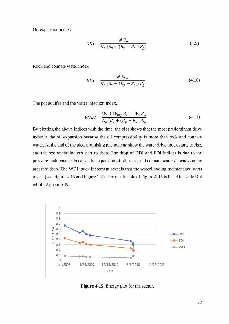
52
Oil expansion index.
𝐷𝐷𝐼 =
𝑁 𝐸𝑜
𝑁𝑝 [𝐵𝑜 + (𝑅𝑝 − 𝑅𝑠𝑖) 𝐵𝑔] (4.9)
Rock and connate water index.
𝐸𝐷𝐼 =
𝑁 𝐸𝑓𝑤
𝑁𝑝 [𝐵𝑜 + (𝑅𝑝 − 𝑅𝑠𝑖) 𝐵𝑔 (4.10)
The pot aquifer and the water injection index.
𝑊𝐼𝐷𝐼 =
𝑊𝑒 + 𝑊𝑖𝑛𝑗 𝐵𝑤 − 𝑊𝑝 𝐵𝑤
𝑁𝑝 [𝐵𝑜 + (𝑅𝑝 − 𝑅𝑠𝑖) 𝐵𝑔 (4.11)
By plotting the above indices with the time, the plot shows that the most predominant drive
index is the oil expansion because the oil compressibility is more than rock and connate
water. At the end of the plot, promising phenomena show the water drive index starts to rise,
and the rest of the indices start to drop. The drop of DDI and EDI indices is due to the
pressure maintenance because the expansion of oil, rock, and connate water depends on the
pressure drop. The WDI index increment reveals that the waterflooding maintenance starts
to act. (see Figure 4-15 and Figure 1-2). The result table of Figure 4-15 is listed in Table B-4
within Appendix B.
Figure 4-15. Energy plot for the sector.
0
0.1
0.2
0.3
0.4
0.5
0.6
0.7
0.8
0.9
1
1/1/2002 6/24/2007 12/14/2012 6/6/2018 11/27/2023
DD
I,ED
I,W
DI
date
DDI
EDI
WDI

53
4.4 PRIMARY AND SECONDARY PRODUCTION DATA ANALYSIS.
The study sector (the invert nine-spot pattern) oil rate, water rate, cumulative oil rate for 45
years from 1976 through 2021 are shown in Figure 4-17 and Figure 4-18. All the production
history could be classified under natural primary recovery until Oct 2017, when a
waterflooding secondary recovery has been imposed to maintain the pressure and increase
oil recovery. The field was shut-in during the period from 1976 to 1998, and Figure 4-17
shows a different trend of the cumulative oil, and the most interesting is the last trend shows
a change in the slop after 2017, which indicates the effect of the waterflooding. The
maximum oil rate for the sector was 8000 STB/day with free water before the waterflooding,
while it reached 15000 STB/day and 17.5% water cut after the water flooding with 8000
bbl/day of injection rate. Oil rate fell since 1976 then began increasing after 2017 as water
injection started, as shown in Figure 4-16. Decline curve analysis revealed that from 2012 to
2016, the natural decline rate was 16.4% for the sector, as shown in Figure 4-19. Annually
decline curve calculations from 2012 to 2015 for the sector available in Appendix C.
Figure 4-16. The sector production rate Performance.
Figure 4-17 illustrates the cumulative oil and production rate for oil and water, which reveals
the change of the cumulative slop due to the change of the production rule, especially the
last slop change after 2017 where the water injection was imposed to the sector.

54
Figure 4-17. Cumulative production, oil rate, and water rate for the sector.
The following Figure 4-18 delineates the cumulative stack contribution of oil and water
bring to light that only minor water has been produced since 1976 assure the weakness of
the aquifer.
Figure 4-18. Stacked cumulative oil and water production for the sector.

55
The following Figure 4-19 represents the annual decline curve to illuminate the severe
decline has occurred before 2015 through the weak depletion drive mechanism for the
undersaturated reservoirs.
Figure 4-19. The natural decline curve of oil wells of the sector.
Some wells within the pattern have not been drilled till 2020, when well-116 has drilled.
Figure 4-20 illustrates the flow rate for the ten wells within the pattern. In the beginning,
only well-6 and well-15 were producing with a high production rate of approximately 2500
STB/day; therefore, these two wells achieved the highest cumulative oil rate, as shown in
Figure 4-21.
2012
DC= 8.3%
2013
DC= 12.9%
2015
DC= 16.4%
2014
DC= 14%

56
Figure 4-20. A plot of the daily oil rate for each well within the sector.
Figure 4-21. Sector wells cumulative oil rate.
After waterflooding, the DC result shows an incline in the trend where the decline rate is
negative, which confirms the water flooding effect shown in Figure 4-22. last period of
production, the DC start to decrease because the operator has to chock on the production for
some policy. The dashed line in Figure 4-22 simulates the decline curve if the production
continues without the policy because the decline curve after 2019 simulates by a blue arrow
to the right of Figure 4-22 reveals the same DC value of -10%.

57
Figure 4-22. Decline curve result for the sector after the waterflooding.
The bubble map prior and post water injection revealed some water start grown in the last
years, as shown in Figure 4-23 and Figure 4-24.
Figure 4-23. Sector bubble map of 2021.
2018
DC= -10%
From 2018 to present time, production policy.
DC= -10%

58
Figure 4-24. Sector bubble map before water injection in Oct 2017.
Bubble maps show that a might breakthrough starts to develop mainly in well 6, 16, and 47.
Voidage replacement calculations unveil that there might be a water breakthrough when
cumulative oil starts to deviate from cumulative liquid imply that water production starts
growing, but this growth is not water breakthrough because this water produces from Well-
69. Well-69 starts producing water immediately when putting it in production after
waterflooding, leaving the question, how come the water reached the area of no pressure
disturbance streamline where well 7 (shut-in) and well-69 has not drilled yet, as shown in
Figure D-1 within Appendix C more detailed information about the water production of
Well-69 is explained in section 4.6.1. The voidage replacement ratio (VRP) curve shows that
the cumulative VRP was almost 0.6 for the study sector as illustrated in Figure 4-25;
However, the VRP value is 1 for the whole oil field, and this is the planned value to develop
the field.

59
Figure 4-25. Instantaneous and cumulative voidage replacement and cumulative liquid and
oil for the sector.
4.5 INJECTOR DATA ANALYSIS
Well-36 has converted to injector at the end of Oct. 2017. The injection rate is about 8000
bbl/day. Figure 4-26 shows the injection performance where wellhead pressure increased at
the end of 2018. Hall and Hearn's plots described in sections 3.10.1 and 3.10.2 revealed a
fill-up period of low wellhead pressure (Transient period) as shown in Figure 4-27 and
Figure 4-28, where the change in the slop of Hall plot indicates the resistance of the reservoir
pressure when the water reached the boundary; therefore, the pressure maintenance supposes
to start after fill-up period. The injectivity index calculates by the reciprocal slope of the Hall
plot after the fill-up period, and it is about 1.35 bbl/psi, as shown in Figure 4-29. Figure D-21
in Appendix C illustrates the completion design of well-36 where injection only in D3 and
D3D to inject from the bottom and produce from the top (D1, D1D, D2, D2D).
0
0.2
0.4
0.6
0.8
1
1.2
0
2
4
6
8
10
12
14
16
6/14/2017 4/10/2018 2/4/2019 12/1/2019 9/26/2020 7/23/2021
VR
P
Np
+Wp
Mill
ion
s
DateNp+Wp Np Cum VRP Instant VPR

60
Figure 4-26. Injection performance of Well-36.
The following figure (Figure 4-27) illustrates the Hall plot index and the wellhead pressure
with the cumulative injected water, showing the fill-up period at the beginning where the
low wellhead pressure and low slope occurs then the water wave reached the boundary where
the resistance of the reservoir pressure when more wellhead pressure needed to inject less
water than in fill-up period.
Figure 4-27. Hall plot and bottom hole pressure.
0
1000
2000
3000
4000
5000
6000
7000
8000
9000
10000
0
500000
1000000
1500000
2000000
2500000
3000000
3500000
4000000
0 2 4 6 8 10
Bo
tto
m h
ole
pre
ssu
rep
si
Sum
dp
dt
psi
day
Cumlative water injection MMbblHI Bottom hole pressure

61
Figure 4-28 depicts Hall and Hearn plots were drawn together, which emphasized the fill-up
period where the slop of HI and Hearn's behavior has changed together after the water fill-
up period, the wellbore area, and the invasion radius increase.
Figure 4-28. Hearn and Hall plots.
Injectivity index has been calculated for the post-fill-up period for hall plot, 1.3 STB/d/psi
value obtained for the slope of Figure 4-29 where linear curve-fitting trendline has used.
Figure 4-29. Hall plot straight line post-fill-up.
0
500000
1000000
1500000
2000000
2500000
3000000
3500000
4000000
0
0.2
0.4
0.6
0.8
1
1.2
1.4
1.6
1.8
2
0 2000000 4000000 6000000 8000000
Sum
dp
dt
psi
day
1/I
Ip
si/b
bl
Cumulative water injection bblHearn function HI
Fill-up period
y = 0.7383x - 3E+06
0
500000
1000000
1500000
2000000
2500000
3000000
3500000
0 2000000 4000000 6000000 8000000 10000000
Sum
dp
dt
psi
day
Cumulative water injection bblHI Linear (HI)

62
4.6 SIMULATION SECTOR MODELLING
Schlumberger simulators software (Eclipse and Petrel) was used to simulate the pattern by
sector model feature. The simulation sector model is simply simulating part of the reservoir
considering the boundary condition to expedite the simulation run significantly, allowing the
monitoring and calibration of the pattern water injection process. Moreover, achieve the
optimum combination of injection and production rate, much faster simulation run than the
full field model, get fast and reliable data about infill wells possibility, drill a new well, water
breakthrough, fingering, water coning, etc. There are three boundary conditions available for
the sector mode: Flux boundary, Pressure boundary, and no flux boundary (it should not be
classified as boundary even). Flux boundary is captured the fluid flow across the boundary
for each time step applying the material balance equation where the production from the
sector region is limited by fluid initially in the region and the flow into the region. The
Pressure boundary represents the saturation, and pressure around the sector region is
captured for each time step, allowing more fluid to be produced, even more than the initial
oil in the region. No flux boundary is considered the sector as an individual reservoir with
no pressure support and no fluid movement across the boundary. The two boundaries (flux
and pressure boundaries) were used in this study; pressure boundary gave unrealistic
production while flux boundary conditions gave a realistic result. Through the capture of
flux boundary conditions during the run of the full field model, it was able to conduct a
representative simulation sector model for the study. The boundary condition is captured by
run the simulation of the full field model with the history strategy and the planned full-field
prediction strategy.
The sector simulation run model has been done within the capture boundary period only.
The statice properties for the full field model have been used to obtain the dynamic result
for the sector model; the sector model does not require redistributing the properties for the
area of interest. Figure 4-30 shows the 3D model for the full field that illustrates the vertical
and horizontal permeability. Figure 4-31 depicts the porosity distribution for the full field
model. Figure 4-32 is the 3D full-field model for the initial water saturation in 1977.

63
Figure 4-30. A. Vertical permeability B. Horizontal permeability distribution for the field
model.
Figure 4-31. Porosity distribution for the field model.
A
B

64
Figure 4-32. Initial water saturation distribution for the field model.
The following figure (Figure 4-33) shows the sector model where the region has been
selected by using polygon and two surfaces. The wells are shown in the bottom figure as a
top view. Ap1 and Ap2 are wells that the study suggested as appraisal wells shown in the
figure. More details about these appraisal wells in section 4.6.2.
Figure 4-33. The sector model chosen region and the wells.

65
The sector model has been conducted using two strategies; the history strategy from March
1977 to Dec 2018 is the same as the full field model to eliminate the need for history
matching because the full field model is already calibrated. The prediction strategy has been
chosen to optimize the water flooding. The detailed development strategies for the sector
model and the result are as follows:
4.6.1 HISTORY STRATEGY:
The calibrated full-field model strategy is used. Figure 4-34 shows the change of oil
saturation from the start of production till Dec 2018.
Figure 4-34. A. Initial oil saturation B. Oil saturation at the end of 2018.
Figure 4-35 illustrates the bubble map at the end of 2018, which shows that most of the wells
are free of water except Well-69H. To confirm the source of water for Well-69H, the full-
field model shows that the well is near the oil-water contact, and there is an excellent
horizontal and vertical permeability toward the horizontal trajectory of the well, as shown in
Figure 4-36.
A B

66
Figure 4-35. Oil saturation and bubble map for the sector.
Figure 4-36. Well-69H location for A. Full-field water saturation distribution B. Full-field
permeability distribution.
The following figure (Figure 4-37) delineates the water movement around the injector in the
cross-sectional slice before and after the water injection.
A
B

67
Figure 4-37. Cross-section slice for the injector (Well-36) of A. Oil saturation before the
water flooding. B. Oil saturation after the water flooding till the end of 2018.
4.6.2 PREDICTION STRATEGY
Prediction strategy has been chosen to maximize the sector production considering some
restrictions to get a realistic prediction. The production target has been set for the sector as
a group oil rate of 20000 STB/d with a bottom hole flowing pressure limit of 3000 psi to
maintain the pressure above the bubble point pressure (2660 psi). The wells' production
follows the group rate target, the bottom hole pressure limit, and 80 % water cut limit with
the choice of water cut action to shut in the worst connection. Wells water injection rate has
been applied with a bottom hole pressure limit of 9800 psi to keep the injection pressure
below the fracture pressure (11817 psi). Well-47 is planned to convert to injector in 2022,
so the prediction strategy converts this well to an injector at the beginning of 2022 for the
same well control rate and fracture pressure limit. Figure 4-38 depicts the oil saturation in
2040. Figure 4-39 show the water movement around the injector in the cross-sectional slice
after the prediction in 2040 revealed the downward movement of the water, which confirmed
the water injection plan that stated injection in the bottom and produces from the top (PTIB)
to delay the water breakthrough, reduce the residual oil saturation and provide the required
pressure maintenance.
A B

68
Figure 4-38. Predicted oil saturation in 2040.
Figure 4-39. Cross-section slice for the injector (Well-36) of predicted oil saturation after
the water flooding in 2040.
Figure 4-40 plot describes the oil rate, water rate, and water cut rate with time. The simulator
has maintained the oil rate target till 2023; then, the oil production rate starts to decrease
because some wells have reached the limit of either bottom hole or water cut. Appendix E
contains all the well prediction performance of the simulation result.

69
Figure 4-40. The plot of sector oil rate, injection rate, and water cut with time.
Figure 4-41 is a plot of remaining oil and reservoir pressure with time, detect the behavior
change of reaming oil in place after 2017 when the water injection started showing that the
recovery is significantly increased. On the other hand, the reservoir pressure curve has good
agreement with the oil in place curve after 2017, confirming the pressure maintenance and
the recovery efficiency of the water flooding process.
Figure 4-41. Sector remaining oil and reservoir.
Waterflooding
Natural Drive

70
The following figure (Figure 4-42) shows the cumulative liquid and oil, indicate the water
breakthrough in 2022, where cumulative oil starts to deviate from the cumulative liquid. The
current produced water of the pattern comes from Well-69H due to the well location near
OWC, as mentioned in section 4.6.1. After 2022 the water cut starts to develop, as shown in
Figure 4-40, and the simulator has to shut off some wells due to the water cut increment of
more than 80%. Figure 4-43 depicts the predicted oil saturation and bubble map for the
pattern in 2038, where a severe water cut problem occurred within the sector area.
Figure 4-42. Prediction cumulative oil and liquid for the sector model.
Figure 4-43. Predicted bubble map for the sector model in 2040.
Water breakthrough

71
Two appraisal wells have drilled in the simulation where a relatively high oil saturation to
monitor the water injection performance considering the well spacing of 500 m. Table 4-2
listed the suggested wells' location, true vertical depth, measured depth, and the drilling time.
Table 4-2.
Appraisal Wells.
Well
name
X Y TVD MD Time of
drilling
Ap1 2390769.79 11656584.48 12631.9 13883.2 2022
Ap2 2392546.16 11657580.42 12465.6 12465.6 2022
Figure 4-44. Ap1 simulation production performance.

72
Figure 4-45. Ap2 simulation Production Performance.
The following figures (Figure 4-46 and Figure 4-47) illustrate the simulation result of Well-
47 before and after converting it to an injector.
Figure 4-46. Well-47 simulation injection performance.

73
Figure 4-47. Well-47 Simulation Production Performance.

74
5 CHAPTER FIVE: CONCLUSION AND RECOMMENDATIONS
5.7 CONCLUSION AND RECOMMENDATION.
Currently, the formation pressure of the field has dropped severely from 6300 psi to 4200
psi with a 2100 psi pressure drop; consequently, it was necessary to conduct water injection
to supplement energy, extend the natural flow period and maintain high productivity. The
current pressure difference between the average reservoir pressure and the bubble point is
about 1540 psi since the bubble point pressure is about 2660; therefore, the danger of having
free gas in the reservoir is near. Single well productivity is declined, as illustrated in the
decline curve analysis result in Appendix C. Recovery percentage was relatively low and
significant pressure drop before the water injection as the simulation result shown in Figure
4-17. The recovery percentage was 4% for the sector area and 5% for the whole field before
water injection with a formation drop of 2100 psi. The natural energy evaluation result
indicated that natural energy was insufficient, and the simulation result showed no water
drive mechanism, as mentioned in section 4.2. Original oil in place is about 250 MMSTB
for the sector area (Study pattern area) and 4664.99 MMSTB for the whole oil field. MB21
layer is very thick, good continuity, good rock properties indicating that water injection was
feasible.
The current situation of the study sector water flooding has been improved the pressure
maintenance and increased the production based on production data analysis and simulation
results that this study has obtained. Decline curve analysis shows an inclining trend assuring
the efficiency of water flooding in the sector area as mentioned in section 4.4 and shown in
Figure 4-22. Cumulative oil shows an increment after 2017, which indicates the water
flooding effects as shown in Figure 4-17. The energy plot of MBE calculations revealed the
increment of the water drive index, as explained in detail in section 4.2.
The simulation result showed a promising oil recovery after 2017 when the water has
imposed in the reservoir as the curve became a stepper with a linear decline rate of remaining
oil; Moreover, the simulation result shows the pressure maintenance had started after 2017
when water flooding started, reveal the opportunity of achieving pressure stability and more
oil recovery (See Figure 4-41). Simulation shows that severe water breakthroughs will
develop after 2022 (See Figure 4-42). The water produced so far came from Well-69H,
located near OWC, as mentioned in section 4.6.1. The simulation revealed that injecting

75
from bottom produce form top is efficient and delay the water breakthrough when most of
the water is flowing in the bottom part only of zone D3 and D3D.
Injector data analysis shows a fill-up period of 2.5 years, and that was almost the same for
all other injectors in the field. Hearn and Hall's plots conform to the fill-up period. Injectivity
index of 1.3 STB/psi has been obtained from the Hall plot of Post fill-up period. Fracture
reservoir pressure is pretty high, with 11817 psi, giving the flexibility of having high
downhole injection pressure, although the simulation strategy used a downhole injection
pressure limit of 9800 psi to be far enough from fracturing the formation.
5.8 RECOMMENDATION FOR FUTURE WORK
1. Keep daily monitoring the WOR, well production, and injector performance to
indicate the breakthrough.
2. Monthly monitoring Hall plot, Hearn plot, instantaneous VRP, and cumulative VRP
to calibrate the injectivity and to keep the injection pressure below the fracture
pressure.
3. In order to monitor the effect of water flooding, tracer should be injected therefore
confirm the type of produced water, either injected water or formation water.
4. Infill drilling might help since the reservoir has some degree of heterogeneity to
expedite the recovery and improve the continuity between the producers and the
injector.
5. Two appraisal wells are recommended to drill with considering the well spacing of
500 m as mentioned in section 4.6.2.
6. Well-47 is highly recommended to be converted in 2022. The production and
injection performance of the simulation result is shown in Figure 4-46 and Figure
4-47.
7. Injection of low salinity water is good practice in carbonate reservoirs to alter the
wettability to water wet since most carbonate reservoirs are oil-wet or mixed.
8. Conduct yearly fall of test and PLT to calibrate the injection and confirm the thief
zone.
9. A sector model for each pattern in the field is highly recommended.

76
6 BIBLIOGRAPHY
A.O. de Souza, a. W. B., 1995. A study of Dykstra-Parsons curves, s.l.: s.n.
Ahmed, T., 2018. Reservoir engineering handbook. Cambridge, MA: Elsevier.
Alamara, H., 2020. Material Balance Licture Note. Miskolc(Miskolc): University Of
Miskolc.
Arps, J., 1956. Estimation of Primary Oil Reserves. Transactions of the AIME, 207(01), pp.
182-191.
ARPs, J. J., 1945. Analysis of Decline Curves. Transactions of the AIME, 160(01), pp. 228-
247.
Bobby L Landrum, a. P. B. C., 1959. Effect of Directional Permeability on Sweep Efficiency
and Production Capacity. 7 5.
Buckley, a. L., 1942. Mechanism of Fluid Displacement in Sands. 146(01), pp. 107-116.
Bulent Izgec, a. C. S. K., 2007. Real-Time Performance Analysis of Water-Injection Wells.
Anaheim, California, U.S.A., SPE, pp. SPE-109876-MS.
Campbell, 1980. Mineral property economics: petroleum property evaluation..
s.l.:Pennwell.
Caudle, a. W., 1959. Production Potential Changes During Sweep-Out in a Five-Spot
System. Journal of Petroleum Technology, 12(12), pp. 63-65.
Craft, a. H., 1990. applied petroleum reservoir engineering details. s.l.:Prentice-Hall.
Craig, F., 1971. The Reservoir Engineering Aspect Of Waterflooding. New York(Dallas):
SPE.
Craig, G. ,. M., 1955. Oil Recovery Performance Of Pattern Gas Or Water Injection
Operations From Model Tests. Transactions of the AIME, 1 12, 204(01), pp. 7-15.
Dake, 1978. Fundamentals of reservoir engineering. s.l.: Elsevier Scientific Pub. Co. ;
distributors for the U.S. and Canada Elsevier North-Holland.
Dake, 1994. The practice of reservoir engineering. Amsterdam: Elsevier.

77
Deppe, J. C., 1961. Injection Rates - The Effect of Mobility Ratio, Area Swept, and Pattern.
1 6, 1(02), pp. 81-91.
Dmitry B. Silin, R. H. ,. W. P. ,. L. B. ,. M. L. M., 2005. Waterflood Surveillance and
Control: Incorporating Hall Plot and Slope Analysis. Dallas, Texas, s.n., pp. SPE-95685-
MS.
Dmitry B. Silin, R. H. ,. W. P. ,. L. B., 2005-03-30. Monitoring Waterflood Operations: Hall
Method Revisited. Irvine, California, SPE, pp. SPE-93879-MS.
Dyes, E. ,. C., 1954. Oil Production After Breakthrough as Influenced by Mobility Ratio.
Journal of Petroleum Technology, 1 4, 6(04), pp. 27-32.
Dykstra, a. P., 1951. Relaxation Methods Applied to Oil Field Research. Journal of
Petroleum Technology, 1 8, 3(08), pp. 227-232.
Fassihi, 1986. New Correlations for Calculation of Vertical Coverage and Areal Sweep
Efficiency. SPE Reservoir Engineering, 1 11, 1(06), pp. 604-606.
Hall, H. N., 1963. How to analyze waterflood injection well performance.. World Oil,
157(5), pp. 128-33..
Havlena, a. O., 1963. The Material Balance as an Equation of a Straight Line.. Journal of
Petroleum Technology., 1 8, 15(8), pp. 896-900.
Hearn, 1983. Method Analyzes Injection Well. Oi1 and Gas journal, pp. 117-120.
Higgins, a. L., 1961. Performance of Five-Spot Water Floods in Stratified Reservoirs Using
Streamlines. s.l., s.n., p. 12.
Higgins, a. L., 1962. A Computer Method to Calculate Two-Phase Flow in Any Irregularly
Bounded Porous Medium. Journal of Petroleum Technology, 1 6, 14(06), pp. 679-683.
Higgins, B. ,. L., 1966. Predictions of Water Floods by Graphs. s.l., s.n., p. 12.
Iraj Ershaghi, a. O. O., 1978. A Method for Extrapolation of Cut vs Recovery Curves..
Journal of Petroleum Technology, 1 2, 30(2), pp. 203-204.
J.T. Smith and W.M. Cobb, 1997. Waterflooding. s.l.:Midwest Office of the Petroleum
Technology Transfer COuncil.

78
Jim Douglas, D. P. ,. H. R., 1959. A Method for Calculating Multi-Dimensional Immiscible
Displacement. Transactions of the AIME, 1 12, 216(01), pp. 297-308.
Johnson, C. E., 1956. Prediction of Oil Recovery by Waterflood - A Simplified Graphical
Treatment of the Dykstra-Parsons Method. Journal of Petroleum Technology, 1 11, 8(11),
pp. 55-56.
Krause, C. ,. ,. ,. F., 1987. Multiscale Anatomy of a Reservoir: Geological Characterization
of Pembina-Cardium Pool, West-Central Alberta, Canada. Volume 71.
Laird, a. P., 1951. Fluid Saturation in Porous Media by X-Ray Technique. Journal of
Petroleum Technology, 1 10, 3(10), pp. 275-284.
Leverett and Leverett, 1942. Mechanism of Fluid Displacement in Sands. 146(01), pp. 107-
116.
Leverett, M., 1941. Capillary Behavior in Porous Solids. Transactions of the AIME, 1 12,
Volume 142, pp. 152-169.
Levine, 1954. Displacement Experiments in a Consolidated Porous System. Transactions of
the AIME, 1 12, 201(01), pp. 57-66.
Li CL, Z. S., 2014. A new evaluation method of reservoir energy. Lithol Reserv, Volume
26(5).
Martin Felsenthal, T. C. ,. G. J. H., 1962. A Comparison Of Waterflood Evaluation Methods.
s.l., s.n.
Maurice C. Miller, M. R. T. ,. D. L. K., 1966. Effect of Adjacent Expansible Fluids and
Caprock Leakage on Build-up and Drawdown Behavior of Wells in an Aquifer. Society of
Petroleum Engineers Journal, 1 9, 6(03), pp. 239-246.
Meurs, V., 1957. The Use of Transparent Three-Dimensional Models for Studying the
Mechanism of Flow Processes in Oil Reservoirs. 210(01), pp. 295-301.
Mogollón, L. ,. T., 2017. New Trends in Waterflooding Project Optimization. Buenos Aires,
Argentina, SPE, p. D021S008R004.
Morgan, a. G., 1970. Influence of Pore Geometry on Water-Oil Relative Permeability.
Journal of Petroleum Technology, 1 10, 22(10), pp. 1199-1208.

79
Morris, M., 1949. The Theory of Potentiometric Models. Transactions of the AIME, 1 12,
179(01), pp. 216-221.
Necmettin, M., 1966. Interfacial Effects in Immiscible Liquid-Liquid Displacement in
Porous Media. 1 9, 6(03), pp. 247-253.
Nobles, a. H. B. J., 1958. Application of a Resistance Network for Studying Mobility Ratio
Effects. Journal of Petroleum Technology, 1 2, 10(02), pp. 60-62.
Ojukwu, a. v. d. H., 2004. A New Way to Diagnose Injectivity Decline During Fractured
Water Injection By Modifying Conventional Hall Analysis. Tulsa, Oklahoma, s.n., pp. SPE-
89376-MS.
Owens, a. A., 1971. The Effect of Rock Wettability on Oil-Water Relative Permeability
Relationships. Journal of Petroleum Technology, 1 7, 23(07), pp. 873-878.
P.M. Jarrell, a. M. S., 1991. Maximizing Injection Rates in Wells Recently Converted to
Injection Using Hearn and Hall Plots. Oklahoma City, Oklahoma, s.n., pp. SPE-21724-MS.
Prats, H. ,. A., 1962. Effect of Off-Pattern Wells on the Performance of A Five-Spot Water
Flood. Journal of Petroleum Technology, 1 2, 14(02), pp. 173-178.
Purvis, D. C., 2016. The Practice of Decline Curve Analysis. Houston, Texas, USA, Society
of Petroleum Engineers.
Rapoport, a. K., 1958. Linear Waterflood Behavior and End Effects in Water-Wet Porous
Media. Journal of Petroleum Technology, 1 10, 10(10), pp. 47-50.
Richardson, 1957. The Calculation of Waterflood Recovery From Steady-State Relative
Permeability Data. Journal of Petroleum Technology, 1 5, 9(05), pp. 64-66.
Ronald Harrell, J. E. H. T. W. R. S., 2004. Oil and gas reserve estimation: Recurring
mistakes and errors. s.l., SPE.
Saha, a. S., 1977. MECHANISMS OF ENTRAPMENT AND MOBILIZATION OF OIL IN
POROUS MEDIA. In: Improved Oil Recovery by Surfactant and Polymer Flooding.
s.l.:Academic Press, pp. 55-91.
Salathiel, 1973. Oil Recovery by Surface Film Drainage In Mixed-Wettability Rocks.
Journal of Petroleum Technology, 1 10, 25(10), pp. 1216-1224.

80
Schilthuis, R. J., 1936. Active Oil and Reservoir Energy. Transactions of the AIME, 1 12,
118(1), pp. 33-52.
SPE, AAPG, WPC, SPEE, SEG, 2011. Guidelines for Application of the Petroleum
Resources Management System. s.l.:www.SPE.org.
Stiles, W. E., 1949. Use of Permeability Distribution in Water Flood Calculations. Journal
of Petroleum Technology, 1 1, 1(01), pp. 9-13.
Talash, A., 1976. Experimental and Calculated Relative Permeability Data for Systems
Containing Tension Additives. Tulsa, Oklahoma, s.n., pp. SPE-5810-MS.
Terwilliger, W. ,. N. H. ,. ,. M., 1951. An Experimental and Theoretical Investigation of
Gravity Drainage Performance. Journal of Petroleum Technology, 1 11, 3(11), pp. 285-296.
Umpleby, J. B., 1925. Increasing the Extraction of Oil by Water Flooding. Transactions of
the AIME, 1 12, G-25(01), pp. 112-129.
Warner, 2015. The Reservoir Engineering Aspect Of The Waterflooding-Second Edition.
s.l.:SPE.
Welge, 1952. A Simplified Method for Computing Oil Recovery by Gas or Water Drive.
Journal of Petroleum Technology, 1 4, Volume 4, pp. 91-98.
Welge, H., 1952. A Simplified Method for Computing Oil Recovery by Gas or Water Drive.
Journal of Petroleum Technology, 1 4, Volume 4, pp. 91-98.
Willhite, P., 1986. Waterflooding. Richardson, TX: Society of Petroleum Engineers.

81
A. APPENDIX A
The derivation of the Buckley and Leverett displacement
equation.
Fractional Flow Equation
Starting from Darcy's law with considering the gravity and capillary effect.
(A. 1)
In equation (A. 1), the consideration of the capillary effect leads to having the terms
and since each phase has a specific pressure, and the capillary is the difference
between these pressure values.
Since
(A. 2)
Or
(A. 3)
Substitution equation(A. 3) into equation(A. 1) results in the following:
(A. 4)
Simplifying equation (A. 4). Thus

82
(A. 5)
Re-arranging equation(A. 5) yield
(A. 6)
Similarly, Simplifying equation (A. 6). Thus
(A. 7)
Since
(A. 8)
Substitute equation (A. 7) into equation (A. 8) results in the following
(A. 9)
By mathematical manipulation for equation (A. 9), Thus
(A. 10)

83
Since
(A. 11)
Substituting equation(A. 10) into equation (A. 11) results in the following:
(A. 12)
Simplify equation (A. 12) the following can be obtained
(A. 13)

84
Front advance equation
To derive the front advance equation Buckley and Leverett stated the following assumptions
(Buckley, 1942):
1. Incompressible fluid (constant density).
2. Incompressible porous media (porosity is constant).
Starting from the mass conservation principle as follow:
𝑀𝑎𝑠𝑠 𝑜𝑓 𝑤𝑎𝑡𝑒𝑟 𝑒𝑛𝑡𝑟𝑖𝑛𝑔 𝑡ℎ𝑒 𝑠𝑦𝑠𝑡𝑒𝑚 − 𝑀𝑎𝑠𝑠 𝑜𝑓 𝑤𝑎𝑡𝑒𝑟 𝑙𝑒𝑎𝑣𝑖𝑛𝑔 𝑡ℎ𝑒 𝑠𝑦𝑠𝑡𝑒𝑚
= 𝑀𝑎𝑠𝑠 𝑎𝑐𝑐𝑢𝑚𝑢𝑙𝑎𝑡𝑖𝑜𝑛
So, the above equation can be written by the following:
(A. 14)
Since
(A. 15)
Substituting equation (A. 15) into equation (A. 14), obtain the following:
(A. 16)
So, equation (A. 16) can be written
(A. 17)
More simplification results in the following:
(A. 18)
By tacking the Lim for the two sides when ∆𝑥 and ∆𝑡 approximate to zero, we can convert
equation (A. 18), which is discretization function, into a continuous differential function.
(A. 19)

85
the derivative form can be obtained as follow:
(A. 20)
As the assumptions stated by Buckley and Leverett, density and porosity are constant
(Leverett and Leverett, 1942). Thus
(A. 21)
By using the term of fractional flow (qw = fw *qT), result in the following:
(A. 22)
The above equation is very common, but in order to find the solution and obtain the
saturation distribution with the distance, the characteristics method is used by choosing one
particular saturation and find its location as follow:
(A. 23)
However, since one saturation has been chosen, the change of water saturation is zero. Thus
(A. 24)
By simplifying equation (A. 24), result in the following equation:
(A. 25)
Substituting equation (A. 25) into equation (A. 22) can result in the following
(A. 26)
In equation (A. 26), particular saturation is followed to get the location of this saturation.
Because of the value of increases and decreases again, as shown in Figure A-1, triple
saturation is obtained for the same distance, which is practically impossible. Buckley and
Leverett introduced the solution that neglects part of the resultant curve of equation (A. 26)
and considers a shock front where all water saturation drops suddenly to the Swc at a specific
distance. (See Figure A-2)

86
Figure A-1. Fractional flow curve and the slope.
Figure A-2. Saturation distribution with distance and the solution of the shock front.
0
0.5
1
1.5
2
2.5
3
0
0.1
0.2
0.3
0.4
0.5
0.6
0.7
0.8
0.9
1
0 0.1 0.2 0.3 0.4 0.5 0.6 0.7 0.8
dfw
/dsw
fw
sw
fw vs Sw dfw/dSw vs Sw
0
0.1
0.2
0.3
0.4
0.5
0.6
0.7
0.8
0.9
1
0 20 40 60 80 100 120 140
Sw
X m

87
Welge graphic front equation derivation
Welge (1952) extended Buckley and Leverett by derived the slope equation and proposed
graph solution using the mass balance equation (Welge, 1952). The derivation is explained
as follows
The injected water is equal to water accumulated before the water breakthrough, as described
in the following equation:
(A. 27)
The accumulated water is all water in the reservoir minus what is initially there, referring to
the irreducible water.
By assuming rigid reservoir porous media and incompressible fluid, porosity and density
will be constant. Thus
(A. 28)
By integrating by part, the term , in equation (A. 28), yield
(A. 29)
Thus.
(A. 30)
By re-arrange equation (A. 26), obtain the following
(A. 31)
Integrating the two sides for the total injected time to find the distance for particular
saturation. Thus
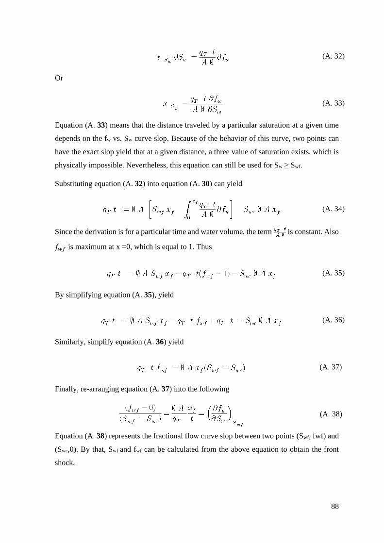
88
(A. 32)
Or
(A. 33)
Equation (A. 33) means that the distance traveled by a particular saturation at a given time
depends on the fw vs. Sw curve slop. Because of the behavior of this curve, two points can
have the exact slop yield that at a given distance, a three value of saturation exists, which is
physically impossible. Nevertheless, this equation can still be used for Sw ≥ Swf.
Substituting equation (A. 32) into equation (A. 30) can yield
(A. 34)
Since the derivation is for a particular time and water volume, the term is constant. Also
𝑓𝑤𝑓 is maximum at x =0, which is equal to 1. Thus
(A. 35)
By simplifying equation (A. 35), yield
(A. 36)
Similarly, simplify equation (A. 36) yield
(A. 37)
Finally, re-arranging equation (A. 37) into the following
(A. 38)
Equation (A. 38) represents the fractional flow curve slop between two points (Swf, fwf) and
(Swc,0). By that, Swf and fwf can be calculated from the above equation to obtain the front
shock.

89
Average saturation
To derive the average saturation behind the front, the same mass balance equation is used
as follows
Injected water = amount of water accumulated – initial water
(A. 39)
By simplifying equation (A. 39) and integrating by part yield
(A. 40)
Substituting equation (A. 32) into equation (A. 40), yield
(A. 41)
Since we derive for a particular time and water volume, the term 𝑞𝑇 𝑡
𝐴 ∅ is constant. Also 𝑓𝑤𝑓
Is maximum at x =0, which is equal to 1. Thus
(A. 42)
By simplifying equation (A. 42), yield
(A. 43)
Similarly, simplify equation (A. 43) yield
(A. 44)
Finally, re-arranging equation (A. 44). yield
(A. 45)

90
Combine equation (A. 38) with (A. 45) to get the complete picture of the front equation.
Thus
(A. 46)
Equation (A. 46) represents Buckley and Leverett's front equation before the breakthrough.
Graphically solution gives the same result for equation (A. 46) by using a tangential line in
the fw vs. Sw curve from Swc.
The following can be found from this equation:
1. The position of the front.
2. Position of any saturation behind the front.
3. Position of the average oil saturation
Before the breakthrough, each of fwf, Swf, and the average saturation are constant with time.

91
After breakthrough
After the breakthrough, the average saturation will change with time.
Mass balance is used to derive the equation after the breakthrough as the following.
Injected water = amount of water accumulated – initial water
(A. 47)
By simplifying equation (A. 47) and integrating, will obtain the following equation
(A. 48)
Substituting equation (A. 32) into equation (A. 48), yield
(A. 49)
Since the derivation is a particular time and particular water volume, the term 𝑞𝑇 𝑡
𝐴 ∅ is constant.
Also 𝑓𝑤𝑓 Is maximum at x =0, which is equal to 1. Thus
(A. 50)
By simplifying the equation (A. 50). Result in the following
(A. 51)
Similarly, simplify equation (A. 51) yield
(A. 52)
Finally, re-arranging equation (A. 52) will obtain

92
(A. 53)
After the breakthrough, the water cut rises suddenly to a value equal to fwf, then with the
production continues, the water cut will rise to value fw1 and increases continuously.

93
Displacement efficiency
Displacement efficiency is the fraction of the oil that has been recovered from the swept
area, and the simple derivation can be done as the following
(A. 54)
Or
(A. 55)
Since
(A. 56)
Substituting equation (A. 56) into equation (A. 55) yield
(A. 57)
Assume that the injection is a perfect process; therefore, the pressure is constant, and Bo
also. Thus
(A. 58)
Since
(A. 59)
Substituting equation (A. 59) into equation (A. 58)
(A. 60)

94
Willhite Areal sweep efficiency correlation
Starting from the concept of Q that expresses the percentage of the water injected volume
to the pore volume and can be derived as the following:
Q at breakthrough can be found as follows
(A. 61)
After breakthrough
(A. 62)
Dividing equation (A. 62) by equation (A. 61) yield
(A. 63)
Integration equation (A. 63) from breakthrough till a particular time after breakthrough will
yield
(A. 64)
Since Dyes and his co-authors developed correlated the areal sweep after the breakthrough
with the ratio of the injected volume at any time to the injected volume at the breakthrough
as the following equation.
(A. 65)
Substitution equation (A. 65) into equation (A. 64) yield
(A. 66)
Where

95
(A. 67)
(A. 68)
This correlation has an appendix of tables that areal sweep efficiency can be found
depending on the value of the fraction 𝑊𝑖
𝑊𝑖𝐵𝑇.
Ei(x) function that appears in the solution of the diffusivity equation appears here as well.
It can approximate by the following
(A. 69)

96
B. APPENDIX B
This appendix contains some tables that are described in this body.
Table B-1.
The history of waterflooding Models.
Date Author(s) Pattern Methods Mobility
Ratio
EA At
Breakthrough
1933
Wyckoff,
Botset and
Muskat
Two-
Spot Potentiometric model 1 52.5
Three-
Spot Electrolytic 1 78.5
Five-
Spot Electrolytic model 1
Seven-
Spot Electrolytic model 1 82
Invert
Seven-
Spot
Electrolytic model 1 82.2
1934
Muskat and
Wyckoff
Five-
Spot Electrolytic model 1
Seven-
Spot Electrolytic model 1 74
1951 Fay and Prats Five-
Spot Numerical 4
1952 Slobod and
Caudle
Five-
Spot
X-ray shadowgraph
using miscible fluids 0.1 to 10
1953 Hurst Five-
Spot Numerical 1
1954 Ramey and
Nabor
Two-
Spot
Blotter-type
electrolytic model 1 to ∞ 53.8 to 27.7
Three-
Spot
Blotter-type
electrolytic model ∞ 66.5
1954 Dyes, Caudle
and Erickson
Five-
Spot
X-ray shadowgraph
using miscible fluids 0.06 to 10
1955 Craig, Geffen,
and Morse
Five-
Spot
X-ray shadowgraph
using immiscible
fluids
0.16 to
5.0
1955 Cheek and
Menzie
Five-
Spot Fluid mapper
0.04 to
10.0
1956 Aronofsky and
Ramey
Five-
Spot Potentiometric model
0.1 to
10.0
1956 Burton and
Crawford
Seven-
Spot Gelatin model
0.33 80.5
0.85 77.0
2.0 74.5

97
Invert
Seven-
Spot
Gelatin model
0.5 77.0
1,3 76
2.5 75
1958 Nobles and
Janzen
Five-
Spot Resistance network 0.1 to 6.0
1958 Paulsell
Invert
Five-
Spot
Fluid mapper
0.319 117
1 105
2.01 99
1959 Moss, White,
and McNiel
Invert
Five-
Spot
Potentiometric ∞ 92
1960 Habermann Five-
Spot
Fluid flow model
using dyed fluids
0.037 to
130
1960 Caudle and
Loncaric
Five-
Spot X-ray shadowgraph
0.1 to
10.0
1961 Bradley, Heller,
and Odeh
Five-
Spot
Potentiometric model
using conductive
cloth
0.25 to 4
1961 Guckert
Seven-
Spot
X-ray shadowgraph
using miscible fluids
0.25 88.1 to 88.2
0.33 88.4 to 88.6
0.5 80.3 to 80.5
1 72.8 to 73.6
2 68.1 to 69.5
3 66 to 67.3
4 64 to 64.6
Invert
Seven-
Spot
X-ray shadowgraph
using miscible fluids
0.25 87.7 to 89
0.33 84 to 84.7
0.5 79 to 80.5
1 72.8 to 73.7
2 68.8 to 69
3 66.3 to 67.2
4 63 to 63.6
1962 Neilson and
Flock
Invert
Five-
Spot
Rock flow model 0.423 110
1968
Caudle,
Hickman and
Silberberg
Four-
Spot
X-ray shadowgraph
using miscible fluids
0.1 to
10.0
Source: (Craig, 1971)

98
Table B-2. Fassihi non-linear regression coefficients.
Coefficient Five-Spot Direct Line Staggered Line
a1 -0.2062 -0.3014 -0.2077
a2 -0.0712 -0.1568 -0.1059
a3 -0.511 -0.9402 -0.3526
a4 0.3048 0.3714 0.2608
a5 0.123 -0.0865 0.2444
a6 0.4394 0.8805 0.3158
Table B-3.
The front advance equations.
Period Q The volume of Injected water
At breakthrough
𝑄𝐴𝐵𝑇 =𝑊𝐴𝐵𝑇
𝑉𝑝=
𝑞𝑡 𝑡𝐵𝑇
𝐴 ∅ 𝑥
=1
(𝜕𝑓𝑤
𝜕𝑆𝑤)
𝑆𝑤𝑓
= 𝑆𝑤̅̅̅̅ − 𝑆𝑤𝑖
=𝑆𝑤𝑓 − 𝑆𝑤𝑖
𝑓𝑤𝑓
𝑊𝑖 = 𝑞𝑡 𝑡 = 𝑉𝑝 (𝑆𝑤̅̅̅̅ − 𝑆𝑤𝑖)
= 𝑉𝑝 ∗𝑆𝑤𝑓 − 𝑆𝑤𝑖
𝑓𝑤𝑓
= 𝑁𝑝 𝐵𝑜
After
breakthrough
𝑄𝑖 =𝑊𝑖
𝑉𝑝=
𝑞𝑡𝑡
𝐴 ∅ 𝑥=
1
(𝜕𝑓𝑤
𝜕𝑆𝑤)
𝑆𝑤2
=𝑆𝑤2̅̅ ̅̅ ̅ − 𝑆𝑤𝑖
1 − 𝑓𝑤2
𝑊𝑖 = 𝑞𝑡 𝑡 = 𝑉𝑝 𝑆𝑤2̅̅ ̅̅ ̅ − 𝑆𝑤2
1 − 𝑓𝑤2
+ 𝑊𝑝 𝐵𝑤
= 𝑁𝑝 𝐵𝑜 + 𝑊𝑝 𝐵𝑤

99
Table B-4.
Material balance results.
Date p Bo
Np
(MMSTB)
GP
Wp
(MMSTB)
WINJ
Rp,
[scf/stb]
Bg Rs Eo Dp Efw F
f/(Eo
+Efw)
Et
Dp/E
O+Ew
f-
Win/e/Et
We
(MMstb)
DDI EDI WDI sum Rf Npr Dpr
12/26
/1996
6174.
32
1.399
21352
0 0 0 0 #DIV
/0!
0.000
141
123.2
5 0 0 0 0 0 0 0 0.00 0
#DIV
/0!
#DIV/
0!
7/13/
1998
5972.
40
1.403
252
0.155
701 0 0 0 0
0.000
146
123.2
5
0.004
038
201.9
2
0.001
542
0.215
683
38.65
071
0.005
5803
13
3618
5.068
8826
738
38.65
0705
9760
0.18 0.000
519
0.111
8666
13
4539.
04599
2
11/7/1999
5728.67
1.408
1266
2
2.552006
0 0.001762
0 0 0.000153
123.25
0.008913
445.65
0.003403
3.547201
288.016
0.012
3159
86
3618
5.0688826
737
288.0
16015934
7
0.40
0.879
8863
61
0.235149
1.13E-01
1.23 0.008507
0.833
6546
36
611.2
02246
4
8/10/
2000
5607.
51
1.410
5497
3.494
2 0
0.002
34 0 0
0.000
157
123.2
5
0.011
336
566.8
1
0.004
328
4.863
659
310.4
957
0.0156641
74
3618
5.068
8826736
310.4
9571
23580
0.51 0.8161703
88
0.218
121
1.04E
-01 1.14
0.011
647
0.8990019
26
567.750042
9
6/25/
2001
5601.
26
1.4106748
4
4.674
84 0
0.002
34 0 0
0.000
157
123.2
5
0.011
461
573.0
7
0.004
376
6.506
704
410.8
524
0.0158370
85
36185.068
8826734
410.85235
73955
0.52 0.6167339
75
0.164
822
7.89E
-02 0.86
0.015
583
1.1897354
13
429.0
48053
4/6/2
002
5394.
20
1.414
816
5.873
829 0
0.002
34 0 0
0.000
163
123.2
5
0.015
602
780.1
2
0.005
957
8.194
487
380.0
91
0.021
559279
36185.068
8826
736
380.09096
6710
7
0.70
0.666
597882
0.178
148
8.54E
-02 0.93
0.019
579
1.101
333836
464.8
473764

100
10/15
/2005
5252.
17
1.417
6566
8.718
031 0
0.002
34 0 0
0.000
168
123.2
5
0.018
443
922.1
5
0.007
041
12.18
084
477.9
727
0.0254843
79
3618
5.068
8826734
477.9
7267
06708
0.83 0.5300389
88
0.141
653
6.80E
-02 0.74
0.029
06
1.3856302
57
370.214214
7
6/20/
2006
5100.
40
1.420
692
9.644
323 0
0.002
34 0 0
0.000
174
123.2
5
0.021
478
1073.
92
0.008
2
13.49
758
454.7
909
0.029
67865
36185.068
8826
735
454.79091
2539
3
0.97
0.557
045876
0.148
87
7.14E
-02 0.78
0.032
148
1.319
044639
389.7
353915
5/2/2
007
5095.
66
1.420
7868
10.77
799 0
0.002
771 0 0
0.000
174
123.2
5
0.021
573
1078.
66
0.008
236
15.08
513
506.0
487
0.029
809643
36185.068
8826
735
506.04872
9067
5
0.97
0.500
627715
0.133
793
6.42E
-02 0.70
0.035
927
1.467
715446
350.2
808965
4/8/2008
5027.40
1.422152
11.968705
0 0.002985
0 0 0.000176
123.25
0.022938
1146.92
0.008758
16.76413
528.9028
0.031
6960
57
3618
5.068
8826
528.9
02789151
0
1.03
0.478
9927
32
0.128011
6.14E-02
0.67 0.039896
1.534
3339
61
335.3
94180
1
10/31/2017
3923.03
1.444
2394
4
29.998888
1726 0.064031
0.033531
57.53547
0.000231
123.25
0.045026
2251.30
0.01719
42.93387
690.0759
0.062
2161
59
3618
5.0688826
733
689.5
36945145
8
2.03
0.367
6027
7
0.098242
4.66E-02
0.51 0.099996
1.989
6336
48
262.660936
5/29/
2018
4041.
04
1.4418791
4
32.26
9707 1939
0.141
596
1.8015222
4
60.08
731
0.000
224
123.2
5
0.042
666
2133.
28
0.016
289
46.21
441
783.8
965
0.0589547
31
3618
5.068
8826734
753.3
3880
10475
2.03 0.3241166
79
0.086
62
8.01E
-02 0.49
0.107
566
2.2549513
42
231.377480
4
6/20/
2018
4201.
70
1.438
666
32.52
5307 1967
0.164
103
1.977
0080
5
60.47
599
0.000
215
123.2
5
0.039
452
1972.
62
0.015
062
46.51
92
853.3
306
0.054
5148
61
3618
5.068
8826733
817.0
6508
47470
2.03
0.297
8824
25
0.079
609
8.29E
-02 0.46
0.108
418
2.452
4402
27
212.2
71140
1
6/22/
2018
4177.
12
1.423
1144
32.54
6029 1969
0.165
629
1.993
25464
60.49
893
0.000
216
123.2
5
0.023
901
1997.
20
0.015
25
46.04
146
1175.
999
0.039
150947
51012.917
1503
883
1125.0866
1604
94
2.03
0.182
346732
0.081
443
8.41E
-02 0.35
0.108
487
2.397
600124
214.7
793207

101
C. APPENDIX C
Decline Curve Analysis Result
Table C-1.
Decline curve wells number
Date Wells Operation
1998-2002 6 Seven is sopped
2002-2003 6, 15
2003-2005 15 6 stopped
2005-2011 15,16
2011-2015 15,16,6 6 retain to production
2015-2016 15,16,6,50,53
2016-2017 15,16,6,50,53,47
16 diesel solvent
2017-2018 15,16,6,50,53,47 15 got solvent stimulation
50 add perf and stimulation
2018-current 15,16,6,50,53,47,69h,101
1. The result for the period 2012-2013
Figure C-1. DC result for the period 2012-2013.

102
2. The result for the period 2013-2014
Figure C-2. DC result for the period 2013-2014.
3. The result for the period 2014-2015
Figure C-3. DC result for the period 2014-2015.

103
4. The result for the period 2015-2016
Figure C-4. DC result for the period 2015-2016.
5. The result for the period 2016-2016 Jun
Figure C-5. DC result for the period Jan-2016 till Jun-2016.

104
6. The result for the period 2016 jun-2017
Figure C-6. DC result for the period 2016 jun-2017.
7. The result for the period 2017-2018
Figure C-7. DC result for the period 2017-2018.

105
8. The result for the period 2018-current
Figure C-8. DC result for the period 2018-current.

106
D. APPENDIX D
Wells Location and Production performance charts
Figure D-1. MB21 formation tops for the study field.

107
Figure D-2. Wellhead pressure map for the sector.
Wells Productivity.
• Well-6
Figure D-3. Well-6 cumulative oil, oil rate, and water rate.

108
Figure D-4. Well-6 production performance curves.
• Well-15
Figure D-5. Well-15 cumulative oil, oil rate, and water rate.

109
Figure D-6. Well-15 production performance curves.
• Well-16
Figure D-7. Well-16 cumulative oil, oil rate, and water rate.

110
Figure D-8. Well-16 production performance curves.
• Well-47
Figure D-9. Well-47 cumulative oil, oil rate, and water rate.

111
Figure D-10. Well-47 production performance curves.
• Well-50
Figure D-11. Well-50 cumulative oil, oil rate, and water rate.

112
Figure D-12. Well-50 production performance curves.
• Well-53
Figure D-13. Well-53 cumulative oil, oil rate, and water rate.

113
Figure D-14. Well-53 production performance curves.
• Well-69H
Figure D-15. Well-69H cumulative oil, oil rate, and water rate.

114
Figure D-16. Well-69H production performance curves.
• Well-116
Figure D-17. Well-116 cumulative oil, oil rate, and water rate.

115
Figure D-18. Well-116 production performance curves.
• Well-36
Figure D-19. Well-36 cumulative oil, oil rate, and water rate.

116
Figure D-20. Well-36 production performance curves.
Figure D-21. Well-36 schematic.

117
E. APPENDIX E
Simulation Results
• Well-116
Figure E-1. Well-116 simulation production performance.
• Well-15
Figure E-2. Well-15 simulation production performance.

118
• Well-16
Figure E-3. Well-16 simulation production performance.
• Well-6s
Figure E-4. Well-6s simulation production performance.

119
• Well-50
Figure E-5. Well-50 simulation production performance.
• Well-53
Figure E-6. Well-53 simulation production performance.

120
• Well-69H
Figure E-7. Well-69H simulation production performance.
• Well-36
Figure E-8. Well-36 injection production performance.

121
• Field production rate
Figure E-9. Field simulation production rate.