faculty of physics and astronomy - mpg.purepubman.mpdl.mpg.de/.../bachelor_schmitz.pdf · faculty...

Faculty of Physics and AstronomyUniversity of Heidelberg

Bachelor thesis

in Physics

submitted by

Frederike Schmitzborn in Mönchengladbach

July 2010

Schottky Diagnostics at the Heavy Ion CoolerStorage Ring TSR

This bachelor thesis has been carried out byFrederike Schmitz

at theMax Planck Institute for Nuclear Physics

under the supervision ofDr. Manfred Grieser and Prof. Dr. Andreas Wolf

Abstract

Schottky diagnostics at the heavy ion cooler storage ring TSR

Schottky diagnostics uses the noise of the beam current in an ion storage ring, calledthe Schottky noise, to determine beam properties such as the momentum spread and thebeam energy. In this thesis, Schottky diagnostics as well as the characteristics of theSchottky pick-up were discussed in theory. In experiments, two different electrostaticpick-ups were used to verify the properties of the Schottky pick-up and the theory ofSchottky diagnostics. For the experiments, a 12C6+ ion beam with an energy of 50 MeVwas used. Signal distortions like amplification with a preamplifier and damping of thesignal through long cables must be taken into account when analyzing the data. Hence,the frequency responses of the utilized amplifiers and cables were measured and usedto adjust the recorded signals. The experimental data was compared to the theoreticalexpectations. Conclusions were drawn to model a new Schottky pick-up that will be inuse in the cryogenic storage ring (CSR).

Kurzfassung

Schottkydiagnose am Schwerionen-Speicherring TSR

Bei der Schottkydiagnose wird das Rauschsignal eines Ionenstrahls in einem Speicherringuntersucht, um Aussagen über Strahlcharakteristika wie die Impulsverteilung und dieStrahlenergie zu machen. In der vorliegenden Arbeit wurde die Schottkydiagnose, sowiedie Eigenschaften des Schottky Pick-ups theoretisch behandelt. In Experimenten mitzwei verschiedenen elektrostatischen Pick-ups konnten die Eigenschaften eines SchottkyPick-ups und die Theorie der Schottkydiagnose bestätigt werden. In den Experimentenwurde ein 12C6+ Ionenstrahl mit einer Strahlenergie von 50 MeV verwendet. Vor derAnalyse der Schottky-Rauschsignale musste berücksichtigt werden, dass das Signal vorder Messung durch Verstärker und das Durchlaufen langer Kabel verändert wird. DerFrequenzgang der verwendeten Kabel und Verstärker wurde daher gemessen und die Sig-nale dementsprechend bereinigt. Nach Analyse der Daten wurden die Ergebnisse derExperimente mit den Erwartungen aus der Theorie verglichen. Schließlich wurden dieErkenntnisse dieser Arbeit verwendet, um einen Schottky Pick-up zu entwerfen, der inZukunft im kryogenen Speicherring (CSR) verwendet wird.

Contents

1 Introduction 1

2 The theory of Schottky noise diagnostics 32.1 Noise spectrum . . . . . . . . . . . . . . . . . . . . . . . . . . . . . . . . . 3

2.1.1 Noise signal of a single ion . . . . . . . . . . . . . . . . . . . . . . . 32.1.2 Noise signal of N monoenergetic ions . . . . . . . . . . . . . . . . . 42.1.3 Noise signal of an ion beam . . . . . . . . . . . . . . . . . . . . . . 6

2.2 Measured spectrum . . . . . . . . . . . . . . . . . . . . . . . . . . . . . . . 72.2.1 Signal of a single ion . . . . . . . . . . . . . . . . . . . . . . . . . . 72.2.2 Signal of the ion beam . . . . . . . . . . . . . . . . . . . . . . . . . 10

2.3 Expected results and applied pick-up geometries . . . . . . . . . . . . . . . 102.4 Determining the beam parameters . . . . . . . . . . . . . . . . . . . . . . . 14

3 Measurement of the Schottky harmonic spectrum 153.1 The experimental setup . . . . . . . . . . . . . . . . . . . . . . . . . . . . . 15

3.1.1 Damping of the signal . . . . . . . . . . . . . . . . . . . . . . . . . 163.1.2 Frequency response of the amplifiers . . . . . . . . . . . . . . . . . 21

3.2 The measurement . . . . . . . . . . . . . . . . . . . . . . . . . . . . . . . . 233.2.1 Measurement with the Schottky pick-up . . . . . . . . . . . . . . . 243.2.2 Measurement with the AM12 pick-up . . . . . . . . . . . . . . . . . 273.2.3 Width of the Schottky bands and momentum spread . . . . . . . . 303.2.4 Increase of the Schottky power at the eigenfrequency of the resonator 31

3.3 The Schottky pick-up length . . . . . . . . . . . . . . . . . . . . . . . . . . 33

4 Outlook and summary 37

1. Introduction

The Test Storage Ring (TSR) has been in operation at the Max Planck Institute forNuclear Physics in Heidelberg since 1988 [1]. The TSR is an experimental facility formolecular, atomic and accelerator physics. With the installation of an electron cooler,the TSR has become the first heavy ion cooler ring. Figure 1.1 shows a sketch of theTSR, which is formed like a rounded square with two 45 dipole deflection magnets ineach corner. Furthermore, two quadrupole doublets are located at each straight sectionand one quadrupole magnet in each corner to focus the beam. The straight sectionsbetween the quadrupoles have a length of 5.2 m, while the circumference of the wholering is 55.42 m. Built into the straight sections are the septum for beam injection andextraction, the electron cooler, the electron target and a diagnostic section with a Schottkypick-up, an ion current monitor and an rf-resonator.The electron cooler produces a cold electron beam at densities of up to 108 cm-3. Underthese conditions a decrease of phase space volume by a factor of > 104 has been achieved.Phase space compression of beams by electron cooling allows beams with an extremelysmall energy spread. The equilibrium values are determined by the balance of the fric-tional force of the cooling electrons and the heating by intra-beam scattering. One ofthe main research areas at the Max Planck Institute for Nuclear Physics (MPIK) is tostudy the interaction of molecular ions and highly charged atomic ions with electrons.For those experiments it is required to be able to determine the properties of the storedion beam. Therefore, we depend on precise diagnostic methods to detect important beamparameters without influencing the beam itself. The momentum spread as well as the rev-olution frequency is easily extracted from the noise spectrum of the beam, the Schottkynoise, which is related to its momentum distribution. In the following Bachelor thesis thecharacteristics of the Schottky harmonic spectrum, as well as the Schottky pick-up usedto measure it, are to be determined and compared with theoretical calculations. Further-more a conceptual design of the Schottky pick-up planned for the Cryogenic storage ring(CSR), which is currently under construction at the MPIK, will be given. The design willbe based on the experimental results about the properties of a Schottky pick-up. Since

1

1 Introduction

Figure 1.1: The test storage ring with its most important elements. The TSR has a circumfer-ence of 55.42 m and the residual gas pressure is 5 · 10−11 mbar

Schottky diagnostics at the CSR will be carried out at very high harmonic numbers ofthe revolution frequency for slow ions, it is necessary to understand the characteristics ofthe whole harmonic spectrum.

2

2. The theory of Schottky noisediagnostics

2.1 Noise spectrum

To measure the revolution frequencey and momentum spread of a stored ion beam, Schot-tky noise diagnostics (see also [2]) is used, meaning that the noise spectrum of the ionbeam current is measured. In order to calculate the noise spectrum, we first consider asingle ion in the storage ring.

2.1.1 Noise signal of a single ion

The current I(t) of a single ion with the charge Q at any given point in a storage ringcan be described as a series of delta pulses (see figure 2.1). Between each of these lies aninterval of T = c0/v, where c0 is the circumference of the ring and v is the velocity of theion. This results in:

Ii(t) = Q∑n

δ(t− nT ) . (2.1)

The phase is arbitrarily set to 0 and varied later in equation (2.7).

Figure 2.1: Ion current of a single ion circulating in a storage ring

3

2 The theory of Schottky noise diagnostics

Because this signal is a periodic function, it can be expressed as a Fourier series:

Ii(t) =a0

2+∞∑n=1

(an cos(n

2π

Tt) + bn sin(n

2π

Tt)), (2.2)

with

ω0 =2π

T(2.3)

an =2

T

T/2∫−T/2

Qδ(t− nT ) cos(n2π

Tt)dt =

2Q

T(2.4)

bn =2

T

T/2∫−T/2

Qδ(t− nT ) sin(n2π

Tt)dt = 0 , (2.5)

which yields:

Ii(t) =Q

T+∞∑n=1

2Q

Tcos(nω0t) . (2.6)

Figure 2.2 shows the related spectrum In of the ion in the storage ring. The spectrumis a series of delta pulses at multiples, called harmonics, of the revolution frequency f0,with f0 = ω0/2π = 1/T .

Figure 2.2: Spectrum of the ion current of a single ion circulating in a storage ring

2.1.2 Noise signal of N monoenergetic ions

The stored ion current of an ion beam that consists of N monoenergetic ions with thecharge Q can be expressed by:

4

2.1 Noise spectrum

I(t) =N∑i=1

(QT

+∞∑n=1

2Q

Tcos(n(ω0t− ϕi))

)(2.7)

=NQ

T+∞∑n=1

N∑i=1

2Q

Tcos(n(ω0t− ϕi)) (2.8)

=NQ

T+∞∑n=1

N∑i=1

2Q

Tcos(

(nω0t) cos(nϕi)− sin(nω0t) sin(nϕi)), (2.9)

with the random phase ϕi, which depends on the time at which the ion arrives at thegiven point in the storage ring. This current can also be written as

I(t) =NQ

T+∞∑n=1

(An cos(nω0t)−Bn sin(nω0t)

), (2.10)

with

An =N∑i=1

2Q

Tcos(nϕi) Bn = −

N∑i=1

2Q

Tsin(nϕi) . (2.11)

To determine the spectral lines we need

A2n =

(2Q

T

)2( N∑i=1

cos(nϕi))2

and (2.12)

B2n =

(2Q

T

)2( N∑i=1

sin(nϕi))2

(2.13)

Because the phases ϕi are randomly distributed, for a large number of ions N, we obtain:

N∑i 6=j

cosϕi cosϕj = 0 andN∑i=1

cos2 ϕi =N

2, (2.14)

and similarly:

N∑i 6=j

sinϕi sinϕj = 0 andN∑i=1

sin2 ϕi =N

2, (2.15)

which yields:

A2n =

(2Q

T

)2N

2= 2N

(QT

)2

and (2.16)

B2n = 2N

(QT

)2

. (2.17)

5


From this, we can conclude that the spectral lines of a monoenergetic beam are:

In =√A2n +B2

n (2.18)

=2Q

T

√N (2.19)

at frequencies n · ω0. The spectral power is correspondingly:

I2n =

(2Q

T

)2

N . (2.20)

2.1.3 Noise signal of an ion beam

If we observe the spectrum of a single ion with the revolution frequency f0,1, we get aseries of delta pulses. A second ion with a different frequency f0,2 renders a series of deltapulses that are shifted from those of the first ion.

Figure 2.3: Spectrum of two ions with different revolution frequencies f0,1 and f0,2

The spectral distance between the delta pulses from the two different ions is given by(f0,1 − f0,2)n. This means that the higher the harmonic number, the further apart thetwo pulses are. How far apart they are is also dependent on the difference between therevolution frequencies and therefore dependent on the difference in velocity (or momen-tum) of the ions. For many ions, the delta pulses form a Schottky band with a certainheight and width, the width of which is connected to the momentum spread of the ions.

6

2.2 Measured spectrum

Figure 2.4: Spectrum of an ion beam. Schottky bands form at harmonics of the averagerevolution frequency f0

The width of the nth Schottky band is given by ∆fn = n∆f0, where ∆f0 depends on themomentum spread ∆p of the ion beam:

f0

∆f0

=1

η

p

∆p. (2.21)

η is the slip factor of the storage ring and describes the dependency of the average revo-lution frequency f0 on the ion momentum p. In the standard mode of the TSR, η = 0.89.The revolution frequencies of an ion beam with an energy spread can be described bya distribution function D(f0) = dN/df0 . Therefore, the spectral power changes into aspectral power density:

dI2n

df=

(2Q

T

)2 dN

df=(2Q

T

)2

D(f0) with f = n · f0 . (2.22)

The power of each Schottky band remains constant:∫dI2

n

df0

df =(2Q

T

)2

N . (2.23)


2.2.1 Signal of a single ion

To detect the ion beam without influencing the beam itself a Schottky pick-up is used.Figure 2.5 shows a sketch of a simple Schottky pick-up, which is a conductive tube aroundthe ion beam. In the diagram, C describes the capacity of the pick-up and the cable thatconnects the pick-up with a preamplifier plus the input capacity of the preamplifier itself.R describes the input resistance of the preamplifier.

7


Figure 2.5: Sketch of a Schottky pick-up including its capacitance C and the resistance R fromthe preamplifier that is used to increase the signal.

The current of a single ion moving through a storage ring at the entrance of the tube canbe described by:

Ii(t) = Q∑n

δ(t− nT ) . (2.24)

Whereas the current at the exit of the tube is given by

Ii,a(t) = Ii(t−∆t) = Q∑n

δ(t− nT + ∆t) , (2.25)

where ∆t is the flight time through the pick-up:

∆t =L

v, (2.26)

with L being the length of the pick-up and v the velocity of the ions.

As with any periodic signal, the currents can be expressed in a Fourier series (see also(2.2)). For the current entering the pick-up we obtain:

Ii(t) =a0

2+∞∑n=1

(an cos(n

2π

Tt) + bn sin(n

2π

Tt)), (2.27)

8


with the Fourier coefficients

an =2

T

T/2∫−T/2

Qδ(t− nT ) cos(n2π

Tt)dt =

2Q

T(2.28)

bn =2

T

T/2∫−T/2

Qδ(t− nT ) sin(n2π

Tt)dt = 0 . (2.29)

at frequencies ω0 = 2π/T , which yields

Ii(t) =Q

T+∞∑n=1

2Q

Tcos(nω0t) . (2.30)

The Fourier series of the current leaving the pick-up is given by

Ii,a(t) =a0

2+∞∑n=1

(an cos(n

2π

Tt) + bn sin(n

2π

Tt))

(2.31)

with the Fourier coefficients

an =2

T

T/2∫−T/2

Qδ(t− nT + ∆t) cos(n2π

Tt)dt =

2Q

Tcos(nω0

L

v) (2.32)

bn =2

T

T/2∫−T/2

Qδ(t− nT + ∆t) sin(n2π

Tt)dt = −2Q

Tsin(nω0

L

v) , (2.33)

which yields:

Ii,a(t) =Q

T+∞∑n=1

(2Q

Tcos(nω0

L

v) cos(nω0t)−

2Q

Tsin(nω0

L

v) sin(nω0t)

). (2.34)

The current that flows into the measuring RC circuit is given by ∆Ii(t) = Ii(t)− Ii,a(t),the difference between the exit and the entrance current:

∆Ii(t) =2Q

T

∞∑n=1

((1− cos(ωn

L

v)) cos(ωnt)− sin(ωn

L

v) sin(ωnt)

). (2.35)

If we look at the amplitude ∆Ii of the current at the frequencies ωn, we can see that thespectrum of the current that flows into the circuit from a single ion is:

∆Ii(ωn) =2Q

T

√(1− cos(ωn

L

v))2

+ sin2(ωnL

v) (2.36)

=2√

2Q

T

√1− cos(ωn

L

v) . (2.37)

9


As seen in figure 2.5, the Schottky pick-up can be described as a capacity C with a parallelresistance R from the input resistance of the preamplifier. The impedance Z of the systemis:

1

Z=

1

R+ iωnC . (2.38)

Therefore the voltage induced by one single ion is given by

Ui(ωn) = |Z|∆Ii(ωn) =R√

1 + ω2nC

2R2

2√

2Q

T

√1− cos(ωn

L

v) . (2.39)

2.2.2 Signal of the ion beam

Now we consider the signal of N Ions with the charge Q interacting with the tube. Theinduced voltage in the measurement circuit is the same for every ion, however, each ionhas a different phase (see also equation (2.7)).

U(ωn) =N∑i=1

Ui(ωn) cosϕi (2.40)

Because the phases ϕi are randomly distributed, the signal U(ωn) of the whole beamaverages to zero over time. Therefore we observe the Schottky power, which is defined as:

P0(ωn) =( N∑i=1

Ui(ωn) cosϕi

)2

(2.41)

As was shown in equation (2.14), for randomly distributed phases ϕi and a large numberof ions N , we obtain: ( N∑

i=1

cosϕi

)2

=N

2(2.42)

Ui(ωn) is equal for all ions, so the Schottky power at harmonic numbers n is given by

P0(ωn) =N

2U2i (ωn) (2.43)

=4NQ2

T 2

R2

1 + ω2nC

2R2

(1− cos(ωn

L

v)). (2.44)

2.3 Expected results and applied pick-up geometries

The Schottky pick-up that is currently used in the TSR is not a closed tube as we pre-viously assumed in our calculations. The existing Schottky pick-up is made up of four 4

10


cm wide conduction strip lines, each located at about 8 cm from the center of the beampath in opposing corners.

Figure 2.6: Sketch of the Schottky pick-up of the TSR

Because of this arrangement we can treat the voltage signal that is induced on one stripline of the pick-up as proportional to one that we would get if we had a closed tube,with a scaling factor κ, where κ is the ratio between the width of one strip line and thecircumference of a tube with a radius which corresponds to the distance of one strip lineto the beam center:

κ =width of one strip linecircumference of tube

. (2.45)

Because the power is proportional to the square of the voltage P ∼ U2, the power wemeasure with one strip line of our pick-up is proportional to κ2:

P (ωn) = κ2 P0(ωn) . (2.46)

The Schottky pick-up currently in use at the TSR has the following properties

Length L = 46.2 cm Capacity C = 68 pF

11


A 12C 6+ beam with the energy E = 50.4 MeV, as used in the experiment, has a revolutionfrequency of about f0 = ω0/2π = 512 kHz. The circumference of the TSR is c0 = 55.42 m.

Figure 2.7: Expected Schottky power harmonic spectrum for a 50 MeV 12C 6+ ion beam usinga preamplifier with 50 Ω input resistance on one strip line of the Schottky pick-up.

Figure 2.8: Expected Schottky power harmonic spectrum for a 50 MeV 12C 6+ ion beam usinga preamplifier with 1 MΩ input resistance and an additional capacitance of 50 pF on one stripline of the Schottky pick-up.

The experiment was conducted with an ion current of I = 20 µA and a preamplifier withan input resistance of R = 50 Ω. The expected result for the measured power at different

12


harmonic numbers n is:

P (n) = κ2 4

T

IQR2

1 + n2ω2oC

2R2

(1− cos(n2π

L

c0

)). (2.47)

If the experiment is carried out with a preamplifier with an input resistance of 1 MΩ, thesignal at lower frequencies is not surpressed (see figure 2.8).

Another pick-up that is used in the measurements is the AM12 position pick-up. It is adiagnostic tool in the TSR that allows us to determine the position of the stored ion beam.It consists of two parts, the horizontal pick-up, to determine the horizontal beam positionand the vertical pick-up to determine the vertical beam position (see figure 2.9). For themeasurement, only the vertical pick-up was used, which is a tube of 8.6 cm length and10 cm radius with a slit that divides it diagonally to measure the location of the beam. Itscapacitance, including the cables which connect it to the amplifier, is C = 176 pF. Usingit as a pick-up to measure the Schottky harmonic spectrum, both parts of the verticalpick-up were connected. As the vertical pick up is a closed tube, except for the negligiblediagonal slit, the theoretical value for κ is 1.

Figure 2.9: Sketch of the AM12 position pick-up in side view. Only the vertical pick-up wasused in the measurements.

13


2.4 Determining the beam parameters

For precision experiments in molecular and atomic physics at the TSR it is extremelyimportant to determine the properties of the ion beam, most of all the energy and themomentum spread. To determine those parameters, we measure the width of the Schottkyband ∆fn and the center frequency fn at a certain harmonic n.From the frequency fn we are able to determine the revolution frequency and from thatthe velocity of the beam:

f0 =fnn

v = f0 · c0 ,

with the circumference of the ring, c0. The kinetic energy of ions with the mass m is givenby

E = (γ − 1) mc2 with γ =1√

1− (vc)2. (2.48)

The momentum spread can be determined by:

∆p =1

η

p

fn∆fn with p = mv , (2.49)

where η = 0.89 in the standard mode of the TSR.

14

3. Measurement of the Schottkyharmonic spectrum

In this chapter the measurements of Schottky harmonic spectra performed with differentexperimental setups are presented and compared to the theory of Schottky diagnostics.The measurements were made with two electrostatic pick-ups of different length anddesign, using a 12C 6+ ion beam with an energy of 50 MeV. The signals from the pick-ups are amplified using one of three different amplifiers. The preamplifiers that are usedare shown in the table below, with their input resistance R and input capacity C. Theshort name is the name by which the amplifiers will be referred to when describing themeasurements.

Amplifier Short name R [Ω] Frequency range Gain [dB] C [pF]

Miteq Miteq 50 1 - 100 MHz 46 ∼ 0

NF SA-230F5 NF 50 Ω 50 100 kHz - 100 MHz 44 ∼ 0

NF SA-220F5 NF 1 MΩ 106 400 Hz - 140 MHz 40 ∼ 50

The NF 1 MΩ amplifier needed to be repaired before, so the actual values for the inputresistance and capacitance might vary from those provided by the manufacturer. Fouridentical Miteq amplifiers are available for measurements with all four strip lines of theSchottky pick-up.

3.1 The experimental setup

After being amplified the signal is conveyed to the control desk by an approximately100 m long double screened cable. At the control desk a Tektronix RSA 3303A spectrumanalyzer is used to record the spectrum of the signal.

15

3 Measurement of the Schottky harmonic spectrum

Figure 3.1: Experimental setup for the measurement of the harmonic spectrum. The signalsfrom the Schottky pick-up are amplified and sent back to the control desk to be measured by aspectrum analyzer.

In this setup, the frequency response of the signal is mainly altered by the amplifier andby the 100 m long cable between the amplifier output and the control desk. To be ableto compare the signal to the theoretical values we must first correct the signal based onthe frequency response of both the cable and the amplifier.

3.1.1 Damping of the signal

The damping of an rf-signal flowing through a cable can largely be described by twoprocesses, resistive losses and losses in the dielectric. A cable can be represented by theschematic diagram seen in figure 3.2.The resistance R′, with R′= R/length, can be derived from the skin effect. An alternat-ing current flowing through a cylindrical conductor causes eddy currents that produce acountervoltage inside the conductor, which leads to the current being pushed to the skinof the conductor, thereby reducing the conducting cross section. Therefore, the resistanceof a cable to an alternating current is equal to the resistance of a hollow tube with wallthickness δ (also called skin depth) to a direct current. The resistance to a current is

16


Figure 3.2: Schematic diagram of a cable, with capacity per unit length C ′, inductivity perunit length L′, resistance per unit length R′ and leakage conductance per unit length G′.

given by

R′ =ρ

A, (3.1)

where ρ is the resistivity of the conductor and A is the area of the cross section. Thecross sectional area in this case is given by

A = (D − δ)δπ ≈ Dδπ (3.2)

where δ is the thickness of the conducting layer caused by the skin effect and D is thediameter of the cable.

Figure 3.3: Schematical cross section of a cable with diameter D and skin depth δ.

The skin depth δ is given by [3]

δ =1

√πµσ

1√f

(3.3)

where µ is the permeability and σ the electrical conductivity of the material and f is thefrequency of the signal flowing through the cable. The resistance of the cable induced bythe skin effect can thus be expressed by:

R′ =ρ

Dπ

√πµσ

√f ∼

√f (3.4)

17


The leakage conductance G′ describes the losses in the dielectric due to the quick changesof the electric field. G′ is proportional to the frequency f of the current flowing throughthe cable [4]:

G′ ∼ f . (3.5)

The voltage U along the cable can be described by the wave equation

d2U(z)

dz2= γ2 U(z) , (3.6)

with z being the position along the cable and

γ =√

(R′ + iωL′)(G′ + iωC ′) = α + iβ , (3.7)

where α is the damping coefficient and β is a phase coefficient [4].The general solution for this equation is:

U = U0e−γz + U1e

γz . (3.8)

As the cable is closed with its characteristic wave impedance of 50 Ω, there is no reflectioninside the cable, so only the signal in one direction remains:

U = U0e−γz . (3.9)

Therefore the ratio of the voltage U after a certain length to the initial voltage U0 can bedescribed by:

ln

∣∣∣∣ UU0

∣∣∣∣ = −α · z , (3.10)

where α is given by [4]

α =R′

2

√C ′

L′+G′

2

√L′

C ′(3.11)

at high frequencies.Using equation (3.10), the damping xD of a cable with the length z is given by

xD = 20 log

∣∣∣∣ UU0

∣∣∣∣ = −20 log(e) · α · z ∼ α . (3.12)

Therefore the fit function that was used to characterize the measured damping of a cableis:

xD = C1f + C2

√f , (3.13)

18


with the fit parameters C1 and C2.

Ten new double shielded cables of about 100 m length were installed between the TSRand the control desk (cables No. 1 to No. 10). To determine the damping of the cables aHewlett Packard 4396A network analyzer was used. The cables are identical and shouldtherefore have the same damping. Nevertheless, the damping of each one was determinedto confirm this.

Figure 3.4: Experimental setup to measure the damping of the cables between the TSR andthe control desk.

First, the damping of cables No. 1 - No. 3 was determined. To do this, an alternatingvoltage from the output of the network analyzer was applied to cable No. 1. At the otherend the cable was directly connected to cable No. 2 and the voltage was sent back to theinput of the network analyzer via cable No. 2 (see figure 3.4).

The frequency response of this setup was recorded and afterwards repeated with cablesNo. 1 and 3 and No. 2 and 3, resulting in three equations for the damping, where xD,ij

19


describes the total damping of cables i and j:

xD,12(f) = xD,1(f) + xD,2(f) (3.14)

xD,13(f) = xD,1(f) + xD,3(f) (3.15)

xD,23(f) = xD,2(f) + xD,3(f) (3.16)

This allows us to calculate the damping of each of the three cables xD,1(f), xD,2(f),xD,3(f) from the measurement of xD,12(f), xD,13(f), xD,23(f) (see figure 3.5) by solvingthe equation system (3.14) - (3.16). Afterwards, cables No. 4 - No. 10 were measuredtogether with cable No. 1 to determine their damping:

xD,i(f) = xD,i1(f)− xD,1(f) (3.17)

Figure 3.5: Measurement of the damping of cables No. 1 and 2, xD,12(f), cables No. 1 and 3,xD,13(f) and cables No. 2 and 3, xD,23(f).

The equation system (3.14) - (3.16) and equation (3.17) was solved for each frequencymeasuring point, the damping for each cable is shown in figure 3.6.

20


Figure 3.6: Damping of the 100 m double screened cables No. 1 to No. 10.

It is evident that the cables all have the same damping. Using the fit function fromequation 3.13 to find a fit for the measuring points results in:

xD(f) = − 0.0093 f − 1.290√f (3.18)

Where f is the frequency in MHz. The result is shown in figure 3.7.

Figure 3.7: Damping of cable No. 10 and the fit through the data points.

3.1.2 Frequency response of the amplifiers

Another component that alters the signal is the amplifier used in the setup. The frequencyresponse of the amplifiers is detected using the same network analyzer that registered the

21


damping of the cables. To prevent reflections along the cables, a 50 Ω resistance wasadded parallel to the input resistance of the NF 1 MΩ amplifier, while measuring itsfrequency response.

Figure 3.8: Setup to measure the frequency response of the amplifiers. For the NF 1 MΩ

amplifier a resistance is added to avoid reflections.

A polynomial function was used to fit the data. Figure 3.9 shows the frequency responseof one of the amplifiers, the NF 50 Ω, as an example.

Figure 3.9: The measured frequency response of the NF 50 Ω amplifier and the fit through thedata points, using a piecewise polynomial function.

22

3.2 The measurement

3.2 The measurement

The spectrum analyzer Tektronix RSA 3303A was used to measure the Schottky harmonicspectra. For this, the power of the Schottky band at each harmonic number was measured.The power that is being recorded is measured across a certain resolution bandwidth, whichmust be taken into account when analyzing the data. To obtain a spectral power density,the power is divided by the resolution bandwidth. Figure 3.10 shows the power signalof the Schottky band at the 60th harmonic of the revolution frequency, measured withthe spectrum analyzer in the setup shown in figure 3.1, using a 50 MeV 12C 6+ ion beam(I = 20 µA) and using one strip line of the Schottky pick-up. The spectrum that is shownhas not been corrected for the amplification and the damping of the cables.

Figure 3.10: The spectral power density of the Schottky band at the 60 th harmonic, measuredwith one strip line of the Schottky pick-up, the NF 50 Ω amplifier and an ion current of I = 20µA, not yet corrected for amplification and damping.

A Gaussian function was used to fit the data:

P ′(f) =A√2πσ

exp

(−(f − f0)2

2σ2

)+B (3.19)

The fit parameter A describes the integral over the Gaussian function and represents thetotal power of one Schottky band. The power from each Schottky band is recorded andafterwards corrected using the frequency response function from the damping of the cableand the amplifier. The corrected power of each Schottky band at the different harmonicsis then plotted against the harmonic number n (see figure 3.11), resulting in the harmonicspectrum.

23


3.2.1 Measurement with the Schottky pick-up

The Schottky harmonic spectrum measured with one strip line of the Schottky pick-upand the NF 50 Ω amplifier is shown in figure 3.11. It shows the power in each Schottkyband as a function of the harmonic number of the revolution frequency f0 = 512 kHz fora 50 MeV 12C 6+ ion beam with a current of I = 20 µA.

Figure 3.11: Harmonic spectrum of the 12C 6+ ion beam, measured with one strip line of theSchottky pick-up and the NF 50 Ω amplifier.

The power of the Schottky bands was corrected for the amplification and the damping ofthe cable and plotted against the harmonic number n. The function that was used to fitthis data was described in chapter 2, equation (2.47):

P (n) = κ2 4f0IQR2

1 + 4π2n2f 2oC

2R2

(1− cos(n2π

L

c0

))

(3.20)

The values for the input resistance of the amplifier R = 50 Ω and the capacity of thepick-up and amplifier C = 68 pF are all known, as are the length of the pick-up L andthe circumference of the TSR c0. The measurement was carried out with a 20 µA carbonbeam with the charge Q = 6 · e+ and the revolution frequency f0 = 512.4 kHz The datawas fitted with the remaining fit parameter κ which was then compared to the theoreticalvalue

κtheo =width of one strip linecircumference of tube

≈ 0.08 . (3.21)

The κ obtained by the data fit is κ = 0.33.

24

3.2 The measurement

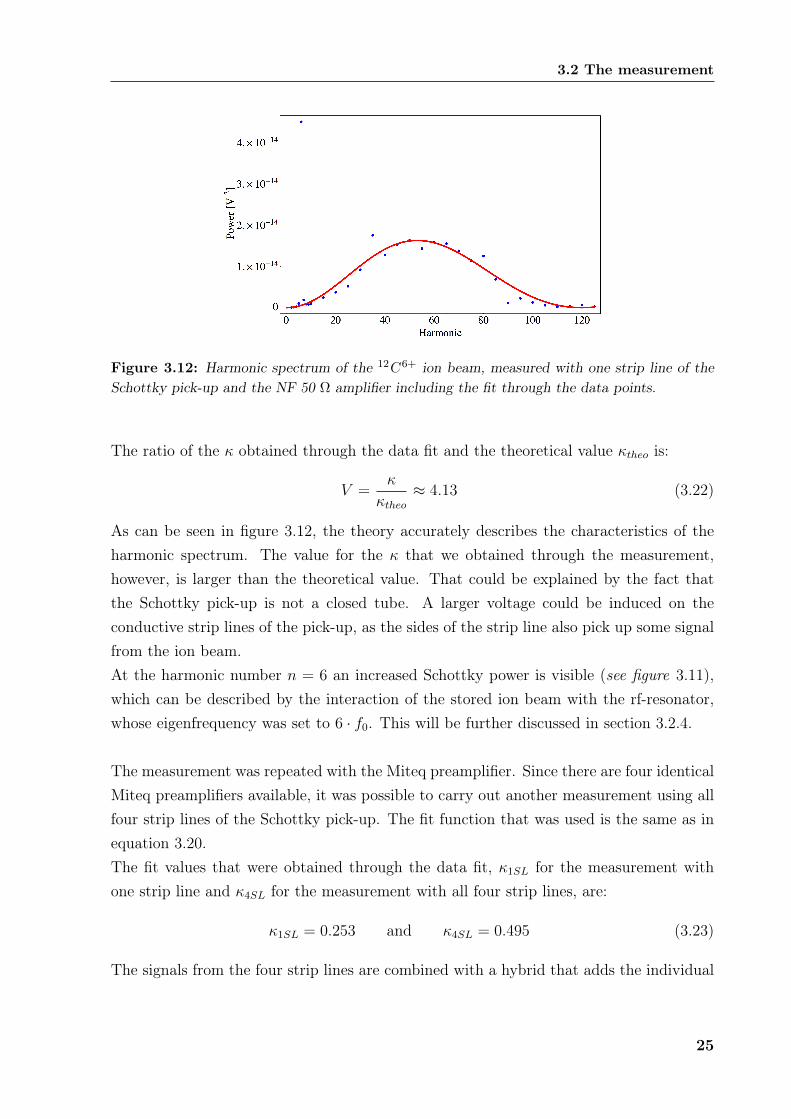
Figure 3.12: Harmonic spectrum of the 12C 6+ ion beam, measured with one strip line of theSchottky pick-up and the NF 50 Ω amplifier including the fit through the data points.

The ratio of the κ obtained through the data fit and the theoretical value κtheo is:

V =κ

κtheo≈ 4.13 (3.22)

As can be seen in figure 3.12, the theory accurately describes the characteristics of theharmonic spectrum. The value for the κ that we obtained through the measurement,however, is larger than the theoretical value. That could be explained by the fact thatthe Schottky pick-up is not a closed tube. A larger voltage could be induced on theconductive strip lines of the pick-up, as the sides of the strip line also pick up some signalfrom the ion beam.At the harmonic number n = 6 an increased Schottky power is visible (see figure 3.11),which can be described by the interaction of the stored ion beam with the rf-resonator,whose eigenfrequency was set to 6 · f0. This will be further discussed in section 3.2.4.

The measurement was repeated with the Miteq preamplifier. Since there are four identicalMiteq preamplifiers available, it was possible to carry out another measurement using allfour strip lines of the Schottky pick-up. The fit function that was used is the same as inequation 3.20.The fit values that were obtained through the data fit, κ1SL for the measurement withone strip line and κ4SL for the measurement with all four strip lines, are:

κ1SL = 0.253 and κ4SL = 0.495 (3.23)

The signals from the four strip lines are combined with a hybrid that adds the individual

25


power signals. The ratio between the power signals is given by the ratio of κ24SL and κ2

1SL:

r =κ2

4SL

κ21SL

= 3.89 (3.24)

which comes very close to the expected value of r = 4.The theoretical value for κ4SL is given by

κ4SL,theo =4 · width of one strip line

circumference of tube≈ 0.32 , (3.25)

so the ratio between the theoretical and the experimental value is:

V =κ4SL

κ4SL,theo

≈ 1.55 (3.26)

As with the measurement with one strip line and the NF 50 Ω amplifier, this is slightlylarger than expected. This could again be explained by a larger voltage being induced onthe sides of the strip lines, as the pick-up is not a closed tube.

Figure 3.13: Schottky harmonic spectra, measured with one and four strip lines of the Schottkypick-up, using four identical Miteq amplifiers.

The measurement was once more repeated with the NF 1 MΩ amplifier. The fit functionis the same as before, the only difference being the input resistance of the amplifier, nowR = 1 MΩ, and the added input capacitance of approximately 50 pF, which results in anoverall capacitance of C = 118 pF.As can be seen in figure 3.14, the fit does not quite match the data points. There areseveral increases of the Schottky power along the harmonic spectrum.These increases can be explained by the pick-up not being a pure capacitance at higherfrequencies, as was assumed in the theory, but also an inductance. This causes the pick-up to be resonant and have self-oscillations, increasing the Schottky power at certain

26

3.2 The measurement

frequencies. This could also explain the slight increases in power in the measurementwith the NF 50 Ω amplifier that can be seen at the 35th harmonic in figure 3.12.

Figure 3.14: Schottky harmonic spectrum measured with one strip line of the Schottky pick-upand the NF 1 MΩ amplifier including the fit through the data points.

The κ that was obtained through the fit is κ = 0.22. This time the ratio of measured andtheoretical κ is:

V =κ

κtheo≈ 2.8 . (3.27)

This deviation from the values for the NF 50 Ω amplifier could be explained by the factthat the NF 1 MΩ amplifier had to be repaired before and the input impedance mighttherefore not be 1 MΩ anymore. Also, the input capacitance of the preamplifier is onlyapproximately known and might also have been changed during the reparations. An inputcapacitance of C = 106 pF would result in the same ratio V = 4.13 as the measurementwith the NF 50 Ω amplifier.

3.2.2 Measurement with the AM12 pick-up

The AM12 pick-up is another pick-up that was used to measure the Schottky harmonicspectrum of a 12C 6+ ion beam with 50 MeV energy and a current of I = 20 µA.The harmonic spectrum that was measured with the NF 50 Ω amplifier is shown in figure3.15.We can see that there is an increase of the Schottky power in the Schottky bands aroundthe 180th harmonic. This increase is even more pronounced in the harmonic spectrumthat was measured with the NF 1 MΩ amplifier (see figure 3.17). Those increases are

27


most probably due to self-oscillations of the system, which could already be observed inthe measurements with one strip line of the Schottky pick-up and the NF 1 MΩ amplifier(see section 3.2.1, figure 3.14). The increased Schottky powers at the harmonics aroundthe self-oscillation were disregarded for the fit, which was performed with the fit functionin equation (3.20).However, as can be seen, the fit does also not match the minimum of the data pointsaround the 300th harmonic. As the position of the minimum of the fit function is definedby the length of the pick-up, another fit was made, this time using the length as a secondfit parameter. The result is shown in figure 3.16.

Figure 3.15: Harmonic spectrum measured with the AM12 pick-up and the NF 50 Ω amplifier.The pick-up length of 8.6 cm was used in the fit, but does not accurately describe the minimumof the spectrum.

The second fit yielded a length of L = 16.2 cm and κ = 0.55. This shows that thelength that best represents the data exceeds the length of the actual pick-up. Also, thetheoretical value is κtheo = 1 for a closed tube, resulting in a ratio:

V =κ

κtheo≈ 0.55 . (3.28)

The measured κ is too small for a closed tube. From this, we can conclude that thereis a required minimum length that a Schottky pick-up needs to have for the theory ofSchottky diagnostics to apply. More thoughts on the pick-up length follow in section 3.3.The measurement that was carried out with the NF 1 MΩ amplifier yielded a length of21.1 cm and κ = 0.36,

V =κ

κtheo≈ 0.36 . (3.29)

28

3.2 The measurement

Figure 3.16: Harmonic spectrum measured with the AM12 pick-up and the NF 50 Ω amplifier.The length was used as a second fit parameter. The increased values for the Schottky poweraround the 180 th harmonic were not considered for the data fit.

Figure 3.17: Harmonic spectrum measured with the AM12 pick-up and the NF 1MΩ ampli-fier. The increase in Schottky power due to self-oscillations around the 180th harmonic is verypronounced.

The deviation from the value of κ obtained through the fit of the measurement with theNF 50 Ω amplifier could be explained by the input resistance and capacitance of the NF 1MΩ amplifier varying from the data provided by the manufacturer, due to the reparationof the amplifier. This was already observed in section 3.2.1, while discussing the resultsfrom the fit of the measurement with one strip line of the Schottky pick-up and the NF1 MΩ amplifier. If we assume an input capacity of C = 106 pF, as was suggested insection 3.2.1, we obtain κ = 0.46, which comes closer to the value from the fit with the

29


NF 50 Ω amplifier, indicating that the NF 1 MΩ amplifier does indeed have a higher inputcapacitance than 50 pF.The lengths from the two fits could differ because the increase in the Schottky power dueto the self-oscillation of the system was much higher in the measurements with the NF 1MΩ amplifier and data points for more harmonics had to be discarded for the fit. Thisprobably resulted in the different values for the pick-up length.The increase in Schottky power around the 180th harmonic is more pronounced in themeasurement with the NF 1 MΩ, because a preamplifier with an input resistance of 1 MΩ

does not dampen the self-oscillation of the pick-up as much as an amplifier with R = 50 Ω.

3.2.3 Width of the Schottky bands and momentum spread

Another important value from the Gaussian fit function in equation (3.19) is the width ofthe distribution, σ, for each Schottky band. This width was plotted against the harmonicnumber. The results from the measurement using four strip lines of the Schottky pick-upand the Miteq preamplifiers are shown in figure 3.18.

Figure 3.18: The width of the Schottky bands measured with four strip lines of the Schottkypick-up and Miteq amplifiers plotted against the harmonic number.

The data was fitted with the function

σn = α · n . (3.30)

Using the fit parameter α and equation (2.49), the relative momentum spread is given by

∆p

p=

1

η

∆fnfn

=1

η

α

f0

with ∆fn = σn . (3.31)

30

3.2 The measurement

The fit parameter that was obtained from the data fit is α = 55.6 Hz, resulting in arelative momentum spread of 1.2 ·10−4 for the electron cooled, 50 MeV 12C 6+ ion beamat a current of I = 20 µA.

3.2.4 Increase of the Schottky power at the eigenfrequency of the

resonator

For acceleration and deceleration of non-relativistic heavy ions on closed orbits in the TSR,variable frequency ferrite loaded resonators are used. The resonance frequency variationis realized by changing the ferrite permeability [5]. The interaction with the resonatorcauses a longitudinal density modulation of the ion beam, which produces an increase inthe signal at the associated frequency. The more precisely the resonator is matched tothe harmonic, the higher the increase.The increase in the Schottky power at the 6th harmonic seen in figure 3.11 is caused bythe interaction of the ion beam with the rf-resonator, where the eigenfrequency of theresonator is set to a multiple n of the revolution frequency f0, in this case n = 6.The resonator eigenfrequency can be adjusted by changing the magnetization of the fer-rites. Figure 3.19 shows the Schottky power of the first ten harmonics with the ferritemagnetization set to 58 A. This resulted in an eigenfrequency of the resonator of 5 · f0,which caused the fifth harmonic in the harmonic Schottky spectrum to be increased. Aferrite magnetization of 65 A changes the eigenfrequency of the resonator to 6 · f0 andincreases the sixth harmonic of the harmonic power spectrum, which can be seen in figure3.20.

31


Figure 3.19: Harmonic spectrum of a 12C 6+ ion beam, measured with one strip line of theSchottky pick-up and the NF 50 Ω amplifier. The Schottky power at n = 5 is increased due tointeraction with the rf-resonator.

Figure 3.20: Harmonic spectrum of a 12C 6+ ion beam, measured with one strip line of theSchottky pick-up and the NF 50 Ω amplifier. The Schottky power at n = 6 is increased due tointeraction with the rf-resonator.

32

3.3 The Schottky pick-up length


As the results from the measurements with the AM12 pick-up indicate (see section 3.2.2),equation (3.20), which describes the Schottky power, does not accurately describe theexperimental results for a pick-up of small length.

In the theory deriving equation (3.20), it was assumed that the ion current of an ion withthe charge Q at the pick-up can be described by a δ-Pulse I(t) = Qδ(t− t0). In a pick-upwith the length L and the capacity C, such an ion current will produce the voltage:

U =

t0+∆t∫t0

I(t′)dt′

C=Q

Cwith ∆t =

L

v(3.32)

with v being the velocity of the ion.

Figure 3.21: The voltage signal produced by a single ion with the charge Q in a pick-up withthe capacity C in our simplified model.

However, it takes a certain rise time trise for the ion to induce a voltage in the pick-up. Ifthe pick-up length is too small, the ion will already have left the pick-up before this risetime has passed and the signal will not reach its maximum.

33


Figure 3.22: The charge on the outside of the pick-up, influenced by the ion, can be describedby a Gaussian charge distribution Λ(s). The width σ of this distribution depends on the velocityof the ion and the radius of the pick-up tube a.

The rise time of the pick-up signal can be estimated by considering an ion moving througha tube with the radius a and length L. The ion induces an image charge on the inside ofthe pick-up wall that is equivalent to its negative charge. Because of charge conservation,the outside surface of the pick-up will have a charge distribution Λ(s), the total chargeof which is equal to the ion charge Q (with s being the position along the pick-up). ForL a, this charge distribution has a Gaussian profile with [6]:

σ =a

γ√

2, with γ =

1√1− v2

c2

andL∫

0

Λ(s)ds = Q (3.33)

where σ is the width of the distribution.If an ion enters the pick-up, the pick-up voltage will increase with the rise time:

trise ≈σ

v. (3.34)

To get the maximum induced voltage U = Q/C on the pick-up, the rise time trise mustbe much smaller than the time that it takes for the ion to pass through the pick-up, ∆t.

∆t trise (3.35)L

v σ

v=

a√2γv

(3.36)

This means that the length of the pick-up tube must be much greater than the radiusL a.

34


In the case of the measurements that were conducted with the AM12 pick-up (a = 10 cm,L = 8.6 cm), the condition L a is not fulfilled, resulting in a much smaller Schottkypower than expected with equation (3.20). This was verified by the measurements dis-cussed in section 3.2.2, which show that the power measured with the AM12 pick-up isonly about 50% of what was expected.

35

4. Outlook and summary

In this chapter the conclusions from the measurements are combined to model the pick-up that will be used in the Cryogenic Storage Ring (CSR), which is currently underconstruction at the MPIK. Also, it is described how the signal can be increased by usinga resonant LC circuit to measure the Schottky niose.

As was discussed in chapter 3.3, the pick-up has to have a certain length. This was alsoverified by the results from the measurements with the AM12 pick-up (see section 3.2.2).The Schottky pick-up that will be used in the CSR will have a radius of a = 5 cm andthe condition L a is fulfilled if a pick-up length of

L = 7 · a = 35 cm (4.1)

is chosen, corresponding to 1 % of the circumference of the CSR, which will be 35 m onceit is completed [7].

To increase the signal of an ion passing through the pick-up tube, an inductance will beconnected parallel to the pick-up capacity, forming a resonant LC circuit (see figure 4.1).As was described in chapter 2, equation (2.37), the spectrum of the current flowing intothe circuit is given by

∆Ii(ωn) =2√

2Q

T

√1− cos(ωn

L

v) (4.2)

The voltage of a single ion at the resonance frequency ωn of the LC circuit is given by

Ui(ωn) =QW

ωnC

2√

2Q

T

√1− cos(ωn

L

v) (4.3)

with QW being the quality factor (Q - factor) of the LC circuit.

37

4 Outlook and summary

Figure 4.1: Sketch of a Schottky pick-up and the resonant LC circuit used to increase theSchottky power. C describes the capacity of the pick-up, R describes the losses of the circuitincluding the input resistance of a preamplifier and L is an inductance that is chosen so thecircuit is resonant at the observed Schottky band.

Now the signal of a single proton stored in the CSR with an energy of E = 300 keV,which corresponds to a revolution frequency of about f0 = 216 kHz, will be estimated.In the frequency range of 200 kHz - 1 MHz an LC circuit can be built with a Q-factorof QW ≈ 1000, if the circuit is cooled down to a temperature of about 4 K. For thecapacitance we assume C = 100 pF; the circumference of the CSR is c0 = 35 m and thelength of the Schottky pick-up L = 35 cm. As is shown in figure 4.2, a proton induces amaximum voltage of 30 nV at low harmonic numbers H = 1 - 10, which corresponds tofrequencies in the range of 200 kHz - 2 MHz.

In summary, it can be said that the signals of a long enough pick-up can be accuratelydescribed by the theory of Schottky diagnostics. Even though the values for the fit pa-rameter κ were larger than expected for the measurements with the strip lines of theSchottky pick-up, the characteristics of the harmonic Schottky spectra match the theory.Deviations from the theory can be explained by increased signals due to self-oscillationsin the system.If the pick-up is too short, the electric charge of the ion beam will not be entirely inducedon the pick-up wall and the signals are smaller than they should be. The measurementsthat were performed with one and four strip lines of the Schottky pick-up show that the

38

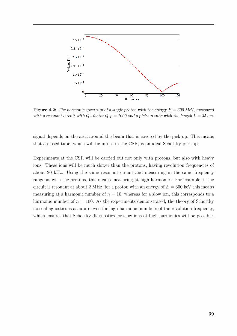
Figure 4.2: The harmonic spectrum of a single proton with the energy E = 300 MeV, measuredwith a resonant circuit with Q - factor QW = 1000 and a pick-up tube with the length L = 35 cm.

signal depends on the area around the beam that is covered by the pick-up. This meansthat a closed tube, which will be in use in the CSR, is an ideal Schottky pick-up.

Experiments at the CSR will be carried out not only with protons, but also with heavyions. These ions will be much slower than the protons, having revolution frequencies ofabout 20 kHz. Using the same resonant circuit and measuring in the same frequencyrange as with the protons, this means measuring at high harmonics. For example, if thecircuit is resonant at about 2 MHz, for a proton with an energy of E = 300 keV this meansmeasuring at a harmonic number of n = 10, whereas for a slow ion, this corresponds to aharmonic number of n = 100. As the experiments demonstrated, the theory of Schottkynoise diagnostics is accurate even for high harmonic numbers of the revolution frequency,which ensures that Schottky diagnostics for slow ions at high harmonics will be possible.

39

List of Figures

1.1 The Test Storage Ring . . . . . . . . . . . . . . . . . . . . . . . . . . . . . 2

2.1 Ion current of a single ion circulating in a storage ring . . . . . . . . . . . . 3

2.2 Spectrum of the ion current of a single ion circulating in a storage ring . . 4

2.3 Spectrum of two ions with different revolution frequencies . . . . . . . . . . 6

2.4 Schottky bands at harmonics of the average revolution frequency . . . . . . 7

2.5 Sketch of a Schottky pick-up . . . . . . . . . . . . . . . . . . . . . . . . . . 8

2.6 Sketch of Schottky pick-up . . . . . . . . . . . . . . . . . . . . . . . . . . . 11

2.7 Expected power spectrum using a 50 Ohm preamplifier . . . . . . . . . . . 12

2.8 Expected power spectrum using a 1 M Ohm preamplifier . . . . . . . . . . 12

2.9 Sketch of AM12 pick-up . . . . . . . . . . . . . . . . . . . . . . . . . . . . 13

3.1 The experimental setup . . . . . . . . . . . . . . . . . . . . . . . . . . . . . 16

3.2 Schematic diagram of a cable . . . . . . . . . . . . . . . . . . . . . . . . . 17

3.3 Cross section of a cable showing skin depth . . . . . . . . . . . . . . . . . . 17

3.4 Experimental setup for damping measurement . . . . . . . . . . . . . . . . 19

3.5 Measurement of the damping . . . . . . . . . . . . . . . . . . . . . . . . . 20

3.6 Damping of cables No. 1 - No. 10 . . . . . . . . . . . . . . . . . . . . . . . 21

3.7 Damping of cable No. 10 and the fit through the data points. . . . . . . . 21

3.8 Experimental setup to measure the frequency response of the amplifier . . 22

3.9 Frequency response of the NF 50 Ohm amplifier . . . . . . . . . . . . . . . 22

3.10 The spectral power density at the 60th harmonic . . . . . . . . . . . . . . 23

3.11 Adjusted harmonic power spectrum for the NF 50 Ohm amplifier . . . . . 24

3.12 Adjusted harmonic power spectrum and fit . . . . . . . . . . . . . . . . . . 25

3.13 Harmonic spectra with fits for the Miteq amplifier, using 1 and 4 strip lines 26

3.14 Harmonic spectrum with fit for the NF 1 M Ohm amplifier . . . . . . . . . 27

3.15 Harmonic spectrum from AM12 and NF 50 Ohm amplifier . . . . . . . . . 28

3.16 Harmonic spectrum from AM12 and NF 50 Ohm amplifier with second fitparameter . . . . . . . . . . . . . . . . . . . . . . . . . . . . . . . . . . . . 29

3.17 Harmonic spectrum from the AM12 pick-up and NF 1 M Ohm amplifier . 293.18 Width of the Schottky bands plotted against harmonic number . . . . . . . 303.19 Increased Schottky power at n = 5 . . . . . . . . . . . . . . . . . . . . . . 323.20 Increased Schottky power at n = 6 . . . . . . . . . . . . . . . . . . . . . . 323.21 Voltage signal in simplified model . . . . . . . . . . . . . . . . . . . . . . . 333.22 Charge distribution on pick-up tube . . . . . . . . . . . . . . . . . . . . . . 34

4.1 Resonant measurement of the Schottky noise signal . . . . . . . . . . . . . 384.2 Schottky spectrum of a single proton . . . . . . . . . . . . . . . . . . . . . 39

Bibliography

[1] E. Jaeschke, D. Krämer, W. Arnold, G. Bisoffi, M. Blum, A. Friedrich, C. Geyer,M. Grieser, D. Habs, H. Heyng, B. Holzer, R. Ihde, M. Jung, K. Matl, R. Neumann,A. Noda, W. Ott, B. Povh, R. Repnow, F. Schmitt, M. Steck, and E. Steffens inProceedings of the first European Particle Accelerator Conference, Rome 1988, p. 365,World Scientific, Singapore, 1989.

[2] D. Boussard, “Schottky noise and beam transfer function diagnostics,” in Cern Ac-celerator School, Advanced Accelerator Physics, Oxford, England, 1985, Proceedings(S. Turner, ed.), vol. II, CERN, Geneva, 1987.

[3] K. Lange and K.-H. Löcherer, eds., Meinke/Gundlach - Taschenbuch der Hochfrequen-ztechnik. Springer Verlag Berlin Heidelberg New York Tokyo, fourth ed., 1986.

[4] H.-G. Unger, Elektromagnetische Wellen auf Leitungen. Dr. Alfred Hüthig VerlagHeidelberg, 1980.

[5] M. Blum, M. Grieser, E. Jaeschke, D. Krämer, and S. Papureanu, “A new type ofacceleration cavity for the Heidelberg test storage ring TSR,” in EPAC 1990, Nice,1990.

[6] A. Hoffmann, “Dynamics of beam diagnostics,” in Cern Accelerator School, BeamDiagnsotics, Dourdan, France, 2008, Proceedings (D. Brandt, ed.), vol. V, CERN,Geneva, 2009.

[7] R. von Hahn, K. Blaum, J. C. López-Urrutia, M. Froese, M. Grieser, M. Lange,F. Laux, S. Menk, J. Varju, D. Orlov, R. Repnow, C. Schröter, D. Schwalm, T. Sieber,J. Ullrich, A. Wolf, M. Rappaport, D. Zajfman, X. Urbain, and H. Quack, “Thecryogenic storage ring project at Heidelberg,” in Proceedings 2008 EPAC08, Genoa,Italy, p. 394, 2008.

Danksagung

An dieser Stelle möchte ich gerne all den Leuten danken, die mir bei der Erarbeitungmeiner Bachelorarbeit geholfen haben.

Mein erster herzlicher Dank richtet sich an Dr. Manfred Grieser, für seine engagierteund lehrreiche Betreuung während meiner Arbeit, ausführliche Erklärungen und diegründlichen Korrekturen während des Schreibens. Ganz herzlich möchte ich mich auchbei Felix Laux bedanken, für die tatkräftige Unterstützung bei vielen Messungen, Math-ematica Tipps, die mir viel Zeit und Nerven gespart haben und zahlreiche beantworteteFragen.

Besonders bedanken möchte ich mich auch bei Prof. Andreas Wolf, der mir ermöglichthat, meine Bachelorarbeit in seiner Arbeitsgruppe zu schreiben und für seine kritischeDurchsicht der Arbeit. Desweiteren danke ich Prof. Klaus Blaum für die Übernahme derZweitkorrektur dieser Arbeit.

Ein weiterer Dank gilt meinen beiden Bürokollegen Wieland Reis und Arthur Schönhalsfür die Tipps beim Schreiben, sowie allen weiteren Mitgliedern der Arbeitsgruppe für einetolle Arbeitsatmosphäre.

Den Operateuren des TSR und der Beschleunigeranlagen möchte ich für ihre Unter-stützung während der Strahlzeiten danken, insbesondere Kurt Horn, der immer zur Stellewar und geholfen hat, wenn etwas nicht funktionierte.

Außerdem geht ein herzlicher Dank an Helen Morrison, die mich bei der englischen Gram-matik und Rechtschreibung vor einigen Fehlern bewahrt hat.

Ein ganz besonderer Dank gilt meiner Familie, die mir mit ihrer finanziellen Unterstützungdieses Studium ermöglichen und mit ihrer moralischen Unterstützung immer den Rückengestärkt haben.

Erklärung:

Ich, Frederike Schmitz, versichere hiermit, dass ich diese Arbeit selbständig verfasst undkeine anderen als die angegebenen Quellen und Hilfsmittel benutzt habe.

Heidelberg, den . . . . . . . . . . . . . . . . . . . . . . . . . . .

. . . . . . . . . . . . . . . . . . . . . . . . . . . . . . . . . . . . . .(Unterschrift)

faculty of physics and astronomy - mpg.purepubman.mpdl.mpg.de/.../bachelor_schmitz.pdf · faculty...

Documents