failure analysis of a 30khz ultrasonic welding

FAILURE ANALYSIS OF A 30KHZ ULTRASONIC WELDING TRANSDUCER

BY

CHRISTOPHER PAUL HAMPTON

THESIS

Submitted in partial fulfillment of the requirements for the degree of Master of Science in Mechanical Engineering

in the Graduate College of the University of Illinois at Urbana-Champaign, 2010

Urbana, Illinois

Adviser:

Professor K. Jimmy Hsia

ii

ABSTRACT

Ultrasonic welding is used across variety of industries to join together thermoplastic materials.

During ultrasonic welding, high frequency mechanical vibrations and compressive pressure are

applied to the plastic materials. This creates intermolecular friction within the plastic which

raises the temperature high enough to reach the melting point. During high volume production in

manufacturing environments, the ultrasonic welding system component which fails most often is

the transducer, which is responsible for creating the vibration. The transducer converts electrical

energy into mechanical energy by means of a polarized piezoelectric PZT (lead zirconate

titanate) polycrystalline ceramic material using high frequency voltage. The transducer is

composed of round PZT disks attached to a titanium machined body by means of a central bolt.

The bolt creates compressive pre-stress which prevents any tensile stresses within the brittle

crystals during vibration and ensures perfect coupling between all components. The

piezoelectric PZT crystals behave according to linear coupled electrical and mechanical

equations. The transducer assembly is vibrated near the parallel resonant frequency to maximize

efficiency and amplitude output.

The purpose of this thesis was to analyze 30 kHz multilayer PZT transducer failures caused by

excessive amplitude (stress) and recommend ways to increase the lifespan. The 30 kHz

transducer design being studied is produced by Herrmann Ultraschalltechnic GmbH and is

currently used in production facilities around the world. Based upon warranty and field data, this

size transducer fails twice as often as the 20 kHz and 35 kHz transducers. The analysis was

based upon studying overall converter design practices and creating a Finite Element model to

understand the stress magnitude and distribution to predict the point of failure. Laboratory

experiments were then performed under high amplitude conditions to increase the stress levels

until failure occurred.

The Finite Element model predicted the current design should be capable of withstanding up to

208% of nominal production level amplitudes (stress) before failure due to uncoupling between

the ceramic crystals and the adjacent conducting plates. During the laboratory experiments the

failures occurred between 179%-244%, however the failure mode did not correlate with the

iii

failure predicted by the Finite Element model. All of the failures during the experiment resulted

from electrical arcing at the inner diameter of the bottom ceramic disks. Furthermore, these

laboratory failure modes were not consistent with those normally observed in production

environments where fracture and shifting of crystals are the dominant modes. We can conclude

that the electrical load used in the experiments did not accurately represent production welding

conditions, which means it could not be used as a comparison against the Finite Element model.

In order to increase the lifespan of the transducer additional testing must be performed. First and

foremost would be new tests which accurately reproduce production welding conditions. Then

these results could be tested against the Finite Element model. Once this was completed, if the

models accuracy was verified, improvements could be made and tested with the Finite Element

model to try and increase the lifespan.

iv

ACKNOWLEDGMENTS I would like to first and foremost acknowledge Professor K. Jimmy Hsia. Not only did he guide

me through the thesis process but through his classes I gained many insights into failure modes

and how to analyze failures. It was not easy to coordinate a thesis via e-mail and telephone,

however he was very accommodating. I would also like to thank an industry expert and

ultrasonic consultant James Sheehan of JFS Engineering Incorporated for many thought

provoking conversations and countless hours of help with ANSYS, a program I had never

worked with before. Ulrich Vogler, an R&D manager at Herrmann Ultraschalltechnic GmbH

played an integral role in designing and executing the transducer experiments necessary to

complete this thesis. Most importantly, I would like to thank my wife for her patience,

understanding and editing skills; I know these past 28 months were not easy…

v

TABLE OF CONTENTS LIST OF TABLES ...................................................................................................................... vii

LIST OF FIGURES ................................................................................................................... viii

CHAPTER 1: Introduction .......................................................................................................... 1

1.1 What is ultrasonic welding ........................................................................................... 1

1.2 Components in an ultrasonic welder........................................................................... 1

1.3 Construction and electrical control of a 30kHz transducer...................................... 3

1.4 Failure modes and lifetime of 30kHz transducer....................................................... 4

1.5 Importance of transducer lifespan .............................................................................. 6

1.6 Tables and Figures ........................................................................................................ 7

CHAPTER 2: Literature review................................................................................................ 11

2.1 Fundamentals of PZT piezoelectric crystals............................................................. 11

2.2 Langevin type piezoelectric PZT transducer design and operation....................... 13

2.3 Modeling transducers with FEA................................................................................ 19

2.4 Tables and figures ....................................................................................................... 22

CHAPTER 3: FEA model of current 30 kHz transducer ....................................................... 28

3.1 Overview ...................................................................................................................... 28

3.2 Modal analysis results................................................................................................. 29

3.3 Harmonic analysis results .......................................................................................... 29

3.4 Static pre-stress analysis results ................................................................................ 30

3.5 Calculated stress limit and safety factor in the piezoelectric crystals.................... 31


CHAPTER 4: Experiment, transducer failure due to excessive amplitude .......................... 51

4.1 Experimental set-up.................................................................................................... 51

4.2 Equipment ................................................................................................................... 52

4.3 Test Procedure ............................................................................................................ 52

4.4 Results .......................................................................................................................... 54


CHAPTER 5: Conclusions ......................................................................................................... 73

5.1 Summary of key points in FEA analysis and experiment results ........................... 73

vi

5.2 Compare results between FEA and experiment ...................................................... 73

5.3 Inaccuracies in FEA analysis and experiment causing deviations in results ........ 75

5.4 Recommendations for additional testing .................................................................. 76


References .................................................................................................................................... 80

Appendix A – Modifying piezoelectric material data to enter into ANSYS...................... 82

Appendix B – Alternate modes of vibration for series and parallel resonance................. 87

Appendix C – Nodal stress calculations for static and dynamic analyses ......................... 89

Appendix D – Raw test data from experiment..................................................................... 93

vii

LIST OF TABLES

Table 3.1 – Material properties used in FEA analysis - (a) Basic mechanical properties of

PZT801, (b) Elasticity matrix for PZT801, (c) Piezoelectric stress matrix for

PZT801, (d) Permittivity matrix for PZT801, (e) Material properties for

beryllium, titanium and steel………………………………………………………. 32

Table 3.2 – modal frequencies under open and closed circuit boundary conditions (yellow

highlighted row is primary mode) – (a) Series modal frequencies, (b) Parallel

modal frequencies…………………………….……………………………………. 33

Table 4.1 – Testing equipment specifications …………………………………………………. 56

Table 4.2 – Baseline amplitude readings at 100% nominal amplitude………………………… 57

Table 4.3 – Impedance plot values before and after failure……………………………………. 57

Table 4.4 – Summary of failure modes………………………………………………………… 58

Table 5.1 – Comparison of impedance between FEA and experimental results………………. 76

Table A.1 – Material properties from manufacturer’s data sheet adjusted for preload………... 83

Table A.2 – Material properties adjusted to account for axis configuration in ANSYS………. 83

Table A.3 – Compliance matrix – (a) Compliance matrix inputs, (b) Stiffness matrix, (c)

Stiffness matrix adjusted for shear terms…………………………………………... 84

Table A.4 – Piezoelectric matrix – (a) Piezoelectric values from manufacturer, (b)

Transposed piezoelectric values, (c) Piezoelectric matrix multiplied by the

stiffness matrix, (d) Final piezoelectric matrix adjusted for shear terms…………... 85

Table A.5 – Permittivity matrix – (a) Permittivity values from manufacturer, (b) Permittivity

values for input to ANSYS ………………………………………………………... 86

Table C.1 – numerical calculations from FEA analysis – (a) Top of disk #1, (b) Bottom of

disk #1, (c) Top of disk #2, (d) Bottom of disk #2, (e) Top of disk #3, (f) Bottom

of disk #3, (g) Top of disk #4, (h) Bottom of disk #4……………………………… 89

Table D.1 – raw data from testing (contained in the next 8 pages, created using larger paper

size to accommodate the amount of information and to improve readability)…….. 94

viii

LIST OF FIGURES

Figure 1.1 – Parts welded with ultrasonics…………………………………………………….. 7

Figure 1.2 – Schematic of vibrating assembly………………………………………………… 8

Figure 1.3 – Diagram of welding fixture and vibrating stack…………………………………. 8

Figure 1.4 – Force build-up mechanism attached to a vibrating stack………………………… 9

Figure 1.5 – Cross section of 30 kHz transducer……………………………………………… 9

Figure 1.6 – Picture of 30 kHz transducer……………………………………………………... 10

Figure 1.7 – Transducer failure due to cracked crystals……………………………………….. 10

Figure 1.8 – Transducer failure due to shifting crystals……………………………………….. 10

Figure 2.1 – Phase diagram of PbZrTi…………………………………………………………. 22

Figure 2.2 – Molecular structure of PZT above and below Curie temperature………………... 22

Figure 2.3 – SEM of PZT showing grains, grain boundaries and voids……………………….. 23

Figure 2.4 – Un-poled and polarized PZT……………………………………………………... 23

Figure 2.5 – Polarized material with various electric charge states…………………………… 24

Figure 2.6 – mass-spring-mass transducer model……………………………………………… 24

Figure 2.7 – stress/strain and displacement along transducer during vibration……………….. 25

Figure 2.8 – Equivalent series and parallel resonance circuits………………………………… 26

Figure 2.9 – Example impedance plot of transducer…………………………………………... 27

Figure 3.1 – 2-D axisymmetric geometry of 30 kHz transducer………………………………. 34

Figure 3.2 – Configuration of polarized PZT crystals for FEA analysis………………………. 34

Figure 3.3 – Morgan Ceramics PZT801 data sheet……………………………………………. 35

Figure 3.4 – Meshed geometry………………………………………………………………… 36

Figure 3.5 – Boundary conditions during modal analysis……………………………………... 36

Figure 3.6 – Series modal vibration plots – (a) fully extended modal shape at series

resonance, (b) fully compressed modal shape at series resonance……..………….. 37

Figure 3.7 – Parallel modal vibration plots – (a) Fully extended modal shape at parallel

resonance, (b) fully compressed modal shape at series resonance………………... 38

Figure 3.8 – Impedance versus frequency plot from 29,000-33,000 Hz……………………… 39

Figure 3.9 – Amplitude versus frequency plot from 29,000-33,000 hertz…………………….. 40

Figure 3.10 – Amplitude versus frequency from 30,650-30,750 hertz………………………… 41

Figure 3.11 – Von Mises stress distribution at 30,700 hertz…………………………………... 42

ix

Figure 3.12 – Von Mises stress distribution at 30,700 hertz, only showing piezoelectric

crystals …………………………………………………………….…………......... 42

Figure 3.13 – Von Mises stress distribution under static load over entire model……………… 43

Figure 3.14 – Von Mises stress distribution under static load at ceramic crystals…………….. 43

Figure 3.15 – Contact pressure over entire model under static load…………………………… 44

Figure 3.16 – Contact pressure at bottom of each crystal under static load…………………… 45

Figure 3.17 – Contact pressure at disk #1 and disk #4………………………………………… 45

Figure 3.18 – Graphs illustrating summing of static and dynamic stresses to calculate total

stress – (a) Static and dynamic loads separated, (b) Static and dynamic loads

combined…………………………………………………………………………… 46

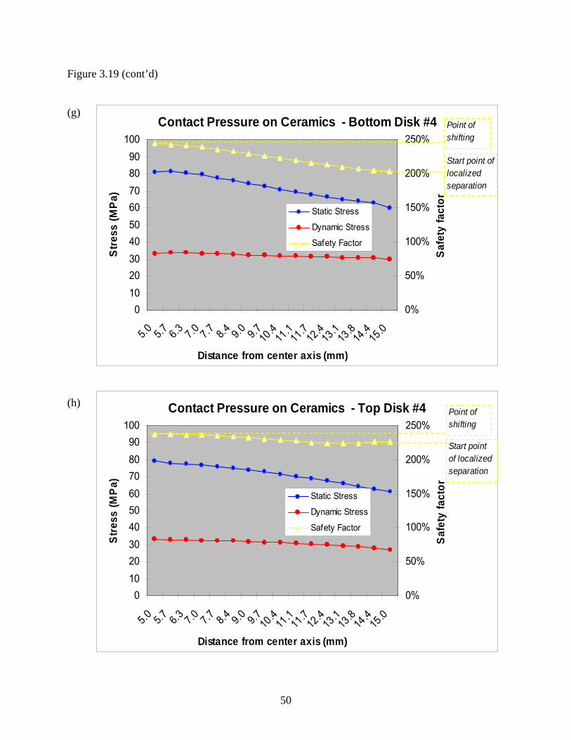
Figure 3.19 – Static and dynamic contact pressure between ceramics including safety factor –

(a) Top of disk #1, (b) Bottom of disk #1, (c) Top of disk #2, (d) Bottom of disk

#2, (e) Top of disk #3, (f) Bottom of disk #3, (g) Top of disk #4, (h) Bottom of

disk #4……………………………………………………………………………… 47

Figure 4.1 – Drive and slave transducer set-up – (a) configuration of vibrating stack for

testing, (b) configuration creating nominal stress values in slave transducer, (c)

alternate configuration to create nominal stress values in slave transducer, (d)

configuration creating 150% overstress in slave transducer……………………….. 59

Figure 4.2 – Picture of vibrating test stack…………………………………………………….. 61

Figure 4.3 – Schematic of overall equipment set-up…………………………………………... 61

Figure 4.4 – Pictures of experimental set-up – (a) Laser vibrometer, electronic load,

vibrating stack, (b) Temperature sensor, generator, computer with DIASIM,

laser vibrometer control cabinet, oscilloscope, (c) Rigid booster mount, slave

transducer, booster, drive transducer, (d) Close-up of vibrating test stack, (e)

Cooling lines, electronic load connections, temperature probe, measuring point

for laser vibrometer………........................................................................................ 62

Figure 4.5 – Typical oscilloscope reading showing amplitude at reflector plate……………… 64

Figure 4.6 – Cycles to failure including amplitude or stress level…………………………….. 64

Figure 4.7 – Typical impedance plot…………………………………………………………... 65

Figure 4.8 – Pictures of converter failures – (a) Transducer #1, (b) Transducer #2, (c)

Transducer #5, (d) Transducer #6, (e) Transducer #7…………………………....... 66

x

Figure 4.9 – DIASIM graphs before and after entering destabilized zone…………………….. 72

Figure 5.1 – Pictures of typical production transducer failure…………………………………. 77

Figure B.1 – Alternate modes of vibration during parallel and series vibration – (a) Series

mode at 54,424Hz, (b) Series mode at 57,659Hz, (c) parallel mode at 55,321Hz… 87

1

CHAPTER 1: Introduction

1.1 What is ultrasonic welding

Ultrasonic welding is one of the most popular technologies used for joining thermoplastic

materials to create an assembly or finished product. It can be applied to amorphous or semi-

crystalline polymers, but not to thermo-sets. Its main advantages include:

• Short weld cycles (can be less than 100miliseconds)

• Localized welding

• Precise melting of only a small area

• No consumable solvents or glues

• Low energy consumption

• Hermetic sealing through contaminated surfaces or interfaces

Ultrasonic welding uses high frequency mechanical vibrations between 20 kHz to 35 kHz

combined with a compressive force to create intermolecular friction within polymers at an

interface. Localized melting occurs at this interface once enough heat has been generated to

reach the melting or glass transition temperature. The polymers melt and diffuse due to breakage

in the secondary molecular bonds, thus allowing previously immobile and separate molecular

chains to intermix and flow together. This process is aided by application of an external force

[1]. Upon removing the ultrasonic vibrations, the temperature rapidly decreases and new

secondary bonds form between molecules containing the previously separate layers of

thermoplastic. The strength of this new bond can almost reach that of the un-bonded material

[1]. The term “ultrasonic” refers to the frequencies used during welding, which are beyond the

range of human hearing but within the ultrasound wave range. Ultrasonic welding is used across

a wide variety of industries including automotive, hygiene, feminine care, food packaging,

electronics and medical devices. Figure 1.1 shows parts commonly welded using ultrasonics.

1.2 Components in an ultrasonic welder

An ultrasonic welding system can be broken into three main areas:

1. The vibrating sub-assembly

2. The fixture

2

3. The force build-up mechanism

The vibrating sub-assembly consists of a generator, high frequency cable and vibrating

transducer/booster/sonotrode. Low voltage and low frequency electricity (typically 230 VAC at

60 Hz) is introduced into the generator where it is transformed through digital circuits into a high

voltage/frequency signal (typically 800-1000VAC at 20,000-35,000 Hz). This high

voltage/frequency electricity is transmitted through the high frequency cable into the transducer

where the electrical energy is transformed into mechanical energy. The transducer vibrates in a

pure axial mode due to its design and the way the electrical signal is controlled. The amplitude

of this longitudinal wave created at the anti-node of the transducer is too low to weld most

materials, thus it must be amplified by a booster. The booster increases the amplitude based

upon the mass ratio between the top and bottom halves along with the efficiency of the metal.

The amplitude can be further increased by the sonotrode, which is also the component used to

contact the part being welded. Figure 1.2 shows the vibrating components and how the parts

interconnect.

The fixture is a rigid stationary structure used to hold the polymer component(s) being welded.

The fixture is typically metal with enough mass and rigidity to dampen the vibrations created by

the sonotrode. This is done to ensure most of the vibrational energy is consumed by the plastic

component and can be used for initiating melt flow. The geometry of this part is also chosen so

that its resonant frequency is far from the vibrating frequency of the sonotrode, thus ensuring it

does not oscillate at high amplitudes during welding. An ideal fixture will dampen all vibrations.

A diagram of a typical stack and welding fixture or anvil for welding two thin plastic films is

shown in figure 1.3.

The force build-up mechanism is used to control the amount of force being applied to the

thermoplastic component(s) during welding. This is typically accomplished with an air cylinder

or stepper motor, which applies a force directly against the vibrating stack. The vibrating stack

is usually mounted on a precision sliding surface to ensure smooth movement. The force must

be high enough to ensure transmission of the energy into the plastics and draw enough power

from the transducer to quickly reach the melting point while forcing the melted surfaces together.

3

Force is one of the most important variables in determining the quality of a weld. Therefore, it

must be carefully controlled to create a consistent weld. Figure 1.4 shows a picture of a typical

force build-up system attached to a vibrating stack.

These components are combined into one assembly or “machine” which can then be used to

weld plastic components.

1.3 Construction and electrical control of a 30kHz transducer

Almost all converters used in plastic ultrasonic welding have the same basic construction. The

differences are minor geometric changes and some material variations. Transducers are

constructed based upon a Langevin type design which is an assembly with polarized

piezoelectric PZT ceramic material sandwiched between two metal cylinders with a bolt in the

middle to hold them together. The most common design variation is a cylindrical ½ wavelength

assembly composed of a metal body with multiple disk shaped PZT crystals and a central bolt to

keep the components in compression at all times. The metal body usually has a mounting

surface at the nodal point where there is zero net vibration or amplitude. The PZT disks are

polarized and oriented so that common polarities face each other, i.e. positive faces positive and

negative faces negative. In between each PZT disk is a copper-beryllium conducting plate where

the electricity is applied via wires. Figures 1.5 and 1.6 shows a cross section and picture of the

30 kHz converter being examined in this paper. The converter studied is designed and

manufactured by Herrmann Ultraschalltechnic GmbH based in Karlsbad Germany (HUG).

The amount of amplitude and power created by the vibrating transducer is controlled

electronically with a power supply or ultrasonic generator. The generator is designed so that the

vibrating assembly maintains the same amplitude at the welding surfaces at all times, regardless

of how much force is being applied to the welded part. The challenge is that the generator has no

direct feedback of the physical displacement inside the PZT ceramics; it can only monitor and

control the voltage, current and frequency. Because amplitude is a function of velocity and

frequency (see equation 1.1 below), the amplitude is kept constant by maintaining the same

frequency and velocity [2].

4

λπ ∗∗= fv 2 (1.1)

The frequency can be directly controlled by the generator, but the velocity can only be controlled

and maintained by varying the current or power according to equation 1.2 shown below.

vFP ∗= (1.2)

In this equation P, is power which is based upon amperage or current and F is the external force

being applied to the vibrating surface. To summarize, the generator maintains the same

amplitude under various welding forces by increasing or decreasing the current/power to

maintain the velocity while simultaneously keeping the frequency constant (or changing it only

fractions of a percent) to satisfy equation 1.1.

1.4 Failure modes and lifetime of 30kHz transducer

There are seven main failure modes for an ultrasonic transducer. These failure modes are based

upon the author’s direct experience for the past 5 years in the field of ultrasonic welding.

1. Fracture of ceramic crystals

Fracture occurs when the crack grows large enough to cause the crystals to separate

into multiple pieces. Even if the separated pieces do not move apart from eachother

the fracture surfaces are no longer perfectly coupled, which allows relative motion

leading to friction and rapid overheating [3]. Poor coupling at the interface causes the

resonant frequency to change, creates unequal electrical properties and allows a short

circuit path for high voltage arcing. Cracks initiate at either pre-existing cracks/voids

or they are formed by tensile loads, impact stresses or shear stresses [4]. Figure 1.7 is

a picture of a converter failure due to cracked PZT crystals.

2. Shifted ceramic crystals

Crystals can be displaced along the plane perpendicular to the axis of symmetry when

compressive pre-stress at two mating surfaces temporarily becomes zero. Once

crystals shift, mechanical forces and moments are no longer symmetric about the

central axis, which creates a bending moment rather than perfectly longitudinal

motion. At this point amplitude distribution is no longer even, power draw increases

5

and internal stresses increase in the crystals. In many cases, shifted ceramic crystals

also lead to fracture. Figure 1.8 shows converter failure due to shifted crystals.

3. Arcing due to short circuit

If the voltage applied to the ceramic crystals is high enough and/or two conducting

surfaces of opposite polarity are close enough, then arcing can occur. This arcing can

cause local depolarization due to very high temperatures and thus possibly initiate

crystal fracture.

4. Fracture of pre-stress bolt

Fracture of the pre-stress bolt occurs when the dynamic tensile stress exceeds the

endurance limit. When this happens the fracture propagates through bolt causing

complete failure, breaking the bolt into 2 pieces. After bolt failure, pre-stress

becomes zero, all transducer components become uncoupled and the transducer will

not operate.

5. Fracture of Beryllium conducting plate at wire connector

A small portion of the Beryllium plate is not compressed between PZT crystals and

protrudes for attachment to the conducting electrical wire. The electrical conducting

wire is connected to the top housing of the transducer body, however the beryllium

plate where it connects is vibrating at the same frequency and magnitude as the PZT

crystals. This protruding section can fatigue due to high frequency flexure and

fracture, causing a loss of electrical power to one set of PZT crystals. This

completely changes the electrical properties of the transducer. The remaining crystals

are forced to carry all remaining power which overloads them and leads to

overheating or fracture. The loose wire created during this failure can also touch

other parts of the transducer and create a short circuit.

6. Fracture in the Titanium body

Fracture in the Titanium body occurs due to crack growth caused by dynamic stresses

which exceed the fatigue limit. As the crack grows, the resonant frequency of the

transducer changes until it is outside permissible operating limits. Alternately, the

cracked surface temperature can overheat the entire transducer.

7. Overheating of PZT crystals

6

Overheating the PZT crystals occurs when the temperature rises close to the Curie

point and de-polarization begins. During depolarization the crystals lose their

piezoelectric properties leading to excessive dynamic stress and fracture (failure #1).

Based upon data collected between 2006-2008, over 80% of recorded transducer failures resulted

from cracked and shifted crystals [5]. These two failure modes will be the focus of this thesis.

The lifespan of a transducer varies widely depending upon the welding application and proper

operation. Based upon the author’s 5 years of field experience visiting customers and repairing

equipment, several generalities can be made:

1. Transducers in low force and/or low power applications last longer than those in high

force and/or high power applications.

2. More welding cycles shorten the lifespan.

3. Properly operated and maintained transducers can vary from as little as 3 months and as

long as 10 years producing tens of millions of welded parts. The average life expectancy

is between 1-3 years. Customers expect a transducer to last at least one year.

Between 2006-2008, the failure rate of 30 kHz transducers varied between 5-15%. This failure

rate is based upon the number of transducers returned for examination compared to the total

number manufactured that same year. Data for the other two sizes produced by HUG (20 kHz

and 35 kHz) show much better life-spans, with failure rates between 4-8% [5].

1.5 Importance of transducer lifespan

The acceptable lifespan and failure rate of an ultrasonic transducer due to defects, is based upon

the expectations of the end users and the nature of ultrasonic applications. Fortunately,

transducer failure does not pose a health risk to an individual. There is no single recordable case

of serious injury due to transducer failure. However, excessive failure rates tarnish a company’s

image and can cause a loss of future business. In addition, there are hard costs associated with

replacing the failed components including the resources wasted to build the original failed part,

the resources to create a new part, the labor to replace the component and process the paperwork

for each of these steps. The customer incurs additional costs in poorly welded products, possible

7

customer liability, loss of production plus labor to troubleshoot and replace the failed

component. It is very difficult to quantify what an ideal lifespan and failure rate should be.

From a customer perspective they should last forever, but in reality the resources needed to

create the “perfect” transducer are limited. As with virtually all engineered products there must

be a balance between the resources available to design and optimize a part counterbalanced by

market demands allowing the product to be competitive and generate revenue. The goal of this

paper is to increase the lifespan and reduce the annual failure of the 30 kHz transducer. This will

be accomplished by investigating the current design through FEA analysis, verifying the

accuracy of the FEA model through laboratory testing and then refining the model to allow for

higher stress levels before failure occurs.

1.6 Tables and Figures

Figure 1.1 – Parts welded with ultrasonics

8

Figure 1.2 – Schematic of vibrating assembly

Figure 1.3 – Diagram of welding fixture and vibrating stack

9

Figure 1.4 – Force build-up mechanism attached to a vibrating stack

Figure 1.5 – Cross section of 30 kHz transducer

Air cylinder creates welding force

Sonotrode vibration

10

Figure 1.6 – Picture of 30 kHz transducer Figure 1.7 – Transducer failure due to cracked crystals

Figure 1.8 – Transducer failure due to shifting crystals

11

CHAPTER 2: Literature review

2.1 Fundamentals of PZT piezoelectric crystals

Piezoelectricity was first discovered in 1880 by Jacques and Pierre Curie. They discovered that

in certain materials an electric charge could be generated by applying a stress. The most well

known material exhibiting this property is quartz. In Greek, the word “piezo” means “to press”.

Therefore, piezoelectricity literally means generating electricity from pressure [6]. The Curies

later confirmed the reverse effect whereby mechanical strain can be generated by applying an

electric charge. In the 1950s more efficient and powerful piezoelectric materials were

discovered, including those in the form of lead zirconate and lead titanate (PZT). These

materials can have a permanent dipole moment and a much higher dielectric constant. They can

be easily manufactured as polycrystalline ceramics, doped with a variety of elements and

polarized [6]. Lead zirconate titanate (PbZr1-x Tix O3) is the material used in the ultrasonic

transducers studied in this paper.

The piezoelectric properties of PZT ceramics are a result of their molecular structure. The most

useful piezoelectric properties are observed when the mole fraction of Ti and Zr are close to 0.5.

PbZr.47 Ti.53 O3 is a common configuration used in industry. Examining the phase diagram in

figure 2.1, it is apparent that multiple crystalline structures can exist near this mole fraction.

This transitional area is called the morphotropic phase boundary (MPB) [7]. Above the Curie

temperature (Tc), the structure is cubic. At this point there is no net dipole due to cubic

symmetry. However once the temperature drops below the Curie point, the structure becomes

tetragonal or rhombohedral. It is this distorted structure that creates an electric dipole moment.

These non-cubic structures have over 14 stable domain configurations at the MPB giving them

great flexibility during polarization [7]. Figure 2.2 shows the structure above and below the

Curie temperature.

Unit cells in PZT crystals combine to form domains. Because they are polycrystalline materials,

there are grain boundaries and voids formed during manufacturing, which separate these

domains. Figure 2.3 shows an SEM image of a typical PZT under high magnification [8]. The

12

individual grains, grain boundaries and voids are clearly visible. The material properties are

dependent on grain size, grain boundary thickness as well as the size and number of voids.

These properties are all controlled during the manufacturing process and must be consistent in

order to maintain consistent physical properties.

The polycrystalline nature of PZT yields many grains with random crystallographic orientations.

Even though each grain has its own dipole moment, when the temperature is below Tc, the

overall structure on a macroscopic level has zero net polarization and is considered un-poled. In

this state, the material does not exhibit any piezoelectric properties. In order to create a net

dipole moment, the material needs to be polarized. This is done by applying a strong external

electric field above the coercive strength of the material. This causes the tetragonal or

rhombohedral molecular structure to deform into an alternate stable geometry where the

direction of polarization is parallel to the externally applied electric field. This is illustrated in

figure 2.4 which shows the un-poled and polarized state of a PZT. If the temperature goes above

the Curie point or if a strong enough external electric field is applied, the polarization will be

reversed or become polarized in a new direction.

The piezoelectric properties exist because of the net polarization in the material. The

piezoelectric effect works due to distortion of the molecules. This effect is illustrated in figure

2.5 which shows a piezoelectric material with no externally applied electrical charge. Once an

electrical charge is applied, the electrons and electron holes either attract or repel the polarized

material, causing it to expand or contract thus straining the material.

The constitutive equations which describe the behavior of piezoelectric materials can be derived

from thermodynamic principles. The final electromechanical equations describing the coupled

linear behavior of a piezoelectric material are shown in equation (2.1) [9, 10].

nmnjmji

mmijiji

ETdD

EeScT

ε+=

−= (2.1)

13

T, S, D, E, c, e, ε and d are the stress, strain, electric flux, electric field, stiffness matrix,

piezoelectric stress matrix, dielectric permittivity and piezoelectric constant respectively.

Examining these equations reveals the fundamental behavior of piezoelectric materials under the

influence of electric fields and mechanical strain. The top equation illustrates how the

mechanical stress generated in the crystal is due to the material stiffness times the strain. At the

same time however an electric field is generated, which opposes the direction of strain and

stiffens the material. The bottom equation illustrates how the electric charge or current is

generated by mechanical stress and the capacitance of the ceramic material. These equations fail

under high applied voltage and stress due to hysteresis effects which cause c, d and e to vary

with the applied electric field or stress, causing non-linear behavior [11]. These equations also

illustrate how the mechanical strain produced by a piezoelectric crystal installed in a device can

be controlled with electrical signals even though there is no mechanical feedback.

Even though piezoelectric PZT materials were first intensively studied when sonar was first

developed in World War I, the behavior of piezoelectric PZT crystals allows them to be used in a

wide variety of other novel and interesting applications. They are used extensively in medical

applications and considerable research is underway for use in the design of MEMS. PZT crystals

can be used in precision position devices with accuracy down to a picometer [12]. In fact,

piezoelectric materials are limited by the ability to control the applied voltage as opposed to the

material properties.

2.2 Langevin type piezoelectric PZT transducer design and operation

Langevin style transducers were first developed in 1917 for use in sonar during World War I. In

the 1960s, this design was used to create transducers for ultrasonic thermoplastic welding. As

previously mentioned, a Langevin type transducer is composed of piezoelectric crystals

compressed between two metal pieces, as shown in figure 1.5. Even though hundreds of

thousands of transducer s have been designed and manufactured in the past 50 years, there are no

universal standards or design specifications beyond general rules of thumb and guidelines. Each

manufacturer has its own design philosophy and construction regime, which includes a

considerable amount of proprietary knowledge. In addition, there are also only a handful of

specialists who fully understand the intricacies of designing and controlling a piezoelectric

14

transducer. This is mainly a result of the relatively small market size for ultrasonic welding

equipment, which is no more than a few hundred million dollars per year. This market does not

attract funding for research at a fundamental level. Because the transducer is only one

component of a welding machine, it makes up a small fraction of a company’s R&D and

engineering budget. In my research, I have found most companies rely on trial and error and

take a very reactive approach to transducer design. As long as the current design provides

consistent welding results, little additional progress is made. This paper is the result of such

thinking. The current 30 kHz design from HUG is not as robust as the company would like. It

fails too frequently and does not last as long as the other size transducers. Every company has

limited resources and must decide how to maximize the return on those resources, keep its

employees working and keep its shareholders/owners happy. If a particular device is operating

correctly, large amounts of resources will not be invested in refining the design. Thus many

practical engineering problems and products on the market today are not being optimized to the

fullest extent possible.

I consulted and studied with several veteran engineers (Ulrich Vogler - HUG, James Sheehan -

JFS Engineering,) in industry who have spent over 20 and 10 years respectively designing

ultrasonic transducers for plastic welding and other applications using piezoelectric crystals.

Their respective design approaches and methodologies are used throughout this section and

subsequent sections relating to the FEA analysis along with the failure experiment.

Even though PZT transducers for plastic welding are not extensively studied, there are entire

books devoted to the design and use of piezoelectric crystals [13,14]. These books only provide

very general guidelines, however and they are geared more towards the most current

applications, such as micro-positioning devices, sensing devices and sonar or circuitry for an

ultrasonic generator. They also have disclaimers where they acknowledge that each design and

application requires empirical testing, especially an application such as ultrasonics welding

which involves high stress levels and high power requirements.

Examined as a whole, a piezoelectric PZT transducer is a very complicated device involving a

diverse group of fields such as electronics, statics, dynamics, strength of materials, acoustics,

15

wave propagation, thermodynamics, electrostatics, crystallography and circuit theory [13]. This

is due to all the interactions which are occurring during operation. Even though this device is

very complex, we can still break it into smaller manageable pieces to study the basic operating

principles and gain a general understanding with a few simple models [15].

In its simplest form, the transducer can be modeled as a simple mass-spring-mass system which

is operated near its mechanical resonant frequency. This is illustrated in figure 2.6, where the

spring constant k is based upon the stiffness or modulus of the material and m represents the

mass of each side. Equation 2.2 describes the approximate frequency of this system with

simplified assumptions such as no mechanical losses of any kind, i.e. entropy generation equals

zero.

21

)21(mm

mmkf += (2.2)

Since the transducer must be designed to operate at a specific frequency, this equation makes it

clear that aside from all other considerations, the material properties play a large role in proper

operation.

If we take a deeper look into the mechanical aspect of the transducer, we can see how the

dynamic stress/strain distribution and the overall displacement which is shown in figure 2.7. The

area of highest strain/stress is in the middle at the nodal point, however the highest displacement

and velocity is at each end. This figure also confirms that these are ½ wavelength transducers

with one nodal point where the transducer is mounted.

From a purely electrical stand-point, the vibrating system can also be modeled as various lumped

equivalent circuits depending on the operating frequency. This model was first developed in the

1960s by Mason and has been used extensively since then [16]. Figure 2.8 shows the equivalent

circuit model for a transducer vibrating in series and parallel resonance [17]. In these simplified

models, Cs/Cp represents the stiffness (i.e. spring constant), Ls/Lp represents the mass, Rs/Rp

represents the mechanical losses during vibration and Cos/Cop represents the capacitance of the

PZT crystals.

16

During series resonance, Ls and Cs effectively cancel out as current flows back and forth

between these two components. This creates a short circuit condition, as Rs is the only portion

left in the circuit to resist the flow of current. This leads to high current and low voltage or low

impedance. Since the capacitor and inductor being discussed represent a mechanical system,

they can also be described as follows. During series resonance, the energy is shifting back and

forth between potential energy (mass) and kinetic energy (spring). At full transducer extension,

whether the transducer is in tension or compression, the velocity is momentarily zero and all the

energy is stored as potential energy. At the time of highest velocity, half way through a full

cycle, the kinetic energy is maximized and the potential energy is zero. During series resonance,

Cos has no effect on the system performance, as the impedance across it is very high and very

little current flows through it [15].

During parallel resonance, Lp and Cp resonate with Cop to cancel out, as the current flowing

through each segment of the circuit is equal in value but 90 degrees out of phase. This allows

almost zero current to flow through the circuit, thus creating a high voltage and low current

situation similar to an open circuit with a high impedance value. [15]

It is important to note that the parallel resonance does not exist when only considering the

mechanical behavior of the transducer, as it does not capture the capacitance of Cop. This is

more clearly seen in the FEA section when the amplitude is plotted versus frequency. The

amplitude reaches a localized maximum at the series resonant point, but not at the parallel

resonant point. When the frequency is somewhere between these two resonant values, a hybrid

electric model needs to be considered.

The equivalent circuits help us interpret and understand the impedance plot, which is one of the

primary tools used to design transducers aside from FEA [18]. The impedance plot is created by

applying a voltage to the transducer and varying the frequency while simultaneously reading the

impedance or the ratio of alternating voltage to current along with the phase angle. A plot of the

results clearly shows the series and parallel frequency values, the distance between them, the

shape of the curve in between and the magnitude of the impedance at these points. Figure 2.9

17

shows a typical impedance plot from an actual 30 kHz transducer used in the experimental

portion of this paper. In this plot the series resonant frequency is 29,565Hz and impedance is at

a minimum. The parallel frequency is 31,710 Hz where the impedance is at a maximum value.

Based upon the way HUG controls the voltage going to the transducer, this impedance plot will

allow the system to operate close to 31,500Hz during operation. By using a very wide frequency

range, the impedance plot will also locate any other resonant frequencies which represent

alternate modes of vibration.

While these simple mechanical models and electrical circuits help understand how the transducer

operates, practical design of a working transducer requires more detailed information. When

designing an ultrasonic transducer, the following basic parameters must be considered [15]:

1. What frequency will it operate at?

2. How much peak and continuous power will the transducer be able to output and what is

the duty cycle?

3. How much mechanical displacement or amplitude needs to be produced at the coupling

surface?

4. How will the transducer be electronically controlled? Will it run at the series resonant

frequency (fs), the parallel resonant frequency (fp), or somewhere in between?

5. What will be the maximum voltage experienced by the crystals?

6. How many cycles is the transducer expected to last before failure?

The transducer studied in this paper vibrates at 30,000 Hertz, draws a maximum peak power of

1700 watts and reaches an amplitude of 7.5 microns. The control will be in between fs and fp

and the real voltage will not exceed 1000Vrms. The lifespan should be more than 1012 cycles,

which represents 24/7 operation for 356 days.

Once these specifications are known, the overall geometric configuration can be designed and

materials can be selected. Many of these steps rely on approximations and rules of thumb based

upon past experience or simply iterations of current designs. For example, the diameter of the

transducer should be less than ¼ the wavelength of the operating frequency to minimize

transverse vibration and excessive transverse stresses in the radial direction [19]. This also helps

18

maintain purely longitudinal vibration along the center axis, since this is the vibration performing

the work during the welding process. Vibration in any other direction is wasted. Another

example deals with the material selection. The transducer studied is made out of titanium,

copper-beryllium, PZT-8 and cold worked tool steel. Copper-beryllium is used because it has

high thermal and electrical conductivity. It is also strong and has high dimensional stability

under thermal loading. Titanium is an expensive material but very efficient at transmitting

vibration, while PZT-8 provides very high power density and good piezoelectric properties. The

steel is only used on the reflector plate to increase the mass, which reduces the length of the

transducer and helps create an even stress distribution on the crystals from the pre-stress bolt.

Lastly, the amount of pre-compressive force on the ceramics is a balance between the following

factors [20]:

1. De-polarizing the crystals - Too much force will cause depolarization and adversely

affect the piezoelectric properties.

2. Maintaining compression on the ceramics at all times - Shifting or cracking can occur if

excessive amplitude spikes cause a loss of compression at any time.

3. Remaining below the fatigue limit of the bolt - Bolts will fail if an adequate safety factor

is not used.

4. Keeping the total static bolt elongation 10 times greater than the total change in length

during vibration - This insures the crystals are in compression and coupled together at all

times

After the geometry and material have been selected, the transducer should be modeled with an

FEA package to make sure it vibrates with the proper mode and to ensure the static pre-

compression is more than the dynamic stresses with some additional safety factor. The FEA

model is also used to verify that the stress levels will not cause failure in any other materials. If

the FEA model results are positive, the transducer is manufactured and then tested to see if the

operating frequency, impedance plot, displacement and power draw are sufficient. At this point,

the duty cycle can be tested and cooling requirements can be found.

19

2.3 Modeling transducers with FEA

The mentor I worked extensively with on the FEA analysis portion of this thesis, Jay Sheehan,

provided me a simple analogy about modeling transducers. To paraphrase, “if welding

transducers were used by NASA on the space shuttle, we would have millions of dollars of

research funding and a supercomputer at our disposal to create a tremendously sophisticated

model that accounted for all the interactions taking place during vibration and actual welding of

thermoplastic materials”. In reality there are not enough resources to create a comprehensive

model which means the engineer must rely on experience, assumptions and approximations to

the best of his/her abilities. The two other facts I learned very quickly were “garbage in =

garbage out” and that you can twist numbers or material properties to distort reality. In the first

case, incorrect material properties, dimensions, boundary conditions or program parameter

selections can lead to meaningless results. In the second case, it is dangerous when you know

what number you should end up with. This makes it very easy to manipulate numbers to match

the desired result. These comments are being made to illustrate the imperfect nature of FEA and

to highlight the fact that FEA cannot be performed in a vacuum. You must also verify your

findings with experiments. This is why both steps are being done in this thesis. An FEA model

is created and empirical tests are performed to verify the FEA results before they are

manipulated to try and improve the design.

There were no technical documents or studies discovered during my research which reported a

single comprehensive model that simultaneously accounted for pre-stress, dynamic stress, load

conditions from welding and temperature fluctuations. Most studies looked at one piece of the

transducer or broke it into several pieces for easier analysis.

The analysis process used in this paper is based upon this same principle. It is broken up into

pieces and analyzed individually. The final results are found by summing each part then drawing

conclusions about stresses, lifespan and safety factor. This piecemeal approach has been proven

to work in the past. Due to computational limitations of the ANSYS educational software, only a

2-dimensional axisymmetric model was created and studied. Based upon prior experience, this

produces very accurate results with one flaw. Because a 3-D model is not created, the analysis

cannot detect any bending modes of vibration, which can be a problem in transducer design.

20

This is especially true once the transducer is connected to the sonotrode and booster and used in

production. Most other studies using FEA to analyze a transducer created a 3-D model to test

this behavior [21].

Following is a generic process for using FEA to analyze a transducer [15]:

1. Enter the material properties and geometry - values must be very accurate and handbook

values should not be relied upon.

2. Modal analysis – Calculate the various modes of vibration along with the corresponding

frequencies and examine the modal shapes. The goal is to have pure axial vibration at the

desired operating frequency and to make sure the next closest mode is far enough away

so that it is not excited during operation. Ideally, the alternate frequencies should be

several thousand hertz away.

3. Static pre-load stress analysis – Choose the contact surface conditions between the

separate pieces and apply the desired force to the bolt to simulate tightening the center

bolt. Examine the magnitude and distribution of the stress in the transducer, paying extra

attention to the piezoelectric crystals and the interfaces between pieces.

4. Impedance plot - Create an impedance plot by performing a harmonic analysis across a

range of frequencies that fall before and after the series and parallel resonant frequencies.

Use the impedance plot to determine the frequency producing the desired amplitude at

the coupling surface of the transducer and the corresponding power draw.

5. Harmonic stress analysis – Perform a harmonic analysis at the frequency producing the

desired amplitude. Examine the stress distribution and compare with pre-load values.

6. Thermal analysis – Simulate heat generation and forced convective cooling to determine

temperature rise inside crystals. As a rule of thumb, the temperature should never reach

more than 65 degrees Celsius.

The stress data generated in step #3 and #5 can be added together to determine the total dynamic

stress during operation. These combined results allow us to measure how much stress or

amplitude it will take to overcome the pre-tension and allow the ceramics to shift or experience

tensile loading.

21

Numerous research papers have analyzed the relationship between modes of vibration and

geometry of the transducer in an effort to better understand the general shapes which give the

best performance [22, 23].

The FEA process described can yield results very close to reality, however in making some of

the simplifications, certain practical phenomena are overlooked. The FEA analysis is performed

while vibrating in free air. Experiments with actual transducers show that they can operate

almost indefinitely in free air without failure. In actual production environments when plastic

welding takes place, the welded material plus the fixture it is welded against have an impact on

the vibrating transducer assembly. Under ideal conditions, the plastic material perfectly couples

with the vibrating sonotrode and acts as a pure spring/mass damper system. However, when

perfect coupling does not occur or if the material is very thin or rigid, the supporting tooling can

also react due to the forced vibration from the sonotrode. The supporting tooling and plastic can

reflect back a wave that is out of phase and/or at alternate frequencies. This rogue reactionary

force wave can then induce alternate vibration in the transducer. This can either interfere or

enhance the primary mode of vibration, which in turn affects the dynamic stress distribution and

magnitude. In addition, if these external vibrations cause a change in the pure uniaxial vibration

of the converter, an electric charge in the PZT crystals can be induced which must be

compensated for by the electronic generator. These interactions can cause incorrect amplitude or

amplitude spikes which can then lead to converter failure. At this point, the numeric models are

no longer accurate. To compound this challenge there isn’t a reliable, easy or accurate method to

directly measure what is actually happening inside the transducer while it is welding. Indirect

measurements of the voltage and current can be made, but the true stress/strain at a given point in

the converter is not easily available. Because of this, much of the development or fine tuning for

reliability has been based upon trial and error which is expensive, cumbersome and time

consuming. The solution has been to design a transducer with the highest possible safety factor,

but this is always limited by the need to maximize power and amplitude output while minimizing

heat build up, costs and size.

22

2.4 Tables and figures

Figure 2.1 – Phase diagram of PbZrTi

Figure 2.2 – Molecular structure of PZT above and below Curie temperature

Morphotropic phase boundary

23

Figure 2.3 – SEM of PZT showing grains, grain boundaries and voids

Figure 2.4 – Un-poled and polarized PZT

24

Figure 2.5 – Polarized material with various electric charge states

[http://www.americanpiezo.com/piezo_theory/index.html]

Figure 2.6 – mass-spring-mass transducer model

25

Figure 2.7 – stress/strain and displacement along transducer during vibration

26

Figure 2.8 – Equivalent series and parallel resonance circuits

27

Figure 2.9 – Example impedance plot of transducer

28

CHAPTER 3: FEA model of current 30 kHz transducer

3.1 Overview

The FEA analysis on the 30 kHz transducer being studied was performed using the academic

version of ANSYS 12.1 APDL. Due to restrictions on the number of elements, only a 2-D

axisymmetric model was produced. In ANSYS, the Y-axis (axis 2) is the axis of rotational

symmetry, the X-axis (axis 1) represents the radial direction and the Z-axis is perpendicular to

the plane produced by the Y-X axis. This must be carefully considered when entering material

properties. A number of other scientific journal studies have been done using ANSYS on high

powered transducers yielding very accurate results [24]. This was also verified by the consultant

from JFS engineering [25]. Without a 3-D model, bending modes could not be detected, even if

they fell within the operating frequency range of the transducer. This is another point considered

when examining results. The titanium, beryllium and steel materials were modeled with

PLANE42 elements, which are 2-D structural solid elements with 4 nodes and two degrees of

freedom at each node – UX and UY. The piezoelectric PZT crystals were modeled as SOLID13

elements which are 2-D coupled field solids with 4 nodes and four degrees of freedom at each

node - UX,UY,UZ and VOLT.

The 2-D geometry used throughout the modeling process is shown in figure 3.1. It was created

with engineering drawings from HUG. The condition of the contact surfaces were defined based

upon the analysis type. For the modal and dynamic analyses, the surfaces were considered

perfectly coupled with no relative displacement. For the static pre-load analysis, the contact

surfaces between the center nut and the steel reflector plate were considered. Also considered

were the contact surfaces between the beryllium plates and piezoelectric PZT crystals. The

polarization in the ceramics was configured as shown in figure 3.2.

The material properties were based upon both manufacturer specifications and data used in

previous analyses by the engineering group at HUG and JFS engineering for similar calculations.

They acquired these properties from the manufacture’s specification sheets and from

independent testing. All material properties have shown good correlation with laboratory test

results. It is important to note that these properties will vary from lot to lot due to normal

29

manufacturing variations accounting for some slight variation in production transducers. Figure

3.3 shows the data sheet from Morgan Ceramics, who was the manufacturer of the PZT801

material. The piezoelectric charge constant in the direction of polarization (YY) and permittivity

(PERY) shown in table 3.1 needed to be modified due to the compressive pre-load. The pre-load

increased the value of both properties [25]. Before entering the data into ANSYS, it needed to

be manipulated based upon ANSYS material data input requirements. The derivation can be

found in Appendix A. The material properties entered into ANSYS for each material are shown

in table 3.1.

For all analyses, the model was meshed with free quad shaped elements with a 0.7mm sized

mesh. Mesh distribution was very even, as seen in figure 3.4.

3.2 Modal analysis results

The modal analysis was performed using the block Lanczos method under two separate

boundary conditions to detect the series and parallel resonance frequencies. One boundary

condition applied 0 volts to the top of each piezoelectric disk (open circuit or parallel conditions)

and the second condition applied 0 volts to both the top and bottom of each disk (closed circuit

or series conditions). The exact boundary condition locations are shown in figure 3.5, which

points to the top and bottom of each conducting disk or plate. The modal analysis range was 0-

60,000 Hertz to capture any modes close to the primary axial mode. Table 3.2 shows the

resulting frequencies from the modal analysis under both boundary conditions. In this model, the

series resonant frequency was at 29,787Hz and the parallel resonant frequency was at 31,937Hz.

Figures 3.6 and 3.7 show deformed plots for Y-displacement at full extension and compression

for series and parallel modes of vibration respectively. Images of alternate modes of vibration

can be found in Appendix B. The next closest mode was almost 24,000 Hz away under both

boundary conditions and do not need to be considered.

3.3 Harmonic analysis results

Based upon the resonant frequencies calculated in the modal analysis, a harmonic analysis was

done from 29,000 Hertz to 33,000 Hertz in 20 hertz increments to capture both resonant points

and at an applied voltage of 850 volts peak or 650 volts rms. This is the voltage output by the

30

current HUG designed generator under no load conditions, i.e. when it is only vibrating the

transducer. The high voltage was applied to the top of each piezoelectric crystal while 0 volts

were applied to the bottom of each crystal. The results were used to create an impedance plot

and a plot of the amplitude or y-displacement at the coupling surface over this frequency range.

The Herrmann welding system is designed based upon 7.5 microns of amplitude at the coupling

surface or face of the transducer, therefore the dynamic stresses were evaluated at this point.

Both the impedance plot and the amplitude plots will be checked and compared to actual

components in the analysis section.

The harmonic analysis was performed with a frontal solver using a full solution method with

stepped boundary conditions. The resulting impedance plot is shown in figure 3.8. The

impedance is calculated from the voltage boundary condition and a calculation for the current

based upon the charge. The plot of the amplitude or y-displacement at the coupling surface is

shown in figure 3.9. Figure 3.10 is another amplitude plot from 30,650 to 30,750 hertz with 1

hertz increments to find the exact frequency producing 7.5 microns. This plot clearly shows that

30,700 hertz is the correct point. Figure 3.11 shows the Von mises stress distribution with

maximum displacement at 30,700 Hertz. Figure 3.12 shows the same distribution only within

the piezoelectric transducer crystals to more clearly illustrate this critical area.

3.4 Static pre-stress analysis results

The pre-stress analysis was performed using the pre-tension element feature in ANSYS to apply

a tensile force of 44 kN within the central bolt/stud by using a master node located underneath

the coupling surface. The voltage at the top of each piezoelectric ceramic was set to 0 volts and

the bottom of each ceramic was left unconstrained, which created an open circuit boundary

condition. The contact surface behavior was set-up to include initial penetration using an

augmented Lagrange contact algorithm with standard contact surface behavior and the contact

stiffness updated with each iteration. The analysis converged on a solution within 10 iterations.

The overall Von mises stress distribution is shown in figure 3.13. Figure 3.14 shows the same

stress distribution only in the piezoelectric ceramic disks. To more clearly see the pressure

distribution effect, figure 3.15 shows the contact pressure distribution in the tensioning nut and

31

ceramic interfaces. Figure 3.16 shows the contact pressure at the bottom of each ceramic disk

and figure 3.17 shows the contact pressure at disk #1 and disk #4.

3.5 Calculated stress limit and safety factor in the piezoelectric crystals

As mentioned previously, there are two primary modes of failure seen under production

conditions in a welding transducer - cracking and/or shifting piezoelectric ceramic disks. The

theoretical failure point will occur when the contact stress at one point becomes zero and the two

surfaces at that point become uncoupled. This causes rapid heating and mechanical damage

which leads to cracking. The other theoretical failure point will occur when the contact pressure

over an entire surface is zero or no longer compressive, which would allow the crystal to shift its

position due to lack of a restraining force. Two theoretical failure points that will not be

examined in this thesis include exceeding the tensile stress at some localized region inside the

crystal and exceeding the shear stress limit due to bending or twisting.

These failure points and corresponding safety factors can be calculated from the results of the

static and harmonic analyses. Even though both dynamic and static stresses were calculated

separately, they can be summed to produce a good approximation of the total stress during actual

vibration, which can be visualized in figure 3.18. Using the calculated nodal stress values in the

y-direction from both the static analysis at 44 kN and the harmonic analyses at 30,700 hertz, the

stress at the ceramic interfaces can be calculated. These results determine how much the stress

would have to increase in order to reach an uncompressed state at one point or across an entire

surface. Because of the linear relationship between the ceramic stress and strain, this summation

provides a safety factor which can be directly correlated to an amplitude limit not to be exceeded

before failure occurs. For example, a safety factor of 200% indicates the amplitude or strain

would have to double, which would in turn double the stress. The raw nodal calculation data can

be found in appendix C. The graphs in figure 3.19 show the y-direction contact stresses at each

interface along with the safety factor in percent and dotted lines indicating the localized failure

point and the shifting failure point. The crystals are labeled as #1 for the disk closest to the top

pre-tension nut and then in descending order, where disk #4 is the disk against the titanium body

as shown in figure 3.2.

32


Table 3.1 – Material properties used in FEA analysis - (a) Basic mechanical properties of

PZT801, (b) Elasticity matrix for PZT801, (c) Piezoelectric stress matrix for PZT801, (d)

Permittivity matrix for PZT801, (e) Material properties for beryllium, titanium and steel

(a)

Material: Model type:

Density (kg/m^3):

Damping constant:

17 - PZT801 piezoelectric ceramic

Linear anisotropic 7700 5.00E-10

(b)

PZT - Elasticity matrix (Pa):

1.469E+11 8.105E10 8.109E10 0 0 0

- 1.317E11 8.105E10 0 0 0

- - 1.469E11 0 0 0

- - - 3.135E10 0 0

- - - - 3.135E10 0

- - - - - 3.067E10

(c)

PZT - Piezoelectric stress matrix (C/N): X Y Z

X 0.00 -1.04 0.00

Y 0.00 18.52 0.00

Z 0.00 -1.04 0.00

XY 9.40 0.00 0.00

YZ 0.00 0.00 9.40

XZ 0.00 0.00 0.00

33

Table 3.1 (cont’d)

(d)

PZT - Permittivity (F/m):

PERX 790

PERY 704

PERZ 790

(e)

Material: Model type:

Density (kg/m^3):

Damping constant:

Poisson's ratio: Elasticity (Pa):

18 - Beryllium-Copper Linear isotropic 8250 1.00E-09 0.3 1.30E+11

19 - Titanium, TiAl6V4 Linear isotropic 4400 1.00E-09 0.334 1.154E+11

20 - Steel, 90MnCrV8 Linear isotropic 7800 1.00E-06 0.3 2.10E+11

Table 3.2 – modal frequencies under open and closed circuit boundary conditions (yellow highlighted row is primary mode) – (a) Series modal frequencies, (b) Parallel modal frequencies

(a) Series modal frequencies SET TIME/FREQ LOAD STEP SUBSTEP

1 3.68E-03 1 1 1 2 29787 1 2 2 3 54424 1 3 3 4 57659 1 4 4

(b) Parallel modal frequencies SET TIME/FREQ LOAD STEP SUBSTEP

1 3.44E-03 1 1 1 2 31937 1 2 2 3 55321 1 3 3

34

Figure 3.1 – 2-D axisymmetric geometry of 30 kHz transducer

Figure 3.2 – Configuration of polarized PZT crystals for FEA analysis

35

Figure 3.3 – Morgan Ceramics PZT801 data sheet

36

Figure 3.4 – Meshed geometry

Figure 3.5 – Boundary conditions during modal analysis

Voltage boundary conditions defined at each coupled surface of ceramic disks

37

Figure 3.6 – Series modal vibration plots – (a) fully extended modal shape at series resonance,

(b) fully compressed modal shape at series resonance

(a)

(b)

38

Figure 3.7 – Parallel modal vibration plots – (a) Fully extended modal shape at parallel

resonance, (b) fully compressed modal shape at series resonance

(a)

(b)

39

Figure 3.8 – Impedance versus frequency plot from 29,000-33,000 Hz

40

Figure 3.9 – Amplitude versus frequency plot from 29,000-33,000 hertz

41

Figure 3.10 – Amplitude versus frequency from 30,650-30,750 hertz

42

Figure 3.11 – Von Mises stress distribution at 30,700 hertz

Figure 3.12 – Von Mises stress distribution at 30,700 hertz, only showing piezoelectric crystals

43

Figure 3.13 – Von Mises stress distribution under static load over entire model

Figure 3.14 – Von Mises stress distribution under static load at ceramic crystals

44

Figure 3.15 – Contact pressure over entire model under static load

45

Figure 3.16 – Contact pressure at bottom of each crystal under static load

Figure 3.17 – Contact pressure at disk #1 and disk #4

NODE 1415 referenced in figure 3.18

46

Figure 3.18 – Graphs illustrating summing of static and dynamic stresses to calculate total stress

– (a) Static and dynamic loads separated, (b) Static and dynamic loads combined

(a)

(b)

Static and Dynamic Contact Stress at Node 1415, Separated

-100.0

-80.0

-60.0

-40.0

-20.0

0.0

20.0

40.0

Time

Str

ess

(MP

a)

Dynamic StressStatic Stress

Static and Dynamic Contact Stress at Node 1415, Combined

-120.0

-100.0

-80.0

-60.0

-40.0

-20.0

0.0

Time

Stre

ss (M

Pa)

CombinedStress Safety Factor

If combined stress = 0 crystal shifting and/or damage will occur

47

Figure 3.19 – Static and dynamic contact pressure between ceramics including safety factor – (a)

Top of disk #1, (b) Bottom of disk #1, (c) Top of disk #2, (d) Bottom of disk #2, (e) Top of disk

#3, (f) Bottom of disk #3, (g) Top of disk #4, (h) Bottom of disk #4

(a)

(b)

Contact Pressure on Ceramics - Top Disk #1

0102030405060708090

100

5.0 5.7 6.3 7.0 7.7 8.4 9.0 9.7 10.4

11.1

11.7

12.4

13.1

13.8

14.4

15.0

Distance from center axis (mm)

Str

ess

(MP

a)

0%

50%

100%

150%

200%

250%

300%

350%

400%

Saf

ety

fact

or

Static Stress

Dynamic Stress

Safety Factor

Point of shifting

Start point of localized separation

Contact Pressure on Ceramics - Bottom Disk #1

0102030405060708090

100

5.0 5.7 6.3 7.0 7.7 8.4 9.0 9.7 10.4

11.1

11.7

12.4

13.1

13.8

14.4

15.0


Stre

ss (M

Pa)

0%

50%

100%

150%

200%

250%

300%

350%Sa

fety

fact

or

Static Stress

Dynamic Stress

Safety Factor

Point of shifting


48

Figure 3.19 (cont’d)

(c)

(d)


0102030405060708090

100

5.0 5.7 6.3 7.0 7.7 8.4 9.0 9.7 10.4

11.1

11.7

12.4

13.1

13.8

14.4

15.0


Stre

ss (M

Pa)

0%

50%

100%

150%

200%

250%

300%

350%Sa

fety

fact

or

Static Stress

Dynamic Stress

Safety Factor

Point of shifting



0102030405060708090

100

5.0 5.7 6.3 7.0 7.7 8.4 9.0 9.7 10.4

11.1

11.7

12.4

13.1

13.8

14.4

15.0


Stre

ss (M

Pa)

0%

50%

100%

150%

200%

250%

300%

Safe

ty fa

ctor

Static Stress

Dynamic Stress

Safety Factor

Point of shifting


49


(e)

(f)


0102030405060708090

100

5.0 5.7 6.3 7.0 7.7 8.4 9.0 9.7 10.4

11.1

11.7

12.4

13.1

13.8

14.4

15.0


Stre

ss (M

Pa)

0%

50%

100%

150%

200%

250%

300%S

afet

y fa

ctor

Static Stress

Dynamic Stress

Safety Factor

Point of shifting



0102030405060708090

100

5.0 5.7 6.3 7.0 7.7 8.4 9.0 9.7 10.4

11.1

11.7

12.4

13.1

13.8

14.4

15.0


Stre

ss (M

Pa)

0%

50%

100%

150%

200%

250%

300%

Saf

ety

fact

or

Static Stress

Dynamic Stress

Safety Factor

Point of shifting


50


(g)

(h)


0102030405060708090

100

5.0 5.7 6.3 7.0 7.7 8.4 9.0 9.7 10.4

11.1

11.7

12.4

13.1

13.8

14.4

15.0


Stre

ss (M

Pa)

0%

50%

100%

150%

200%

250%

Safe

ty fa

ctor

Static Stress

Dynamic Stress

Safety Factor

Point of shifting



0102030405060708090

100

5.0 5.7 6.3 7.0 7.7 8.4 9.0 9.7 10.4

11.1

11.7

12.4

13.1

13.8

14.4

15.0


Stre

ss (M

Pa)

0%

50%

100%

150%

200%

250%S

afet

y fa

ctor

Static Stress

Dynamic Stress

Safety Factor

Point of shifting


51

CHAPTER 4: Experiment, transducer failure due to excessive amplitude

4.1 Experimental set-up

In order to induce failure in the piezoelectric transducer under high amplitude conditions to study

the failure mode, a vibrating stack consisting of a drive+slave transducer combination was used.

This same set-up has been used in past experiments and is currently used as a way to perform

endurance tests on ultrasonic generators under electronically loaded conditions. This is done

because there is no practical way to mechanically load a vibrating stack with the same conditions

encountered in production. In this drive+slave configuration the drive transducer is subject to

electrical loads typically encountered during welding. With this arrangement, the slave

transducer can be overstressed in a controlled manner based upon the booster size, generator

setting and the manner in which the piezoelectric crystal is electrically connected. Figure 4.1

shows the basic set-up of this vibrating stack as well as several examples showing how to create

normal and overstressed conditions within the slave transducer. The slave transducer is

considered overstressed when the input amplitude at the coupling surface is greater than 7.5

microns, which is normally the maximum or nominal operating limit of the system. In figure

4.1d the generator is set to 75% resulting in a drive transducer output of 5.7 microns, which is

75% of 7.5 microns. The booster will amplify this value and double it based upon its gain ratio,

generating 150% of the nominal stress level or ~11.3 microns in the slave transducer. Figure 4.2

shows a picture of the vibrating test stack. Figure 4.3 shows a schematic of the overall set-up of

the experiment. Figure 4.4 shows pictures of the actual laboratory set-up used during the

experiment.

The vibrating stack under study was mounted on a rigid booster tooling mount and then clamped

to a rigid test stand to ensure no movement during testing and dampen any vibrations. Magnetic

devices were used for easy positioning of the slave transducer cooling air lines and the infrared

temperature sensor. The cooling air pressure was controlled by a simple pressure regulator. The

temperature was measured with a USB connected infrared temperature sensor. This device

displayed a real-time read-out of the temperature and it was pointed directly at the piezoelectric

crystals as shown in figure 4.4e. The laser vibrometer laser module was positioned on a rigid

tripod and aimed directly at the reflector plate of the slave transducer. It was positioned to be

52

perpendicular to this plane to ensure accurate readings in the axial direction. The laser module

was connected to the laser vibrometer processing module, which was run with a Windows based

user interface program. In order to have redundancy in the amplitude readings and to monitor

the short vibrating pulses used in the experiment, an oscilloscope was connected to the laser

vibrometer control module to monitor an analog output which was proportional to the velocity.

The laser vibrometer software could also calculate the amplitude, however it required a stable

signal lasting more than 2-3 seconds. Most testing was performed with much shorter cycle

times, hence the need for an alternate method to capture the measurement data. The drive

transducer on the vibrating stack was controlled with an ultrasonic generator, which was in turn

connected to a PC running HUG’s DIASIM software. This software can be used to run the

generator in a pulsed operation mode and includes an easy to read graphical display with

recording features. The slave transducer electrical leads were connected to an electronic load

that functioned in the exact opposite way as the generator. It dissipated the electrical energy

being created by the vibrations in the slave transducer. All testing was performed in a

temperature controlled and sound isolated room.

4.2 Equipment

Table 4.1 lists the major pieces of equipment used to perform this experiment. The list includes

the manufacturer, part number, serial number and any other data available.

4.3 Test Procedure

The goal of these tests was to establish the failure point and failure mechanism of the slave

transducer due to excessive stress by increasing the amplitude above normal operating levels.

This needed to be performed in a controlled and stepwise manner to ensure accurate and

repeatable results. First, the PZT disk temperature reached during the tests should never exceed

35 degrees Celsius, ensures the temperature is not a variable and prevents inaccuracies due to

property changes at higher temperatures. Second, the tests should simulate typical welding

conditions as much as possible, including weld time, duty cycle and power draw. The first series

of tests were performed for benchmarking purposes. These established a baseline for the

amplitude readings under normal conditions at 100% nominal amplitude at the slave transducer.

Once the baseline was established and all appropriate parameters recorded, the amplitude could

53

be slowly increased until failure occurred in the transducer. During each phase of testing, critical

parameters were recorded for analysis. Some of the parameters recorded throughout the testing

included temperature, generator amplitude settings, generator output power/frequency, reflector

plate amplitude measurements, number of cycles, series/parallel impedance and frequency along

with capacitance. Following is the general procedure used during each test:

1. Prior to beginning tests on a new slave transducer, perform an impedance and capacitance

sweep between 28-32 kHz with the impedance analyzer. Note any deviations in the

shape of the curve. Record values for the series/parallel frequency and series/parallel

impedance. Perform a capacitance sweep between 1-2 kHz and record the value.

2. Verify all electrical connections, generator settings, DIASIM settings, temperature values

and torque values.

3. Setup the laser vibrometer software by establishing the reference plane with three points,

choosing the measuring point, and performing an autofocus scan.

4. Activate the ultrasonics at several known safe amplitude levels to verify the laser

vibrometer readings, generator readings and audible sounds are correct. If possible,

compare these values with previous results under the same conditions. If values do not

match within a few percent, redo the laser vibrometer setup and try again.

5. Record starting parameters on the Excel test data sheet and then begin the test. Most tests

involve running multiple 2 second cycles with 250 milliseconds of vibration and 1,750

seconds without vibration.

6. Observe the amplitude output, generator power and temperature for the first few cycles

and record these values as the starting values in the Excel test data sheet. Note any

unstable parameters.

7. If the test is only a few minutes long, monitor the output values every 30-60 seconds to

make sure they are stable. At the end of the test, deactivate the ultrasonics and record the

end results. If the test lasts several hours, record readings every 30-60 minutes as well as

at the end of the test.

8. After the test is finished, allow the transducer to cool back to room temperature. Then

either adjust the amplitude to the next higher interval (usually 10% higher) and proceed

54

to step #4 or remove the slave transducer and measure values with the impedance

analyzer.

9. If the transducer fails at any point during the test, note the failure values, which include

generator power draw, appearance of amplitude graph, amplitude values, temperature and

any unusual noises. Records results from the impedance analyzer and then carefully

disassemble, while taking detailed pictures and notes of the appearance.

Using these guidelines, two main types of tests were performed. Burst tests were conducted to

quickly discover the ultimate failure point and endurance tests were performed to find the

endurance limit. In the burst tests, the transducer was vibrated at the same amplitude for 100

cycles in a row then the amplitude was increased and the process repeated. In each cycle, the

system was vibrating for 250 milliseconds and then turned off for 1,750 milliseconds. In the

endurance tests, the same cycle time of 250/1,750 milliseconds was used, however up to 40,000

cycles could be reached while running at the same amplitude level. This allowed the vibrating

cycles to reach as high as 10E8.

4.4 Results

Over the course of the testing, while monitoring all relevant parameters, seven transducers were

operated to the point of failure. The raw test data can be found in appendix D. Two of the

failures (transducer #1 and #2) were not under controlled conditions and are not included in

some of the analysis. Transducer #4 appeared to fail, but upon inspection showed no physical

signs of damage and still operated correctly at lower amplitude levels. A baseline amplitude

value was established by using the laser vibrometer to measure the reflector plate of the drive

and slave transducer. The generator was set to 100% using a 1:1 amplitude coupler. This

established the reflector plate displacement or amplitude at 100% of the nominal operating

amplitude level. Because this value varied slightly depending on the load conditions, an average

value was used, which can be found in table 4.2. All amplitude readings were then based off this

average value where an oscilloscope value of 1.72 volts = 100% of the stress level. Figure 4.5

shows a typical oscilloscope reading under normal operating conditions. The voltage value is

based upon the peak to peak reading, which is 2.78 in this figure.

55

Figure 4.6 plots the number of vibrating cycles and corresponding amount of amplitude for each

slave transducer tested while highlighting the failures. The failure values ranged from 179% to

244% of the nominal stress level. Transducer #4 did not fail. It was making an unusual noise

that was misinterpreted as failure. Upon disassembly, it was shown to be in perfectly good

condition. Table 4.3 lists the impedance plot values before and after failure for each transducer.

There was virtually no change in the shape of the impedance curve even after complete failure

and only a small decrease in the series and parallel frequencies from -20 to -290 Hz. Leading up

to the point of failure, all values remained constant, even after 10E8 cycles. A typical impedance

plot is shown in figure 4.7.

Table 4.4 summarizes the mode and amplitude level at failure for each transducer. Figure 4.8

shows pictures from each transducer failure.

All of the failure modes appeared to be from electrical arcing at the inner diameter of the lower

ceramics (disk #3 and #4). This caused damage to the piezoelectric crystals due to localized

overheating, transgranular cracking, and possible depolarization. Above a certain amplitude

threshold (approximately 170% of the nominal amplitude), an alternate frequency was excited.

This caused a noticeable change in the sound, an increase in amplitude and an erratic amplitude

read-out on the oscilloscope and DIASIM software. The graphs in figure 4.8d show the

amplitude before and after entering this zone. This alternate frequency did not cause failure and

the system appeared to run indefinitely at these levels (see test 176). Figure 4.9 shows DIASIM

graphs before and after operating above this threshold value. In all cases, ultimate failure caused

a significant change in the system behavior. There was an immediate change in the audible

sound. In addition, the generator power, transducer temperature and amplitude increased

significantly, while the frequency decreased. If further testing was performed, the frequency

would continue to decrease until it reached the internally programmed generator limit of 19,500

Hz. The amount of physical damage was directly proportional to how many times the salve

transducer was vibrated after the point of failure. This can be seen by comparing transducer #6

to transducer #5. Both failed close to the same point, but transducer #5 was vibrated for

significantly more cycles than #6 after the point of failure.

56


Table 4.1 – Testing equipment specifications

Equipment name: Manufacturer: Part

Number:Serial

Number: Description and features

Laser Vibrometer - Sensor head

Polytec PSV-I-400 605 2123

Laser Doppler Vibrometer - Non-contact vibration measurement, uses the Doppler principle to measure the frequency shift in the back-scattered laser light reflected by a vibrating surface. Determines instantaneous velocity and integrates for velocity, differentiates for displacement. Uses 633nm wavelength laser.

Laser Vibrometer - Vibrometer Controller

Polytec OFV-5000 505 2271 Low pass filters with 1.5MHz

bandwidth and 10 m/s

Laser Vibrometer - Junction Box

Polytec PSV-E-400KU

505 1776 0004

Interface between sensor head, vibrometer controller and data management system. Includes output for signal generator

Laser Vibrometer -

Data Management

System

Polytec PSV-W-400 n/a

Industrial PC with 17" Display, network connections and data acquisition features. Signal generator, uses Windows operating system

Oscilloscope Gould Classic 6000 94900004

Analog oscilloscope for measuring voltage, frequency, amperage

Electronic load H&H n/a n/a Adjustable digital load, up to 500VDC

Precision Impedance

analyzer Agilent 4294A MY43200983

Impedance analyzer, capable of plotting impedance, phase angle and capacitance

Ultrasonic Generator

Herrmann Ultraschalltechnic 1700CV 74011/05

Digital ultrasonic generator operating at 30kHz. Controls amplitude output via current and frequency modulation

57

Table 4.2 – Baseline amplitude readings at 100% nominal amplitude

Trial#: Amplitude at

reflector plate (volts):

Transducer measured:

Load configuration:

Generator power

(w): Frequency

(Hz):

3 1.83 Drive Open wires 44 30,662

4 1.95 Drive Closed wires 82 29,935

13 1.60 Slave Open wires 43 30,660

14 1.57 Slave Electronic load 680 30,636

23 1.55 Slave Electronic load 739 31,048

138 1.72 Drive n/a 42 31,299

145 1.80 Drive Std sonotrode 171 30,428

Average: 1.72

Table 4.3 – Impedance plot values before and after failure

Transducer #:

Pre/post Failure:

Series Frequency

(Hz):

Parallel Frequency

(Hz):

Series Impedance

(ohms):

Parallel Impedance (kohms):

Capacitance (pF):

2 Pre 29,160 31,250 4.11 87.10 9.21

2 Post 28,870 31,010 4.83 70.83 9.52

2 ∆ -290 -240 0.72 -16.27 0.31

3 Pre 29,380 31,460 2.66 159.40 9.42

3 Post 29,340 31,440 3.75 111.79 9.64

3 ∆ -40 -20 1.09 -47.61 0.22

4 Pre 29,350 31,450 2.40 155.20 9.42

5 Pre 29,840 31,870 14.90 26.08 8.99

5 Post 29,660 31,590 11.09 26.41 9.66

5 ∆ -180 -280 -3.81 0.33 0.67

6 Pre 29,840 31,880 9.34 40.55 9.25

6 Post 29,820 31,830 5.19 61.10 9.26

6 ∆ -20 -50 -4.15 20.55 0.01

7 Pre 29,830 31,830 16.07 24.22 9.02

7 Post 29,540 31,570 15.11 22.40 9.10

7 ∆ -290 -260 -0.96 -1.82 0.08

58

Table 4.4 – Summary of failure modes

Failure Mode:

Tran

sduc

er #

:

Hig

hest

sta

ble

ampl

itude

:

Am

plitu

de a

t fa

ilure

:

Shift

ing

crys

tals

:

Cra

ckin

g cr

ysta

ls:

Elec

tric

al

arci

ng: Notes:

1 118% 220% N Y Y

Failure appears to be from improper electronic load adjustment, drawing too much power causing rapid overheating (100+ Celsius) and high amplitude output - discoloration on outside of transducer, electrical arcing at inner diameter

2 147% 154% N Y Y

Failure is similar to transducer above, not as much overheating however it still reached high temperatures (60+ Celsius), internal arcing at inner diameter of crystals

3 185% 193% N N Y No external indication of failure, internal arcing into pre-stress stud, caused crystals to disintegrate at inner diameter

4 172% n/a N N N No failure, sound of vibration changed at 172% amplitude, mistakenly assumed to be broken

5 220% 223% N N Y Arcing at inner diameter causing disintegration of crystals, melting at electrode at beryllium plate

6 213% 244% N N Y

Test was stopped immediately at the point of failure; damage is not as severe as other transducers because of this. Initiation point of arcing is easy to see, at inside diameter of crystal #4 into titanium body and slight arcing at the inside of crystal #3

7 169% 172% N N Y Arcing at inner diameter causing heavy damage to crystals, did not melt electrode and beryllium plate

59

Figure 4.1 – Drive and slave transducer set-up – (a) configuration of vibrating stack for testing,

(b) configuration creating nominal stress values in slave transducer, (c) alternate configuration to

create nominal stress values in slave transducer, (d) configuration creating 150% overstress in

slave transducer

60


61

Figure 4.2 – Picture of vibrating test stack

Figure 4.3 – Schematic of overall equipment set-up

62

Figure 4.4 – Pictures of experimental set-up – (a) Laser vibrometer, electronic load, vibrating stack, (b) Temperature sensor, generator, computer with DIASIM, laser vibrometer control cabinet, oscilloscope, (c) Rigid booster mount, slave transducer, booster, drive transducer, (d) Close-up of vibrating test stack, (e) Cooling lines, electronic load connections, temperature probe, measuring point for laser vibrometer

63


64

Figure 4.5 – Typical oscilloscope reading showing amplitude at reflector plate

Figure 4.6 – Cycles to failure including amplitude or stress level

Vibration Cycles versus Amplitude

0%

50%

100%

150%

200%

250%

300%

1.0E+03 1.0E+04 1.0E+05 1.0E+06 1.0E+07 1.0E+08 1.0E+09

Vibration Cycles

Am

plitu

de (p

erce

nt a

bove

nom

inal

)

Transducer #3Transducer #4Transducer #5Transducer #6Transducer #7

Indicates point of failure244%

193%223%

179%

65

Figure 4.7 – Typical impedance plot

66

Figure 4.8 – Pictures of converter failures – (a) Transducer #1, (b) Transducer #2, (c) Transducer

#5, (d) Transducer #6, (e) Transducer #7

67


68


69


70


71


72

Figure 4.9 – DIASIM graphs before and after entering destabilized zone

73

CHAPTER 5: Conclusions

5.1 Summary of key points in FEA analysis and experiment results

The FEA analysis predicted loss of pre-stress at the outside edge of the top surface of crystal #4,

starting at 208% of nominal amplitude levels (see figure3.19h). At close to 250% of nominal

amplitude, there should be no pre-stress over the entire contact surface, which would allow the

crystals to shift laterally. This same shifting value applies to the top and bottom surfaces on disk

#3 as well as the bottom of disk #4. Examining the combined Von mises stress inside the

crystals for both static and dynamic loads reveals a maximum of 114 MPa compressive stress,

which is not enough to cause cracking based upon the compressive yield limit of 517 given by

the manufacturer (see figure 3.3). The FEA analysis predicted the reflector plate amplitude

should be approximately 5 microns zero to peak when the generator is set to 100% amplitude.

The experimental results showed significant statistical variation for the failure point of the

transducers. Transducers failed between 179% and 244% of nominal stress levels, as shown in

figure 4.6. All of the failures were clearly defined by a sharp drop in frequency and an increase

in power. Additionally, electrical arcing and disintegration of the piezoelectric crystals on the

inside diameter of the crystals occurred at disk #3 and disk #4. One key question is whether the

arcing caused the disintegration of the piezoelectric crystals or if the crystals disintegrated and

allowed an easy path for high voltage arcing. The failure of transducer #6 seems to show the

arcing as the primary cause of failure under these conditions because the testing for this unit was

stopped immediately after the first failure cycle. In this case, the only significant damage was at

the inner diameter of disk #4 and the appearance is that of melting, not cracking. This would

lead to the conclusion that the arcing is the root cause. None of the root causes of failures were

due to cracking or shifting crystals.

5.2 Compare results between FEA and experiment

The results from the FEA analysis, the experiment and transducer failures under production

conditions show no clear similarities. The experiment did not reveal any cracked crystals that

were not the result of arcing or severe overheating and there was no crystal shifting even though

these are the two dominant modes seen in production environments. The failures during testing

74

did not occur in the areas predicted by the FEA analysis either. The fact that the failures were

consistent across all transducers and the fact that most production failures do not involve internal

arcing (see figure 5.1 for examples of the inside of transducer failures for 30 kHz transducers

under production conditions) leads to the inevitable conclusion that the testing method did not

simulate production conditions. This discrepancy is most likely due to the fact that the testing

load is purely electrical where the production load is purely mechanical. The production loads

create a mechanical reactionary force from the thermoplastic material being welded and the rigid

anvil. The magnitude of this reactionary force is based upon the applied welding force and the

frequency is based upon the geometry, material properties, loading conditions and rigidity. This

could lead to superposition of waves inside the transducer, creating areas of interference and

reinforcement. Based upon current results, the conclusion is that the superposition of waves is

causing localized stress concentrations leading to cracking and shifting.

The impedance plots matched between the FEA analysis and the experimental results. Across all

7 transducers, the average series and parallel frequencies was 29,648Hz and 31,698Hz,

respectively. The model predicted values of 29,787 Hz and 31,937 Hz. The impedance values

were not as close, however. These values are compared in table 5.1.

Another discrepancy was the amplitude of the reflector plate according to the FEA analysis and

the testing. The laser vibrometer measured values between 4.0 to 5.1 microns with an average of

4.4 microns under 100% nominal stress levels. This was confirmed across all slave and drive

transducers under various load conditions. The FEA model predicted 5.1 microns at 30,700Hz.

Even though the FEA results did not match the experimental results, it must be noted that this

FEA analysis did not take electrical arcing into consideration. It only calculated the mechanical

stress and strain based upon an electrical input. The arcing however did occur in the area with

highest overall stress according to the FEA model (inner diameter of disk #3 and #4). This is

confirmed by figure 3.12 and 3.14. Because piezoelectric materials behave according to coupled

equations, there should have been a higher voltage or electrical field generated at these points,

even if only for a very small amount of time until the voltage levels equalize across the surface

of the conducting plates. This could have caused arcing to initiate at this point. A simple test

75

can be performed by considering the voltage needed to cause arcing across the conductive

surfaces inside the transducer. First, assume the peak voltage at 100% nominal stress levels is

850 volts (this is the voltage applied to the FEA model and the voltage supplied by the generator

at 100%), and there is a one to one linear relationship between them. This means increasing the

stress or amplitude from 100% to 200% increases the peak voltage in the transducer from 850 to

1700 volts. Second, consider the voltage needed to initiate arcing, which is based upon the

conductive properties of air, the configuration of the electrical conductors, surface properties and

the distance between the conducting surfaces. A rule of thumb when designing ultrasonic

transducers states that arcing will occur between 11-13 kilovolts/inch or 433-512 volts/mm [15].

The shortest path to ground (easiest arcing path) inside the transducer is based upon the thickness

of the ceramic disks, which is 3mm. Therefore, the highest voltage level the current design can

tolerate before arcing is approximately, 1300-1500 volts. Using the previous assumptions, the

stress level would need to reach 216-250% of nominal levels to cause shorting. Given that the

four controlled failures occurred at 244%, 223%, 193% and 179%, two of the four failures fall

directly within this range. The case becomes stronger when considering that transducers #5, #6

and #7 were better insulated than transducer #3.

5.3 Inaccuracies in FEA analysis and experiment causing deviations in results

There are a variety of inaccuracies contributing to possible deviations in the FEA results and the

experimental results:

• Material properties used in the FEA analysis

• Voltage boundary conditions in the FEA analysis compared to actual values in reality or

in production conditions

• Laser vibrometer accuracy

• Alignment between slave transducer reflector plate and laser

• Relaxation in the pre-stress value after reaching the 44 kN preload level leading to lower

actual pre-stress values

• Normal transducers are hard mounted with a housing clamped onto the nodal mounting

surface, it is not able to freely vibrate

76

5.4 Recommendations for additional testing

Because few of the results between the FEA analyses matched the experimental values,

additional testing and modifications to the model need to be performed. Below is a list of

recommended next steps:

1. Test a transducer with lower pre-tension to eliminate the arcing due to high stress levels

and determine if crystals crack due to loss of pre-stress or shifting based upon the FEA

model.

2. Repeat the test while monitoring actual voltage and current at the slave converter

electrical leads using a power monitor to determine if critical arcing voltages are reached.

3. Measure the reflector plate of the drive converter under production welding conditions,

i.e. with a sonotrode in place of the slave converter and an anvil with thermoplastic

material in between. Increase welding pressure until amplitude levels are high enough to

cause failure.

4. Perform a Fourier analysis on a transducer in production to examine the additional

frequencies created from the anvil reaction during welding.

5. Perform an FEA analysis with a damped load to simulate true welding conditions and

compare to experimental results.


Table 5.1 – Comparison of impedance between FEA and experimental results

Series

Frequency (Hz):

Parallel Frequency

(Hz):

Series Impedance

(ohms):

Parallel Impedance (kohms):

FEA calculations 29,787 31,937 28.90 12.07

Experimental results (averaged): 29,648 31,698 9.07 81.09

∆ 139 239 19.83 -69.02

Percent difference: 0.47% 0.75% 218.49% -85.12%

77

Figure 5.1 – Pictures of typical production transducer failures

78


79


80

References

1 W.C. Ng, Dissertation, The Ohio State University, 1996

2 G. Bromfield, “Transducer Control Algorithms”, Ultrasonics International

Symposium, London, March 21, 2007

3 D. A. DeAngelis and G. W. Schulze, “Optimizing Piezoelectric Crystal Preload in

Ultrasonic Transducers”, IEEE Ultrasonics, Ferroelectrics and Frequency Control,

2008

4 M. Okayasu, G. Ozeki and M. Mizuno, “Fatigue failure characteristics of lead

zirconate titanate piezoelectric ceramics, Journal of European Ceramic Society, 30,

713-725, 2010

5 U. Vogler, “Entwicklung Konverterqualitat”, Herrmann Ultraschalltechnic Karlsbad

Germany, 2010, Unpublished work

6 A.J. Masys, Thesis, Royal Military College of Canada, 2001

7 “Fundamentals of Piezoelectricity” , Physiks Instrumente GmbH & Co., 1996-2010,

Web October 18 2010,

http://www.physikinstrumente.com/en/products/prdetail.php?sortnr=400600.00

8 T. Zhang, T. Wang and M. Zhao, “Failure Behavior and failure criterion of

conductive cracks (deep notches) in thermally depoled PZT-4 ceramics”, Acta

Materialia, 51, 4881-4895, 2003

9 H. Allik and T. J. R. Huges, “Finite Element Method for Piezoelectric Vibration”,

International Journal for Numerical Methods in Engineering, 2, 151-157, 1970

10 M. Guney and E. Eskinat, “Modeling of multilayered piezoelectric transducers with

ultrasonic welding application”, Smart Material Structures, 16, 541-554, 2007

11 D.A. Hall, “Review Non-linearity in piezoelectric ceramics”, Journal of Materials

Science, 36, 4575-4601, 2001

12 “Micropositioning or Nanopositioning” , Physiks Instrumente GmbH & Co., 1996-

2010, Web October 20 2010,

http://www.physikinstrumente.com/en/products/prdetail.php?sortnr=700400

13 A. Arnau and D. Soares, Piezoelectric Transducers and Applications, (Springer-

Verlag Berlin Heidelberg 2008)

81

14 APC International Ltd., Piezoelectric Ceramics: Principles and Applications, (APC

International Ltd., 2002)

15 J. Sheehan, Converter Basics, Converter Materials, Converter Design Process

Presentation, Iowa State University, (March 2010), Unpublished work

16 W.P. Mason, Physical Acoustics: Principles and Methods, (New York: Academic

1964)

17 M. Prokic, Piezoelectric Transducers Modeling and Characterization, (M.P.

Interconsulting 2004, e-book)

18 R. Lerch, “Simulation of Piezoelectric Devices by Two and Three Dimensional Finite

Elements, IEEE Transactions on Ultrasocnics, Ferroelectrics and Frequency

Control, vol 37, no. 2, 233-247, 1990

19 A. Iula, F. Vazquez, M. Pappalardo, J. A. Gallego, “Finite element three-dimensional

analysis of the vibrational behavior of the Langevin-type transducer”, Ultrasonics,

40, 513-517, 2002

20 K. Adachi, M. Tsuji and H. Kato, “Elastic contact problem of the piezoelectric

material in the structure of a bolt-clamped langevin-type transducer”, J. Acoustic

Society of America, 105(3), 1651-1656, 1999

21 A. Abdullah, M. Sahini and A. Pak, “An approach to design a high power

piezoelectric ultrasonic transducer”, Journal of Electroceram, 22, 369-382, 2009

22 K. Adachi and S. Ueha, “Modal vibration control of large ultrasonic tools with the

use of wave-trapped horns”, Journal Acoustical Society of America, 87, 208-214,

1990

23 D.J. Ewins, “Basic and state-of-the-art of modal testing”, Sadhana, vol. 25 part 3,

207-220, 2000

24 D. Culp, “Ultrasonic Resonator Design Using Finite Element Analysis (FEA)”, Krell

Engineering 1991-2002, September 16 2010, http://www.krell-

engineering.com/fea/fea_info/fea_resonator_design.htm

25 J. Sheehan, Transducer Design Consultation, Boston MA, September 2010,

unpublished work

82

Appendix A – Modifying piezoelectric material data to enter into ANSYS

The material property data found in the manufacturer’s specifications is usually based upon

using the X (11) or Z (33) direction as the axis of polarization along with any anisotropic

properties. In ANSYS, the direction of polarization is in the Y (22) direction and this is the axis

of rotation as well. This requires adjustments to the configuration of the material properties

before entering into ANSYS. Table A.1 shows the material properties from the manufacturer’s

specification sheet in figure 3.3 with notes indicating changes to the values to account for pre-

load conditions. Table A.2 shows how these values are adjusted to fit into ANSYS. For

example, in the manufacturer’s data sheet the direction of polarization is s33, but for ANSYS it

is s22 therefore these values are exchanged. Table A.3 shows how the compliance matrix is

created from the adjusted values in table A.2 and then transposed to create the stiffness matrix

(table A.3a). After this, the shear terms are shifted to account for the coordinate changes (table

A.3c). Table A.1c is the same as table 3.1b. These values are entered into ANSYS for the

stiffness matrix. Table A.4 shows how the piezoelectric constants are manipulated. Table A.4a

shows the data directly from the manufacturer as a 3x6 matrix. In order to enter these values into

ANSYS, transpose the matrix (table A.4b), multiply by the stiffness matrix (table A.4c) and

adjust the shear terms (table A.4d). Table A.4d is therefore the same as table 3.1c. The

permittivity or capacitance from the manufacturer is shown in table A.5, where the directions

have already been adjusted to account for the different axis configuration. Table A.5 is therefore

the same as table 3.1d. [25]

83

Table A.1 – Material properties from manufacturer’s data sheet adjusted for preload

Value Units ANSYS Input Rational (9/17/2010) Piezo Charge Constants

d33 E-12 C/N 260 802 Value (250) +4.43% for 7500 psi preload (New Vernitron Method)

d31 E-12 C/N -97 802 Value d15 E-12 C/N 300 802 Value d32 E-12 C/N -97 Old Vernitron Method d32=d31 d24 E-12 C/N 300 Old Vernitron Method d24=d15

E Constants, Closed Circuit s11E E-12 m^2/N 11.5 802 Value s33E E-12 m^2/N 13.5 802 Value s44E E-12 m^2/N 31.9 Old Vernitron s12E E-12 m^2/N -3.7 Old Vernitron s13E E-12 m^2/N -4.8 Old Vernitron s23E E-12 m^2/N -4.8 Old Vernitron Method, s23E=s13E s55E E-12 m^2/N 31.9 Old Vernitron Method, s55E=s44E

s66E E-12 m^2/N 32.6 Old Vernitron Method, s66E=2(s11E-s13E)

Capacitance, Constant Strain

e33S F/m 703.8 802 Value +13.3% for 7500 psi preload (New Vernitron Method)

e11S F/m 789.5 802 Value

Table A.2 – Material properties adjusted to account for axis configuration in ANSYS

Catalog Label ANSYS Adjusted Label Piezo Charge Constants

d33 260 d22 d31 -97 d23 d15 300 d34 d32 -97 d21 d24 300 d16

E Constants, Closed Circuit s11E 11.5 s33E s33E 13.5 s22E s44E 31.9 s66E s12E -3.7 s31E, s13E s13E -4.8 s32E, s23E s23E -4.8 s12E, s21E s55E 31.9 s44E s66E 32.6 s55E

Capacitance e33s 703.8 e22s e11s 789.5 e33s e22s 789.5 e11s

84

Table A.3 – Compliance matrix – (a) Compliance matrix inputs, (b) Stiffness matrix, (c)

Stiffness matrix adjusted for shear terms

(a) - [s] Compliance Matrix (m^2/N) - Closed Circuit 1.15E-11 -4.80E-12 -3.70E-12 0 0 0 -4.80E-12 1.35E-11 -4.80E-12 0 0 0 -3.70E-12 -4.80E-12 1.15E-11 0 0 0

0 0 0 3.19E-11 0 0 0 0 0 0 3.26E-11 0 0 0 0 0 0 3.19E-11

(b) - [c] Stiffness Matrix (N/m^2) - Closed Circuit 1.47E+11 8.11E+10 8.11E+10 0 0 0 8.11E+10 1.32E+11 8.11E+10 0 0 0 8.11E+10 8.11E+10 1.47E+11 0 0 0

0 0 0 3.13E+10 0 0 0 0 0 0 3.07E+10 0 0 0 0 0 0 3.13E+10

(c) - [c] Stiffness Matrix (N/m^2) - Closed Circuit 1.47E+11 8.11E+10 8.11E+10 0 0 0 8.11E+10 1.32E+11 8.11E+10 0 0 0 8.11E+10 8.11E+10 1.47E+11 0 0 0

0 0 0 3.13E+10 0 0 0 0 0 0 3.13E+10 0 0 0 0 0 0 3.07E+10

85

Table A.4 – Piezoelectric matrix – (a) Piezoelectric values from manufacturer, (b) Transposed

piezoelectric values, (c) Piezoelectric matrix multiplied by the stiffness matrix, (d) Final

piezoelectric matrix adjusted for shear terms

(a) - [d] Piezoelectric Matrix (C/N) 0 0 0 0 0 3.00E-10

-9.70E-11 2.60E-10 -9.70E-11 0 0 0 0 0 0 3.00E-10 0 0

(b) - [d] Piezoelectric Matrix Transposed (C/N)

0 -9.7E-11 0 0 2.6E-10 0 0 -9.7E-11 0 0 0 3E-10 0 0 0

3E-10 0 0

(c) - [d] * [c] = Piezoelectric Matrix (C/m^2)

0 -1.04 0 0 18.52 0 0 -1.04 0 0 0 9.40 0 0 0

9.40 0 0

(d) - [d] * [c] = Piezoelectric Matrix (C/m^2)

0 -1.04 0 0 18.52 0 0 -1.04 0

9.40 0 0 0 0 9.40 0 0 0

86

Table A.5 – Permittivity matrix – (a) Permittivity values from manufacturer, (b) Permittivity

values for input to ANSYS

(a) - Permittivity Matrix - Constant Strain (F/m)

790 0 0 0 704 0 0 0 790

(b) - Permittivity Matrix - Constant Strain (F/m)

790 0 0 0 704 0 0 0 790

87

Appendix B – Alternate modes of vibration for series and parallel resonance

Figure B.1 – Alternate modes of vibration during parallel and series vibration – (a) Series mode

at 54,424Hz, (b) Series mode at 57,659Hz, (c) parallel mode at 55,321Hz

(a)

(b)

88

Figure B.1 (cont’d)

(c)

89

Appendix C – Nodal stress calculations for static and dynamic analyses

Table C.1 – numerical calculations from FEA analysis – (a) Top of disk #1, (b) Bottom of disk

#1, (c) Top of disk #2, (d) Bottom of disk #2, (e) Top of disk #3, (f) Bottom of disk #3, (g) Top

of disk #4, (h) Bottom of disk #4

(a) Disk #1 Top

Dyn Node:

Distance from center axis

(mm) Dyn MPa

Static MPa Delta

% safety factor

1623 5.0 18.83 66.44 47.62 353% 1629 5.7 19.90 67.98 48.08 342% 1630 6.3 19.96 68.75 48.79 344% 1631 7.0 20.11 69.61 49.50 346% 1632 7.7 20.18 70.29 50.11 348% 1633 8.4 20.25 70.77 50.53 350% 1634 9.0 20.30 71.03 50.72 350% 1635 9.7 20.36 71.04 50.68 349% 1636 10.4 20.43 70.82 50.40 347% 1637 11.1 20.51 70.46 49.95 344% 1638 11.7 20.63 70.01 49.38 339% 1639 12.4 20.81 69.68 48.87 335% 1640 13.1 21.10 69.53 48.42 329% 1641 13.8 21.43 69.67 48.24 325% 1642 14.4 22.28 71.11 48.83 319% 1628 15.0 22.19 69.04 46.84 311%

(b) Disk #1 Bottom

Dyn Node:


(mm) Dyn MPa

Static MPa Delta

% safety factor

1607 5.0 24.65 71.20 46.55 289% 1609 5.7 24.08 71.64 47.56 297% 1610 6.3 24.32 71.87 47.55 296% 1611 7.0 24.43 72.20 47.77 296% 1612 7.7 24.48 72.40 47.92 296% 1613 8.4 24.46 72.43 47.97 296% 1614 9.0 24.42 72.33 47.92 296% 1615 9.7 24.36 72.09 47.73 296% 1616 10.4 24.28 71.71 47.43 295% 1617 11.1 24.20 71.20 47.01 294% 1618 11.7 24.09 70.57 46.48 293% 1619 12.4 23.93 69.76 45.83 292% 1620 13.1 23.66 68.73 45.07 290% 1621 13.8 23.25 67.30 44.05 289% 1622 14.4 22.60 65.73 43.13 291% 1608 15.0 22.56 65.30 42.74 289%

90

Table C.1 (cont’d)

(c) Disk #2 Top

Dyn Node:


(mm) Dyn MPa

Static MPa Delta

% safety factor

1527 5.0 25.88 74.33 48.45 287% 1533 5.7 25.80 72.47 46.67 281% 1534 6.3 25.76 72.50 46.75 281% 1535 7.0 25.78 72.71 46.94 282% 1536 7.7 25.75 72.77 47.02 283% 1537 8.4 25.69 72.72 47.02 283% 1538 9.0 25.61 72.52 46.90 283% 1539 9.7 25.51 72.19 46.68 283% 1540 10.4 25.38 71.73 46.35 283% 1541 11.1 25.21 71.14 45.92 282% 1542 11.7 25.01 70.40 45.39 282% 1543 12.4 24.73 69.49 44.76 281% 1544 13.1 24.37 68.35 43.98 280% 1545 13.8 23.87 66.91 43.04 280% 1546 14.4 23.32 65.56 42.24 281% 1532 15.0 22.59 63.95 41.36 283%

(d) Disk #2 Bottom

Dyn Node:


(mm) Dyn MPa

Static MPa Delta

% safety factor

1511 5.0 30.68 76.37 45.69 249% 1513 5.7 29.53 75.54 46.01 256% 1514 6.3 29.32 74.90 45.58 255% 1515 7.0 29.14 74.51 45.37 256% 1516 7.7 28.97 74.08 45.11 256% 1517 8.4 28.79 73.59 44.80 256% 1518 9.0 28.59 73.01 44.42 255% 1519 9.7 28.36 72.33 43.97 255% 1520 10.4 28.07 71.54 43.46 255% 1521 11.1 27.74 70.63 42.89 255% 1522 11.7 27.34 69.60 42.26 255% 1523 12.4 26.86 68.44 41.58 255% 1524 13.1 26.29 67.16 40.87 255% 1525 13.8 25.63 65.71 40.09 256% 1526 14.4 24.88 64.49 39.61 259% 1512 15.0 24.81 64.42 39.61 260%

91


(e) Disk #3 Top

Dyn Node:


(mm) Dyn MPa

Static MPa Delta

% safety factor

1431 5.0 31.33 77.96 46.63 249% 1437 5.7 30.63 75.94 45.31 248% 1438 6.3 30.30 75.33 45.03 249% 1439 7.0 30.09 74.92 44.83 249% 1440 7.7 29.88 74.41 44.53 249% 1441 8.4 29.67 73.84 44.17 249% 1442 9.0 29.44 73.17 43.73 249% 1443 9.7 29.17 72.40 43.22 248% 1444 10.4 28.86 71.52 42.66 248% 1445 11.1 28.50 70.54 42.04 248% 1446 11.7 28.06 69.45 41.38 247% 1447 12.4 27.55 68.24 40.69 248% 1448 13.1 26.96 66.93 39.97 248% 1449 13.8 26.28 65.51 39.23 249% 1450 14.4 25.58 64.39 38.82 252% 1436 15.0 24.97 63.53 38.56 254%

(f) Disk #3 Bottom

Dyn Node:


(mm) Dyn MPa

Static MPa Delta

% safety factor

1415 5.0 33.46 78.29 44.82 234% 1417 5.7 32.44 77.64 45.20 239% 1418 6.3 32.25 77.01 44.76 239% 1419 7.0 32.08 76.48 44.40 238% 1420 7.7 31.89 75.75 43.86 238% 1421 8.4 31.66 74.87 43.21 236% 1422 9.0 31.41 73.87 42.47 235% 1423 9.7 31.12 72.77 41.66 234% 1424 10.4 30.79 71.60 40.81 233% 1425 11.1 30.42 70.37 39.95 231% 1426 11.7 29.99 69.07 39.08 230% 1427 12.4 29.47 67.67 38.20 230% 1428 13.1 28.82 66.18 37.36 230% 1429 13.8 28.04 64.51 36.48 230% 1430 14.4 27.12 63.05 35.93 232% 1416 15.0 26.76 62.76 36.00 235%

92


(g) Disk #4 Top

Dyn Node:


(mm) Dyn MPa

Static MPa Delta

% safety factor

1335 5.0 33.45 79.61 46.15 238% 1341 5.7 32.81 77.95 45.14 238% 1342 6.3 32.68 77.48 44.80 237% 1343 7.0 32.56 76.97 44.41 236% 1344 7.7 32.37 76.16 43.79 235% 1345 8.4 32.13 75.18 43.05 234% 1346 9.0 31.86 74.06 42.20 232% 1347 9.7 31.57 72.86 41.29 231% 1348 10.4 31.26 71.60 40.34 229% 1349 11.1 30.92 70.30 39.39 227% 1350 11.7 30.53 68.96 38.43 226% 1351 12.4 30.07 67.56 37.49 225% 1352 13.1 29.48 66.05 36.57 224% 1353 13.8 28.70 64.36 35.66 224% 1354 14.4 27.78 62.84 35.06 226% 1340 15.0 27.05 61.43 34.38 227%

(h) Disk #4 Bottom

Dyn Node:


(mm) Dyn MPa

Static MPa Delta

% safety factor

61 5.0 33.09 80.98 47.89 245% 97 5.7 33.62 81.54 47.92 243% 98 6.3 33.44 80.58 47.15 241% 99 7.0 33.23 79.33 46.10 239%

100 7.7 32.97 77.76 44.80 236% 101 8.4 32.68 76.09 43.41 233% 102 9.0 32.39 74.35 41.96 230% 103 9.7 32.09 72.59 40.50 226% 104 10.4 31.79 70.85 39.06 223% 105 11.1 31.50 69.18 37.67 220% 106 11.7 31.26 67.63 36.38 216% 107 12.4 31.06 66.26 35.20 213% 108 13.1 30.95 65.10 34.15 210% 109 13.8 30.82 63.94 33.13 207% 110 14.4 30.62 62.77 32.15 205% 96 15.0 29.51 60.24 30.73 204%

93

Appendix D – Raw test data from experiment

Table D.1 – raw data from testing (contained in the next 8 pages, created using larger 11”x17”

paper size to accommodate the amount of information and to improve readability)

APPENDIX D, TABLE D.1 (cont'd) - 30KHZ CONVERTER ENDURANCE TEST RESULTS (RAW DATA)

Converter R&DEngineers: Chris Hampton

Ulrich Vogler

Assumptions: Test conditions: Test equipment:1 Reflector plate amplitude at 100% amplitude w/1:1 coupler = 4.5 microns 1 Ambient laboratory temperature = 22C 1 1700CV generator, Serial Number 74011/05

2 Slave converter temperature read at outside of ceramic disk 2 Incoming supply voltage to generator - 225VAC 2 Laser vibrometer, Polytec

1 26-Oct-2010 8:53 test 400021 1 #1 slave 26.7 100 2.412 6.3 6.3 146% 147% closed 19 29,940 200 250 1.4E+06 8.6E+07 29330 31420 2.93 158.70

2 26-Oct-2010 9:02 test 400021 1 #1 slave 26.5 100 1.506 3.8 3.8 89% 88% open 44 30,662

3 26-Oct-2010 9:50 test 400021 1 #1 drive n/a 100 1.828 4.7 4.6 108% 107% open 44 30,662

4 26-Oct-2010 9:52 test 400021 1 #1 drive n/a 100 1.950 5.1 5.0 118% 116% closed 82 29,935

5

6 26-Oct-2010 11:31 test slave 38.1 100 3.600 9.4 7.1 220% 165% ON 400 29,804 Y

78 26-Oct-2010 11:49 test 400021 1 #2 slave 26.7 100 2.400 6.3 6.5 146% 151% closed 80 29,919 29160 31250 4.11 87.10 9.219

10 26-Oct-2010 1:42 start 0 400021 1 #2 slave 25.2 100 2.400 6.3 6.5 147% 151% ON 350 29,727

11 26-Oct-2010 1:45 stop 3 400021 1 #2 slave 3.0 62.1 100 2.500 6.6 154% 0% ON 400 29,584 250 2000 100 2.3E+05 1.4E+07 7.5E+05 28870 31010 4.83 70.83 9.52 Y

12 0% 0%13 26-Oct-2010 3:09 test 400021 1 #3 slave 26.5 100 1.600 4.1 4.1 95% 95% open 43 30,66014 26-Oct-2010 3:51 start 0 400021 1 #3 slave 1.8 25.0 100 1.570 4.0 93% 0% ON 680 30,636 29380 31460 2.66 159.40 9.50

15 26-Oct-2010 3:54 stop 3 400021 1 #3 slave 1.8 25.4 100 1.570 4.0 93% 0% ON 679 30,636 250 2000 100 2.3E+05 1.4E+07 7.5E+05 29380 31460 2.66 138.60 9.42

16 26-Oct-2010 4:59 test 400021 1 #3 slave 25.1 110 1.770 4.5 4.4 105% 102% ON 677 30,591

17 26-Oct-2010 5:03 start 0 400021 1 #3 slave 1.8 25.2 110 1.770 4.5 105% 0% ON 790 30,552 250 2000 100 2.3E+05 1.4E+07 7.5E+05 29380 31460 2.66 138.60 9.42

18 26-Oct-2010 5:06 stop 3 400021 1 #3 slave 1.8 25.7 110 1.770 4.5 105% 0% ON 788 30,547 29380 31460 3.07 157.3 9.43

19 26-Oct-2010 5:23 test 400021 1 #3 slave 25.4 120 1.880 4.8 4.6 112% 107% ON 913 30,473

20 26-Oct-2010 5:44 start 400021 1 #3 slave 1.8 24.9 120 1.880 4.8 112% 0% ON 912 30,481 29380 31460 3.07 157.3 9.43

21 26-Oct-2010 5:48 stop 400021 1 #3 slave 1.8 26.1 120 1.870 4.8 112% #VALUE! ON 905 30,477 250 2000 100 2.3E+05 1.4E+07 7.5E+05

22

23 27-Oct-2010 9:08 test 400021 1.5 #3 slave 24.5 66 1.550 3.9 3.8 91% 88% ON 739 31,048 29390 31480 2.55 169.18 9.40

24 27-Oct-2010 9:19 start 0 400021 1.5 #3 slave 2.0 24.0 82 2.080 5.3 122% 0% ON 750 30,895

25 27-Oct-2010 9:22 stop 3 400021 1.5 #3 slave 2.0 25.5 82 2.100 5.3 4.7 124% 109% ON 746 30,886 250 2000 100 2.3E+05 1.4E+07 7.5E+05 29380 31480 3.17 140.82 9.42

26 27-Oct-2010 9:52 test 400021 1.5 #3 slave 24.0 93 2.250 5.7 5.2 133% 121% ON 900 30,807


28 27-Oct-2010 9:59 stop 3 400021 1.5 #3 slave 2.0 25.9 93 2.250 5.7 133% 0% ON 919 30,803 250 2000 100 2.3E+05 1.4E+07 7.5E+05 29380 31460 3.74 128.50 9.43

Para

lell

Freq

uenc

y (H

z):

Serie

s Fr

eque

ncy

(Hz)

:

Serie

s Im

peda

nce

(ohm

s):

Cyc

les/

hour

:

# of

cyc

les

Tota

l # o

f cyc

les:

Para

lell

Impe

danc

e (k

ohm

s):

Gen

erat

or p

ower

(W):

Vibr

atin

g tim

e pe

r cyc

le

(ms)

:

Cyc

les/

min

ute:

Notes and Observations:Com

plet

e fa

ilure

(Y/N

):

Tota

l cyc

le ti

me

(ms)

:

Reference value w/no load and closed leads

Reference value w/no load and open leads

Reference weld w/no load, open leads, measuring drive converter refl plate

Reference weld w/no load, closed leads, measuring drive converter refl plate

Visible signs of discoloration on crystals during high power scan

Mea

sure

d pe

ak a

mpl

itude

fr

om P

olyt

ec s

oftw

are

Elec

tron

ic lo

ad p

ower

se

tting

:

Peak

-Pea

k vo

ltage

val

ue

from

osc

illos

cope

Cal

cula

ted

peak

am

plitu

de

usin

g LV

ana

log

outp

ut:

Perc

ent a

bove

nom

inal

ba

sed

upon

cal

cula

tion

Act

ual %

abo

ve n

omin

al

base

d up

on L

V re

adin

g

Driv

e co

nver

ter S

N:

Cur

rent

tim

e:

Gen

erat

or a

mpl

itude

set

ting

(%):

Slav

e co

nver

ter s

N:

Star

t or f

inis

h cy

cle:

Slav

e co

nv. T

emp

( C )

Mea

surin

g po

int

Air

cool

ing

pres

sure

(bar

):

Converter is broken!!! High pitch noise, high power draw even with no load

very little converter heating, good results

still very little converter heating

Gen

erat

or fr

eque

ncy

(Hz)

:

Cap

acita

nce

@ 1

khz

(nF)

:

Am

plitu

de c

oupl

er ra

tio:

Tria

l #:

Dat

e:

Tim

e si

nce

star

t (m

inut

es):

Summary of test results:The failure modes were consistent across almost all test, the only exceptions were due to problems with the electronic load. The point of failure was also consistent across all tests, beginning around 180%-195% of nominal amplitude values. All failures were due to internal arcing at the inside bottom poriotn of the transducer

94



Ulrich Vogler



Para

lell

Freq

uenc

y (H

z):

Serie

s Fr

eque

ncy

(Hz)

:

Serie

s Im

peda

nce

(ohm

s):

Cyc

les/

hour

:

# of

cyc

les

Tota

l # o

f cyc

les:

Para

lell

Impe

danc

e (k

ohm

s):

Gen

erat

or p

ower

(W):

Vibr

atin

g tim

e pe

r cyc

le

(ms)

:

Cyc

les/

min

ute:


plet

e fa

ilure

(Y/N

):

Tota

l cyc

le ti

me

(ms)

:

Mea

sure

d pe

ak a

mpl

itude

fr

om P

olyt

ec s

oftw

are

Elec

tron

ic lo

ad p

ower

se

tting

:

Peak

-Pea

k vo

ltage

val

ue

from

osc

illos

cope

Cal

cula

ted

peak

am

plitu

de

usin

g LV

ana

log

outp

ut:

Perc

ent a

bove

nom

inal

ba

sed

upon

cal

cula

tion

Act

ual %

abo

ve n

omin

al

base

d up

on L

V re

adin

g

Driv

e co

nver

ter S

N:

Cur

rent

tim

e:

Gen

erat

or a

mpl

itude

set

ting

(%):

Slav

e co

nver

ter s

N:

Star

t or f

inis

h cy

cle:

Slav

e co

nv. T

emp

( C )

Mea

surin

g po

int

Air

cool

ing

pres

sure

(bar

):

Gen

erat

or fr

eque

ncy

(Hz)

:

Cap

acita

nce

@ 1

khz

(nF)

:

Am

plitu

de c

oupl

er ra

tio:

Tria

l #:

Dat

e:

Tim

e si

nce

star

t (m

inut

es):


29 27-Oct-2010 10:12 test 400021 1.5 #3 slave 25.3 103 2.400 6.1 5.7 142% 133% ON 980 30,747


31 27-Oct-2010 10:25 stop 3 400021 1.5 #3 slave 2.0 27.3 103 2.420 6.2 143% 0% ON 973 30,743 250 2000 100 2.3E+05 1.4E+07 7.5E+05 29370 31450 4.32 98.97 9.45

32

33 27-Oct-2010 10:35 test 400021 1.5 #3 slave 25.5 66 1.570 4.0 4.0 92% 93% ON 453 31,036

34

35 27-Oct-2010 10:35 test 400021 1.5 #3 slave 25.8 110 2.550 6.5 151% 0% ON 1134 30,704



38 27-Oct-2010 11:07 test 400021 1.5 #3 slave 25.4 120 2.750 7.0 163% 0% ON 912 30,671



41

42




46

47 27-Oct-2010 12:41 test 400021 2 #3 slave 25.9 50 1.850 4.6 4.5 108% 105% ON 381 31,181

48 27-Oct-2010 12:43 test 400021 2 #3 slave 26.0 60 2.300 5.8 5.1 135% 119% ON 529 31,067

49 27-Oct-2010 12:45 test 400021 2 #3 slave 26.1 70 2.600 6.6 5.8 153% 135% ON 634 30,998

50 27-Oct-2010 12:47 test 400021 2 #3 slave 26.5 80 2.770 7.0 6.5 163% 151% ON 792 30,934

51

52 27-Oct-2010 12:52 start 0 400021 2 #3 slave 2.6 24.5 85 2.880 7.3 169% 0% ON 883 30,900

53 27-Oct-2010 12:55 stop 3 400021 2 #3 slave 2.6 30.5 85 2.900 7.3 6.8 171% 158% ON 876 30,884 250 2000 100 2.3E+05 1.4E+07 7.5E+05 29360 31450 4.09 108.56 9.52



56 27-Oct-2010 1:35 start 0 400021 2 #3 slave 2.6 25.0 95 3.170 8.3 193% 0% ON 1700 29,800 1 29340 31440 3.75 111.79 9.64 Y

57

Converter failure, after investigating, we discoverred arcing between the ID of the

ceramic and the pre-tension stud

Re-test for reference purposes

95



Ulrich Vogler



Para

lell

Freq

uenc

y (H

z):

Serie

s Fr

eque

ncy

(Hz)

:

Serie

s Im

peda

nce

(ohm

s):

Cyc

les/

hour

:

# of

cyc

les

Tota

l # o

f cyc

les:

Para

lell

Impe

danc

e (k

ohm

s):

Gen

erat

or p

ower

(W):

Vibr

atin

g tim

e pe

r cyc

le

(ms)

:

Cyc

les/

min

ute:


plet

e fa

ilure

(Y/N

):

Tota

l cyc

le ti

me

(ms)

:

Mea

sure

d pe

ak a

mpl

itude

fr

om P

olyt

ec s

oftw

are

Elec

tron

ic lo

ad p

ower

se

tting

:

Peak

-Pea

k vo

ltage

val

ue

from

osc

illos

cope

Cal

cula

ted

peak

am

plitu

de

usin

g LV

ana

log

outp

ut:

Perc

ent a

bove

nom

inal

ba

sed

upon

cal

cula

tion

Act

ual %

abo

ve n

omin

al

base

d up

on L

V re

adin

g

Driv

e co

nver

ter S

N:

Cur

rent

tim

e:

Gen

erat

or a

mpl

itude

set

ting

(%):

Slav

e co

nver

ter s

N:

Star

t or f

inis

h cy

cle:

Slav

e co

nv. T

emp

( C )

Mea

surin

g po

int

Air

cool

ing

pres

sure

(bar

):

Gen

erat

or fr

eque

ncy

(Hz)

:

Cap

acita

nce

@ 1

khz

(nF)

:

Am

plitu

de c

oupl

er ra

tio:

Tria

l #:

Dat

e:

Tim

e si

nce

star

t (m

inut

es):


58 27-Oct-2010 2:50 test 400021 2 #4 slave 26.0 50 1.750 4.4 4.4 102% 102% ON 336 31,253 29360 31450 2.40 155.20 9.42

59 27-Oct-2010 2:53 test 400021 2 #4 slave 26.0 60 2.020 5.1 5.0 118% 116% ON 456 31,115

60 27-Oct-2010 2:57 test 400021 2 #4 slave 26.0 70 2.280 5.7 5.6 133% 130% ON 593 31,072

61 27-Oct-2010 3:05 test 400021 2 #4 slave 26.0 80 2.570 6.5 6.3 151% 147% ON 752 30,999

62


64 27-Oct-2010 3:14 stop 3 400021 2 #4 slave 2.4 27.3 70 2.280 5.7 133% 0% ON 595 31,071 250 2000 100 2.3E+05 1.4E+07 7.5E+05




68 27-Oct-2010 3:34 stop 3 400021 2 #4 slave 2.4 29.5 85 2.730 6.9 6.7 160% 156% ON 858 30,953 250 2000 100 2.3E+05 1.4E+07 7.5E+05



71 27-Oct-2010 3:58 test 400021 2 #4 slave 2.4 26.0 93 2.920 7.4 172% 0% ON 1294 30,884 N

72

73 27-Oct-2010 4:40 test 400021 2 #5 slave 26.2 50 1.780 4.4 4.4 103% 102% ON 191 31,425 29840 31860 14.10 27.84 9.02

74 27-Oct-2010 4:42 test 400021 2 #5 slave 26.1 60 2.020 5.0 5.1 117% 119% ON 263 31,327

75 27-Oct-2010 4:45 test 400021 2 #5 slave 26.6 70 2.320 5.8 5.7 135% 133% ON 347 31,253

76 27-Oct-2010 4:49 test 400021 2 #5 slave 26.9 80 2.570 6.4 6.3 150% 147% ON 447 31,187

77

78 27-Oct-2010 4:54 start 0 400021 2 #5 slave 2.4 26.3 70 2.320 5.8 135% 0% ON 351 31,248 29840 31860 14.10 27.84 9.02






Reference reading of new converter

power draw spikes, internal arcing within converter due to excessive voltage,

converter #4 no longer operates properly - after taking apart no obvious problems found

Reference readings for new converter

96



Ulrich Vogler



Para

lell

Freq

uenc

y (H

z):

Serie

s Fr

eque

ncy

(Hz)

:

Serie

s Im

peda

nce

(ohm

s):

Cyc

les/

hour

:

# of

cyc

les

Tota

l # o

f cyc

les:

Para

lell

Impe

danc

e (k

ohm

s):

Gen

erat

or p

ower

(W):

Vibr

atin

g tim

e pe

r cyc

le

(ms)

:

Cyc

les/

min

ute:


plet

e fa

ilure

(Y/N

):

Tota

l cyc

le ti

me

(ms)

:

Mea

sure

d pe

ak a

mpl

itude

fr

om P

olyt

ec s

oftw

are

Elec

tron

ic lo

ad p

ower

se

tting

:

Peak

-Pea

k vo

ltage

val

ue

from

osc

illos

cope

Cal

cula

ted

peak

am

plitu

de

usin

g LV

ana

log

outp

ut:

Perc

ent a

bove

nom

inal

ba

sed

upon

cal

cula

tion

Act

ual %

abo

ve n

omin

al

base

d up

on L

V re

adin

g

Driv

e co

nver

ter S

N:

Cur

rent

tim

e:

Gen

erat

or a

mpl

itude

set

ting

(%):

Slav

e co

nver

ter s

N:

Star

t or f

inis

h cy

cle:

Slav

e co

nv. T

emp

( C )

Mea

surin

g po

int

Air

cool

ing

pres

sure

(bar

):

Gen

erat

or fr

eque

ncy

(Hz)

:

Cap

acita

nce

@ 1

khz

(nF)

:

Am

plitu

de c

oupl

er ra

tio:

Tria

l #:

Dat

e:

Tim

e si

nce

star

t (m

inut

es):


84

85 28-Oct-2010 8:12 test 400021 2 #5 slave 25.8 70 2.320 5.8 5.7 135% 133% ON 352 31,255 29840 31870 14.90 26.08 8.99









94

95 28-Oct-2010 9:11 test 400021 2 #5 slave 25.9 70 2.280 5.7 5.7 133% 133% ON 348 31,245 29820 31850 14.92 26.25 9.06





100

101 28-Oct-2010 9:46 test 400021 2 #5 slave 26.0 70 2.300 5.8 5.7 134% 133% ON 344 31,245 29810 31850 14.69 26.34 9.08





no changes in impedance curve, still looks good

output signal for amplitude and power very sporadic, sometimes jumps around +/-10%

versus 1% for previous trials

NOTE: amplitude is peak-peak, if high/low spikes are removed, amplitude is closer to

3.2Volts or ~200%

Oscilloscope signal still good

poor signal, considerable noise from converter

oscilloscope signal is still clean

still good oscilloscope signal

increasing the amplitude above 87% results in uneven amplitude output, reducing back

down to 86% eliminates this

tested converter to verify all readings are consistent from the day before

97



Ulrich Vogler



Para

lell

Freq

uenc

y (H

z):

Serie

s Fr

eque

ncy

(Hz)

:

Serie

s Im

peda

nce

(ohm

s):

Cyc

les/

hour

:

# of

cyc

les

Tota

l # o

f cyc

les:

Para

lell

Impe

danc

e (k

ohm

s):

Gen

erat

or p

ower

(W):

Vibr

atin

g tim

e pe

r cyc

le

(ms)

:

Cyc

les/

min

ute:


plet

e fa

ilure

(Y/N

):

Tota

l cyc

le ti

me

(ms)

:

Mea

sure

d pe

ak a

mpl

itude

fr

om P

olyt

ec s

oftw

are

Elec

tron

ic lo

ad p

ower

se

tting

:

Peak

-Pea

k vo

ltage

val

ue

from

osc

illos

cope

Cal

cula

ted

peak

am

plitu

de

usin

g LV

ana

log

outp

ut:

Perc

ent a

bove

nom

inal

ba

sed

upon

cal

cula

tion

Act

ual %

abo

ve n

omin

al

base

d up

on L

V re

adin

g

Driv

e co

nver

ter S

N:

Cur

rent

tim

e:

Gen

erat

or a

mpl

itude

set

ting

(%):

Slav

e co

nver

ter s

N:

Star

t or f

inis

h cy

cle:

Slav

e co

nv. T

emp

( C )

Mea

surin

g po

int

Air

cool

ing

pres

sure

(bar

):

Gen

erat

or fr

eque

ncy

(Hz)

:

Cap

acita

nce

@ 1

khz

(nF)

:

Am

plitu

de c

oupl

er ra

tio:

Tria

l #:

Dat

e:

Tim

e si

nce

star

t (m

inut

es):








112

113 28-Oct-2010 10:50 test 400021 2 #5 slave 26.2 70 2.320 5.8 5.7 135% 133% ON 355 31,228 29800 31840 11.28 30.84 9.15


115 28-Oct-2010 10:56 running 2 400021 2 #5 slave 4.0 36.0 98 3.800 9.6 223% 0% ON 1380 31,020 250 2000 51 2.3E+05 1.4E+07 Y

116 28-Oct-2010 10:57 stop 2 400021 2 #5 slave 4.0 44.0 98 0.0 0% 0% ON 1800 28,900 29660 31590 11.09 26.41 9.66


118 28-Oct-2010 11:11 test 400021 2 removed none 70 0.0 0% 0% n/a 21 31,598

119

120 28-Oct-2010 1:06 test 400021 2 #6 slave 25.1 50 1.830 4.6 4.5 106% 105% ON 192 31,442 29870 31910 15.93 24.60 9.02

121 28-Oct-2010 test 400021 2 #6 slave 25.1 60 2.080 5.2 5.2 121% 121% ON 264 31,346

122 28-Oct-2010 test 400021 2 #6 slave 25.1 70 2.370 5.9 5.8 138% 135% ON 347 31,272

123 28-Oct-2010 test 400021 2 #6 slave 25.1 80 2.670 6.7 6.5 156% 151% ON 445 31,206

124 28-Oct-2010 test 400021 2 #6 slave 25.1 85 2.820 7.1 6.9 164% 160% ON 500 31,175

still no failure

Amplitude graph on oscilloscope is getting more erratic, showing spikes up to 4 volts on one out of 10 cycles - physical examintaion

shows no signs of shifting or cracking

reference test, converter still operating normally, slight chang in impedance curve,

dipping in the middle

failed after 51 cycles, high pitch snapping cound, then power overload

At failure, generator overload

measurement with polytec shows amplitude above 220%

removed slave converter and tested at 70%, 25 watts power draw, smooth amplitude

curve

reference information with new converter

98



Ulrich Vogler



Para

lell

Freq

uenc

y (H

z):

Serie

s Fr

eque

ncy

(Hz)

:

Serie

s Im

peda

nce

(ohm

s):

Cyc

les/

hour

:

# of

cyc

les

Tota

l # o

f cyc

les:

Para

lell

Impe

danc

e (k

ohm

s):

Gen

erat

or p

ower

(W):

Vibr

atin

g tim

e pe

r cyc

le

(ms)

:

Cyc

les/

min

ute:


plet

e fa

ilure

(Y/N

):

Tota

l cyc

le ti

me

(ms)

:

Mea

sure

d pe

ak a

mpl

itude

fr

om P

olyt

ec s

oftw

are

Elec

tron

ic lo

ad p

ower

se

tting

:

Peak

-Pea

k vo

ltage

val

ue

from

osc

illos

cope

Cal

cula

ted

peak

am

plitu

de

usin

g LV

ana

log

outp

ut:

Perc

ent a

bove

nom

inal

ba

sed

upon

cal

cula

tion

Act

ual %

abo

ve n

omin

al

base

d up

on L

V re

adin

g

Driv

e co

nver

ter S

N:

Cur

rent

tim

e:

Gen

erat

or a

mpl

itude

set

ting

(%):

Slav

e co

nver

ter s

N:

Star

t or f

inis

h cy

cle:

Slav

e co

nv. T

emp

( C )

Mea

surin

g po

int

Air

cool

ing

pres

sure

(bar

):

Gen

erat

or fr

eque

ncy

(Hz)

:

Cap

acita

nce

@ 1

khz

(nF)

:

Am

plitu

de c

oupl

er ra

tio:

Tria

l #:

Dat

e:

Tim

e si

nce

star

t (m

inut

es):


125 28-Oct-2010 test 400021 2 #6 slave 25.1 87 2.870 7.2 7.0 167% 163% ON 523 31,161

126

127 28-Oct-2010 1:30 start 0 400021 2 #6 slave 4.0 25.0 87 2.880 7.2 7.0 168% 163% ON 523 31,161 0.0E+00

128 28-Oct-2010 2:30 running 60 400021 2 #6 slave 4.0 31.1 87 2.920 7.3 170% 0% ON 522 31,150 250 2000 1492 2.3E+05 1.4E+07 1.1E+07









137

138 29-Oct-2010 8:49 test 400021 2 none drive 100 1.720 4.3 4.3 100% 100% n/a 42 31,299

139 29-Oct-2010 test 400021 2 none drive 50 0.800 2.0 1.9 46% 44% n/a 14 31,905





144

tested in 1% increments, unstable opeartion begins at 90% amplitude, only a few %

higher than the last converter, testing a few minutes later it was unstable starting at 88%

long term test close to unstable operation

Decrease cycle time to 1 second

reference point for reflector plate amplitude






99



Ulrich Vogler



Para

lell

Freq

uenc

y (H

z):

Serie

s Fr

eque

ncy

(Hz)

:

Serie

s Im

peda

nce

(ohm

s):

Cyc

les/

hour

:

# of

cyc

les

Tota

l # o

f cyc

les:

Para

lell

Impe

danc

e (k

ohm

s):

Gen

erat

or p

ower

(W):

Vibr

atin

g tim

e pe

r cyc

le

(ms)

:

Cyc

les/

min

ute:


plet

e fa

ilure

(Y/N

):

Tota

l cyc

le ti

me

(ms)

:

Mea

sure

d pe

ak a

mpl

itude

fr

om P

olyt

ec s

oftw

are

Elec

tron

ic lo

ad p

ower

se

tting

:

Peak

-Pea

k vo

ltage

val

ue

from

osc

illos

cope

Cal

cula

ted

peak

am

plitu

de

usin

g LV

ana

log

outp

ut:

Perc

ent a

bove

nom

inal

ba

sed

upon

cal

cula

tion

Act

ual %

abo

ve n

omin

al

base

d up

on L

V re

adin

g

Driv

e co

nver

ter S

N:

Cur

rent

tim

e:

Gen

erat

or a

mpl

itude

set

ting

(%):

Slav

e co

nver

ter s

N:

Star

t or f

inis

h cy

cle:

Slav

e co

nv. T

emp

( C )

Mea

surin

g po

int

Air

cool

ing

pres

sure

(bar

):

Gen

erat

or fr

eque

ncy

(Hz)

:

Cap

acita

nce

@ 1

khz

(nF)

:

Am

plitu

de c

oupl

er ra

tio:

Tria

l #:

Dat

e:

Tim

e si

nce

star

t (m

inut

es):


145 29-Oct-2010 1:19 test 400021 2 std sono. drive 25.8 100 1.800 4.6 4.6 108% 107% ON 171 30,428



148

149 29-Oct-2010 2:38 test 400021 2 #6 slave 26.1 80 2.620 6.6 6.4 153% 149% ON 440 31,201 29840 31880 9.34 40.55 9.25

150

151 29-Oct-2010 2:40 start 0 400021 2 #6 slave 4.0 26.1 91 2.900 7.3 169% 0% ON 794 31,136 150 2000 0 1.4E+05 8.1E+06 0.0E+00





156 29-Oct-2010 8:12 running 400021 2 #6 slave 4.0 31.6 91 3.350 8.4 196% 0% ON 791 31,105 250 2000 8903 2.3E+05 1.4E+07 6.7E+07

157

158 29-Oct-2010 8:20 test 400021 2 #6 nodal pt 28.7 80 0.570 1.4 1.4 33% 33% ON 447 31,179



161 29-Oct-2010 8:40 test 400021 2 #6 ide of nut 30.0 60 0.500 1.2 29% 0% ON 269 31,319

162 29-Oct-2010 8:45 test 400021 2 #6 ide of nut 30.0 91 1.200 3.0 70% 0% ON 805 31,118

163 29-Oct-2010 8:50 test 400021 2 #6 rench nut 28.0 60 1.200 3.0 70% 0% ON 268 31,324

164 29-Oct-2010 8:52 test 400021 2 #6 rench nut 28.0 91 2.900 7.3 169% 0% ON 821 31,123

double checking amplitude at reflector plate with normal sonotrode attached

Verified amplitude of assembled stack

converter still running, amplitude readingsbased upon peak values

increased cycle time to .250 seconds

On closer examination, the rigid mounting ring is vibrating erratically, in synch with the chirping sound, it is easily felt even though

this erratic vibration cannot be felt anywhere else on the converter body, reducing

amplitude back to 85% eliminates this

amplitude readings at nodal plane

very erratic graph from LV, showing spikes up to 140%

clean graph, looking at lateral vibration of nut

very erratic graph once again, LV showing spikes at 75%

measured at side of wrench flats, reading does not seem accurate!

graph results erratic as before, readings do not seem accurate however

100



Ulrich Vogler



Para

lell

Freq

uenc

y (H

z):

Serie

s Fr

eque

ncy

(Hz)

:

Serie

s Im

peda

nce

(ohm

s):

Cyc

les/

hour

:

# of

cyc

les

Tota

l # o

f cyc

les:

Para

lell

Impe

danc

e (k

ohm

s):

Gen

erat

or p

ower

(W):

Vibr

atin

g tim

e pe

r cyc

le

(ms)

:

Cyc

les/

min

ute:


plet

e fa

ilure

(Y/N

):

Tota

l cyc

le ti

me

(ms)

:

Mea

sure

d pe

ak a

mpl

itude

fr

om P

olyt

ec s

oftw

are

Elec

tron

ic lo

ad p

ower

se

tting

:

Peak

-Pea

k vo

ltage

val

ue

from

osc

illos

cope

Cal

cula

ted

peak

am

plitu

de

usin

g LV

ana

log

outp

ut:

Perc

ent a

bove

nom

inal

ba

sed

upon

cal

cula

tion

Act

ual %

abo

ve n

omin

al

base

d up

on L

V re

adin

g

Driv

e co

nver

ter S

N:

Cur

rent

tim

e:

Gen

erat

or a

mpl

itude

set

ting

(%):

Slav

e co

nver

ter s

N:

Star

t or f

inis

h cy

cle:

Slav

e co

nv. T

emp

( C )

Mea

surin

g po

int

Air

cool

ing

pres

sure

(bar

):

Gen

erat

or fr

eque

ncy

(Hz)

:

Cap

acita

nce

@ 1

khz

(nF)

:

Am

plitu

de c

oupl

er ra

tio:

Tria

l #:

Dat

e:

Tim

e si

nce

star

t (m

inut

es):


165

166 29-Oct-2010 9:01 continue 400021 2 #6 slave 5.0 25.5 91 3.350 8.4 196% 0% ON 805 31,126 250 2000 0 2.3E+05 1.4E+07 6.7E+07

167 29-Oct-2010 11:42 running 400021 2 #6 slave 5.0 31.6 91 3.350 8.4 196% 0% ON 847 31,119 250 2000 4310 2.3E+05 1.4E+07 9.9E+07

168 30-Oct-2010 10:06 stop 400021 2 #6 slave 5.0 33.0 91 3.320 8.3 194% 0% ON 764 31,093 250 2000 20980 2.3E+05 1.4E+07 2.2E+08 29840 31880 7.49 51.73 9.26 N

169

170 30-Oct-2010 10:37 test 400021 2 #6 slave 26.9 50 1.800 4.5 4.5 104% 105% ON 193 31,411

171 30-Oct-2010 10:40 test 400021 2 #6 slave 26.2 60 2.080 5.2 5.1 121% 119% ON 253 31,325

172 30-Oct-2010 10:42 test 400021 2 #6 slave 29.0 70 2.330 5.8 5.8 136% 135% ON 344 31,251

173 30-Oct-2010 10:46 test 400021 2 #6 slave 28.1 85 2.730 6.8 6.7 159% 156% ON 480 31,161

174

175 30-Oct-2010 10:50 start 0 400021 2 #6 slave 5.0 25.0 95 3.500 8.8 205% 0% ON 951 31,100 250 2000 20980 2.3E+05 1.4E+07 2.2E+08


177 30-Oct-2010 12:05 test 400021 2 #6 slave 5.0 27.0 80 2.620 6.6 153% 0% ON 442 31,181 29830 31870 7.65 49.24 9.24

178

179 30-Oct-2010 12:16 test 400021 2 #7 slave 26.3 50 1.920 4.8 4.7 111% 109% ON 194 31,394 29830 31830 16.07 24.22 9.02

180 30-Oct-2010 12:16 test 400021 2 #7 slave 26.3 60 2.180 5.4 5.4 127% 126% ON 266 31,301

181 30-Oct-2010 12:16 test 400021 2 #7 slave 26.3 70 2.450 6.1 6.1 143% 142% ON 249 31,226

182 30-Oct-2010 12:16 test 400021 2 #7 slave 26.3 85 2.900 7.3 7.1 169% 165% ON 499 31,132

183 30-Oct-2010 12:23 test 400021 2 #7 slave 5.0 38.0 86 4.100 10.8 250% 0% ON 1092 29,782 Y

184 30-Oct-2010 12:33 test 400021 2 #7 slave 5.0 31.0 60 3.200 8.4 195% 0% ON 314 29,906 29540 31570 15.11 9.10

185 0% 0%

186 30-Oct-2010 1:14 test 400021 2 #6 slave 25.0 50 1.850 4.6 4.6 107% 107% ON 198 31,434

187 30-Oct-2010 1:17 test 400021 2 #6 slave 25.0 60 2.120 5.3 5.2 123% 121% ON 268 31,340

No failure, still running in a stable condition after 2E8 cycles - mipedance curve is

unchanged

NOTE: if electronic load leads switched, generator power decreases but noise level, amplitude and heat generation dramatically

increase

reference cycles

failed after one cycle at 86%, frerquency rapidly dropping, temperature rapidly

increasing above 38 degrees after only a few cycles

amplitude ramps up very slowly, much less heating, lower pitch squeeling now

101



Ulrich Vogler



Para

lell

Freq

uenc

y (H

z):

Serie

s Fr

eque

ncy

(Hz)

:

Serie

s Im

peda

nce

(ohm

s):

Cyc

les/

hour

:

# of

cyc

les

Tota

l # o

f cyc

les:

Para

lell

Impe

danc

e (k

ohm

s):

Gen

erat

or p

ower

(W):

Vibr

atin

g tim

e pe

r cyc

le

(ms)

:

Cyc

les/

min

ute:


plet

e fa

ilure

(Y/N

):

Tota

l cyc

le ti

me

(ms)

:

Mea

sure

d pe

ak a

mpl

itude

fr

om P

olyt

ec s

oftw

are

Elec

tron

ic lo

ad p

ower

se

tting

:

Peak

-Pea

k vo

ltage

val

ue

from

osc

illos

cope

Cal

cula

ted

peak

am

plitu

de

usin

g LV

ana

log

outp

ut:

Perc

ent a

bove

nom

inal

ba

sed

upon

cal

cula

tion

Act

ual %

abo

ve n

omin

al

base

d up

on L

V re

adin

g

Driv

e co

nver

ter S

N:

Cur

rent

tim

e:

Gen

erat

or a

mpl

itude

set

ting

(%):

Slav

e co

nver

ter s

N:

Star

t or f

inis

h cy

cle:

Slav

e co

nv. T

emp

( C )

Mea

surin

g po

int

Air

cool

ing

pres

sure

(bar

):

Gen

erat

or fr

eque

ncy

(Hz)

:

Cap

acita

nce

@ 1

khz

(nF)

:

Am

plitu

de c

oupl

er ra

tio:

Tria

l #:

Dat

e:

Tim

e si

nce

star

t (m

inut

es):


188 30-Oct-2010 1:19 test 400021 2 #6 slave 25.0 70 2.400 6.0 5.9 140% 137% ON 351 31,266

189 30-Oct-2010 1:20 test 400021 2 #6 slave 25.0 85 2.820 7.1 6.9 164% 160% ON 492 31,173

190

191 30-Oct-2010 1:24 start 400021 2 #6 slave 5.0 25.5 98 3.600 9.1 211% 0% ON 1387 31,083 250 2000 0 2.3E+05 1.4E+07 0.0E+00

192 30-Oct-2010 2:02 stop 400021 2 #6 slave 5.0 31.9 98 3.720 9.4 218% 0% ON 1284 31,067 250 2000 1037 2.3E+05 1.4E+07 7.8E+06

193 30-Oct-2010 2:08 start 400021 2 #6 slave 5.0 25.8 100 3.630 9.1 213% 0% ON 1548 31,054 250 2000 0 2.3E+05 1.4E+07 0.0E+00

194 30-Oct-2010 2:12 stop 400021 2 #6 slave 5.0 30.5 100 4.000 10.5 244% 0% ON 1800 29,800 250 2000 84 2.3E+05 1.4E+07 29820 31830 5.19 61.10 9.28 Y

195

196

197

198

199

200

stopped immediately at failure point

102

103

Curriculum Vitae Chris Hampton graduated with honors from the Illinois Institute of Technology in 2002 with a

Bachelors of Science in Mechanical Engineering. Before and after receiving his B.S., he worked

across a broad range of industries in various technically challenging hands-on engineering and

management positions. From 1997-2002, he worked as a mechanical designer and project

manager for Industrial Fluid Systems Incorporated where he designed and manufactured

customized industrial fluid recycling equipment. From 2002-2004, he worked at The Parkson

Corporation in the quality control department where he inspected wastewater treatment

equipment after fabrication. From 2004-2006, he returned to Industrial Fluid Systems

Incorporated and was responsible for opening a satellite manufacturing facility in Illinois. Since

2006, he has worked at Herrmann Ultrasonics Incorporated where he manages a team of

ultrasonic engineers responsible for installing, maintaining and troubleshooting ultrasonic

welding equipment. He received his Masters of Mechanical Engineering degree in December of

2010 from the University of Illinois Urbana-Champaign.

failure analysis of a 30khz ultrasonic welding

Documents