fall 2006ae6382 design computing1 2d plotting in matlab learning objectives discover how matlab can...

Fall 2006AE6382 Design Computing 1

2D Plotting in Matlab

Learning Objectives

Discover how Matlab can be used to construct 2D plots.

Topics

• Structure of a 2D plot• Command syntax• Types of 2D plots• Applications…• Summary


Two Dimensional Plotting

Learning Objectives

– Understand the anatomy of a 2D plot

– How to choose different plot types for best effects

Topics

– Construction of 2D plots using plot()

– Modification and enhancements to the plot

– Different types of 2D plots you can create


Background

• While numerical methods are the heart (and origin) of Matlab, graphics has become the major component since the release of Version 4.

• Version 6 adds to this legacy with refinements and new functions.

• Professional Matlab comes with two thick manuals: (a) basic commands & programming and (b) graphics

• The graphics capabilities are so broadly defined that we will be able to cover only a small part– we'll focus on graphics you will find immediately useful– we will point to some of the areas where you will find powerful

new capabilities when you need them later

• Like all of us, you will find yourselves frequently looking up "help" or checking the manuals for graphics!


0 5 10 15 20 25 30 35-1

-0.5

0

0.5

1

X axis description

Y a

xis

desc

riptio

n

Title for plot goes here

Legend for graph

Manually inserted text...

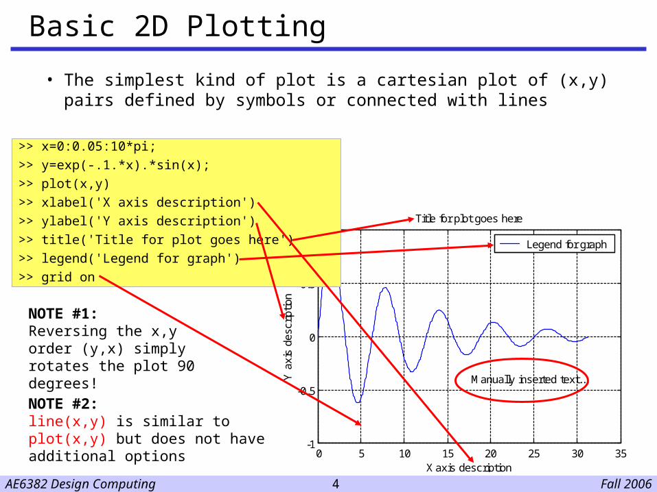
>> x=0:0.05:10*pi;

>> y=exp(-.1.*x).*sin(x);

>> plot(x,y)

>> xlabel('X axis description')

>> ylabel('Y axis description')

>> title('Title for plot goes here')

>> legend('Legend for graph')

>> grid on

Basic 2D Plotting

• The simplest kind of plot is a cartesian plot of (x,y) pairs defined by symbols or connected with lines

NOTE #1:Reversing the x,y order (y,x) simply rotates the plot 90 degrees!

NOTE #2:line(x,y) is similar to plot(x,y) but does not have additional options


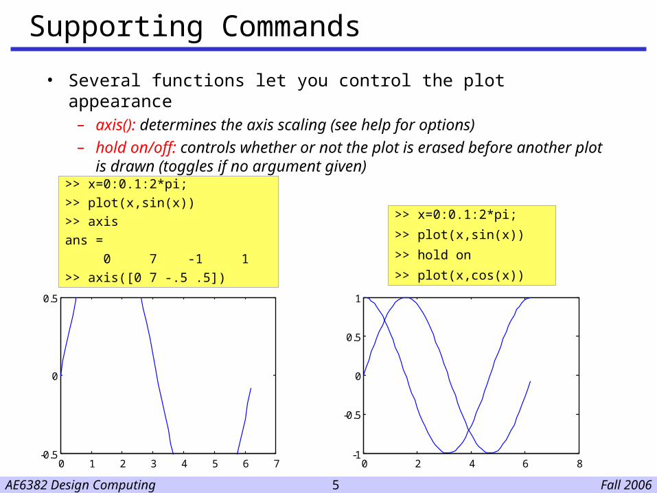
Supporting Commands

• Several functions let you control the plot appearance– axis(): determines the axis scaling (see help for options)– hold on/off: controls whether or not the plot is erased before

another plot is drawn (toggles if no argument given)

>> x=0:0.1:2*pi;

>> plot(x,sin(x))

>> axis

ans =

0 7 -1 1

>> axis([0 7 -.5 .5])

0 1 2 3 4 5 6 7-0.5

0

0.5

>> x=0:0.1:2*pi;

>> plot(x,sin(x))

>> hold on

>> plot(x,cos(x))

0 2 4 6 8-1

-0.5

0

0.5

1


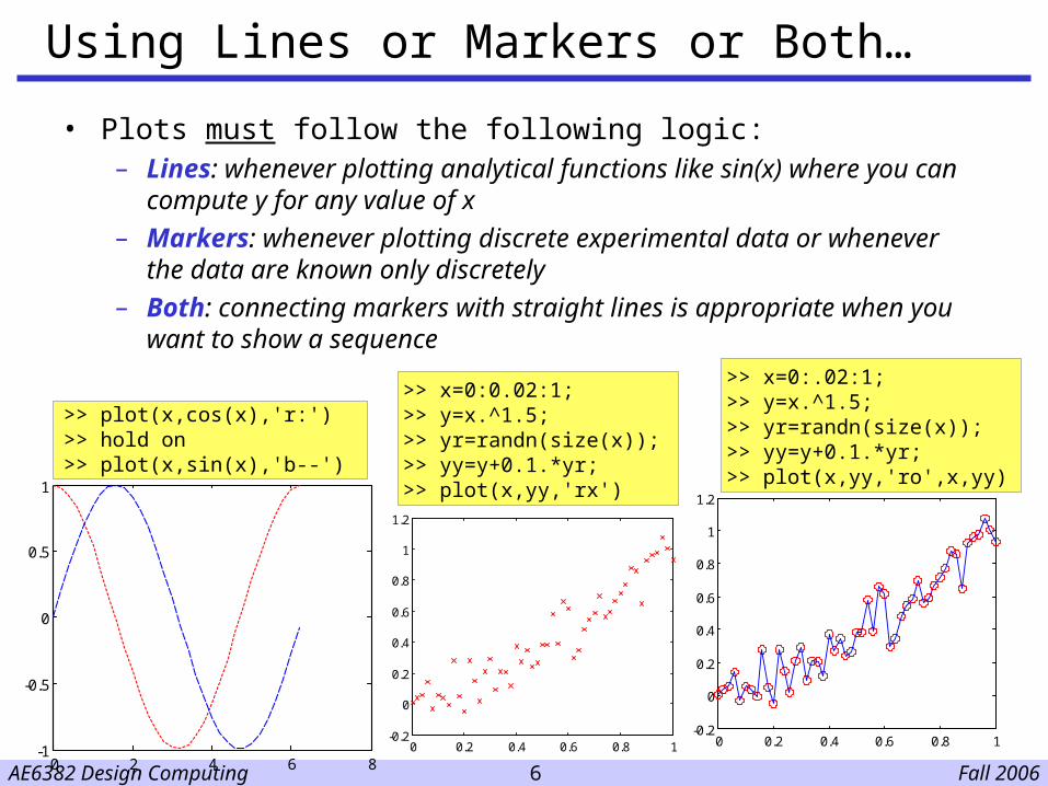
Using Lines or Markers or Both…

• Plots must follow the following logic:– Lines: whenever plotting analytical functions like sin(x) where you can

compute y for any value of x

– Markers: whenever plotting discrete experimental data or whenever the data are known only discretely

– Both: connecting markers with straight lines is appropriate when you want to show a sequence

>> plot(x,cos(x),'r:')>> hold on>> plot(x,sin(x),'b--')

0 2 4 6 8-1

-0.5

0

0.5

1

0 0.2 0.4 0.6 0.8 1-0.2

0

0.2

0.4

0.6

0.8

1

1.2

>> x=0:.02:1;>> y=x.^1.5;>> yr=randn(size(x));>> yy=y+0.1.*yr;>> plot(x,yy,'ro',x,yy)

0 0.2 0.4 0.6 0.8 1-0.2

0

0.2

0.4

0.6

0.8

1

1.2

>> x=0:0.02:1;>> y=x.^1.5;>> yr=randn(size(x));>> yy=y+0.1.*yr;>> plot(x,yy,'rx')


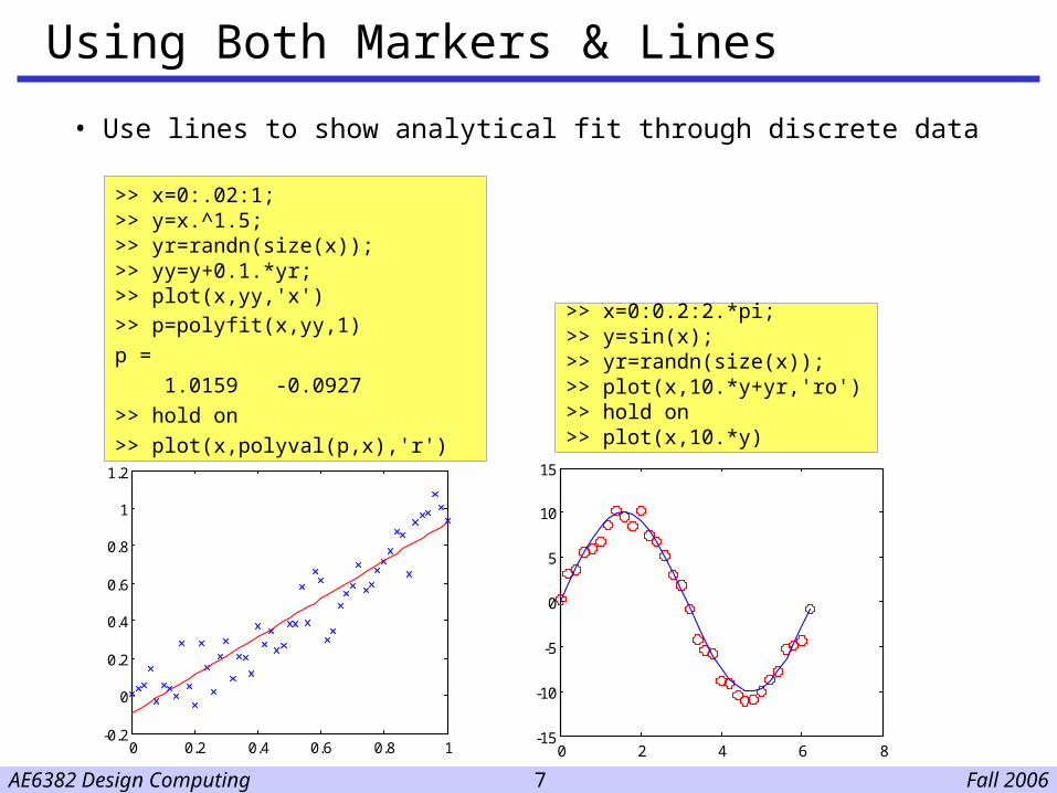
Using Both Markers & Lines

• Use lines to show analytical fit through discrete data

>> x=0:.02:1;>> y=x.^1.5;>> yr=randn(size(x));>> yy=y+0.1.*yr;>> plot(x,yy,'x')

>> p=polyfit(x,yy,1)

p =

1.0159 -0.0927

>> hold on

>> plot(x,polyval(p,x),'r')

0 0.2 0.4 0.6 0.8 1-0.2

0

0.2

0.4

0.6

0.8

1

1.2

0 2 4 6 8-15

-10

-5

0

5

10

15

>> x=0:0.2:2.*pi;>> y=sin(x);>> yr=randn(size(x));>> plot(x,10.*y+yr,'ro')>> hold on>> plot(x,10.*y)


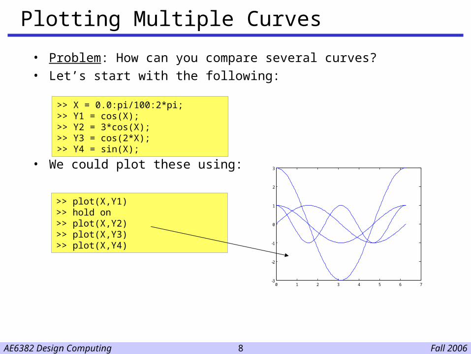
Plotting Multiple Curves

• Problem: How can you compare several curves?• Let’s start with the following:

• We could plot these using:

>> X = 0.0:pi/100:2*pi;>> Y1 = cos(X);>> Y2 = 3*cos(X);>> Y3 = cos(2*X);>> Y4 = sin(X);

>> plot(X,Y1)>> hold on>> plot(X,Y2)>> plot(X,Y3)>> plot(X,Y4)

0 1 2 3 4 5 6 7-3

-2

-1

0

1

2

3


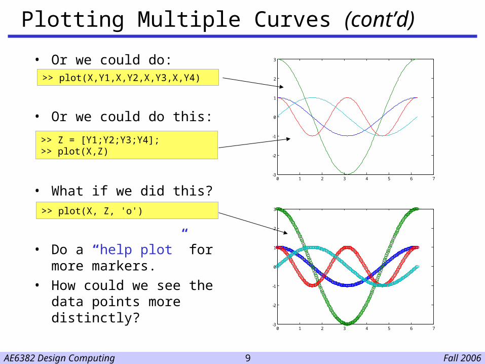
Plotting Multiple Curves (cont’d)

• Or we could do:

• Or we could do this:

• What if we did this?

• Do a “help plot” for more markers.

• How could we see the data points more distinctly?

0 1 2 3 4 5 6 7-3

-2

-1

0

1

2

3

>> plot(X,Y1,X,Y2,X,Y3,X,Y4)

>> Z = [Y1;Y2;Y3;Y4];>> plot(X,Z)

0 1 2 3 4 5 6 7-3

-2

-1

0

1

2

3>> plot(X, Z, 'o')


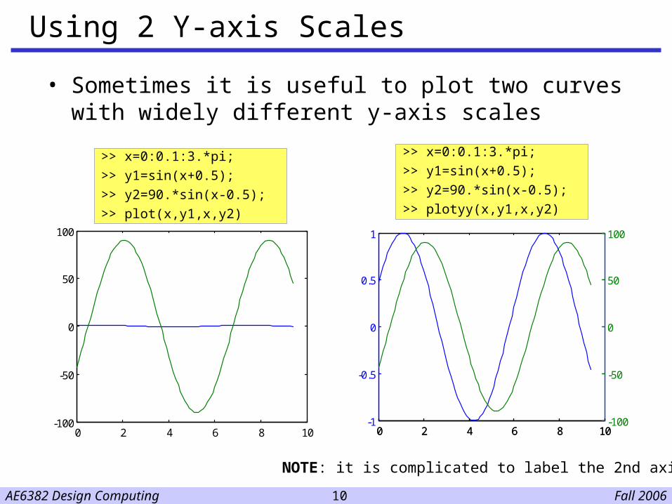
Using 2 Y-axis Scales

• Sometimes it is useful to plot two curves with widely different y-axis scales

>> x=0:0.1:3.*pi;

>> y1=sin(x+0.5);

>> y2=90.*sin(x-0.5);

>> plotyy(x,y1,x,y2)

0 2 4 6 8 10-1

-0.5

0

0.5

1

0 2 4 6 8 10-100

-50

0

50

100

0 2 4 6 8 10-100

-50

0

50

100

>> x=0:0.1:3.*pi;

>> y1=sin(x+0.5);

>> y2=90.*sin(x-0.5);

>> plot(x,y1,x,y2)

NOTE: it is complicated to label the 2nd axis…


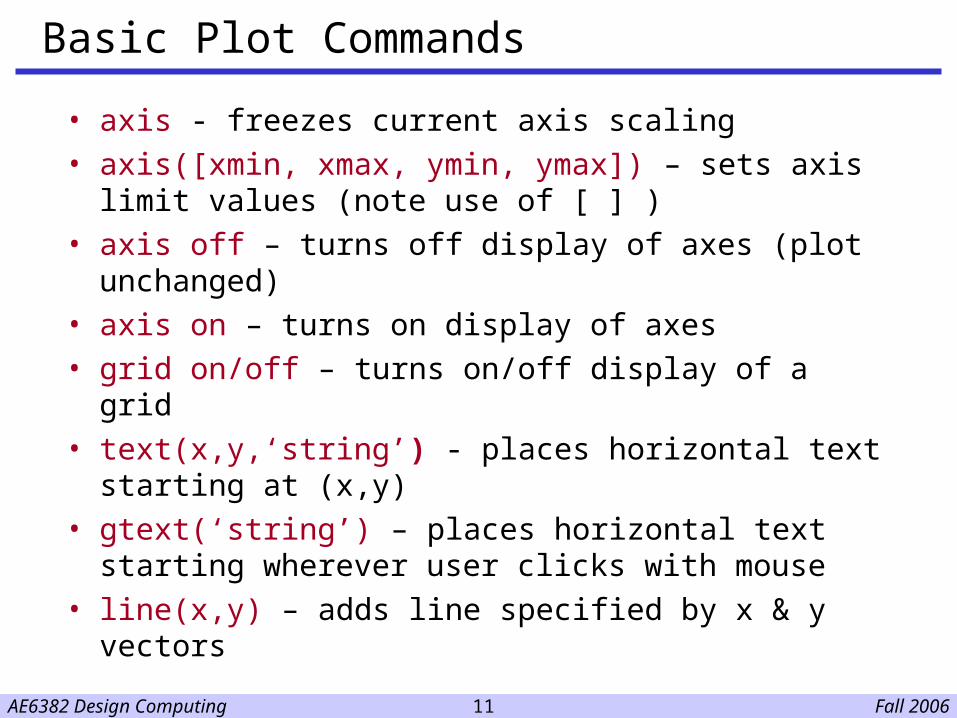
Basic Plot Commands

• axis - freezes current axis scaling• axis([xmin, xmax, ymin, ymax]) – sets axis

limit values (note use of [ ] )• axis off – turns off display of axes (plot unchanged)• axis on – turns on display of axes• grid on/off – turns on/off display of a grid• text(x,y,‘string’) - places horizontal text starting

at (x,y)• gtext(‘string’) – places horizontal text starting

wherever user clicks with mouse• line(x,y) – adds line specified by x & y vectors


Example of Log Plots

• Using a log scale can reveal large dynamic ranges

>> x=linspace(.1,10,1000);

>> damp=0.05;

>> y=1./sqrt((1-x.^2).^2 + (2.*damp.*x).^2);

>> plot(x,y)

>> semilogx(x,y)

>> loglog(x,y)

0 2 4 6 8 100

2

4

6

8

10

10-1

100

101

0

2

4

6

8

10

10-1

100

101

10-2

10-1

100

101

Describes the behavior of vibrating systems

1/ 22 2 2

1

(1 ) (2 )y

x x


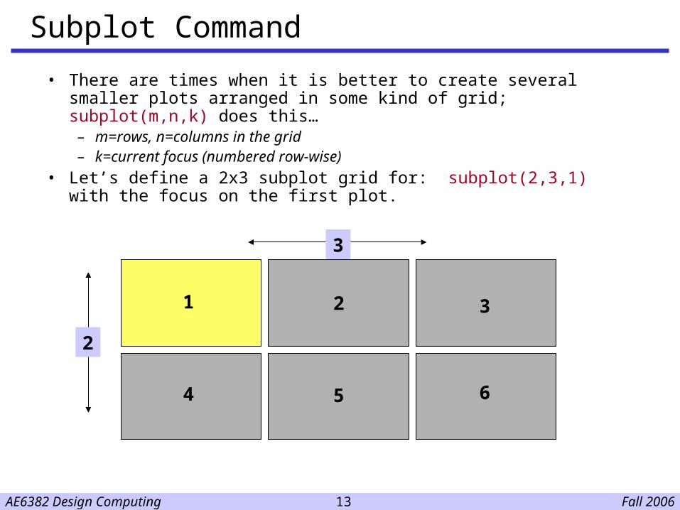
Subplot Command

• There are times when it is better to create several smaller plots arranged in some kind of grid; subplot(m,n,k) does this…– m=rows, n=columns in the grid – k=current focus (numbered row-wise)

• Let’s define a 2x3 subplot grid for: subplot(2,3,1) with the focus on the first plot.

2

3

1 2

5 6

3

4


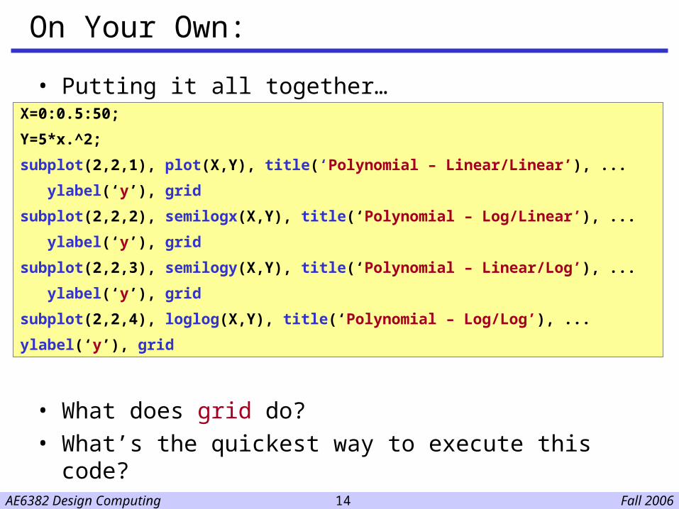
On Your Own:

• Putting it all together…

• What does grid do?• What’s the quickest way to execute this code?

X=0:0.5:50;

Y=5*x.^2;

subplot(2,2,1), plot(X,Y), title(‘Polynomial – Linear/Linear’), ...

ylabel(‘y’), grid

subplot(2,2,2), semilogx(X,Y), title(‘Polynomial – Log/Linear’), ...


subplot(2,2,3), semilogy(X,Y), title(‘Polynomial – Linear/Log’), ...


subplot(2,2,4), loglog(X,Y), title(‘Polynomial – Log/Log’), ...



Specialized 2D Plots

• There are a number of other specialized 2D plots– area(x,y): builds a stacked area plot– pie(): creates a pie chart (with options)– bar(x,y): creates a vertical bar chart (with many options)– stairs(x,y): similar to bar() but shows only outline– errorbar(x,y,e): plots x vs y with error bars defined by e– scatter(x,y): creates a scatter plot with options for markers– semilogx(x,y): plots x vs y with x using a log scaling– semilogy(x,y): plots x vs y with y using a log scaling– loglog(x,y): plots x vs y using log scale for both axes

– And many others… (explore these yourself; you may find a good use in a later course)

– Chapter 25 in Mastering Matlab is a good starting point.


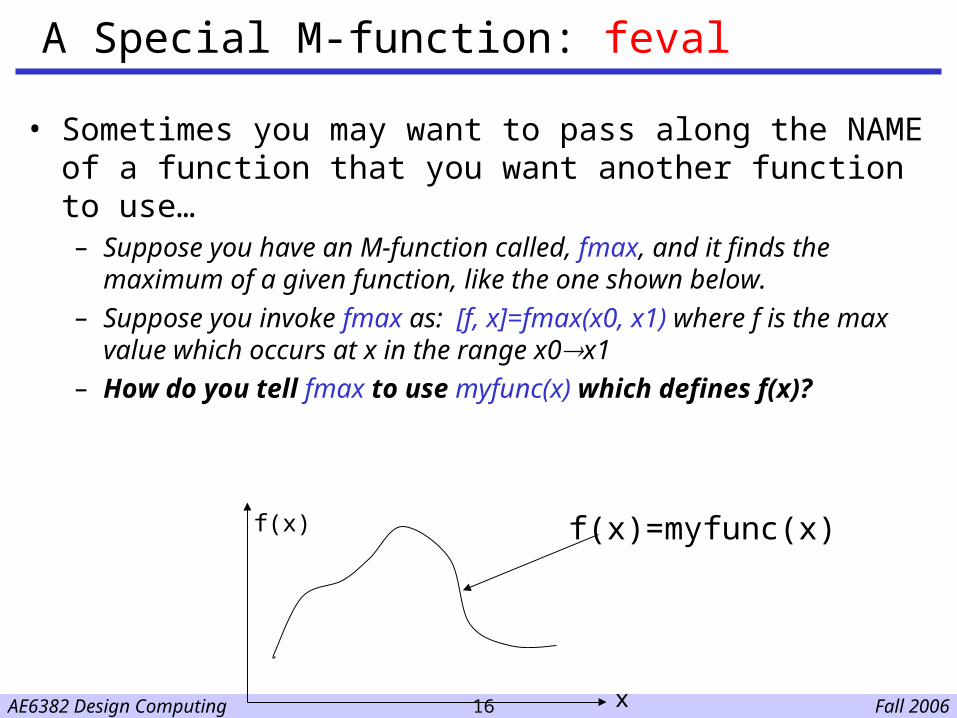
A Special M-function: feval

• Sometimes you may want to pass along the NAME of a function that you want another function to use…– Suppose you have an M-function called, fmax, and it finds the

maximum of a given function, like the one shown below.– Suppose you invoke fmax as: [f, x]=fmax(x0, x1) where f is

the max value which occurs at x in the range x0x1– How do you tell fmax to use myfunc(x) which defines f(x)?

f(x)

x

f(x)=myfunc(x)


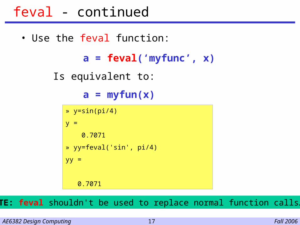
feval - continued

• Use the feval function:

a = feval(‘myfunc’, x)

Is equivalent to:

a = myfun(x)

» y=sin(pi/4)

y =

0.7071

» yy=feval('sin', pi/4)

yy =

0.7071

NOTE: feval shouldn't be used to replace normal function calls…


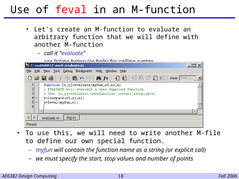
Use of feval in an M-function

• Let's create an M-function to evaluate an arbitrary function that we will define with another M-function– call it "evaluate"

– see listing below (or help) for calling syntax

• To use this, we will need to write another M-file to define our own special function.– myfun will contain the function name as a string (or explicit call)

– we must specify the start, stop values and number of points


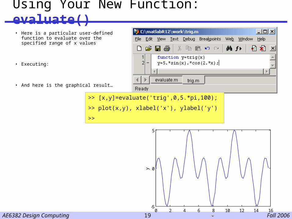
Using Your New Function: evaluate()

• Here is a particular user-defined function to evaluate over the specified range of x values

• Executing:

• And here is the graphical result…

0 2 4 6 8 10 12 14 16-5

0

5

x

y

>> [x,y]=evaluate('trig',0,5.*pi,100);

>> plot(x,y), xlabel('x'), ylabel('y')

>>


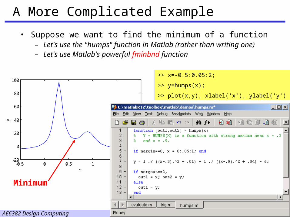
A More Complicated Example

• Suppose we want to find the minimum of a function– Let's use the "humps" function in Matlab (rather than writing one)– Let's use Matlab's powerful fminbnd function

-0.5 0 0.5 1 1.5 2-20

0

20

40

60

80

100

x

y

>> x=-0.5:0.05:2;

>> y=humps(x);


Minimum


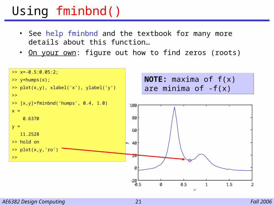
Using fminbnd()

• See help fminbnd and the textbook for many more details about this function…

• On your own: figure out how to find zeros (roots)

-0.5 0 0.5 1 1.5 2-20

0

20

40

60

80

100

x

y

>> x=-0.5:0.05:2;

>> y=humps(x);


>>

>> [x,y]=fminbnd('humps', 0.4, 1.0)

x =

0.6370

y =

11.2528

>> hold on

>> plot(x,y,'ro')

>>

NOTE: maxima of f(x) are minima of -f(x)NOTE: maxima of f(x) are minima of -f(x)


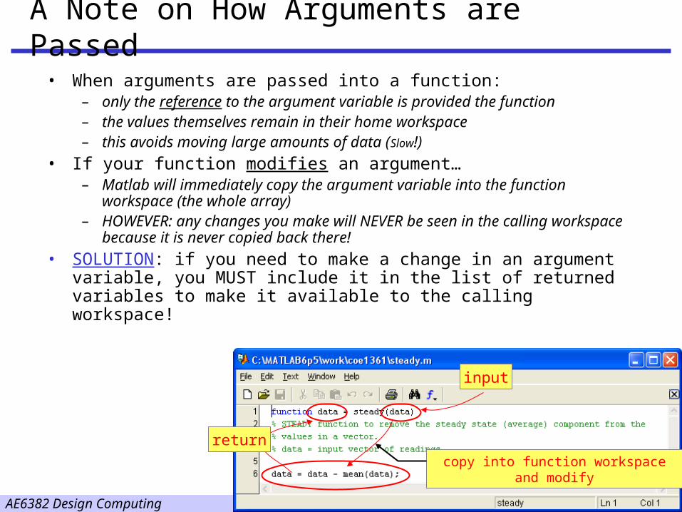
A Note on How Arguments are Passed

• When arguments are passed into a function:– only the reference to the argument variable is provided the function– the values themselves remain in their home workspace– this avoids moving large amounts of data (Slow!)

• If your function modifies an argument…– Matlab will immediately copy the argument variable into the function

workspace (the whole array)– HOWEVER: any changes you make will NEVER be seen in the calling

workspace because it is never copied back there!

• SOLUTION: if you need to make a change in an argument variable, you MUST include it in the list of returned variables to make it available to the calling workspace!

input

copy into function workspace and modify

return


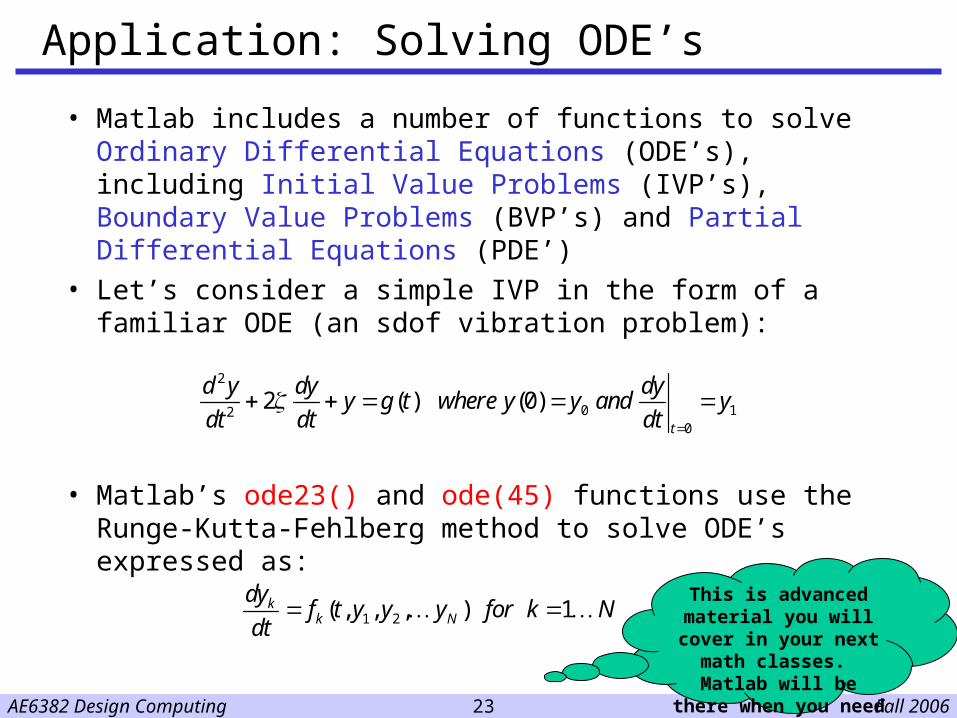
Application: Solving ODE’s

• Matlab includes a number of functions to solve Ordinary Differential Equations (ODE’s), including Initial Value Problems (IVP’s), Boundary Value Problems (BVP’s) and Partial Differential Equations (PDE’)

• Let’s consider a simple IVP in the form of a familiar ODE (an sdof vibration problem):

• Matlab’s ode23() and ode(45) functions use the Runge-Kutta-Fehlberg method to solve ODE’s expressed as:

2

0 120

2 ( ) (0)t

d y dy dyy g t where y y and y

dt dt dt

1 2( , , , ) 1kk N

dyf t y y y for k N

dt

This is advanced material you will cover

in your next math classes. Matlab will be there when you need it!


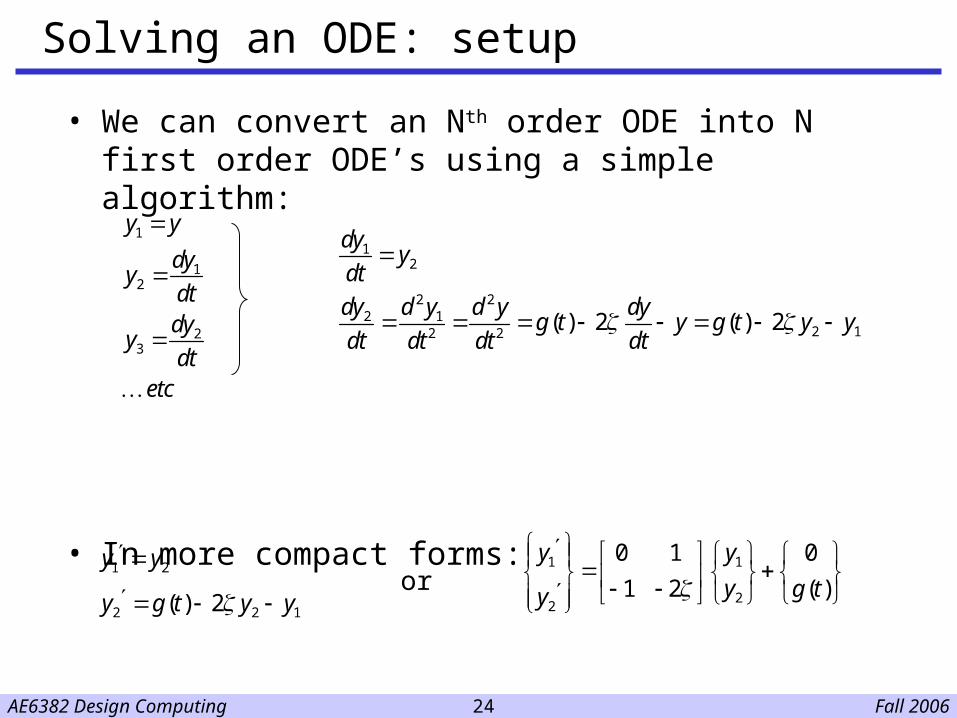
Solving an ODE: setup

• We can convert an Nth order ODE into N first order ODE’s using a simple algorithm:

• In more compact forms:

1

12

23

y y

dyy

dtdy

ydt

etc

12

2 22 1

2 12 2( ) 2 ( ) 2

dyy

dt

dy d y d y dyg t y g t y y

dt dt dt dt

1 2

2 2 1( ) 2

y y

y g t y y

1 1

22

0 1 0

1 2 ( )

y y

y g ty

or


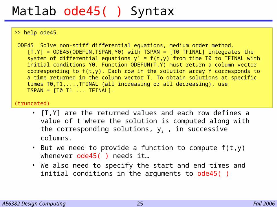
Matlab ode45( ) Syntax

• [T,Y] are the returned values and each row defines a value of t where the solution is computed along with the corresponding solutions, yi , in successive columns.

• But we need to provide a function to compute f(t,y) whenever ode45( ) needs it…

• We also need to specify the start and end times and initial conditions in the arguments to ode45( )

>> help ode45

ODE45 Solve non-stiff differential equations, medium order method. [T,Y] = ODE45(ODEFUN,TSPAN,Y0) with TSPAN = [T0 TFINAL] integrates the system of differential equations y' = f(t,y) from time T0 to TFINAL with initial conditions Y0. Function ODEFUN(T,Y) must return a column vector corresponding to f(t,y). Each row in the solution array Y corresponds to a time returned in the column vector T. To obtain solutions at specific times T0,T1,...,TFINAL (all increasing or all decreasing), use TSPAN = [T0 T1 ... TFINAL].

(truncated)


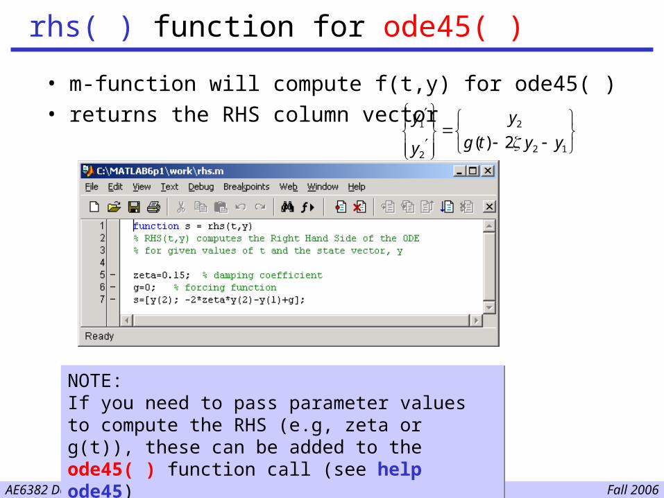
rhs( ) function for ode45( )

• m-function will compute f(t,y) for ode45( )• returns the RHS column vector 1 2

2 12

( ) 2

y y

g t y yy

NOTE:If you need to pass parameter values to compute the RHS (e.g, zeta or g(t)), these can be added to the ode45( ) function call (see help ode45)

NOTE:If you need to pass parameter values to compute the RHS (e.g, zeta or g(t)), these can be added to the ode45( ) function call (see help ode45)


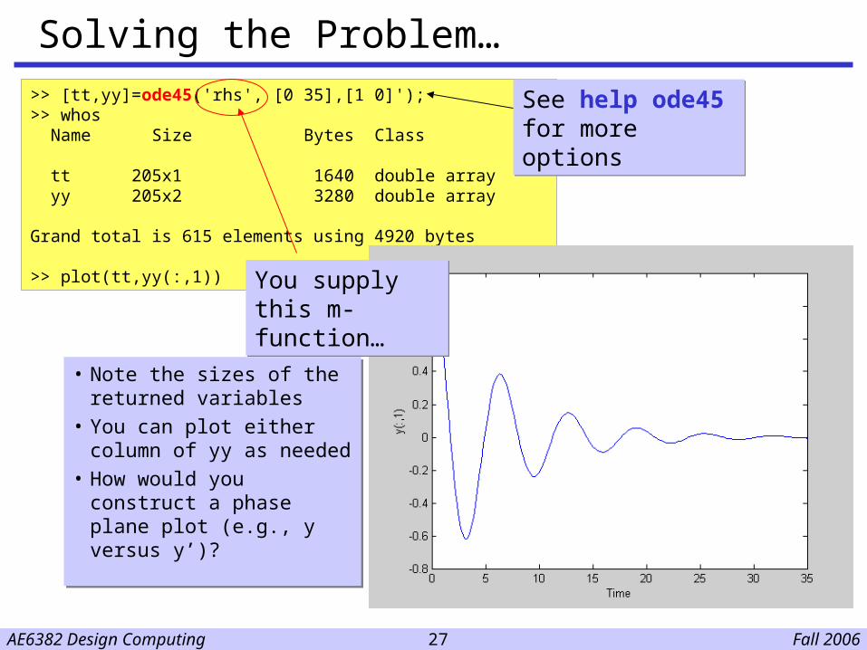
Solving the Problem…

• Note the sizes of the returned variables

• You can plot either column of yy as needed

• How would you construct a phase plane plot (e.g., y versus y’)?

• Note the sizes of the returned variables

• You can plot either column of yy as needed

• How would you construct a phase plane plot (e.g., y versus y’)?

>> [tt,yy]=ode45('rhs', [0 35],[1 0]');>> whos Name Size Bytes Class

tt 205x1 1640 double array yy 205x2 3280 double array

Grand total is 615 elements using 4920 bytes

>> plot(tt,yy(:,1))

See help ode45 for more optionsSee help ode45 for more options

You supply this m-function…You supply this m-function…


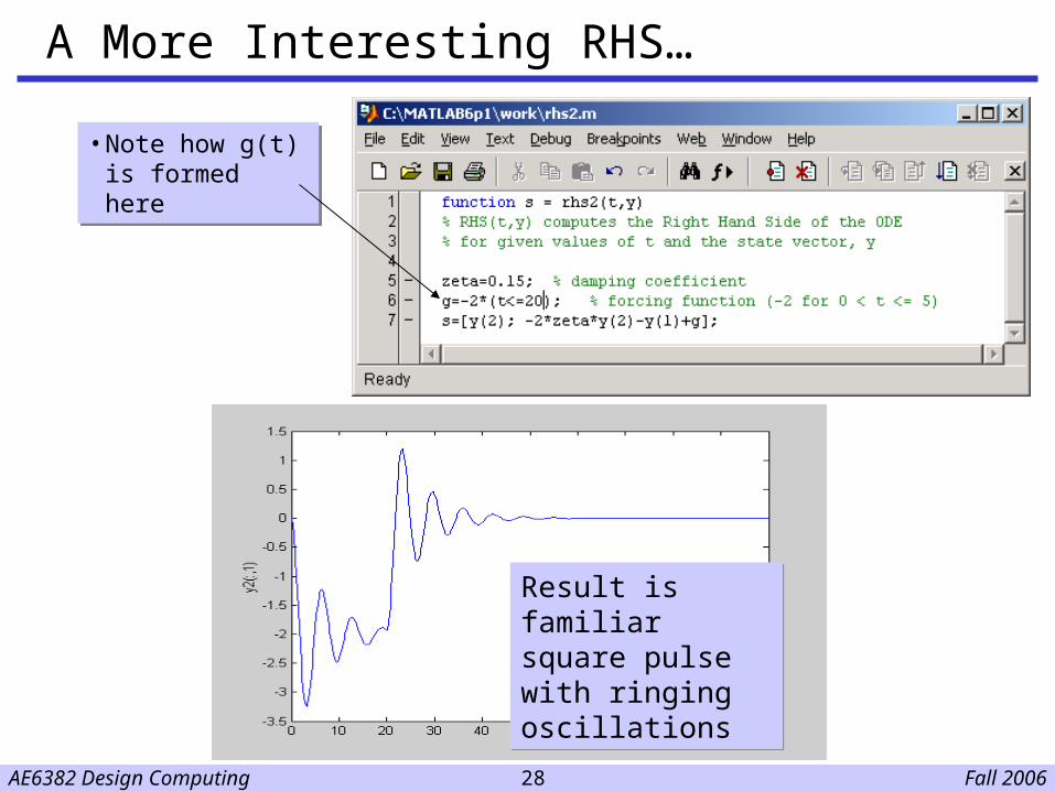
A More Interesting RHS…

• Note how g(t) is formed here

• Note how g(t) is formed here

Result is familiar square pulse with ringing oscillations

Result is familiar square pulse with ringing oscillations


Summary

• Review questions– Describe 2D plotting in MATLAB,– What is a figure? What is an axis?– How do you create a plot of two curves? More than 2 curves?– What is a legend and how is it created?– What kinds of 2D plots are available?

• Action Items

– Review the lecture and run all demos

– Look over the help for the plot, axis, label and figure m-functions

– Try constructing a polar plot

fall 2006ae6382 design computing1 2d plotting in matlab learning objectives discover how matlab can...

Documents

y order y

yr plotx

sinx plotx

cartesian plot of x

pi plotx

randnsizex plotx

y pairs

sequence plotx