Fama-French in China:Size and Value Factors in Chinese Stock Returns

Can Chen, Xing Hu, Yuan Shao and Jiang Wang∗

February 8, 2015

Abstract

We investigate the size and value factors in the cross-section of returns for the Chinese

stock market. We find a significant size effect but no robust value effect. A zero-

cost small-minus-big (SMB) portfolio earns an average premium of 0.85% per month,

which is statistically significant with t-value of 3.09 and important economically. In

contrast, neither the market portfolio nor the zero-cost high-minus-low (HML) portfolio

has average premiums statistically different from zero. In both time-series regressions

and Fama-Macbeth cross-sectional tests, SMB appears to be the strongest factor in

explaining the cross-section of Chinese stock returns. Our results contradict most of the

existing literature which finds a significant value effect. We show that this difference

comes from the extreme values in a few months in the early years of the market (1995

to 1996), which turn out to have a heavy impact on the average premiums given the

relatively short history of the Chinese stock market.

∗Chen and Shao are from Shanghai Jiao Tong University (cchen.10@saif.sjtu.edu.cn andyshao.10@saif.sjtu.edu.cn, respectively), Hu is from University of Hong Kong and CAFR (gracehu@hku.edu,corresponding author), and Jiang Wang is from MIT Sloan School of Management, CAFR and NBER(wangj@mit.edu). The authors acknowledge the support from China Academy of Financial Research (CAFR)and are grateful to Chenjun Fang, Yue Hu and Lun Li for valuable research assistance. The authors alsobenefited greatly from comments from Jun Pan.

1 Introduction

A large body of asset pricing literature has been devoted to document and explain cross-

sectional stock returns beyond the classic Capital Asset Pricing Model (CAPM). Earlier papers

include Stattman (1980), Banz (1981), Basu (1983) and Chan, Hamao, and Lakonishok (1991),

which found empirical cross-sectional return patterns inconsistent with the CAPM. In two

influential papers, Fama and French (1992) and Fama and French (1993), the authors examined

various factors and showed that size, as measured by market capitalization, and value, as

measured the book-to-market ratio, are the two most significant factors in explaining the

cross-sectional returns in the U.S. stock market. Since then, size and value premiums have

become two of the most-widely used “asset-pricing” factors in the U.S. and global equity

markets.1

There has been very limited study on the cross-sectional returns in the Chinese stock

market, even though it has quickly grown to be the second largest in the world by market

capitalization (see, for example, monthly report for 2014 by the World Federation of Ex-

changes). Research has been hindered by the lack of high quality data and by the short

history of the market. Existing work rely on data of varied quality and sample periods and

obtain results often inconsistent with each other.2 Such a situation is particularly unsatisfying

as most empirical work on the market needs an empirical pricing model to benchmark risk and

returns. Taking advantage of a complete database recently put together, we hope to provide

a more definitive empirical calibration of the return factors in the Chinese stock market.

In particular, we examine the role of size and value factors in explaining the cross-sectional

returns in the Chinese A-share market from its beginning in 1990 to 2013. Our benchmark

sample period is from July 1997 to December 2013, when there is enough number of stocks

in the cross-section, although our main conclusions remain the same when earlier years were

1Studies of non-US markets include Fama and French (2012), Bruckner, Lehmann, Schmidt, and Stehle(2014), Michou, Mouselli, and Stark (2013), Veltri and Silvestri (2011), Moerman (2005), Nartea, Gan, andWu (2008), Chou, Ko, Kuo, and Lin (2012), Docherty, Chan, and Easton (2013), Cordeiro and Machado(2013), Agarwalla, Jacob, and Varma (2013), Drew and Veeraraghavan (2002), among others.

2See, for example, Nusret Cakici and Topyan (2011), Carpenter, Lu, and Whitelaw (2014), Chen, Kim,Yao, and Yu (2010), and Wang and Xu (2004), among others. We will discuss these papers in more detaillater.

1

included. We find that size is strongly associated with cross-sectional returns. The average

returns on the 10 portfolios formed on the basis of market capitalization show a robust negative

relationship with underlying stocks’ size. The average returns on the smallest size decile is

2.05% per month during the period, versus 0.42% on the largest size decile. The difference

in average returns is 1.63% per month, not only economically large but also strongly positive

significant at the 1% level. Moreover, the observed relationship between stock returns and

firm size cannot be explained by the market factor, as the market βs are flat across the ten

size-sorted portfolios. In contrast, the average returns on 10 portfolios formed on the basis of

book-to-market ratios do not exhibit any clear pattern, suggesting that the value factor is not

associated with cross-sectional stock returns.

We then follow the methodology in Fama and French (1993) to construct two zero-cost

portfolios, SMB and HML, to mimic risk factors related to size and value in the Chinese stock

market. Over the period from July 1997 to December 2013, SMB earns an average return of

0.85% per month, or 10.2% per year. The average return of SMB is not only economically

large but also strongly positive significant with t-value 3.09. In contrast, neither the market

portfolio RM − Rf nor the factor mimicking portfolio HML has significant average returns

during the same sample period. The average excess return of the market portfolio is 0.60%

per month with t-value 0.97; the average return of HML is 0.34% per month with t-value 1.61.

The dominant performance of SMB over the market portfolio and HML implies that size is

likely to be important in explaining cross-sectional returns, while the market portfolio and

HML are not.

For formal asset pricing tests, we employ both the time-series and the Fama-Macbeth

regressions approaches. In the time-series regressions, we first form 25 portfolios on the basis

of size and book-to-market ratio. There is a large dispersion in average excess returns across

the 25 portfolios, ranging from 0.11% per month to 1.91% per month. Among them, eight

portfolios have significant positive average excess returns. We then regress the excess returns

of 25 stock portfolios on the market portfolio RM−Rf and the two factor mimicking portfolios

SMB and HML.

The time-series regressions results show that the three factors capture strong common

variations in stock returns of the 25 portfolios, as reflected in the significant slopes on the

2

three risk factors and the high R2 values of the regressions. More important, judging on the

basis of the intercepts of the time-series regressions, the three factors together successfully

capture the cross-sectional variations in average returns on the 25 portfolios. The remaining

intercepts, αs, of the regressions of the excess returns on the 25 portfolios on the three factors,

RM −Rf , SMB and HML, are small in magnitude, ranging from -0.28% to 0.26% per month,

and are not significantly different from zero. The Gibbons-Ross-Shanken F-statistic is 0.93

with probability 0.435, therefore we can’t reject the hypothesis that the intercepts across the

25 portfolios are jointly zero.

Moreover, the three factors contribute differently to the reduction of αs. Using the market

factor alone, the intercepts are decreased relative to the excess returns, but remain strongly

significant and widely dispersed. Ten out of the 25 portfolios still have positive significant

αs and one portfolio has negative significant α. In contrast, SMB, when used as the sole

risk factor, makes all intercepts in the time-series regressions not statistically significantly

different from zero. However, 24 out of the 25 αs remain positive and large. The highest α

is at 0.74% per month. Adding the market factor with SMB can further reduce the size of

αs to be within a range from -0.42% to 0.31%. Among the 25 portfolios, only one portfolio’s

excess returns is over-corrected with negative α of -0.41% and t-value of -1.99. In contrast to

the strong explanatory power of SMB, HML plays a weak role in explaining cross-sectional

returns. Whether used alone or in combination with the market factor, the intercepts for most

portfolios in the bottom two size quintiles remain large and statistically significant. Putting

all evidence together, it is clear that SMB is the most important factor in explaining the

cross-sectional variations in average stock returns.

We also perform Fama-Macbeth regressions to estimate the risk-premiums associated with

the market, SMB and HML factors. The results are consistent with the time-series regression

findings. SMB is estimated to have a risk premium of 0.98% per month, strongly positively

significant with t-value of 3.22. The positive risk premium associated with SMB is also robust

to the inclusion of various accounting variables. In addition, the magnitude of the size premium

estimated from the Fama-Macbeth regressions is close to the time-series average of the SMB

factor, which is at 0.85% per month with standard error 0.28% per month. The Fama-Macbeth

regressions also confirm that the market factor and HML don’t carry significant risk premiums,

3

again, consistent with the observation that the time-series averages of the market and HML

factors are not statistically significant from zero.

Thus, we find a strong size effect and no value effect cross returns in China’s stock market.

These results, although consistent with Wang and Xu (2004), which is based on a much

shorter sample period from 1996 to 2002, contradict with most of the existing literature on

the Chinese stock market. For example, Chen, Kim, Yao, and Yu (2010), Nusret Cakici and

Topyan (2011) and Carpenter, Lu, and Whitelaw (2014) all document strong size and value

effect. We find that the disagreement stems mainly from different choices of sample periods.

Our sample period starts from July 1997, while other papers usually include an earlier period

from 1995 to 1996.

To reconcile the differences, we test the robustness of our results by expanding our sample

period to start from July 1995 and end at December 2013, covering a total of 222 months. The

size effect remains robust. However, the significant value effect documented in the previous

literature is very fragile and largely driven by extreme estimates in several months during

the early period. The estimated slopes on the HML betas are extremely noisy before July

1997. For examples, the estimated slope is 42.12% on October 1996 and 38.35% on July

1996, much higher than the average level of 0.65% per month, especially when considering

the time-series standard deviation is a mere 4.83% from July 1995 to December 2013. If our

sample were large enough, a few outliers are harmless. However, due to the short-history of

the Chinese stock market, the outliers in the earlier period turn out to have a heavy impact

on the estimated average premiums and the associated t-values. In fact, once we weight

the monthly premium slopes by the number of stocks in the Fama-Macbeth regressions or

remove two extreme months, July 1996 and October 1996, the premium of HML is no-longer

statistically significant. By comparison, the risk premium of size survives all robustness tests.

As a result, we conclude that the previous documented value effect in the Chinese market is

not robust.

The rest of paper is organized as follows. Section 2 gives a short summary of China’s

stock market. Section 3 describes the data we use for this paper. Section 4 discusses the

cross-sectional returns related to size and book-to-market ratio. Section 5 performs formal

asset-pricing tests on the two factor mimicking portfolios SMB and HML. Section 6 conducts

4

several robustness checks. Section 7 concludes the paper.

2 Background on China’s Stock Market

The contemporary Chinese stock market is marked by the founding of two major stock ex-

changes, the Shanghai Stock Exchange (SSE) and the Shenzhen Stock Exchange (SSE), in

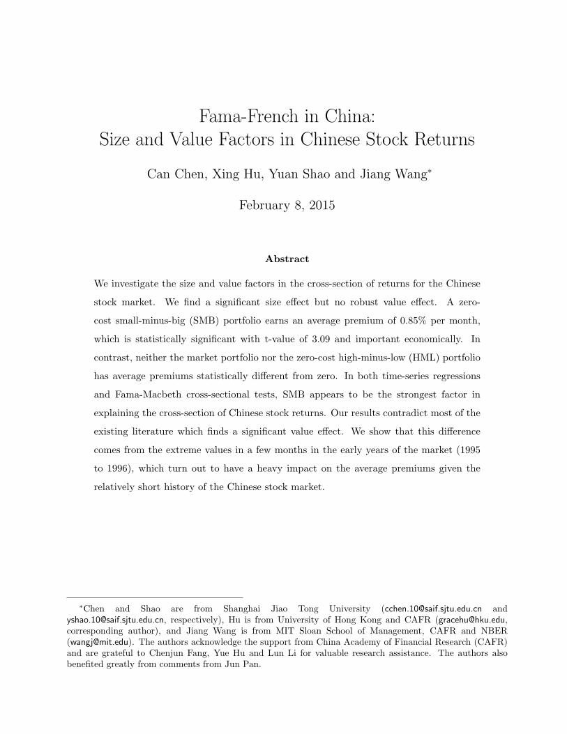
1990. Despite its short history, China’s stock market has experienced a rapid growth. Figure 1

shows the number of stocks and total market capitalization of the Shanghai and Shenzhen ex-

changes from 1990 to 2013. We only mention some relevant facts here. A more comprehensive

summary of the history of China’s stock market and its empirical properties can be found in

Wang, Hu, and Pan (2014).

Starting with only eight stocks listed on Shanghai and six listed on Shenzhen, the number

of stocks on the two exchanges rose to 311 by the end of 1995, 720 by 1997, 1,060 by 2000

and 2,349 by 2013. The two exchanges shared similar growth path in terms of the number of

stocks until 2004, when the Shenzhen exchange expanded more quickly with the creation of

the Small and Medium Enterprise (SME) board. The introduction of the Growth Enterprise

Market (SEM) later at 2009 also substantially increased the number of stocks on the Shenzhen

exchange. By the end of 2013, the number of stocks listed on the Shenzhen Stock Exchange has

reached 1,438, 58% more than that on the Shanghai Exchange. Though with multiple boards

and significantly more stocks, the total market capitalization of the Shenzhen exchange is still

less than that of Shanghai since firms listed on the Shenzhen exchange are usually smaller

companies. Combined the two exchanges together, the total market capitalization reached

37.2 trillion RMB (6 trillion USD) by the end of 2014, putting China in second place globally,

only after the United States (from the World Federation of Exchanges monthly report of Dec

2014).

The Chinese stock market is marked by a number of unique characteristics. One feature

is the co-existence of different share classes. There are three different types of shares in

China’s stock market: A, B and H shares. A shares are dominated in renminbi (RMB)

and are open mostly to domestic investors. B shares, usually dominated in U.S. dollars on

the Shanghai Stock Exchange and Hong Kong dollars on the Shenzhen Stock Exchange, are

5

(a) Number of Listed Firms (b) Total Stock Market Capitalization

Figure 1: Growth of the Shanghai and Shenzhen Stock Exchanges from 1990 to 2013.

mainly for foreign investors. Domestic investors are restricted from investing abroad and

foreign investors are also restricted from investing in the A-share market in mainland China.

However, the issuance and trading activities in the B shares market have decreased sharply

recently, due to various programs that relax the cross-trading restrictions. By the end of

2013, there are only 104 listed companies with B shares traded on the Shanghai and Shenzhen

exchanges, accounting for only a tiny proportion of the total market. H shares, dominated

in Hong Kong dollars, refer to shares of companies registered in mainland China but listed

and traded on the Hong Kong Stock Exchange. Several empirical studies, such as Chan,

Menkveld, and Yang (2008), Mei, Scheinkman, and Xiong (2009), have shown that there are

often substantial price discrepancies between B and H shares and their A-share counterparts

issued by the same company.

Even for just A-shares, many listed Chinese firms have two different types of shares,

“floating” and “non-floating” shares, often referred as the “split-share structure.” Floating

shares are shares issued to the public, which are listed and traded on exchanges and can be

invested by domestic individuals and institutions. They are regarded as different from the

pre-existing “non-floating” shares that often belong to different parts of government. The

latter are often traded via negotiations between various government and semi-government

entities and later other legal entities, typically at book value. Through various reforms aimed

at reducing state-ownership in most state-owned enterprises and shifting them toward a more

market driven environment, non-floating shares are gradually converted into floating shares.

6

By the end of 2013, the proportion of the market capitalization of non-floating shares dropped

to 16.5% from the peak of near 90% in early 1990. In this paper, we will mainly focus on

floating A shares, which represent what domestic investors can trade publicly in China’s stock

market.

The Shanghai and Shenzhen stock exchanges have a similar trading mechanism, in which

orders are executed through a centralized electronic limit order book, based on the principle

of price and time priority. Both exchanges impose daily price limits on traded stocks. The

policy on price limits has gone through several different stages. When the two exchanges were

established in 1990, there were very strict rules on transaction prices and volumes. In the

first few years, trading was quite thin on both exchanges. To encourage trading and improve

market liquidity, the regulators withdrew price limits and adopted a free trading policy on

May 12, 1992. Four years later on December 16, 1996, the government re-introduced the price

limits policy amid concerns over speculation, an overheated market and social stability. The

price limits were set at ±10% of the previous closing price, and has remained unchanged.

Unlike many open international stock markets, there are strict regulations on who can

invest directly in China’s domestic stock market. Major investors can be classified into four

major classes: domestic individuals, domestic institutions, financial intermediaries and finan-

cial service providers (including brokers, integrated securities companies, investment banks

and trust companies) and qualified foreign institutional investors (QFII). It is worth empha-

sizing that, commercial banks in mainland China are forbidden by law from participating

in security underwriting or investing business, except for QFIIs. Commercial banks are also

forbidden from lending funds to their clients for security business. Insurance companies are

permitted to invest in common stocks only indirectly, through asset management products

operated by mutual funds.

3 Data

The data for our study are from the Chinese Capital Market (CCM) Database provided by the

China Academy of Financial Research (CAFR). The CCM database covers basic accounting

data and historical A-share returns for all Chinese stocks listed on the Shanghai and Shenzhen

7

exchanges from 1991 to 2013.3

Although the Chinese stock market began in 1990, our main results are based on a sample

from 1997 to 2013. There are a number of considerations for this choice. The first is that the

number of stocks available in the early period was too limited to conduct any meaningful cross-

section tests. There were very few stocks traded on the Shanghai and Shenzhen exchanges in

their early days - eight stocks were listed in Shanghai in 1990 and six were listed in Shenzhen

in 1991. It was until late 1996 when the number of stocks listed on the two exchanges first

crossed the 500 benchmark. In addition, the stock market was extremely volatile in the early

1990s. For example, realized volatility measured over a one-month horizon was above 60% on

May 1995 and December 1996. Since 1997, the stock market has became more stable. Market

volatility moves around 20% most of the time, except during the 2007-2008 financial crisis.

The last consideration is regulation changes, especially the price limits policy. The current

10% price limits were imposed on December 16, 1996. Before that, the price limit policy was

changed for several times. Balancing these factors and the desire to have a sample as long

as possible, we decide to use the sample from 1997 to 2013 for our main analysis. Though it

covers a shorter period, our sample has a rich number of cross-sectional firms during a period

with a relatively stable market and regulatory environment. In the robustness check section,

we test the robustness of our main results by expanding the sample to include two earlier

years, 1995 and 1996. Our main results stay the same by including these two years.

We match the accounting data for all Chinese firms in calendar year t−1 (1996 - 2012) with

the returns from July of year t to June of t+1. The accounting data is extracted from annual

reports filed by companies listed on the Shanghai and Shenzhen stock exchanges. Because

all public Chinese firms end their fiscal year in December and are required by law to submit

their annual reports no later than the end of April, the six-month lag between accounting

data and returns ensures that accounting variables are publicly available and the embedded

information has been properly reflected in market prices. This match is also consistent with

the standard approaches used in the literature for the U.S. market.

Our main accounting variables are size and book-to-market equity ratio. A firm’s size is

3For details on the CCM database, readers can refer to Wang, Hu, and Pan (2014) and the data manualpublished by CAFR.

8

measured as the floating A-share market capitalization at the end of June each year. We

use only floating A shares to compute the size of a listed company for two reasons. First,

only floating A shares are investable for general domestic investors, while non-floating shares

or other types of floating shares such as B and H are not. Second, non-floating shares are

not actively traded and their transaction prices are not determined in the open market but

through private negotiations. Therefore, floating A-share is the only share class that can be

invested by a general domestic investor and has precise market prices. We think it is the most

proper variable for measuring the size of a listed company. There are, of course, many other

ways to construct the size variable. In the robustness check section, we confirm that our main

results are robust to different size measures.

Following the same spirit, we calculate the book-to-market ratio (B/M) as the fraction

of book value of equity per share and floating A-share prices at the end of December in the

previous year t − 1. The numerator is the total book value divided by the total number of

shares, which include A-, B-, H- share classes and both floating and non-floating shares. This

adjustment ensures that the numerator for the B/M ratio calculation represents the book

value for one unit of floating A-share. Other accounting variables include A/ME, A/BE, E/P

and D/P ratios. A/ME is market leverage, measured as asset per share divided by floating

A-share price at the end of December of year t − 1; A/BE is book leverage, measured as

asset per share divided by book value of equity per share. E(+)/P is total positive earnings

divided by price; E/P dummy is a dummy variable which takes zero if earning is positive and

one otherwise. The price P in the denominators for the above ratios is the floating A-share

price at the end of December in the previous year t-1. D/P is the ratio between all dividends

distributed in the one year horizon before the end of June and the floating A-share price at

the end of June.

4 Cross-sectional returns in China’s Stock Market

4.1 Univariate Sorted Portfolios

To investigate potential size and value effect in cross-sectional returns of Chinese listed firms,

we first look at performances of 10 size- and B/M-sorted portfolios. At the end of June of each

9

year from 1997 to 2012, we divide all non-financial firms listed on the Shanghai and Shenzhen

exchanges into 10 equally populated groups on the basis of their size or B/M ratios. The

portfolios are kept unchanged for the following twelve months, from July to June next year.

returns for the 10 portfolios are calculated as the equal-weighted average of individual stock

returns.

Table 1 reports the average excess returns and firm characteristics of the 10 univariate

sorted portfolios, panel A for the size-sorted portfolios and panel B for the B/M-sorted port-

folios. When portfolios are formed on size, we observe a strong negative relationship between

size and average returns. Though not strictly monotonic, there is a general decreasing trend in

average returns as portfolio size increases from the smallest to the largest portfolio. Average

returns fall from 2.05% per month for the smallest size portfolio to 0.42% per month for the

largest size portfolio, with the difference being -1.63% and statistically significant at the 1%

level.

We also report full sample market βMs for the 10 size-sorted portfolios, which are the slope

coefficients in the regressions of monthly excess returns on the excess returns of a market

portfolio over the 198 months from July 1997 to December 2013. It is worth emphasizing

that there is no correlation between a firm’s size and its market βM in the Chinese market.

The market βMs for the 10 size-sorted portfolios are close in magnitudes. The market βM

for the largest size portfolio is 1.04, only slightly higher than the market βM (1.03) for the

smallest size portfolio. This observation differs from the strong negative correlation between

size and market βMs in the U.S. market, where smaller U.S. firms tend to have larger market

βMs. Given that the market βMs are flat across different size portfolios in the Chinese market,

variations in average returns are likely to be driven by the portfolios’ differences in size, not

by their exposures to market risk.

On average, there are 110 to 111 firms in each portfolio during the sample period. Average

floating A-share market capitalization (ME) for stocks in the smallest size group is 479 millions

RMB, representing only 2.17% of total market capitalization. By contrast, stocks in the largest

size group have ME close to 15 billion RMB, or 41% of the total market capitalization. Smaller

firms tend to have lower earnings to price and lower dividend ratios. There is no strong

correlation between a firm’s size and its book-to-market ratios. For example, the average

10

Table 1: Properties of Portfolios Formed on Size and Book-to-Market Ratios (July 1997 -December 2013)

Panel A: Portfolios formed on size

Variables Small 2 3 4 5 6 7 8 9 Big Big-Small

Return 2.05*** 1.77** 1.52** 1.45** 1.17* 1.18* 0.86 0.88 0.84 0.42 −1.63***[2.71] [2.39] [2.12] [2.04] [1.66] [1.68] [1.26] [1.30] [1.24] [0.65] [−3.38]

ME 479 718 907 1,102 1,324 1,626 2,001 2,703 4,077 15,151 14,671B/M ratio 0.30 0.35 0.36 0.39 0.40 0.40 0.40 0.40 0.40 0.39 0.10% of market value 2.17 3.20 3.90 4.70 5.48 6.64 7.93 10.25 14.68 41.04 38.88A/ME 0.63 0.70 0.75 0.81 0.87 0.84 0.85 0.84 0.87 0.84 0.21A/BE 3.40 2.40 2.22 2.22 2.36 2.28 2.13 2.13 2.14 2.10 −1.30E(+)/P (%) 1.67 2.10 2.21 2.31 2.55 2.81 2.89 3.19 3.54 4.38 2.71E/P dummy 0.20 0.11 0.12 0.09 0.10 0.07 0.06 0.05 0.03 0.02 −0.18D/P (%) 0.30 0.40 0.43 0.44 0.56 0.65 0.65 0.69 0.82 0.91 0.61Floating ratio 0.34 0.43 0.47 0.50 0.52 0.53 0.54 0.55 0.56 0.56 0.22βM 1.03 1.07 1.05 1.06 1.06 1.06 1.05 1.05 1.06 1.04 0.00N 110 111 111 111 111 111 111 111 111 110

Panel B: Portfolios formed on B/M ratio

Variables Low 2 3 4 5 6 7 8 9 High High-Low

Return 0.82 1.02 1.16* 1.17* 1.19* 1.38** 1.40** 1.37* 1.35* 1.27* 0.45[1.18] [1.54] [1.71] [1.72] [1.72] [1.98] [2.05] [1.89] [1.90] [1.81] [1.59]

ME 3,567 2,765 2,438 2,428 2,283 2,510 2,676 3,888 3,405 4,164 597B/M ratio 0.12 0.20 0.25 0.29 0.33 0.37 0.42 0.48 0.57 0.76 0.63% of market value 10.75 9.91 9.01 8.80 8.70 8.91 9.29 10.77 10.72 13.15 2.40A/ME 0.37 0.44 0.53 0.58 0.66 0.77 0.86 0.98 1.19 1.63 1.26A/BE 5.04 2.20 2.08 1.94 1.97 2.01 1.98 2.00 2.06 2.09 −2.95E(+)/P (%) 1.89 2.30 2.42 2.55 2.73 2.91 3.04 3.19 3.31 3.61 1.72E/P dummy 0.20 0.10 0.08 0.07 0.06 0.07 0.07 0.07 0.08 0.09 −0.11D/P (%) 0.19 0.34 0.44 0.53 0.58 0.68 0.69 0.73 0.82 0.83 0.64Floating ratio 0.48 0.48 0.48 0.48 0.49 0.49 0.50 0.52 0.54 0.56 0.08βM 1.03 1.01 1.03 1.04 1.06 1.07 1.05 1.10 1.09 1.07 0.04N 110 111 111 111 111 111 111 111 111 110

Ten portfolios are formed every year at the end of June from 1997 to 2013, on the basis of underlying stocks’size or book-to-market ratios. returns are the time-series averages of the monthly equal-weighted portfolioreturns, reported in percent. The time-series t-values for the average returns are reported in square brackets.ME (in millions) is the floating market capital measured in millions of Chinese Renminbi (RMB). B/M ratiois the ratio of book value of equity per share and floating A-share price. % of market value is the fraction ofa portfolio’s total ME out of the total market’s ME. A/ME is asset per share divided by stock price. A/BEis asset per share divided by book value of equity per share. E(+)/P is total positive earnings divided byprice. E/P dummy takes one if earnings is negative and zero otherwise. D/P is total cash dividends, scaledby price. The price P in the above denominators is the floating A-share price at the end of December eachyear from 1997 to 2012. Floating ratio is the fraction of floating A shares out of a firm’s total outstandingshares. βM is the slope on the market excess returns, RM −Rf , in a full-sample CAPM regression. N is theaverage number of stocks within each portfolio. *, ** and *** correspond to statistical significance at 10%,5% and 1%, respectively.

book-to-market ratios for the 5th to the 9th size deciles are all at the 0.40 level.

In contrast to the strong negative relation between size and average returns, we observe

no clear trend in average returns of portfolios sorted on B/M ratios. Average returns range

from 0.82% per month to 1.40% per month. Though returns tend to increase with respect

to B/M ratios, the pattern is weak. For example, average returns on the portfolio with the

11

highest average B/M ratios is 1.27% per month, 0.45 percentage points higher than the lowest

group, but the difference is not statistically significant. In fact, the portfolio with the highest

average returns is the 7th book-to-market deciles. Large spread in B/M ratios don’t generate

large variations in average returns, an indication that the value effect, if exists, is not strong

in the Chinese stock market. The 10 B/M ratio portfolios also have very flat βMs, which rule

out that possibility that lack of returns pattern is caused by different exposures to market

risk. In terms of other firm characteristics, low B/M ratio firms are generally the ones with

low market leverage, high book leverages. They also have low earnings-to-price and dividend

ratios.

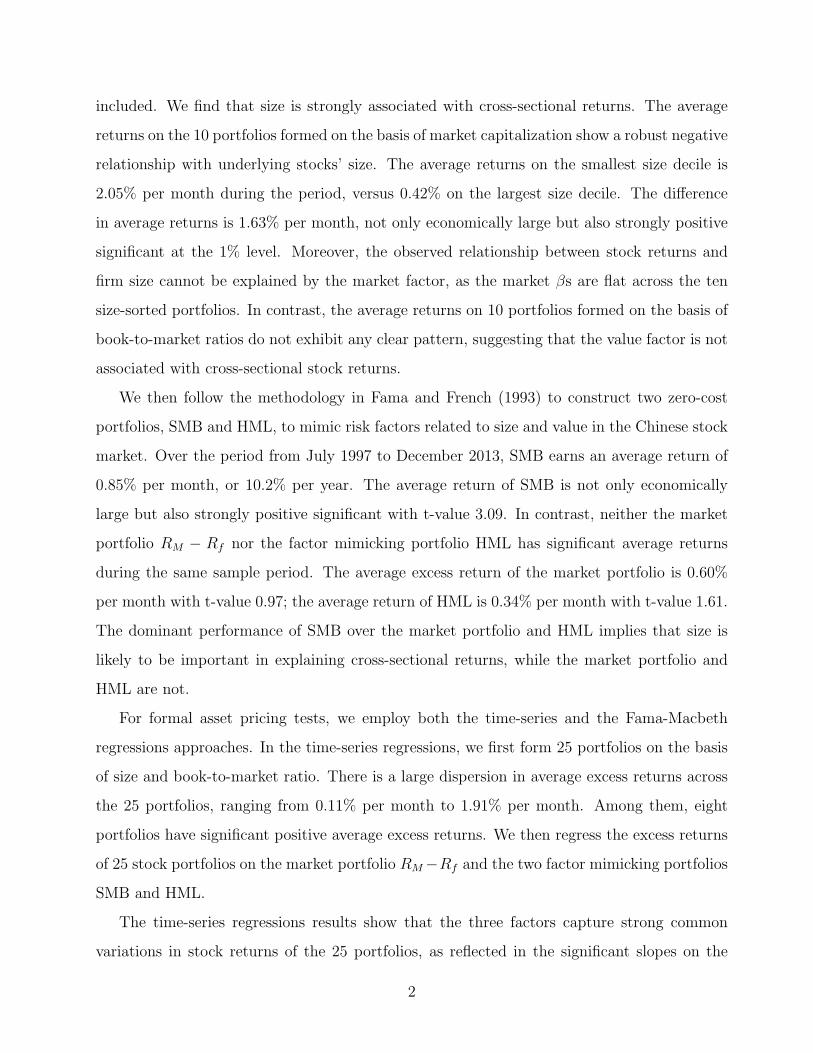
Figure 2 gives a graphic picture of the average returns across the 10 size and B/M ratio

sorted portfolios. In addition to average returns and their associated 95% confidence intervals,

we also plot a trend line through the average returns of the 10 ranked portfolios. The downward

sloping trend line in the top panel confirms the strong negative relation between returns and

size. By comparison, the upward sloping trend line in the bottom panel is much flatter.

4.2 Construction of the Size and Value Factor

To mimic underlying risk factors related to size and book-to-market ratios, we first construct

six portfolios by intersecting two size-sorted portfolios with three B/M-sorted portfolios. At

June of each year t, we form two size portfolios, Small and Big, by dividing all non-financial

stocks listed on the Shanghai and Shenzhen exchanges equally into two groups on the basis

of their floating A-share market capitalization. Similarly, three B/M portfolios are formed by

assigning all stocks into three groups by their book-to-market ratios: Low, Medium, and High.

The three subgroups represent the bottom 30%, middle 40%, and top 30%, respectively. The

two size-sorted portfolios and three B/M-sorted portfolios produce six portfolios: Small-Low,

Small-Medium, Small-High, Big-Low, Big-Medium and Big-High. For example, the Small-Low

portfolio contains the stocks in the Small size group that are also in the Low book-to-market

group. Monthly value-weighted returns on the six portfolios are calculated from July of year t

to June of t+ 1, where the weight for each stock is its floating A-share market capitalization.

12

-1.0

-0.5

0.0

0.5

1.0

1.5

2.0

2.5

3.0

3.5

4.0

4.5M

onth

ly E

xces

s R

etur

n

Small 2 3 4 5 6 7 8 9 Large

10 Size-sorted Groups

Trend LineAverage Excess Return (with 95% confidence level)

-1.0

-0.5

0.0

0.5

1.0

1.5

2.0

2.5

3.0

3.5

4.0

4.5

Mon

thly

Exc

ess

Ret

urn

Low 2 3 4 5 6 7 8 9 High

10 B/M-sorted Groups

Trend LineAverage Excess Return (with 95% confidence level)

Figure 2: Monthly excess returns of 10 size- and B/M-sorted portfolios.

The portfolios are reformed in June of t+ 1.4

We then construct two portfolios, SMB and HML, which mimic risk factors in returns

related to size and book-to-market ratios. SMB (small minus big) is the difference between the

4We follow the existing literature to sort firms into three groups on B/M ratios and only two on size. Themain consideration for the split is to be consistent with the classic Fama-French factors for the U.S. market.Given that the size effect is actually stronger in the Chinese market, we also consider two different splits inrobustness check section. The results remain similar.

13

simple average of the returns on the three small-stock portfolios (Small-Low, Small-Medium

and Small-High) and the three big-stock portfolios (Big-Low, Big-Medium and Big-High).

Since the two components of SMB are returns on small and big-stock portfolios with about the

same weighted-average book-to-market ratios, SMB captures the different returns behaviors

of small and big stocks and is largely free of the influence related to book-to-market ratios.

Similarly, we construct a HML (high minus low) portfolio which is the difference between the

simple average of the returns on the two high B/M portfolios (Small-High and Big-High) and

the two low B/M portfolios (Small-Low and Big-Low).

Table 2 summarizes the returns of the market factor, SMB and HML. In the A-share

Chinese market, the average value of market excess returns RM − Rf is 0.60% per month

from July 1997 to December 2013. The magnitude is large, equivalent to 7.2% annualized

returns, but with t-statistics at only 0.97 and not statistically significant. SMB, the size

factor mimicking portfolio, has average monthly returns of 0.85% which translates to 10.2%

annual returns. The magnitude is not only economically large but also strongly statistically

significant with t-value 3.09. By comparison, the mimicking portfolio for book-to-market

ratios, HML, produces an average returns of 0.34% per month, but with t-value of only 1.61.

Among the three factors for the Chinese market (RM − Rf , SMB and HML), SMB has the

largest average returns and is the only one that is statistically significant, highlighting the

strong size effect in Chinese stock returns.

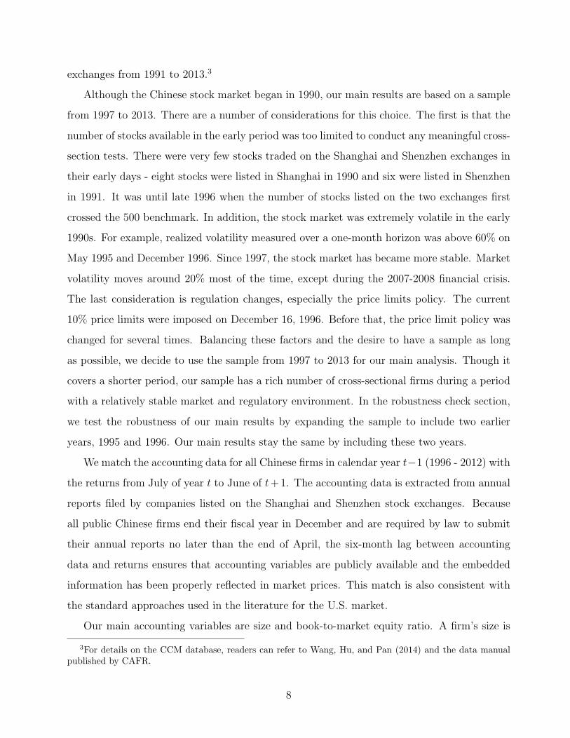
The dominant performance of SMB over another two factors is also clear in Figure 3, which

plots the accumulated value of investing 1 RMB at the end of June 1997 over the sample period

from July 1997 to December 2013.

To draw a parallel between the factors of the Chinese market and that of the U.S. market,

we put the summary statistics of the three factors we constructed for the Chinese market

along with those in the U.S. market. Since one concern of our study is that our sample period

covers only 198 months from July 1997 to December 2013 , we report summary statistics

for the three factors in the U.S. market separately for two sample periods: One is the same

sample period from July 1997 to December 2013 and another one is a much longer period

since 1962 (July 1962- December 2013). For the factors of the U.S. market, the average excess

returns from July 1962 to December 2013 is 0.53% per month for the market portfolio; 0.24%

14

Table 2: Summary Statistics of RM −Rf , SMB, HML and the Six Size-B/M Sorted Portfolios

RM −Rf SMB HML Small-Low Small-Medium Small-High Big-Low Big-Medium Big-High

Panel A: China’s A share market: July 1997 - December 2013

mean 0.60 0.85*** 0.34 1.18* 1.44** 1.47** 0.32 0.53 0.70T [0.97] [3.09] [1.61] [1.69] [2.07] [2.04] [0.52] [0.81] [1.07]std 8.63 3.86 2.95 9.79 9.77 10.20 8.66 9.17 9.21skewness 0.37 −0.28 0.28 0.33 0.27 0.35 0.55 0.26 0.56

Panel B: The U.S. market: July 1997 - December 2013

mean 0.49 0.32 0.26 0.59 0.95** 1.03** 0.49 0.53 0.58T [1.44] [1.25] [1.08] [1.12] [2.34] [2.41] [1.48] [1.57] [1.54]std 4.77 3.61 3.44 7.37 5.70 6.02 4.68 4.78 5.30skewness −0.68 0.87 0.01 −0.19 −0.50 −0.67 −0.58 −0.64 −0.79

Panel C: The U.S. market: July 1962 - December 2013

mean 0.53*** 0.24** 0.38*** 0.53* 0.91*** 1.08*** 0.51*** 0.55*** 0.73***T [2.93] [1.96] [3.33] [1.92] [4.15] [4.77] [2.69] [3.18] [3.85]std 4.49 3.09 2.86 6.88 5.45 5.61 4.67 4.34 4.69skewness −0.52 0.54 −0.01 −0.35 −0.49 −0.39 −0.34 −0.36 −0.39

The summary statistics of monthly excess returns on RM − Rf , SMB, HML and the six size-B/M sortedportfolios are reported, separately for the Chinese and the U.S. stock markets. RM −Rf is the excess returnon a value weighted market portfolio, in which the weights are stocks’ floating A-share market capital. AtJune of each year t, six size-B/M double sorted portfolios are formed by intersecting two size portfolios (Smalland Big) and three value portfolios (Low, Medium and High). The summary statistics are calculated basedon the excess returns on the six portfolios: Small-Low, Small-Medium, Small-High, Big-Low, Big-Mediumand Big-High. SMB (small minus big) is the difference between the simple averages of the returns on thethree small-stock portfolios (Small-Low, Small-Medium and Small-High) and the three big-stock portfolios(Big-Low, Big-Medium and Big-High). HML (high minus low) is the difference between the simple averagesof the returns on the two high-B/M portfolios (Small-High and Big-High) and the two low-B/M portfolios(Small-Low and Big-Low). Mean is the time-series mean of a monthly returns, std is its time-series standarddeviation, T is mean divided by its time-series standard error, and skewness is the time-series skewness ofmonthly returns.

per month for SMB; 0.38% per month for HML. Except SMB which has a marginal t-value

of 1.96, both the market and HML factor of the U.S. market have significant positive average

returns. In contrast, for the shorter period from July 1997 to December 2013, none of the

three U.S. factors is significant. The lack of statistical significance of the three U.S. factors

during the shorter period underscores biases of cross-sectional pricing tests on small samples.

To mitigate the potential small sample effect for our tests on the Chinese market, we perform

a robustness check by including two more years 1995 and 1996 in our sample. However, given

the short history of the Chinese stock market, we admit that our results are unavoidably

limited by the small sample.

The correlation structure of the three Chinese returns factors is very different from those

in the U.S. market. As seen in Table 3, among the three Chinese factors, only the market

15

0.0

0.5

1.0

1.5

2.0

2.5

3.0

3.5

4.0

4.5

5.0

5.5

Accu

mu

lati

ve

Re

turn

Jul1997 Jul1999 Jul2001 Jul2003 Jul2005 Jul2007 Jul2009 Jul2011 Jul2013

Market Excess Return

HML

SMB

Figure 3: Accumulative returns of RM −Rf , SMB and HML (July 1997 - December 2013)

and HML have significant correlation, 0.19 and statistically significant at the 1% level. On

the contrary, the three factors in the U.S. market are all strongly correlated with one another.

For the same time period from 1997 to 2013, the correlation is 0.27 for the market factor and

SMB; -0.21 for the market factor and HML; -0.35 for SMB and HML. The correlations are

all statistically significant at the 1% level. The three U.S. factors exhibit similar correlations

over the longer period from 1962 to 2013. There is no strong cross-correlation between the

Chinese and U.S. market factors, with the exception that the Chinese market index tends to

move in the same direction with the U.S. market index.

4.3 Seasonality

The returns on the three factors, RM −Rf , SMB and HML exhibit strong seasonality. Table 4

summarizes the empirical pattern. For each month, we report the average excess returns as

well as the average number of trading days for the three factors and the six size- and B/M-

16

Tab

le3:

Correlation

sof

RM

−R

f,SMB

andHMLFactors

Pan

elA:pairw

isecorrelations

China’sstock

market:

1997-2013

U.S.stock

market:

1997-2013

U.S.stock

market:

1962-2013

RM

−R

fSMB

HML

RM

−R

fSMB

HML

RM

−R

fSMB

HML

RM

−R

f0.09

0.19***

0.27***

−0.21***

0.31***

−0.30***

SMB

0.05

−0.35***

−0.23***

Pan

elB:cross-correlationsbetweenthefactorsin

theChinesestock

marketan

dtheU.S.stock

market,1997-2013

RM

−R

US

fSM

BUS

HM

LUS

RM

−R

CH

f0.19***

0.09

-0.05

SM

BCH

-0.02

-0.12*

0.03

HM

LCH

-0.00

-0.02

0.07

Pan

elA

reportsthepairw

isecorrelationsofmon

thly

returnson

RM

−R

f,SMB

andHMLfactors

forthreesamples:

China’sstock

market

from

July

1997to

Decem

ber

2013,

U.S.stock

market

from

July

1997

toDecem

ber

2013andU.S.stock

market

from

July

1962to

Decem

ber

2013.Panel

Breports

thecross

correlationsof

RM

−R

f,SMB

andHMLin

China’sstock

market

andR

M−

Rf,SMB

andHMLin

theU.S.stock

market.*,

**an

d***

correspondto

statisticalsign

ificance

at10%,5%

and1%

,respectively.

17

sorted portfolios. The average number of days range from 14 to 22. The month with the

lowest number of trading days is February, due to the fact that long holidays for the Chinese

Lunar New Year often fall in this month. February is also the month when the market index

has the highest returns 3.45% and the only month when the market excess returns is positively

significant. Taking out February, the average market excess returns is 0.35% and only 0.53

standard errors from zero. Similar to the market factor, the six size- and B/M-sorted portfolios

also have the highest returns in February.

In February, March, May and August, small stocks out-perform large stocks and SMB

fetches significant positive excess returns. There is only one month, June, when small stocks

under-perform large stocks by a marginal negative significant -1.71% (with t-value -1.87).

SMB has a robust 2.77% returns in February, but its best performance of 3.07% occurs in

March. Taking out February, SMB has an average returns of 0.68% and is still significant at

the 5% level. HML doesn’t show strong seasonality. HML doesn’t have statistically significant

returns, positive or negative, in any of the calendar months.

5 Asset-Pricing Tests

5.1 Time-Series Regressions

For a formal asset-pricing test, we first employ the time-series regression approach of Jensen,

Black, and Scholes (1972) and Fama and French (1993). Monthly excess returns of stocks

are regressed on the excess returns to a market portfolio of stocks (RM −Rf ) and mimicking

portfolios for size (SMB) and book-to-market ratio (HML). If assets are priced rationally, the

slopes and R2 in the time-series regressions should reflect whether mimicking portfolios for the

risk factors related to size and B/M captures common variations in stock returns not explained

by the market factor. Moreover, the estimated intercepts in such regressions provide direct

evidence on how well the combined factors explain the cross-section of average returns.

We follow the literature to form 25 double-sorted portfolios. In June of each year t, we sort,

independently, all non-financial stocks listed on the Shanghai and Shenzhen exchanges to five

size and book-to-market quintiles. We then form the 25 portfolios from the intersections of the

size and B/M quintiles. The portfolios are kept unchanged for the next 12 months, from July

18

Tab

le4:

Seasonality

Portfolios

Jan

Feb

Mar

Apr

May

Jun

Jul

Aug

Sept

Oct

Nov

Dec

NoFeb

All

Pan

elA:returnsonR

M−

Rf,SMB

andHML

RM-R

f2.61

3.45***

1.25

2.16

1.74

−0.87

0.50

−2.16

−1.02

−1.24

0.35

0.81

0.35

0.60

[1.12]

[2.67]

[0.55]

[0.95]

[0.85]

[−0.26]

[0.23]

[−0.99]

[−0.74]

[−0.57]

[0.20]

[0.43]

[0.53]

[0.97]

SMB

0.78

2.77***

3.07***

−0.06

2.17***

−1.71*

0.83

2.55***

−0.13

−0.42

1.49

−1.06

0.68**

0.85***

[0.93]

[4.65]

[3.47]

[−0.07]

[2.63]

[−1.87]

[0.76]

[3.12]

[−0.16]

[−0.52]

[1.32]

[−1.12]

[2.33]

[3.09]

HML

0.73

1.18

1.00*

1.16*

−0.10

−0.82

1.20

−0.00

−0.34

0.40

−0.03

−0.26

0.26

0.34

[1.00]

[1.47]

[1.91]

[1.65]

[−0.12]

[−1.02]

[1.59]

[−0.00]

[−0.60]

[0.57]

[−0.06]

[−0.37]

[1.22]

[1.61]

Tradingday

s18

1422

21

1921

22

22

2118

2122

2120

Pan

elB:excess

returnsonthesixsize-B

/Msorted

portfolios

Small-Low

3.58

5.77***

2.78

1.37

3.69

−2.54

1.19

−0.05

−0.68

−2.31

2.05

−0.28

0.77

1.18*

[1.32]

[3.49]

[1.05]

[0.51]

[1.64]

[−0.80]

[0.49]

[−0.02]

[−0.38]

[−1.04]

[1.01]

[−0.12]

[1.05]

[1.69]

Small-Medium

3.43

6.66***

3.34

2.06

4.21*

−3.13

1.67

0.06

−0.91

−2.21

2.37

0.16

0.98

1.44**

[1.37]

[3.84]

[1.25]

[0.78]

[1.77]

[−1.00]

[0.64]

[0.03]

[−0.55]

[−1.01]

[1.16]

[0.07]

[1.34]

[2.07]

Small-High

3.87

7.19***

3.96

2.30

4.01

−3.34

2.18

0.33

−1.02

−2.21

1.57

−0.61

0.97

1.47**

[1.58]

[3.94]

[1.40]

[0.78]

[1.64]

[−0.92]

[0.81]

[0.13]

[−0.60]

[−1.02]

[0.79]

[−0.28]

[1.28]

[2.04]

Big-Low

2.14

3.18**

−0.28

1.12

2.12

−0.36

−0.17

−2.33

−0.70

−2.07

0.53

1.01

0.07

0.32

[0.87]

[2.30]

[−0.13]

[0.52]

[1.07]

[−0.10]

[−0.09]

[−1.12]

[−0.47]

[−0.89]

[0.26]

[0.48]

[0.11]

[0.52]

Big-M

edium

3.09

4.01***

0.59

2.30

1.67

−2.33

1.47

−2.27

−0.47

−2.02

0.07

0.63

0.22

0.53

[1.29]

[2.76]

[0.25]

[0.92]

[0.84]

[−0.69]

[0.62]

[−0.99]

[−0.29]

[−0.91]

[0.03]

[0.30]

[0.32]

[0.81]

Big-H

igh

3.31

4.11***

0.56

2.51

1.61

−1.19

1.26

−2.71

−1.04

−1.39

0.94

0.82

0.40

0.70

[1.48]

[3.04]

[0.25]

[1.01]

[0.70]

[−0.31]

[0.52]

[−1.14]

[−0.73]

[−0.66]

[0.51]

[0.42]

[0.57]

[1.07]

Panel

Areportsthetime-series

averages

andtheassociated

t-values

ofreturnsonR

M−R

f,SMB

andHML,separatelyforeach

calendar

mon

thfrom

July

1997to

Decem

ber

2013.Theaveragenumber

oftradingday

sin

each

calendar

mon

this

alsoreported.Pan

elB

reports

thetime-series

averages

andthet-values

forexcess

returnson

thesixsize-B

/M

sorted

portfoliosfrom

July

1997to

Decem

ber

2013.*,

**an

d***

correspon

dto

statistical

sign

ificance

at10%

,5%

and1%,respectively.

19

of year t to June of year t+ 1. We calculate monthly portfolio returns as the value-weighted

average of individual stocks in each portfolio, in which the weights are the floating A-share

market capitalization.

Table 5 summarizes characteristics of companies in the 25 double-sorted portfolios. The

double sorting produces a wide spread in size and B/M ratios. Across the 25 portfolios,

average size ranges from 591 million RMB to 11.9 billion RMB and average B/M ratio range

from 0.15 to 0.70. The average number of firms in each portfolio varies from 19.4 for the

smallest-size and highest-B/M ratio portfolio to 55.1 for the largest-size and highest-B/M

ratio portfolio. Controlling for size, high B/M portfolios tend to have high market leverage

(A/ME) and low book leverage (A/BE). They also have high dividend yields and E/P ratios.

These are generally in line with patterns in the U.S. market. In addition, average floating

ratios increase from the small- to large-size portfolios in each of the B/M quintiles, with

differences range from 0.14 to 0.18. Average floating ratios also rise as B/M ratio increases,

though the magnitudes are smaller. In other words, large and value firms also tend to be

those with higher percentage of floating share in the Chinese market.

For each of the 25 size-B/M sorted portfolios, we run the following regressions:

Rpt −Rf,t = αp + βM

p (RM,t −Rf,t) + βSMBp SMBt + βHML

p HMLt + ϵpt , (1)

where Rpt −Rf,t is the excess returns on the portfolio at month t, RM,t−Rf,t is excess returns

of the value-weighted Chinese market index, SMBt and HMLt are returns on two zero-cost

factor-mimicking portfolios for size and book-to-market, respectively. Table 6 summarizes the

excess returns and time-series regression results. There is a large dispersion in average excess

returns across the 25 portfolios, from 0.11% to 1.91%. Consistent with the patterns for the

univariate sorted portfolios, average returns and size show a clear negative relation. In each of

the B/M quintiles, excess returns monotonically decrease from the smaller- to the larger-size

portfolios. By comparison, the relation between average returns and book-to-market equity

is much weaker. Though average returns show a tendency to rise as B/M ratios increase,

the pattern is not monotonic and often very flat. It’s worth emphasizing that only small-size

stocks have significant positive excess returns in the Chinese market in our sample of July 1997

to December 2013. None of the portfolios in the top three size quintiles has excess returns

20

Table 5: Summary Statistics For 25 Portfolios Formed on Size and Book-to-Market Ratios(July 1997 - December 2013)

B/M Quitile

Size Quintile Low 2 3 4 High High-Low Low 2 3 4 High High-Low

ME(in million) B/M ratio

Small 591 596 618 620 643 52*** 0.15 0.27 0.35 0.45 0.60 0.45***2 991 973 1,022 1,012 1,019 28*** 0.16 0.27 0.35 0.45 0.63 0.46***3 1,454 1,488 1,467 1,472 1,476 22** 0.17 0.27 0.35 0.45 0.65 0.48***4 2,388 2,335 2,319 2,399 2,298 −90*** 0.17 0.27 0.35 0.45 0.66 0.49***Big 9,072 7,433 7,709 11,920 10,888 1,816*** 0.16 0.27 0.35 0.45 0.70 0.54***Big−Small 8,480*** 6,838*** 7,090*** 11,301*** 10,245*** 0.01 −0.00 0.00 0.00 0.10

% of market value in portfolio N

Small 1.36 1.30 1.29 0.90 0.51 −0.85*** 53.4 53.3 52.1 42.8 19.4 −33.9***2 1.48 1.71 1.99 1.91 1.51 0.04 41.2 45.0 48.6 47.5 39.5 −1.83 1.88 2.29 2.44 2.69 2.82 0.94*** 36.0 41.8 44.4 47.2 52.7 16.8***4 3.12 3.41 3.21 3.95 4.50 1.38*** 41.0 40.9 40.1 45.2 54.8 13.8***Big 12.83 9.09 8.68 10.60 14.53 1.70** 49.5 41.0 36.8 39.3 55.1 5.5***Big−Small 11.48*** 7.78*** 7.39*** 9.69*** 14.02*** −3.8 −12.3*** −15.4*** −3.5* 35.7***

βM Floating ratio

Small 1.03*** 1.04*** 1.04*** 1.05*** 1.10*** 0.06** 0.39 0.37 0.39 0.40 0.43 0.04***2 1.03*** 1.01*** 1.04*** 1.11*** 1.07*** 0.04 0.46 0.46 0.48 0.51 0.52 0.06***3 0.99*** 1.05*** 1.06*** 1.06*** 1.10*** 0.11*** 0.49 0.51 0.52 0.54 0.56 0.07***4 0.96*** 1.03*** 1.07*** 1.07*** 1.09*** 0.12*** 0.50 0.53 0.55 0.56 0.57 0.07***Big 0.99*** 1.04*** 1.09*** 1.06*** 1.08*** 0.09** 0.55 0.55 0.55 0.57 0.57 0.02***Big−Small −0.04 −0.01 0.05 0.01 −0.02 0.16*** 0.18*** 0.16*** 0.17*** 0.14***

A/BE A/ME

Small 5.66 1.98 1.89 1.88 1.88 −3.77*** 0.46 0.54 0.68 0.86 1.15 0.69***2 3.30 2.00 1.93 2.00 2.06 −1.24*** 0.42 0.55 0.70 0.92 1.32 0.90***3 3.53 2.08 2.05 2.02 2.11 −1.42*** 0.37 0.57 0.74 0.94 1.42 1.05***4 2.61 2.01 2.07 2.03 2.04 −0.57*** 0.39 0.57 0.75 0.95 1.39 1.00***Big 2.22 2.01 2.07 2.11 2.16 −0.06*** 0.36 0.54 0.75 0.98 1.55 1.20***Big−Small −3.44 0.03 0.18 0.23 0.27 −0.10 0.00 0.07 0.12 0.40

E/P ratio D/P ratio

Small 1.58 1.87 2.07 2.12 2.12 0.54*** 0.11 0.33 0.50 0.54 0.45 0.34***2 1.94 2.01 2.32 2.52 2.48 0.54*** 0.21 0.37 0.47 0.52 0.57 0.36***3 1.89 2.46 2.80 2.98 2.96 1.06*** 0.24 0.47 0.65 0.70 0.80 0.56***4 2.31 2.63 3.11 3.32 3.61 1.30*** 0.38 0.58 0.66 0.79 0.82 0.44***Big 2.67 3.50 4.04 4.59 4.92 2.25*** 0.42 0.71 0.96 1.04 1.17 0.75***Big−Small 1.09 1.64 1.97 2.48 2.80 0.31 0.38 0.46 0.50 0.72

Average characteristics of 25 size-B/M portfolios are reported. Variable are defined in Table 1. The 25portfolios are formed at the end of each June from 1997 to 2012, by intersecting five size-sorted portfoliosand five B/M sorted portfolios. *, ** and *** correspond to statistical significance at 10%, 5% and 1%,respectively.

significant at the 5% level. For the remaining 10 portfolios in the bottom two size quintiles,

eight portfolios have excess returns significant at the 5% level, with t-values from 2.04 to 2.57.

Slopes on the market excess returns, βMs, are all strongly statistically significant with

t-values close or above 40.0. Unlike the U.S. market, βMs across the 25 portfolios are much

flatter, with variation less than 0.1. More importantly, βMs show no relation with size and

B/M ratios. Thus, the market factor can help explain the overall magnitude of average excess

21

Table 6: Time-Series Regressions of Excess returns of 25 Size-B/M Sorted Portfolios on RM −Rf , SMB and HML (July 1997 - December 2013)

B/M Quitile

Size Quintile Low 2 3 4 High Low 2 3 4 High

Portfolio excess return Abnormal return: αp

Small 1.66** 1.61** 1.75** 1.91** 1.74** 0.08 0.04 0.20 0.26 0.03[2.25] [2.19] [2.39] [2.57] [2.26] [0.45] [0.26] [1.28] [1.43] [0.17]

2 0.90 1.31* 1.43** 1.70** 1.47** −0.28 0.11 0.05 0.19 −0.03[1.30] [1.94] [2.05] [2.27] [2.04] [−1.56] [0.71] [0.26] [1.07] [−0.18]

3 0.79 1.14* 1.07 1.01 1.26* −0.20 0.01 −0.09 −0.23 −0.15[1.22] [1.65] [1.55] [1.45] [1.72] [−1.08] [0.06] [−0.51] [−1.36] [−0.85]

4 0.48 0.72 0.76 0.91 0.88 −0.26 −0.11 −0.26 −0.15 −0.21[0.75] [1.08] [1.10] [1.30] [1.25] [−1.19] [−0.53] [−1.37] [−0.74] [−1.19]

Big 0.19 0.11 0.44 0.66 0.49 0.14 −0.23 −0.08 0.12 −0.03[0.29] [0.17] [0.65] [1.00] [0.76] [0.86] [−1.27] [−0.44] [0.71] [−0.17]

Coefficients of RM,t −Rf,t: βMp Coefficients of SMB: βSMB

p

Small 0.99*** 1.01*** 1.01*** 0.99*** 1.03*** 1.29*** 1.23*** 1.20*** 1.18*** 1.14***[48.85] [57.15] [55.58] [48.14] [44.28] [29.10] [31.90] [30.08] [26.06] [22.34]

2 1.02*** 0.99*** 0.98*** 1.06*** 1.00*** 0.87*** 0.87*** 0.96*** 0.95*** 0.94***[48.25] [52.71] [46.98] [50.53] [50.57] [18.68] [21.09] [20.76] [20.72] [21.73]

3 0.96*** 1.02*** 1.02*** 1.03*** 1.03*** 0.70*** 0.71*** 0.68*** 0.72*** 0.73***[44.21] [44.49] [49.30] [51.95] [50.20] [14.61] [14.06] [14.99] [16.63] [16.24]

4 0.98*** 1.01*** 1.05*** 1.04*** 1.05*** 0.42*** 0.42*** 0.50*** 0.45*** 0.40***[38.99] [41.23] [48.50] [44.78] [51.87] [7.52] [7.81] [10.52] [8.75] [9.03]

Big 1.02*** 1.02*** 1.07*** 1.01*** 0.97*** −0.30*** −0.21*** −0.12** −0.24*** −0.33***[52.58] [49.51] [49.45] [54.41] [52.44] [−7.09] [−4.61] [−2.53] [−5.75] [−8.23]

Coefficients of HML: βHMLp R2

Small −0.30*** −0.23*** −0.19*** 0.19*** 0.38*** 0.95 0.96 0.96 0.95 0.94[−5.06] [−4.40] [−3.67] [3.09] [5.67]

2 −0.45*** −0.37*** −0.03 0.20*** 0.32*** 0.94 0.95 0.94 0.95 0.95[−7.29] [−6.75] [−0.50] [3.22] [5.56]

3 −0.50*** −0.24*** −0.09 0.06 0.50*** 0.92 0.92 0.94 0.94 0.94[−7.82] [−3.54] [−1.54] [0.99] [8.32]

4 −0.58*** −0.39*** −0.10 0.16** 0.34*** 0.89 0.9 0.93 0.92 0.94[−7.92] [−5.50] [−1.53] [2.32] [5.82]

Big −0.93*** −0.29*** −0.04 0.41*** 0.67*** 0.94 0.93 0.93 0.94 0.94[−16.27] [−4.82] [−0.65] [7.54] [12.38]

For each of the 25 size-B/M sorted portfolios, we run the regression: Rpt − Rf,t = αp + βM

p (RM,t − Rf,t) +

βSMBp SMBt+βHML

p HMLt+ϵpt , whereRpt−Rf,t is the excess return on the portfolio at month t, RM,t−Rf,t is

excess return on the market index RM−Rf , SMBt and HMLt are returns on two zero-cost factor-mimickingportfolios for size and book-to-market ratio, respectively. *, ** and *** correspond to statistical significanceat 10%, 5% and 1%, respectively.

returns of each portfolio, but it cannot explain the wide variations related to size and B/M

ratios. By contrast, slopes on SMB and HML are not only statically significant but also keep

the orderings of the corresponding size and book-to-market ratios. Slopes on SMB, with a large

spread of 1.62, decreases as portfolio sizes move from the smallest quintile to the largest. The

t-values for small-size stocks are also generally larger in magnitudes than large-size stocks. All

slopes on SMB are strongly significant, even the least significant one is -2.53 standard errors

from zero. Similar to the slopes on SMB, slopes on HML are also monotonically related to

22

B/M ratios within each of the size quintiles. The significance of the slopes on HML, however,

is much weaker than both the market βMs and the slopes on SMB. For example, four out of

five portfolios in the middle B/M quintile don’t have significant exposure to the HML factor.

R-squared across the 25 portfolios are quite high, from 89% to 96%.

We then turn to the most important metrics, αs, which are intercepts of the time-series

regressions on the excessive returns of the 25 size and B/M sorted portfolios. The results

are encouraging - all of the αs are small in magnitudes and non-significant from zeros. In

addition, the remaining αs show no relation with neither size nor B/M ratios. Judging on the

basis of the intercepts, the three factors, Market, SMB and HML, successfully capture the

cross-section of average returns. Moreover, given the flat structure of market βMs, the returns

variations related to size and book-to-market ratios are more likely to be driven by exposures

to the two factor mimicking portfolios, SMB and HML.

To separate roles played by each of the three factors, we report intercepts for different

model setups in Table 7. When the market excess returns is used alone to explain portfolio

excess returns in the time-series regressions, the intercepts αs are smaller than the average

excess returns, but remain strongly significant. In fact, Ten out of the 25 portfolios still have

positive significant αs and one portfolio has negative significant α. In addition, the remaining

αs still maintain the cross-section pattern with size and B/M ratios. In contrast, using SMB

as the sole factor makes all intercepts in the time-series regressions non-significant from zeros.

More important, after taking out the exposures to the SMB factor, the remaining intercepts

no longer monotonically decreases with respect to size. However, that even though no α is

statistically significant, 24 out of the 25 αs remain positive, and the highest α is at 0.74% per

month. Next, we combine SMB with the market factor. The intercepts are further reduced

in magnitude and remain non-significant for the majority of the portfolios. Out of the total

25 portfolios, only one portfolio has intercept, -0.41%, significant at the 5% level. HML, on

the other hand, is not very successful in explaining cross-section returns. Whether used alone

or in combination with the market factor, the intercepts for portfolios in the bottom two size

quintiles remain large and statistically significant. Putting all evidence together, it is clear

that SMB is the most important factor in terms of explaining cross-section returns in China’s

stock market.

23

Table 7: Intercepts From Excess Stock returns Regressions for 25 Stock Portfolios Formed onSize and Book-to-Market Ratios (July 1997 - December 2013)

B/M Quitile

Size Quintile Low 2 3 4 High Low 2 3 4 High

Rpt = αp + βM

p (RM,t −Rf,t) + ϵpt Rpt = αp + βSMB

p SMBt + βHMLp HMLt + ϵpt

Small 1.05*** 0.99*** 1.13*** 1.28*** 1.08*** 0.34 0.30 0.47 0.52 0.30[2.66] [2.67] [3.11] [3.46] [2.86] [0.53] [0.47] [0.72] [0.80] [0.45]

2 0.29 0.72** 0.82*** 1.04*** 0.84*** −0.02 0.37 0.31 0.47 0.23[0.95] [2.46] [2.61] [3.25] [2.66] [−0.03] [0.59] [0.48] [0.69] [0.36]

3 0.22 0.52* 0.44* 0.38 0.60** 0.05 0.28 0.18 0.04 0.12[0.79] [1.89] [1.73] [1.46] [2.10] [0.08] [0.42] [0.27] [0.06] [0.18]

4 −0.09 0.12 0.13 0.27 0.22 −0.00 0.15 0.02 0.13 0.07[−0.34] [0.47] [0.55] [1.14] [1.04] [−0.00] [0.23] [0.03] [0.18] [0.10]

Big −0.38 −0.49** −0.19 0.04 −0.10 0.41 0.04 0.20 0.38 0.23[−1.43] [−2.52] [−1.04] [0.23] [−0.46] [0.63] [0.06] [0.29] [0.59] [0.37]

Rpt = αp + βSMB

p SMBt + ϵpt Rpt = αp + βHML

p HMLt + ϵpt

Small 0.41 0.41 0.58 0.74 0.59 1.54** 1.46** 1.60** 1.63** 1.38*[0.65] [0.63] [0.89] [1.13] [0.85] [2.08] [1.98] [2.17] [2.24] [1.86]

2 0.02 0.43 0.46 0.71 0.50 0.84 1.23* 1.23* 1.40* 1.15[0.03] [0.68] [0.72] [1.02] [0.75] [1.19] [1.80] [1.77] [1.92] [1.65]

3 0.06 0.38 0.32 0.23 0.45 0.76 1.00 0.88 0.78 0.87[0.10] [0.57] [0.48] [0.34] [0.64] [1.16] [1.46] [1.29] [1.13] [1.25]

4 −0.01 0.20 0.17 0.35 0.35 0.48 0.64 0.58 0.64 0.55[−0.02] [0.31] [0.24] [0.50] [0.50] [0.74] [0.97] [0.84] [0.94] [0.81]

Big 0.31 0.12 0.37 0.67 0.59 0.31 0.01 0.25 0.33 0.09[0.47] [0.19] [0.53] [1.00] [0.89] [0.48] [0.02] [0.38] [0.52] [0.15]

Rpt = αp + βM

p (RM,t −Rf,t) + βSMBp SMBt + ϵpt Rp

t = αp + βMp (RM,t −Rf,t) + βHML

p HMLt + ϵpt

Small −0.00 −0.02 0.15 0.31* 0.14 1.12*** 1.04*** 1.17*** 1.21*** 0.95**[−0.02] [−0.14] [0.91] [1.68] [0.65] [2.84] [2.79] [3.20] [3.27] [2.57]

2 −0.41** 0.01 0.04 0.25 0.06 0.41 0.82*** 0.82** 0.96*** 0.73**[−1.99] [0.08] [0.21] [1.34] [0.31] [1.39] [2.84] [2.58] [3.04] [2.36]

3 −0.34 −0.05 −0.12 −0.22 −0.01 0.36 0.58** 0.46* 0.35 0.44*[−1.58] [−0.26] [−0.65] [−1.28] [−0.07] [1.35] [2.12] [1.79] [1.35] [1.66]

4 −0.42* −0.22 −0.28 −0.11 −0.11 0.08 0.23 0.15 0.21 0.12[−1.68] [−0.97] [−1.51] [−0.52] [−0.61] [0.32] [0.96] [0.64] [0.92] [0.57]

Big −0.11 −0.31 −0.09 0.23 0.16 −0.10 −0.40** −0.18 −0.07 −0.30[−0.42] [−1.64] [−0.50] [1.25] [0.73] [−0.54] [−2.16] [−0.96] [−0.44] [−1.64]

The excess returns on 25 stock portfolios formed on size and book-to-market ratios are regressed in sixdifferent models. The estimated intercepts αp and the associated t-values for each portfolio are reported. *,** and *** correspond to statistical significance at 10%, 5% and 1%, respectively.

We also perform the Gibbons, Ross and Shanken F-tests to formally test whether the

intercepts for the 25 stock portfolios are jointly zero in different models. Table 8 reports the

F-statistics and the associated probability levels. The three stock-market factors, RM − Rf ,

SMB, and HML, produce the smallest F-statistic 0.93 with a bootstrap probability of 0.40.

Thus, we can not reject the hypothesis that the intercepts for the 25 portfolios are all zero

in a three-factor model. However, it is worth noting that F-tests can not reject the joint-

zero intercepts hypothesis for any of the models. The F-statistic for the CAPM model is the

largest, 1.33 with a bootstrap probability of 0.85. Thus, even though 11 out of 25 portfolios

24

have significant intercepts under the CAPM model, the F-test couldn’t reject the hypothesis

that the intercepts are jointly zero. This is largely due to the fact that large Chinese stocks

don’t earn significant excess returns in general. In fact, only eight portfolios in the bottom

two size quintiles can produce significant excess returns. Given the lack of statistical power

of F-tests in the Chinese stock market, we rely more on the magnitude of the F-statistics to

judge the performance of different factors models. Within the three one-factor models, SMB

generates the lowest F-test statistic 1.01. Within the three two-factor models, the combination

of SMB and HML generates the lowest F-test statistic of 0.93. Thus, by all metrics, SMB is

the most important factor in explaining cross-sectional returns in China’s stock market.

Table 8: F-statistics and Matching Probability Levels of Bootstrap and F-distributions

Panel A: China’s stock market, July 1997 to December 2013(1) (2) (3) (4) (5) (6) (7)

F−statistics 0.93 1.00 1.23 0.93 1.33 1.01 1.25Probability level

Bootstrap 0.403 0.501 0.751 0.382 0.823 0.475 0.750F−distribution 0.435 0.532 0.783 0.434 0.850 0.547 0.800

Panel B: U.S. stock market, July 1997 to December 2013(1) (2) (3) (4) (5) (6) (7)

F−statistics 2.44 2.59 2.52 2.09 2.63 2.22 2.23Probability level

Bootstrap 0.996 0.998 0.995 0.986 0.998 0.992 0.989F−distribution 1.000 1.000 1.000 0.997 1.000 0.998 0.999

Seven different factor models are tested: (1) Rpt = αp + βM

p RMt + βSMB

p SMBt + βHMLp HMLt + ϵpt ; (2)

Rpt = αp + βM

p RMt + βSMB

p SMBt + ϵpt ; (3) Rpt = αp + βM

p RMt + βHML

p HMLt + ϵpt ; (4) Rpt = αp +

βSMBp SMBt + βHML

p HMLt + ϵpt ; (5) Rpt = αp + βM

p RMt + ϵpt ; (6) Rp

t = αp + βSMBp SMBt + ϵpt and (7)

Rpt = αp + βHML

p HMLt + ϵpt . Panel A reports the F-test results on the hypothesis that the intercepts, αs,are jointly zero across the 25 size-B/M sorted portfolios in the Chinese stock market, from July 1997 toDecember 2013. Panel B reports the F-test results for the U.S. market, from July 1997 to December 2013.

5.2 Fama-Macbeth Regressions

For asset pricing tests in this section, we follow the standard cross-sectional regression ap-

proach of Fama and MacBeth (1973). In the first-stage of the Fama-Macbeth regressions,

we estimate individual stocks’ exposures to the market, SMB and HML factors. To reduce

noises in the estimation, we follow the literature and use a portfolio-based approach. At the

25

end of June each year, we divided all non-financial stocks into three equal-sized portfolios by

individual stocks’ sizes and three equal-sized portfolios by their book-to-market ratios. We

then form nine double-sorted portfolios by intersecting the three size-sorted portfolios with the

three B/M-sorted portfolios. For each of the nine portfolios, we further divide each portfolio

into three portfolios using the pre-ranking CAPM βs of individual stocks, estimated with the

previous five years (with at least two years) of monthly returns. For each of the 27 portfolios,

the post-ranking betas are estimated by:

Rpt −Rf,t = αp+βM

p (RM,t−Rf,t)+βSMBp SMBt+βHML

p HMLt+ ϵpt , p = 1, 2, . . . , 27. (2)

where Rpi is the equal-weighted return for portfolio p in month t and this regression is run

over the entire sample period from July 1997 to December 2013. We then use each portfolio’s

full-sample post-ranking betas as the estimates for the individual stocks’ betas on market,

SMB and HML.

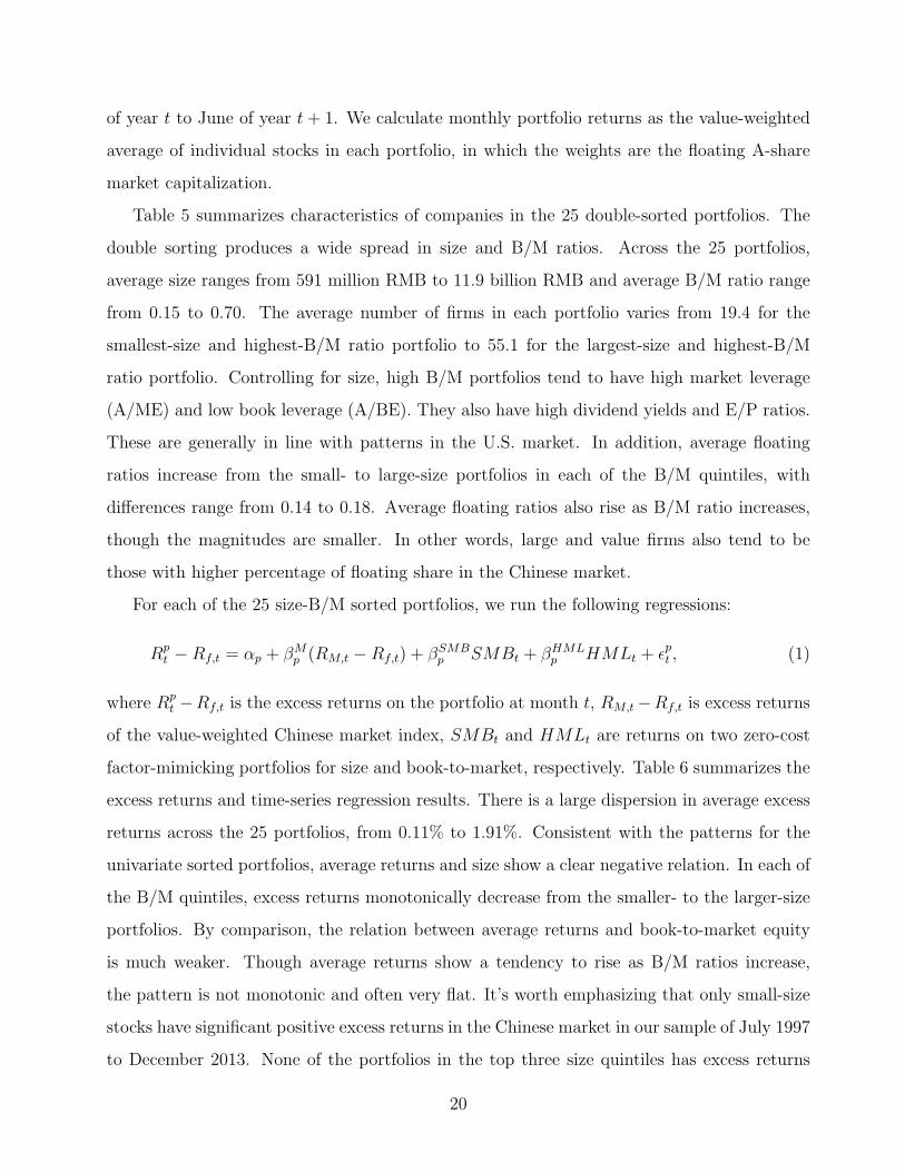
In the second stage of the Fama-Macbeth regressions, we run a cross-sectional regression

at each month t:

Rit −Rf,t = γ0,t + γM

t βMi + γSMB

t βSMBi + γHML

t βHMLi + ϵit, (3)

where Rit − Rf,t is the excess returns of stock i at month t, βM

i , βSMBi and βHML

i are our

estimates of stock i’s betas on market, SMB and HML, respectively. Figure 4 plots the

estimated factor premiums, γMt , γSMB

t and γHMLt , and the associated 95% confidence interval

of each month.

In a standard Fama-Macbeth regression, the factor premiums are estimated as the time-

series average of γMt , γSMB

t and γHMLt . That is:

γM,EW =N∑t=1

1

NγMt ,

γSMB,EW =N∑t=1

1

NγSMBt ,

γHML,EW =N∑t=1

1

NγHMLt ,

(4)

where N is the total number of months for the full sample period. In other words, the factor

26

-70

-60

-50

-40

-30

-20

-10

0

10

20

30

40

50

60

70

80

90

100

Slop

es o

n Rm

-Rf

1995 1997 1999 2001 2003 2005 2007 2009 2011 2013

July, 1997

Slopes on Rm-Rf (in percent, with 95% confidence level)

-25

-20

-15

-10

-5

0

5

10

15

20

25

30

35

40

45

50

55

60

Slop

es o

n SM

B

1995 1997 1999 2001 2003 2005 2007 2009 2011 2013

July, 1997

Slopes on SMB (in percent, with 95% confidence level)

-25

-20

-15

-10

-5

0

5

10

15

20

25

30

35

40

45

50

55

60

Slop

es o

n HM

L

1995 1997 1999 2001 2003 2005 2007 2009 2011 2013

July, 1997

Slopes on HML (in percent, with 95% confidence level)

Figure 4: Month-by-Month slopes on RM − Rf , SMB and HML in cross-sectional Fama-Macbeth regressions: July 1995 - December 2013

27

premiums are calculated as the equal-weighted averages of the estimated premiums of each

month.

In our sample of Chinese stocks, the earlier period contains much fewer number of stocks.

As a result, the estimated premiums for months in the earlier sample period have much larger

standard errors than those in the later period. The larger standard errors for the estimated

factor premiums in the earlier period are also shown in the time-series plot of Figure 4. To

address the potential bias caused by the noisy premium estimates in the earlier period, we

also estimate the factor premiums using the value-weighted averages of γMt , γSMB

t and γHMLt :

γM,VW =N∑t=1

nt

n1 + n2 + . . .+ nN

γMt ,

γSMB,VW =N∑t=1

nt

n1 + n2 + . . .+ nN

γSMBt ,

γHML,VW =N∑t=1

nt

n1 + n2 + . . .+ nN

γHMLt ,

(5)

where nt is the number of stocks at month t. As the Chinese stock market shows tremendously

growth in terms of number of stocks, the factor premiums gives less weights on the γMt , γSMB

t

and γHMLt in the earlier sample period which have less precision than those in the later sample

period.

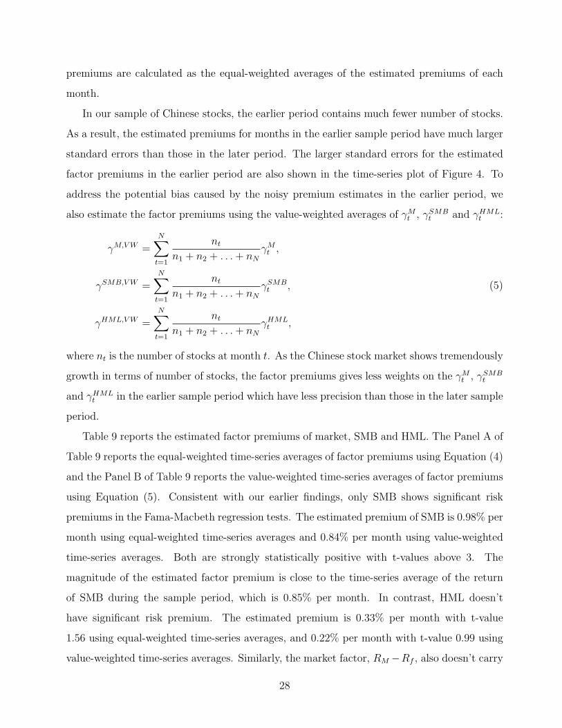
Table 9 reports the estimated factor premiums of market, SMB and HML. The Panel A of

Table 9 reports the equal-weighted time-series averages of factor premiums using Equation (4)

and the Panel B of Table 9 reports the value-weighted time-series averages of factor premiums

using Equation (5). Consistent with our earlier findings, only SMB shows significant risk

premiums in the Fama-Macbeth regression tests. The estimated premium of SMB is 0.98% per

month using equal-weighted time-series averages and 0.84% per month using value-weighted

time-series averages. Both are strongly statistically positive with t-values above 3. The

magnitude of the estimated factor premium is close to the time-series average of the return

of SMB during the sample period, which is 0.85% per month. In contrast, HML doesn’t

have significant risk premium. The estimated premium is 0.33% per month with t-value

1.56 using equal-weighted time-series averages, and 0.22% per month with t-value 0.99 using

value-weighted time-series averages. Similarly, the market factor, RM −Rf , also doesn’t carry

28

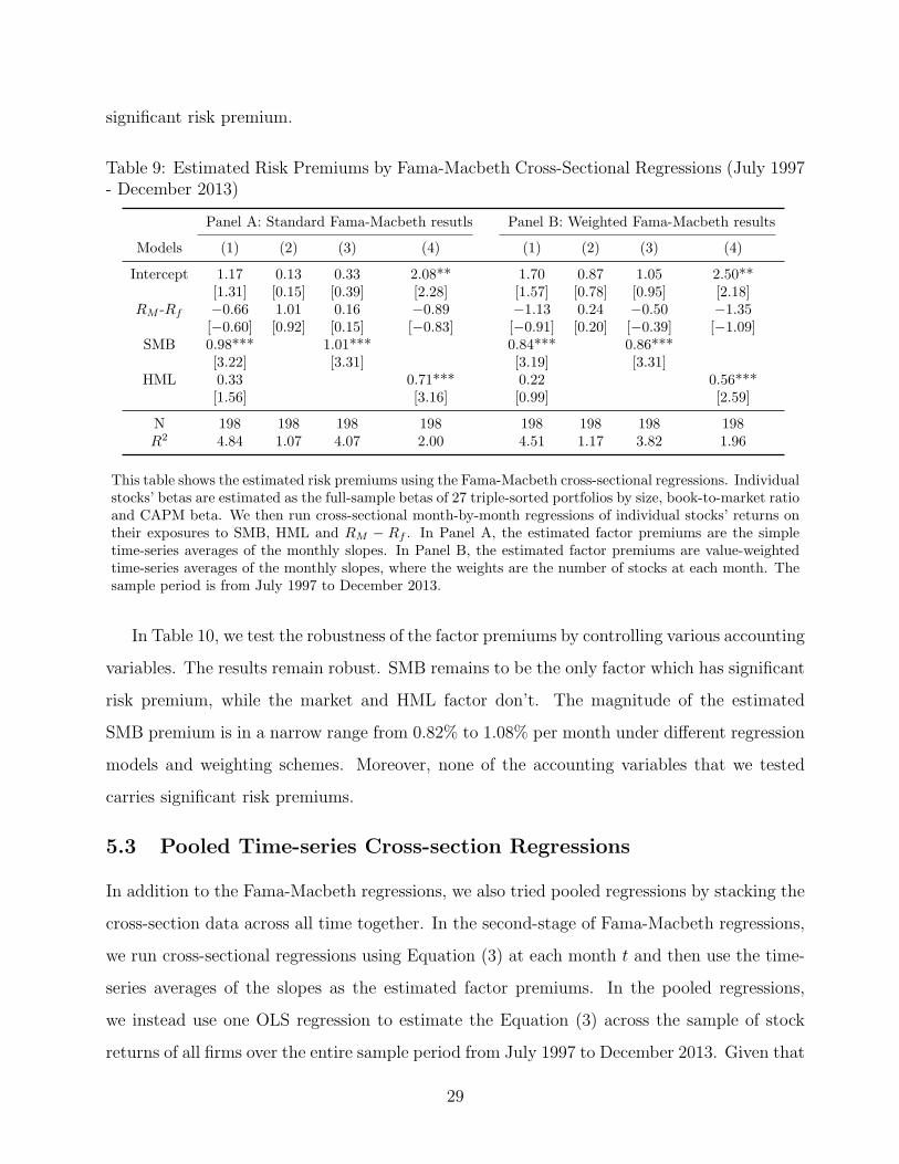
significant risk premium.

Table 9: Estimated Risk Premiums by Fama-Macbeth Cross-Sectional Regressions (July 1997- December 2013)

Panel A: Standard Fama-Macbeth resutls Panel B: Weighted Fama-Macbeth results

Models (1) (2) (3) (4) (1) (2) (3) (4)

Intercept 1.17 0.13 0.33 2.08** 1.70 0.87 1.05 2.50**[1.31] [0.15] [0.39] [2.28] [1.57] [0.78] [0.95] [2.18]

RM -Rf −0.66 1.01 0.16 −0.89 −1.13 0.24 −0.50 −1.35[−0.60] [0.92] [0.15] [−0.83] [−0.91] [0.20] [−0.39] [−1.09]

SMB 0.98*** 1.01*** 0.84*** 0.86***[3.22] [3.31] [3.19] [3.31]

HML 0.33 0.71*** 0.22 0.56***[1.56] [3.16] [0.99] [2.59]

N 198 198 198 198 198 198 198 198R2 4.84 1.07 4.07 2.00 4.51 1.17 3.82 1.96

This table shows the estimated risk premiums using the Fama-Macbeth cross-sectional regressions. Individualstocks’ betas are estimated as the full-sample betas of 27 triple-sorted portfolios by size, book-to-market ratioand CAPM beta. We then run cross-sectional month-by-month regressions of individual stocks’ returns ontheir exposures to SMB, HML and RM − Rf . In Panel A, the estimated factor premiums are the simpletime-series averages of the monthly slopes. In Panel B, the estimated factor premiums are value-weightedtime-series averages of the monthly slopes, where the weights are the number of stocks at each month. Thesample period is from July 1997 to December 2013.

In Table 10, we test the robustness of the factor premiums by controlling various accounting

variables. The results remain robust. SMB remains to be the only factor which has significant

risk premium, while the market and HML factor don’t. The magnitude of the estimated

SMB premium is in a narrow range from 0.82% to 1.08% per month under different regression

models and weighting schemes. Moreover, none of the accounting variables that we tested

carries significant risk premiums.

5.3 Pooled Time-series Cross-section Regressions

In addition to the Fama-Macbeth regressions, we also tried pooled regressions by stacking the

cross-section data across all time together. In the second-stage of Fama-Macbeth regressions,

we run cross-sectional regressions using Equation (3) at each month t and then use the time-

series averages of the slopes as the estimated factor premiums. In the pooled regressions,

we instead use one OLS regression to estimate the Equation (3) across the sample of stock

returns of all firms over the entire sample period from July 1997 to December 2013. Given that

29

Table 10: Fama-Macbeth Regressions with Accounting Variables Controls (July 1997 - De-cember 2013)

Models Intercept RM −Rf SMB HML Floating A/BE A/ME E/P dummy E(+)/P D/P N R2

Panel A: Standard Fama-Macbeth regressions

1 1.17 −0.66 0.98*** 0.33 198 4.84[1.31] [−0.60] [3.22] [1.56]

2 1.21 −0.91 1.06*** 0.33 0.46 198 5.43[1.31] [−0.83] [3.11] [1.55] [0.96]

3 1.16 −0.59 0.99*** 0.20 0.14 198 5.20[1.29] [−0.54] [3.23] [1.07] [1.22]

4 1.28 −0.46 1.02*** 0.31** −0.25 198 5.57[1.43] [−0.44] [3.46] [2.22] [−1.49]

5 0.78 −0.39 1.08*** 0.24 −0.08 0.04 198 6.69[0.82] [−0.36] [4.30] [1.17] [−0.42] [0.86]

6 0.94 −0.49 1.02*** 0.29 0.06 198 5.20[1.05] [−0.46] [3.47] [1.36] [1.50]

Panel B: Weighted Fama-Macbeth regressions

1 1.70 −1.13 0.84*** 0.22 198 4.51[1.57] [−0.91] [3.19] [0.99]

2 1.70 −1.15 0.85*** 0.24 −0.03 198 4.98[1.50] [−0.93] [3.08] [1.05] [−0.08]

3 1.70 −1.10 0.82*** 0.18 0.07 198 4.86[1.55] [−0.87] [3.20] [0.88] [0.55]

4 1.76 −0.95 0.86*** 0.21* −0.23 198 5.15[1.63] [−0.80] [3.50] [1.69] [−1.37]

5 1.20 −0.79 0.96*** 0.14 −0.17 0.04 198 6.14[1.07] [−0.63] [4.39] [0.69] [−0.81] [1.14]

6 1.44 −0.95 0.88*** 0.17 0.07* 198 4.84[1.34] [−0.77] [3.47] [0.79] [1.85]

This table shows the estimated risk premiums using the Fama-Macbeth cross-sectional regressions. Individualstocks’ betas are estimated as the full-sample betas of 27 triple-sorted portfolios by size, book-to-market ratioand CAPM beta. We then run cross-sectional month-by-month regressions of individual stocks’ returns ontheir exposures to SMB, HML and RM −Rf ,and accounting variables as controlling variables. In Panel A,the estimated factor premiums are the simple time-series averages of the monthly slopes. In Panel B, theestimated factor premiums are value-weighted time-series averages of the monthly slopes, where the weightsare the number of stocks at each month. The sample period is from July 1997 to December 2013.

the error terms are likely to be cross-sectional correlated at a given month, we clustered the

standard-errors at the month level. The pooled regression and the Fama-Macbeth regressions

are indeed two similar approaches. Cochrane (2005) has shown that under certain technical

conditions, the two approaches will have identical numerical results. Nevertheless, given that

the Chinese stock market had few stocks and was more volatile in the early period, we think

it is helpful to report the pooled time-series cross-section regression results as a robustness

check.

Table 11 reports the estimated premiums and the adjusted t-statistics for the pooled

30

regressions. The results are similar to the ones using the Fama-Macbeth approach. SMB

has a robust positive risk premium of 0.78% per month, while the other two factors, market

and HML, don’t have significant premiums and are thus not priced on average in the Chinese

market. In addition, the size factor significantly improves the R2 of the pooled regressions.

The R2 for the pooled regression with only the market factor is less than 0.01%. Adding HML

together with the market factor improves the R2 only marginally. In contrast, when the size

factor SMB is included, the R2 increases to 0.07%, confirming the strong explanatory power

of SMB in explaining the cross-section returns.

Table 11: Estimated Risk Premiums by Pooled Regressions (July 1997 - December 2013)

Models (1) (2) (3) (4)

Intercept 1.77* 1.16 1.13 2.38**[ 1.79] [ 1.05] [ 1.03] [ 2.35]

RM -Rf −1.16 −0.02 −0.56 −1.22[−0.98] [−0.02] [−0.47] [−1.04]

SMB 0.78*** 0.82***[ 2.75] [ 2.92]

HML 0.20 0.41[ 0.80] [ 1.60]

N 185316 185316 185316 185316R2 0.07 0.00 0.06 0.01

Individual stocks’ exposures to SMB, HML and RM − Rf are first estimated as the full-sample betas of27 triple-sorted portfolios by size, book-to-market ratio and CAPM beta. Next, the equation, Ri

t − Rf,t =γ0,t+γM

t βMi +γSMB

t βSMBi +γHML

t βHMLi +ϵit, is estimated in one single OLS regression by pooling individual

stock returns across all months together. T-statistics are estimated based on standard errors clustered bymonth. The sample period is from July 1997 to December 2013.

6 Robustness

6.1 Sample Period from July 1995 to December 2013

Our main results can be summarized as 1) strong size effect - smaller firms, on average, have

higher returns than bigger firms; and 2) no value effect - value and growth firms don’t have

significant different returns. Our findings contradict some of the existing literature on the

Chinese stock market, including Chen, Kim, Yao, and Yu (2010), Nusret Cakici and Topyan

(2011) and Carpenter, Lu, and Whitelaw (2014), where they find strong size and value effect.

31

The disagreement stems mainly from different choices of sample periods. We use the returns

of Chinese firms listed on the Shanghai and Shenzhen exchanges from July 1997 to December

2013 for the asset pricing tests; Chen, Kim, Yao, and Yu (2010) use data from July 1995

to June 2007; Nusret Cakici and Topyan (2011) use data from January 1994 to March 2011;

Carpenter, Lu, and Whitelaw (2014) use data from July 1995 to December 2012. In fact,

the major difference lies in whether the period predates July 1997. We test the robustness of

our results by expanding our sample period to cover 222 months from July 1995 to December

2013, which is longer than all samples used in the existing literature of which we are aware.

The Panel A and Panel B of Table 12 report the Fama-Macbeth regression results based

on the sample from July 1995 to December 2013. Panel A reports the equal-weighted average

premiums and Panel B reports the value-weighted average premiums. In both panels, SMB

remains to be the only factor that carries a significant factor premium with t-value above

2.60. The estimated premium for HML remains to be not statistically significant at the 5%

confidence level. However, the t-values are close to marginal significant. The t-value of HML

factor premium is 1.69 for the equal-weighting scheme in Panel A and 1.22 for the value-

weighting scheme in Panel B.

In the pooled regression tests, Table 13 shows that the HML premium is estimated to be

0.32% with t-value 1.76 which is marginally significant.

Figure 4 plots the estimated slopes of the Fama-Macbeth regressions, γSMB and γHML,

month-by-month from July 1995 to December 2013. It is clear that the estimated slopes

are much noisier from 1995 to 1997, when compared with later periods. After July 1997,

all of the estimated slopes on HML are within the range from −10% to +10%. In contrast,

the estimated slopes during the 24 months from July 1995 to June 1997 appear to be much

noisier. There are five months when the slopes are outside of the [−10%, 10%] band during

the 24 months from July 1995 to June 1997. On two months, July 1996 and October 1996,

the estimated slopes are even above 35%. Given that there are only 222 months from July

1995 to December 2013, the extreme values of the estimated slopes in the first two years might

have a heavy impact on the factor premiums.

To address this concern, we test the robustness of the estimated premiums by excluding

the two months, July 1996 and October 1996, from our extended sample from July 1995

32

Table 12: Estimated Risk Premiums by Fama-Macbeth Cross-Sectional Regressions (July1995 - December 2013)

Monthly observations from July 1995 to December 2013Panel A: Standard Fama-Macbeth regressions Panel B: Weighted Fama-Macbeth regressions

Models (1) (2) (3) (4) (1) (2) (3) (4)

Intercept −0.41 −3.07** −2.01 −0.51 0.46 −1.04 0.12 0.33[−0.43] [−2.15] [−1.37] [−0.53] [0.46] [−1.09] [0.12] [0.33]

RM -Rf 1.32 4.34*** 2.90* 1.84 0.17 2.14** 0.51 0.81[1.22] [2.83] [1.78] [1.62] [0.13] [2.16] [0.46] [0.64]

SMB 0.83*** 0.86*** 0.87*** 0.86***[2.68] [2.96] [3.35] [3.57]

HML 0.65* 0.87** 0.22 0.45***[1.69] [2.30] [1.22] [2.63]

N 222 222 222 222 222 222 222 222R2 5.35 1.41 4.21 2.45 4.20 1.02 3.45 1.67

Monthly observations from July 1995 to December 2013Excluding July 1996 and Octor 1996

Panel C: Standard Fama-Macbeth regressions Panel D: Weighted Fama-Macbeth regressions

Models (1) (2) (3) (4) (1) (2) (3) (4)

Intercept −0.87 −1.93* −0.88 −0.98 0.34 −0.73 0.42 0.21[−0.98] [−1.94] [−0.85] [−1.08] [0.34] [−0.80] [0.42] [0.21]

RM -Rf 1.61 3.05*** 1.65 2.12* 0.24 1.80* 0.18 0.88[1.44] [3.01] [1.47] [1.83] [0.19] [1.88] [0.17] [0.69]

SMB 0.76** 0.73** 0.85*** 0.83***[2.37] [2.47] [3.25] [3.38]

HML 0.29 0.51*** 0.12 0.35**[1.39] [2.58] [0.79] [2.34]

N 220 220 220 220 220 220 220 220R2 5.12 1.31 4.11 2.20 4.13 0.99 3.43 1.61

This table shows the estimated risk premiums using the Fama-Macbeth cross-sectional regressions. Individualstocks’ exposures to SMB, HML and RM − Rf are estimated as the full-sample betas of 27 triple-sortedportfolios by size, book-to-market ratio and CAPM beta. We then run cross-sectional month-by-monthregressions of individual stocks’ returns on their betas. In Panel A and Panel C, the estimated factorpremiums are the simple time-series averages of the monthly slopes. In Panel B and Panel D, the estimatedfactor premiums are value-weighted time-series averages of the monthly slopes, where the weights are thenumber of stocks at each month. The sample period for Panel A and Panel B is 222 months from July1995 to December 2013, and the sample period for Panel B and Panel D is 220 months from July 1995 toDecember 2013 but excluding July 1996 and October 1996.

to December 2013. Panel C and Panel D of Table 12 shows that the t-values of the factor

premiums associated with HML drop significantly after the two months are excluded from

the sample. The t-value of the estimated premium of HML drops to 1.39 when using equal-

weighted averages and 0.79 when using value-weighted averages. Similarly, in the pooled

33

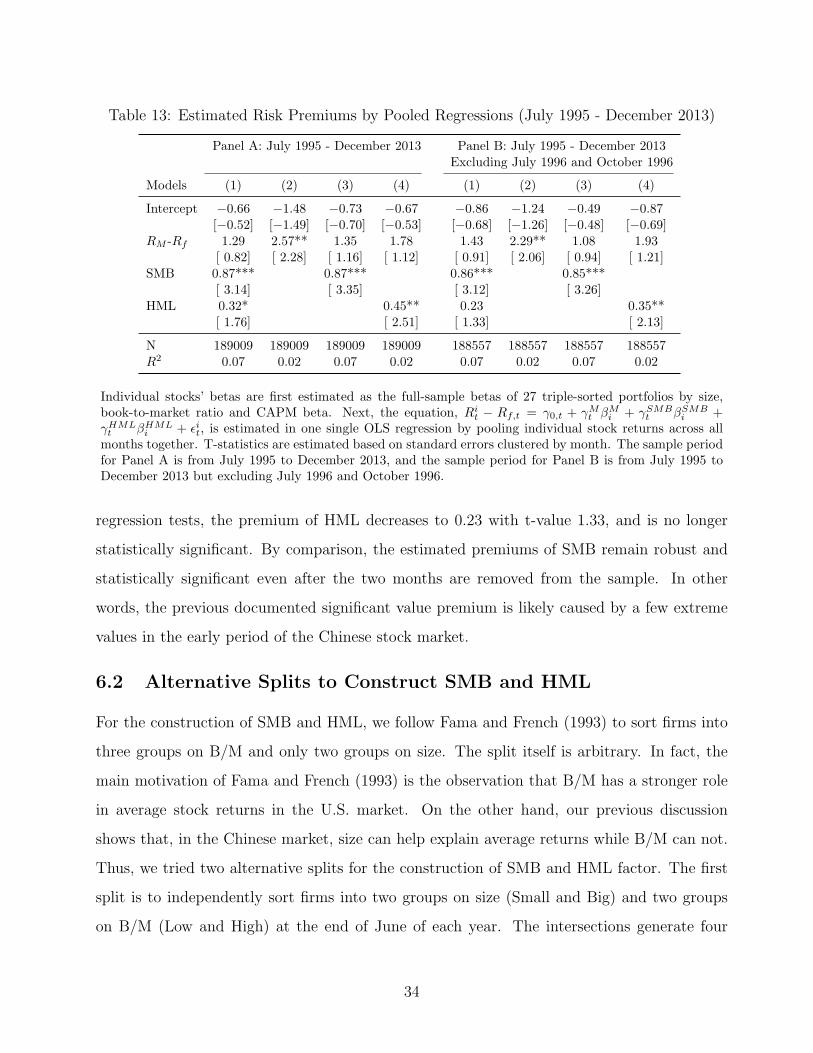
Table 13: Estimated Risk Premiums by Pooled Regressions (July 1995 - December 2013)

Panel A: July 1995 - December 2013 Panel B: July 1995 - December 2013Excluding July 1996 and October 1996

Models (1) (2) (3) (4) (1) (2) (3) (4)

Intercept −0.66 −1.48 −0.73 −0.67 −0.86 −1.24 −0.49 −0.87[−0.52] [−1.49] [−0.70] [−0.53] [−0.68] [−1.26] [−0.48] [−0.69]

RM -Rf 1.29 2.57** 1.35 1.78 1.43 2.29** 1.08 1.93[ 0.82] [ 2.28] [ 1.16] [ 1.12] [ 0.91] [ 2.06] [ 0.94] [ 1.21]

SMB 0.87*** 0.87*** 0.86*** 0.85***[ 3.14] [ 3.35] [ 3.12] [ 3.26]

HML 0.32* 0.45** 0.23 0.35**[ 1.76] [ 2.51] [ 1.33] [ 2.13]

N 189009 189009 189009 189009 188557 188557 188557 188557R2 0.07 0.02 0.07 0.02 0.07 0.02 0.07 0.02

Individual stocks’ betas are first estimated as the full-sample betas of 27 triple-sorted portfolios by size,book-to-market ratio and CAPM beta. Next, the equation, Ri

t − Rf,t = γ0,t + γMt βM

i + γSMBt βSMB

i +γHMLt βHML

i + ϵit, is estimated in one single OLS regression by pooling individual stock returns across allmonths together. T-statistics are estimated based on standard errors clustered by month. The sample periodfor Panel A is from July 1995 to December 2013, and the sample period for Panel B is from July 1995 toDecember 2013 but excluding July 1996 and October 1996.

regression tests, the premium of HML decreases to 0.23 with t-value 1.33, and is no longer

statistically significant. By comparison, the estimated premiums of SMB remain robust and

statistically significant even after the two months are removed from the sample. In other

words, the previous documented significant value premium is likely caused by a few extreme

values in the early period of the Chinese stock market.

6.2 Alternative Splits to Construct SMB and HML

For the construction of SMB and HML, we follow Fama and French (1993) to sort firms into

three groups on B/M and only two groups on size. The split itself is arbitrary. In fact, the

main motivation of Fama and French (1993) is the observation that B/M has a stronger role

in average stock returns in the U.S. market. On the other hand, our previous discussion

shows that, in the Chinese market, size can help explain average returns while B/M can not.

Thus, we tried two alternative splits for the construction of SMB and HML factor. The first

split is to independently sort firms into two groups on size (Small and Big) and two groups

on B/M (Low and High) at the end of June of each year. The intersections generate four

34

portfolios: Small-Low, Small-High, Big-Low and Big-High. The monthly returns of the four

portfolios are the value-weighted average of individual stock returns, in which the weights are

floating A-share market capitalizations at the portfolio formation time. SMB is the difference

between the simple average of the returns on the two small-stock portfolios (Small-Low and

Small-High) and the two big-stock portfolio (Big-Low and Big-High).

The second split is similar, except that we sort firms into three groups on size (Small,

Medium and Big) and two groups on B/M (Low and High). The three size portfolios repre-

sent the bottom 30%, middle 40% and top 30% of stocks ranked on the basis of size. The

intersections generate six portfolios: Small-Low, Small-High, Medium-Low, Medium-High,

Big-Low and Big-High. SMB is the difference between the simple average of the returns on

the two small-stock portfolios (Small-Low and Small-High) and the two big-stock portfolio

(Big-Low and Big-High).

Table 14 summarizes the Fama-Macbeth results for the above 2-by-2 and 3-by-2 splits.

The results confirm the robust positive premium of the size factor. The average premiums

for SMB are of similar magnitude as our main results, and remain positively significant. The

average premiums for HML are still positive, but non-significant. Our main conclusions are

thus robust to different splits in the construction of size and value factors.

6.3 Alternative Definition of Size

Due to the “split-share structure”, Chinese-listed firms often have both floating shares and

non-floating shares. In the main part of this paper, we define a firm’s size as the floating A-

share market capitalization because regular investors can only publicly trade floating A shares.

However, some papers do use the total market capitalization to define size. To compare our

results with them on an equal footing, we test the robustness of our main results for different

measures of size.

Definition of size affects the construction of RM−Rf , SMB and HML factors in two dimen-

sions. First, it determines individual stocks’ ranking when we form two size portfolios: Small

and Big. Second, the relative weights for individual stocks within a portfolio, e.g. market,

Small-Low, Small-Medium, Small-High, Big-Low, Big-Medium and Big-High, are determined

by their size. Hence, we have in total six combinations: rank by floating capitalization and

35

Table 14: Alternative Splits to Construct SMB and HML

Panel A: Two size-sorted portfolios and two B/M sorted portfolios

RM −Rf SMB HML N R2

1 −0.50 [−0.39] 0.87*** [3.31] 198 3.822 −1.49 [−1.20] 0.44*** [2.72] 198 1.973 −1.18 [−0.95] 0.84*** [3.16] 0.18 [1.06] 198 4.51

Panel B: Three size-sorted portfolios and two B/M sorted portfolios

RM −Rf SMB HML N R2

1 −0.46 [−0.36] 1.13*** [3.33] 198 3.832 −1.44 [−1.16] 0.40*** [2.65] 198 1.973 −1.14 [−0.91] 1.10*** [3.20] 0.16 [1.03] 198 4.52

Value-weighted Fama-Macbeth regression results are reported for different splits to construct SMB and HMLfactors. The weights are the number of observations at each month, and the sample period is from July 1997to December 2013. In panel A, stocks are sorted on the basis of size into two groups (Small and Big) and twogroups on B/M ratios (Low and High) at the end of June of each year from 1997 to 2013. The intersectionsgenerate four portfolios: Small-Low, Small-High, Big-Low and Big-High. SMB is the difference between thesimple average of the returns on the two small-stock portfolios (Small-Low and Small-High) and the twobig-stock portfolios (Big-Low and Big-High). In panel B, stocks are sorted into three groups on size (Small,Medium and Big) and two groups on B/M (Low and High). The three size groups represent the bottom30%, middle 40% and top 30% of stocks ranked on the basis of size. The intersections generate six portfolios:Small-Low, Small-High, Medium-Low, Medium-High, Big-Low and Big-High. SMB is the difference betweenthe simple average of the returns on the two small-stock portfolios (Small-Low and Small-High) and the twobig-stock portfolio (Big-Low and Big-High).

weight by floating capitalization, rank by floating and weight by total, rank by floating and

weight equally, rank by total and weight by floating, rank by total and weight by total and

rank by total and weight equally.

The Fama-Macbeth results for the above six cases are summarized in Table 15. Different

ranking and weighting schemes produce similar RM −Rf , SMB and HML factors. The time-

series average and t-values for the returns on the three factors show very small differences.

Not surprisingly, the estimated risk premiums in the Fama-Macbeth regressions are also close.

SMB has a robust positive premium and RM −Rf and HML don’t.

7 Conclusions

We find stock returns are strongly related to firms’ size in the Chinese market. On average,

small stocks outperform large stocks. The average returns on stocks in the smallest size

36

Table 15: Alternative Definition of Size

Sorted by floating cap Sorted by total cap

Weighted by Floating Total Equal Floating Total Equal

Panel A: Summary statistics of Fama-French 3 factors

RM -Rf 0.60 0.47 1.12 0.60 0.47 1.12[0.97] [0.80] [1.66] [0.97] [0.80] [1.66]

SMB 0.85*** 0.85*** 0.76*** 0.85*** 0.86*** 0.81***[3.09] [3.08] [3.63] [3.08] [3.09] [3.94]

HML 0.34 0.36 0.33* 0.29 0.30 0.28[1.61] [1.68] [1.75] [1.40] [1.43] [1.47]

Panel B: Fama-Macbeth regression results on the loadings of 3 factors

Intercept 1.70 1.72 1.74 1.70 1.92* 2.10*[1.57] [1.59] [1.57] [1.54] [1.70] [1.82]

RM -Rf −1.13 −1.15 −1.17 −1.31 −0.84 −1.00[−0.91] [−0.93] [−0.92] [−1.03] [−0.62] [−0.74]

SMB 0.84*** 0.85*** 0.68*** 0.87*** 0.84*** 0.67***[3.19] [3.17] [3.47] [3.25] [3.10] [3.52]

HML 0.22 0.23 0.15 0.14 0.16 0.10[0.99] [1.01] [0.78] [0.65] [0.71] [0.51]

N 198 198 198 198 198 198R2 4.51 4.51 4.52 4.50 4.51 4.52

Definition of size affects the construction of RM −Rf , SMB and HML factors in two dimensions: individualstocks’ rank in size and their relative weights in a portfolio. Six different methods are examined: rank byfloating capitalization and weight by floating capitalization, rank by floating and weight by total, rank byfloating and weight equally, rank by total and weight by floating, rank by total and weight by total andrank by total and weight equally. Panel A reports the time-series summary statistics of RM − Rf , SMBand HML for each method. Panel B reports the risk premiums estimated by value-weighted Fama-Macbethregressions. The weights are the number of observations at each month, and the sample period is from July1997 to December 2013.

decile is 1.63% higher than those in the largest size decile. Following the classic Fama-French

methodology, we construct a zero-cost portfolio, small-minus-big (SMB), to mimic the strong

size effect in the cross-section returns. SMB earns an average monthly returns of 0.85%, not

only economically large but also statistically significant. In contrast, stocks’ average returns

don’t exhibit clear relation with their book-to-market ratios. The factor mimicking portfolio

for the book-to-market ratios, high-minus-low (HML), generates an average monthly returns

of 0.34%, positive but not statistically significant. The market factor, RM −Rf , also doesn’t

have significant premium. Moreover, SMB consistently beats the market and HML factors

in both time-series regressions and Fama-Macbeth cross-sectional tests. Among the three

37

factors, SMB is the most important one in terms of capturing cross-sectional variations in

Chinese stock returns.

Our results contradict some previous literature which documented strong size and value

effect. The differences stem mainly from choices of sample periods. Our results are based on

a relative stable period from July 1997 to December 2013, while other papers usually include

earlier years from 1995 to 1996. In the robustness check, we find that the previous documented

value effect is not robust and is largely caused by a few extreme months before 1997.

38

References

Agarwalla, S. K., J. Jacob, and J. R. Varma (2013). Four Factor Model in Indian Equities

Market. Working Paper, Indian Institute of Management Ahmedabad.

Banz, R. W. (1981). The Relationship between Return and Market Value of Common

Stocks. Journal of Financial Economics 9 (1), 3–18.

Basu, S. (1983). The Relationship between Earnings’ Yield, Market Value and Return for

NYSE Common Stocks: Further Evidence. Journal of Financial Economics 12 (1), 129–

156.

Bruckner, R., P. Lehmann, M. H. Schmidt, and R. Stehle (2014). Fama-French Factors for

Germany: Which Set is Best? Working Paper, Humboldt University.

Carpenter, J. N., F. Lu, and R. F. Whitelaw (2014). The Real Value of Chinas Stock

Market. Working Paper, New York University.

Chan, K., A. J. Menkveld, and Z. Yang (2008). Information Asymmetry and Asset Prices:

Evidence from the China Foreign Share Discount. Journal of Finance 63 (1), 159–196.

Chan, L. K. C., Y. Hamao, and J. Lakonishok (1991). Fundamentals and Stock Returns in

Japan. The Journal of Finance 46 (5), 1739–1764.

Chen, X., K. A. Kim, T. Yao, and T. Yu (2010). On the Predictability of Chinese Stock

Returns. Pacific-Basin Finance Journal 18 (4), 403–425.

Chou, P.-H., K.-C. Ko, S.-T. Kuo, and S.-J. Lin (2012). Firm Characteristics, Alter-

native Factors, and Asset-Pricing Anomalies: Evidence from Japan. Quantitative Fi-

nance 12 (3), 369–382.

Cochrane, J. H. (2005). Asset Pricing. Princeton University Press.

Cordeiro, R. and M. Machado (2013). Value or Growth Strategy? Empirical Evidence in

Brazil. Review of Business Management 15 (46), 91–111.

Docherty, P., H. Chan, and S. Easton (2013). Australian Evidence on the Implementation

of the Size and Value Premia. Accounting & Finance 53 (2), 367–391.

39

Drew, M. E. and M. Veeraraghavan (2002). A Closer Look at the Size and Value Premium in

Emerging Markets: Evidence from the Kuala Lumpur Stock Exchange. Asian Economic

Journal 16 (4), 337–351.

Fama, E. and K. R. French (1992). The Cross-Section of Expected Stock Returns. The

Journal of Finance 47 (2), 427–465.

Fama, E. and K. R. French (1993). Common Risk Factors in the Returns on Stocks and

Bonds. Journal of Financial Economics 33 (1), 3–56.

Fama, E. and K. R. French (2012). Size, Value, and Momentum in International Stock

Returns. Journal of Financial Economics 105 (3), 457–472.

Fama, E. and J. D. MacBeth (1973). Risk, Return, and Equilibrium: Empirical Tests.

Journal of Political Economy 81 (3), 607–636.

Jensen, M. C., F. Black, and M. S. Scholes (1972). The Capital Asset Pricing Model: Some

Empirical Tests. Michael C. Jensen. Studies in the Theory of Capital Markets 81 (3),

79–121.

Mei, J., J. A. Scheinkman, and W. Xiong (2009). Speculative Trading and Stock Prices:

Evidence from Chinese A-B Share Premia. Annals of Economics and Finance 10 (2),

225–255.

Michou, M., S. Mouselli, and A. W. Stark (2013). Fundamental Analysis and the Modelling

of Normal Returns in the UK . Working Paper, University of Edinburgh Business School

and University of Manchester.

Moerman, G. A. (2005). How Domestic is the Fama and French Three-Factor Model? An

Application to the Euro Area. Working Paper, Erasmus Research Institute of Manage-

ment.

Nartea, G. V., C. Gan, and J. G. Wu (2008). Persistence of Size and Value Premia and the

Robustness of the Fama-French Three Factor Model in the Hong Kong Stock Market.

Investment management and Financial Innovations 5 (4), 39–49.

Nusret Cakici, K. C. and K. Topyan (2011). Cross-Sectional Stock Return Predictability

in China. Working Paper, Fordham University, Hong Kong University of Science and

40

Technology and Manhattan College.

Stattman, D. (1980). Book Values and Stock Returns. The Chicago MBA: A journal of

selected papers 4 (1), 25–45.

Veltri, S. and A. Silvestri (2011). Direct and Indirect Effects of Human Capital on Firm

Value: Evidence from Italian Companies. Journal of Human Resource Costing & Ac-

counting 15, 232–254.

Wang, F. and Y. Xu (2004). What Determines Chinese Stock Returns? Financial Analysts

Journal 60 (6), 65–77.

Wang, J., X. Hu, and J. Pan (2014). 2013 Chinese Capital Market Yearbook.

41