Farm MachineryOperation CostCalculations

Terry KastensExtension Agricultural Economist

Kansas State University

Kansas State University Agricultural Experiment Station and Cooperative Extension Service

1

Valuing Machinery Over Time 4

Analysis Time Period 4

Current List Price 4

Producer Price Index 4

Remaining Value Percentage,Economic Depreciation, andMarket Value 6

Purchase Price and Selling Price 10

Annual Operating Costs 11

Field Efficiency 11

Fuel and Lubrication 11

Labor 11

Repair and Maintenance 13

Timeliness 15

Property Taxes, Insurance, and Shelter 16

Income Tax and Finance 16

Marginal Tax Rates 16

Cost of Capital 16

Net Present Value 17

Amortized Annual Cash Flow 18

Finance 18

Income Tax Depreciation 2 0

Income Tax Savings 21

Net Cash Inflows for ComputingNet Present Value 21

Using the Machinery CostAnalysis Results to Make Decisions 21

Example 1: Costs for a NewCase-IH Combine across ThreeUsage Rates 22

Example 2: Costs for a NewCase-IH Combine across ThreeInflation Rates 22

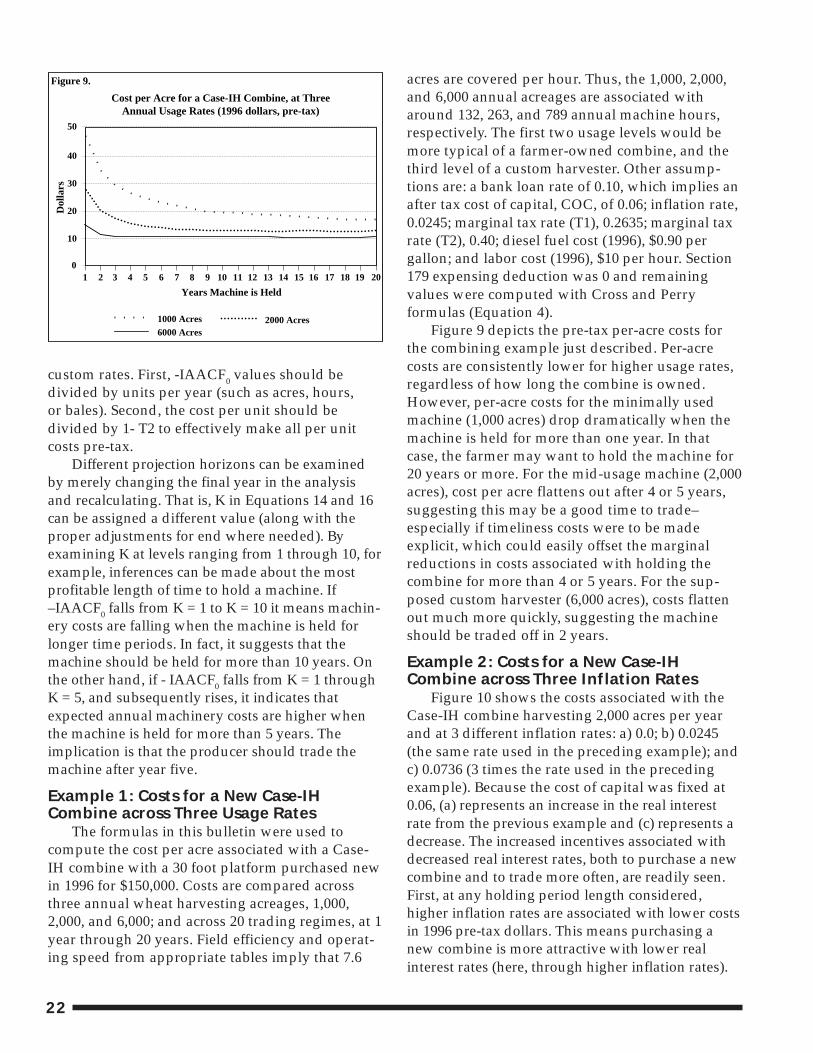
Example 3: Costs for a New 8-RowPlanter with and without Section179 Expensing Deduction 23

Conclusion 23

References 23

Tables

Table 1. Producer Price Index,U.S. Average, All Commodities 5

Table 2. Factors for CalculatingRemaining Value Percentagesby Machinery Class 6

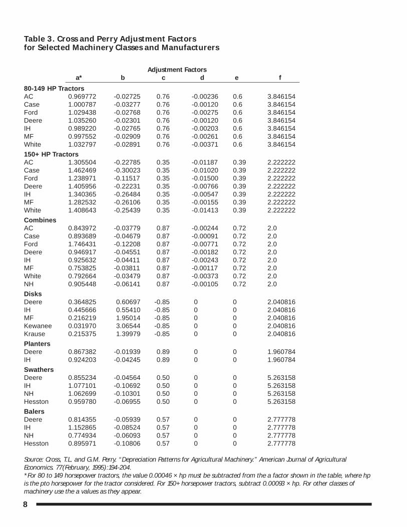
Table 3. Cross and Perry AdjustmentFactors for Selected Machinery Classesand Manufacturers 8

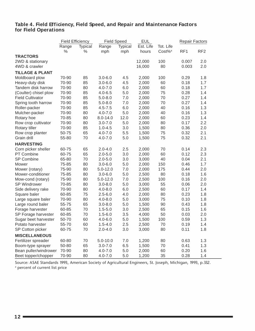
Table 4. Field Efficiency, Field Speed,and Repair and Maintenance Factorsfor Field Operations 12

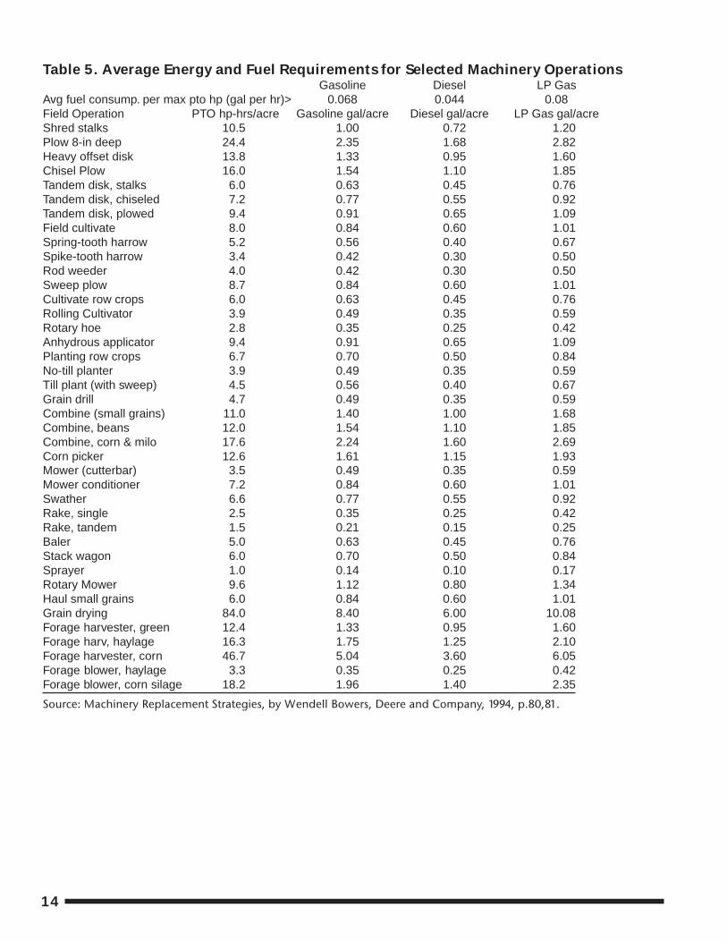
Table 5. Average Energy and FuelRequirements for Selected MachineryOperations 14

Figures

Figure 1. Annual Inflation Based onProducer Price Index, 1950-1996 5

Figure 2. Remaining Value as a Percentof Current List Price by Age, for SeveralMachinery Classes 7

Figure 3. Remaining Value as a Percentof Current List Price for Combines withAnnual Usage of 200 Hours 9

Figure 4. Annual Depreciation as a Percentof Previous Year’s Price for Combines withAnnual Usage of 200 Hours 9

Figure 5. Remaining Value as a Percentof Current List Price for a Deere Combineacross Various Annual Usage Rates 9

Figure 6. Remaining Value as a Percentof Current List Price for 175 hp Tractorswith Annual Usage of 500 Hours 10

Figure 7. Annual Depreciation as aPercent of Last Year’s Price for 175 hpTractors with Annual Usage of 500 Hours 10

Figure 8. Accumulated Repairs as aPercent of Current List Price for a TandemDisk across Three Annual Usage Rates 13

Figure 9. Cost per Acre for a Case-IHCombine, at Three Annual Usage Rates 22

Figure 10. Cost per Acre for a Case-IHCombine at Three Annual Inflation Rates 23

Figure 11. Cost per Acre for an 8-Row Planter,with and without Section 179 Deduction 23

Contents

2

Abbreviations Used in this PublicationAC Allis Chalmers GleanerAGE Machine’s age in yearsAH Accumulated Hours on a MachineAPH Acres per HourARM Accumulated Repair and Maintenance ChargesASAE American Society of Agricultural EngineersBTBASIS Beginning Tax Basis at the Time of PurchaseCF Cash FlowCLP Current List PriceCOC Cost of Capital Ratedep1, dep2 Depreciation FactorsDFCF Tax Deductable Financing Cash FlowEUL Estimated Useful LifeFEP Field Efficiency PercentageFL Fuel and Lubrication ChargesFS Field SpeedGAIN Selling Price Less Tax BasisHPY Average Hours per Year of machine usage since it was newIAACF Inflation Adjusted Amortized Annual Cash FlowIH International HarvesterITS Income Tax SavingsLAB Annual Labor ChargesMACRS Modified Accelerated Cost Recovery SystemMF Massey FergusonMV Market ValueMW Machine WidthNDFCF Nondeductible Financing Cash FlowNH New HollandNPV Net Present ValuePPI Producer Price IndexPUR Purchase PriceRAF Repair Adjustment FactorRF1, RF2 Repair FactorsRM Repair and Maintenance Charge for a Specific YearRVP Remaining Value PercentageSE Net Self-employment Tax RateSEC179 Section 179 Expense DeductionSELL Selling PriceT1 Federal and State Income Tax RateT2 Federal and State Income Tax Rate, Including Self-employment Tax RateTBASIS Remaining Tax Basis in any Given YearTDEPR Tax Depreciation in a Given YearTIS Property Taxes, Insurance, and Shelter

3

Machinery operating and ownership costs areoften more than half of total crop production costsfor Kansas producers and substantially affect farmprofitability. Besides affecting fundamental ma-chinery buying and trading decisions, machinerycosts affect profit-maximizing crop and rotationselection, thus long-run farm profitability. Under-standing machinery costs becomes especiallycrucial when considering alternative croppingsystems, particularly when less tillage is involved.In short, machinery costs enter farm managementin three areas: 1) minimizing costs of production,2) selecting the profit-maximizing crop mix, and3) considering structural or technological changes,such as farm expansion or contraction, or alterna-tive tillage systems.

Minimizing the machinery portion of produc-tion costs requires routine assessment of the ben-efits and costs associated with owning, leasing, orrenting machinery. These must regularly be com-pared with hiring machinery operations (customfarming), which is often a plausible alternative. Toassist farm managers in machinery decisions, thisbulletin develops a framework for calculating andanalyzing the various components of a machine’sexpected annual costs: repairs and maintenance;gas, fuel, and oil; operating labor; insurance andtaxes; depreciation; and opportunity cost on fundsused.

For crop enterprise selection, machinery costsmust be assigned to specific crops or crop se-quences. Actual historical machine costs canprovide a basis for such assignments but may bedifficult to obtain. That is, some costs associatedwith machinery operations are difficult to allocateto the usage of specific machines. However, be-cause producers can identify each machine and thenumber of its operations associated with a crop, aframework for calculating a machine’s expectedcosts can assist in developing crop-specific machin-ery costs.

Machinery costs are especially important whenconsidering structural or technological changes.For example, recently acquired rented land, requir-ing additional machinery, may be unavailable inthe future. An experiment in no-till farming,requiring less machinery, may turn out to be

unprofitable. In such cases, inherent risks maycause a producer to make the change whileretaining the pre-existing machinery line.Understanding how machinery costs areaffected by intensity of machine use is crucialto such decisions. Thus, methods for analyzingmachinery costs should be detailed enough todeal with such issues.

Machinery investment analysis is morecomplex than dealing with annual cash inputs,such as seed or fertilizer, because benefits andcosts accrue over a number of years. That is,each machine operation is associated with astream of cash outflows/inflows over time.Income tax rates, interest rates, depreciationrates, and inflation rates affect the cash flows.The goal in machinery cost analysis is to pro-vide a framework for combining net cash flowsfor several machine operations, or machineryservices, into a single annual value. In that way,the annual machinery costs associated with onecropping/tillage scenario can be directlycompared with those from another scenario, orwith custom farming charges.

Comparison of simulated machinery costswith custom farming charges is not only impor-tant because custom farming is a competingsource of machinery operations, but alsobecause custom rates can be used to validatesimulated costs. This follows because customrates are market-based. Further, because theyare readily available, custom rates provide aninexpensive proxy for actual machinery costs inthe absence of more reliable information.1

Nonetheless, custom rates provide a poorproxy in analyzing structural or technologicalfarm changes such as those already noted.These situations demand the more detailedmachinery ownership costs analysis frameworkdeveloped here.

Fundamental to understanding machineryownership costs is an understanding of howmachinery is valued over time. This topic iscovered in the first section of this bulletin. Thesecond section covers traditional annual oper-ating costs such as fuel and labor. The thirdsection introduces income taxes and finance. To

1One readily available publication providing custom farming rates in Kansas on a regional basis is “Custom Rates”, published annually byKansas Dept. of Agriculture, Kansas Agricultural Statistics (address: Agricultural Statistician, P.O. Box 3534, Topeka, Kansas, 66601-3534).

4

expedite understanding, concepts are presented inboth words and in mathematical formulas withnumerical examples. The order of presentationfacilitates the mathematical development of theformulas as they would need to evolve if placed ina computer spreadsheet.

Valuing MachineryOver TimeAnalysis Time Period

A machinery or machine operation cost analy-sis takes place at a specific point in time. However,because it regularly involves capital investment (asin purchased machines), the analysis covers somefixed amount of time into the future, for example10 years.2 We assume this analysis is occurringaround the end of 1996, while planning for ma-chine operations in 1997 and beyond. Any machin-ery considered purchased is assumed purchased in1996 (year 0). However, it is not used until 1997(year 1). A 10-year analysis (including 10 harvests)would end following the fall harvest in 2006 (year10). Variables are subscripted as needed with eitheran n (1996, 1997, …) or a k (0,1, …) to facilitatetracking in a spreadsheet setting. The symbolsbegin and end refer to beginning and ending yearsin an analysis, respectively (depending uponwhether n or k is used to denote years, begin = 1996or begin = 0; likewise, a 10-year study is associatedwith either end = 2006 or end = 10).

Current List PriceA new machine rarely sells at its list price.

Rather, it sells around 80 to 90 percent of list (Bow-ers, 1994). Because machinery list prices are morereadily available than prices paid, research has oftenbeen conducted on that basis, leading certain formu-las to depend on list price. A current list price needsto be established whether the machine is new orused. For a new machine today, current list price istoday’s list price. For a used machine today, currentlist price is the value at which an identical machinewould be listed today, if it were new.

One way to establish the current list price (in1996) for a 1991 John Deere Model 9600 combine isto observe the list price at a John Deere dealertoday (1996) for a 1996 John Deere Model 9600combine.3 That value is the current list price for the1991 used combine. However, the 1996 combineoften contains technologically-improved featuresover the 1991 model. Thus, it may not be identicalto the 1991 model. Furthermore, models manufac-tured in the past may have been discontinued. Insuch cases, using today’s list price to represent thecurrent list price of a used machine may be inap-propriate.

A second, and often more appropriate methodfor establishing current list price (in 1996) for the1991 John Deere combine is to directly adjust theoriginal list price of the combine in 1991 by asuitable measure of price inflation occurringbetween 1991 and 1996. A commonly used measureof price inflation for agriculture is the producerprice index.

Producer Price Index4

Table 1 provides historical producer price index(PPI) values. It also provides annual inflation rates,which can be computed from successive PPI valuesaccording to: inflation (i) = (PPIn ÷ PPIn-1) - 1. Thecurrent list price in year n, CLPn, is computed fromthe current list price in year m as follows.

Equation 1

CLPn = CLPm × PPIn

PPIm

Suppose the original list price (when new) forthe 1991 combine discussed earlier was known to be$100,000, i.e., CLP1991 = $100,000. Then the currentlist price (in 1996) for the same combine is CLP1996 =CLP1991 × PPI1996 ÷ PPI1991. Using values in Table 1,CLP1996 = $100,000 × 127.8 ÷ 116.5 = $109,700.

2There are no limitations here. Costs associated with a pre-existing machine can be analyzed as readily as a newly acquired machine. The endof the analysis time period does not have to correspond with an expected machine disposal date. Nonetheless, as will be shown later, certainincome tax implications do depend on whether or not a machine is actually bought or sold during the analysis time period.

3References to particular brands in this paper are for educational purposes only and do not reflect an endorsement by the author.

4Economists refer to observed prices as nominal prices and observed prices that have been adjusted for inflation as real prices. In this publica-tion prices are nominal prices. When required, adjustments for inflation are made explicit by the formulas.

5

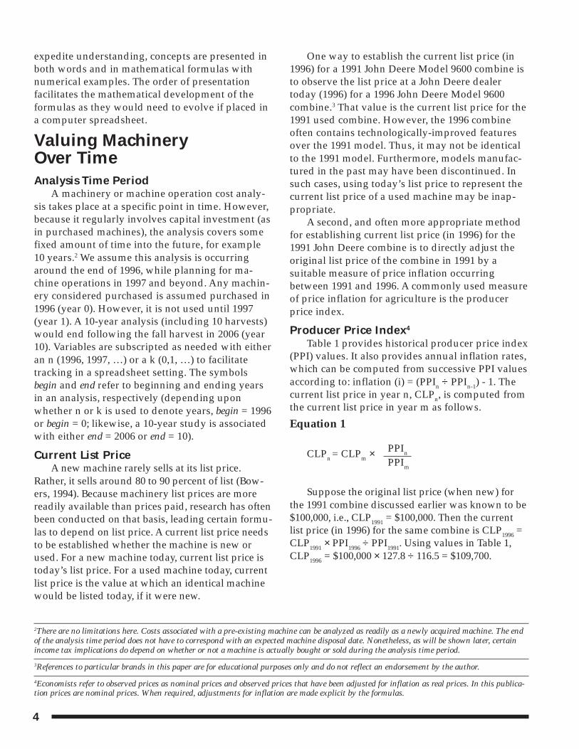
Because decisions based on machinery costanalysis are always forward-looking, expectationsfor future inflation rates are required. As an indica-tion of inflation level possibilities, Figure 1 depictsPPI-based inflation from 1950 through 1996 (1996value based on first 8 months). Most years, infla-

tion levels were in the 0 percent to 5 percent range,with a few years displaying negative inflation(deflation). Two inflation spikes during the 1970sstand out, along with the precipitous decline in theearly 1980s. Historically, the preceding year’sinflation has been a more reliable indicator of thecurrent year’s inflation than has been a longer-termmulti-year average. So, PPI values in Table 1 forfuture years assume the same inflation rate com-puted for 1996 (i = 0.02455, or around 2.5 percent).Thus, Equation 1 is also used to estimate currentlist price in future years. For example,CLP2006 = CLP1996 × PPI2006 ÷ PPI1996 = $109,700 ×162.9 ÷ 127.8 = $139,829. Because annual inflationrates are assumed to be the same over the 10 yearsfollowing 1996, the current list price in 1997 alsomay be determined with the formulaCLP2006 = CLP1996 × (1+ i)10 = $109,700 × (1.02455)10 =$109,700 × 1.2745 = $139,810, which is the same as$139,829 except for rounding errors.

Table 1. Producer Price Index, U.S. Average, All CommoditiesYear Index Inflation Year Index Inflation

1962 31.6500 0.00238 1985 103.1500 -0.005061963 31.5750 -0.00237 1986 100.1667 -0.028921964 31.6333 0.00185 1987 102.8083 0.026371965 32.2667 0.02002 1988 106.9417 0.040201966 33.3083 0.03228 1989 112.2417 0.049561967 33.4000 0.00275 1990 116.2917 0.036081968 34.2333 0.02495 1991 116.5333 0.002081969 35.5917 0.03968 1992 117.1917 0.005651970 36.9000 0.03676 1993 118.9083 0.014651971 38.1083 0.03275 1994 120.4500 0.012971972 39.7917 0.04417 1995 124.7583 0.035771973 45.0250 0.13152 1996 127.8205 0.024551974 53.4853 0.18786 1997 130.9579 0.024551975 58.4167 0.09224 1998 134.1723 0.024551976 61.1333 0.04650 1999 137.4656 0.024551977 64.8750 0.06121 2000 140.8397 0.024551978 69.9417 0.07810 2001 144.2966 0.024551979 78.7250 0.12558 2002 147.8384 0.024551980 89.8093 0.14079 2003 151.4671 0.024551981 98.0333 0.09158 2004 155.1849 0.024551982 100.0167 0.02023 2005 158.9939 0.024551983 101.2500 0.01233 2006 162.8964 0.024551984 103.6750 0.02395 2007 166.8947 0.02455

Source: Federal Reserve Bank of St. Louis FRED database (http://www.stls.frb.org/fred)Notes:1982=100, 1996 based on monthly indices through August, 1996.Years 1997-2007 assume same annual inflation rate estimated for 1996.

Figure 1

Annual Inflation Based on Producer Price Index, 1950–1996Figure 1.

Per

cent

(de

cim

al f

orm

)

0.2

0.15

0.1

0.05

0

-0.05

1950 1954 1958 1962 1966 1970 1974 1978 1982 1986 1990 1994

6

Remaining Value Percentage, EconomicDepreciation, and Market Value

Remaining value percentage (RVP) is thepercent (in decimal form) that a machine’s marketvalue is of its current list price (both evaluated inthe same year). RVP helps determine a machine’seconomic depreciation, which is the amount ofmarket value lost each year due to age, wear, andobsolescence (not to be confused with tax deprecia-tion). For a particular class of machinery, remainingvalue percentage is often assumed to be deter-mined by its age and not its rate of use, using aconstant rate of market value depreciation. Bowersuses the following formula developed by the Ameri-can Society of Agricultural Engineers (ASAE):

Equation 2RVPn = RVP1n = dep1 × dep2AGEn,

if AGEn ≥ 1, and 0.85 if AGEn < 1;

where RVPn is RVP in year n (the 1 following RVPdistinguishes the ASAE formula from an alterna-tive presented later), AGEn is a machine’s age inyears in year n. Depreciation factors for differentmachinery classes, dep1 and dep2, are in Table 2.Equation 2 states that with 0 inflation a machinedepreciates annually at the rate of (1-dep2). That is,each year it is worth dep2 as much as it was theyear before.

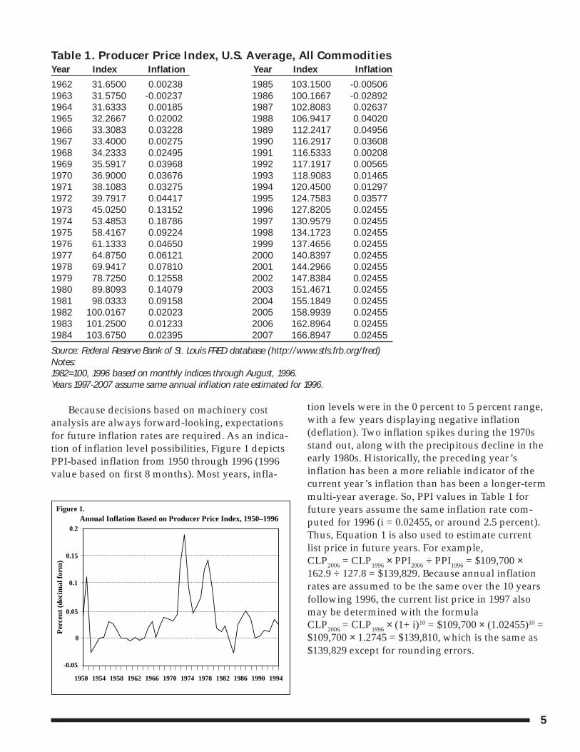
Figure 2 graphically shows RVP1 values com-puted from Equation 2 for several classes of ma-chinery. Planters and tillage equipment depreciatemore slowly than other classes, and at the end of 20years, are still worth 29 percent of their current listprices. On the other hand, balers are worth only 12percent of their current list prices at the end of 20years. Combines and tractors are in between.

Factors dep1 and dep2 in Equation 2 werecomputed with and are designed to be used withmachinery that is at least 1 year old. Thus, a condi-tional statement follows the formula in Equation 2.Without that conditional statement, because dep20

= 1, new machines would be estimated to cost dep1of current list price. The dep1 values in Table 2 aretoo low to appropriately value new machines.Instead, new machines are assumed to cost 85percent of their list prices.

Market value in year n, MVn, is the remainingvalue percentage times current list price:

Equation 3

MVn = CLPn × RVPn

Economic depreciation is the change in marketvalue across any 2 years, or MVn-MVn-1. Becausecurrent list price is affected by inflation, and be-cause remaining value percentage is a measure ofeconomic depreciation, Equation 3 shows that bothinflation and economic depreciation affect currentmarket value of machinery. If inflation is highenough to offset economic depreciation, causingCLP to rise rapidly over years, a used machine maysell for more than when it was new.

Continuing with the combine example, the 1996remaining value percentage is RVP11996 = dep1 ×dep2(1996-1991), or 0.65×0.935 = 0.4522. Inserting the$109,700 value for CLP1996 computed earlier, marketvalue in 1996 is MV1996 = $109,700 × 0.4522 = $49,606.

Equation 2 depicts economic depreciation as afixed cost relating to age. However, because wear isa function of rate of use, if rate of use varies acrossmachines and years, depreciation may have bothvariable and fixed cost components. For somemachines, most notably for combines, rate of usemay be as important for determining market valueas is age (Cross and Perry; Kastens, Featherstone,

Table 2. Factors for Calculating Remaining Value Percentages byMachinery Class.

Machinery ClassWindrowers Forage Planters/

Factor Tractors Combines Mowers Harvesters Balers Tillagedep1 0.67 0.65 0.67 0.56 0.66 0.66dep2 0.94 0.93 0.90 0.90 0.92 0.96Source: Machinery Replacement Strategies, by Wendell Bowers, Deere and Company, 1994, p.9Notes:Factors used to calculate remaining value from age: RVP=dep1 × dep2AGE.When age is 0 RVP is assumed to be 0.85.

7

and Biere). This is likely due to the number of usedcombines that have been originally owned bycustom harvesters. Such machines are typicallyused more intensely and traded more often thanfarmer-owned machines.

Recently, economists have begun to deriveformulas that attempt to quantify the relationshipbetween rate of use and market value, especiallyfor tractors and combines, where hour meters havebeen standard for many years. However, for tillageand planting equipment, historical rate of use isdifficult to quantify. For other classes, such asbalers, it may come about because of bale counters.Cross and Perry examined auction sale pricesreported monthly from January 1984 to June 1993in the Farm Equipment Guide (Hot Line, Inc.).Equipment manufactured between 1971 and 1993were considered. Their study resulted in the fol-lowing formula relating market value to age andrate of use:

Equation 4RVPn = RVP2n = (a+b × (AGEn)

c + d × (HPYn)e)f,

if AGEn ≥ 1, and 0.85 if AGEn < 1.

Equation 4 depicts an alternative method toEquation 2 for computing remaining value percent-age that considers rate of use as well as age. LikeRVP1n in Equation 2, RVP2n is the proportion(ranging between 0 and 1) that the projected mar-ket value in year n is of the current list price in yearn. AGEn is machine age in years at year n. HPYn isthe average hours per year that the machine wasused since it was new, evaluated in year n, or AHn

÷ AGEn , where AHn denotes the accumulatedhours on the machine as of year n. The smallletters, a, b, c, d, e, and f are factors required of theformula. Factor values for several brands of trac-tors, combines, disks, planters, swathers, andbalers are in Table 3.5 Like Equation 2, Equation 4requires the conditional statement to value equip-ment properly when it is less than 1 year old.

Assume the 1991 John Deere combine had 4,000hours on its hour meter in 1996 so that HPY1996 =4000 ÷ 5 = 800.6 Using the appropriate values fromTable 3, Equation 4 predicts a remaining valuepercentage of RVP21996 = [0.94692 - 0.04551 × 50.87 –0.00182 × 8000.72]2 = 0.2899. Using the 1996 currentlist price computed earlier of $109,700, along withEquations 3 and 4, the 1991 machine with 4,000hours is expected to have a 1996 market value of$31,802. This is substantially less than the $49,606value computed from Equation 2, partly because ofthe machine’s high usage rate. On the other hand, ifthe usage rate were 200 hours per year (more typicalof a farmer owned machine) rather than 800, Equa-tion 4 predicts a remaining value percentage of0.4621, yielding a market value of $50,692, muchcloser to the value calculated using Equation 2.

5For tractors, in order to allow for horsepower to affect remaining value, the factor a reported in Table 3 must be modified slightly beforeusing in Equation 4. Specifically, for 80-149 horsepower tractors, the value, 0.00046 × pto horsepower, must be subtracted from the associ-ated a values before they can be used in Equation 4. For 150+ horsepower tractors, the value, 0.00093 × pto horsepower, must be subtractedfrom the associated a values. For all other machinery classes in Table 3, the a’s are used as they appear. Formulas reported by Cross and Perryincluded several additional measures besides age and usage to determine remaining value. Equation 4 was deduced by holding these othermeasures constant. Thus, it depicts the remaining value percentage for equipment in good condition (contrasted with excellent, fair, or poor)sold at retirement auctions (contrasted with consignment, bankruptcy, or dealer closeout) in the Middle Great Plains (South Dakota,Nebraska, and Kansas).

6Machinery purchases are assumed to occur at the end of the year. That is, the 4,000 hours are assumed to have accumulated over harvestyears, 1992, 1993, 1994, 1995, and 1996. Recent-model combines measure both engine hours and separator hours. Because research-basedformulas are based on engine hours that is what is assumed here.

Remaining Value as a Percent of Current List Price by Age, for Several Machinery Classes

Figure 2.P

erce

nt (

deci

mal

for

m)

0.7

0.6

0.5

0.4

0.3

0.2

0.1

0

1

Age in Years2 3 4 5 6 7 8 9 10 11 12 13 14 15 16 17 18 19 20

Tractor Combine

Planter, Tillage Baler

8

Table 3. Cross and Perry Adjustment Factorsfor Selected Machinery Classes and Manufacturers

Adjustment Factorsa* b c d e f

80-149 HP TractorsAC 0.969772 -0.02725 0.76 -0.00236 0.6 3.846154Case 1.000787 -0.03277 0.76 -0.00120 0.6 3.846154Ford 1.029438 -0.02768 0.76 -0.00275 0.6 3.846154Deere 1.035260 -0.02301 0.76 -0.00120 0.6 3.846154IH 0.989220 -0.02765 0.76 -0.00203 0.6 3.846154MF 0.997552 -0.02909 0.76 -0.00261 0.6 3.846154White 1.032797 -0.02891 0.76 -0.00371 0.6 3.846154

150+ HP TractorsAC 1.305504 -0.22785 0.35 -0.01187 0.39 2.222222Case 1.462469 -0.30023 0.35 -0.01020 0.39 2.222222Ford 1.238971 -0.11517 0.35 -0.01500 0.39 2.222222Deere 1.405956 -0.22231 0.35 -0.00766 0.39 2.222222IH 1.340365 -0.26484 0.35 -0.00547 0.39 2.222222MF 1.282532 -0.26106 0.35 -0.00155 0.39 2.222222White 1.408643 -0.25439 0.35 -0.01413 0.39 2.222222

CombinesAC 0.843972 -0.03779 0.87 -0.00244 0.72 2.0Case 0.893689 -0.04679 0.87 -0.00091 0.72 2.0Ford 1.746431 -0.12208 0.87 -0.00771 0.72 2.0Deere 0.946917 -0.04551 0.87 -0.00182 0.72 2.0IH 0.925632 -0.04411 0.87 -0.00243 0.72 2.0MF 0.753825 -0.03811 0.87 -0.00117 0.72 2.0White 0.792664 -0.03479 0.87 -0.00373 0.72 2.0NH 0.905448 -0.06141 0.87 -0.00105 0.72 2.0

DisksDeere 0.364825 0.60697 -0.85 0 0 2.040816IH 0.445666 0.55410 -0.85 0 0 2.040816MF 0.216219 1.95014 -0.85 0 0 2.040816Kewanee 0.031970 3.06544 -0.85 0 0 2.040816Krause 0.215375 1.39979 -0.85 0 0 2.040816

PlantersDeere 0.867382 -0.01939 0.89 0 0 1.960784IH 0.924203 -0.04245 0.89 0 0 1.960784

SwathersDeere 0.855234 -0.04564 0.50 0 0 5.263158IH 1.077101 -0.10692 0.50 0 0 5.263158NH 1.062699 -0.10301 0.50 0 0 5.263158Hesston 0.959780 -0.06955 0.50 0 0 5.263158

BalersDeere 0.814355 -0.05939 0.57 0 0 2.777778IH 1.152865 -0.08524 0.57 0 0 2.777778NH 0.774934 -0.06093 0.57 0 0 2.777778Hesston 0.895971 -0.10806 0.57 0 0 2.777778

Source: Cross, T.L. and G.M. Perry. “Depreciation Patterns for Agricultural Machinery.” American Journal of AgriculturalEconomics. 77(February, 1995):194-204.*For 80 to 149 horsepower tractors, the value 0.00046 × hp must be subtracted from the a factor shown in the table, where hpis the pto horsepower for the tractor considered. For 150+ horsepower tractors, subtract 0.00093 × hp. For other classes ofmachinery use the a values as they appear.

9

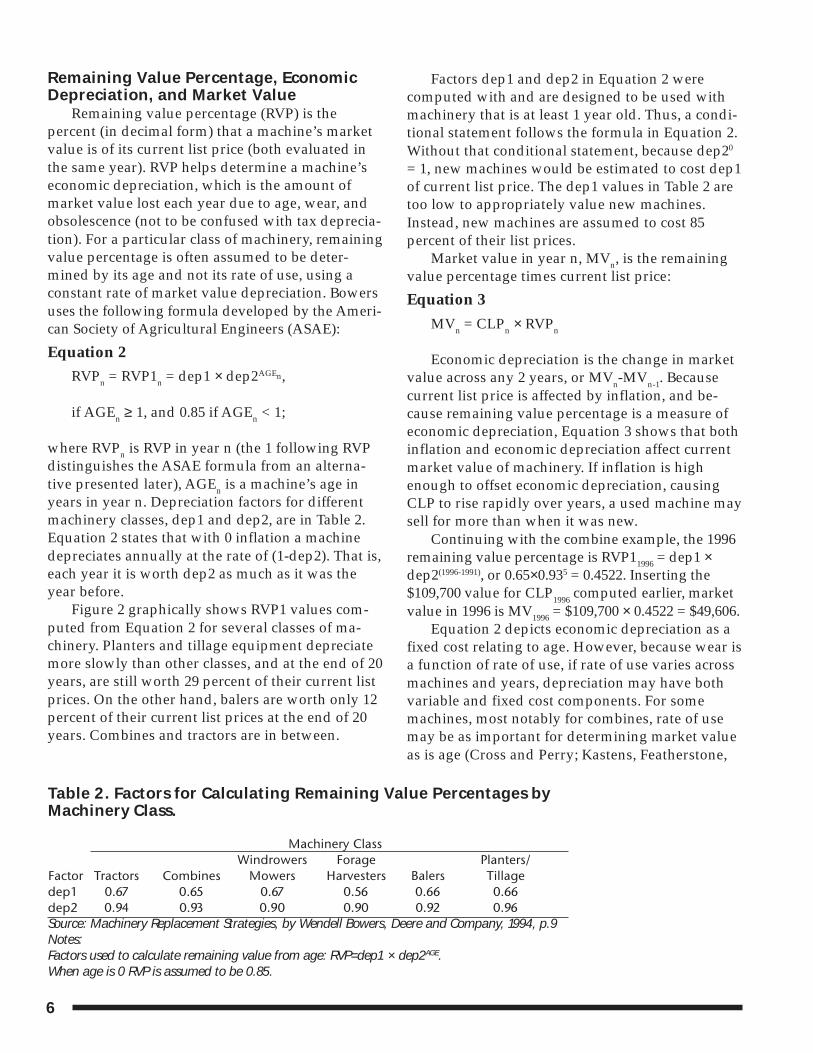
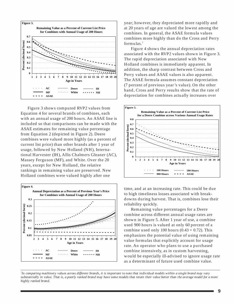
Figure 3 shows computed RVP2 values fromEquation 4 for several brands of combines, eachwith an annual usage of 200 hours. An ASAE line isincluded so that comparisons can be made with theASAE estimates for remaining value percentagefrom Equation 2 (depicted in Figure 2). Deerecombines were valued more highly (as a percent ofcurrent list price) than other brands after 1 year ofusage, followed by New Holland (NH), Interna-tional Harvester (IH), Allis Chalmers Gleaner (AC),Massey Ferguson (MF), and White. Over the 20years, except for New Holland, the relativerankings in remaining value are preserved. NewHolland combines were valued highly after one

year; however, they depreciated more rapidly andat 20 years of age are valued the lowest among thecombines. In general, the ASAE formula valuescombines more highly than do the Cross and Perryformulas.7

Figure 4 shows the annual depreciation ratesassociated with the RVP2 values shown in Figure 3.The rapid depreciation associated with NewHolland combines is immediately apparent. Inaddition, the sharp contrast between Cross andPerry values and ASAE values is also apparent.The ASAE formula assumes constant depreciation(7 percent of previous year’s value). On the otherhand, Cross and Perry results show that the rate ofdepreciation for combines actually increases over

time, and at an increasing rate. This could be dueto high timeliness losses associated with break-downs during harvest. That is, combines lose theirreliability quickly.

Remaining value percentages for a Deerecombine across different annual usage rates areshown in Figure 5. After 1 year of use, a combineused 900 hours is valued at only 60 percent of acombine used only 100 hours (0.43 ÷ 0.72). Thisemphasizes the potential value of using remainingvalue formulas that explicitly account for usagerate. An operator who plans to use a purchasedcombine intensively, as in custom harvesting,would be especially ill-advised to ignore usage rateas a determinant of future used combine value.

7In comparing machinery values across different brands, it is important to note that individual models within a single brand may varysubstantially in value. That is, a poorly ranked brand may have some models that retain their value better than the average model for a morehighly ranked brand.

Remaining Value as a Percent of Current List Price for Combines with Annual Usage of 200 Hours

Figure 3.P

erce

nt (

deci

mal

for

m)

0.7

0.6

0.5

0.4

0.3

0.2

0.1

01

Age in Years2 3 4 5 6 7

ASAEMF

AC Deere IHNHWhite

8 9 10 11 12 13 14 15 16 17 18 19 20

Annual Depreciation as a Percent of Previous Year's Pricefor Combines with Annual Usage of 200 Hours

Figure 4.

Per

cent

(de

cim

al f

orm

)

0.3

0.25

0.2

0.15

0.1

0.05

Age in Years2 3 4 5 6 7

ASAEMF

AC Deere IHNHWhite

8 9 10 11 12 13 14 15 16 17 18 19 20

Remaining Value as a Percent of Current List Pricefor a Deere Combine across Various Annual Usage Rates

Figure 5.

Perc

ent (

deci

mal

form

)

0.8

0.7

0.6

Age in Years

900 Hours

100 Hours 500 HoursASAE

0.5

0.4

0.3

0.2

0.1

02 3 4 5 6 7 8 9 10 11 12 13 14 15 16 17 18 19 201

10

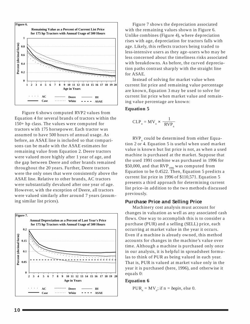
Figure 6 shows computed RVP2 values fromEquation 4 for several brands of tractors within the150+ hp class. The values were computed fortractors with 175 horsepower. Each tractor wasassumed to have 500 hours of annual usage. Asbefore, an ASAE line is included so that compari-sons can be made with the ASAE estimates forremaining value from Equation 2. Deere tractorswere valued more highly after 1 year of age, andthe gap between Deere and other brands remainedthroughout the 20 years. Further, Deere tractorswere the only ones that were consistently above theASAE line. Relative to other brands, AC tractorswere substantially devalued after one year of age.However, with the exception of Deere, all tractorswere valued similarly after around 7 years (assum-ing similar list prices).

Figure 7 shows the depreciation associatedwith the remaining values shown in Figure 6.Unlike combines (Figure 4), where depreciationrises with age, depreciation for tractors falls withage. Likely, this reflects tractors being traded toless-intensive users as they age–users who may beless concerned about the timeliness risks associatedwith breakdowns. As before, the curved deprecia-tion paths contrast sharply with the straight linefor ASAE.

Instead of solving for market value whencurrent list price and remaining value percentageare known, Equation 3 may be used to solve forcurrent list price when market value and remain-ing value percentage are known:

Equation 5

CLPn = MVn ×1

RVPn

RVPn could be determined from either Equa-tion 2 or 4. Equation 5 is useful when used marketvalue is known but list price is not, as when a usedmachine is purchased at the market. Suppose thatthe used 1991 combine was purchased in 1996 for$50,000, and that RVP1996 was computed fromEquation to be 0.4522. Then, Equation 5 predicts acurrent list price in 1996 of $110,571. Equation 5presents a third approach for determining currentlist price–in addition to the two methods discussedpreviously.

Purchase Price and Selling PriceMachinery cost analysis must account for

changes in valuation as well as any associated cashflows. One way to accomplish this is to consider apurchase (PUR) and a selling (SELL) price, eachoccurring at market value in the year it occurs.Even if a machine is already owned, this methodaccounts for changes in the machine’s value overtime. Although a machine is purchased only oncein our analysis, it is helpful in spreadsheet formu-las to think of PUR as being valued in each year.That is, PUR is valued at market value only in theyear it is purchased (here, 1996), and otherwise itequals 0:

Equation 6

PURn = MVn; if n = begin, else 0.

Remaining Value as a Percent of Current List Pricefor 175 hp Tractors with Annual Usage of 500 Hours

Figure 6.

Per

cent

(de

cim

al f

orm

)

1

0

Age in Years2 3 4 5 6 7

Case

AC Deere IHWhite

8 9 10 11 12 13 14 15 16 17 18 19 20

0.8

0.6

0.4

0.2

1

ASAE

Annual Depreciation as a Percent of Last Year's Pricefor 175 hp Tractors with Annual Usage of 500 Hours

Figure 7.

Per

cent

(de

cim

al f

orm

)

Age in Years2 3 4 5 6 7

Case

AC Deere IH

White

8 9 10 11 12 13 14 15 16 17 18 19 20

0.2

0.15

0.1

0.05

0

ASAE

11

Similarly, the selling price in year n, SELLn , is

Equation 7SELLn = MVn; if n = end, else 0.

Annual Operating CostsField Efficiency

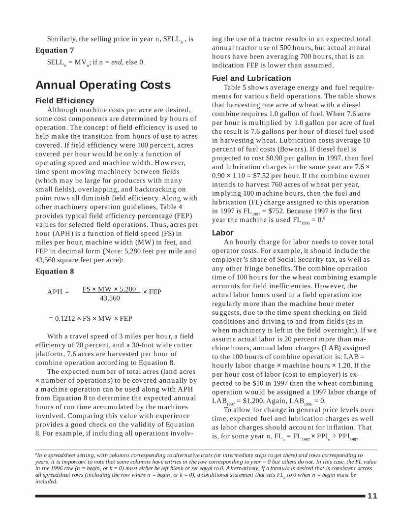
Although machine costs per acre are desired,some cost components are determined by hours ofoperation. The concept of field efficiency is used tohelp make the transition from hours of use to acrescovered. If field efficiency were 100 percent, acrescovered per hour would be only a function ofoperating speed and machine width. However,time spent moving machinery between fields(which may be large for producers with manysmall fields), overlapping, and backtracking onpoint rows all diminish field efficiency. Along withother machinery operation guidelines, Table 4provides typical field efficiency percentage (FEP)values for selected field operations. Thus, acres perhour (APH) is a function of field speed (FS) inmiles per hour, machine width (MW) in feet, andFEP in decimal form (Note: 5,280 feet per mile and43,560 square feet per acre):

Equation 8

APH = FS × MW × 5,280 × FEP43,560

= 0.1212 × FS × MW × FEP

With a travel speed of 3 miles per hour, a fieldefficiency of 70 percent, and a 30-foot wide cutterplatform, 7.6 acres are harvested per hour ofcombine operation according to Equation 8.

The expected number of total acres (land acres× number of operations) to be covered annually bya machine operation can be used along with APHfrom Equation 8 to determine the expected annualhours of run time accumulated by the machinesinvolved. Comparing this value with experienceprovides a good check on the validity of Equation8. For example, if including all operations involv-

ing the use of a tractor results in an expected totalannual tractor use of 500 hours, but actual annualhours have been averaging 700 hours, that is anindication FEP is lower than assumed.

Fuel and LubricationTable 5 shows average energy and fuel require-

ments for various field operations. The table showsthat harvesting one acre of wheat with a dieselcombine requires 1.0 gallon of fuel. When 7.6 acreper hour is multiplied by 1.0 gallon per acre of fuelthe result is 7.6 gallons per hour of diesel fuel usedin harvesting wheat. Lubrication costs average 10percent of fuel costs (Bowers). If diesel fuel isprojected to cost $0.90 per gallon in 1997, then fueland lubrication charges in the same year are 7.6 ×0.90 × 1.10 = $7.52 per hour. If the combine ownerintends to harvest 760 acres of wheat per year,implying 100 machine hours, then the fuel andlubrication (FL) charge assigned to this operationin 1997 is FL1997 = $752. Because 1997 is the firstyear the machine is used FL1996 = 0.8

LaborAn hourly charge for labor needs to cover total

operator costs. For example, it should include theemployer’s share of Social Security tax, as well asany other fringe benefits. The combine operationtime of 100 hours for the wheat combining exampleaccounts for field inefficiencies. However, theactual labor hours used in a field operation areregularly more than the machine hour metersuggests, due to the time spent checking on fieldconditions and driving to and from fields (as inwhen machinery is left in the field overnight). If weassume actual labor is 20 percent more than ma-chine hours, annual labor charges (LAB) assignedto the 100 hours of combine operation is: LAB =hourly labor charge × machine hours × 1.20. If theper hour cost of labor (cost to employer) is ex-pected to be $10 in 1997 then the wheat combiningoperation would be assigned a 1997 labor charge ofLAB1997 = $1,200. Again, LAB1996 = 0.

To allow for change in general price levels overtime, expected fuel and lubrication charges as wellas labor charges should account for inflation. Thatis, for some year n, FLn = FL1997 × PPIn ÷ PPI1997.

8In a spreadsheet setting, with columns corresponding to alternative costs (or intermediate steps to get there) and rows corresponding toyears, it is important to note that some columns have entries in the row corresponding to year = 0 but others do not. In this case, the FL valuein the 1996 row (n = begin, or k = 0) must either be left blank or set equal to 0. Alternatively, if a formula is desired that is consistent acrossall spreadsheet rows (including the row where n = begin, or k = 0), a conditional statement that sets FL

n to 0 when n = begin must be

included.

12

Table 4. Field Efficiency, Field Speed, and Repair and Maintenance Factorsfor Field Operations

Field Efficiency Field Speed EUL Repair FactorsRange Typical Range Typical Est. Life Tot. Life

% % mph mph hours Cost%a RF1 RF2TRACTORS2WD & stationary 12,000 100 0.007 2.04WD & crawler 16,000 80 0.003 2.0

TILLAGE & PLANTMoldboard plow 70-90 85 3.0-6.0 4.5 2,000 100 0.29 1.8Heavy-duty disk 70-90 85 3.0-6.0 4.5 2,000 60 0.18 1.7Tandem disk harrow 70-90 80 4.0-7.0 6.0 2,000 60 0.18 1.7(Coulter) chisel plow 70-90 85 4.0-6.5 5.0 2,000 75 0.28 1.4Field Cultivator 70-90 85 5.0-8.0 7.0 2,000 70 0.27 1.4Spring tooth harrow 70-90 85 5.0-8.0 7.0 2,000 70 0.27 1.4Roller-packer 70-90 85 4.5-7.5 6.0 2,000 40 0.16 1.3Mulcher-packer 70-90 80 4.0-7.0 5.0 2,000 40 0.16 1.3Rotary hoe 70-85 80 8.0-14.0 12.0 2,000 60 0.23 1.4Row crop cultivator 70-90 80 3.0-7.0 5.0 2,000 80 0.17 2.2Rotary tiller 70-90 85 1.0-4.5 3.0 1,500 80 0.36 2.0Row crop planter 50-75 65 4.0-7.0 5.5 1,500 75 0.32 2.1Grain drill 55-80 70 4.0-7.0 5.0 1,500 75 0.32 2.1

HARVESTINGCorn picker sheller 60-75 65 2.0-4.0 2.5 2,000 70 0.14 2.3PT Combine 60-75 65 2.0-5.0 3.0 2,000 60 0.12 2.3SP Combine 65-80 70 2.0-5.0 3.0 3,000 40 0.04 2.1Mower 75-85 80 3.0-6.0 5.0 2,000 150 0.46 1.7Mower (rotary) 75-90 80 5.0-12.0 7.0 2,000 175 0.44 2.0Mower-conditioner 75-85 80 3.0-6.0 5.0 2,500 80 0.18 1.6Mow-cond (rotary) 75-90 80 5.0-12.0 7.0 2,500 100 0.16 2.0SP Windrower 70-85 80 3.0-8.0 5.0 3,000 55 0.06 2.0Side delivery rake 70-90 80 4.0-8.0 6.0 2,500 60 0.17 1.4Square baler 60-85 75 2.5-6.0 4.0 2,000 80 0.23 1.8Large square baler 70-90 80 4.0-8.0 5.0 3,000 75 0.10 1.8Large round baler 55-75 65 3.0-8.0 5.0 1,500 90 0.43 1.8Forage harvester 60-85 70 1.5-5.0 3.0 2,500 65 0.15 1.6SP Forage harvester 60-85 70 1.5-6.0 3.5 4,000 50 0.03 2.0Sugar beet harvester 50-70 60 4.0-6.0 5.0 1,500 100 0.59 1.3Potato harvester 55-70 60 1.5-4.0 2.5 2,500 70 0.19 1.4SP Cotton picker 60-75 70 2.0-4.0 3.0 3,000 80 0.11 1.8

MISCELLANEOUSFertilizer spreader 60-80 70 5.0-10.0 7.0 1,200 80 0.63 1.3Boom-type sprayer 50-80 65 3.0-7.0 6.5 1,500 70 0.41 1.3Bean puller/windrower 70-90 80 4.0-7.0 5.0 2,000 60 0.20 1.6Beet topper/chopper 70-90 80 4.0-7.0 5.0 1,200 35 0.28 1.4

Source: ASAE Standards 1993, American Society of Agricultural Engineers, St. Joseph, Michigan, 1993, p.332.a percent of current list price

13

Similarly, LABn = LAB1997 × PPIn ÷ PPI1997. Forexample, in 2003, fuel and lubrication charges areexpected to be FL2003 = $752 × 151.5 ÷ 131.0 = $870,where PPI values are taken from Table 1.

Repair and MaintenanceThe ASAE describes accumulated charges for

repair and maintenance (ARM) for a particularmachine as a function of the machine’s current listprice, accumulated use of the machine in hours(AH), and two factors specific to the machine, RF1and RF2. However, if a machine’s hours are be-yond its estimated useful life (EUL)–a convenientmathematical threshold, not necessarily indicativeof limits to use–then the machine is assumed toaccumulate repairs at the same hourly rate it didwhen at its estimated useful life. Values for RF1,RF2, and EUL are found in Table 4. The formulathat calculates a machine’s accumulated repair andmaintenance costs is

Equation 9

ARMn =RF1 × CLPn × (AHn)RF2

, if AHn ≤ EUL1,000

else,

RF1 × CLPn × (EUL)RF2 ×1,000

[1 + RF2 × (AHn–EUL) ] , if AHn > EULEUL

Suppose that the hour meter on the 1991 JohnDeere combine displayed 1,000 hours when it waspurchased in 1996 . Assuming that the future usagerate will be 200 hours per year, then AH1997 = 1,200and AH2003 = 2,400. The repair and maintenancecharge for a particular year n, RMn, is defined as:9

Equation 10

RMn = ARMn – ARMn–1; if n > begin, else 0

We know that CLP1996 = $109,700, and fromEquation 1, CLP1997 = CLP1996 × PPI1997 ÷ PPI1996 =$109,700 × 131.0 ÷ 127.8 = $112,447. Table 4 showsthat, for a self-propelled combine, RF1 and RF2 are0.04 and 2.1, respectively. Then, using Equation 9and Equation 10, the repair charge for 1997 is:

RM1997 = [0.04 × $112,447 × (1200 ÷ 1000)2.1] – [0.04 ×$109,700 × (1000 ÷ 1000)2.1] = $6,596 – $4,388 =$2,208.

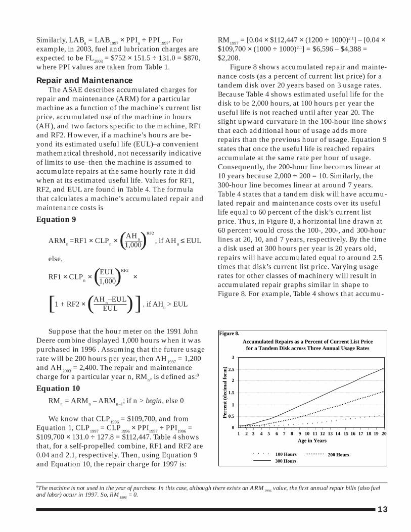
Figure 8 shows accumulated repair and mainte-nance costs (as a percent of current list price) for atandem disk over 20 years based on 3 usage rates.Because Table 4 shows estimated useful life for thedisk to be 2,000 hours, at 100 hours per year theuseful life is not reached until after year 20. Theslight upward curvature in the 100-hour line showsthat each additional hour of usage adds morerepairs than the previous hour of usage. Equation 9states that once the useful life is reached repairsaccumulate at the same rate per hour of usage.Consequently, the 200-hour line becomes linear at10 years because 2,000 ÷ 200 = 10. Similarly, the300-hour line becomes linear at around 7 years.Table 4 states that a tandem disk will have accumu-lated repair and maintenance costs over its usefullife equal to 60 percent of the disk’s current listprice. Thus, in Figure 8, a horizontal line drawn at60 percent would cross the 100-, 200-, and 300-hourlines at 20, 10, and 7 years, respectively. By the timea disk used at 300 hours per year is 20 years old,repairs will have accumulated equal to around 2.5times that disk’s current list price. Varying usagerates for other classes of machinery will result inaccumulated repair graphs similar in shape toFigure 8. For example, Table 4 shows that accumu-

9The machine is not used in the year of purchase. In this case, although there exists an ARM1996 value, the first annual repair bills (also fueland labor) occur in 1997. So, RM

1996 = 0.

Accumulated Repairs as a Percent of Current List Pricefor a Tandem Disk across Three Annual Usage Rates

Figure 8.

Per

cent

(de

cim

al f

orm

)

Age in Years3 4 5 6 7

100 Hours 200 Hours300 Hours

8 9 20

3

2

1

0

2.5

1.5

0.5

21 10 11 12 13 14 15 16 17 18 19

14

Table 5. Average Energy and Fuel Requirements for Selected Machinery OperationsGasoline Diesel LP Gas

Avg fuel consump. per max pto hp (gal per hr)> 0.068 0.044 0.08Field Operation PTO hp-hrs/acre Gasoline gal/acre Diesel gal/acre LP Gas gal/acreShred stalks 10.5 1.00 0.72 1.20Plow 8-in deep 24.4 2.35 1.68 2.82Heavy offset disk 13.8 1.33 0.95 1.60Chisel Plow 16.0 1.54 1.10 1.85Tandem disk, stalks 6.0 0.63 0.45 0.76Tandem disk, chiseled 7.2 0.77 0.55 0.92Tandem disk, plowed 9.4 0.91 0.65 1.09Field cultivate 8.0 0.84 0.60 1.01Spring-tooth harrow 5.2 0.56 0.40 0.67Spike-tooth harrow 3.4 0.42 0.30 0.50Rod weeder 4.0 0.42 0.30 0.50Sweep plow 8.7 0.84 0.60 1.01Cultivate row crops 6.0 0.63 0.45 0.76Rolling Cultivator 3.9 0.49 0.35 0.59Rotary hoe 2.8 0.35 0.25 0.42Anhydrous applicator 9.4 0.91 0.65 1.09Planting row crops 6.7 0.70 0.50 0.84No-till planter 3.9 0.49 0.35 0.59Till plant (with sweep) 4.5 0.56 0.40 0.67Grain drill 4.7 0.49 0.35 0.59Combine (small grains) 11.0 1.40 1.00 1.68Combine, beans 12.0 1.54 1.10 1.85Combine, corn & milo 17.6 2.24 1.60 2.69Corn picker 12.6 1.61 1.15 1.93Mower (cutterbar) 3.5 0.49 0.35 0.59Mower conditioner 7.2 0.84 0.60 1.01Swather 6.6 0.77 0.55 0.92Rake, single 2.5 0.35 0.25 0.42Rake, tandem 1.5 0.21 0.15 0.25Baler 5.0 0.63 0.45 0.76Stack wagon 6.0 0.70 0.50 0.84Sprayer 1.0 0.14 0.10 0.17Rotary Mower 9.6 1.12 0.80 1.34Haul small grains 6.0 0.84 0.60 1.01Grain drying 84.0 8.40 6.00 10.08Forage harvester, green 12.4 1.33 0.95 1.60Forage harv, haylage 16.3 1.75 1.25 2.10Forage harvester, corn 46.7 5.04 3.60 6.05Forage blower, haylage 3.3 0.35 0.25 0.42Forage blower, corn silage 18.2 1.96 1.40 2.35

Source: Machinery Replacement Strategies, by Wendell Bowers, Deere and Company, 1994, p.80,81.

15

lated self-propelled combine repairs will reach 40percent of current list price when the combine hasaccumulated 3,000 hours.

In practice, repair and maintenance costs varysubstantially across operators due to differences inmanagement styles. One producer may spend littletime on maintenance, hoping that gains in timeli-ness offset potential additional repairs. Others maybe especially careful with maintenance, believingthat the extra labor costs will be offset by reducedrepair costs. Thus, a personal repair adjustmentfactor (RAF), may be multiplied by the RMn inEquation 10 to better represent true repair cost.Bowers suggests that actual repair and mainte-nance costs may vary as much as ± 25 percent fromthose computed by Equation 10. Consequently,RAF is valued at something between 0.75 and 1.25,and Equation 10 is modified to:

Equation 11RMn = (ARMn – ARMn-1) × RAF; if n > begin, else 0

The repair and maintenance value establishedin Equation 11 does not require adjustment forinflation because the embedded CLP value alreadyaccounts for it. It should be noted that the RAFshould not be made excessively low just becauseprojected current repairs in a spreadsheet settingappear high ten years from now. This is becauseinflation is easy to understand after it has beenexperienced, but often is more difficult to believeinto the future. Even a relatively modest inflationrate of 3 percent (low by historical standards as theaverage PPI-based inflation from 1963 through1995 was 4.3 percent) translates a current (1996)repair bill of $1,000 into $1,344 10 years from now–without any consideration for the additionalrepairs required of an aging machine.

Repair and maintenance values derived fromEquation 11 may also appear “too high” if they arecompared to traditional repair and maintenancecategories in farm accounting systems. Such ac-counts may not include the labor portion of repairsand maintenance provided on farm. Also, theymay not account for items such as depreciation onfarm shop tools and farm shop buildings. Conse-quently, absent a detailed understanding of histori-cal on-farm repair costs, it is appropriate to use thevalues from Equation 11 with RAF set to 1.0.

Equations 9 through 11 do not account forrepairs covered by warranties. Thus, for age orusage rates within warranty periods a furtheradjustment of Equation 11 is required to subtractout any warranty coverage of repairs and mainte-nance. Because the adjustment is highly machine-specific it is not included.

TimelinessTimeliness costs are associated with a reduction

in quantity or quality of crops harvested resultingfrom operations not being performed at optimaltimes. For some operations, such as planting orharvesting, timeliness costs may rise rapidly afteroptimal time periods are exceeded. Because timeli-ness costs are highly location-, crop-, and year-specific (timeliness costs may be especially high inwet years) they are not generalized in formulashere. However, careful comparisons betweenexperience and calculated annual machine hoursshould provide clues to potential timeliness prob-lems. For example, if it is known that a wheatharvest lasting longer than 10 days normallyresults in excessive yield losses, and a wheatcombine cost analysis projects annual machinehours of 200, then purchasing a larger combineshould be considered. More specifically, comparingthe per acre costs for a small combine requiring 12days to complete harvest with those of a largercombine (with higher per acre costs), requiringonly 10 days, results in a break-even crop loss thatcould be tolerated with the lower capacity ma-chine. The break-even crop loss can be comparedwith the expected loss associated with harvesting2 days longer than the optimal harvest period tohelp select the most profitable combine.

Using Equation 4 for remaining value calcula-tions, which explicitly accounts for usage rate, maylessen some of the problems associated with inad-equately accounting for timeliness costs. Specifi-cally, although per acre depreciation costs rise withless intensive use (since depreciation is spread overfewer acres), Equation 2 depicts a greater rise inper acre depreciation costs with less intensive usethan does Equation 4. In short, Equation 4 assignsless penalty for operating machinery that appearsoversized due to omitting timeliness costs, whichmeans an operator may choose slightly largermachinery by using Equation 4, which helps coverrisks associated with timeliness.

16

Property Taxes, Insurance, and ShelterTaxes (property taxes, not income taxes) insur-

ance, and shelter (TIS) are typically considered afixed machinery cost (usually a set percentage ofmarket value). However, if market value dependson usage rate, as in Equation 4, then even TIS hasvariable cost components. Presently (1996) Kansashas no property tax on farm machinery, so onlyinsurance and shelter must be considered. Weassume TIS is 1.5 percent of market value. Becausemarket value already accounts for inflation, noadditional adjustment is required. The TISn for-mula (with n beginning in 1997, so TIS1996 = 0) is

Equation 12TISn = MVn × 0.015

Income Tax and FinanceMarginal Tax Rates

In general, a marginal tax rate is the amount ofincome-related taxes that must be paid on the lastdollar of taxable profit. Because machinery deci-sions affect several years in the future, an expectedmarginal rate should be used, rather than thespecific rate applied to a single year. Furthermore,because some machinery costs offset self-employ-ment income and others offset only capital gains ordepreciation recapture, it is useful to consider twomarginal tax rates. The first rate, T1, includes bothfederal and state income tax rates. The second rate,T2, includes the self-employment tax as well.

Suppose a sole proprietor oscillates between amarginal federal rate of 0.15 one half of the timeand 0.28 the other half of the time. Then, the ex-pected marginal federal rate is 0.215. Combining0.215 with a Kansas income tax rate of around0.0485 implies T1 = 0.2635. Self-employment taxesare presently 0.1513. However, because one half ofself employment taxes are income tax deductible,the net self-employment tax rate is SE = 0.1513 –1/2 (0.1513) × T1 = 0.1365. Because T2 is the sum offederal and state income tax rates, plus the self-employment tax rate, T2 = T1 + SE = 0.2635 +0.1365 = 0.40. This rate effectively makes after-taxcost for expenses such as fuel and repairs only 60

percent of the cash outlays associated with thoseexpenses. Because farm corporations do not payself employment taxes, for them T2 = T1.10

Cost of CapitalMachinery is purchased with debt funds,

equity funds, or some combination of the two.When debt funds are used there is an explicitinterest charge. The cost of debt funds is the rate atwhich machinery investment funds may be bor-rowed. When equity funds are used there is animplicit charge referred to as opportunity cost.That is, equity funds could have been used else-where in the operation (as in expansion), or inoutside investment (such as in the stock market).The opportunity cost of equity funds is oftenconsidered to be the average or expected rate ofreturn on equity. Because interest is tax deductible,and because producers are ultimately interested inafter-tax income, the cost of capital rate is oftenreduced by the marginal tax rate, making it anafter-tax cost of capital rate.

One way to reduce the cost of capital (COC) toa single value is to weight the cost of debt by thelong run portion of debt used in the operation, andthe cost of equity by the long run portion of equityin the operation. Let Ke be the typical annual rateof return on equity for the farm, that is, the averageannual net farm income (before paying incometaxes, but after accounting for any charges forunpaid labor, and after accounting for economicdepreciation or appreciation of capital items),divided by the net worth at the beginning of theyear. Let Kd be the annual interest rate charged by alender on machinery loans. Let Wd be the percent-age of debt funds typically used in the operation(average debt to assets ratio). Then, cost of capitalcan be described by

Equation 13COC = [Ke × (1–Wd) + Kd × Wd] × (1 – T2)

The 1- T2 term at the right of Equation 13shows that the calculated COC is an after-tax rate.If a farm has a typical debt to assets ratio of 0.6 anda typical return on equity of 0.12, and the lender’sinterest rate is 0.10, then using the tax rate of T2 =0.40 implies that COC = [0.12 × (1 - 0.60) + 0.10 ×0.40] × (1 - 0.40) = 0.0648.

10This is most relevant for corporations that tend to use profits to build farm equity rather than pay out profits to their shareholders in theform of wages or dividends.

17

In general, it should be the case that Ke ≥ Kd

because it is highly unlikely that the long-runreturn on farm equity would be lower than thelong-run interest rate on loans. If it were, equityfunds would be used to pay down debt. Likewise,it is also unlikely that the long-run return on equitywould be substantially higher than the long-runinterest rate on loans. If it were, producers woulddemand more loans, causing the interest rate torise. In short, market forces tend to keep the inter-est rate on loans near the rate of return on farmequity. Equation 13 can be simplified by definingthe cost of capital as only the after-tax interest rateon machinery loans, or COC = Kd × (1 - T2).

Closely related to cost of capital is real cost ofcapital (or, real interest rate). Where i denotesinflation, the real cost of capital is defined as [(1 +COC) ÷ (1+i)] - 1, and represents the cost of capitalafter allowing for inflation. If inflation is greaterthan COC, the real cost of capital is negative, andthe incentive to invest in inflation-tracking capitalitems is large. Such was the case in the last half ofthe 1970s, when producers borrowed heavily toinvest in machinery and land where expectedinflationary returns were larger than the cost ofborrowed funds.

Net Present ValueAs noted at the outset, an ultimate goal of

machinery cost/investment analysis is to reducethe combined net cash flows associated with onemachinery scenario over time to a single annualvalue. The task begins by reducing the net cashflows for each machine in the scenario to a singleannual value. The concept of net present value(NPV), or discounted cash flow, is used to performthe valuations. The basic idea is that a dollar inhand today is worth more than a dollar to bereceived sometime in the future because today’sdollar can be invested to generate earnings. There-fore, future dollars are discounted relative totoday’s dollars, and dollars to be received furtherin the future are discounted more than dollarsreceived in the near future. For the examples usedhere, because COC represents the opportunity costof funds, it also is the relevant discount rate in theNPV analysis.

With the Greek letter Σ representing the sum,with K representing the total number of years inthe projection, with CFk representing the net cashinflow in the kth year (outflows are negativeinflows), and with COC representing the discountrate in decimal form, the formula for net presentvalue is

Equation 14

NPV = k=K CFkΣ

(1+COC)kk=0

NPV is computed in year 0 (k = 0).11 Suppose afarm operator purchases a machine in 1996 to beused over the next 4 years (K = 4), or 1997 to 2000.Assuming no usage in 1996, the net cash flow inyear 0 (1996) may be positive due to an income taxsavings. Say it is $100. Assume that, due to operat-ing costs, the net cash inflow in each year, 1997 to1999, is –$200. Suppose further that in 2000 themachine is sold for an amount greater than thesum of the final year’s operating expenses. Say thenet inflow that year is $30. Finally, assume that theoperator’s discount rate (the after-tax loan rate) is 6percent, or COC = 0.06. Equation 14 then yields

Equation 15

100 –200 –200NPV = ______ + ________ + ________ +(1 + 0.06)0 (1 + 0.06)1 (1 + 0.06)2

–200 30__________ + ________ = –410.84(1 + 0.06)3 (1 + 0.06)4

The net present value of the machine’s cashflow stream over the 5 years considered (1996 to2000) is –$410.84. The interpretation is that theoperator is indifferent between the cash flow streampresented and merely paying out $410.84 in 1996.

To show why the operator would be indifferentbetween the 5-year cash flows presented andpaying out $410.84 in 1996 suppose that $410.84 isinvested in year 0 at the annually compoundedrate of 0.06. In year 0 the investment would beworth $510.84 because of the $100 net cash inflowthat year. In year 1 it would be worth ($510.84 –

11Earlier we used the subscript n to denote years such as 1996, 1997, etc. This was especially important for the PPI indexes which are year-specific. Now we are using only the subscript k, where the year of machine purchase (in our examples, 1996) is mapped to k = 0, the followingyear to k = 1, and so on. This is helpful because the subscript itself is used mathematically in the net present value formulas.

18

$200) + (0.06 × $510.84) = $341.49, and so on. Afteryear 4 the investment is worth $0. That is, the$410.84 investment would have been exactly theamount needed to meet the annual cash flowsrequired.

As long as the time horizons are the same forboth, two machines or machine operations can bedirectly compared using their respective NPVs.The machine with the largest NPV (least negative ifboth values are negative) is preferred. Further-more, the NPVs for all machines in a machineryscenario associated with one cropping system canbe summed to provide an NPV for the machineryscenario–to be compared with the NPV for themachinery scenario of an alternative croppingsystem.

Amortized Annual Cash FlowAs presented in the preceding section, NPV is a

measure of total costs over the years in the plan-ning horizon. Thus, when time horizons differacross investments, comparing NPVs is not appro-priate. Furthermore, even if horizons are compa-rable, producers may be more accustomed tothinking of annual costs. For example, it is difficultto compare NPV of a machinery operation withcustom rates. What is needed is an annual numberthat begins in year 1, and stays the same over theprojection years, except for rising or falling withinflation (as custom rates might do). NPV is re-duced to this annual series through the amortiza-tion process. The formula for the inflation-adjustedamortized annual cash flow (IAACFk) associatedwith an NPV computed over K years is

Equation 16

(1 + COC – 1)

IAACFk = 1 + i× NPV × (1+ i)k ;

(1 + COC)–K

1–1 + i

for k = 1 … K

where i is the expected inflation rate over thenext 4 years (1997 to 2000).

In Equation 16, values for k begin at 1 ratherthan 0 because the machine whose costs are amor-tized is assumed to be first used in year 1 (in thiscase, 1997). That is, a comparison with custom rates

would begin in year 1 because that is the first yearcustom charges would apply. Because k onlyappears as the last element in Equation 16 it is clearthat an IAACF value for one year is (1+i) times aslarge as the IAACF value of the year before (i.e. lastyear’s value, only adjusted for inflation). That is,IAACFk = IAACFk-1 × (1+i). For this reason, eventhough supposed cash flow is 0 in year 0, it ishelpful to begin by computing IAACF0. Further-more, if a producer wishes to compare with customrates in year 0 (custom rates for 1996 may be morefamiliar than projected 1997 custom rates), thenIAACF0 provides the appropriate comparisonvalue.

If an inflation rate of i = 0.02 is used (from theannual rate projected in Table 1 for the years 1997to 2000), along with COC = 0.06, then IAACF0 ={[(1.06 ÷ 1.02) - 1] ÷ [1 - (1.06 ÷ 1.02)–4]} × (-$410.84)× 1.020 = -$112.97 for the machine example de-scribed. The IAACF value for 1997 is IAACF1 =IAACF0 × (1+i)1 = -$112.97 × 1.02 = -$115.23. Simi-larly, IAACF2 = IAACF1 × 1.02 = -$117.54, IAACF3 =IAACF2 × 1.02 = -$119.89, and IAACF4 = -$122.29.

The amortization results described provideanother comparative cash flow stream. Essentially,the operator is indifferent between the three streamsof annual cash flows: a) the actual cash flows as theyoccur: {100, –200, –200, –200, 30}; b) the results ofEquation 14 depicted in Equation 15: {–410.84, 0, 0,0, 0}; and c) the results of Equation 16: {0, –115.23,–117.54, –119.89, –122.29}; with the first number ineach series pertaining to 1996 and the last to 2000.The advantage to using the method depicted byEquation 16, or stream (c), is that it allows for astraightforward comparison between a machine’scost and an alternative such as custom rates, whichare modified by inflation over the time periodexamined. If the machine’s tasks could be hired inyear 1 for less than $115.23 then it is more profit-able to do so and not purchase the machine, or ifthey could be hired for less than $112.97 in year 0.

FinanceAs long as the after-tax interest rate charged on

a loan is equal to the discount rate (here, the cost ofcapital), exactly how a loan is structured is immate-rial. That is, net present value is unaffected. Con-sider two extreme financing possibilities for a$1,000 machine purchased in year 0 and sold inyear 3 for $500, with an after tax interest rate anddiscount rate of 0.10. In the first case, the full $1,000

19

principal is paid off in year 0, so yearly interestcharges are 0. That would be analogous to purchas-ing the machine with cash and not even taking outa loan. The cash flow stream is {-1000, 0, 0, 500}.NPV = [-1000 ÷ (1.10)0] + [0 ÷ (1.10)1] + [0 ÷ (1.10)2]+ [500 ÷ (1.10)3] = -$624.34. In the second case, thefull amount is borrowed with a balloon principalpayment at the end equal to $1,000. Year 0 has nonet cash outlay (the loan amount offsets the pur-chase amount) and years 1 and 2 have only interestpayments of 10 percent, or $100, each year. Year 3has a $100 interest payment, a $1,000 principalpayment, and a $500 cash receipt, for a net cashflow of -$600. NPV = [0 ÷ (1.10)0] + [–100 ÷ (1.10)1]+ [–100 ÷ (1.10)2] + [–600 ÷ (1.10)3] = -$624.34.

As the preceding example shows, machinerycosts can often be analyzed without consideringthe finance decision. This is due to two factors inthe example, (a) the discount rate equals the cost ofcapital, and (b) the cost of capital equals the after-tax interest rate on farm loans. Although violationsof (a) are unlikely, violations of (b) are more com-mon, as in alternative leasing methods or in con-cessionary financing (where a portion of interestmay be implicitly charged through higher machinepurchase cost, yielding a stated interest rate muchbelow market rates). Therefore, machinery costcalculation formulas should be flexible enough todeal with financing. Furthermore, making expectedfinancing cash flows explicit in the cost analysishelps an operator plan for and manage those cashflows.

As long as all changes in cash positions (netcash flows) are appropriately accounted for, financ-ing arrangements can be handled directly in thismachinery cost analysis framework. Because netcash flows arising from income tax savings may beeasily overlooked in computing net cash flows overtime, it is imperative that income-tax affecting cashflows are separated from those that are not. Toaccommodate financing, two cash outflow vari-ables are considered. The first variable includesthose cash outflows that do not affect income taxes.It is NDFCFk (for nondeductible financing cashflow). The tax-deductible counterpart is DFCFk. Noformulas are presented for the variables becausethey are user-determined. However, NDFCF is a

likely candidate for loan principal payments (loanprincipal payments are not tax deductible). In thatcase, two conditions must be met:

Equation 17

k=K k=K

Σ = NDFCFk = 0; and Σ NDFCFk = –NDFCF0k=0 k=1

Because the financing variables represent cashoutflows, if NDFCF is used to represent a loan,NDFCF0 = negative of the dollar amount financed(because it represents inflowing money in year 0).For k = 1…K, NDFCFk = the dollar amount of theloan principal paid in year k. If NDFCF is used forloan principal, then DFCF should be used forinterest payments. These interest payments mustbe based on interest at the pre-tax rate becausetheir tax-deductibility will be accounted for later.12

As described, if the pre-tax interest rate selected is[COC ÷ (1-T2)], then inclusion of NDFCF andDFCF in this analysis will not affect the net presentvalue for the machine. It should be noted that COCshould always be based on the average after-taxcommercial bank rate on conventional agriculturalloans, and never on a concessionary loan rate.

If a machinery lease or rental agreement isconsidered, cash flows must be appropriatelyaccounted for in either NDFCF or DFCF, accordingto their tax deductibility. For example, rentalpayments would typically be placed only in DFCFbecause they are tax-deductible. Also, other costformulas may require adjustment depending onthe financial arrangement. For example, in lease orrental agreements, it is likely that the dealer willcover part or all of repairs. Careful consideration ofthe amount, timing, tax-deductibility, and effect onother costs, for each cash flow will assist an opera-tor in making the proper formula adjustments.However, in most analyses, such as with tradi-tional bank financing or owner financing, zeroingout NDFCF and DFCF will not affect the resultsbecause loan interest rate equals [COC ÷ (1-T2)].Nonetheless, displaying the financing cash flowsmay assist in cash flow management.

12Values for projected principal and projected interest payments may not be readily available. In that case it may be necessary to includeanother variable (another column in the spreadsheet) which tracks the loan balance, so that each year’s interest payment can be properlycomputed from the prior year’s remaining loan balance.

20

Income Tax DepreciationUnlike many financing decisions, income tax

decisions affect net present value analyses and theprofitability of long-term investments. Conse-quently, analyzing machinery costs should alwaysconsider income taxes. Tax depreciation representsa method of allocating the cost of an asset as abusiness expense over the life of an asset. Allow-able allocation methods are determined by eitherCongress or the Internal Revenue Service (IRS).Because the timing of tax depreciation rarelymatches the timing of economic depreciation netpresent value is affected. In its simplest form, basisis the amount of cash paid for a machine that hasnot yet been assigned as a tax-deductible expense(depreciated). When a trade-in is involved in amachine purchase, the basis for the newly-acquiredmachine is the sum of the cash boot paid and anyremaining basis in the machine traded in. When amachine is sold before it is totally depreciated, abasis is said to remain. The difference between theselling price and the basis has tax implications. Ifthat difference is less than the amount of totaldepreciation taken, it is considered depreciationrecapture and is taxed as ordinary income. Theportion of the difference (if any) that is greater thantotal depreciation taken is considered a capitalgain, and is taxed at capital gain tax rates. If amachine is sold at less than its basis a capital lossresults.

Although capital and ordinary gains and lossesare sometimes treated differently under tax laws, atthe present time (1996) capital gains for the mostpart are taxed at the same rate as ordinary income[see the annual Farmer’s Tax Guide (Publication225) from the IRS for additional detail]. The impor-tant distinction is that, unlike costs such as fuel andrepairs, neither depreciation recapture nor capitalgains affect self-employment income. Thus, it ishelpful to think of the difference between sellingprice and tax basis as simply gain, not distinguish-ing between actual capital gain and depreciationrecapture.

One IRS concept that is especially relevant formachinery is the Section 179 expense deduction. Inthe year that a new or used machine is acquired,some or all of its basis can be deducted as a busi-

ness expense. Technically, this is not part of incometax depreciation, but it is closely related to it.Presently (1996), the maximum Section 179 annualdeduction is $17,500 for each taxpayer. That is, upto $17,500 of current machinery purchases can beexpensed in the current year as long as there istaxable income sufficient to offset it. Therefore, thefirst tax decision to be made for a newly acquiredmachine is how much, if any, Section 179 expenseto claim.

The basis in the newly-acquired machine isadjusted downward by the amount of Section 179expense taken. The remaining basis is then depreci-ated according to a preselected schedule. Gener-ally, most farm machinery is considered 7-yearproperty for depreciation methods other thanstraight-line depreciation. A commonly useddepreciation method is the MACRS (modifiedaccelerated cost recovery system) 150 percentdeclining balance method. Using the midyearconvention, this method states that 10.71 percent ofthe basis is depreciated in the year of purchase(year 0), 19.13 percent in the next year, 15.03 per-cent the next, followed by four years of 12.25percent each, and 6.13 percent in year 7.13

Let BTBASIS be the beginning tax basis at thetime of purchase (year 0), before any Section 179deduction has been made. Let SEC179 be theamount of Section 179 deduction selected. LetMACRSk be the kth year’s MACRS percentage (for7-year property, when k >7, MACRSk = 0). Then,the tax depreciation in year k, TDEPRk , is

Equation 18

TDEPRk = (BTBASIS – SEC179) ×

(if k = end, thenMACRSk

,else MACRSk) +2

(if k = begin, then SEC179, else 0)

If the beginning tax basis for a machine is$10,000, and the Section 179 deduction is chosen tobe $3,000, then the depreciation each year (k = 0through k = 7) is normally $7,000 times the relevantMACRS value. However, the first conditionalstatement (the one including MACRSk) states thatin the year of a machine’s sale (k = end) only one

13To be consistent with earlier formulas the purchase year should be year 0, which is also the first year depreciation is claimed. The Farmer’sTax Guide states the year of purchase as year 1.

21

half of the normal depreciation is allowed. The lastterm in Equation 18 makes it clear that the Section179 deduction is added to the depreciation only inthe year of purchase (when k = 0). The remainingtax basis at any year k, TBASISk, after that year’sdepreciation has been taken, is

Equation 19TBASISk = TBASISk–1 – TDEPRk

When k = 0, TBASISk-1 is defined to be BTBASIS,and in the example, $10,000. In the final year of theanalysis, when the machine is assumed sold, a gain(positive or negative) is accrued. In variable for-mat, and moving back to the n notation, gain isdescribed by:

Equation 20GAINn = SELLn – TBASISn; if n= end, else 0

Income Tax SavingsSeveral of the individual cash flow items have

further cash flow implications in that they repre-sent taxable expenses, and as such accrue taxsavings. In this category are fuel and lubrication;labor; repairs and maintenance; property taxes,insurance, and shelter; and the financing variable,DFCF. The deductible expense described in Equa-tion 20, although not directly a cash flow, doesbelong here because it is tax deductible. As such, itaffects taxes paid (but not self-employment taxes)and ultimately affects after-tax cash flows. Theincome tax savings in any year n (n=begin … end),ITSn , is

Equation 21ITSn = [(FLn + LABn + RMn + TISn + DFCFn +

TDEPRn) × T2] – (GAINn × T1)

Net Cash Inflows for Computing NetPresent Value

Because the net present value formula dealswith net cash inflows rather than outflows, each ofthe items in the following formula for cash flow inyear n, CFn , with the exception of income taxsavings and selling price, enter with a precedingminus sign:

Equation 22CFn = (–PURn + SELLn – FLn – LABn – RMn –

TISn – NDFCFn – DFCFn + ITSn)

As a way of summary, each of the variables onthe right-hand-side of Equation 22 are describedagain:

PURn = purchase price (will be 0 for n >begin)

SELLn = selling price (will be 0 for n < end)FLn = fuel and lubrication charge in year

n (pre-tax)LABn = labor charge in year n (pre-tax)RMn = repair and maintenance, adjusted

by a personal adjustment factor inyear n (pre-tax)

TISn = property taxes, insurance, andshelter in year n (pre-tax)

NDFCFn = non tax deductible financing cashflow in year n

DFCFn = tax deductible financing cash flowin year n (pre-tax)

ITSn = income tax savings due to tax-deductible items in year n

Using the Machinery Cost Analysis Resultsto Make Decisions

Once the net cash inflows are computed, thenet present value (NPV) and inflation adjustedamortized annual cash flow values (IAACFn) areready to be computed using the formulas de-scribed earlier (Equations 14 and 16). NPV orIAACFn values can be summed across machineoperations so that competing machinery invest-ment scenarios, machine operation scenarios, orcompeting cropping systems can be compared.Following a brief description of how comparisonsshould be made are three graphical examples thatillustrate some typical comparisons.

In general, to accommodate different timehorizons across scenarios, and to reduce all com-parisons to the present year, alternative machineryscenarios should be compared by examining the–IAACF0 value for each (the negative sign is in-cluded to restate negative income as positivecosts). Smaller –IAACF0 values are preferred, andare indicative of lower machinery costs. Finally,two additional steps should be taken to makecalculated machinery costs more comparable with

22

Figure 9

custom rates. First, -IAACF0 values should bedivided by units per year (such as acres, hours,or bales). Second, the cost per unit should bedivided by 1- T2 to effectively make all per unitcosts pre-tax.

Different projection horizons can be examinedby merely changing the final year in the analysisand recalculating. That is, K in Equations 14 and 16can be assigned a different value (along with theproper adjustments for end where needed). Byexamining K at levels ranging from 1 through 10, forexample, inferences can be made about the mostprofitable length of time to hold a machine. If–IAACF0 falls from K = 1 to K = 10 it means machin-ery costs are falling when the machine is held forlonger time periods. In fact, it suggests that themachine should be held for more than 10 years. Onthe other hand, if - IAACF0 falls from K = 1 throughK = 5, and subsequently rises, it indicates thatexpected annual machinery costs are higher whenthe machine is held for more than 5 years. Theimplication is that the producer should trade themachine after year five.

Example 1: Costs for a New Case-IHCombine across Three Usage Rates

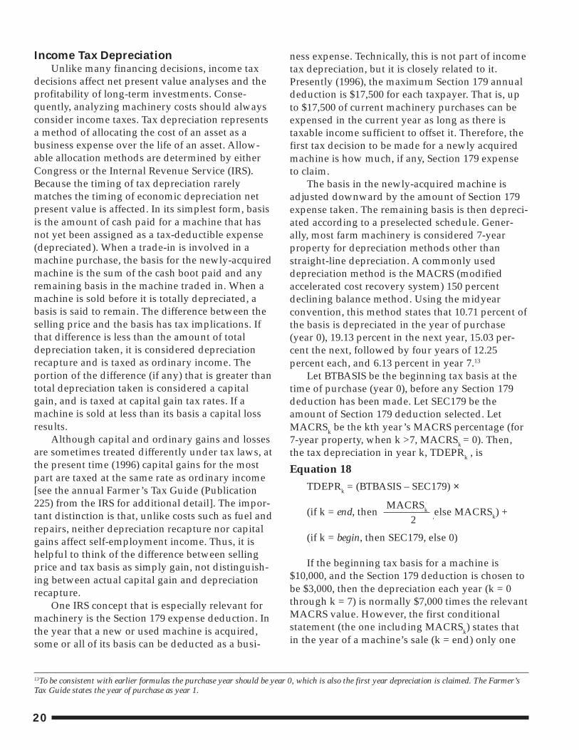
The formulas in this bulletin were used tocompute the cost per acre associated with a Case-IH combine with a 30 foot platform purchased newin 1996 for $150,000. Costs are compared acrossthree annual wheat harvesting acreages, 1,000,2,000, and 6,000; and across 20 trading regimes, at 1year through 20 years. Field efficiency and operat-ing speed from appropriate tables imply that 7.6

acres are covered per hour. Thus, the 1,000, 2,000,and 6,000 annual acreages are associated witharound 132, 263, and 789 annual machine hours,respectively. The first two usage levels would bemore typical of a farmer-owned combine, and thethird level of a custom harvester. Other assump-tions are: a bank loan rate of 0.10, which implies anafter tax cost of capital, COC, of 0.06; inflation rate,0.0245; marginal tax rate (T1), 0.2635; marginal taxrate (T2), 0.40; diesel fuel cost (1996), $0.90 pergallon; and labor cost (1996), $10 per hour. Section179 expensing deduction was 0 and remainingvalues were computed with Cross and Perryformulas (Equation 4).

Figure 9 depicts the pre-tax per-acre costs forthe combining example just described. Per-acrecosts are consistently lower for higher usage rates,regardless of how long the combine is owned.However, per-acre costs for the minimally usedmachine (1,000 acres) drop dramatically when themachine is held for more than one year. In thatcase, the farmer may want to hold the machine for20 years or more. For the mid-usage machine (2,000acres), cost per acre flattens out after 4 or 5 years,suggesting this may be a good time to trade–especially if timeliness costs were to be madeexplicit, which could easily offset the marginalreductions in costs associated with holding thecombine for more than 4 or 5 years. For the sup-posed custom harvester (6,000 acres), costs flattenout much more quickly, suggesting the machineshould be traded off in 2 years.

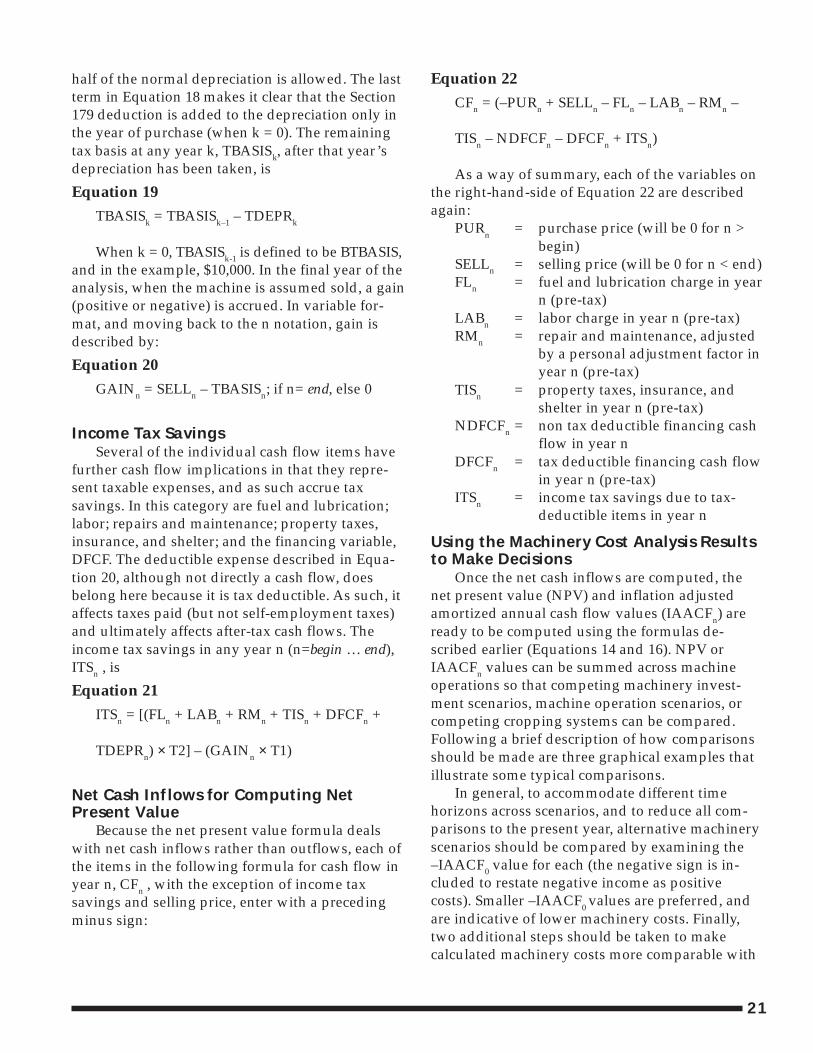
Example 2: Costs for a New Case-IHCombine across Three Inflation Rates

Figure 10 shows the costs associated with theCase-IH combine harvesting 2,000 acres per yearand at 3 different inflation rates: a) 0.0; b) 0.0245(the same rate used in the preceding example); andc) 0.0736 (3 times the rate used in the precedingexample). Because the cost of capital was fixed at0.06, (a) represents an increase in the real interestrate from the previous example and (c) represents adecrease. The increased incentives associated withdecreased real interest rates, both to purchase a newcombine and to trade more often, are readily seen.First, at any holding period length considered,higher inflation rates are associated with lower costsin 1996 pre-tax dollars. This means purchasing anew combine is more attractive with lower realinterest rates (here, through higher inflation rates).

Cost per Acre for a Case-IH Combine, at ThreeAnnual Usage Rates (1996 dollars, pre-tax)

Figure 9.

Dol

lars

Years Machine is Held

1000 Acres 2000 Acres6000 Acres

50

40

30

20

10

0201 3 4 5 6 7 8 92 10 11 12 13 14 15 16 17 18 19

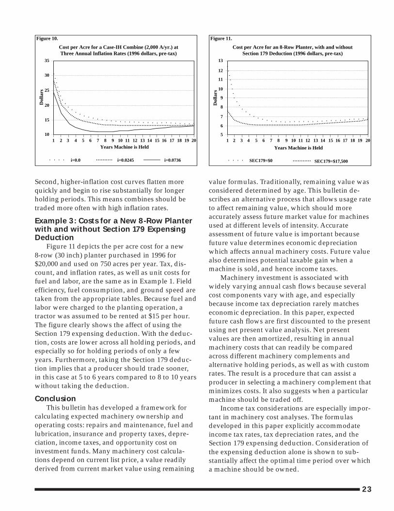
23

Second, higher-inflation cost curves flatten morequickly and begin to rise substantially for longerholding periods. This means combines should betraded more often with high inflation rates.

Example 3: Costs for a New 8-Row Planterwith and without Section 179 ExpensingDeduction

Figure 11 depicts the per acre cost for a new8-row (30 inch) planter purchased in 1996 for$20,000 and used on 750 acres per year. Tax, dis-count, and inflation rates, as well as unit costs forfuel and labor, are the same as in Example 1. Fieldefficiency, fuel consumption, and ground speed aretaken from the appropriate tables. Because fuel andlabor were charged to the planting operation, atractor was assumed to be rented at $15 per hour.The figure clearly shows the affect of using theSection 179 expensing deduction. With the deduc-tion, costs are lower across all holding periods, andespecially so for holding periods of only a fewyears. Furthermore, taking the Section 179 deduc-tion implies that a producer should trade sooner,in this case at 5 to 6 years compared to 8 to 10 yearswithout taking the deduction.

ConclusionThis bulletin has developed a framework for

calculating expected machinery ownership andoperating costs: repairs and maintenance, fuel andlubrication, insurance and property taxes, depre-ciation, income taxes, and opportunity cost oninvestment funds. Many machinery cost calcula-tions depend on current list price, a value readilyderived from current market value using remaining

value formulas. Traditionally, remaining value wasconsidered determined by age. This bulletin de-scribes an alternative process that allows usage rateto affect remaining value, which should moreaccurately assess future market value for machinesused at different levels of intensity. Accurateassessment of future value is important becausefuture value determines economic depreciationwhich affects annual machinery costs. Future valuealso determines potential taxable gain when amachine is sold, and hence income taxes.

Machinery investment is associated withwidely varying annual cash flows because severalcost components vary with age, and especiallybecause income tax depreciation rarely matcheseconomic depreciation. In this paper, expectedfuture cash flows are first discounted to the presentusing net present value analysis. Net presentvalues are then amortized, resulting in annualmachinery costs that can readily be comparedacross different machinery complements andalternative holding periods, as well as with customrates. The result is a procedure that can assist aproducer in selecting a machinery complement thatminimizes costs. It also suggests when a particularmachine should be traded off.

Income tax considerations are especially impor-tant in machinery cost analyses. The formulasdeveloped in this paper explicitly accommodateincome tax rates, tax depreciation rates, and theSection 179 expensing deduction. Consideration ofthe expensing deduction alone is shown to sub-stantially affect the optimal time period over whicha machine should be owned.

Cost per Acre for a Case-IH Combine (2,000 A/yr.) atThree Annual Inflation Rates (1996 dollars, pre-tax)

Figure 10.D

olla

rs

Years Machine is Held

i=0.0 i=0.0245 i=0.0736

35

30

25

20

15

10201 3 4 5 6 7 8 92 10 11 12 13 14 15 16 17 18 19

Cost per Acre for an 8-Row Planter, with and withoutSection 179 Deduction (1996 dollars, pre-tax)

Figure 11.

Dol

lars

Years Machine is Held

SEC179=$0 SEC179=$17,500

13

12

11

10

9

8

7

6

5201 3 4 5 6 7 8 92 10 11 12 13 14 15 16 17 18 19

24

Although financing decisions should typicallynot affect machinery decisions, financing formulashave been included so that alternative financingarrangements, such as leasing, or concessionaryloans, can be considered. Also, making explicit thefinancing cash flows should assist cash flow man-agement.

Because the formulas provided in this publica-tion can readily be developed in a computer spread-sheet, this bulletin should help producers makemachinery cost calculations, and ultimately theprofit maximizing decisions which follow. Thedevelopment of such a spreadsheet will enhanceunderstanding of the concepts presented. Further,those concepts are more important than the exactvalues falling out of the calculations. Finally, for-mula-based cost calculations should always bevalidated against personal experience. Whereexperience suggests calculations should be modi-fied, an understanding of the principles and math-ematics underlying the formulas will assist inmaking reasonable modifications.

ReferencesBowers, W. Machinery Replacement Strategies.

Moline, IL: Deere & Company, 1994.

Cross, T.L. and G.M. Perry. “DepreciationPatterns for Agricultural Machinery.” AmericanJournal of Agricultural Economics. 77(February,1995):194-204.

Farmer's Tax Guide, Publication 225. InternalRevenue Service, Department of the Treasury.Published annually.

Hot Line, Inc., Hot Line: Farm EquipmentGuide. Fort Dodge, Iowa.

KSU Farm Management Guides, Crops. De-partment of Agricultural Economics, Kansas StateUniversity.

Kansas Department of Agriculture, KansasAgricultural Statistics. Custom Rates.

Kastens, T.L., A.M. Featherstone, and A.W.Biere. “A Neural Network Primer for Economists.”Agricultural Financial Review. 55(1995):54-73.

Kansas State University Agricultural Experiment Station and Cooperative Extension Service

MF-2244 May 1997

It is the policy of Kansas State University Agricultural Experiment Station and Cooperative Extension Service that all persons shall have equal opportunityand access to its educational programs, services, activities, and materials without regard to race, color, religion, national origin, sex, age or disability. KansasState University is an equal opportunity organization. Issued in furtherance of Cooperative Extension Work, Acts of May 8 and June 30, 1914, as amended.Kansas State University, County Extension Councils, Extension Districts, and United States Department of Agriculture Cooperating, Marc A. Johnson,Director.File code: Farm Management 2-2

Brand names appearing in this publication are for product identification purposes only. No endorsement is intended,nor is criticism implied of similar products not mentioned.

Publications from Kansas State University are available on the World Wide Web at: http://www.oznet.ksu.edu

Contents of this publication may be freely reproduced for educational purposes. All other rights reserved. In each case, credit TerryKastens, Farm Machinery Operation Cost Calculations, Kansas State University, May 1997.