farm organization and values - open...
TRANSCRIPT

Description of the Salt River Project and impact ofwater rights on optimum farm organization and values
Item Type Thesis-Reproduction (electronic); text
Authors Ahmed, Muddathir Ali, 1935-
Publisher The University of Arizona.
Rights Copyright © is held by the author. Digital access to this materialis made possible by the University Libraries, University of Arizona.Further transmission, reproduction or presentation (such aspublic display or performance) of protected items is prohibitedexcept with permission of the author.
Download date 24/05/2018 21:11:42
Link to Item http://hdl.handle.net/10150/191465

DESCRIPTION OF THE SALT RIVER PROJECT AND
IMPACT OF WATER RIGHTS ON OPTIMUM
FARM ORGANIZATION AND VALUES
br
Muddathir All Ahmed
A Thesis Submitted to the Faculty of the
DEPARTMENT OF AGRICULTURAL ECONOMICS
In Partial Fulfillment of the RequirementsFor the Degree of
MASTER OF SCIENCE
In the Graduate College
THE UNIVERSITY OF ARIZONA
1965

STATEMENT BY AUTHOR
This thesis has been submitted in partial fulfillment ofrequirements for an advanced degree at The University of Arizonaand is deposited in the University Library to be made availableto borrowers under rules of the Library.
Brief quotations from this thesis are allowable withoutspecial permission, provided that accurate acknowledgment ofsource is made. Requests for permission for extended quotationfrom or reproduction of this manuscript in whole or in part maybe granted by the head of the major department or the Dean ofthe Graduate College when in his judgment the proposed use ofthe material is in the interests of scholarship. In all otherinstances, however, permission must be obtained from the author.
SIGNED: i c L
APPROVAL BY THESIS DIRECTOR
This thesis has been approved on the date shown below:
7 /tJy. // ,
AaronG. Nelson DateProfessor of Agricultural Economics

ACKNOWLEDGMENTS
The writer wishes to express his sincere appreciation and
thanks to the Sudan Government for granting him a scholarship to come
to the University of Arizona to pursue his graduate work.
The writer is deeply indebted to Dr. Aaron G. Nelson for his
guidance and encouragement during his course of study and for his
direction, assistance, helpful criticism and editorial comments con-
tributed during the preparation of the thesis.
The writer also gratefully acknowledges the constructive
comments and suggestions of Dr. Robert A. Young and extends his
sincere thanks to Drs. Maurice M. Kelso and Robert S. Firch for
their assistance.
To the Salt River Project personnel the writer extends his
appreciation for explaining and demonstrating operation of the Project
and for answering his questions during his study of the Project.
iii

TABLE OF CONTENTS
Page
LIST OF TABLES ......................... viiiLIST OF ILLUSTRATIONS . ................. xi
ABSTRACT . . . . ............xiiChapter
INTRODUCTION, . . , ..........1Description of the Salt River Project 1
Literature Review on the Problem 5
Objectives of the Study. , , 6
Procedure . , , , , 8
The Economic Model. ........, 10
Sources of Data . . . . . , , 17
NATURE, ORGANIZATION AND OPERATION OFTHE SALT RIVER PROJECT . . . . 20
Organization and Administration 20
Organization of the Association 22
Watershed Department 24
Irrigation Operation Department . . , 24
Irrigation Service Department . . , , , , 26
Engineering Department 29
iv

V
Chapter Page
Construction and Maintenance Department . . . . 31
PowerGeneration . . . ..............33The Water Supply 36
The Surface Water Supply 36
Rivers 39
Normal flow 39
Storage system and the stored water 39
The interworking of the storage system . . 45
The Underground Water Supply 45
Project pumps 45
Interworking between stored and pumpedwater 46
Private pumps 50
Water Agreements with Others Having Rights to Water 50
The Roosevelt Water Conservation District . . 50
The Salt River Indians 51
Phelps Dodge Copper Company at Morenci . . . 52
The City of Phoenix Domestic Water Contract . 52
The City of Phoenix "Water Gates" Contract . . 53
Buckeye Irrigation District 53
Roosevelt Irrigation District 54
Peninsula and Horowitz 55

vi
Chapter Page
Water Rights Within Project , . . . 55
Normal Flow Water Right . . . 56
Water Right to Stored and Developed Water, 58
Water Rights to Pumped Water , 59
Canal System . . 59
Water Transmission and Distribution ,,,,,,,. 62
III. EFFECT OF WATER RIGHTS ON OPTIMUM FARMORGANIZATION . . , . . . . . , 64
Water Situations , , , , , , , 64
Cropping Pattern. , , , , , , , . 66
Yields and Associated Inputs of Materials, , . . 68
Commodity Prices and Expenses , , . , , . 69
Commodity Prices . , , . , 69
Expenses . 71
Costs per unit of input in 1965 and 1975, 71
Variable costs of production in 1965 . , 73
Variable costs of production in 1975 . . . 79
Overhead costs. . . 87
Returns over Variable Costs . , , , , , . 90
Budget Analysis for Water Situations in 1965 and1975 ......... . . . . 92
Budgets for Water Situations in 1965 , . , , 93
Budget for water situation I , , 93

vii
Chapter Page
Budget for water situation II 96
Budget for water situation III 97
Budget for water situation IV, . ,.., 97
Discussion 97
Budgets for Water Situations in 1975 98
Budgets for water situation 1 99
Budgets for water situation II 105
Budgets for water situation III 106
Budgets for water situation IV 107
Comparison of Cropping Systems in 1965 and1975 108
Returns to and Indicated Value of Land in1965 and 1975 109
IV SUMMARY AND CONCLUSIONS 114
LITERATURE CITED 122

LIST OF TABLES
Table Page
Project Power Generating Plants 35
Total Operating Costs and Expenses Charged toIrrigation Water in the Salt River Project and theSubsidy Derived from Power in the Period 1961-1964. . 36
The Normal Flow of the Salt (including Tonto) andVerde Rivers by Months for the Period 1956-19 62 . . . 40
Characteristics of Storage Dams on the Salt and VerdeRivers 42
The Project Pumping by Month in 1959 47
Acre Feet of Water Produced for Project Use from theTwo Sources of Water and the Percentage of Ground-water to the Overall Total for the Period 1955-1963 . . 48
Four Water Right Situations and Estimated MaximumAcre Feet of Water Which a 360 Acre Farm canObtain from Each, Salt River Project 65
Yield Estimates per Acre for the Major Field Cropsin the Salt River Project for 1965 and 1975 Periods. . . 68
Summary of Materials Used per Acre in 1965 and 1975for Producing Crop Enterprises 70
Estimated Input Costs per Unit in 1965 and 1975,Salt River Project 71
Estimated Variable Costs per Acre, Other Than Waterand Interest on Variable Costs, for Specified Cropsin the SaltRiver Project, 1965 74
Estimated Variable Costs of Production per Acre forEach Crop with Each Water Source, the Salt RiverProject 1965 80
viii

i)<
Table Page
Estimated Variable Costs per Acre, Other Than Waterand Interest on Variable Costs for Specified Crops,The Salt River Project, 1975 ...............81
Estimated Variable Costs of Production per Acre forEach Crop with Each Water Source, The Salt RiverProject, 1975 86
Estimated Cash and Non-Cash Overhead Costs per Farmwith the Four Water Situations in the Salt River Project1965 and 1975 88
Gross Returns, Variable Costs and Returns overVariable Costs per Acre for Specified Crops withEach Water Source in the Salt River Project,l965and 1975 91
Ranking of Crops Relative to their Returns overVariable Costs per Acre with Each Water Source inthe Salt River Project, 1965 and 1975 . 92
Cropping Systems and Returns over Variable Costs forWater Situations I and II in 1965 94
Cropping Systems and Returns over Variable Costs forWater Situations III and IV ............... . 95
Cropping Systems and Returns over Variable Costs forVtTater Situation Tin 1975 100
Cropping Systems and Returns over Variable Costs forWater Situation II in 1975 ................101
Cropping System and Returns over Variable Costs forWater Situation III in 1975 ................102
23. Cropping Systems and Returns over Variable Costs forWater Situation IV in 1975 103

x
Table Page
24. Returns over Variable Costs, Cash and Non-CashOverhead Costs, Returns to Land and the IndicatedValue of Land with the Four Water Situations, TheSalt River Project 1965 and 1975 111

LIST OF ILLUSTRATIONS
Figure Page
Optimum production combination of andenterprises at four levels of resource inputs withvarying rate of substitution (hypothetical) 13
Optimum production combination of andenterprises at three levels of resource inputs withconstant rate of substitution (hypothetical) 15
Salt River Project organization 23
Organization of the Association 24
Organization of the Irrigation Service Department 2 7
Organization of the Engineering Department 30
Organization of the Construction and MaintenanceDepartment 32
Map of Arizona showing the Salt River Watershed Area . 38
Combined Reservoir capacity and water stored 44
The trends of total acre feet of water produced for Projectuse and the percentages of surface water and ground-water to total in the period 1955-1963 49
xi

ABSTRACT OF THESIS
DESCRIPTION OF THE SALT RIVER PROJECT AND
IMPACT OF WATER RIGHTS ON OPTIMUM
FARM ORGANIZATION AND VALUES
by
Muddathir All Ahmed
This study pertains to the Salt River Project in Central Arizona,
located in an arid area where precipitation averages only eight inches
annually. The Project provides water to land within its boundaries
according to water rights of each parcel, and produces electric power, the
revenue of which is used in part to subsidize irrigation. The objectives
of the study are: 1) to outline the organization and operation of the
Project and 2) to analyze the effect of water rights on farm organization
and land values.
The Project, comprised of Power District and Water Users'
Association, is controlled by a board of governors elected by the share-
holders. The administration consists of a general manager, two associ-
ate and three assistant general managers for the Power District and one
associate general manager for the Association. The latter has five de-
partments, watershed, irrigation operation, irrigation service, engineering
xii

xiii
and construction and maintenance, their function being to provide and de-
liver water to water right holders.
Water rights are of three types: right to normal flow with pri-
orities varying from 1869 to 1909, rights to stored and developed water and
rights to pump water. Some farmers also own private wells.
Using four typical water situations, a budget analysis was made
of a typical 360 acre farm, using estimated current (1965) and anticipated
future (1975) input-output relationships, and alternative acreage combi-
nations of crops. Under current conditions water rights probably have no
effect upon the cropping system but probably do affect land values. With
cost-price relationships and adoption of technology estimated for 1975
water rights would have an effect on both the cropping system and on land
values.

CHAPTER I
INTRODUCTION
When a visitor first comes to Tucson, his attention is quickly
attracted to its arid climate and desert vegetation. He will see xero-
phetic plants, mainly the cactus, and stipulate-leaved plants wherever
he goes in the mountain area. All Llriversu that one sees in the valleys
are nothing more than dry river beds. Yet, in spite of this, he reads that
the Arizona farmer leads the nation as far as returns per farm are con-
cerned, 1 and also that Arizona is an important cotton-producing state.
All these things seem to be conflicting. How can an arid place like
Arizona with rainfall rarely exceeding eight inches in most of the state
produce high farm income and be considered as a major cotton-producing
&ea? One soon learns that irrigation plays a vital role, and that irri-
gation districts are an integral part of the economy of the state.
1. Elmer L. Menzie, "Arizona Farm Income leads Nation,"Progressive Agriculture In Arizona, March-April, 1964, Vol. XVI, No. 2,College of Agriculture, University of Arizona, Tucson, p. 5.
"In 1962, realized net income per farm in Arizona was $18, 142
(net income includes interest on owned capital). The nearest competingstate was California with $8,476; the United States average is $3,414."
1

Description of the Salt River Project
This study pertains to the Salt River Project in Maricopa County,
in south central Arizona. Maricopa County is the major agricultural
county of the state, having 40 percent of all the irrigated land. The Salt
River Project includes a substantial portion of the Salt River Valley and
about 43 percent of the irrigated land in Maricopa County.2 The Salt
River Project (hereafter referred to as the Project, except where the full
name would add clarity) has an area of about 375 square miles or 240,000
acres. As of 1962, 165,575 acres were under cultivation, 65,000 acres
were in residential, commercial and industrial subdivisions, and the re-
maining 94,250 acres were in farmsteads, ditches and roads. Within its
boundaries are the eight incorporated communities of Phoenix, Mesa,
Tempe, Scottsdale, Chandler, Glendale, Peoria, and Tolleson.
The climate of this ares has favored the production of regular
field crops as well as those more intensively cultivated, such as citrus
and truck crops. In winter months, the average maximum temperature is
in the middle or upper fifties and readings above 60 degrees are not un-
common. Summer temperatures are among the highest recorded in the
United States. The average monthly temperature is above 80 degrees.
The frost-free period is approximately 300 days, which facilitates
2. United States Department of Commerce, Bureau of theCensus. United States Agriculture Census, Arizona State, 1959. Also,Salt River Project Crops Reporting, Salt River Project, Phoenix, 1959-1963.
2

3
production of a wide range of crops. The average dates of last killing
frost in spring vary between late January and early February, while those
of the first killing frost in autumn vary between late November and early
December,
Precipitation varies from year to year,, with an average of eight
inches in the Project area. In the mountainous area of the Salt River
watershed, precipitation is greater', with an average of 20 inches of pre-
cipitation, This watershed precipitation is important for the flow of the
rivers and supply of surface water. Winter precipitation is normally much
gentler but longer lasting than that of summer. It is associated with
storms that move into Arizona from the north Pacific Ocean.
Irrigation in the Salt River Valley is not new. Shadowy tracings
of canals over the valley are estimated to have existed since 200 B.C.
Because of climatic changes and variability of the water supply, these
old cultivators were compelled to abandon agriculture.
As early as 1869 new settlers came to the West and are referred
to in the American literature as the pioneers. At that time, the Salt River
Valley again enjoyed a certain degree of success through irrigation. Yet
the same risks of water shortage that faced agriculture in the pre-Christian
era remained. Proper water storage facilities were still lacking.
1961.3. Salt River Project, Major Facts in Brief. Phoenix, Arizona,

4
It was with the dedication of Theodore Roosevelt Dam in 1911
that the Project began to play an important role in the economy of the
valley. The years succeeding 1911 witnessed the completion of five more
dams. With these dams, the uncertainty of water supply that character-
ized the agriculture of earlier periods is no longer a problem facing the
farmer of the twentieth century. A dependable water supply has been
made available to project water users. The water supply has been aI-
lotted to each farmer according to the water rights each farm possesses.,
The continuity of agriculture year after year in the Project is
made possible through the successful operation of this project. How the
Project is able to meet its obligations of securing an adequate water
supply year after year and at low cost defines the important role it is
playing in the economy of the Salt River Valley and of Maricopa County.
The water supply is limited to two sources, viz, the surface water supp1'
primarily provided by the watershed area, and the underground water
supply provided by the underground water.
Agricultural activities are also undertaken by other irrigation
districts in the valley who also have some rights to the surface water and/
or the underground water. Because of heavy pumping by all agricultural
districts, the water table is declining year after year with the effect that
pumping costs per acre foot of water are also increasing. These restraints
on underground water and surface water make it more difficult for the
Project to secure an adequate water supply for its shareholders,

5
Net revenues involve returns and costs. In the Salt River Valley,
water costs are a factor affecting the progress of agriculture. Increases
in water costs naturally cause production costs to increase. When these
water costs continue to increase over time, the production costs will
also continue to increase and unless the gross returns are matched by
equal increases or more, the returns over the production costs will con-
tinue to decrease.
The apportionment of water supply to the various parcels of
land is done in line with the water rights each farm possesses. The
type of water rights (assessment, normal flow, etc.) vary from one parcel
of land to the other. Variations in type of rights involve also variation
in water costs. Pumped water is more costly than surface water, and
"excess" water and normal flow water are more costly than water from
assessment. Variations in water rights among farms may have an effect
on farm organization and operation. They may have an effect on farm
decision-making as to what crops to grow and how much, in order to
maximize farm returns from the water available to the farm.
Literature Review on the Problem
Very few studies have been made with regard to the important
role of the Project in agriculture and its operation in fulfilling this role.
The Project has published a small bulletin stating the major facts in

6
brief.4 This bulletin, however, does not go into the nature, operation,
and organization of the Project, factors which are believed to have a
bearing on water availability and cost. Other material may be found in
short articles in newspapers and magazines. This material does not
cover any one portion of the problem in detail. 5 As to the effect of water
rights on farm organization and operation and the impact of these water
rights on the cropping system, no analysis has ever been made.
Objectives of the Study
This study has two objectives: First, to investigate the nature,
organization, and operation of the Salt River Project and the different
water rights belonging to land in the Project. The supporting objectives
to this objective are:
To describe the nature, organization, and operation of the
Project.
To describe the different sources of water available to the
Project and the variability of supply from these sources.
To describe the methods and practices used by the Project in
Salt River Project, Major Facts in Brief, Salt River Project,Phoenix, Arizona, 1961.
Stephen C. Shadegg, The Phoenix Story, an Adventure inReclamation, Phoenix, Arizona.

7
order to maintain and make available water supply for agri-
cultural use.
To describe the water agreements between the Project and
other districts or parties having rights to water.
To describe the water rights within the Project and the
classification of these rights.
The second objective of this study is to analyze the impact of
water rights on farm organization. This objective is investigated at two
points in time, 1965 and 1975.
The choice of the two periods included in this study is made in
order to bring forward the effect of water rights in an immediate future
period, 1965, when there is little or no change and this effect ten years
in the future, 1975, when some changes in production, costs and returns
may take place. Moreover, analysis in these two periods will give the
farmer a basis for judgment when analyzing the future aspects of his farm
business.
Accomplishment of the above objective involves the following
aspects:
a. Determination of the production costs per acre for each crop
with each water source. (The term "water source" is intro-
duced to distinguish water from assessment, excess, normal
flow, project pump, or private pump (taken separately from
each other) from the term "water situation" which is defined

8
to mean a combination of these water sources at the farm
level.)
Determination of yields, commodity prices and gross returns
per acre for each crop.
Determination of returns over variable costs per acre for
each crop with each water source.
Determination of the most profitable crops for the area and
ranking them on the basis of their highest returns over
variable costs per acre with each water source.
Determination of the most profitable cropping system for
each water situation.
Determination of the returns to real estate in each water
situation. These are defined as the returns over and above
the variable costs, overhead cash costs and overhead non-
cash costs other than land.
Determination of the indicated value of land (from the income
approach) and noting the changes in this value if any, be-
tween the two periods chosen in this study.
Procedure
The procedure used in carrying out the first objective is to des-
cribe what has happened or what is happening. Description of the various

9
aspects of the Project pertaining to the availability of water, operation
and organization of the Project is done in fairly complete detail.
In carrying out the second objective, budget analysis was made
of a typical medium-sized commercial farm of 360 acres. Assuming
different water situations typical of the project, the analysis is made in
terms of the two periods, 1965, and 1975. Resources which are not
varied in the 1965 period are land, "assessment water'1, improvements,
machinery, and management. Water other than assessment is variable
because the farmer can buy any amount he wants within the limits pro-
vided by the water rights of his farm, This period, however, is long
enough to allow variation in the quantities of such resources as labor,
fuel and oil, repair and maintenance for the machinery, and raw materials
such as seeds, fertilizers, and insecticides.
In the 1975 period, factors of production were classified as
fixed and variable, the same as in the 1965 analysis. It was assumed
that farmers would be operating with a complement of fixed resources, in-
cluding machinery, similar to 1965. Adjustments were made in some of
the production, price and cost items as explained in detail in Chapter III
to account for anticipated relative changes over the decade.
The same calendars of operations for crop production are assumed
to prevail in each of the water situations. The operating costs however,
may differ depending on the type of water used in each water situation.

6. Earl 0. Heady, Economics of Aqricultural Production andResource Use. Prentice-Hall, Inc. , Englewood,Cliffs, New Jersey,1961.
10
Presently known technology is assumed for 1975. However, the
response of the farmer in 1975 may be greater than in 1965. More farmers
in 1975 may use the fertilizer programs and new varieties of hybrid al-
falfa, barley and sorghum which, as the agricultural specialists believe,
may increase yield.
The Economic Model
The theoretical framework for analysis of the impact of water
rights on the cropping system involves three basic relationships in pro-
duction economics. 6 These relationships are the factor-factor relation-
ships, the factor-product relationships, and the product-product
relationships. Factor-factor relationships are concerned with the rela-
tive amounts of two or more factors used to produce a given product.
These factors may be combined at different levels to produce the same
amount of product. The most efficient use is attained when their marginal
rate of substitutability is equal to the inverse ratio of their prices:
Xl = - x2x2
whereX1 means infinitesimal change in X1 andX2 means infinitesimal
change in X2.

11
X1 and X2 are two inputs. P and x2 are prices of the two
inputs X1 and X2, respectively.
Factor-product relationships involve the relationships between
resources used and the product which is produced. Again the equilibrium
point is reached when the additional output produced relative to the ad-
ditional units of resources used is equal to the inverse ratio of their
prices:
Ly Px1Ax
where Y is infinitesimal change in output, andX is infinitesimal
change in input associated withY.
Py and ' are prices of Y and X respectively.
Product-product relationships are concerned with allocation of a
given amount of resources among two or more enterprises. This assumes
that a given resource, or package of resources are held constant--iso-
resources--while different combinations of crops can be produced with
that given level of resources. The optimum allocation of given resources
between the enterprises can be made only if the choice criterion is known.
For farm profit maximizations, product price ratios provide the
choice indicator. Maximum profits are attained with costs or resources
fixed, when the marginal rate of substitution of products is inversely
7. Ibid., p. 239.

12
equal to the product price ratio:
= - Py2I
Fyi
(A1) (P1) = (Y2) (P2) II
whereY1 andY2 are infinitesimal changes in the production of enter-
prises and Y2, respectively.
Once the substitution and price ratios have been equated, the
following conditions of equal productivities are attained:
Equation II derived from equation I states that with resources
allocated to maximize profits, the marginal value product of a unit of
resource allocated to Y1 is equal to the marginal value product of a unit
of resource allocated to Y2. As long as the marginal rate of product sub-
stitutionY1/4y2 is less than the inverse price ratio P2/P11 profits can
be increased by substituting Y1 for Y2.
Optimum production combinations can be illustrated geometri-
cally by drawing iso-cost and iso-revenue curves on a production cost
surface. Figure 1 shows a production cost surface with varying rate of
substitution. The iso-cost curves indicate various combinations of the
two products Y1 and Y2 which can be produced with a given quantity of
resources. The iso-revenue lines indicate the combinations of two crops
which produce a constant revenue. The points of tangency of iso-cost

T
PRODUCTION OF
Figure 1. Optimum production combination of and Y2 enterprises atfour levels of resource inputs with varying rates of substi-tution (hypothetical),
ISO-REVENUE
ISO-COST
EXPANSION PATH
C4
R4
13

14
curves with iso-revenue curves indicate optimum combination of enter-
prises. At these points, the marginal rate of substituthbility of the two
crops is equal to the inverse of their prices ratio. However, these points
may not give the most profitable level of production--the most profitable
level of production as is indicated by the expansion path AB (Fig. 1), is
attained by climbing up the cost surface along the expansion path until
marginal revenue equals marginal cost. The expansion path is the line
connecting all points of tangency of iso-cost and iso-revenue. The opti-
mum combination of enterprises Y1 and Y2 for the given iso-resource C3
is OL of and OT of as given by the point of tangency of iso-cost C3
and iso-revenue R3. (See Figure 1..)
The above illustration assumes varying rates of substitution but
sometimes product-product relationships involve a constant rate of sub-
stitution. As the price ratio is the choice indicator, then whenever this
ratio is less than the marginal rate of substitutability between the two
crops, it will be most profitable to use all resources to produce the crop
that has the greater marginal rate of substitutability and low price ratios,
and leave the other crops (for example whenY1 = 4 and 2).3 yl 5
In Figure 2, the optimum levels of production are illustrated by the inter-
section of the iso-cost and the iso-revenue curves. When the iso-revenue
curve intersects two iso-cost curves at the two axes, then the optimum
level of production is given by the point where the iso-revenue intersects

T
Figu
re 2
,O
ptim
um p
rodu
ctio
n co
mbi
natio
ns o
fan
d Y
2 en
terp
rise
s at
thre
e le
vels
ofre
sour
ce in
puts
with
con
stan
t rat
e of
sub
stitu
tion
(hyp
othe
tical
),
PRO
DU
CT
ION
OF
Yl

16
the lowest of the two iso-cost curves. For example, in Figure 2, given
the iso-revenue R2 and iso-costs C2 and C3, the optimum level of pro-
duction is OL given by the intersection of R2 and C2.
When the inverse price ratio between two crops is the same as
the constant marginal rate of substitutability between these two crops,
the farmer is indifferent between producing all of one crop or producing
any combination of the two crops.
While the factor-factor and the factor-product relationships are
taken as given in this study for 19658 and are developed for l975 the
productproduct relationships provide the basis for analysis of the
second objective, i. e. the impact of water rights on farm organization.
In the budgetary analysis, it is assumed that the constant rate
of substitution relationships will prevail between the different crops.
Analysis of the prices indicate that the inverse price ratios prevailing
between the crops are different from the marginal rate of substitution
between these crops. It is assumed, however, that the farmer will not put
all his land in one crop if his goal is to maximize returns over a long
period of time. Growing all of one crop on a parcel of land is found to
deplete the soil and a point in time may be reached when this crop will no
They are already determined for a study (including area ofabove study) under preparation by Dr. Aaron G. Nelson, Professor of Agri-cultural Economics, University of Arizona.
They are developed in a similar manner to 1965.

10. Arizona Highway Department and others.
17
longer pay. A satisfactory rotation is therefore the practice of a good
farmer. Also because uncertainty characterizes agriculture--climatic
changes, pest infestation, uncertainty in commodity prices, etc.--and
because of the drive for an efficient use of his labor throughout the year,
the farmer is believed to adopt crop diversification. Moreover, insti-
tutional restrictions and water peak requirements prevent farmers from
putting all their land under one crop. Special attention has been given to
these restrictions when setting the budgets.
The above framework provides a conceptual basis for dealing
with any number of products. When large numbers of products are in-
volved, mathematical (algebraic) procedures may be used in place of geo-
metrical models.
Sources of Data
Data pertaining to the first part of this study were collected pri-
marily from the Salt River Project. The author spent part of the summer of
1963 studying the Project. He visited with Project personnel on the
various aspects of the Project. Most of the information was obtained first-
hand, directly from Project personnel. Other information was obtained
from the Bureau of Reclamation in Phoenix, from publications by some
writers interested in the Project'°, from project records and reports, and

18
from court decisions in cases involving the Project and others. Data
pertaining to the second objective and used in the 1965 budgetary analyses
were obtained from the Department of Agricultural Economics of the Uni-
versity of Arizona. These data include calendars of operations, costs
of production, commodity prices and yields. These data,however, were
supplemented by other data from offices of the United States Department
of Agriculture in Phoenix.
Yield estimates for 1975 are based on the judgment of specialists
12in the College of Agriculture of the University of Arizona. These judg-
ments indicate that the yields of all the crops under this study may in-
crease. Associated with these increases in yield are higher levels of
fertilizer applications.
Aaron G. Nelson, Costs and Returns for Major Field Cropsin Central Arizona by Size of Farm, Arizona Agricultural ExperimentStation Bulletin in preparation, 1965.
Lyman R. Amburgey, Robert E. Dennis, Aaron G. Nelsonand others.

13, U. S.D .A.,, Agricultural Statistics, U. S. GovernmentPrinting Office, Washington, D. C., 1963.
Natalie D. White and others, Annual Report on Ground-water in Arizona, Spring 1962 to Spring 1963. U, S, Geological Survey,Phoenix, Arizona, 1962. Also Alan P. Kleinman, The Cost of PumpingIrrigation Water in Central Arizona, Unpublished Ms. Thesis, Uni-versity of Arizona, Tucson, 1964.
U, S. D. A., Farm Real Estate Taxes, Recent Trends andDevelopments, A. R. 5. 43-130, 1960,
U. S. D. A,, Agricultural Price and Cost Projections forUse in Making Benefit and Cost Analysis of Land and Water ResourceProjects, Washington, D, C., 1957.
19
Data available indicate that the per unit costs of labor13, manage-
ment and groundwater14, and farm real estate taxes per acre15 may increase,
relative to other costs, in 1975 while the prices of cotton lint16 may fall
and those of cotton seed16 may rise, relativejy. (Discussion of above
per unit costs is given in Chapter III,) Except for these items, it was
assumed the same per unit costs, calendars of operations, and commodity
prices would prevail in 1975 as in 1965.

CHAPTER II
NATURE, ORGANIZATION AND OPERATIONOF THE SALT RIVER PROJECT
Organization and Administration
The Salt River Project is a nonprofit organization which incor-
porates the Salt River Valley Water Users' Association (SRV\ATLTA; hereafter
referred to as the Association) and the Salt River Project Agricultural
Improvement and Power District (hereafter referred to as the Power District),
both of which have identical boundaries. The Power District was formed
to secure the rights, privileges, exemptions and immunities granted to
public corporations or political sub-divisions for the Association lands.
Under a contract between the Association and the Power District all Associ-
ation properties have been transferred to the Power District. "The
Association continued to operate all of the properties as agent of the
Power District until 1949 when the contract was amended whereby the
Power District took over the project with the Association continuing to
operate the irrigation system as agent of the Power District." S.R.P.
(1961)1
1. Salt River Project, Major Facts in Brief, 1961, p. 20.
20

21
The Salt River Project2 is divided into 10 reservoir districts. At
the general elections the shareholders3 elect from each of the 10 districts
one governor for the Association board of governors, one director for the
Power District board of directors and three councilmen. At the same e-
lection and in addition to the above electees, a president and a vice
president are elected at large for the board of governors and the board of
directors. There are always two elections at the same time, one from the
Association side and the other from the Power District side. Thus while
a board of governors and a board of directors are elected, the two boards
have always been composed of the same individuals. For this reason and
for simplification the term Board will be used throughout the manuscript
when referring to these bodies.
To run for the office of president, vice president, governor,
director, or councilman an individual must be an owner of at least one
acre of land within the Project and a resident of the Project. "If he
should during his term of office cease to be such an owner or resident of
such Reservoir District, his office shall thereof become vacant." (Arti-
cles of Incorporation of SRVWUA, 1903, p. 11). The elector also must
be an owner of land. Each acre of land has one vote. The Association
The word 'project' is used whenever is meant the wholeorganization.
The word 'shareholders' includes those who own one or moreacres of land within the Project and who pay the "assessment" directly tothe project.

22
ejector has a maximum of 160 votes whereas the Power District elector can
cast as many votes as he has acres of land. Companies, corporations,
municipalities, and churches have no right to vote. Each shareholder as
to vote in person.
Figure 3 shows the general organization of the Project. The
Project has one general manager, one treasurer, one project secretary
and comptroller. All are appointed by the Board.
Working under the general manager are: one associate generai
manager for the Project Association, and two associate general managers
and three assistant general managers for the Power District. The associ-
ate general managers and the assistant general managers are selected by
the general manager but are approved and appointed by the Board. Under
the associate and assistant general managers for the Project Power Dis-
trict come the different departments of the Project Power Districts and
under the Associate general manager for the Water Users' Association
come the different departments of the Project Water Users' Association.
While no attempt is made to discuss the organization of the
Power District, the organization of the Project Water Users' Associ-
ation is hereafter briefly discussed.
Organization of the Association
There are five departments in the Association, each of which has
a different objective and function unique to itself yet all the five departments

TREASURER
BOARD OF GOVERNORS AND BOARD OF DIRECTORS
ASSOCIATE GENERALMANAGER
AS SI STANTGENERALMANAGER
ASSISTANTGE NERALMANAGER
GENERAL MANAGER
ASSOCIATE GENERALMANAGER
AGRICULTURAL IMPROVEMENT AND POWER DISTRICT
Figure 3. Salt River Project Organization
ASSISTANTGENERALMANAGER
23
PROJECTSECRETARY 1COMPTROLLER
ASSOCIATE GENERALMANAGER
WATERUSERS'ASSOCIATION
Source: Reference Manual of Association operation, Salt River Project, 1962
PRE SIDE NT VICE PRESIDENT

are Important key factors and all vital to successful operation. These
departments, portrayed in Figure 4, are discussed below.
ASSOCIATE GENERAL MANAGER
Figure 4. OrganizatIon of the Association.
Watershed Department
The objectives of this department are to observe, record, and
take necessary action for the protection of the water supply from uses by
others not entitled to it, and for the conserving of this water supply for
the project storage system. It conducts the annual survey of watershed
snow-pack and provides an estimate (forecast) of expected water yield to
the river system.
The Watershed Department participates with other agencies in a
watershed research program whose goals are the stabilization and increase
of natural resources from the watershed area.
Irrigation Operation Department
The Irrigation Operation Department Is comprised of transmission
and communication division and the water distribution division.
The primary objective of this department is to deliver, with a
minimum of loss, the stored and developed water to the land within the
24
Watershed Irrigation Irrigation Engineering ConstructionDepartment Operation Service Department & Maintenance
Department Department Department

25
project on demand of the shareholders. To achieve this objective it per-
forms the following functions:
Receiving and recording water orders from shareholders.
Requesting release of water from reservoirs and transmitting
it to canal system.
Operating deep well pumps.
Coordinating dry-ups in project's laterals and canals to ac-
commodate private construtionsuchas installing an underground cable
across the lateral.
Delivering water to users on request.
Completing charge cards and submitting them to machine
accounting.
Requesting needed construction and maintenance.
Maintaining public relations by answering and correcting
complaints from users and the general public.
Patrolling the project when storms occur and disposing of
storm water.
Performing studies on work load, water demand and related
undertakings. The objective of these studies is to improve the services
of water distribution division to the shareholders.
Directing tours with foreign-visitors over the project.

26
Irrigation Service Department
The Irrigation Service Department consists of two divisions, the
accounting and collection division and the subdivision divisibn (Figure 5).
Each of these divisions has a number of sections performing different
duties. The accounting and collection division consists of the transfer
journal section, the plat and escrow section, bookkeeping section, and
customer service section.
The subdivision division consists of three sections: scheduling
section, subdivision irrigation section, and clerical section.
The primary objective of the Irrigation Service Department is to
properly administer the water rights of all land within the boundary of the
project.
The accounting and collection division provides the proper ac-
counting and collection of all revenues from the delivery and sale of
water for both irrigation and municipal domestic purposes. The ob-
jectives of the sections of this division are:
The transfer journal section is to properly process new
shareholder accounts.
The plat and escrow section is to properly maintain plats
for all sections within the exterior boundary of the project and daily es-
crow service to various title companies.
The bookkeeping section collects and accounts for all
revenues received for farm and residential irrigation, and for water
delivered to municipalities.

AC
CO
UN
TIN
G A
ND
CO
LL
EC
TIO
ND
IVIS
ION
ISU
PER
INT
EN
DE
NT
I
Figu
re 5
,O
rgan
izat
ion
of th
e Ir
riga
tion
Serv
ice
Dep
artm
ent
Sour
ce: R
efer
ence
Man
ual o
f A
ssoc
iatio
n O
pera
tion,
Salt
Riv
er P
roje
ct, 1
962,
,
SUB
DIV
ISIO
ND
IVIS
ION
TR
AN
SFE
RFL
AT
AN
DB
OO
KK
EE
PIN
GC
UST
OM
ER
SCH
ED
UL
ING
SUB
DIV
ISIO
NC
LE
RIC
AL
JOU
RN
AL
ESC
RO
WSE
CT
ION
SER
VIC
ESE
CT
I O
NIR
RIG
AT
ION
SEC
TIO
N
SEC
TIO
NSE
CT
ION
SEC
TIO
NC
OO
RD
INA
TO
R

Page Missingin Original
Volume

29
4. The customer service section processes service complaints
and responds to Inquiries and requests for service made by shareholders.
The objective of the subdivision division is to serve the
urbanized or subdivided residential areas of the project with the most
modern efficient type of flood irrigation service. It reports and accounts
for all water in the project. Part of the irrigation service functions is to
compile data that willaid in increasing the efficiency of deliveries to
users and the conservation of water.
Engineering Department
The Engineering Department consists of an administrative body--
office coordinator, administrative assistant, irrigation consultant and
operation coordinator, and of a technical body--civil engineering di-
vision and ground water division. Figure 6 shows the different sections
under each division.
The objective of the Engineering Department is to provide the
engineering and technical skills in construction, maintenance and
research for the irrigation transmission, distribution and groundwater
system, to maintain proper efficiency of water delivery to the share-
holders of the Project. The Association Engineering Department has the
following functions:
1. It provides engineering services for construction and
maintenance purposes pertaining to the irrigation transmission,

SUR
VE
YSE
CT
ION
CIV
ILE
NG
IWE
ER
ING
DIV
ISIO
N
DR
AFT
ING
SEC
TIO
ND
ESI
GN
AN
DIN
S FE
CT
IO
NSE
CT
ION
Figu
re 6
.O
rgan
izat
ion
of E
ngin
eeri
ng D
epar
tmen
t.
Sour
ce: R
efer
ence
Man
ual o
f A
ssoc
iatio
n O
pera
tion,
Sal
t Riv
er P
roje
ct,
1962
.
ASS
IST
AN
T C
HIE
FE
NG
INE
ER
(
GR
OU
ND
WA
TE
RD
IVIS
ION
LA
BO
RA
TO
RPL
AN
NIN
G &
HY
DR
OG
RA
PHIC
C &
M )
ESI
GN
&SE
CT
ION
DE
VE
LO
PME
NT
SEC
TIO
NSE
CT
IOT
EST
ING
I
SEC
TIO
NSE
CT
ION
J
OFF
ICE
AD
MIN
IST
RA
TIV
EIR
RIG
AT
I O
NO
PER
AT
ION
S
CO
OR
DIN
AT
OR
ASS
IST
AN
TC
ON
SUL
TA
NT
CO
NSU
LT
AN
T

31
distribution and division system. This is the responsibility of the civil
engineering division.
It provides engineering services in hydrography and chemistry
pertaining to the operation of the irrigation and electric hydro-generation
system. It constructs, maintains and operates facilities pertaining to the
ground water production system; operates and maintains sand dredging
equipment at Granite Reef Diversion Dam and provides engineering plan-
ning and development pertaining to the entire irrigation system. This is
the responsibility of the groundwater division.
It helps plan and coordinate the irrigation engineering and
construction functions and liaison between the Project and municipalities.
It provides technical service pertaining to irrigation prob-
lems for the engineering department, shareholders and others.
Construction and Maintenance Department
The Construction and Maintenance Department consists of two
construction and maintenance headquarters and a field engineer. Under
the above two headquarters function the six sections shown in Figure 7.
The objective of the Construction and Maintenance Department is
to maintain the irrigation facilities in a condition that will permit eco-
nomical and efficient operation of the system. It is responsible for
providing construction and maintenance pertaining to the irrigation trans-
mission, distribution, and diversion system. It coordinates and plans

SUPE
RIN
TE
ND
EN
T
Figu
re 7
.O
rgan
izat
ion
of C
onst
ruct
ion
and
Mai
nten
ance
Dep
artm
ent.
Sour
ce: R
efer
ence
Man
ual o
f A
ssoc
iatio
n O
pera
tion,
Sal
t Riv
er P
roje
ct, 1
962.
PHO
EN
IX A
ND
SOU
TH
ER
NE
AST
ER
NW
EE
DA
RIZ
ON
AG
RkN
DL
EH
IC
ON
STR
UC
TIO
NC
ON
STR
UC
TIO
NC
ON
TR
OL
CO
NST
RU
CT
ION
CO
NST
RU
CT
ION
CO
NST
RU
CT
ION
AR
EA
AR
EA
SEC
TIO
NA
RE
AA
RE
AA
RE
A
SOU
TH
SID
EW
AR
EH
OU
SEN
OR
TH
SID
EFI
EL
D
HE
AD
QU
AR
TE
RS
SEC
TIO
NH
EA
DQ
UA
RT
ER
SE
NG
INE
ER

4. Salt River Project Annual Report, 1958, p. 5.
33
man-power and equipment used by north side and south side headquarters.
It also evaluates weed control materials such as herbicides, selective
weed killers, and administers the weed control program. It recommends
Improvements or replacements of existing construction facilities. It also
improves existing construction and maintenance methods.
Power Generation
"The future of water supply in the Salt River Valley will depend
on continuing the partnership between these essential elements--water
and electric power."
"But behind all this success stands the reclamation principle:
the development of water resources financed by using money derived from
the production and sale of electric energy.
These two quotations from the president of the Project, indicate
the importance of power in the availability of water supply at low costs.
It was in 1937 when the Project organized the Project Agricultural Improve-
ment and Power District, a political subdivision of the State of Arizona
coexistive with the Salt River Valley Water Users' Association. In 1949
the Power District assumed the operation of the electrical and generating
systems.
In the early twenties there were two private utility companies
serving areas in central Arizona. These private utility companies signed

34
an agreement with the Salt River Project setting forth the boundaries and
outlines for the areas where the project would assume responsibility for
supplying power. The agreement was amended several times.
Population of central Arizona increased tremendously beginning
in 1945 and pushed new subdivisions into what formerly had been operating
farm land. This increased the responsibility of the project in meeting
the demand for electric power in its boundaries set by the above-
mentioned agreement. In 1940 the Project built its first steam generating
unit at Cross-Cut having a generating capacity of 7,500 kw. Because of
the continuous increase in population within the Project, the Project con-
tinued installing steam electric plants, the latest of which was built in
1961. A summary of the Project power generating plants is given in
Table 1.
Energy production increased from 829,539,000 kwh. in 1950 to
2,891,964,000 kwh. in 19626--an increase of over two billion kwh. The
Project Power is sold at both wholesale and retail, In 1960 the wholesale
distribution amounted to 11 percent while the retail distribution amounted to
89 percent. Revenue received from power sale in 1960 amounted to
$38,667,313.00.
W. Brandon Glenn, Historical Documents Pertaininq to PowerContracts and Agreements of the Salt River Project, 1961, p. 36.
The relationship between the generating capacity given in kw.and the production given in kwh. is that Production (kwh.) = GeneratingCapacity X No. of hours operated at that capacity.

35
From the farmer's point of view the important role that the Project's
power system plays is providing low cost water for its shareholders. At
the same time power revenue is used in meeting the annual maturity of
long term debt and interest. This debt is the result of financing the
different storage and power facilities of the Project through borrowing from
the Federal Government and through the sale of bonds.
In examining the Project' s annual statements of income from irri-
gation operation one finds a net operating deficit. This deficit is planned
each year in the process of budgeting the year's activities. It represents
the amount of money which will be available for water cost subsidy from
power revenue for that year. In this way benefits from power revenue are
passed directly to all water users including residential home owners.
Table 2 gives the total operating costs and expenses of water, and the
Table 1. Project Power Generating PlantsNature of Where Yr.
Power Generated Location Cons.GeneratingCapacity
No. ofCustomers
Hydroelectric Roosevelt Dam 80 mi. from 1911 19,247 kw.Phoenix
Hydroelectric Horse Mesa 65 mi. ' 1927 29,982 kw. 45-1921Hydroelectric Mormon Flat 51 mi. " 1925 6,997Hydroelectric Stewart Mt. 41 mi. 1930 10,384Thermal Elec. Cross Cut Cross Cut 1940 7,500Thermal Elec. Kyrene Kyrene 1952 30,000 " 8,000-1941Thermal Elec. Kyrene Kyre ne 1954 60,000Thermal Elec. Agua Fria Agua Fria 1957 100,000Thermal Elec. Agua Fria Agua Fria 1958 100,000Thermal Elec. Agua Fria Agua Fria 1961 175,000 " 97,975
120,000-1963

amount of subsidy derived from power for the period 1961-1964. Note
that the subsidy accounts for an average of 60 percent of the total
operating costs and expenses of water.
Table 2. Total Operating Costs and Expenses Charged to Irrigation Waterin the Salt River Project and the Subsidy Derived from Power inthe Period 1961-1964.
36
Source: Salt River Project Annual Reports from 196 1-1964.
The Water Supply
There are two sources of water supply in the Project, the surface
water supply and the underground water supply.
The Surface Water Supply
The surface water supply comes primarily from the watershed area.
This area constitutes an entire drainage area of 8,300,000 acres, located
in the mountainous areas of central Arizona. Figure 8 shows the State of
Arizona, watershed area, principal stream and storage dams. Of the entire
Total OperatingYear Costs and Expenses
Subsidy Derivedfrom Power
Percentage of Subsidyto Total Costs
1961 $ 9,596,000 $5,700,000 59.39%
1962 8,445,898 4,875,181 57.72
1963 8,657,653 5,175,491 59.77
1964 10,419,974 6,646,147 63.78
Average 9,279,881 5,599,204 60.34

37
drainage area 7,500,000 acres are above the dams and out of this only
2,500,000 acres are covered by snow in the winter season. Elevations
range from 1,325 feet above sea level to more than 11,000 feet. Above
elevation 4,000 feet, snowfall prevails during winter. Precipitation in-
creases generally with elevation. In the lower areas precipitation is in
the order of nine inches while at points in the high mountain area, pre-
cipitation falling upon the area above the dame is 20 inches, equivalent
to about 12,000,000 acre feet of water, Of this amount, 2.08 inches or
1,241,800 acre feet is accounted for annually by measurement at stream
gauging stations. The difference (17.9211) or 10, 758,200 acre feet of
water represent the amount of potential water supply which is used or
lost on watershed areas above reservoirs. Factors which contribute to
the disposition of precipitation in watershed areas above dams and to
resulting low stream flow are:
The interception, use and transpiration of water by natural
vegetation.
Evaporation from wet ground and snow.
Evaporation from stream channels and,
Diversion for agricultural and other upstream benefits.
7. George W. Barr and others, Recovering Rainfall; More Waterfor Irriqation, 1957.

z
0
IL
z
a
nO
Puma
C
A P A C H E
s oi-
' I rI..': 0FlooU
L
Iatershd boundry
',Y AV e
rjVoWe / .)
I
Pis
j i' .1
-I
I
MeNoryb JYOiW9 \I
Is
ARIZOrA WATERSHED PROGRAM000ppro 1109
Arizona Stole Land Deportment Water DivisionSalt River Volley Waler User, Association
Univartiry of Ariz000PHOENIX ARIZONA
ccr
U T
JR
P
rlvrenco -
I N
\sa
- \,-
NAVAJO
38
,1,
l' .1
n\ 'J GREENEjI
JG AH:
\ li
M A/ / \ I
Tvusnn,i
Brnaon I
MAP OF THE I / )l C 0 C H t S S
STATE OF ARIZONA('
PRINCIPAL STREAMS SYSTEM SNTCRUZI -\w/rH M N' I
OUTLINE OF SALTANO VERDE RIVER SAS/N5 and Damsx C 0
Figure 8. Map of Arizona showing the Salt RiverWatershed Area.
PLATE I
HA

Rivers
Water from the watershed area is carried by three rivers; the
Salt River, the Tonto River, and the Verde River. The Salt River and the
Tonto River flow into the Salt reservoir system (see below). These two
rivers are referred to hereafter as the Salt System. The Verde on the other
hand flows into Horseshoe and Bartlett Dams.
Normal flow
The normal flow of the rivers varies from river to river, from year
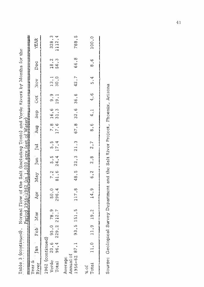
to year, and within the year. Table 3 gives the flow of the two systems
by months from 1956 to 1962. The table shows that the total amount
carried by the Salt System in any one year was greater than that carried by
the Verde River. The overall amount of water carried by both rivers also
varies from month to month within the year and from year to year.
The average annual flow of the two rivers for the period 1956 to
1962 was 788,500 acre feet (see Table 3). Note that normal flow in winter
and spring months is more than three quarters of the annual normal flow of
the two rivers. However, more than 40 percent of the total stream flow is
received during the winter months.
The storage system and the stored water
Water carried by the three rivers is stored in six reservoirs, four
on the Salt River and two on the Verde River. One diversion dam, Granite
Reef Diversion Dam, is located on the Salt River just below its confluence
39

Tab
le 3
,N
orm
al F
low
of
the
Salt
(inc
ludi
ng T
onto
) an
d V
erde
Riv
ers
by M
qths
for
the
Peri
od 1
956-
1962
in 1
000
acr
e fe
et o
f W
ater
Yea
r &
Riv
erJa
nFe
bM
arA
prM
ayJu
nJu
lA
ugSe
pO
ctN
ovD
ecY
EA
R
1956
Salt
15.4
26.8
47,7
39.8
23.4
7.2
9.3
12.4
6.5.
9.0
10.0
15.0
222.
5V
erde
15.4
14.0
12.6
11.0
7.2
5.2
12.6
11.6
5.9
11.2
13.1
17.4
137.
2T
otal
30.8
40.8
60,3
50.8
30.6
12.4
21.9
24.0
12.4
20.2
23.1
32.4
359.
719
57Sa
lt10
7.1
76.6
54.2
38.9
32.5
19.7
12.2
68.8
21.3
5.7
7.8
8.4
453.
2V
erde
83.0
124.
336
.210
.412
.410
.411
.919
.88.
19.
712
.514
.235
2.9
Tot
al19
0.1
200.
990
.449
.344
.931
.124
.188
.629
.415
.420
.322
.680
6.1
1958
Salt
12.5
50.0
241.
625
0.4
114.
424
.89.
320
.4 4
2.2
16.6
27.4
16.4
826.
0V
erde
14.3
50.0
165.
370
,39,
67.
74.
615
.636
.012
,857
.916
.646
0.7
Tot
al26
.810
0.0
406.
932
0.7
124.
032
.513
.936
.078
.229
.485
.333
.012
86.7
1959
Salt
12.2
13.5
16.0
15.4
8.2
4.7
1.6
97.0
14.3
44.0
14.9
13.8
255.
6V
erde
13.9
21.0
20.3
10.1
8.2
5.6
14.0
33,6
7.8
16.5
14.5
14.7
182.
2T
otal
26.1
34,5
36,3
25,5
16.4
10.3
15,6
130.
622
,161
.529
.428
.543
6.8
1960
Salt
219.
870
.221
4.5
102.
443
,517
.68.
511
.68.
856
.986
.922
7.1
1067
.8V
erde
52.8
23.7
115.
214
.69.
56.
55.
510
.714
.139
.318
.784
.139
4.7
Tot
al27
2.6
93.9
329,
711
7.0
53.0
24.1
14.0
22.3
22.9
96.2
105.
631
1.2
1462
.519
61Sa
lt12
.211
.523
.134
.312
.56.
68.
719
.819
.516
.012
.611
.918
8.7
Ver
de13
.812
.514
.224
.57.
55.
18.
216
.520
.213
.813
.614
.216
4.1
Tot
al25
,024
.037
.358
.819
.011
.716
.936
.339
.729
.826
.226
.135
2.8
1962
Salt
75.8
134
.213
3.8
246.
474
.418
.911
.99.
814
.79.
216
.938
.178
4.1
Tab
le 3
(co
ntin
ued)
.N
orm
al F
low
of
the
Salt
(inc
ludi
ng T
onto
) an
d V
erde
Riv
ers
by M
onth
s fo
r th
ePe
riod
195
6-19
62 in
1 0
00 a
cre
feet
of
Wat
er
Sour
ce: G
eolo
gica
l Sur
vey
Dep
artm
ent a
nd th
e Sa
lt R
iver
Pro
ject
, Pho
enix
, Ari
zona
Yea
r &
Riv
erJa
nFe
bM
arA
prM
ayJu
nJu
lA
üSe
pO
ctN
ovD
ecY
EA
R
1962
(co
ntin
ued)
Ver
de20
.695
.078
.950
.07.
25,
55.
57.
816
.69.
913
.118
.232
8.3
Tot
al96
.422
9.2
212.
729
6.4
81.6
24.4
17.4
17.6
31.3
19.1
30.0
56.3
1112
.4
Ave
rage
Ann
ual o
f19
56-6
2 87
.193
.5 1
51.5
117.
848
.522
,321
.367
.832
.636
.642
.766
.878
8.5
%of
Tot
al11
.0,
11.9
192
14.9
6,2
2.8
2.7
8.6
4.1
4.6
5.4
8.6
100.
0

42
with the Verde. This dam has limited storage capacity, its primary
function being to divert water released for agricultural use from the six
dams into the Project north and south canals, A summary of selected
information related to the storage system is given in Table 4.
Source: Salt River Project, Major Facts in Brief, 1961.
Table 4. Characteristics of Storage Dams on the Salt and Verde Rivers.
Location Water(Distance Holding Hydro-From Ht. Length Capacity electric
River and Phoenix in in in Ac. Year GeneratingDam in Miles) Ft. Feet Feet Built Capacity
SALT RIVER
Roosevelt 80 280 723 1,381,580 1905-11 Yes
Horse Mesa 65 300 660 245,138 1924-27 Yes
Mormon Flat 51 224 380 57,852 1923-25 Yes
StewartMountain 41 207 1,260 69,765 1928-30 Yes
VERDE RIVER
Horse Shoe 58 60 1,500 142,830 1944-46 None
Bartlett 46 283 800 179,548 1936-39 None
At the Confluxof Salt andVerde Rivers
Granite Reef DivertDiversion Dam 32 29 1,000 water 1906-08 None
43
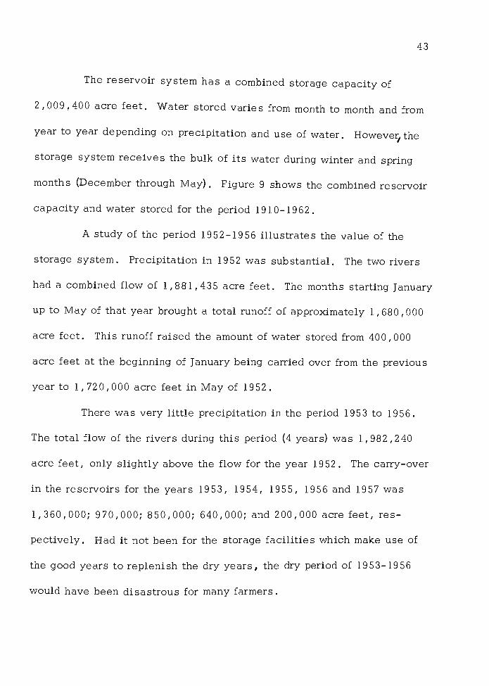
The reservoir system has a combined storage capacity of
2,009,400 acre feet. Water stored varies from month to month and from
year to year depending on precipitation and use of water. Howeve5,the
storage system receives the bulk of its water during winter and spring
months (December through May). Figure 9 shows the combined reservoir
capacity and water stored for the period 1910-1962.
A study of the period 1952-1956 illustrates the value of the
storage system. Precipitation in 1952 was substantial. The two rivers
had a combined flow of 1,881,435 acre feet. The months starting January
up to May of that year brought a total runoff of approximately 1,680,000
acre feet. This runoff raised the amount of water stored from 400,000
acre feet at the beginning of January being carried over from the previous
year to 1,720,000 acre feet in May of 1952.
There was very little precipitation in the period 1953 to 1956.
The total flow of the rivers during this period (4 years) was 1,982,240
acre feet, only slightly above the flow for the year 1952. The carry-over
in the reservoirs for the years 1953, 1954, 1955, 1956 and 1957 was
1,360,000; 970,000; 850,000; 640,000; and 200,000 acre feet, res-
pectively. Had it not been for the storage facilities which mae use of
the good years to replenish the dry years, the dry period of 1953-19 56
would have been disastrous for many farmers.

Page Missingin Original
Volume

45
The thterworking of the storage system
The procedure adopted in operating the storage system is to lower
the Verde system to a predetermined quantity to make certain of sufficient
storage capacity for any spring runoff. Having done that, water is then
demanded from Stewart Mountain Dam on the Salt System. This dam is
the lowest dam on the Salt Reservoir System. As water is released from
this dam, it passes through hydroelectric generating equipment and elec-
tricity is developed. In the meantime water is being released from the
dam above to replenish the water released from the reservoir below, and
as it does so electricity is generated. This process goes through all four
hydroelectric plants on the Salt System to keep the three downstream
reservoirs at maximum operating level.
The Underground Water Supply
Project pumps
Underground water is the other source of water supply in the
Project. Pumping of water started first as a result of the high water table
problem in the western part of the Project prior to and during the First
World War. Water was then pumped into the river. At that time the
Project entered into a contract for 99 years with the Roosevelt Irrigation
District (RID) to pump water within the Project boundaries (now amended).
But in the late 1920's and the 1930's, the Project faced draught and under-
ground water was badly needed to supplement stored water. The Project

46
began drilling wells to supplement surface water and by 1962 the Project
had 246 pumps. These pumps contributed each year 500,000 acre feet of
underground water. They are fairly evenly distributed all over the Project
and are installed near the canals to discharge the pumped water into the
Project canal system. The average pump size is 250 hp. The summer
months are the months of heavy pumping. Table 5 shows the amount of
water in acre feet that was pumped in each month of 1959. The amount
of pumped water varies inversely with the amount of runoff and stored
water in the dams.
Because of heavy pumping, the water table continued to drop
annually. 8 The drop in water table varies from one area to the other. The
annual report on ground water in Arizona, spring 1962 to spring 1963,
shows that the decline in water in the Project area ranged between 20
feet to 40 feet for the 5-year period 1958-1963. An average annual decline
of six feet is believed to be the rule. This continuous decline in water
table has a direct effect on costs of pumping due to the increase in lift.
Also because of the above fact the Project drills annually about six
replacement wells.
Interworking between stored and pumped water
Pumping during the heavy flow of rivers in winter and spring
months is less than during the summer months. In summer months because
8. Natalie White and others, Annual Report on Groundwater inArizona, Spring, 1962-Spring 1963, U. S. Geological Survey.

Table 5. The Project Pumping by Months in 1959. (Quantities in acrefeet.)
47
of the great demand for water by crops and because the flow of the rivers
is less than that of winter and spring, heavy pumping takes place. During
the summer months pumps work continuously for 24 hours per day. Table 6
gives the total acre feet of water produced for Project use from surface
water and from groundwatr sources and the relative percentages of these
Month North Side South Side Total
A B A/B
January 13,364 14,081 27,445
February 8,943 13,869 22,812
March 22,010 30,808 52,818
April 19,462 29,526 48,988
May 19,640 30,588 50,228
June 22,463 28,133 50,596
July 22,974 29,748 52,722
August 17,158 26,926 44,084
September 19,527 28,168 47,695
October 12,022 21,645 33,667
November 7,034 6,428 13,462
December 4,865 10,026 14,891
Total 189,462 269,946 459,408
Source: Salt River Hydrographic Section.

48
two sources to the total for the period 19 55-1963. Figure 10 indicates
that while the total acre feet of water produced for Project use is fairly
constant the surface water supply and the groundwater supply are in-
versely proportional to each other.
Table 6. Acre Feet of Water Produced for Project Jse from the Two Sourcesof Water and the Percentage of Groundwater to the Overall Totalfor the Period 1955-1963.
a. Note that the figures given here and in Table 5 for 1959 arenot the same, The figures were taken from different sources.
YearSurface Ground-Water water Total
Percentaqe of total waterSurface water:Groundwater
1955 600,007 467,619 l,07,626 56.2 43.8
1956 634,779 517,469 1,152,248 55.1 44.9
1957 528,417 461,461 989,878 53.4 46.6
1958 591,729 432,106 1,023,835 57.8 42.2
1959a 552,142 462,090 1,014,232 54.4 45.6
1960 719,892 352,747 1,072,639 67.1 32.9
1961 553,544 497,205 1,050,749 52.7 47.3
1962 727,404 403,521 1,130,925 64.3 35.7
1963 692,153 403,874 1,096,027 63.2 36.8
Total 5,600,067 3,998,092 9,598,159
Average 622,230 444,322 1,066,552 58.3 41.7
Source: Salt River Project Annual Reports for the period 1955-1963.

600-/0
500//0
400//0
300//0
I I I
Percentage of surface waterto total
Percentage of groundwater to total- -
- -
Total water produced forProject use
//
/''
49
1955 56 57 58 59 60 61 62 63
Figure 10. The trends of total acre feet of water produced for Project useand the percentages of surface water and groundwater to totalin the period 1955-1963.
a. Figures are in thousands of acre feet of water.
130 0a
(ac.. ft).
120 0a
(ac ft)
1 100a
(ac ft)
l000a(ac ft)
900a(ac ft)

50
Private pumps
Some farmers in the Project have their own private pumps to
supplement Project water. The number of these wells is believed to be
more than 400. Since 1956 no records have been kept for private wells
in the Project. The average annual amount of water recorded in the
period 1946-1956 was about 220,000 acre feet. There was little fluctu-
ation from year to year. Current data regarding private wells are lacking
and an economic study including these private wells may be justifiable
when studies of this area are made.
Water Agreements With OthersHaving Rights to Water
The Salt River Project has entered into a number of agreements
with irrigation districts and other parties who have established rights to
water in the Salt River Valley. Some of these rights pertain to surface
water, and others pertain to groundwater.
The Roosevelt Conservation District
The Salt River Project entered into an agreement in 1924 with the
Roosevelt Water Conservation District, amended in 1939, whereby the
latter would have a perpetual right to 5. 6 percent of all water diverted at
Granite Reef Diversion Dam, in return for providing cement lining for
9. No one seems to know exactly the number of private wells inthe Project. Above estimate is to the best knowledge of the Project personnel.

51
portions of South Canal below Granite Reef Diversion Dam to reduce
seepage loss of water. The 5.6 percent represents the amount of water
saved by such lining. The average annual water received under the above
agreement during the period 1955-1963 was 35,000 acre feet. The Rooe-
velt Water Conservation District obtains this water by pumping it from
South Canal into its own canal system.
The Salt River Indians
When the normal flow rights were considered by Judge Kent in
1910, the Salt River Indians were adjudged to be the earliest settlers of
the Salt River Valley and were given priority rights over all normal flow
rights. This normal flow right amounts to 700 miners' inches-0 of water
continuous flow (i. e. , 35 acre feet per day), measured at the lateral
ditch or ditches to Land of the Salt River Indian Reservation at their
point of diversion from the Arizona Canal.
In addition to this normal flow right, the Indians obtained a right
to 20 percent of water stored in Bartlett and Horseshoe Dams (both con-
sidered one reservoir in this respect, and have a total capacity of
322, 378 acre feet) in return for contributing 20 percent of the total costs
of building Bartlett Dam. However, their share of stored water in the two
dams is limited to a maximum of 60,000 acre feet in any one year.
10. Edward Kent, Chief Justice, Original No. 4564 Decree,March 10, 19 10, Third Judicial District, Phoenix, Arizona, p. 18.

52
Phelps Dodge Copper Company at Morenci
The Phelps Dodge Copper Company at Morenci needs a constant
and adequate supply of water for its mines. The company therefore entered
into an agreement with the Salt River Project in 1944 whereby it would
build Horseshoe Dam on the Verde River at no cost to the Project and in
return would receive a total production of 250:, 000 acre feet. Phelps
Dodge Copper Company then had to divert this water by pumps from the
Black River, a tributary of the Salt River into its system. Under this
agreement, Phelps Dodge Company is limited to 40 acre feet of water per
day or 14,000 acre feet in any calendar year. As of June 22, 1962,
67,836 acre feet of water had been diverted leaving a balance of 183,164
acre feet under the agreement. Unless. extended, this agreement will
terminate at the time when the above company has diverted all of the
250,000 acre feet.
The City of Phoenix Domestic Water Contract
Under the Phoenix domestic water contract with the Salt River
Project, the City of Phoenix has to pay all current and future assessments
on Project land which the city serves with domestic and yard water. In
return the city is given the normal flow and reservoir water allotted to this
land for use only within the Project boundaries.
The amount of water received by the city under this contract
varies from year to year depending on the number of acres for which the

53
assessment is paid. In 1960, 1961, and 1962, the City of Phoenix re-
ceived under the above contract 56,924; 68,020; and 74,175 acre feet of
water respectively. 11 These amounts account for 50 percent, 64.3 per-
cent and 65.4 percent respectively, of the total acre feet used by the
city domestic water system. The Project water is delivered to the city at
its plant on the Verde and its Squaw Peak plant on Arizona canal.
The City of Phoenix "Water-Gates" Contract
Because of the ruling that Salt River Project water cannot be
used outside the Project boundaries, in 1949 the City of Phoenix entered
into a contract with the Salt River Project whereby the former would in-
stall gates on the spillway of Horseshoe Dam and in return receive not
more than 25,000 acre feet of water per year. This amount of water,
however, would be available to the city only after Bartlett Dam was full
and Horseshoe Dam was full to its spillway crest. The installation of
these gates increased the storage capacity of Horseshoe Dam by 75,000
acre feet, bringing its capacity to 142,830 acre feet.
The water received under this contract is used for areas outside
the Project boundaries.
Buckeye Irriqation District
Buckeye Irrigation District, located southwest of Phoenix, had
surface flow rights to water in the Gila and Salt Rivers, but due to the
IL Salt River Prpjeat,AnnulRport, 96fl, 1961 and. 1962.

54
heavy pumping by the Salt River Project the groundwater was lowered and
the surface flow disappeared. Buckeye Irrigation District then brought
suit against the Project, in 1930. The Project lost the suit and the final
agreement was that the Project should provide Buckeye Irrigation District
with 1. 1 percent of the water diverted at Granite Reef Diversion Dam.
The average annual water received for the period 1955-1963 was 6,844
acre feet.
Roosevelt Irrigation District
In 1924, the Salt River Project entered into a contract with the
Roosevelt Irrigation District located west of the Salt River Project where-
by the Roosevelt Irrigation District would pump out of the southwestern
portion of the Project land an amount not less than 70,000 acre feet per
year.
Farmers in the Salt River Project at that time were facing a prob-
lem of water-logging and increased alkalinity (sodium chloride) on the
surface of the soil caused by the then rising water table.
Over time the Salt River Project began to depend more and more
on groundwater to supplement the surface water. The water table con-
tinued to decline and the water-logging problem vanished. The pumping
by Roosevelt Irrigation District within the Project land under the above
contract therefore no longer related to a drainage problem. Instead it
was depleting the underground water supply to the Project. In 1950,

55
the Project entered into a new contract with Roosevelt Irrigation District
which limited pumping by the latter to not more than 155,000 acre feet in
any one year or a maximum of 725,000 acre feet in any five-year consecu-
tive period.
Peninsula and Horowitz
Peninsula and Horowitz are located west of the Salt River Project.
Peninsula and Horowitz had surface flow right to water in Gila and Salt
Rivers, but due to the heavy pumping by the Project and by Roosevelt
Irrigation District, the surface flow decreased and a suit was brought
against the Project. The Project lost the suit, and an agreement was
filed in 1930 whereby the Project would install three wells to supply two
acre feet annually for an area of 1,650 acres.
Water Rights Within Project
Land of the Salt River Project was classified by Judge Kent in
what is known as the "Kent Decree" 12 into three classes of land--A, B,
and C. Class A land includes all land which has been under use with cul-
tivation by irrigation continuously year by year from various dates of recla-
mation to the year 1903; 1903 being the year when the first dam in the
storage system underwent construction.
12. Edward Kent, Chief Justice, Original No. 4564 Decree, March
10, 1910, Third Judicial District, Phoenix, Arizona.

56
Class B land is that land which had been under cultivation when
the flow of the rivers was over and above the flow necessary for the cul-
tivation of land in Class A and to which application of water stopped
prior to 1903 because of lack of storage facilities. Class C land includes
that land other than A and B.
Only Class A land has a normal flow right. There is no normal
flow right to Class B or C land. However all three classes of land have
rights to stored and developed and to pumped water under certain con-
siderations.
Normal Flow Water Right
"Normal flow water" is that water carried by the rivers and which
is not restricted by impounding. Farmers having a right to this water must
use it at the time it flows (technically, within the following eight days).
Otherwise they lose their right to it.
Rights of each parcel of Class A land, within the Project, to nor-
mal flow were established by Judge Kent in 1910. Judge Kent established
the date of appropriation by each individual land owner, and the right to
normal flow of each parcel of land. The water rights established were from
1869 to 1909. Among these normal flow water rights, there is priority in
right. The 1869 land has the first right, then the 1870, and so on up to
1909 land. The necessary amount set by Kent for the beneficial use was
48 miners' inches constant flow to the quarter section, measured ancj

57
delivered to the high point of the quarter section every eight days. This
right covers an area of 148,753 acres of the Project, total of 240,000
acres. The maximum amount of normal flow under such a standard neces-
sary for the irrigation of all Class A land is 45,325 miners' inches.
When the flow of the river is less than the maximum amount, the amount
available will be distributed among the parcels of land, according to
their relative dates of priority. Kent (1910). The distribution of this
water may range from five acre feet for the 1869 land to zero acre feet
for 1909 land.
But do all farmers take their full share in the normal flow water?
The answer is no. This is because as mentioned earlier, most of the
natural flow from the watershed (70 percent) comes in the period December-
April. During this period with a typical rotation, the total farm water need
approximated 30 percent13of the annualtotal. Theassessment water sup-
plied to farmers during this period (under the assessment water right dis-
cussed below) approximates 37 percent of the annual total. Farmers tend to
use assessment water because it is less costly. Another reason may be
that application of normal flow right water every eight days may turn out
to be more expensive due to irrigation labor than applying water from
other sources. Water from other sources is not applied as often as the
normal flow. It has been calculated that the average water received under
13. Based on total acres grown under the rotation.

this right is one-half acre foot, 14Farmers having earlier water right
may receive up to one acre foot. 14
The normal flow right given by such appropriation is strictly not
a right to the water itself but a right to the use of water. The right to
appropriate is a right that belongs to the land owner but the water appropri-
ated is appropriated for the land and becomes appurtenant to the land, and
not to the owner.
Water Rights to Stored and Developed Water
Stored and developed water represents that water carried by the
rivers over and above that taken by the farmers under the normal flow right.
This water is then stored in the dams and given to farmers under assess-
ment water right and excess water right.
By the agreement entered between the Project and the United
States, Project members, whether owners of land in Class A, B, or C,
are entitled to the benefits of stored water. Such members have equal
rights to stored water. This right covers the entire area of 240,000
acres of the Project. Each farmer has to pay an annual assessment levied
by the board of governors of the Project. On payment of his assessment,
each farmer gets "assessment water". This water has been two acre feet
per acre. Also in case of any excess in stored water over and above the
58
14. Estimates made by Dr. M. M. Kelso, Agricultural EconomicsDepartment, University of Arizona.

59
"assessment water", each farmer gets an equal portion of that water on
paying a certain water rate. "Excess water" has been one acre foot.
Water Rights to Pumped Water
Pumped water represents that water pumped by the Project for
those farmers having a pump water right.
In 1929, the Project offered pumped water rights for sale. All
owners of parcels of land within the Project were entitled to purchase a
pump water right for $5.00 an acre foot per acre. Again in 1948, due to
extended drought and scarcity of water, a program was advanced to de-
velop additional underground water. Each land owner had the right to
acquire this pump water right upon payment of assessment of $14.00 per
acre for each acre foot. The pump water right purchased in any or both
periods allows the farmer to buy pump water if and when needed, up to
a maximum of two acre feet per acre, the upper limit that could be ac-
quired by any farm.
All above water rights adhere to the land. They are not trans-
ferable nor purchasable without the land to which they pertain and to
which they are attached.
Canal System
Water derived from the various water rights moves to individual
parcels of land through a system of canals. The canal system starts at

60
Granite Reef Diversion Dam. There are two major canals leading from
this dam, one is located on the north of the river and is called Arizona
Canal and the other to the south of the river and is called South Canal.
These canals in turn supply water for five additional canals.
The Arizona Canal (canal number 1), provides water to Grand
Canal (canal number 2), through the so-called Cross-cut canal. On the
south of the river, the South Canal (canal number 3), provides water for
Eastern canal (number 4), the Consolidated canal (number 5), Tempe
canal (number 6), and Western canal (number 7).
The capacity of each canal depends on the number of laterals it
serves and on its length. The total length of these canals and laterals
is about 1,282 miles.
The Project is obliged to deliver water to the highest corner of
the quarter section (160 acres) and to collect the drainage water at the
low point of the quarter section. No water is lost and the canal system
is a perfectly woven network. Most of these canals and laterals are open
ditches.
In the canals and laterals there are delivery gates installed in
the structures. A structure consists of walls and bottom made of concrete
that is reinforced with steel bars. The purpose of the structure is to
raise the water level high enough to make a proper delivery. The laterals
are numbered. Numbering runs from upstream to downstream of the canal.
Each gate is also numbered. The numbering starts at the head of the lateral.

61
Every gate in the Project is indicated by its specific number, its lateral
number and canal number. For example, 2 - 15 - 13 means canal 2,
lateral 15 and gate 13. This procedure makes work in the field easier when
locating a farm or a gate.
The Project is trying to tile the laterals with tile pipes. This
is done to improve irrigation facilities and to eliminate hazardous situ-
ations for children and animals, to improve roads and locations, to
minimize loss due to evaporation and seepage and minimize operation
difficulties and lessen moss and vegetation growth.
The tiling program is helped by the rehabilitation and betterment
program, a law that has been passed by the United States Congress to
provide loans to irrigation districts established under the reclamation
act of 1902, in order to improve irrigation facilities and conserve irri-
gation water. It is worth noting that this program has enabled the Project
to improve its canals and laterals. Of a total of 1,144 miles of laterals
and ditches, as of 1963, 351 miles had been improved by pipe and slip
form, open or closed. 15 Also, of 138 tniles of major canals, 44 miles
had been lined as of this date.
cement.15. Slip formis anöthèr term givento open ditches lined with

Water Transmission and Distribution
Water for irrigation is released from the dams only at the request
of the water user. The ordering of the release of water is done only by
the superintendent of water transmission.
In each of the five field offices there is a watermaster, a chief
clerk and 'zanjeros" 16 The chief clerk receives the orders and requests
of the water users. He checks the water user's water credit. If the water
user has credit then he is notified about the time he will receive his
water. The watermaster compiles all water orders in his area, previously
received by his office and which are scheduled for the next day. He deducts
from his water requirement the water that he can get from the pumps located
in his area. He then figures the amount he needs from the storage system
after allowing for carriage and other losses. The overall loss is about 30
percent of all water diverted from the storage system. The watermaster
sends his water order to the superintendent of transmission.
The superintendent of transmission combines the orders received
from the five field office divisions and computes the water needed from
the reservoirs. The time factor is alwats considered when scheduling the
release and distribution of irrigation water.
When the water ordered from the dams is diverted into the canal
system the zanjero or water distributor measures his ordered water. He
62
16. A zanjero is a Spanish word meaning a ditch rider or a waterdistributor.

63
makes telephone calls to the users who ordered the water for that day,
telling them when their water will be in their gates. He then opens the
lateral gates and measures the right amount of water in the desired gate.
Each zanjero has a car equipped with a radio-phone. He can be
contacted at all times through a field dispatching office or through the
main office. This type of field communication facilitates field operations
and results in efficient services.

CHAPTER III
EFFECT OF WATER RIGHTS ON OPTIMUM FARM ORGANIZATION
This section pertains to the second primary objective of this
study; determining the impact of water rights on the cropping system. For
this analysis, a typical medium-sized commercial farm of 360 acres is
considered. Data available indicate that 280 acres, or 78 percent of the
total farm area, are in crops. The other 80 acres are composed of fallow,
idle land, farmstead, ditches and roads.
Water Situations
The budget analysis of the 360-acre farm is made on the basis of
four different water situations. These include all the various water source
combinations which farms have in the Salt River Project. The four water
situations, together with the maximum acre feet of water which a 360-
acre farm can obtain from each are given in Table 7.
Each of these water situations differs from the other in one res-
pect. All of them have equal rights to assessment water and to excess
water. Water allotments from these rights have been two acre feet of
1. This is based on field survey data provided by Dr. A. G. Nelson,Agricultural Economics Department, University of Arizona, and on analysisof the crop reports compiled by the Salt River Project.
64

Table 7. Four Water Right Situations and Estimated Maximum Acre Feet ofWater Which a 360-Acre Farm can Obtain from Each, Salt RiverProject.
Water WaterSituation I Situation II
Assessment 720 Assessment 720 Assessment 720 Assessment 720
Excess 360 Excess 360 Excess 360 Excess 360
Normal Flow Normal Flow(Early) 360 (Late) 180
Project Pump 720 Project Pump 720 Project Pump 720
Private uptoPump 720
Total 2100 1960 1800 1800
Water WaterSituation III Situation IV
65
assessment and one acre foot of excess water. It is assumed that these
water allotments will continue to apply in both 1965 and 1975. Water
situation I has an early normal flow right estimated to provide one acre
foot per acre available at all times when it could be used.2 Water situ-
ation II has a late normal flow right estimated at one-half acre foot per
acre.2 Water situations I, II, and III include Project pump water rights
2. There is no official record on this part. These estimateswere obtained from Dr. M. M. Kelso, Professor of Agricultural Economics,University of Arizona.
Acre Acre Acre AcreRight Feet Right Yeet Right Feet Right Feet

66
up to two acre feet per acre. Water situation IV, on the other hand, has
a private pump instead of a Project pump right.
The potential water available for water situations I, II, and III
is 2,100, 1,960, and 1,800 acre feet respectively. Water situation IV
has a total of 1 , 080 acre feet available from the Project stored and de-
veloped water, and an estimated 720 acre feet from private pumps. The
720 acre feet of water may not be the maximum which can be pumped in
some circumstances, but it is taken as the limit for this analysis.
Cropping Pattern
There are four crops considered in this study; cotton, alfalfa,
sorghum and barley, which constitute the major field crops in the Salt
River Project. These crops occupy over 80 percent of total harvested
acreage.
The approach followed in this study is:
To examine each of the above crops individually to
determine its relative profitability on a per-acre
basis.
To allocate these crops to the different water situ-
ations in order to choose a cropping system that
will maximize net returns.
Salt River Project,Crop Reports. Salt River Project,Phoenix, Arizona, from 1957 to 1962.

67
In each water situation, consideration is given to following a
sound rotation that will maintain a constant level of productivity in both
periods 1965 and 1975. Following a sound rotation is important in re-
ducing or eliminating pests and disease infestation, in maintaining soil
fertility and in facilitating an efficient farm organization. Therefore a
sound rotation serves as a limiting factor restricting the expansion of the
most profitable crops, thereby preventing them from occupying all the
cropland.
In the 1965 budgets, the cotton acreage is limited to 112 acres
because of the acreage control program. To conform to a sound rotation,
alfalfa hay acreage is fixed at 56 acres and grain acreage at 112 acres.
Alfalfa typically remains In the rotation for three years, during
which six cuttings are taken each year. If alfalfa hay acreage is in-
creased to more than 56 acres, the acreage of cotton, sorghum or barley
must then be decreased by that much. The farmer is assumed to be
rational in his farm decision-making, and, since cotton is the most
profitable crop, to maximize his profits he will not substitute alfalfa for
cotton.
The acreage of sorghum or barley (single or double-cropped)
varies from one budget to another within the limit of 112 acres and varies
from one water situation to another depending on their relative profitability
with each water right type.

68
The 1975 cropping pattern is the same as in 1965, and for simi-
lar reasons. Note that this does not mean that the optimum cropping sys-
tems shall be the same in both periods.
Yields and Associated Inputs of Materials
The yield estimates used in this study were obtained as dis-
cussed earlier in the section pertaining to sources of data. These yields
are given in Table 8.
Table 8. Yield Estimates per Acre. for the Major Field Crops in the SaltRiver Project for 1965 and 1975 Periods.
The inputs of materials associated with the above yields are given
in Table 9. Note that while seed rates, water requirements, insecticides
and defoliants were kept constant in both periods, fertilizer application
Crop YieldUnit 1965 1975
Cotton Lint Lb. 1150 1400
Cotton Seed Lb. 1775 2161
Alfalfa Hay Ton 6. 5 8. 0
Sorghum Lb. 4100 5500
Barley Lb. 3470 4000
Sorghum after Barley Lb. 3400 4000

69
was anticipated by specialists in the College of Agriculture to increase
in 1975.
Commodity Prices and Expenses
The sources of commodity prices and per-unit costs and expenses
are as discussed in the section on sources of data.
Commodity Prices
The 1965 cotton prices are based on 1964 support payments.
Alfalfa hay is assumed to be sold at the average price available during the
past five years. Prices for the other crops are similarly determined. In
1975 only cotton and cottonseed prices are anticipated to be different
from 1965. Long-term predictions4 made by the United States Department
of Agriculture indicate that prices of cotton lint may fall from $.3l5 per
pound in 1965 to $.25 per pound in 1975. Prices of cottonseed, however,
may increase from $48 per ton to $67 per ton in the above period. Other
commodity prices used in both periods are as follows:
Alfalfa Hay @ $25.00 per ton
Sorghum @ $2.32 per cwt.
Barley @ $2.17 per cwt,
4. U.S.D.A., Aqricultural Price and Cost Projections for Usein Making Benefit and Cost Anyses of Land and Water Resource Projects,Washington, D. C., Sept. 1957, p. 18.

Tab
le 9
.Su
mm
ar o
f M
ater
ials
Use
d Pe
r A
cre
in 1
965
and
1975
for
Pro
duci
ng C
rop
Ent
erpr
ise
Incl
ude
1/3
esta
blis
hing
and
mai
ntai
ning
alf
alfa
sta
nd.
Dal
apon
is a
her
bici
de -
it in
clud
es s
ticke
rs.
Incl
udes
fou
r po
unds
per
gal
lon
of to
xaph
ene
and
two
poun
ds p
er g
allo
n of
D.D
.T.
Cot
ton
Alf
alfa
mci
.es
tab.
stan
daB
arle
y So
rghu
m
Bar
ley
Sorg
hum
Dou
ble-
Cro
pped
Cot
ton
Alf
aifa
a B
arle
ySo
rghu
m
Bar
ley
Sorg
hum
Dou
ble
-C
ropp
ed19
6519
75N
itrog
en (
lb)
120
264
7213
615
02
8080
160
P25
(ib)
3043
2420
4430
6425
2550
Seed
(ib
)22
2010
010
110
2220
100
1011
0
Wat
er (
acr
5
feet
)6.
52.
502.
755.
255
6.5
2.5
2.75
5.25
Dal
apon
b(l
b)6
6
4-2
Em
ulsi
onc
15(q
t s)
15
Def
olia
nt (
gal)
22
(NaC
lO3)

71
Expenses
Cost per unit of input in 1965 and 1975
The costs per unit of input used in this study in 1965 and 1975
are given in Table 10.
Table 10. Estimated Input Costs per Unit in 1965 and 1975, Salt RiverProject.
Source: Dr. Aaron G. Nelson, Department of Agricultural Eco-nomics, University of Arizona.
Input Unit 1965 1975
dollars dollarsLabor
Tractor Driver and general hour 1. 35 1. 50Temporary and irrigators hour 1.05 1.15
Fuel and OilGasoline gallon .23 sameDiesel gallon . 19 sameGas used in trucks gallon . 30 same
MaterialNitrogen Fertilizer Lb. .116 samePhosphate Fertilizer Lb. . 106 sameCotton seeds 100 lbs. 15.00 sameAlfalfa seeds 100 lbs. 15.00 sameSorghum 100 lbs. 21.00 sameBarley 100 lbs. 4.30 sameDalapon lbs. 1.15 same4-2 Emulsion quart 1.16 sameDefoliant (sodium chlorate) gallon 1.10 sameAssessment water 2 ac. ft,/acre 4.00 sameExcess water acre feet 3.00 sameNormal flow water acre feet 3.00 same
Project Pump Water acre feet 7.50 same
Private Pump water acre feet 7. 00 9 . 00

U.S.D.A., Agricultural Statistics, 1963, Table 685,p. 477.
Alan P. Kleinman, 'Cost of Pumping Water inCentral Arizona," Unpublished M.5. thesis, University of Arizona,Tucson, 1964.
72
Labor estimates used in the analysis include all labor even
though the work may be done by the operator and members of his family.
Labor wage rates are estimated at the level paid hired labor and include
housing and perquisites when provided. Analysis of wage indexes from
1955 to 1963 indicates that wage rates increase over time relatively more
than per-unit costs of other inputs. By calculating the relative changes
in wage rate (wages paid in any particular year divided by total prices
paid by farmers in the same year), the results obtained indicate that there
may be a relative increase of 10 percent in wage rates in 1975. Labor
wages of 1965 were therefore increased by 10 percent in arriving at 1975
labor wages. Supervision of labor was estimated to be 20 percent of farm
labor cost in both periods.
Water rates per acre foot prevailing in 1964 were anticipated by
Project personnelto continue unchanged for the coming ten years.
There are no data available for private pumps within the Project.
Therefore data for comparable private pumps in the West Final and Queen
Creek areas6 were used in estimating water costs for private wells within
the Project. The variable costs include power, attendance, lubrication,
and motor and pump repairs. Because there were different power rates

73
prevailing in the Salt River Project and the West Pinal and Queen Creek
areas, the power cost for private pumps within the prOj eat was estimated
to be the same relative to lift as for Project pumps.
Reports on groundwater in Arizona indicate that the water table
in the Project area is declining at an average annual rate of six feet.
Assuming the water table continues to decline at this rate, the lift will
increase 60 feet by 1975 to 343 feet. The water cost per acre foot per
foot of lift for private pumps within the Project in 1975 was estimated
in the same way as for 1965.
It is to be noted that the estimated water costs for private pumps
in 1965 and 1975 do not include the overhead fixed costs of management,
deepening wells, depreciation, interest on investment, or taxes on pump,
well and motor.
Variable costs of production in 1965
Using the above per-unit costs, calendars of operations for
production of the four crops were developed. The results are summarized
in Table 11. This table gives the variable costs for each operation. The
costs include fuel and oil; repair and maintenance; farm labor and custom
work; materials such as seeds, fertilizers and insecticides and mis-
cellaneous items such as auto and pickup variable costs, and insurance.
7. Natalie D. White and others, Annual Report on Groundwaterin Arizona, Sprinq 1962 to Spring 1963, U.S. Geological Survey, Phoenix,Arizona, 1963.

74
Repair and maintenance for each operation include both the repair and
maintenance of the tractor and the equipment. Where the farmer did not
own the machine, custom work was assumed.
Table 11. Estimated Variable Costs per Acre, Other Than Water, andInterest on Variable Costs for Specified Crops in the Salt RiverProject, 1965.
Crop and Operation
FuelandOil
RepairandMainte-nance
LaborandCustomWork
Ma-terial Misc. Total
DollarsCotton
Cut Stalks .28 .33 .54 1.15Disk (2 x) .34 .64 .54 1 . 52Subsoil .40 .73 .61 1.74Plow .74 1.05 .96 2.75Float (75% or 25%) .26 .23 .30 79
Land plane (custom) . 75 75Furrow out .25 .16 .34 75Fertilize .09 .12 .27 10.14 10. 62Prepare ends . 08 . 08 . 12 .28Irrigate 10. 51 10.51
Mulch seed bed . 10 .07 . 30 .47Plant .12 .22 .34 3.30 3.98Drag off .10 .07 .30 .47Cultivate and/or
Fertilize 1.08 2.52 3.66 6.96 14.22Chemical weed control 5.00 6.90 11.90
Thin and weed (custom) 9.45 9.45Spray (custom) 7.60 18.44 26.04Defoliate (custom) 1.90 2.20 4.10Pick 1.84 10.30 7.00 19.14Scrap 13.80 13.80
Haul .34 1.20 1.35 2,89Supervision@ 20% Labor 5.43 5.43

Table 11. (continued
Dollars
75
a. The farmer land planes once every four years and floats theother three years.
b, Includes 1/3 of establishing and maintaining the alfalfa stand.
Cotton (cont.)
Auto and Pickup 3.05 3.05Miscellaneous 6.70 6.70Ginning 46.00 46.00
Total 6.02 17.72 117.07 47.94 9.75 198.50
AlfalfaEstablish Stand
Disk (2 x) .34 .64 .54 1. 52Plow .74 1.05 .96 2. 75Float twice, 75%a .51 .34 .59 1 . 44Land plane, 25%a (custom) 1.25 1.25Build border .23 .17 .34 74
Fertilize .09 .12 .34 5.85 6.40Irrigate 3.17 3.17Mulch seed bed .10 .07 .34 .51Plant .15 .35 .34 9.00 9 .84
Total 2.16 2.74 7.87 14.85 27.62
1/3 of Total .72 .91 2.62 4.95 9.21
Hay CropIrrigate 12. 62 12. 62Fertilize .04 .12 .14 2.77 3.07Cut (6 times) .96 2.10 3.24 6.30Rake (6 times) .96 1.80 3.24 5.94Bale and Roadside 34.13 34.13
Supervision@ 20% Labor 4.29 4.29Auto and Pickup 1.96 1.96Miscellaneous 1.85 1.85
Totaib 7,90 4.02 60.28 2.86 3.81 79.27
Repair LaborFuel and andand Mainte- Custom Ma-
Crop and Operation Oil nance Work terial Misc. Total

Table 11. (continued)
Repair LaborFuel and andand Mainte- Custom Ma-
Crop and Operation Oil nance Work terial Misc. Total
c. Ibid.
Dollars
76
Barley
Disk (2 x) .47 .75 .65 1.87Float, 750/c .26 .17 .30 .73Land Plane, 25% .75 .75Build border .12 .08 .16 .36
Prepare endsFertilize .09 .12 .27 9.97 10.45Irrigate 5. 26 5. 26Mulch seed bed .10 .08 .34 .52Plant .15 .35 .34 4.30 5.14
Cultivate and/orFertilize
Combine 6.00 6.00Haul 3030 3.30Supervision@ 20% Labor 1.46 1.46
Auto and Pickup .95 .95Miscellaneous 2.10 2.10
Total 1.19 1.55 18.83 14.27 3.05 38.89
Sorghum (sinqle crop)
Cut stalks .28 .33 .54 1.15Disk (2 x) .34 .64 .54 1.52Plow .74 1.05 .96 2.75Float, 75% .26 .17 .30 .73Land Plane, 25% .75 075
Furrow out .25 .16 .34 75
Prepare ends .16 .06 .09 .21Irrigate 5.78 5.78Mulch seed bed .10 .07 .30 .47Plant .12 .22 .34 2.10 2. 78

Table 11. (continued)
Repair LaborFuel and andand Mainte- Custom Ma-
Crop and Operation Oil nance Work terial Misc. TotalDollars
Sorghum (single crop) cont.
77
Cultivate and/orFertilize .36 .84 1.50 10.47 13.17
Combine 6,00 6,00Haul 4.10 4.10Supervision@20%Labor 2.13 2.13Auto and Pickup 1.18 1.18Miscellaneous 2.00 2.00
Total 2.51 3.54 23.67 12.57 3.18 45.47
Sorghum after Barley
Disk .47 .75 .65 1.87Float, 75% .26 .17 .30 .73Land plane, 25% .75 .75Furrow out . 25 . 16 . 34 . 75Build border
Prepare ends .06 .06 .09 .21FertilizeIrrigate 5.75 5.78Mulch seed bed .10 .07 .30 .47Plant .12 .22 .34 2.10 2.78Cultivate and/or
Fertilize .36 .84 1.50 10.47 13.17
Combine 6.00 6.00Haul 2.00 2.00Supervision@20%Labor 2.13 2.13Auto and Pickup 1.18 1.18Miscellaneous 2.00 2.00
Total 1.62 2.27 20.18 12.57 3.18 39.82

Table 11. (continued)
Repair LaborFuel and andand Mainte- Custom Ma-
Crop and Operation Oil nance Work terial Misc. TotalDollars
Barley-Sorghum double_croppedd
78
Total 2.91 3.82 39.01 26.84 6.23 78.71
d. This includes estimated variable costs for barley and sorghumafter barley.
Source: Dr. Aaron G. Nelson, Department of Agricultural Eco-nomics, University of Arizona.
The cost estimates given in Table 11 represent the variable costs
(other thah water costs and interest on variable costs) incurred in the
growing season. The variable costs of producing alfalfa hay represent
one-third of the costs of establishing an alfalfa stand (alfalfa remains in
soil for three years) and the costs of maintaining the alfalfa stand to give
six cuttings per year.
Table 12 gives the variable costs for producing the selected crops
with each type of water (assessment, excess, etp,). (Note that the figures
given with each water source assume that all the water is from that given
source.) Total variable costs also include interest charged at annual rate
of six percent for the approximate period the funds were used in producing
the crop.

79
Note that the reason for including water costs and interest on
variable costs in Table 12 instead of Table 11 was for the sake of simpli-
fying the accounts in these tables.
Variable costs of production in 1975
Variable production costs for 1975 were set up in a similar
manner to those for 1965. Calendars of operations for the selected crops
are summarized in Tables 13 and 14. Table 13 gives the variable costs,
other than water and interest on variable operating capital. Table 14
gives a summary of the total variable costs including water and interest
charged at the annual rate of six percent for the approximate period the
funds were used in producing the crop.
Although the same calendars of operations were used in both
periods, the variable costs in 1975 were greater than those in 1965.
This increase in costs is attributed to higher per-unit costs of labor and
groundwater, to higher levels of fertilizer application and to higher
harvesting costs associated with the high yields.
The summaries given in Tables 12 and 14 are used later, with
other data, to derive estimated returns over variable costs for each crop
with each water source. These estimates in turn, are used in the
budget analysis.

Tab
le 1
2. E
stim
ated
Var
iabl
e C
osts
of
Prod
uctio
n pe
r A
cre
for
Eac
h C
rop
with
Eac
h W
ater
Sou
rce,
the
Salt
Riv
er P
ro e
ct19
65.
ltd m
Cot
ton
Alf
alfa
Hay
Bar
ley
Sorg
hum
Per
Acr
e Pe
r A
cre
Per
Acr
e Pe
r A
cre
Sorg
hum
aft
erB
arle
y Pe
r A
cre
Bar
ley
Sorg
hum
Doü
b1e-
ropp
edD
olla
rsV
aria
ble
Cos
ts o
ther
than
Wat
er a
nd I
nter
e St
on
Var
iabl
e C
osts
198.
5079
.37
38.8
945
.47
39.8
278
.71
Wat
er C
ost w
ithA
sses
smen
t @ $
2.00
10.0
013
.00
5.00
5.50
5.50
10.5
0E
xces
s@
3.0
015
.00
19.5
07.
508.
258.
2515
.75
Nor
mal
Flo
w @
3.0
015
.00
19.5
07.
508.
258.
2515
.75
Proj
ect P
ump
@ 7
.50
37.5
048
,75
18.7
520
.63
20.6
339
. 38
Priv
ate
Pum
p @
7.0
035
.00
45.5
017
.50
19.2
519
.25
36.7
5
Inte
rest
on
Var
iabl
e C
osts
at 6
% w
ith:
Ass
essm
ent
4.17
.92
.88
1.02
.91
1.78
Exc
ess
4.27
.99
.93
1.07
.96
1.89
Nor
mai
Flow
4.27
.99
.93
1.07
.96
1.89
Proj
ectP
ump
4.72
1.28
1.15
1.32
1.21
2.36
Priv
ateP
ump
4.67
1.25
1.13
1.29
1.18
2.31
Tot
al V
aria
ble
Cos
ts w
ithA
sses
smen
t21
2.67
93.2
944
.77
51.9
946
.23
90.9
9E
xces
s21
7.77
99.8
647
.32
54.7
949
.03
96.3
5N
orm
alFi
ow21
7.77
99.8
647
.32
54.7
949
.03
96.3
5Pr
ojec
t Pum
p24
0.72
129.
4058
.79
67.4
261
.66
120.
45Pr
ivat
e Pu
mp
238.
1712
6.11
57.5
266
.01
60.2
511
7.77

Table 13. Estimated Variable Costs per Acre, Other Than Water andInterest on Variable Costs for Specified Crops in the SaltRiver Project, 1975.
Repair LaborFuel and andand Mainte- Custom Ma-
Crop and Operation Oil nance Work terial Misc. Total
Dollars
81
Cotton
Cut stalks .28 .33 .59 1.20Disk (2 x) .34 .64 .59 1.57Subsoil .40 .73 .67 1.80Plow .74 1.05 1.06 2.85Float (25% or 75%) .26 .23 .33 .82
Land plane .75 . 75Furrow out .25 .16 .37 .78Fertilize .09 .12 .31 10.14 10.66Prepare ends .08 .08 .13 .29Irrigate 11.56 11,56
Mulch seed bed .10 .07 .33 .50Plant .12 .22 .37 3.30 4.01Drag off .10 .07 .33 .50Cultivate and/or
Fertilize 1.08 2.52 4,03 10.44 18.07Chemical weed control 5.00 6.90 11.90
Thin and weed 9.45 9.45Spray 7.60 18 . 44 26.04Defoliate 1.90 2.20 4.10Pick 2,24 12.54 10.24 25.02Scrap 13.80 13.80
Haul .41 1.46 1.81 3.68Supervision@ 20% Labor 6.54 6.54Ginning 56.00 56.00Auto and Pickup 3.05 3.05Miscellaneous 6.70 6.70
Total 6.49 20.22 133,76 51.42 9.75221.64

Table 13. (continued)
82
Repair LaborFuel and andand Mainte- Custom Ma-
Crop and Operation Oil nance Work terial Misc. TotalDollars
a. Includes 1/3 of costs of establishing and costs of maintainingthe alfalfa stand.
Alfalfa HayEstablished Stand
Disk (2 x) .34 .64 .59 1,57Plow .74 1.05 1.06 2.85Float twice (75%) . 51 , 34 . 65 1 . 50Land plane twice (custom) 1.25 1.25Build border .23 .17 .37 .77
Fertilizer .09 .12 .37 8.53 9.11Irrigate 3.49 3.49Mulch seed bed .10 .07 .37 .54Plant .15 .35 .37 9.00 9.87
Total 2.16 2.74 8.52 17.53 30.95
1/3of Total .72 .91 2.84 5.84 10.32
Hay CropIrrigate 13.88 13.88Fertilize .04 .12 .15 4.10 4.41Cut andRake (6x) 2.29 4.80 8.77 15.86Bale and roadside 37.54 37.54Supervision@20% Labor 5.04 5.04
Auto and Pickup 1.96 1.96Miscellaneous 1.85 1.85
Totala 3.05 5.83 68.22 9.94 3.81 90.86
Barley
Disk .47 .75 .72 1.94Plow .74 1.05 1.06 2.85Float .26 .17 .33 .76Land plane .75 .75Build border . 12 . 08 . 18 . 38
Fertilize .09 .12 .30 11.93 12.44Irrigate 5,79 5.79

83
Table 13. (continued)
Crop and Operation
FuelandOil
RepairandMainte-nance
LaborandCustomWork
Ma-terial Misc. Total
DollarsBarley (cont.)
Mulch seed bed .10 .08 .37 .55Plant .15 .35 .37 4.30 5.17Combine 6.91 6.91Haul 3.80 3.80Supervision@20%Labor 1.61 1.61Auto and Pickup .95 .95Miscellaneous 2.10 2.10
Total 1.93 2.60 22.19 16.23 3.05 46.00
Sinle Crop Sorghum
Cut stalks .28 .33 .59 1.20Disk (2 x) .34 .64 .59 1.57Plow .74 1.05 1.06 2.85Float (75%) .26 .17 .33 .76Land plane .75 .75
Furrow out .25 .16 .37 .78Prepare ends .06 .06 .10 .22Irrigate 6.36 6.36Mulch seed bed .10 .07 .33 .50Plant .12 .22 .37 2.10 2.81Cultivate and/or
Fertilize .36 .84 1,65 11.93 14.78
Combine 8.05 8.05Haul 5.50 5.50Supervision@20%Labor 2.34 2.34AutoandPickup 1.18 1.18Miscellaneous 2.00 2.00
Total 2.51 3.54 28.39 14.03 3.18 51.65
Sorghum after Barley
Disk 47 ,75 .72 1.94Float (75%) .26 .17 .33 .76

Table 13. (continued)
84
Repair LaborFuel and andand Mainte- Custom Ma-
Crop and Operation Oil nance Work terial Misc. TotalDollars
Sorghum after Barley (cont.)
Land plane . 75 . 75Furrow out .25 .16 .37 .78Prepare ends .06 .06 .10 .22
Irrigate 6,36 6.36Mulch seed bed .10 .07 .33 .50Plant .12 .22 .37 2.10 2.81Cultivate and/or
Fertilize .36 .84 1.65 11.93 14.78Combine 7.05 7.05
Haul 2.35 2.35Supervision@ 20% Labor 2.34 2.34Auto and Pickup 1.18 1.18Miscellaneous 2.00 2.00
Total 1.62 2.27 22.72 14.03 3.18 43.82
Barley Sorghum Double Cropped
Disk .94 1.50 1.44 3.88Plow .74 1.05 1.06 2.85Float (75%) .52 .34 .66 1.52Land plane 1. 50 1. 50Furrow out .25 .16 .37 .78
Build border .12 .08 .18 .38Prepare ends .06 .06 .10 .22Fertilize .09 .12 .30 11.93 12.44Irrigate 12.15 12.15Mulch seed bed .20 .15 .70 1.05
Plant .27 .57 .74 6.40 7.98Cultivate and/or
Fertilize .36 .84 1.65 11.93 14.78Combine 13.96 13.96Haul 6.15 6.15

Table 13. (continued)Repair Labor
Fuel and andand Mainte- Custom Ma-
Crop and Operation Oil nance Work terial Misc. TotalDollars
Barley Sorghum Double Cropped (cont.)
Supervision@ 20% Labor 3.95 3.95
AutoandPickup 2.13 2.13Miscellaneous 4.10 4.10
Total 3.55 4.87 44.91 30.26 6.23 89.82
85

Tab
le 1
4.tir
ate.
Ydb
1eQ
pts
of P
rodu
ctio
n pe
r A
cre
for
Eac
h C
rop
with
Eac
h W
ater
. Sou
rce,
the
Salt
Riv
er P
roec
t19
75.
Item
Cot
ton
Alf
alfa
Hay
Bar
ley
Sorg
hum
Per
Acr
e Pe
r A
cre
Per
Acr
e Pe
r A
cre
Sorg
hum
aft
erB
arle
y Pe
r A
cre
Bar
ley
Sorg
hum
Dou
ble-
Cro
pped
Dol
lars
Var
iabl
e C
osts
oth
er th
anW
ater
and
Int
eres
t on
Var
iabl
e C
osts
221.
6490
.86
46.0
051
.65
43.8
289
.82
Wat
er C
osts
with
Ass
essm
ent @
$2.
0010
.00
13.0
05.
005.
505.
5010
, 50
Exc
ess
@ 3
.00
15.0
019
.50
7,50
8.25
8,25
15.7
5N
orm
al F
low
@ 3
.00
15.0
019
.50
7.50
8.25
8.25
15.7
5Pr
ojec
t Pum
p @
7. 5
037
. 50
48.7
5l8
7520
,63
20,6
339
.38
Priv
ate
Pum
p @
9 .0
045
.00
58,5
022
.50
24,7
524
.75
47.2
5
Inte
rest
on
Var
iabl
e C
osts
at 6
% w
ith:
Ass
essm
ent
4.63
1.04
1.02
1.14
.99
2.00
Exc
ess
4.73
1.10
1.07
1.20
1.04
2.11
Nor
mal
Flow
4.73
1.10
1.07
1.20
1.04
2.11
Proj
ectP
ump
5.18
1.40
1.30
1.44
1.29
2.58
Priv
ate
Pum
p5,
331,
501.
371.
531.
372.
74
Tot
al V
aria
ble
Cos
ts w
ithA
sses
smen
t23
6.27
104.
9052
.02
58 .
2950
.31
102.
32E
xces
s24
1.37
111.
4654
.57
61.1
053
.11
107.
68N
orm
al F
low
241.
3711
1.46
54.5
761
.10
53.1
110
7.68
Proj
ect P
ump
264.
3214
1.01
66.0
473
. 72
65. 7
413
1.78
Priv
ate
Pum
p27
1.97
150.
8569
.87
77.9
369
.94
139.
81

87
Overhead Costs
Overhead costs are classified in this study into cash and non-
cash overhead costs. The cash overhead costs are those which the farmer
has to pay currently. They include insurance on machinery and equipment
and on improvements other than houses (any house costs are included in
wage costs); taxes; accounting and legal costs; and miscellaneous items
such as telephone, bookkeeping charges and subscriptions. Note that six
percent interest on cash overhead cost was included in total overhead
costs. Overhead non-cash costs include depreciation, interest on invest-
ment, and management. These items however may not always be non-
cash, for example, the case of a farmer making annual payments of
interest on credit used in purchasing machinery and equipment. These
overhead costs include non-cash costs other than returns to land. In the
analysis, the return to land is shown as the residual over and above all
other costs.
The estimated cash and non-cash overhead costs with the four
water situations in 1965 are given in Table 15. Note that for water situ-
ation IV cash and non-cash overhead costs include those involved in water
situations I, II, and III and in addition taxes, interest, and depreciation on
the privately owned well, pump, and motor.
Taxes were estimated from annual assessments of personal
property and real estate and the average total tax rate of school districts
in the area. The assessed value of personal property was estimated to be

88
Table 15. Estimated Cash and Non-cash Overhead Costs per Farm withthe Four Water Situations in the Salt River Project, 1965 and1975.
Situation I, II & III Situation IVItem 1965 1975 1965 1975
Cash Overhead Costs Dollars
Insurancemachinery and equipment 280 280 280 280improvements other than houses 131 131 131 131
Taxespersonal property 487 487 487 487real estate 1,836 2,441 1,836 2,441well, pump, and motor 239 290
Accounting and Legal 182 182 182 182
Miscellaneous (telephone, book-keeping charges, etc.) 196 196 196 196
Interest on overhead cash costs 187 223 201 240Subtotal 3,299 3,940 3,552 4,227
Non-cash Overhead Costs
Depreciationmachinery and equipment 5,202 5,202 5,202 5,202improvements other than housescement ditches including irri-
gation equipment, e. g., headgates, etc.
266
1,476
266
1,476
266
1,476
266
1,476pump, well, and motor 802 972
Management 5,085 5,593 5,085 5,593
Interest on Investment @ 6%machinery and equipment and
improvements 1,894 1,894 1,894 1,894well, pump, and motor 465 564
Subtotal 13,923 14,431 15,190 15,967
Total 17,222 18,371 18,742 20,194

89
20 percent of the average life value of machinery, equipment and well,
pump and motor. The assessed value of real estate was estimated to be
five percent8 of the value of real estate in the district estimated at
$l,200 per acre. Tax rate was estimated to be $8.50 per $100 of as-
sessed value.
Interest on investment was estimated at six percent of the average
life value of machinery, equipment and well, pump and motor.
Estimated cash and non-cash overhead costs for 1975 are given
in Table 15. Note that except for taxes per acre of farm real estate,
management, and depreciation, interest and taxes on well, pump and
motor, the same cost levels of overhead items in 1965 were assumed in
1975.
Analysis of taxes per acre of farm real estate indicates an in-
crease in real estate taxes over time relative to other prices paid by
farmers. By taking the indexes of farm real estate taxes per acre and
dividing them by the indexes of all prices paid by farmers for the period
101955-1965 , the results obtained indicate that there may be an increase
of 33 percent in taxes per acre in 1975. Taxes of farm real estate paid in
1965 were therefore adjusted accordingly.
Five percent is the average assessment rate for real estate.
Land value estimated by appraisors in Maricopa Countyranged from $1,000 to $1,400.
U.S.D.A. , Aqricultural Statistics, 1963, p. 477.

90
Because of lack of data available for management costs over time,
the level of management costs was assumed to increase in the same pro-
portion as wage rates.
As the water table continues to decline, additional capital invest-
ment is required periodically in one or more of three components
deepening of wells, adding column and bowls, and enlarging the power
unit. The related overhead costs of depreciation, interest on investment
and taxes, per-acre foot of water per foot of lift were therefore adjusted
to the increased lift of 343 feet in 1975.
Returns over Variable Costs
Using the income and cost estimates presented above, one turns
now to calculate the returns over variable costs. A summary of gross
returns, variable costs and returns over variable costs for 1965 and 1975
are given in Table 16.
Table 17 shows the ranking of these crops with each water source
in both periods according to their highest returns over variable costs. Note
that there is no change in 1965 in the pattern of ranking of crops in all
water sources. However in 1975, sorghum production becomes more
profitable with groundwater than barley-sorghum double cropped.
11. Alan P. Kleinman, unpublished thesis ,'The Cast of PumpingIrrigation Water in Central Arizona, University of Arizona, Tucson,1964.

91
Table 16. Gross Returns, Variable Costs, and Returns over VariableCosts per Acre for Specified Crops with Each Water Source inthe Salt River Project, 1965 and 1975.
1965Gross Returns 404085a 170,00 75,30 95.12 78.88 154.16
Total Variable Costswith:Assessment 212,67 93.29 44077 51.99 46.23 90.99Excess 217.77 99.86 47.32 54.79 49.03 96,35NormaiFlow 217.77 99.86 47.32 54.79 49.03 96.35Project Pump 240.72 129.40 58.79 67.42 61,66 120.45Private Pump 238.17 126.11 57.52 66.01 60.25 117.77
Returns over Variablecosts with:Assessment 192.18 76.71 30.53 43.13 32.65 63.17
Excess 187.08 70.14 27.98 40.33 29.85 57.81
NormaiFlow 187.08 70.14 27.98 40.33 29.85 57.81
ProjectPump 164.13 40.60 16.51 27.70 17.22 33.71
Private Pump 166.68 43.89 17.78 29.11 18.63 36.39
1975Gross Returns 422,39b 200.00 86.80 127.60 92.80 179.60
Total Variable Costswith:Assessment 236.27 104.90 52.02 58.29 50.31 102.32
Excess 241.37 111.46 54.57 61.10 53.11 107.68
NormalFiow 241.37 111.46 54.57 61.10 53.11 107.68
ProjectPump 264.32 141.01 66.04 73.72 65.74 131.78
Private Pump 271.97 150.85 69.87 77.93 69.94 139.81
Returns over Variablecosts with:AssessmentExcessNormal FlowProject PumpPrivate Pum
186.12 95.10 34.78 69.31 42.49181.02 88.54 32.23 66.50 39.69181.02 88.54 32.23 66.50 39.69158.07 58.99 20.76 53.88 27.06150.42 49.15 16.93 49.67 22.86
Include 1, 150 lb. of lint at $ 315 and 1, 775 lbs. of cottonseed
at $48.00 per ton,Includes 1,400 lb. of lint at $.25 and 2,161 lbs. of cottonseed
at $67.00 per ton.
77,2871.9271 . 9247.8239. 79
BarleySorghum Sorghum
Alfalfa after Double-Item Cotton Hay BarleySorghumBarley cropped

92
Budget Analysis for Water Situations in 1965 and 1975
Having now discussed the basic income and cost data pertaining
to crop production and the relative profitability of individual crops in the
Salt River Project we turn to a budget analysis of the effect of water rights
on farm organization. Budgets were developed for each of the four water
situations in 1965 and in 1975. For reasons discussed earlier, the
cropping system of each budget includes 112 acres of cotton and 56 acres
of alfalfa hay. The acreages of barley_sorghum double crop, sorghum and
barley were permitted to vary within an aggregate limit of 112 acres.
Table 17.
and 1975
Ranking of Crops Relative to their Returns over Variable Costsper Acre with Each Water Source in the Salt River Project, 1965
Rank All Water Sources 1965
Water Sources 1975AssessmentExcessNormal Flow
Project Pumpand
Private Pump
1 Cotton Cotton Cotton
2 Alfalfa hay Alfalfa hay Alfalfa hay
3 Barley sorghum Barley sorghum Sorghum
4 Sorghum Sorghum Barley sorghum
5 Sorghum after Sorghum after Sorghum afterbarley barley barley
6 Barley Barley Barley

93
Budgets for Water Situations in 1965
For the 1965 period three budgets were developed for each water
situation to determine which would maximize returns over variable costs
for each water situation. The budget developed by organizing crops and
acres with the various water sources on the basis of per acre relative
profitability was found to maximize returns for each of the water situ-
ations.
A summary of these budgets for 1965 is given in Tables 18 and
19. Note that in all budgets 112 acres of cotton and 24,62 acres of al-
falfa hay were irrigated with assessment water; 31.38 acres of alfalfa hay
and 29.71 acres of barley sorghum double crop (referred to hereafter as
barley-sorghum) were irrigated with excess water. The remaining grain
acreage and utilization of normal flow and groundwater are discussed below
for each water situation.
Budget for water situation I
With water situation I note that the normal flow water and the
project pump water was used for 68.57 acres and 13.72 acres of barley-
sorghum respectively. The cropping system therefore consisted of 112
acres of cotton, 56 acres of alfalfa hay and 112 acres of barley-sorghum.
Note in this budget while the amount of assessment water was twice as
much as the excess water or the normal flow water the returns from cotton
and alfalfa hay were six times as much as returns from alfalfa hay and

a.B
arle
y so
rghu
m d
oubl
e-cr
oppe
d. b
. Fig
ures
in p
aren
thes
es r
epre
sent
tota
l am
ount
ofw
ater
und
er th
at w
ater
situ
atio
n.C
.N
et r
etur
ns r
efer
s to
ret
urns
ove
rva
riab
le c
osts
.
Tab
le 1
8.C
ropp
inq
Syst
ems
and
Ret
urns
Ove
r V
aria
ble
Cos
ts f
or W
ater
Situ
atio
ns I
and
II in
196
5
Wat
er S
ourc
e
Wat
er S
ituat
ion
1W
ater
Situ
atio
n II
Alf
alfa
Bar
ley-
Cot
ton
H-a
vor
qhum
aC
otto
nA
lfal
faR
ayB
arle
y-So
rghu
ma
Ass
essm
ent (
720
ac,
ft,b
)W
ater
use
d (a
c. f
t.)56
016
056
016
0
Acr
es in
cro
ps11
224
.62
112
24.6
2
Net
ret
urns
per
acr
e19
2. 1
876
.71
192.
1876
.71
Tot
al n
et r
etur
ns $
21,52
41,
889
21,5
241,
889
Exc
ess
(360
ac.
ft))
Wat
er u
sed
(ac.
ft.)
204
156
204
156
Acr
es in
cro
ps31
.38
29.7
131
.38
29.7
1
Net
ret
urns
per
acr
e70
.14
57.8
170
.14
57.8
1
Tot
al n
et r
etur
ns2,
201
1,71
72,
201
1,71
7
Nor
mal
flo
w (
360
ac.
ft,b
for
wat
er s
ituat
ion
I an
d 18
0 ac
re f
eet f
or w
ater
situ
atio
n II
Wat
er u
sed
360
180
Acr
es in
cro
ps68
.57
34.2
9C
Net
ret
urns
per
acr
e$
57.8
157
.81
Tot
al n
et r
etur
ns $
3,96
41,
983
Proj
ect p
ump
(up
to 7
20 a
c. f
t.W
ater
use
d72
252
Acr
es in
cro
ps13
.72
48
Net
ret
urns
per
acre
c $
33.7
133
71
Tot
al n
et r
etur
ns $
46 3
1,61
8
Tot
al n
et r
etur
ns f
or e
ach
ente
rpri
se $
21,5
244,
090
6,14
421
,524
4,09
05,
318
Tot
al n
et r
etur
ns f
or a
llen
ters
rise
s $
31 7
5830
932

Bar
ley
sorg
hum
dou
ble-
crop
ped.
Figu
res
in p
aren
thes
es r
epre
sent
tota
l am
ount
of
wat
er u
nder
that
wat
er s
ourc
e.
c,N
et r
etur
ns r
efer
to r
etur
ns o
ver
vari
able
cos
ts.
Tab
le 1
9. C
ro..i
n. S
ste
ms
and
Ret
urns
Ove
r V
aria
ble
Cos
ts f
or W
ater
Situ
atio
ns I
II a
nd I
V in
196
5
Wat
er S
ourc
e
Wat
er S
ituat
ion
III
Wat
er S
ituat
ion
IVA
lfal
faB
arle
y-C
otto
nH
aSo
r.hu
ma
Cot
ton
Alf
alfa
Ha
Bar
ley-
Sor.
hum
ä
Ass
essm
ent (
720
ac. f
t.u)
Wat
er u
sed
(ac.
ft.)
560
160
560
160
Acr
es in
cro
ps11
224
.62
112
24.6
2N
et r
etur
ns p
er a
cre
c19
2.18
76.7
119
2.18
76.7
1T
otal
net
ret
urns
21,5
241,
889
21,5
241,
889.
Exc
ess
(360
ac.
ft.
)
Wat
er u
sed
(ac.
ft.)
204
156
204
156
Acr
es in
cro
ps31
.38
29.7
131
.38
29.7
1N
et r
etur
ns p
er a
cre
$'70
.14
57.8
170
.14
57.8
1T
otal
net
ret
urns
$2,
201
1,71
72,
201
1,71
7Pr
ojec
t pum
p (u
p to
720
ac.
ft.b
)Pr
ivat
e pu
mp
(up
to 7
20 a
c. f
t.)W
ater
use
d43
243
2A
cres
in c
rops
82.2
982
.29
Net
ret
urns
per
acre
C $
33.7
136
.39
Tot
al n
et r
etur
ns $
2,77
42,
995
Tot
al n
et r
etur
ns f
or e
ach
ente
rpri
se $
21,5
244,
090
4,49
121
,524
4,09
04,
712
Tot
al n
et r
etur
ns f
or a
llen
ter
rise
s30
105
30,3
26

96
barley-sorghum with excess water and also six times as much as returns
from barley-sorghum. Returns over variable costs from barley-sorghum with
normal flow water were $46 higher than returns from alfalfa hay and bar-
ley-sorghum with excess water. While alfalfa hay yields more returns
over variable costs per acre with excess or normal flow water than barley-
sorghum, the amount of water required to irrigate alfalfa hay would irri-
gate more acres of barley-sorghum. Therefore the reduction in acres of
alfalfa hay resulted in more returns for barley-sorghum irrigated with normal
flow water. The total return over variable costs for water situation I was
$31, 758.
Budget for water situation II
With water situation II note that water from normal flow and
project pump was used for 34,29 acres and 48 acres of barley-sorghum
respectively. The cropping system consists of 112 acres of cotton, 56
acres of alfalfa hay and 112 acres of barley-sorghum. Note that while the
acres of barley-sorghum with normal flow water were one-half less than
those in water situation I, the acres with project pump water were more
by the reduction in acres from barley-sorghum with normal flow water in
water situation II. The total returns over variable costs for water situ-
ation II were $30,932.

97
Budget for water situation III
With water situation III note that no normal flow water was
available. Therefore water from project pump was used to irrigate 82.29
acres of barley-sorghum. The cropping system consists of 112 acres of
cotton, 56 acres of alfalfa hay and 112 acres of barley-sorghum.
Note that while surface water was used for the highest return
crops, project pump water was used for the next most profitable crop,
barley-sorghum. The returns over variable costs for water situation III
were $30,105.
Budget for water situation IV
Water situation IV, like water situation III, has no normal flow
water and depends on groundwater to supplement surface water. With this
water situation, note that cotton and alfalfa hay were irrigated with the
surface water while the groundwater was used for 82. 29 acres of barley-
sorghum the same as water situation III. The cropping system of water
situation IV consists of 112 acres of cotton, 56 acres of alfalfa hay and
112 acres of barley-sorghum. The returns over variable costs were
$30,326.
Discussion
The analysis of the effect of water rights on the cropping system
and related returns over variable costs for all water situations indicates
that for the 1965 period a cropping system with 112 acres of cotton, 56

98
acres of alfalfa hay and 112 acres of barley-sorghum was optimum for all
water situations. The procedure followed in deriving the above budgets
resulted in a farm organization with higher returns than any other pro-
cedure examined. However, in budgets of water situations in 1975 we
shall see that this procedure does not always result in highest returns
over variable costs.
Returns over variable costs in the 1965 budgets presented above
were highest for water situation I; water situation II ranked second fol-
lowed by IV and then by III. This ranking is merely due to differences
in water costs among the various water sources and the amount of water
available and used under each. The acreages of crops in each water
situation, the gross returns and the associated variable costs other than
water were the same for all water situations. Therefore, the primary factor
that contributed in the above array was water costs.
Whether the above arrangement will prevail when farm overhead
costs are considered will be revealed following the discussion of the
budgets for water situations in 1975.
Budqets for Water Situations in 1975
The budgets for four water situations in 1975 are summarized in
Tables 20, 21, 22 and 23. It will be noted that two budgets are presented
for each water situation whereas for 1965 only one was given. Budget 1
for each water situation was developed on the same basis as those for

99
1965, i.e., within the limitations of the cropping system, the acreage of
the most profitable crop on a per acre basis was first increased to the maxi-
mum, then the second most profitable crop was brought in, and so forth
until the entire crop acreage of the farm was utilized. However, with the
yields, prices, and costs used in 1975 budgets,this approach did not give
maximum returns over variable costs for the farm as a whole. Therefore8
a second budget for each water situation was included. Tn these budgets
the entire croplarid acreage in the farm is utilized but more of the acreage
is used for sorghum as a single crop. The result is that less groundwater
is used since sorghum uses less water than barley-sorghum double-
cropped. Returns over variable costs per acre foot of surface water, as
well as per acre with groundwater8 are higher with sorghum than with
barley-sorghum with the result that farm returns are higher with budget
2 than with budget 1.
Budgets for water situation I
With water situation I budget 1 includes 112 acres of cotton aid
24.62 acres of alfalfa hay irrigated with assessment water; 31.38 acres
of alfalfa hay and 29. 71 acres of barley-sorghum irrigated with excess
water; 68. 57 acres of barley-sorghum irrigated with normal flow water and
13.72 acres of sorghum irrigated with project pump water (Table 20). The
cropping system developed under budget 1 was 112 acres of cotton, 56
acres of alfalfa hay, 98.29 acres of barley-sorghum and 13, 72 acres of sor-
ghum.
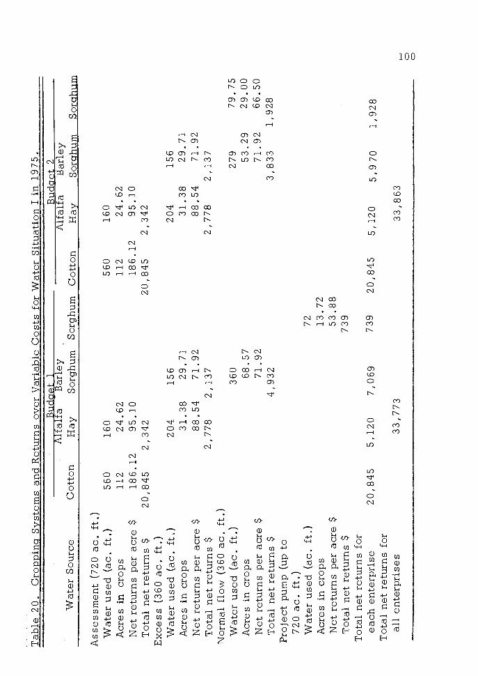
Tab
le 2
0. C
ropp
ing
Syst
ems
and
Ret
urns
ove
r V
aria
ble
Cos
ts f
or W
ater
Situ
atio
n I
in 1
975.
Wat
er S
ourc
e
Ass
essm
ent (
720
ac. f
t.)W
ater
use
d (a
c. f
t.)56
016
0A
cres
in c
rops
112
24.6
2N
et r
etur
ns p
er a
cre
$18
6.12
95.1
0T
otal
net
ret
urns
$20
,845
2,34
2E
xces
s (3
60 a
c. f
t.)
Bud
get 1
Alf
alfa
Bar
ley
Bud
oet 2
Alf
alfa
Bai
eyC
otto
nH
aySo
rghu
m S
orgh
um C
otto
nH
aySo
rqhu
mSo
rahu
rri
560
160
112
24.6
218
6.12
95.1
020
,845
2,34
2
Wat
er u
sed
(ac.
ft.)
204
156
204
156
Acr
es in
cro
ps31
.38
29.7
131
.38
29.7
1N
et r
etur
ns p
er a
cre
$88
.54
71.9
288
.54
71.9
2T
otal
net
ret
urns
$2,
778
2,13
72,
778
2,13
7N
orm
al f
low
(36
0 ac
. ft.)
Wat
er u
sed
(ac.
ft.)
360
279
79.7
5A
cres
in c
rops
68.5
753
.29
29.0
0N
et r
etur
ns p
er a
cre
$71
,92
71.9
266
.50
Tot
al n
et r
etur
ns $
4,93
23,
833
1,92
8Pr
ojec
t pum
p (u
p to
720
ac. f
t.)W
ater
use
d (a
c. f
t.)72
Acr
es in
cro
ps13
.72
Net
ret
urns
per
acr
e $
53.8
8T
otal
net
ret
urns
$73
9T
otal
net
ret
urns
for
each
ente
rpri
se20
,845
5,12
07,
069
739
20,8
455,
120
5,97
01,
928
Tot
al n
et r
etur
ns f
oral
l ent
erpr
ises
33,7
7333
,863

720
ac. f
t.)W
ater
use
d (a
c, f
t.)13
2A
cres
in c
rops
48.0
0N
et r
etur
ns p
er a
cre
$53
.88
Tot
al n
et r
etur
ns $
2 , 5
86T
otal
net
ret
urns
for
each
ent
erpr
ise
$20
,845
5,12
04,
603
2,58
620
,845
5,12
079
16,
717
Tot
al n
et r
etur
ns f
oral
l ent
erpr
ises
33,1
5433
,473
Tab
le 2
1. C
ropp
inq
Syst
ems
and
Re1
urc1
over
Var
iabl
e C
osts
for
Wat
er S
ituip
n II
in 1
975.
Wat
er S
ourc
e
Bud
get 1
Bud
get 2
Cot
ton
Alf
alfa
FI
Bar
ley
Sorg
hum
Sor
ghum
Cot
ton
Alf
alfa
Hay
Bar
ley
Sorg
huth
Sorg
hum
Ass
essm
ent (
720
ac. f
t.)W
ater
use
d (a
c. f
t.)56
016
056
016
0A
cres
in c
rops
112
24.6
211
224
.62
Net
ret
urns
per
acr
e $
186,
. 12
95.1
018
6.12
95.1
0T
otal
net
ret
urns
20,8
452,
342
20,8
452,
342
Exc
ess
(360
ac.
ft.)
Wat
er u
sed
(ac.
ft.)
204
156
204
156
Acr
es in
cro
ps31
.38
29.7
131
.38
56.7
2N
et r
etur
ns p
er a
cre
$88
.54
71.9
288
.54
66.5
0T
otal
net
ret
urns
$2,
778
2,13
72,
778
3,77
2N
orm
al f
low
(18
0 ac
, ft.)
Wat
er u
sed
(ac.
ft.)
180
57.7
512
1.77
Acr
es in
cro
ps34
.29
11.0
044
.28
Net
ret
urns
per
acr
e $
71.9
271
.92
66.5
0T
otal
net
ret
urns
$2,
466
791
2,94
5Pr
ojec
t pum
p (u
p to

Tab
le 2
2.C
ropp
ing
Syst
ems
and
Ret
urns
ove
r V
aria
ble
Cos
ts f
or W
ater
Situ
atio
n II
I in
197
5,.
Bud
get 1
Bud
get 2
Wat
er S
ourc
eC
otto
nA
lfal
faH
ayB
arle
ySo
rghu
m S
orgh
um C
otto
nA
lfal
faH
ayB
arle
ySo
rghu
mSo
rghu
m
Ass
essm
ent (
720
ac. f
t.)W
ater
use
d (a
c. f
t.)56
016
056
016
0A
cres
in c
rops
112
24.6
211
224
.62
Net
ret
urns
per
acr
e $
186.
1295
.10
186.
1295
,10
Tot
al n
et r
etur
ns $
20,8
452,
342
20,8
452,
342
Exc
ess
(30
acre
ft.)
Wat
er u
sed
(ac.
ft.)
204
156
204
156
Acr
es in
cro
ps31
.38
29.7
131
.38
56.7
2N
et r
etur
ns p
er a
cre
$88
.54
71.9
288
.54
66.5
0T
otal
net
ret
urns
$2,
778
2,13
72,
778
3,77
2Pr
ojec
t pum
p (u
p to
720
ac. f
t.)W
ater
use
d (a
c. f
t.)22
6.30
152
Acr
es in
cro
ps82
.29
55.2
8N
et r
etur
ns p
er a
cre
$53
.88
53.8
8T
otal
net
ret
urns
$4,
434
2,97
9T
otal
net
ret
urns
for
each
ent
erpr
ise
$20
,845
5,12
02,
137
4,43
420
,845
5,12
0.6,
751
Tot
al n
et r
etur
ns f
oral
l ent
erpr
ises
$32
,536
32,7
16

Tab
le 2
3C
ro..i
n. S
ste
ms
and
Ret
urns
ove
r V
aria
ble
Cos
ts f
or W
ater
Situ
atio
n IV
in 1
975.
Bud
get 1
Bud
get 2
Wat
er S
ourc
eC
otto
nA
lfal
faH
ayB
arle
ySo
rghu
m S
orgh
um C
otto
nA
lfal
faH
ayB
arle
ySo
rghu
mSo
rghu
m
Ass
essm
ent (
720
ac. f
t.)W
ater
use
d (a
c. f
t.)56
016
056
016
0A
cres
in c
rops
112
24.6
211
224
.62
Net
ret
urns
per
acr
e $
186
1295
.10
186.
1295
.10
Tot
al n
et r
etur
ns $
20,8
452,
342
20,8
452,
342
Exc
ess
(360
ac.
ft.)
Wat
er u
sed
(ac.
ft.)
204
156
204
156
Acr
esin
crop
s31
.38
29.7
131
.38
56.7
2N
et r
etur
ns p
er a
cre
$88
.54
71.9
288
.54
66.5
0T
otal
net
ret
urns
$2,
778
2,13
72,
778
3.77
2Pr
ivat
e pu
mp
(up
to72
0 ac
. ft.)
Wat
er u
sed
(ac.
ft.)
226.
3015
2A
cres
in c
rops
82.2
955
.28
Net
ret
urns
per
acr
e $
49.6
749
.67
Tot
al n
et r
etur
ns $
4,08
72,
746
Tot
al n
et r
etur
ns f
orea
ch e
nter
pris
e $
20,8
455,
120
2,13
74,
087
20,8
455,
120
6,51
8T
otal
net
ret
urns
for
all e
nter
pris
es $
32, 1
8932
,483

104
In budget 2 the acreage of cotton and of alfalfa hay irrigated with
the lowest cost water were the same as in budget 1. The remaining acreages
and crops were organized so that 29. 71 acres of barley-sorghum were irri-
gated with excess water, and 53.29 acres of barley-sorghum and 29 acres
of sorghum were irrigated with normal flow water. Note that in this setting
of crops and their respective acreages, all surface water was utilized and
all the cropland acreage was irrigated. The cropping system developed
under this budget was 112 acres of cotton, 56 acres of alfalfa hay, 83
acres of barley-sorghum and 29 acres of sorghum.
Comparing the two budgets, note that while the returns from
cotton, alfalfa and barley-sorghum with assessment and excess water
were the same in the two budgets, the returns from barley-sorghum and sor-
ghum with normal flow water were $829 higher in budget 2 than returns from
barley-sorghum with the same water source in budget 1, but while in
budget 2 all the cropland acres were irrigated with surface water, in
budget 1, 13. 72 acres were put under the highest profitable crop with
pump water--sorghum, with the result that returns over variable costs
were $90 less than in budget 2. Therefore, the cropping system of budget
2 catered to optimum farm organization for water situation I. Moreover,
it is to be noted that the cropping system in budget 2 utilized a smaller
amount of water than that of budget 1.

105
Budgets for water situation II
With water situation II note that in budget 1 the acreages of
cotton, alfalfa hay and barley-sorghum irrigated with assessment and
excess water were the same as in budget 1 of water situation I; water
from normal flow and project pump were used for 34.29 acres of barley-
sorghum and 48 acres of sorghum respectively. The cropping system de-
veloped by this procedure is 112 acres of cotton, 56 acres of alfalfa hay,
66 acres of barley-sorghum and 48 acres of sorghum.
In budget 2 the acreages of cotton, and of alfalfa hay were irri-
gated with the lowest cost water, the same as in budget 1. The remaining
excess water was used for 56.72 acres of sorghum, and the normal flow
water was used for 44.28 acres of sorghum and 11 acres of barley-sor-
ghum. Note that in this budget all surface water was utilized, and all
the cropped land was irrigated, and no project pump water was used.
The cropping system in budget 2 was 112 acres cotton, 56 acres alfalfa
hay, 11 acres barley-sorghum and 101 acres of sorghum.
While returns from cotton and alfalfa hay were the same in
budgets 1 and 2, returns from sorghum with excess water in budget 2
were $1,635 higher than returns in budget 1 from barley-sorghum with
the same amount of excess water. With the normal flow water the re-
turns from sorghum and barley-sorghum were $1,270 higher than returns
from barley-sorghum in budget 1, The total increase in returns from crops
with surfaoe water in budget 2 over that in budget 1 was $2,905. But

106
note that while in budget 2 all the cropped land was irrigated with the
surface water, only 64 acres were irrigated in budget 1 with a reduction
of 48 acres. However, when these 48 acres were put under the highest
profitable crop with project pump water--sorghum, they yielded a return
of $2,586 which is $319 less than the increase obtained by allocating
the surface water such that all the cropped land was irrigated. The
cropping system system developed under budget 2,, therefore is more
profitable than for budget 1 in water situation II,
Budgets for water situation III
With water situation III note that in budget 1 cotton, alfalfa hay
and barley-sorghum irrigated with assessment and excess water are the
same as in budget 1 of the previous water situations. With project pump
water sorghum is the highest profitable crop after cotton and alfalfa and
82.29 acres were included. The cropping system developed under budget
1 was 112 acres of cotton, 56 acres of alfalfa hay, 29.71 acres of barley-
sorghum and 82.29 acres of sorghum.
In budget 2 of water situation III the acreages of cotton and al-
falfa hay were irrigated with the lowest cost water (Table 22). The balance
of the excess water was used to irrigate 56.72 acres of sorghum. The re-
maining 55.28 unirrigated acres were used for sorghum and were irri-
gated with project pump water. The cropping system for budget 2 was
112 acres of cotton, 56 acres of alfalfa hay and 112 acres of sorghum.
107
On comparing the two above budgets note that while in budget 1
some barley-sorghum was grown, in budget 2 all the grain acreage was
put under sorghum. The returns over variable costs from cotton and al-
faif a hay were the same in both budgets, but the returns from sorghum
with excess water in budget 2, were $1, 635 higher than the returns from
barley-sorghum in budget 1 irrigated with the same amount of excess
water. Growing only 29.71 acres of barley-sorghum with excess water
would leave 27 acres (56. 72-29. 71) unirrigated relative to the acres irri-
gated with excess water in budget 2. However, when these 27 acres were
planted with sorghum and irrigated with project pump water they yield a
return $180 less than the increase in return obtained in budget 2 as dis-
cussed above. Therefore, the cropping system developed for budget 2 is
more profitable than that for budget 1 with water situation III.
Budgets for water situation IV
The reader may realize that water situation III and IV have many
things in common. Both water situations have equal rights to surface
water, have no rights to normal flow water and both depend on groundwater
to supplement surface water. The only difference between them is that
water situation III has access to project pump water through its project
pump right while water situation IV has a private well and pump. Since
the relative profitability in both water situations with each water source
is the same, then the same budgets developed for water situation III and

108
the related discussion will be applicable to water situation IV as is evi-
dent from Tables 22 and 23. For this reason no further discussion of water
situation IV is given here.
Comparison of Cropping Systems in 1965 and 1975
On comparing the cropping systems developed for periods 1965
and 1975 it is to be noted that while the optimum cropping system for each
water situation in 1965 was the same, the cropping systems in 1975 were
different in water situation I, II, and III and IV. This means that while
the water rights had no effect on the cropping system in 1965 they did
affect farm organization in 1975. This was caused by a change in the
relative profitability of sorghum in 1975. With the yields, prices and
costs used in the budgets sorghum was more profitable relative to other
crops in 1975 than in 1965. This was due to increase in returns over
variable costs brought about primarily by increase in yields in 1975 (see
Table 14). This change also caused sorghum returns per acre foot of water
to increase relative to other crops. Thus, in the 1975 period greater re-
turns over variable costs were realized from sorghum with surface water
than by using the limited surface water to produce barley-sorghum and
producing sorghum on the remaining acreage with groundwater.
It is to be noted that the farm organizations in 1975 utilized
less groundwater than the farm organization in 1965 since it grew more
sorghum than barley-sorghum. Under these circumstances the farmer in

109
1975 would not need to worry so much about the continuous declining
water table and increasing groundwater costs since they would not depend
on groundwater to the extent that they do in 1965.
Returns to and Indicated Value of Land in 1965 and 1975
From the returns over variable costs obtained in the above budgets
(Table 18 through 23), cash and non-cash overhead costs other than returns
to land were deducted. The residual thus obtained constitutes the returns
to land (Table 24). Cash and non-cash overhead costs used above were
taken from Table 15 of the text.
Once returns to land have been estimated, an indicated value may
be computed for the land by capitalization. Capitalization is the process12
by which value is derived from annual returns. It requires two factors:
an estimate of annual net returns and a capitalization rate 13 The annual
returns to land estimated above for each water situation in the two periods
were divided by 360, the total acres of the farm, in order to get the annual
returns to land per acre. The capitalization rate expresses the relation-
ship between an annual return and the value of the property. A capitali-
zation rate of 5 percent was used in this study and was chosen as a repre-
sentative of the opportunity return which might be realized from the capital
Net returns here means returns over and above all costs otherthan returns to real estate.
William G. Murray, Farm Appraisal and Valuation, Iowa State,Ames, 1961, p. 238.

110
invested in land. Therefore the indicated value is an indicated 'oppor-
tunity value' of the land.
The capitalization rate however may vary from one water situation
to the other depending among other factors on the degree of risk involved
in each case. The reader may recognize that water situation II does not
get a constant one-half acre foot of normal flow water year after year but
that this amount represents an average over a period of time, whereas with
water situation I the normal flow is somewhat more dependable. Therefore,
the risk involved in the two situations is not the same and hence the capi-
talization rate in water situation II perhaps should be somewhat higher
than in situation I due to the greater risk involved.
Assuming that the project will be able to continue supplying
assessment, excess and groundwater at the present level and that the
farmer with a private well and pump is concerned about a declining water
table and all related items, then the risk involved in water situation IV is
greater than the risk involved in water situation III, ceteris paribus,
and therefore the capitalization rate of water situation IV perhaps should
be higher than that of water situation III. But because of the lack of in-
formt1on as to the relative magnitude of the risks involved only one capi-
talization rate was used in this study, with the recognition that the indi-
cated value estimated may vary.
On comparing the indicated value of land in each water situation,
note that these values vary from one water situation to the other and from

Tab
le 2
4. R
etur
ns O
ver
Var
iabl
e C
osts
, Cas
h an
d N
on-c
ash
Ove
rhea
d C
osts
,R
etur
ns to
Lan
d an
d th
eIn
dica
ted
Val
ue o
f L
and
with
the
Four
Wat
er S
ituat
ions
the
Salt
Riv
er P
ro e
ct19
65 a
nd 1
975
a.O
ther
than
ret
urns
to la
nd.
Item
Wat
er S
ituat
ion
IW
ater
Situ
atio
n II
Wat
er S
ituat
ion
III
Wat
er S
ituat
ion
IV19
6519
7519
6519
7519
6519
7519
6519
75
Dol
lars
Ret
urns
ove
r va
riab
leco
sts
31,7
5833
,863
30,9
3233
,473
30,1
0532
,716
30,3
2632
,483
Ove
rhea
d ca
sh c
osts
3,29
93,
940
3,29
93,
940
3,29
93,
940
3,55
24,
227
Bal
ance
28,4
5929
,923
27,6
3329
,533
26,8
0628
,776
26,7
7428
,256
Ove
rhea
d no
n-ca
shco
stsa
13,9
2314
,431
13,9
2314
,431
13,9
2314
,431
15,1
9015
,967
Ret
urns
to r
eal e
s-ta
te14
,536
15,4
9213
,710
15,1
0212
,883
14,3
4511
,584
12,2
89
Ret
urns
to la
nd p
erac
re40
4338
4236
4032
34
Indi
cate
d va
lue
ofla
nd p
er a
cre
capi
-ta
lized
at 5
%80
086
076
084
072
080
064
068
0

112
period to period. The variation within a period was because the returns to
land obtained in each water situation were different. Note with reference to
Table 24 that the overhead costs were the same in water situations I, II and
III and higher in water situation TV by the amount of overhead costs of the
private well, pump and motor (see Table 15), Since the returns over variable
costs for the first three water situations varied and since these situations
have the same overhead costs, then the returns to land were highest for
situation I, followed in order by II and then III. However when water situ
ation IV is compared with the former three, the higher level of overhead costs
results in ranking it last with respect to returns to land. The relative indi-
cated value of land therefore is highest for water situation I followed by
water situation II then III and last IV. However it is to be recognized that
although water situation IV has a comparatively low indicated value to land,
the presence of a private well and pump in the above situation may make
the actual value higher than the estimated indicated value. The capital
investment in the well and pump which was deducted in the form of de-
preciation in arriving at returns to land, may be paid by the purchaser of
the real estate over and above the indicated value derived by capitalization.
It is to be noted however the above indicated value of land is not
absolute and may vary more or less with any individual farm. The esti-
mated value given above does not include income associated with houses,
location and other intangible features.

113
From the above discussion note that while the water rights had no
effect on the cropping system in 1965 their effect on land value resulted in
different indicated values of land in the four water situations. With res-
pect to 1975 it is to be noted that water rights affected both cropping
systems and land values.
The indicated value of land in the two periods showed an in-
crease in the indicated value of land in 1975 relative to 1965.

CHAPTER IV
SUMMARY AND CONCLUSIONS
This study pertains to the Salt River Project in central Arizona,
a non-profit organization which provides irrigation water for farms within
its boundaries.
Water is the primary limiting factor in agricultural production in
this area. Crop production is dependent upon irrigation since precipi-
tation averages only about eight inches annually.
The objective of this study is twofold: to examine the organi-
zation and operation of the Salt River Project and to analyze the effect of
water rights on farm organization and value. Only limited work has been
done heretofore in these areas. Treatment of the first objective is pri-
marily descriptive, based largely upon first-hand knowledge gained in
personal study and observation of the Project, In analysis of the second
objective budgets were constructed as of 1965 and 1975 for a medium
sized 360 acre farm, assuming various representative water situations
to show the effect of water rights upon the cropping system and upon
indicated land values assuming the goal of management to be maximi-
zation of income. Data for the budget analysis were primarily from
A. G. Nelson, major porfessor, Department of Agricultural Economics,
and judgment of other departments in the College of Agriculture,
114

115
University of Arizona, supplemented by information from the United States
Department of Agriculture.
The budgets were based upon estimated yields, prices and costs
expected to be realized during 1965 and 1975. The yields, prices and
costs used in the budgets were estimated at approximately the level pre-
vailing in the area in the 1965 period. In the 1975 period, yields and
fertilizer application were increased to account for anticipated increased
adoption of presently known tebhnology. Cotton lint prices were antici-
pated to fall while cotton seed prices to rise, and wages, management
and real estate taxes were expected to increase relative to 1965.
The Salt River Project is comprised of the Salt River Valley Water
Users' Association and the Salt River Project Agricultural Improvement
and Power District. While the Association and Power District are separate
legal entities each with its own board of directors, the two boards have
always been one and the same, elected by the shareholders in the Project.
The Project is administered by a general manager who is responsible for
both the irrigation and power phases. Two associate general managers
and three assistant general managers assist in carrying out functions of
the Power District, while one associate general manager assists on the
Water Users' Association side.
The Project obtains its water from a series of dams on the rivers
in the watershed located east and north of the Project and from wells
located within the Project. To carry out functions involved in supplying

116
water to its users, the Salt River Project Water Users Association is
divided into five departments: watershed, irrigation operation, irrigation
service, engineering and construction and maintenance. The watershed
department observes, records and takes necessary action for the pro-
tection of water supply from uses by others not entitled to it, and for
conserving this water supply for the project storage system, and provides
annual forecasts of the expected water yield. The irrigation operation
department delivers with a minimum of loss the stored and developed
water to the land within the Project on demand of the shareholders. The
irrigation service department properly administers the water rights of all
land within the boundary of the Project. The engineering department pro-
vides the engineering and technical skills in construction, maintenance
and research for the irrigation transmission, distribution and groundwater
system, to maintain proper efficiency of water delivery to the shareholders
of the Project. The construction and maintenance department maintains
the irrigation facilities in a condition that will permit economical and
efficient operation of the system.
Electric power distributed by the Project is obtained from hydro-
electric plants on four of the six storage dams in the watershed and six
thermal-electric plants within the Project, The power phase of the Project's
operation provides a substantial subsidy for irrigation and domestic water.
The water made available by the Salt River Project to its share-
holders is allotted among the farms according to water rights as established

117
in 1910 by the Kent decree. Water rights are now of three types: Class
A rights, Class B and C, and pump rights. Class A rights include the
normal flow rights which represent rights to that water carried by rivers
and which is not restricted by impounding. These rights cover an area
148, 753 acres comprising the land which was under continuous irrigation
year after year from 1869 to 1909. The 1869 land has first priority in
rights followed in order by 1870 and so on to 1909. Normal flow rights
should be used within the following eight days, otherwise they are lost.
Land with Class A rights also has equal rights to stored and developed
water along with other land in the Project. Class B and C rights pertain
to the water stored and developed over and above that taken by farmers
having Class A rights. They include assessment and excess water the
benefits of which are equally distributed among all acres in the Project.
The pump rights represent rights to pumped water made available
by the Project to those farmers who purchased a pump right at the time
they were offered for sale. All water rights adhere to the land; they cannot
be bought or sold. In addition, many of the farms in the Project have
private wells.
Within this framework, water rights of farms in the Project may
be classified into four groups referred to in this study as water situations'

118
according to the source of the water the farms receive. These are as
follows:
Water Situation I Water Situation II Water Situation III Water Situation IV
Assessment Assessment Assessment AssessmentExcess Excess Excess ExcessNormal Flow Normal Flow - -(early right) (late right)Project Pump Project Pump Project Pump
- - - Private Pump
Four major field crops typical of the area were included in the
budgets: cotton, alfalfa hay, barley and sorghum, Barley-sorghum
double-cropped was also included, making a total of five enterprises,
Returns over variable costs per acre were calculated for each crop. The
ranking of the crop enterprises in terms of returns over variable costs for
each of the four water situation in 1965 and 1975 is as follows:
Water Sources 1975
Note that while the relative profitability of crops was the same in all
water sources in 1965, in 1975 the relative profitability of these crops
with surface water sources was different from the groundwater source.
In preparing budgets for the farm, the first approach was to
allocate acreage to the most profitable crop up to the limit of governmental
Rank All Water Sources 1965Assessment, Excessand Normal Flow
Project Pump andPrivate Pump
1 Cotton Cotton Cotton2 Alfalfa Hay Alfalfa Hay Alfalfa Hay3 Barley Sorghum Barley Sorghum Sorghum4 Sorghum Sorghum Barley Sorghum5 Sorghum after Barley Sorghum after Barley Sorghum after Barley6 Barley Barley Barley

119
acreage allotment or rotational restrictions, then to the crop which ranked
second in profitability and so on until the entire cropland acreage was
utilized. This budget procedure gave the highest farm returns over variable
costs for the 1965 period. However, in the 1975 period, higher farm
returns over variable costs were obtained when the entire cropland
acreage in the farm was utilized, but more of the acreage was used for
sorghum as a single crop. This was due to the change in the relative
profitability of sorghum in 1975. With the yields, prices and costs used
in the budgets, sorghum was more profitable relative to other crops in
197 than in 1965. This change also caused sorghum returns per acre
foot of water to increase relative to other crops. Thus, in the 1975 period,
greater returns over variable costs were realized from sorghum with
surface water than by using the limited surface water to produce
barley-sorghum and producing sorghum on the remaining acreage with
groundwater.

120
The cropping systems which gave the highest returns over variable
costs are as follows:
1965, All 1975 Water SituationsCrop Water Situations I II Ill
(Acres) (Acres)
Overhead cash and non-cash costs other than returns to land were
deducted from returns over variable costs to obtain returns to land for each
of the water situations in 1965 and 1975. Returns to land were then capi-
talized to obtain an indicated value of land with each of the water situ-
ations in the two periods. A capitalization rate of 5 percent was used,
estimated to be the rate which might be earned on capital invested in the
farm if it were placed in non-farm investments. Thus, no recognition was
given to location, home value and the like in the estimated values. The
analysis indicates, however, that water rights have an effect on the capi-
talized value of land in the Project.
Comparison of the indicated values shows that these values vary
from one water situation to another in the two periods and from period to
period. They were highest for water situation I followed in order by water
situation II, then water situation III and last IV.
The conclusion indicated by this study is that under current con-
ditions water rights probably have no effect on the cropping system but
probably do affect land values. Looking to the future, water rights may
Cotton 112 112 112 112 112Alfalfa Hay 56 56 56 56 56Barley Sorghum 112 83 11 - -Sorghum - 29 101 112 112

121
affect both cropping systems and the value of land. Moreover, with the
levels of prices, yields and costs used in 1965 and 1975 the analysis
indicates capitalized values of land would increase over the coming
decade.

LITERATURE CITED
Barr, George W., ed. Recovering Rainfall. University of Arizona,Tucson, 1956.
Glenn, Brandow W. Historical Documents Pertaining to Power Contractsand Areements of The Salt River Project. Salt River Project,Phoenix, Arizona, 1961.
Heady, Earl 0. Economics of Agricultural Production and Resource Use.Prentice-Hall Inc., Englewood Cliffs, New Jersey, 1961.
Kent, Edward, Chief Justice. Original No. 4564 Decree March 10, 1910.Third Judicial District, Phoenix, Arizona, 1910.
Kleinman, Alan P. "The Cost of Pumping Irrigation Water in CentralArizona." Unpublished Master's thesis, University of Arizona,Tucson, 1964.
Leftwich, Richard H. The Price System And Resource Allocation. Holt,Rinehart and Winston, New York, 1960,
Menzie, Elmer L. "Arizona Farm Income Leads Nation." ProgressiveAgriculture in Arizona. Vol. XVI, No. 2, University of Arizona,Tucson, March-April, 1964.
Nelson, Aaron G. "Costs And Returns For Major Field Crops In CentralArizona By Size Of Farm." Arizona Agricultural Experimental StationTechnical Bulletin in preparation, University of Arizona, Tucson.
Salt River Project. Major Facts In Brief. Phoenix, Arizona, 1961.
Articles of Incorporation of Salt River Valley Water Users'Association. Phoenix, Arizona.
Annual Reports. 1959 through 1963.
Crop Reports. 1957 through 1962, Phoenix, Arizona.
Shadegg, Stephen C. The Phoenix Story, An Adventure In Reclamation.Phoenix, Arizona, 1958.
122

123
U. S. Department of Agriculture. Aqricultural Price and Cost ProjectionsFor Use in Making Benefit and Cost Analyses of Land and WaterResource Projects. Washington, D. C., September, 1957.
Agricultural Statistics. U. S. Government Printing Office,Washington, D. C., 1963.
Farm Real Estate Taxes, Recent Trends and Developments.ARS. 43-130, August8 1960.
U. S. Department of Commerce, Bureau of the Census. U. S. Census ofAgriculture, Arizona Counties. 1959.
White, Natalie D., R. S. Stulik and others. Annual Report on GroundWater In Arizona, Spring 1962 to Spring 1963. U. S. GeologicalSurvey, Bulletin No. 15, Phoenix, Arizona8 1963.