fasst manual - montefiore institute ulgphillips/fasst_manual.pdf · 2013-02-25 · fasst manual...
TRANSCRIPT

FASST manual
FASST developpers at the Cyclotron Research Centre
Jessica SchrouffDorothee Coppieters
Remy LehembreYves LeclercqPierre Maquet
Quentin NoirhommeChristian DegueldreChristophe Phillips
Cyclotron Research CentreUniversity of Liege, B30
8 Allee du Six Aout4000 Liege, BELGIUM
http://www.montefiore.ulg.ac.be/~phillips/FASST.html
February 19, 2013

CONTENTS 2
Contents
1 Introduction 3
2 Installing & launching the toolbox 4
2.1 Installation . . . . . . . . . . . . . . . . . . . . . . . . . . . . . . . . . . . . . . . . 5
2.2 Launching and batching . . . . . . . . . . . . . . . . . . . . . . . . . . . . . . . . . 5
3 Data format & channels setup 5
3.1 Data format conversion with FASST . . . . . . . . . . . . . . . . . . . . . . . . . . 7
3.1.1 Brain Products data format conversion . . . . . . . . . . . . . . . . . . . . . 7
3.1.2 Other data format conversion . . . . . . . . . . . . . . . . . . . . . . . . . . 7
3.2 Channel definition . . . . . . . . . . . . . . . . . . . . . . . . . . . . . . . . . . . . 8
4 Main functions of the toolbox 8
4.1 General tools . . . . . . . . . . . . . . . . . . . . . . . . . . . . . . . . . . . . . . . 9
4.1.1 Displaying one M/EEG data file . . . . . . . . . . . . . . . . . . . . . . . . 9
4.1.2 Comparing multiples M/EEG data files . . . . . . . . . . . . . . . . . . . . 12
4.1.3 Appending M/EEG data files . . . . . . . . . . . . . . . . . . . . . . . . . . 13
4.1.4 Chunking a time window from an M/EEG data file . . . . . . . . . . . . . . 14
4.1.5 Computing the spectrogram of one M/EEG data file . . . . . . . . . . . . . 14
4.1.6 Displaying the spectrogram or power spectrum of an M/EEG data file . . . 15
4.2 EEG-MRI artefact rejection tools . . . . . . . . . . . . . . . . . . . . . . . . . . . . 16
4.2.1 Gradient artefact rejection . . . . . . . . . . . . . . . . . . . . . . . . . . . . 16
4.2.2 Pulse artefact rejection . . . . . . . . . . . . . . . . . . . . . . . . . . . . . 18
4.3 Sleep specific tools . . . . . . . . . . . . . . . . . . . . . . . . . . . . . . . . . . . . 20
4.3.1 Manual sleep scoring . . . . . . . . . . . . . . . . . . . . . . . . . . . . . . . 20
4.3.2 Spectral power calculation and statistics . . . . . . . . . . . . . . . . . . . . 22
4.4 Automatic wave detection tools . . . . . . . . . . . . . . . . . . . . . . . . . . . . . 22
4.4.1 Slow Wave detection . . . . . . . . . . . . . . . . . . . . . . . . . . . . . . . 23
4.4.2 Sleep Spindles detection (BETA version!) . . . . . . . . . . . . . . . . . . 26
CONTENTS 3
5 Advanced Users 30
5.1 Addition to the SPM8 structure . . . . . . . . . . . . . . . . . . . . . . . . . . . . . 30
5.1.1 The D.info field . . . . . . . . . . . . . . . . . . . . . . . . . . . . . . . . . 30
5.1.2 The D.CRC field . . . . . . . . . . . . . . . . . . . . . . . . . . . . . . . . . . 30
5.2 “Hidden” functions . . . . . . . . . . . . . . . . . . . . . . . . . . . . . . . . . . . . 32
6 Acknowledgments 32

1 INTRODUCTION 4
1 Introduction
“FASST” stands for “fMRI Artefact rejection and Sleep Scoring Toolbox”. This M/EEG toolboxis developed by researchers from the Cyclotron Research Centre, University of Liege, Belgium,with the financial support of the Fonds de la Recherche Scientifique-FNRS, the Queen Elizabeth’sfunding, and the University of Liege. On Dr. Pierre Maquet’s impulse we started writing thesetools to analyze our sleep EEG-fMRI data and tackle four crucial issues:
Continuous M/EEG. Long multi-channel recording of M/EEG data can be enormous. Thesedata are cumbersome to handle as it usually involves displaying, exploring, comparing,chunking, appending data sets, etc.
EEG-fMRI. When recording EEG and fMRI data simultaneously, the EEG signal acquiredcontains, on top of the usual neural and ocular activity, artefacts induced by the gradientswitching and high static field of an MR scanner. The rejection of theses artafacts is noteasy especially when dealing with brain spontaneous activity.
Scoring M/EEG. Reviewing and scoring continuous M/EEG recodings, such as is commonwith sleep recordings, is a tedious task as the scorer has to manually browse through theentire data set and give a “score” to each time-window displayed.
Waves detection. Continuous and triggerless recordings of M/EEG data show specific wavepatterns, characteristic of the subject’s state (e.g., sleep spindles or slow waves). Theirauomatic detection is thus important to assess those states.
Currently the toolbox can efficiently deal with these issues, as described in section 4. Eventhoughthe toolbox was originally divised for EEG data, it also handles MEG and LFP data without anyproblem, if in the right format (see section 3). FASST is in effect an add-on toolbox for SPM8[?, ?]and relies on SPM8 data format and functions to perform some operations.
Troubles usually come from the data format and channel setup but see section 3 for FASSTrequirements and solutions. The “eye-balling” and manipulation of continuous multi-channelrecordings is eased by a series of tools (see section 4.1). Specifically, for EEG-fMRI acquisi-tions (see section 4.2), FASST can operate directly on the raw data acquired with a “BrainAmpMR” system (Brain Products GmbH, Gilching, Germany) and includes the well-known AASmethod[?] for the “gradient artefact” rejection, as well as the recently published “constrainedICA” method[?] for the rejection of the “pulse artefact”. Other “classic” methods for the “pulseartefact” rejection are also available. And an easy GUI is available for the manual scoring of sleepEEG by different users (see section 4.3). Some statistics and sleep specific features can then beautomatically extracted.
FASST is available for free, under the GNU-GPL and, obviously, it comes without any war-ranty: you should use it at your own risk. This is an ongoing research project and we plan toadd new features and functionalities, according to our own needs and the feedback from users. Ifyou are happy with the results obtained with FASST and publish them, please use the followingreferences:
• for the toolbox in general and the sleep specific tools[?, ?]
J. Schrouff, D. Coppieters, R. Lehembre, Y. Leclercq, P. Maquet,
Q. Noirhomme, C. Degueldre, E. Balteau, and C. Phillips,
fMRI Artefact rejection and Sleep Scoring Toolbox (FASST).
Cyclotron Research Centre, University of Liege, Belgium, 2009.
http://www.montefiore.ulg.ac.be/~phillips/FASST.html

2 INSTALLING & LAUNCHING THE TOOLBOX 5
and
Y. Leclercq, J. Schrouff, Q. Noirhomme, P. Maquet, C. Phillips,
‘‘fMRI Artefact rejection and Sleep Scoring Toolbox’’,
Computational Intelligence and Neuroscience, 2011.
http://www.hindawi.com/journals/cin/2011/598206/
• for the constrained ICA “Pulse artefact” rejection method[?] in particular
Y. Leclercq, E. Balteau, T. Dang-Vu, M. Schabus, A. Luxen, P. Maquet, and
C. Phillips.
‘‘Rejection of pulse related artefact (PRA) from continuous electroencepha-
lographic (EEG) time series recorded during functional magnetic resonance
imaging (fMRI) using constraint independent component analysis (cICA)’’,
NeuroImage, 44(3):679-691, 2009.
Note that FASST includes a few routines from 3 other freely available toolboxes:
• EEGLAB[?, ?], mainly for a few functions used by the constrained ICA “pulse artefact”rejection, available from http://sccn.ucsd.edu/eeglab/;
• the FMRIB plug-in for EEGLAB[?], for the ECG peak detection and classic PCA/Gaussianmean “pulse artefact” rejection, available from http://users.fmrib.ox.ac.uk/~rami/
fmribplugin/;
• the “Mutual Information computation” package[?], for some the selection of correctionmatrices during cICA “pulse artefact” rejection, available from http://penglab.janelia.
org/proj/mRMR/.
We thank their authors for letting us use their work.
We would also be thankful to hear from you if you find bugs in the code. Feel also free tosubmit add-ons to this toolbox but please note that support will not be provided for “home-made”changes of the distributed code.
2 Installing & launching the toolbox
In order to work properly, FASST needs to have those 2 softwares installed:
• a recent version of Matlab , we used version 7.5 (R2007b) to develop FASST. Any laterMatlab version should work, in theory.
• the latest version of the “Statistical Parametric Mapping Software”, i.e. SPM8 [?, ?].You can download it from: http://www.fil.ion.ucl.ac.uk/spm/software/. Install itin a suitable directory, for example C:\SPM8\, and make sure that this directory is on theMatlab path1.
NOTE: Originally FASST relied on routines from Matlab “Signal Processing Toolbox” forsome filtering functions. In this version we have tried to lift this requirement. If you do not havethe toolbox, filtering and time-frequency operations are executed by freely available equivalents2
distributed under the GNU General Public License .1No need to include the subdirectories!2see in the subdirectory \FASST\SPTfunctions.

3 DATA FORMAT & CHANNELS SETUP 6
2.1 Installation
After registering and downloading the zipped file containing FASST, the installation proceeds asfollow:
1. Uncompress the zipped file in your favourite directory, for example C:\FASST\;
2. Launch Matlab ;
3. Go to the “File” menu → “Set path”;
4. Click on the “Add folder” button and select the FASST folder, i.e. C:\FASST\ if you fol-lowed the example;
5. Click on save.
A few routines from the “Mutual Information computation” package[?] are written in C++(.cpp files) and should thus be compiled for your specific operating system. We are providingthese compiled routines for the usual OS’s such as: Windows XP (32 bits), Windows 7 (64 bits),Mac OS 10, Linux (32 bits). If your OS is not listed (or routines do not work properly), you cancompile the routines with the makeosmex.m script available in the MInfo subdirectory.
2.2 Launching and batching
Once installed, there are three ways to call up FASST functionalities:
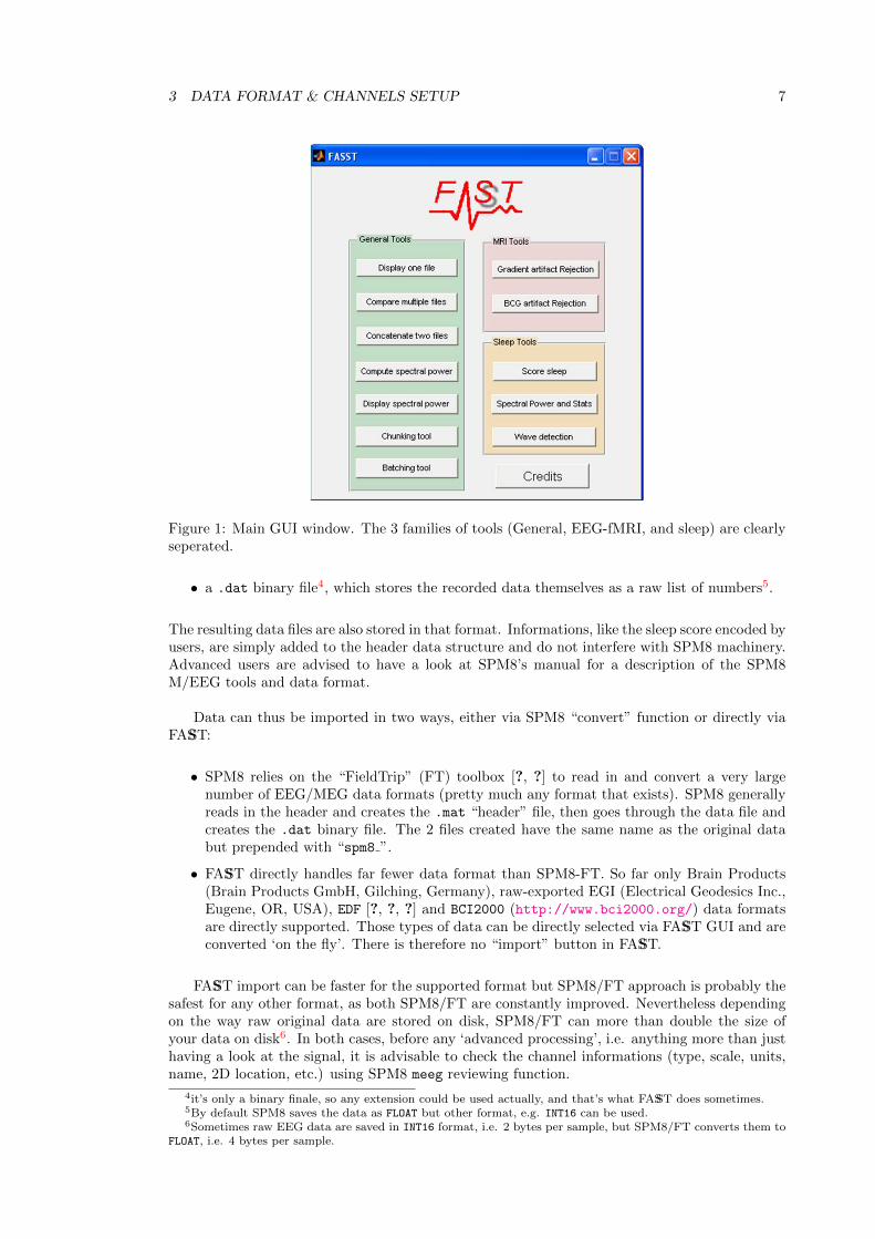
• to launch the toolbox GUI, just type crc main or fasst at the Matlab prompt and themain GUI figure will pop up, see Fig. 1. From there on simply click on the tool you wantto use;
• some functions of FASST have been integrated into SPM8 matlabbatch batching system [?],the batching GUI is launched by typing crc batch at the Matlab prompt3;
• most tools can also be called individually by calling them directly from the Matlab prompt,or for scripting in a .m file.
3 Data format & channels setup
Data format is always an issue in EEG and MEG since each company enjoys his own specific(and usually proprietary) format. So we decided to use the Matlab based and open SPM8 meeg
data format. Therefore FASST internally works with SPM8 meeg data format:
• a .mat “header” file, which contains all the information about the data (channel names andtypes, sampling rate, stimuli, data format, etc.) as well as room for user-specific data; and
3check SPM8’s manual for more information about matlabbatch
3 DATA FORMAT & CHANNELS SETUP 7
Figure 1: Main GUI window. The 3 families of tools (General, EEG-fMRI, and sleep) are clearlyseperated.
• a .dat binary file4, which stores the recorded data themselves as a raw list of numbers5.
The resulting data files are also stored in that format. Informations, like the sleep score encoded byusers, are simply added to the header data structure and do not interfere with SPM8 machinery.Advanced users are advised to have a look at SPM8’s manual for a description of the SPM8M/EEG tools and data format.
Data can thus be imported in two ways, either via SPM8 “convert” function or directly viaFASST:
• SPM8 relies on the “FieldTrip” (FT) toolbox [?, ?] to read in and convert a very largenumber of EEG/MEG data formats (pretty much any format that exists). SPM8 generallyreads in the header and creates the .mat “header” file, then goes through the data file andcreates the .dat binary file. The 2 files created have the same name as the original databut prepended with “spm8 ”.
• FASST directly handles far fewer data format than SPM8-FT. So far only Brain Products(Brain Products GmbH, Gilching, Germany), raw-exported EGI (Electrical Geodesics Inc.,Eugene, OR, USA), EDF [?, ?, ?] and BCI2000 (http://www.bci2000.org/) data formatsare directly supported. Those types of data can be directly selected via FASST GUI and areconverted ‘on the fly’. There is therefore no “import” button in FASST.
FASST import can be faster for the supported format but SPM8/FT approach is probably thesafest for any other format, as both SPM8/FT are constantly improved. Nevertheless dependingon the way raw original data are stored on disk, SPM8/FT can more than double the size ofyour data on disk6. In both cases, before any ‘advanced processing’, i.e. anything more than justhaving a look at the signal, it is advisable to check the channel informations (type, scale, units,name, 2D location, etc.) using SPM8 meeg reviewing function.
4it’s only a binary finale, so any extension could be used actually, and that’s what FASST does sometimes.5By default SPM8 saves the data as FLOAT but other format, e.g. INT16 can be used.6Sometimes raw EEG data are saved in INT16 format, i.e. 2 bytes per sample, but SPM8/FT converts them to
FLOAT, i.e. 4 bytes per sample.
3 DATA FORMAT & CHANNELS SETUP 8
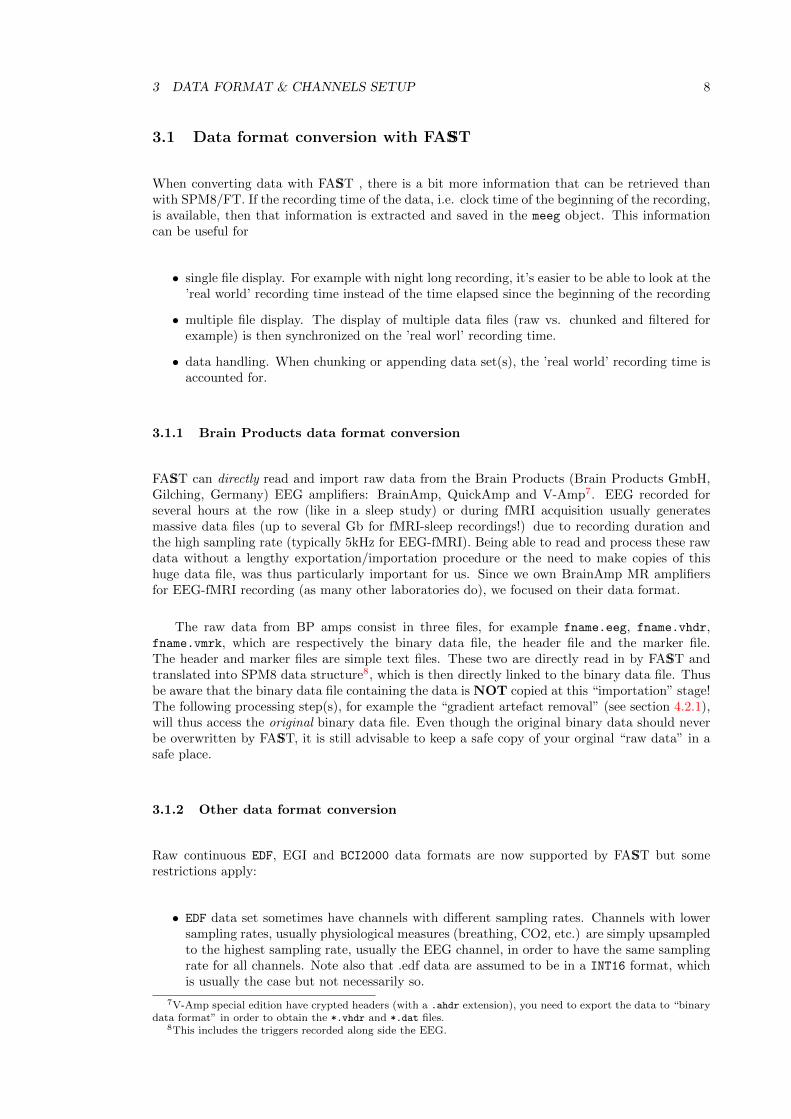
3.1 Data format conversion with FASST
When converting data with FASST , there is a bit more information that can be retrieved thanwith SPM8/FT. If the recording time of the data, i.e. clock time of the beginning of the recording,is available, then that information is extracted and saved in the meeg object. This informationcan be useful for
• single file display. For example with night long recording, it’s easier to be able to look at the’real world’ recording time instead of the time elapsed since the beginning of the recording
• multiple file display. The display of multiple data files (raw vs. chunked and filtered forexample) is then synchronized on the ’real worl’ recording time.
• data handling. When chunking or appending data set(s), the ’real world’ recording time isaccounted for.
3.1.1 Brain Products data format conversion
FASST can directly read and import raw data from the Brain Products (Brain Products GmbH,Gilching, Germany) EEG amplifiers: BrainAmp, QuickAmp and V-Amp7. EEG recorded forseveral hours at the row (like in a sleep study) or during fMRI acquisition usually generatesmassive data files (up to several Gb for fMRI-sleep recordings!) due to recording duration andthe high sampling rate (typically 5kHz for EEG-fMRI). Being able to read and process these rawdata without a lengthy exportation/importation procedure or the need to make copies of thishuge data file, was thus particularly important for us. Since we own BrainAmp MR amplifiersfor EEG-fMRI recording (as many other laboratories do), we focused on their data format.
The raw data from BP amps consist in three files, for example fname.eeg, fname.vhdr,fname.vmrk, which are respectively the binary data file, the header file and the marker file.The header and marker files are simple text files. These two are directly read in by FASST andtranslated into SPM8 data structure8, which is then directly linked to the binary data file. Thusbe aware that the binary data file containing the data is NOT copied at this “importation” stage!The following processing step(s), for example the “gradient artefact removal” (see section 4.2.1),will thus access the original binary data file. Even though the original binary data should neverbe overwritten by FASST, it is still advisable to keep a safe copy of your orginal “raw data” in asafe place.
3.1.2 Other data format conversion
Raw continuous EDF, EGI and BCI2000 data formats are now supported by FASST but somerestrictions apply:
• EDF data set sometimes have channels with different sampling rates. Channels with lowersampling rates, usually physiological measures (breathing, CO2, etc.) are simply upsampledto the highest sampling rate, usually the EEG channel, in order to have the same samplingrate for all channels. Note also that .edf data are assumed to be in a INT16 format, whichis usually the case but not necessarily so.
7V-Amp special edition have crypted headers (with a .ahdr extension), you need to export the data to “binarydata format” in order to obtain the *.vhdr and *.dat files.
8This includes the triggers recorded along side the EEG.

4 MAIN FUNCTIONS OF THE TOOLBOX 9
• EGI data should be continuous “raw exported” data. For the moment, the data file is readin and re-written on disk after removing the channels associated with the triggers/inputs9.These trigger/inputs are turned into events in the SPM8 meeg object.
• BCI2000 data importation is only a beta version!
As stated above, other (raw) EEG/MEG data formats should be imported via SPM8 importationroutine. In this case the raw binary file is copied and the 2 files created (*.mat and *.dat) areprepended with “spm8 ”.
3.2 Channel definition
Channel definition (name, type, sacele, unit, 2D-location, etc.) is in line with that of SPM8.Therefore it is strongly advisable to use SPM8’s review function to set up the channel informa-tions properly and, possibly, apply a montage to re-reference all or some channels. Still within thetoolbox we use an enhanced “channel setup” file (CRC electrodes.mat) specific to EEG record-ings, and introduce an extra bit of information “crc types” for the channels. This allows theon-the-fly display of bipolar montage along EEG channels and the use of different channel scal-ings, e.g. for EEG and ECG channels, for the display. Most common channel names are alreadyavailable within the toolbox. If you used a lab-specific setup (and most everyone does...) or weirdchannel names, you should then add those channels to CRC electrodes.mat. For more infor-mation on how to adjust the channel definitions to your specific channel setup, please read andedit the function crc electrodes.m. A new CRC electrodes.mat is then generated by executingcrc electrodes.m.
4 Main functions of the toolbox
The following tools and features are available in the current version of FASST:
• General tools
– Displaying one M/EEG data file
– Comparing multiple M/EEG data files
– Appending M/EEG data files into a single data file
– Chunking a time window from an M/EEG data file
– Computing the spectrogram of one M/EEG data file
– Displaying the spectrogram or power spectrum of an M/EEG data file
• EEG-fMRI artefact rejection tools
– Gradient artefact rejection: AAS method
– Pulse artefact rejection: AAS, ‘Gaussian mean’ and cICA methods
9It should be possible though to avoid reading-and-writing the big data file on disk and directly access theoriginal raw data. Maybe in a future update...
4 MAIN FUNCTIONS OF THE TOOLBOX 10
• Sleep specific tools
– Manual sleep scoring
– Spectral power calculations and statistics
• Automatic wave detection tools
– Slow waves (SW)
– sleep spindles (SP, beta version)
4.1 General tools
These are tools to display, review, compare, process, manipulate and handle (long) multichannelcontinuous data files.
4.1.1 Displaying one M/EEG data file
This tool is designed to display multiple channels of one continuous M/EEG recording and browsethroughout the data. The display routine includes built-in “on-screen” filtering and re-referencingfunction. There is therefore no need to perform these pre-processing steps before visualizing thedata. In fact you can use these options to see what would be the effect of filtering or re-referencingon your data.
When you launch the display routine, the selection channel interface appears first. At thispoint you have to choose the list of channels you want to look at. To select a channel, you just haveto click on its name in the left hand column (Fig. 2-A). The name of this channel will disappearfrom the left column and appear in the right column (Fig. 2-B). The channels recognized by thetoolbox, i.e. with 2D-localisation information, will appear in the lower right white box (Fig. 2-C)according to their position on the scalp. Some buttons allow you to automatically select a setof electrodes (Fig.2-D). When you have selected all the channels of interest, click on the ‘PLOT’button to launch the display interface (Fig. 2-E). The ‘SCORE’ button (Fig. 2-F) leads to thesame display but with the scoring tools and menu enabled, see section 4.3.1.
A display window appears with the channel display in the main central box (Fig. 3-A). Thescaling, time window settings, number of channels displayed, re-referencing and filtering optionare on the right part of the window (Fig. 3-B). There are two scrolling bars: one to quickly browsethroughout the data over time, below the channel display (Fig. 3-C), and another one to browsethrough sub-sets of selected channels, on the right of the channel display (Fig. 3-D).
In the main display window (Fig. 3-A), standard unipolar channels are displayed in darkblue, electrocardiographic (EKG or ECG) in red and the others in lighter blue. The scaling ofthe various channels will depend on their type, as defined in the SPM8 meeg object. If thisinformation is not available (poor importation or the data have not been “properly” prepared)then FASST uses the crc types variable of the channel setup file crc channels.mat to find thechannels that are automatically rescaled and the bipolar montages10.
10In this case, it will not be possible to scale correctly EEG and MEG channels simultaneously!

4 MAIN FUNCTIONS OF THE TOOLBOX 11
Figure 2: Channel selection GUI: A. channel list, B. selected channels, C. selected channels 2D-location, D. pre-specified automatic channel selection, E. plot selected channels, F. plot selectedchannels and score the signal.
The ‘Window Size’ (Fig. 3-B1) fixes the length of the window displayed (in seconds). The‘Scale’ setting fixes the relative distance in µV between two channels in the main window (Fig. 3-B2). The number between two channel labels stands either for minus half the scale for the abovechannel and for plus the half scale for the lower channel. This scale indicates a signal of referencein the order of 150µV . Channels with other units will be rescaled according to their type (seethe ‘Scales’ pull-down menu (Fig. 3-K), while the ‘Scale’ value (Fig. 3-B2) will act on the signalof all channels at once. For example if you fixed the scale at 150 µV , 75 will appear betweenlabel channels and the scale of each EEG channel goes from -75 µV to +75 µV . The ‘Number ofdisplayed channels’ (Fig. 3-B3) fixes the number of channels per screen (to see the other channles,scroll up or down).
The ‘Reference’ panel (Fig. 3-B4) allows you to re-reference the data to a chosen reference.For the EEG channels, this reference may be any other channels (even if you did not select itin the channel selection interface), the mean of all the EEG channels or the mean of the twomastoids (called M1 and M2). For the EOG and EMG channels you have an additional ‘Bipolar’choice for the reference. Pairs of EOG (and EMG) channels are usually designed to work as abipolar montage, let’s say that EMG1 and EMG2 are specified to be referenced to each other. Ifyou only display EMG1 and choose the bipolar reference, then EMG1 will be displayed referencedto EMG2. Note that this re-referencing relies on the channel names and is performed only ‘on-display’ (the original data stored on disk are left untouched).
The ‘Filter’ panel (Fig. 3-B5) allows you to bandpass filter the various types of channelsdifferently. The cut-off frequencies are indicated in the boxes next to the channel type. Like there-referencing, this filtering is performed only ‘on-display’ and the original data stored on diskare left untouched.
The ‘Save Position’ button (Fig. 3-F) allows you to store the time your time cursor is currentlyat and, when opening the same file later, your time cursor will be replaced at that position. Usefulwhen reviewing waves or when scoring very long files. The ‘Score Sleep’ button (Fig. 3-G) allowsyou to launch the scoring utility to score the file you are currently displaying. The ‘View another

4 MAIN FUNCTIONS OF THE TOOLBOX 12
Figure 3: Channels display window: A. main display, B. display options (see text for details),C. time scrolling bar, D. go to sleep scoring, E. view another file, F. back to channel selection,G. time in seconds at the beginning of display, H. export display to a Matlab figure.
file’ button (Fig. 3-H) allows you to select another file to display and, eventually, the ‘Back tochannel selection’ button (Fig. 3-I) lets you go back to the channel selection interface.
The box below the time-slider shows the current time (Fig. 3-J), in the middle of the displaywindow, expressed in seconds, from the beginning of the recording; the other number is the overalllength of the recording also expressed in seconds. You can type in a value to jump directly toany moment of interest in the recording.
Events comprised in the data set are displayed as small triangles on the display. The ‘events’panel (Fig. 3-E) allows to scroll through these events, by first choosing which events type andvalue to display (respectively the left and right pull-down menus) and then using the ‘previousand ‘next’ buttons to move to the nearest previous and next event. The events types and valuesare those saved in the events field of the data.
For the case where waves (e.g. slow waves or sleep spindles) were automatically detected (seesection 4.4), some specific codes are used:
• for spindles, the event type would be ‘spindles’, ‘Post-SP’ or ‘Ant-SP’, with code values of777, 666 or 555 respectively. ’spindles’ are marked when no wavelet analysis is used duringdetection, otherwise they are differentiated into posterior or anterior spindles (‘Post-SP’and ‘Ant-SP’ respectively).
• For slow waves, the event types are either ‘SW’ (codes starting with 3) or ‘delta’ (codestarting with 4).
4 MAIN FUNCTIONS OF THE TOOLBOX 13
The ‘events number’ option from the right pull-down menu lets you display the values of theselected events instead of their type11. Using the ‘good event’ radio button, individual events canbe marked as good (by default, value 1) or bad (0). Events marked as ‘bad’ appear in red on thedisplay. The good/bad values of all events are saved in a new ‘goodevents’ field specific to FASSTin the meeg object. For spindles and slow waves particularly, the values are also saved in the‘spindles’ and ‘SW’ fields, created when detecting the waves. Note that any change in the eventnumbering or any new wave detection will overwrite this information12. Finally, when displayinga slow wave, a ‘map of delay’ radio-button will be visible. When checked, a propagation mapof the current SW (based on the SW delay) is displayed. The 2D channel location either comesfrom default CRC channels positions (‘auto’) or the positions of your channels (‘file’, then selectyour file).
A series of pull-down menus are available in the upper part of the main display window(Fig. 3-K). There is a button allowing you to export the current plot to a new Matlab figure.This may be handy if you plan to save the displayed signal as an image file. Next to this menu,a ‘Scales’ menu is also available, letting you enter directly the scale of certain types of channels:defined as 10x, with x representing the factor of your signal of interest compared to your originaldata. For example, if you have EEG channels recorded in Volts (V), the scale should be 10−6,since the signal of interest is in µV .
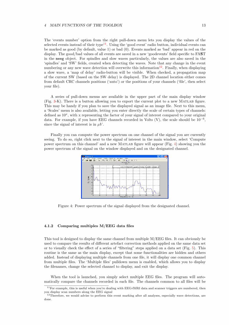
Finally you can compute the power spectrum on one channel of the signal you are currentlyseeing. To do so, right click next to the signal of interest in the main window, select ‘Computepower spectrum on this channel’ and a new Matlab figure will appear (Fig. 4) showing you thepower spectrum of the signal on the window displayed and on the designated channel.
Figure 4: Power spectrum of the signal displayed from the designated channel.
4.1.2 Comparing multiples M/EEG data files
This tool is designed to display the same channel from multiple M/EEG files. It can obviously beused to compare the results of different artefact correction methods applied on the same data setor to visually check the effect of a series of “filtering” steps applied on a data set (Fig. 5). Thisroutine is the same as the main display, except that some functionalities are hidden and othersadded. Instead of displaying multiple channels from one file, it will display one common channelfrom multiple files. The ‘Multiple files’ pulldown menu is enabled, which allows you to displaythe filenames, change the selected channel to display, and exit the display.
When the tool is launched, you simply select multiple EEG files. The program will auto-matically compare the channels recorded in each file. The channels common to all files will be
11For example, this is useful when you’re dealing with EEG-fMRI data and scanner triggers are numbered, thenyou display scan numbers along the EEG signal
12Therefore, we would advise to perform this event marking after all analyses, especially wave detections, aredone.

4 MAIN FUNCTIONS OF THE TOOLBOX 14
available for display. Only one channel can be displayed at one time. The displayed channel canbe modified via the ‘Multiple files’ menu.
The routine also checks the beginning time of each recording (if available) and aligns thedifferent EEG time series in consequence. If the beginning time was not imported from the rawdata (or was manually deleted at some point), it is assumed that all files begin at the same time:their first time bin. Otherwise the “true” beginning time of each file is used: if for some timewindow, some signal is missing from one data set (e.g., you chunked out the 1st few seconds of adata set before filtering it) then that data channel is left empty.
Figure 5: Multiple files comparison GUI, with some features from the main display GUI andothers specific to this data comparison GUI.
Contrary to the colour scheme of the main display tool, here the different files are simplydisplayed in different colours to differentiate them. If you right-click on the displayed signal, youmay display the power spectrum of the displayed channel for one or all of the signals currentlydisplayed .
4.1.3 Appending M/EEG data files
Sometimes during long recording session, the operator may need to stop the recording to fixsome problem, or recording may be accidentally interrupted. So for one “recording session”, theuser ends up with two (or sometimes more...) EEG files. This tool is designed to append thoseseparate EEG files into a single one.
The routine works with two files at a time. So when you have more than two files, you shouldappend the first two files which creates a new file that you append with the third, and so on:
• If the ’real world’ recording time of each file is available, the routine first checks the ’realworld’ begining time of each file, and automatically determines the file order. Then it fillsthe gap between the end of the first data set and the beginning of the second by zero’s, andeventually appends the second the file.

4 MAIN FUNCTIONS OF THE TOOLBOX 15
• If no ’real worl’ time information is available in the file (after using the SPM8/FT conversionfor example), the routine will ask if you want to operate a ‘blind concatenation’. In thiscase, the routine supposes that there is no missing samples between the consecutive file andthat you entered the files in the correct order.
In both cases, the resulting file has the same name as the first file selected prefixed with cc .
4.1.4 Chunking a time window from an M/EEG data file
This tool allows the user to cut out an episode out of a large EEG file and save it as a differentEEG file. This can be useful if one wants to study specific activity such as sleep stages, epilepticdischarge,... The beginning and end of the new file can be defined by a marker or by time (Fig. 6).
Figure 6: Chunking tool GUI.
If the user chooses the time option, he will have to choose between “Relative time” (timefrom the beginning of the file) and “Clock time” (the real world recording time). If the userchooses marker, he will have first to choose which type of marker to use (each type of marker hasa different ‘label’) and next, the index of the marker. For example, one can use the type marker0 and choose the 1st marker, i.e. the index will be 1.
The end of the file is fixed in the same way. When the desired parameters are entered for thebeginning and end of the chunk, the user may press the ‘Chunk!’ button to perform the chunking
4.1.5 Computing the spectrogram of one M/EEG data file
This routine computes the spectrogram, using the Welch periodogram method, of the selectedfile according to parameters specified by the user. The result is saved into a time-frequency datafile. Note that this file is not in a true SPM8 meeg object format: it is saved as a seperatefile array data formtat, stored in the meeg object structure. Before the computation itself, thedata are filtered (bandpass filter between 0.5 and 25 Hz by default, Fig. 7-A). The spectrogramis computed over time windows (of 4s by default, Fig. 7-B) every time steps specified by the user(2 by default, Fig. 7-C).
If the file was scored using the scoring tool (see section 4.3.1), the sections scored as movementtime or marked as artefacts are left out of the spectrogram calculation (power is set to zero). Ifthe file was scored by multiple users, the score to be used is selected via the pull-down menu

4 MAIN FUNCTIONS OF THE TOOLBOX 16
Figure 7: Spectrogram calculation GUI: A. band-pass filtering, B. time window, C. time step,D. scorer selection (if available), E. reference channel, F. launch calculation.
(Fig. 7-D). The artefacted, ‘movement’ or ‘unscorable’ periods are displayed on the spectrogramby blue lines, the width depending on the duration of the arefact, movement/unscorable period.On the frequency band display, the display is just blank at those periods.
The last parameter is the reference taken for the computations (Fig. 7-E). Once all theparameters have been fixed the user may click on the ‘Compute spectrogram’ button (Fig. 7-F).When the computation is complete, a “.frq” file containing the spectrogram is available, and thefile array information (as well as the calculation parameters) are stored in the D.CRC.pwrspectsubstructure.
4.1.6 Displaying the spectrogram or power spectrum of an M/EEG data file
This tool is designed to display the spectrogram computed by the ‘Compute spectrogram of oneEEG file’ (cfr. section 4.1.5). Two display modes are available (Fig. 8-A): “Spectrogram” and“Frequency band”. “Spectrogram” is a time-frequency representation of one channels, dark bluerepresenting low power and bright-red, higher power. A pull-down menu, Fig. 8-B, is used toselect the channel to display.
In the “Frequency band” display mode, the evolution of the power in a specified frequencyband (Fig. 9-D) is displayed for one or two channels (channels are picked using 2 pull-down menus,Fig. 9-A). In this display mode, three scaling modes are available (Fig. 9-B): “Absolute value”;“Relative value”, i.e. how much power is dissipated at time t in the considered band dividedby the whole power at time t; and the “Mongrain view” (usually used by sleep specialist), itshows the power dissipated at time t in the selected frequency band divided by the mean powerin deep sleep stage during the night. Once the scaling mode chosen, the scale itself can be fixed(Fig. 9-C).
Right clicking on the main plot (either the spectrogram or the frequency band display) letsyou define ‘Periods of Interests’ (POI), which will be saved in a new freq POI field in the datastructure, as well as in a text file, along the data set. Periods of Interest are defined in the sameway as artefacts in the scoring option: the user defines a start and an end points, which relativetimes are saved in the data set in seconds. The absolute (if available) or relative times in thehh-mm-ss format of all POIs can be displayed in a new figure using the ‘POI info’ option of theright-click menu. POIs can be deleted by right-clicking on the vertical lines defining either theirstart or end points.
If the file was previously scored (see section 4.3.1), the hypnogram is also displayed (Fig. 9-E).The user may choose which score to use, and compute the mean power spectrum during a specificsleep stage (Fig. 9-F, results are shown in Fig. 10).

4 MAIN FUNCTIONS OF THE TOOLBOX 17
Figure 8: Main display of spectrogram GUI, “spectrogram display”: A. display mode toggle,B. channel selection.
4.2 EEG-MRI artefact rejection tools
In this section we describe the fMRI artefact rejection tools. When EEG is recorded in a MR scan-ner during image acquisition (typically fMRI), two types of artefacts are induced on top of theneural EEG signal:
• The Gradient Artefact (GA) is induced by the gradient switching of the imaging sequenceof the MR scanner[?]. Note that this several order of amplitude larger than the genuineEEG signal.
• The Pulse Artefact (PA) is due to the interaction between the static field of the MR scannerand the heartbeats[?]. Note that this artefact is thus present even if no fMRI data areacquired.
One should always suppress the gradient artefact before the pulse artefact.
4.2.1 Gradient artefact rejection
This tool allows the user to remove the Gradient Artefact (GA) resulting from the gradientswitching of the MR acquisition sequence. The removal method is based on the “Average ArtefactSubtraction” (AAS) method developed by Allen et al.[?]. AAS estimates the shape of the GAover a TR (the time to acquire a fMRI volume) by averaging the signal over several (typicallyat least 10) contiguous MR volume acquisitions. This “averaged artefact” is estimated for eachTR and subtracted from the recorded EEG signal. The efficiency of the AAS approach relieson the stationarity of the GA picked in the EEG signal. This stationarity can be enforced bysynchronizing the clocks of the EEG amplifier(s) with that of the MR scanner. This is a crucial

4 MAIN FUNCTIONS OF THE TOOLBOX 18
Figure 9: Main display of spectrogram GUI, “frequency band display”: A. channel(s) selection,B. scaling type, C. scale for display.
point and any user applying this algorithm on data acquired without clock synchronization may(and most certainly will) have improper GA rejection.
This tool is quite simple to use: just select the file(s) you want to correct for gradient artefact.For each file selected, a “wait bar” shows you the evolution of the correction and a new data fileis (slowly) generated. After corrections your corrected files have the same name as the originalones prefixed with cga and are available for further processing. The parameters of the gradientrejection are located in the crc defaults.m file which you should edit in order to make theprogram compatible with your specific MR sequence specification and amplifier setup.
There are 2 options to detect the beginning of each scan:
• if you record markers coming directly from the scanners to indicate the beginning of eachvolume (or slice) acquisition, then set the variable crc defaults.gar.UseScanMrk to 1.You then have to specify the type of marker you are using in crc defaults.gar.ScanMrk1
(for example crc defaults.gar.ScanMrk1 = 12813). If you use slice markers, i.e. onetrigger from the scanner every slice, rather than volume marker, you have to set thecrc defaults.gar.MrkStep as the number of slices composing a volume.
• If you do not record the triggers coming from the scanner (slice or volume) to define the be-ginning of each volume, set the variable crc defaults.gar.UseScanMrk to 0. You then haveto specify the exact TR of your sequence in seconds (crc defaults.gar.TR field). You mayautomatically detect the beginning and end of the scanning episode in the EEG file using anautomatic check(field crc defaults.gar.Autochk = 1). You can also manually specify the beginning andend of the scanning sequence (crc defaults.gar.beg and crc defaults.gar.nd).
13A secondary marker type can be specified in the field crc defaults.gar.ScanMrk2.

4 MAIN FUNCTIONS OF THE TOOLBOX 19
Figure 10: Mean power spectrum during a specific sleep stage (stage 2) for one channel (Oz here).
The sampling frequency of the original file (typically 5kHz) is usually higher than neces-sary for further processing, you can thus specify the sampling frequencey of the output file incrc defaults.gar.ouput fs (500Hz by default). The other parameters specify the prefix addedto the filename for the corrected file (crc defaults.gar.prefix), the number of scan on whichthe average is performed for artefact rejection (crc defaults.gar.Nsc aver) and the number ofscans skipped at the beginning of the scanning sequence(crc defaults.gar.Nsc skipped be). Note that the corrected data saved will start at the be-ginning of the 1st corrected TR, i.e. any pre-scan data are omited. If you’re interested in thesignal prior that point, then you should extract it (see section 4.1.4) from the uncorrected fileand possibly append it afterwards (see section 4.1.3).
4.2.2 Pulse artefact rejection
This tool allows the user to reject the “Pulse Artefact” (PA) in the EEG recordings. This artefactis induced by the heartbeats of the subject lying in the static field of the MR scanner and is thuspresent even if no MR data are acquired.
When the tool is launched, the user has to choose which channels will be corrected. Usu-ally EMG or ECG channels are not selected for correction. This step is crucial for ICA-basedmethods. ICA-based methods are multi-channel methods, i.e. the signal from all the channelsare considered together, therefore, if inappropriate (ECG/EMG-like) channels are selected, someEMG information might contaminate EEG data after an ICA-based correction. So you shouldalso ensure that any bad channel(s) are left out from the pulse artefact correction process as theycould confuse the ICA-based methods.
Once you have selected the channels to correct for each file, you choose the ECG peak detectionmethod. At the moment the only available method is the one developed by R. K. Niazy andreferred to as “the FMRIB plug-in for EEGLAB”, provided by the University of Oxford Centrefor Functional MRI of the Brain (FMRIB) [?]. We found it very robust even on relatively noisyECG channels.
After this step, you can choose the type of pulse artefact rejection method you will use. Thereare five of them: “PCA” (FMRIB plug-in), “Gaussian mean” (AAS from FMRIB plug-in) [?, ?],“constrained ICA (automatic)”, “constrained ICA (manual)” [?] and “AAS & PCA combined”

4 MAIN FUNCTIONS OF THE TOOLBOX 20
(based on the FMRIB plug-in)14. The last step lets you choose which channel number is theECG. If you leave 0, the algorithm will automatically detect it.
Constrained-ICA method. Be aware that long episodes with movement artefacts can com-promise cICA correction. Indeed cICA works on one time-window (90 seconds by default) ata time and episodes showing “movement activity” are not used for the correction estimate (seeparameter crc defaults.par.bcgrem.scSNR here under). So if there is proportionally too muchmovement during a time-window, not enough “good” signal will be available and cICA will not beable to properly decompose the recorded signal and reject the pulse artefact. If you see messagesin Matlab command window such as
Rejecting more than 50% of time bins from current time window!
Warning: Algorithm fails to correct the EEG recordings, probably due to’
too much artefacts.
You should worry about your data: either the gradient artefact rejection did not work so welland your data are still too noisy, or there are some ‘bad’ channels and you should exclude themfrom the cICA corrections.
Since a seperate cICA correction matrix is estimated and saved for every 90 second timewindow, it is possible to replace ‘bad’ ones by a better one. The selection of the optimal cICAcorrection matrix can be automatic (option “constrained ICA (automatic)”) or manual (option“constrained ICA (manual)”):
• With the automtaic approach a ‘mutual information’[?] criteria is used to decide whichcICA correction matrix to use: Let’s define 2 mutual information measures MI1 and MI2like this: MI1 = MI(original data, AAS artefact template) and MI2 = MI(corrected data,AAS artefact template). Then the cICA correction matrix leading to the smallest ratioMI2/MI1 is deemed optimal. The MI measures are estimated from random samples of datain the data set, as specified in crc defaults.par.useinitseg, .additioseg and .length.Then the corrected data are saved on disk as a new data set.
• With the manual approach, no corrected data are saved on disk and the user must decidewhich correction matrix(-ces) to employ. This selection is performed via the usual displayfunction (see section 4.1.1) and the user can directly visualize the corrected signal obtainedby any saved cICA correction matrix. Once the cICA correction matrix is selected, thecorrected data are generated and saved on disk in a new data file.
AAS, PCA and other methods. We would advise users with 30 channels or more to choosea “constrained ICA” (cICA) method. cICA was shown to be more efficient than AAS and PCAat rejecting the PA and to better preserve the spectrum of the “true” EEG signal [?]. This isparticularly important when analyzing the time course of spontaneous activity (such as in sleepstudies).
With fewer channels (<30) or lots of movement activity, single-channel methods are bettersuited. “Gaussian mean method” (AAS)is often preferable but PCA can also do a good job. The“AAS & PCA combined” method is experimental and has not been rigorously tested. During the
14a “multi ICA” approach [?] is also available but not throught the GUI as it takes far too much time to calculateand has not been extensively validated

4 MAIN FUNCTIONS OF THE TOOLBOX 21
preparation of [?], we noticed that AAS was more efficient for the lower part of the data spectrumand PCA for the higher part15. “AAS & PCA combined” thus uses a combination of AAS andPCA: AAS is applied on the low-pass filtered (<4Hz) signal and PCA on the high-pass filtered(>4Hz) signal, then the 2 corrected parts are recombined afterwards.
Specific options. Users are in effect advised to test test correction methods and find out the“best” one for their own data. In crc defaults.par.bcgrem, you can change some parameterslinked to the PA rejection, but most of these concern the constrained ICA method such as
.size the window size (in seconds) on which cICA is performed;
.step the step between the beginning of two windows;
.scSNR the number of standard deviation signal must deviate from to be considered as “noise”or “movement”, i.e. to be exluded from the cICA estimation;
.Refnames the channels representative of the shape of the pulse artefact;
.NitKmeans the number of iteration of the K-means step.
4.3 Sleep specific tools
These tools and GUI’s were specifically developed for sleep data analysis, like the manual scoringof sleep M/EEG (section 4.3.1). The power spectrum of scored data can be estimated anddisplayed. Finally some summary statistics, about sleeping time, sleep stage duration, etc., canalso be calculated afterwards. The spectral power through some sleep stages can also be estimated(section 4.3.2).
You can also automatically detect some sleep patterns in your file. This version of FASSTdeals with ‘Slow Waves’ (section 4.4.1) and ‘Sleep Spindles’ (section 4.4.2)16.
4.3.1 Manual sleep scoring
Once the user has selected the file to score, the selection channel interface appears (same interfaceas in section 4.1.1). Once you have selected your favourite channels, hit the ‘Score’ button.
The main display then appears, with all scoring related tools enabled. In particular, a ‘Scor-ing’ pulldown menu is now visible on the top left of the window. With this menu, you are able tochoose the scorer or define another scorer, compare scores, import scores or display grids (verticalevery second or horizontal at half of the main scale). Since this is a scoring tool the size of thedisplayed time-window is fixed and cannot be changed once it is chosen.
If the file is scored for the first time, the program asks a username and a window size. Thesame file may be scored by different users. To introduce a new scorer, the user has to select “Newscorer” at the bottom of the scorers option of the ‘Scoring’ menu.
15In particular, slow waves were sometimes removed by the PCA methods16this latter part of the code is in beta version.

4 MAIN FUNCTIONS OF THE TOOLBOX 22
Figure 11: Sleep scoring GUI, with the hypnogram display on top of the the EEG signal.
The keypad is used to assign a score to the current window. Each number correspondsto a specific stage17. By default these are set as: “Wakefulness” (0), “Sleep stage 1-4” (1-4respectively), “REM sleep” (5), “Movement Time” (6), and “Unscorable” (7). Each time a scoreis assigned to the current window, the display moves on to the next time-window. The letters“b” and “f” can be used to move backward and forward by one time window without assigningany score to the current window. During scoring a hypnogram is automatically constructed and atick mark shows the current position in the signal. Note that to score a window the main displaywindow has to be selected (i.e. clicked in).
The right-click menu allows the user to add 4 types of events:
• “artefact & arousal”, which will be considered as artefact for power spectrum computation,cfr. section 4.1.5. Artefacts can be defined in two ways: either as ‘unspecified’ artefacts oras ‘specified’ artefacts. This last option allows to choose a label for the manually definedartefacts, amongst common categories of artefacts (i.e. blink, eye movement, movement).When selecting an unspecified artefact, the label associated to that artefact will be leftempty. It is therefore possible to define specified and unspecified artefacts in the samescore18. When defining an artefact (or arousal resp.), the background color of the plot willbe changed from white to light blue (light red resp.) to avoid opening an artefact (arousalresp.) without closing it.
• “event of interest”. This generic event can be used in different ways depending the interestof the user: for example to manually mark spindles, epileptic discharge,...
• “FPL marker”, i.e. “closing door & light” marker (in French “Fermer Porte & Lumiere”),to indicate the beginning of the night of recording.
• ‘OPL marker”, i.e. “opening door & light” marker (in French “Ouvrir Porte & Lumiere”),to indicate the end of the night of recording.
17The labels can be modified in the default file but NOT their number, which is hard coded in some routines.18Labels can then be found in the 8th row of the score field created in the data set.

4 MAIN FUNCTIONS OF THE TOOLBOX 23
The latter two, FPL and OPL markers are important to compute sleep statistics. Artefacts,arousals and events of interest are marked as crosses (respectively grey, red and dark red crosses)on the hypnogram to allow a global visualisation of them along the night.
4.3.2 Spectral power calculation and statistics
The last item of the right-click pulldown menu is the compute power spectrum tool, same asin section 4.1.1. These tool are exactly the same as those described in sections 4.1.5 and 4.1.6.If the file was scored using the sleep scoring function, the sections scored as movement time ormarked as artefacts are left out of the spectrogram calculation (power is set to zero). If the filewas scored by multiple scorers, the user has to decide which score to use (Fig. 7-D).
The hypnogram is also displayed (Fig. 9-E) alongside the spectrogram display. The user maychoose which score to use, and compute the mean power spectrum during a specific sleep stage(Fig. 9, results are shown in Fig. 10).
Finally the ‘Compute Statistics’ button is accessible via the ‘Scoring’ pull-down menu: theproportion of the different sleep stages, of the movement time and of the wakefulness stage, thelatency of REM sleep, etc. are then displayed (Fig. 12).
Figure 12: Sleep statistics results.
4.4 Automatic wave detection tools
Automatically extrating features from continuous EEG recording is a complicated task mainlybecause of the poor signal-to-noise ratio and the variability (within and between subjects) of the“waves” to detect. We focused on two types of spontaneous sleep waves, namely “slow waves”and “spindles”. The methods are described in the next two sections. Still, when using these tools,keep in mind that wave detection is not “bullet proof” and paramter may need to be tweaked toachieve the best results on your data.
4 MAIN FUNCTIONS OF THE TOOLBOX 24
4.4.1 Slow Wave detection
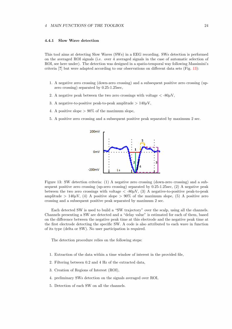
This tool aims at detecting Slow Waves (SWs) in a EEG recording. SWs detection is performedon the averaged ROI signals (i.e. over 4 averaged signals in the case of automatic selection ofROI, see here under). The detection was designed in a spatio-temporal way following Massimini’scriteria [?] but were adapted according to our observations on different data sets (Fig. 13):
1. A negative zero crossing (down-zero crossing) and a subsequent positive zero crossing (up-zero crossing) separated by 0.25-1.25sec,
2. A negative peak between the two zero crossings with voltage < -80µV,
3. A negative-to-positive peak-to-peak amplitude > 140µV,
4. A positive slope > 90% of the maximum slope,
5. A positive zero crossing and a subsequent positive peak separated by maximum 2 sec.
Figure 13: SW detection criteria: (1) A negative zero crossing (down-zero crossing) and a sub-sequent positive zero crossing (up-zero crossing) separated by 0.25-1.25sec, (2) A negative peakbetween the two zero crossings with voltage < -80µV, (3) A negative-to-positive peak-to-peakamplitude > 140µV, (4) A positive slope > 90% of the maximum slope, (5) A positive zerocrossing and a subsequent positive peak separated by maximum 2 sec.
Each detected SW is used to build a “SW trajectory” over the scalp, using all the channels.Channels presenting a SW are detected and a “delay value” is estimated for each of them, basedon the difference between the negative peak time at this electrode and the negative peak time atthe first electrode detecting the specific SW. A code is also attributed to each wave in functionof its type (delta or SW). No user participation is required.
The detection procedure relies on the following steps:
1. Extraction of the data within a time window of interest in the provided file,
2. Filtering between 0.2 and 4 Hz of the extracted data,
3. Creation of Regions of Interest (ROI),
4. preliminary SWs detection on the signals averaged over ROI,
5. Detection of each SW on all the channels.
4 MAIN FUNCTIONS OF THE TOOLBOX 25
Once the SWs are detected, the trajectory of the peak negativity over the scalp surface is alsoextracted using the information from all channels (SW detection and channel location). Finallythe SWs are displayed.
The characteristics of the detected waves are saved in a new field D.CRC.SW of the originaldata structures19. Their most important characteristics are also saved in the field D.events toallow an easy epoching of the waves. This new field D.CRC.SW is also saved in the chunked andSW files if the option in ‘Analyse’ was not ‘all file’. In that case, the time characteristics of thewaves will be relative to the start of the input file in its SW field while they will be relativeto the start of the chunked or SW file in theirs. This allows using either the input file or thechunked/SW file for SW analysis, according to what suits your needs best.
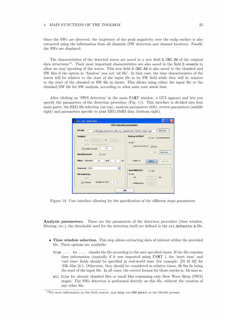
After clicking on ‘SWS detection’ in the main FASST window, a GUI appears and lets youspecify the parameters of the detection procedure (Fig. 14). This interface is divided into fourmain parts: the EEG file selection (on top), analysis parameters (left), review parameters (middleright) and parameters specific to joint EEG-fMRI data (bottom right).
Figure 14: User interface allowing for the specification of the different steps parameters
Analysis parameters. These are the parameters of the detection procedure (time window,filtering, etc.), the thresholds used for the detection itself are defined in the crc defaults.m file.
• Time window selection. This step allows extracting data of interest within the providedfile. Three options are available:
from ... to .... chunks the file according to the user specified times. If the file containstime information (typically if it was imported using FASST ), the ‘start time’ and‘end time’ fields should be specified in real-world time (for example, [23 45 02] for‘23h 45m 2s’). Otherwise, they should be considered as relative times, 0h 0m 0s beingthe start of the input file. In all cases, the correct format for those entries is: hh-mm-ss.
all file for already chunked files or small files containing only Slow Wave Sleep (SWS)stages. The SWs detection is performed directly on this file, without the creation ofany other file.
19For more information on this field content, type help crc SWS detect at the Matlab prompt.

4 MAIN FUNCTIONS OF THE TOOLBOX 26
sheets scored builds a new file from the concatenation of all sheets scored ‘scores’ (spec-ified by spaced numbers, e.g. 3 4). This new file is stored on the drive under thename SW filename. This option is particularly useful if there is no specific momentof interest in the file: if the input file is a whole night recording and by specifying thescores as 3 and 4, the SWs detection will be performed on all SWS stages.
Note that, in all cases, periods marked as artefacted (artefacts or arousals) or as movementtime or unscorable will be skipped from the analysis.
• Re-reference parameters. The algorithm checks for a re-referencing operation in the fieldD.history (modified after each SPM8 processing). If it does not find such an operation,the user is asked if he wants to continue or not. Please, apply your montage before anyprocessing of the data.
• Filter parameters. If the file wasn’t filtered in the frequency band of interest, the proce-dure will band-pass filter the data (by default, 0.2-4Hz) by applying first a 0.2Hz highpassfilter and then a lowpass filter with cutoff frequency at 4Hz to ensure stability. No files arecreated from this operation. If such filtered files are useful for you, you should preferablyfirst filter the data in SPM8 and specify the newly created file as input. The filters usedare the same as those of SPM8 (Butterworth type) 20.
• Scorer Pull down menu. To choose the scorer’s score to use.
• ROI selection parameters. To decrease the computational load, SWs detection is firstperformed on averaged signals over (typically) 4 ROIs: frontal, central left, central rightand parietal. Two options are available for the channel selection:
automatic Channels in a radius (below about 15% of scalp radius) around the 2D normal-ized flattened positions of respectively Fz, C3, C4 and Pz channels in the extended10-20 system21;
manual You need to specify the number of ROI desired and their names. The ROI spec-ification is then performed for each ROI in order. This manual selection is based onthe channel selection GUI (see section 4.1.1 and Fig. 15). Already hand-built ROIselections can be loaded and saved via this GUI.
In case your file has not been previously prepared in SPM8 and for an optimal electrodeselection (manual or automatic), please edit the crc electrodes.mat via the matlab scriptcrc electrodes.m if you have other electrodes systems than BrainProducts or EGI systems.
Display parameters. When answering ‘yes’ to the ‘Review all SWs?’ question, the maindisplay appears after the end of the detection. The user has to choose the channels to displayand select either ‘SW’ or ‘delta’ types in the ‘Events’ panel to review the detected waves. In caseno other events were present in the data set, ‘All’ can also be selected and will show both typesof slow waves. If the ’delay map’ was selected previous to the wave detection, a delay map willappear in the bottom right corner of the display in an inverted hot colormap (Fig. 16).
To compute the interpolated values, the algorithm needs the 3D position of the electrodes.This is specified by ticking the ‘file’ option under the ‘sensors locations’ parameters. However an‘auto’ option is available, which will compute a 2D interpolation of the signal based on the 2Dsensors positions. Once again, the algorithm will check if the coordinates were assigned to the
20For data sets with a relatively high sampling rate (up to 500 Hz), the user should enlarge the frequency bandsto ensure the stability of the filters. Another parameter which can be modified is the order of the filter. For theButterworth filters used in this toolbox, the default value is 4. However, decreasing this order leads to an increasedstability. If the user wants to keep the defaults settings, he should downsample his file.
21If the file was previously prepared within SPM8, the algorithm will select the coordinates saved in the datafile. Otherwise, theoretical positions will be used (crc electodes.mat).

4 MAIN FUNCTIONS OF THE TOOLBOX 27
Figure 15: User interface allowing for a manual selection of ROI channels
channels (spm eeg prepare) or not. In the latter case, to obtain a good interpolation, please editthe crc electrodes.mat via the matlab script crc electrodes.m or SPM8 GUI, if you haveother electrodes systems than BrainProducts or EGI systems. Please note that, for the moment,the ‘auto’ option is only available if you display maps of delays.
Joint EEG-fMRI acquisitions. Due to the growing use of combined EEG-fMRI techniques,the toolbox can compute the main SW characteristic in units of TR, if the EEG recordings has anidentifiable event (marked with ‘marker’) indicating the start of the MRI recording. Therefore,by specifying the TR and this marker, the value of the negative peak maximum power canbe computed in terms of TR. This information is stored in the SW structure contained in theD.CRC.SW field under the name negmax TR. Please note that this computation only takes intoaccount a shift between the start of the EEG recording and the beginning of the scan. If therelationship between the timing of your EEG and fMRI recordings is more complex, use this toolcarefully.
Please note that when repeating a SW detection on the same file, any event with a ‘SW’ or‘delta’ type will be erased to avoid redundancy. The field goodevents will also be reset since thenumber of events was changed.
4.4.2 Sleep Spindles detection (BETA version!)
The spindle detection algorithm was derived from the method described by M. Molle et al. [?].To match empirical results obtained with different data sets, some of the detection parameterswere however adjusted.
To reduce computational effort, the detection is performed on 3 ‘reference’ channels (i.e.Fz, Cz and Pz) only; these channels are selected according to their scalp position (the channelsbeing closest to the theoretical positions of the 3 channels of reference will be selected). The 2Dpositions considered for channels are the coordinates saved by the SPM8 preparation step. Ifthis step was not performed, the positions will be retrieved from the crc electrodes.mat. Inthis last case, you must ensure that the system used to acquire the data is supported by this file(otherwise, you need to edit then run the file crc electrodes.m). The algorithm will then check
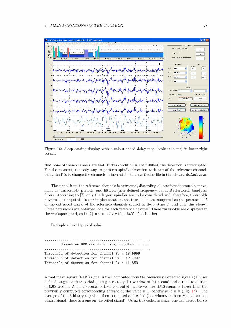
4 MAIN FUNCTIONS OF THE TOOLBOX 28
Figure 16: Sleep scoring display with a colour-coded delay map (scale is in ms) in lower rightcorner.
that none of these channels are bad. If this condition is not fulfilled, the detection is interrupted.For the moment, the only way to perform spindle detection with one of the reference channelsbeing ‘bad’ is to change the channels of interest for that particular file in the file crc defaults.m.
The signal from the reference channels is extracted, discarding all artefacted/arousals, move-ment or ‘unscorable’ periods, and filtered (user-defined frequency band, Butterworth bandpassfilter). According to [?], only the largest spindles are to be considered and, therefore, thresholdshave to be computed. In our implementation, the thresholds are computed as the percentile 95of the extracted signal of the reference channels scored as sleep stage 2 (and only this stage).Three thresholds are obtained, one for each reference channel. These thresholds are displayed inthe workspace, and, as in [?], are usually within 5µV of each other.
Example of workspace display:
....................................................
....... Computing RMS and detecting spindles .......
....................................................
Threshold of detection for channel Fz : 13.9959
Threshold of detection for channel Cz : 12.7297
Threshold of detection for channel Pz : 11.859
A root mean square (RMS) signal is then computed from the previously extracted signals (all userdefined stages or time period), using a rectangular window of 0.1 second and a time resolutionof 0.05 second. A binary signal is then computed: whenever the RMS signal is larger than thepreviously computed corresponding threshold, the value is 1, otherwise it is 0 (Fig. 17). Theaverage of the 3 binary signals is then computed and ceiled (i.e. whenever there was a 1 on onebinary signal, there is a one on the ceiled signal). Using this ceiled average, one can detect bursts
4 MAIN FUNCTIONS OF THE TOOLBOX 29
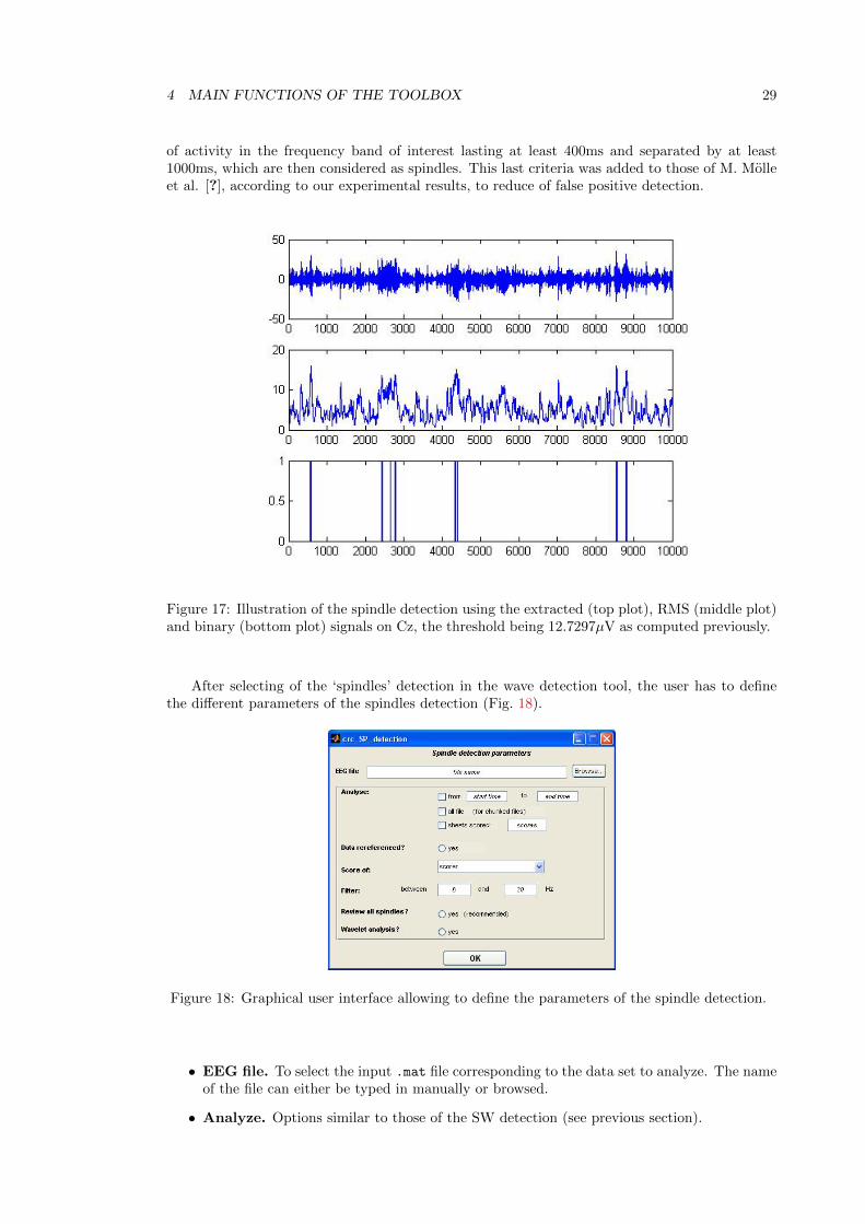
of activity in the frequency band of interest lasting at least 400ms and separated by at least1000ms, which are then considered as spindles. This last criteria was added to those of M. Molleet al. [?], according to our experimental results, to reduce of false positive detection.
Figure 17: Illustration of the spindle detection using the extracted (top plot), RMS (middle plot)and binary (bottom plot) signals on Cz, the threshold being 12.7297µV as computed previously.
After selecting of the ‘spindles’ detection in the wave detection tool, the user has to definethe different parameters of the spindles detection (Fig. 18).
Figure 18: Graphical user interface allowing to define the parameters of the spindle detection.
• EEG file. To select the input .mat file corresponding to the data set to analyze. The nameof the file can either be typed in manually or browsed.
• Analyze. Options similar to those of the SW detection (see previous section).

4 MAIN FUNCTIONS OF THE TOOLBOX 30
• Data rereferenced? To check if the file was already rereferenced.
• Score of. To choose the scorer. Please note that this step determines the time periods usedsince artefacts, arousals, movement or unscorable periods will be withdrawn from furtheranalysis.
• Filter. Choose the filter to apply. Different tests on data sets showed that the 8-20 bandwas optimal for spindles detection. Therefore, if you want to reduce that band (for exampleto 12-15 Hz), please note that filter ripples can affect the signal.
• Review all spindles? Check if you want to review the spindles after detection. Thisoption launches the main display after the detection. After choosing the channels to display(reference channels are preselected), go to the ‘Events’ panel and choose to display ‘SP’types (‘Ant SP’ or ‘Post SP’ if the next option is selected) and ‘All’ values to review thedetected spindles (Fig. 19). Please note that some spindles are not visible when Slow Waveactivity is displayed simultaneously. Therefore, changing the filters might be useful (onepossibility might be to choose the frequency band used to detect the spindles).
Figure 19: Review of detected spindles (here anterior spindles) on the reference channels.
• Wavelet analysis? This option performs a wavelet analysis of the detected spindles (previ-ously epoched around their starting time). The power spectra on the anterior and posteriorchannels in the band 11-16Hz are then compared and the spindle is then labeled as ‘an-terior’ (Ant-SP) or ‘posterior’ (Post-SP) according to the largest power spectrum. Theanterior or posterior character of the channels is computed according to their y-coordinate,the reference being Cz (theoretical 2D coordinates: [0.5 0.5]). Therefore, using theoretical2D coordinates (crc electrodes) or preparing the file using SPM8 can lead to slightlydifferent results as different electrodes could be picked as references.
During detection, different characteristics of the spindles are computed, such as their start-ing and ending points, their duration, the maximum amplitude and the channel on which itoccurred. When the wavelet analysis is selected, the ‘anterior’ or ‘posterior’ character of the spin-dles is also computed, as well as their frequency. All these parameters are saved in the data set

5 ADVANCED USERS 31
(D.CRC.spindles) and spindles are considered as events (to epoch the spindles if needed, codes777 for ‘SP’, 555 for ‘Ant-SP’ and 666 for ‘Post-SP’), which can therefore be marked as ‘good’ or‘bad’ during reviewing.
5 Advanced Users
The first part of this section describes the fields added by FASST to the standard SPM8 struc-ture/object (.mat file). These additional fields do NOT interfere with SPM8 machinery, theymerely contain extra-information used by FASST for the time-frequency analysis, sleep scoringand wave detection. The second part is dedicated to the functions not accessible from the mainGUI.
5.1 Addition to the SPM8 structure
As stated previously FASST does not modify the main fields of the SPM8 structure, except whenevents are added, and all additional structures are placed in seperate subfields (info and CRC atthe moment).
5.1.1 The D.info field
When FASST creates a .mat header from a .vhdr one (BrainProducts Recording System), the timeand the date at the beginning of the recording are stored respectively in the D.info.hour andD.info.date fields. Note that when these informations are available, the time axis of the differentdisplay (scoring, display, frequency representation) is expressed in “clock time”, otherwise it isexpressed in “relative time” from the beginning of the recording.
5.1.2 The D.CRC field
Spectrogram information When the spectrogram of a file is computed, several bits of infor-mation are added to the structure C.CRC.spectpwr:
• .frqname contains the file name of the spectrogram data;
• .frqNsamples is the number of instantaneous power spectra computed for each channel;
• .frqNbins is the number of frequency bins for the spectrogram;
• .frqdata is the file array pointing to the spectrogram data, use it as a matrix;
• .frqscale is the scale factor for each channel;
• .frqbins contains frqNbins elements which are the centre of the frequency bins in Hz;
• .step is the step (in seconds) between two window used to compute two following powerspectra;
• .duration is the length (in seconds) of the windows used to compute the power spectra;
• .frq POI contains the time (in seconds) of the user-defined ‘Periods of Interest’.

5 ADVANCED USERS 32
Scoring information When a file has been scored at least one time, a cell array D.CRC.score
of dimension 8×N is added to the structure, where N is the number of scorer(s). Each columncontains the details of one score, from row one to seven:
• a 1×R vector containing numbers representing the score, where R is the number of scoringwindows. “Stage” labels are defined in the crc defaults.m file. By default they are set as:0 correspond to “Wakefulness”, 1-4 to “Sleep stage 1-4” respectively, 5 to “REM sleep”, 6to “Movement Time”, and 7 to “Unscorable”;
• the name of the scorer;
• the length of a scoring window (in seconds);
• two numbers indicating the time when the light was shut off and door was closed (FPL,first number), and when the light was turned on and the door was opened (OPL, secondnumber). These measures are given in seconds relative to the beginning of the file;
• a T × 2 array, where T is the number of artefact episodes marked. The first column is thebeginning of each artefactual episode and the second, the end of it. All the times expressedin seconds relative to the beginning of the file;
• same as artefact episodes but for arousals;
• same as artefact episodes but for events/episodes of interest;
• a T ×1 cell array, containing the label of each artefact. The labels for ’unspecified’ artefactsare left empty.
SW detection information Other fields added to the D.CRC.SW object for the SW detection:
• .SW, a 1 × T structure array, T being the number of detected waves, containing all theproperties of the waves (type help crc sws detect for the specification of these fields);
• .origin count, a Nel×3 cell array, Nel being the number of non bad EEG electrodes in thefile. This array contains, for each electrode (column 1), the number of waves first detectedon that electrode (column 2) and the total number of waves detected on this electrode(column 3).
Spindle detection information Other fields added to the D.CRC.spindles object for the SPdetection:
• D.spindles contains different properties of the spindles, each in the Nsp×k size, Nsp beingthe number of detected spindles and k depending of the subfield. All fields are explicit,except maxelectrodes, which contains the electrode on which the spindle has maximumamplitude.
Other information Other fields added to the D.CRC structure for display management:
• .lastdisp, time in seconds saving the position when clicking on the ’save position’ button;
• .goodevents, a 1 × Nev vector of binary elements, Nev being the number of events inthe file, as in the D.events field. 1 represents events marked as good (default) while 0represents events marked as ‘bad’ via the display.

6 ACKNOWLEDGMENTS 33
5.2 “Hidden” functions
crc statgen can only be used on files which were previously sleep-scored and computes statisticssuch as the percentage of the different sleep stages, the latency of the sleep stages, the efficiencyof sleep, the total sleep time, the number of arousal per hour, etc. The function creates a textfile, named Statgen.txt, with these values and also return a matrix in the Matlab workspace.The content of this file can be copy-pasted in a cell-formated program such as Excel. If morethan one file is selected, then the text file and the matrix will contains as many lines as there areselected files.
6 Acknowledgments
This M/EEG toolbox is developed with the financial support of the Fonds de la RechercheScientifique-FNRS, the Queen Elizabeth fund, and the University of Liege.
The authors would like to thank the CRC staff for their comments and suggestion during thedevelopment of FASST. A special thank goes to Virginie Sterpenich and Christina Schmidt whosesuggestions were very helpful during the design and the very birth of FASST, and also to PierreMaquet who imagined FASST before we made it real. We are also grateful to all the users atthe CRC (especially Luca Matarazzo, Ariane Foret, Laura Mascetti and Thanh Dang Vu) whohelped us debug the code by boldly using the alpha version of the toolbox. Thanks also go to the“foreign labs” who provided some data sets to test the reading functions and the MR-artefactrejection tools.
References
[1] Philip J. Allen, Oliver Josephs, and Robert Turner. A method for removing imaging artifactfrom continuous EEG recorded during functional MRI. NeuroImage, 12:230–239, 2000.
[2] Stefan Debener, Karen J Mullinger, Rami K Niazy, and Richard W Bowtell. Propertiesof the ballistocardiogram artefact as revealed by EEG recordings at 1.5, 3 and 7 T staticmagnetic field strength. Int J Psychophysiol, 67(3):189–199, March 2008.
[3] Arnaud Delorme and Scott Makeig. EEGLAB: an open source toolbox for analysis of single-trial EEG dynamics. Journal of Neuroscience Methods, 134:9–21, 2004.
[4] Arnaud Delorme, Tim Mullen, Christian Kothe, Zeynep Akalin Acar, Nima Bigdely-Shamlo,Andrey Vankov, and Scott Makeig. EEGLAB, SIFT, NFT, BCILAB, and ERICA: New Toolsfor Advanced EEG Processing. Computational Intelligence and Neuroscience, 2011:12, 2011.
[5] Volkmar Glauche. MATLAB batch system. http://sourceforge.net/projects/matlabbatch/.
[6] G. D. Iannetti, R. K. Niazy, R. G. Wise, P. Jezzard, J. C W Brooks, L. Zambreanu, W. Ven-nart, P. M. Matthews, and I. Tracey. Simultaneous recording of laser-evoked brain potentialsand continuous, high-field functional magnetic resonance imaging in humans. NeuroImage,28(3):708–719, Nov 2005.
[7] B. Kemp, A. Varri, A. C. Rosa, K. D. Nielsen, and J. Gade. A simple format for exchange ofdigitized polygraphic recordings. Electroencephalogr Clin Neurophysiol, 82(5):391–393, May1992.

REFERENCES 34
[8] Bob Kemp. European Data Format. http://www.edfplus.info/.
[9] Bob Kemp and Jesus Olivan. European data format ‘plus’ (EDF+), an EDF alike standardformat for the exchange of physiological data. Clin Neurophysiol, 114(9):1755–1761, 2003.
[10] Yves Leclercq, Evelyne Balteau, Thanh Dang-Vu, Manuel Schabus, Andre Luxen, PierreMaquet, and Christophe Phillips. Rejection of pulse related artefact (PRA) from continuouselectroencephalographic (EEG) time series recorded during functional magnetic resonanceimaging (fMRI) using constraint independent component analysis (cICA). NeuroImage,44(3):679–691, 2009.
[11] Yves Leclercq, Pierre Maquet, Quentin Noirhomme, Christian Degueldre, Eve-lyne Balteau, Andrea Soddu, Jessica Schrouff, Mohamed Bahri, and ChristophePhillips. fMRI Artefact rejection and Sleep Scoring Toolbox (FASST).http://www.montefiore.ulg.ac.be/˜phillips/FASST.html, 2009. Cyclotron Research Centre,University of Liege, Belgium.
[12] Yves Leclercq, Jessica Schrouff, Quentin Noirhomme, Pierre Maquet, and ChristophePhillips. fMRI Artefact rejection and Sleep Scoring Toolbox. Computational Intelligenceand Neuroscience, 2011:11, 2011.
[13] Vladimir Litvak, Jeremie Mattout, Stefan Kiebel, Christophe Phillips, Richard Henson,James Kilner, Gareth Barnes, Robert Oostenveld, Jean Daunizeau, Guillaume Flandin, WillPenny, and Karl Friston. EEG and MEG data analysis in SPM8. Computational Intelligenceand Neuroscience, 2011:32, 2011.
[14] Marcello Massimini, Reto Huber, Fabio Ferrarelli, Sean Hill, and Giulio Tononi. The sleepslow oscillation as a traveling wave. J Neurosci, 24(31):6862–6870, Aug 2004.
[15] Members and collaborators of the Wellcome Trust Centre for Neuroimaging. Statistical Para-metric Mapping, SPM8. http://www.fil.ion.ucl.ac.uk/spm, 2008. Wellcome Trust Centre forNeuroimaging, University College London, UK.
[16] Matthias Molle, Lisa Marshall, Steffen Gais, and Jan Born. Grouping of spindle activityduring slow oscillations in human non-rapid eye movement sleep. J Neurosci, 22(24):10941–10947, Dec 2002.
[17] R. K. Niazy, C. F. Beckmann, G. D. Iannetti, J. M. Brady, and S. M. Smith. Removal of fMRIenvironment artifacts from EEG data using optimal basis sets. NeuroImage, 28(3):720–737,Nov 2005.
[18] Rami K. Niazy. FMRIB plug-in for EEGLAB. http://users.fmrib.ox.ac.uk/˜rami/fmribplugin/,2006. Centre for Functional MRI of the Brain (FMRIB), University of Oxford, UK.
[19] Robert Oostenveld, Pascal Fries, Eric Maris, and Jan-Mathijs Schoffelen. FieldTrip: Opensource software for advanced analysis of MEG, EEG, and invasive electrophysiological data.Computational Intelligence and Neuroscience, 2011:9, 2011.
[20] Robert Oostenveld, Jan-Mathijs Schoffelen, Eric Maris, Pascal Fries, and Ole Jensen. Field-trip toolbox for EEG/MEG-analysis. http://www.ru.nl/neuroimaging/fieldtrip, 2009. Don-ders Institute for Brain, Cognition and Behaviour, Radboud University Nijmegen, theNetherlands.
[21] Hanchuan Peng, Fuhui Long, and Chris Ding. Feature selection based on mutual information:criteria of max-dependency, max-relevance, and min-redundancy. IEEE Transactions onPattern Analysis and Machine Intelligence, 27(8):1226–1238, 2005.
[22] Christophe Phillips, Gerald Thielen, and Pierre Maquet. Iteratively applied ICA to rejectballistocardiogram artefact of EEG data acquired during sleep fMRI. Abstract of the HumanBrain Mapping conference, June 2006.