fast algorithm for digital signal processing - vlsi signal
TRANSCRIPT
1
VSP Lecture6 - Fast Algorithms for DSP ([email protected]) 3-1
5012: VLSI Signal Processing
5012: VLSI Signal 5012: VLSI Signal ProcessingProcessing
Lecture 6 Fast Algorithms for Digital Lecture 6 Fast Algorithms for Digital Signal ProcessingSignal Processing
VSP Lecture6 - Fast Algorithms for DSP ([email protected]) 3-2
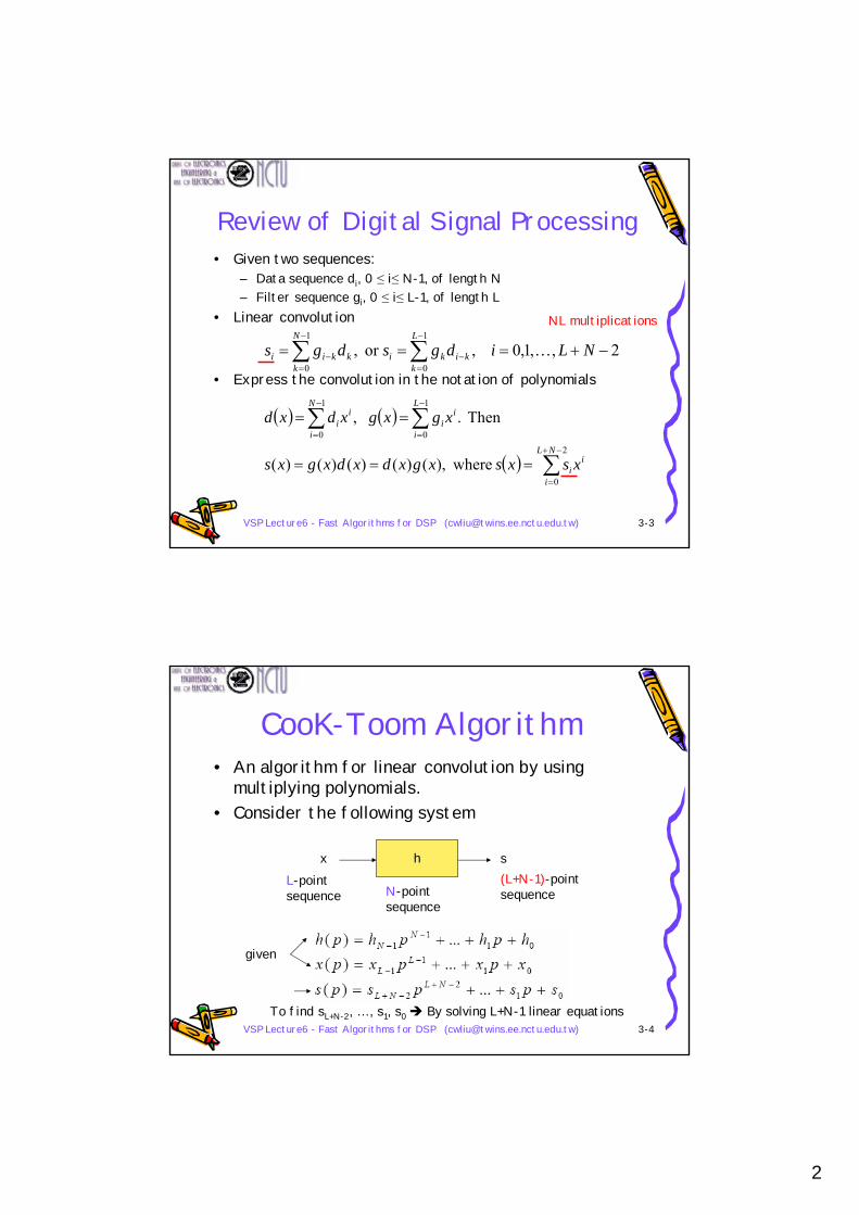
Algorithm Strength Reduction• Motivation
– The number of strong operations, such as multiplications, is reduced possibly at the expense of an increase in the number of weaker operations, such as additions.
• Reduce computation complexity• Example: Complex multiplication
– (a+jb)(c+jd)=e+jf, a,b,c,d,e,f ∈ R– The direct implementation requires 4 multiplications and 2
additions
– However, the number of multiplication can be reduced to 3 at the expense of 3 extra additions by using the identities
⎥⎦
⎤⎢⎣
⎡⎥⎦
⎤⎢⎣
⎡ −=⎥
⎦
⎤⎢⎣
⎡ba
cddc
fe
)()()()(
baddcbbcadbaddcabdac
−++=+−+−=− 3 multiplications
5 additions
2
VSP Lecture6 - Fast Algorithms for DSP ([email protected]) 3-3
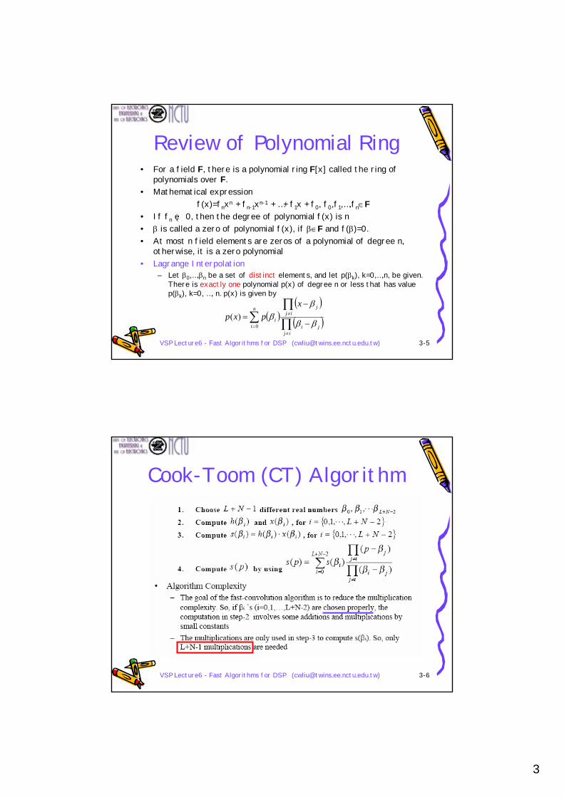
Review of Digital Signal Processing• Given two sequences:
– Data sequence di, 0 ≤ i≤ N-1, of length N– Filter sequence gi, 0 ≤ i≤ L-1, of length L
• Linear convolution
• Express the convolution in the notation of polynomials∑ ∑−
=
−
=−− −+===
1
0
1
0
2,,1,0 ,or ,N
k
L
kkikikkii NLidgsdgs K
( ) ( )
( ) ∑
∑∑−+
=
−
=
−
=
===
==
2
0
1
0
1
0
where),()()()()(
Then . ,
NL
i
ii
L
i
ii
N
i
ii
xsxsxgxdxdxgxs
xgxgxdxd
NL multiplications
VSP Lecture6 - Fast Algorithms for DSP ([email protected]) 3-4
CooK-Toom Algorithm• An algorithm for linear convolution by using
multiplying polynomials.• Consider the following system
hx sL-point sequence N-point
sequence
(L+N-1)-point sequence
given
To find sL+N-2, …, s1, s0 By solving L+N-1 linear equations
3
VSP Lecture6 - Fast Algorithms for DSP ([email protected]) 3-5
Review of Polynomial Ring• For a field F, there is a polynomial ring F[x] called the ring of
polynomials over F.• Mathematical expression
f(x)=fnxn + fn-1xn-1 + …+ f1x + f0, f0,f1,…,fn∈F• If fn≠ 0, then the degree of polynomial f(x) is n• β is called a zero of polynomial f(x), if β∈F and f(β)=0.• At most n field elements are zeros of a polynomial of degree n,
otherwise, it is a zero polynomial• Lagrange Interpolation
– Let β0,…,βn be a set of distinct elements, and let p(βk), k=0,…,n, be given. There is exactly one polynomial p(x) of degree n or less that has value p(βk), k=0, …, n. p(x) is given by
( )( )( )∏
∏∑
≠
≠
= −
−=
ijji
ijjn
ii
xpxp
ββ
ββ
0)(
VSP Lecture6 - Fast Algorithms for DSP ([email protected]) 3-6
Cook-Toom (CT) Algorithm
4
VSP Lecture6 - Fast Algorithms for DSP ([email protected]) 3-7
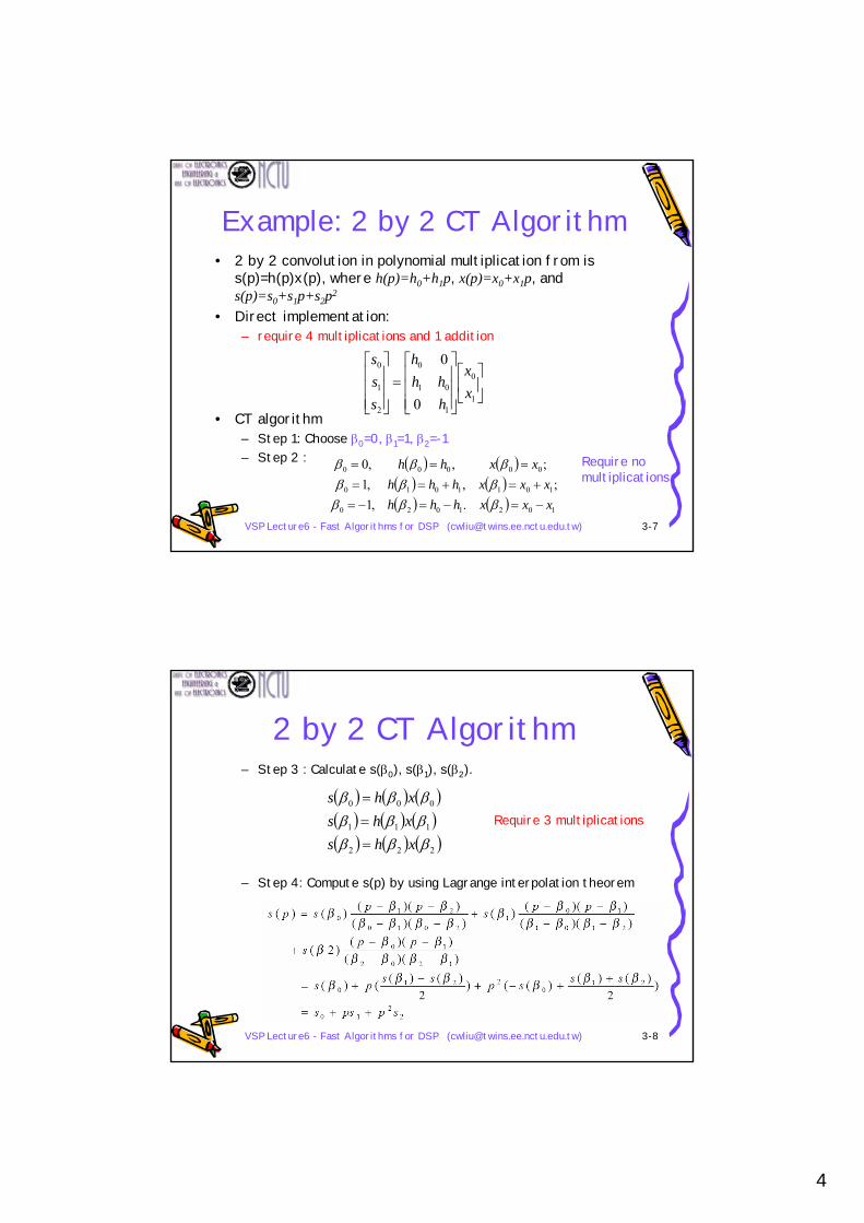
Example: 2 by 2 CT Algorithm• 2 by 2 convolution in polynomial multiplication from is
s(p)=h(p)x(p), where h(p)=h0+h1p, x(p)=x0+x1p, and s(p)=s0+s1p+s2p2
• Direct implementation: – require 4 multiplications and 1 addition
• CT algorithm – Step 1: Choose β0=0, β1=1, β2=-1– Step 2 :
⎥⎦
⎤⎢⎣
⎡
⎥⎥⎥
⎦
⎤
⎢⎢⎢
⎣
⎡=
⎥⎥⎥
⎦
⎤
⎢⎢⎢
⎣
⎡
1
0
1
01
0
2
1
0
0
0
xx
hhh
h
sss
Require no multiplications
( ) ( )( ) ( )( ) ( ) 1021020
1011010
00000
.,1;,,1
;,,0
xxxhhhxxxhhh
xxhh
−=−=−=+=+==
===
βββββββββ
VSP Lecture6 - Fast Algorithms for DSP ([email protected]) 3-8
2 by 2 CT Algorithm– Step 3 : Calculate s(β0), s(β1), s(β2).
– Step 4: Compute s(p) by using Lagrange interpolation theorem
( ) ( ) ( )( ) ( ) ( )( ) ( ) ( )222
111
000
βββββββββ
xhsxhsxhs
===
Require 3 multiplications
5
VSP Lecture6 - Fast Algorithms for DSP ([email protected]) 3-9
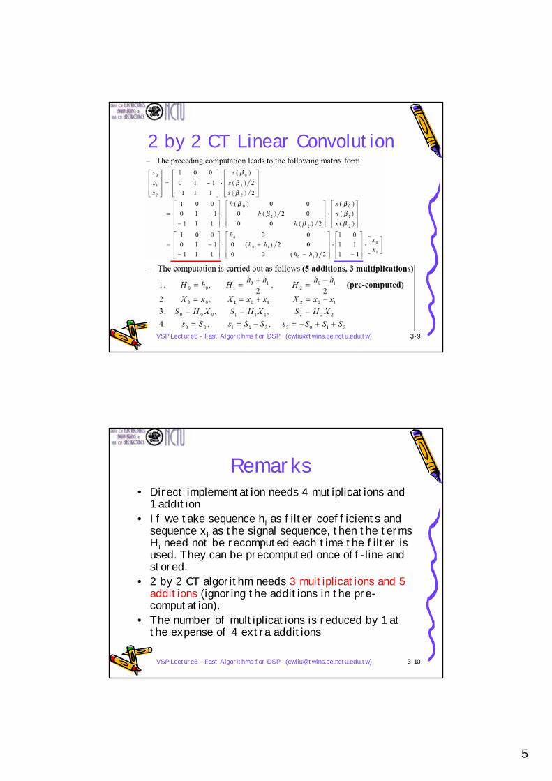
2 by 2 CT Linear Convolution
VSP Lecture6 - Fast Algorithms for DSP ([email protected]) 3-10
Remarks• Direct implementation needs 4 mutiplications and
1 addition• If we take sequence hi as filter coefficients and
sequence xi as the signal sequence, then the terms Hi need not be recomputed each time the filter is used. They can be precomputed once off-line and stored.
• 2 by 2 CT algorithm needs 3 multiplications and 5 additions (ignoring the additions in the pre-computation).
• The number of multiplications is reduced by 1 at the expense of 4 extra additions
6
VSP Lecture6 - Fast Algorithms for DSP ([email protected]) 3-11
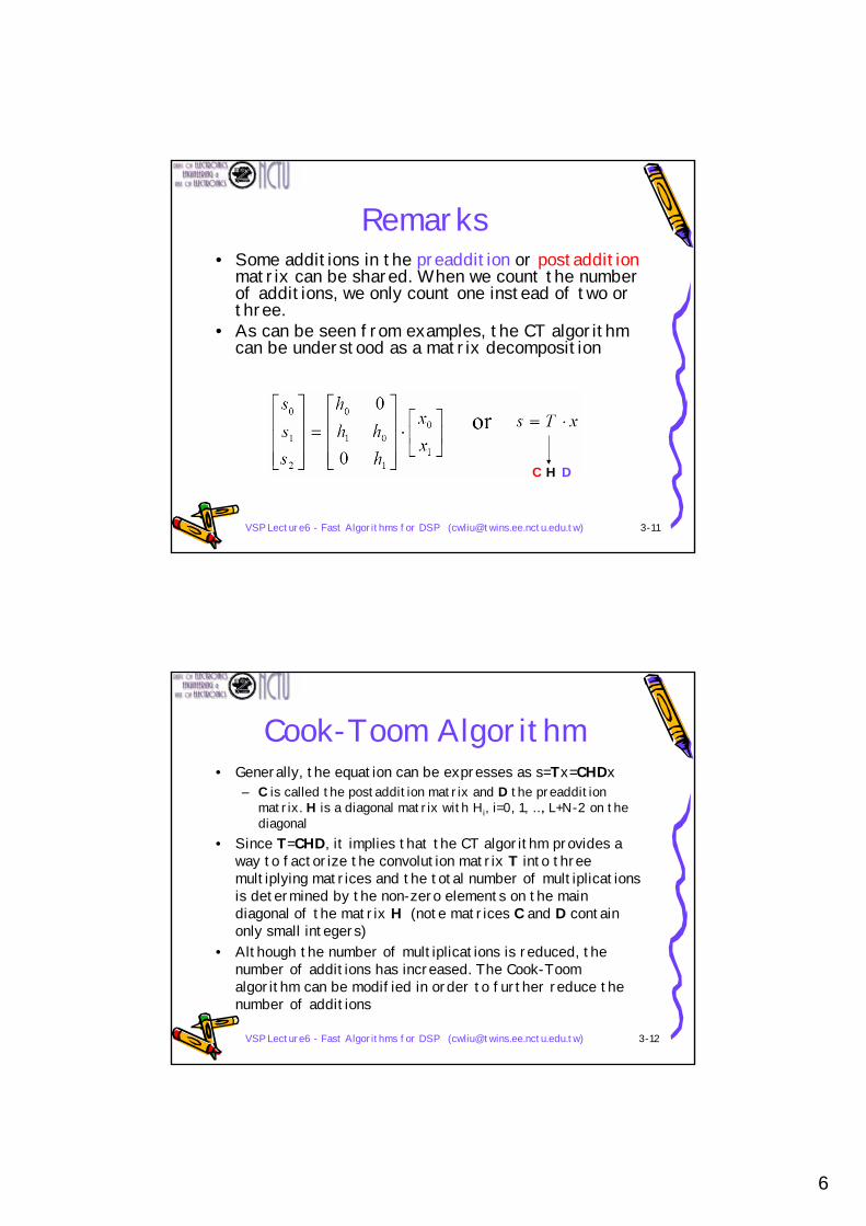
Remarks• Some additions in the preaddition or postaddition
matrix can be shared. When we count the number of additions, we only count one instead of two or three.
• As can be seen from examples, the CT algorithm can be understood as a matrix decomposition
C H D
VSP Lecture6 - Fast Algorithms for DSP ([email protected]) 3-12
Cook-Toom Algorithm• Generally, the equation can be expresses as s=Tx=CHDx
– C is called the postaddition matrix and D the preadditionmatrix. H is a diagonal matrix with Hi, i=0, 1, …, L+N-2 on the diagonal
• Since T=CHD, it implies that the CT algorithm provides a way to factorize the convolution matrix T into three multiplying matrices and the total number of multiplications is determined by the non-zero elements on the main diagonal of the matrix H (note matrices C and D contain only small integers)
• Although the number of multiplications is reduced, the number of additions has increased. The Cook-Toomalgorithm can be modified in order to further reduce the number of additions
7
VSP Lecture6 - Fast Algorithms for DSP ([email protected]) 3-13
Concluding Remarks• The Cook-Toom algorithm is efficient as
measured by the number of multiplications• As the size of the problem increases, the number
of additions increase rapidly• The choices of βi=0, ±1 are good, while the choices
of ±2, ±4 (or other small integers) result in complicated pre-addition and post-addition matrices.
• For larger problems, CT algorithm becomes cumbersome
• Winograd Algorithm
VSP Lecture6 - Fast Algorithms for DSP ([email protected]) 3-14
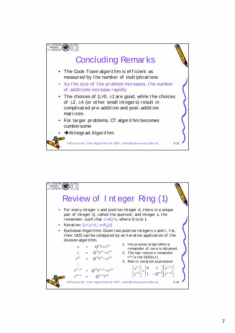
Review of Integer Ring (1)• For every integer c and positive integer d, there is a unique
pair of integer Q, called the quotient, and integer s, the remainder, such that c=dQ+s, where 0≤s≤d-1
• Notation: Q=⎣c/d⎦, s=Rd[c]• Euclidean Algorithm: Given two positive integers s and t, t<s,
their GCD can be computed by an iterative application of the division algorithm.
)()1()1(
)()1()()2(
)3()2()3()1(
)2()1()2(
)1()1(
nnn
nnnn
tQtttQt
ttQtttQt
ttQs
−−
−−
=+=
+=+=+=
M
1. the process stops when a remainder of zero is obtained.
2. The last nonzero remainder t(n) is the GCD(s,t)
3. Matrix notation expression
⎥⎦
⎤⎢⎣
⎡⎥⎦
⎤⎢⎣
⎡−
=⎥⎦
⎤⎢⎣
⎡−
−
)1(
)1(
)()(
)(
110
r
r
rr
r
ts
Qts
8
VSP Lecture6 - Fast Algorithms for DSP ([email protected]) 3-15
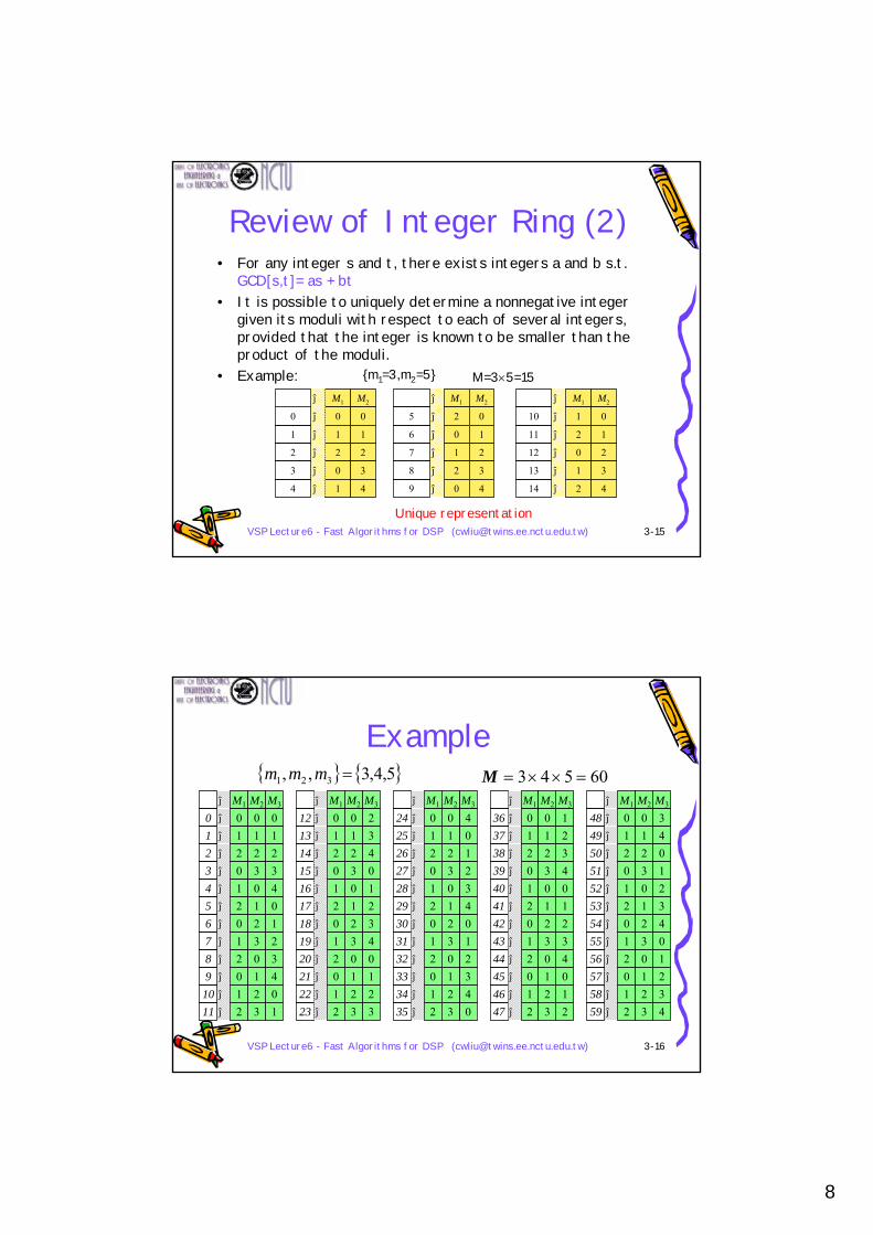
Review of Integer Ring (2)• For any integer s and t, there exists integers a and b s.t.
GCD[s,t]= as + bt• It is possible to uniquely determine a nonnegative integer
given its moduli with respect to each of several integers, provided that the integer is known to be smaller than the product of the moduli.
• Example:M1
0
1
2
0
1
M2
0
1
2
3
4
→
→
→
→
→
→
→
→
→
→
→
→
→
→
→
→
→
→M1
2
0
1
2
0
M2
0
1
2
3
4
M1
1
2
0
1
2
M2
0
1
2
3
4
0
1
2
3
4
5
6
7
8
9
10
11
12
13
14
{m1=3,m2=5} M=3×5=15
Unique representation
VSP Lecture6 - Fast Algorithms for DSP ([email protected]) 3-16
4567891011
0123
→
→
→
→
→
→
→
→
→
→
→
→
→
M1
012012012012
M2
012301230123
M3
012340123401
1617181920212223
12131415
→
→
→
→
→
→
→
→
→
→
→
→
→
M3
234012340123
2829303132333435
24252627
→
→
→
→
→
→
→
→
→
→
→
→
→
M3
401234012340
4041424344454647
36373839
→
→
→
→
→
→
→
→
→
→
→
→
→
M3
123401234012
5253545556575859
48495051
→
→
→
→
→
→
→
→
→
→
→
→
→
M3
340123401234
M1
012012012012
M1
012012012012
M1
012012012012
M1
012012012012
M2
012301230123
M2
012301230123
M2
012301230123
M2
012301230123
{ } { }5,4,3,, 321 =mmm 60543 =××=M
Example
9
VSP Lecture6 - Fast Algorithms for DSP ([email protected]) 3-17
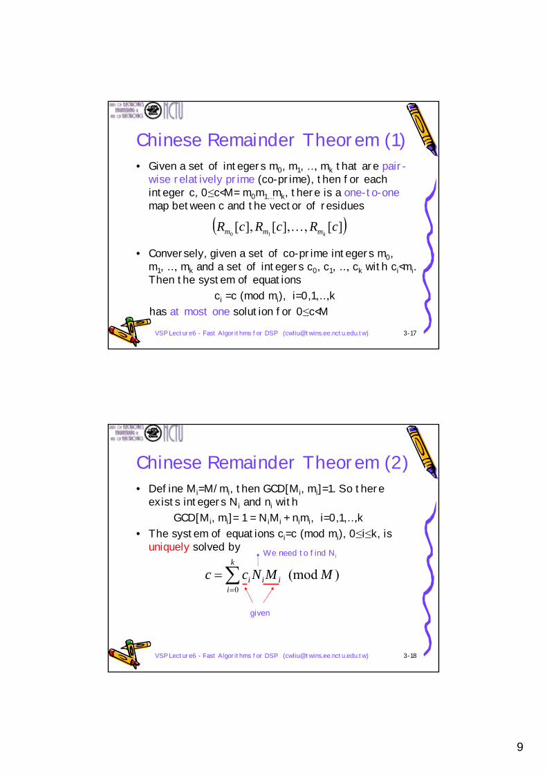
Chinese Remainder Theorem (1)• Given a set of integers m0, m1, …, mk that are pair-
wise relatively prime (co-prime), then for each integer c, 0≤c<M= m0m1…mk, there is a one-to-onemap between c and the vector of residues
• Conversely, given a set of co-prime integers m0, m1, …, mk and a set of integers c0, c1, …, ck with ci<mi. Then the system of equations
ci =c (mod mi), i=0,1,…,khas at most one solution for 0≤c<M
( )][,],[],[10
cRcRcRkmmm K
VSP Lecture6 - Fast Algorithms for DSP ([email protected]) 3-18
Chinese Remainder Theorem (2)• Define Mi=M/mi, then GCD[Mi, mi]=1. So there
exists integers Ni and ni with GCD[Mi, mi]= 1 = NiMi + nimi, i=0,1,…,k
• The system of equations ci=c (mod mi), 0≤i≤k, is uniquely solved by
∑=
=k
iiii MMNcc
0) (mod
given
We need to find Ni

10
VSP Lecture6 - Fast Algorithms for DSP ([email protected]) 3-19
GCD Example• GCD(993,186)
993 186 993=5×186+63930
63 186=2×63+60
63=1×60+3
12660
603 60=20×3+0
600
( )
( )
( )186169933
1861186599331861633
63218616360163
3186,993
×−×=×−×−×=
×−×=×−×−=
×−==GCD
VSP Lecture6 - Fast Algorithms for DSP ([email protected]) 3-20
Remark1.
2.
) (mod ) (mod
) (mod ) (mod 0
ii
iiii
k
iiiiii
mcmMNc
mMNcmc
==
=∑=
( )iii
iiiiii
mMNmMGCDmnMN
mod 1have then we,1),(
===+

11
VSP Lecture6 - Fast Algorithms for DSP ([email protected]) 3-21
Example• m0=3, m1=4, m2=5. Then by Euclidean theorem, we have
• The integer c can be calculated as
• Example
;15)5(12)2(,12,5;14)4(15)1(,15,4;13)7(20)1(,20,3
02
11
00
=+−===+−===+−==
MmMmMm
Ni
ni
( )
( ) ( )60 mod 241520
mod
210
0
ccc
MMNcck
iiii
−−−=
=∑=
( )17)60 (mod )224115220( ,Conversely
)2,1,2(,, i.e.,17 210
=×−×−×−===
ccccc
VSP Lecture6 - Fast Algorithms for DSP ([email protected]) 3-22
Remarks• By taking residues, large integers are broken
down into small pieces (that may be easy to add and multiply)
• Examples:7→(1, 3, 2 )
+3→(0, 3, 3 )10→(1 mod 3, 6 mod 4, 5 mod 5) = (1,2,0)
7→(1, 3, 2 )×3→(0, 3, 3 )21→(0 mod 3, 9 mod 4, 6 mod 5) = (0,1,1)
12
VSP Lecture6 - Fast Algorithms for DSP ([email protected]) 3-23
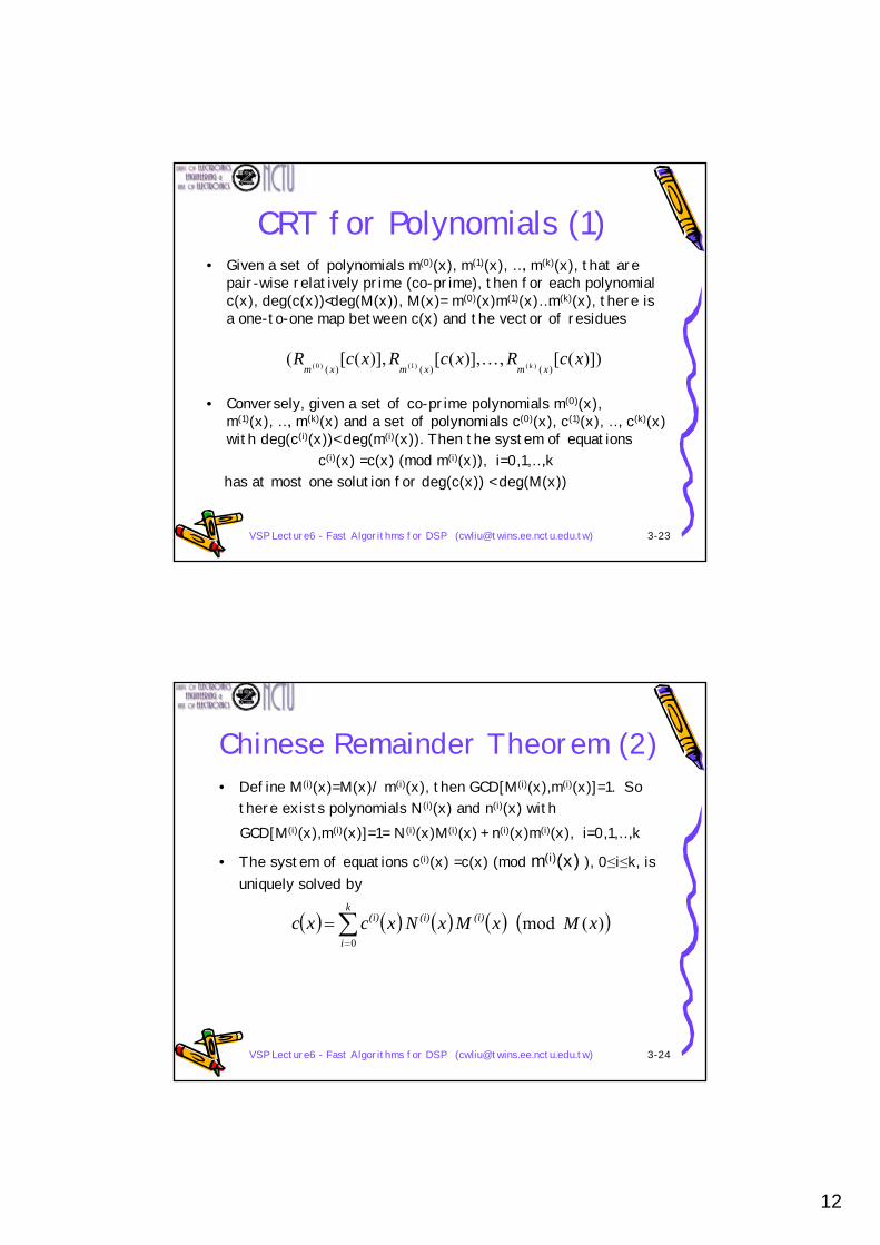
CRT for Polynomials (1)• Given a set of polynomials m(0)(x), m(1)(x), …, m(k)(x), that are
pair-wise relatively prime (co-prime), then for each polynomial c(x), deg(c(x))<deg(M(x)), M(x)= m(0)(x)m(1)(x)…m(k)(x), there is a one-to-one map between c(x) and the vector of residues
• Conversely, given a set of co-prime polynomials m(0)(x), m(1)(x), …, m(k)(x) and a set of polynomials c(0)(x), c(1)(x), …, c(k)(x) with deg(c(i)(x))< deg(m(i)(x)). Then the system of equations
c(i)(x) =c(x) (mod m(i)(x)), i=0,1,…,khas at most one solution for deg(c(x)) < deg(M(x))
)])([,)],([)],([()()()( )()1()0( xcRxcRxcR
xmxmxm kK
VSP Lecture6 - Fast Algorithms for DSP ([email protected]) 3-24
Chinese Remainder Theorem (2)• Define M(i)(x)=M(x)/ m(i)(x), then GCD[M(i)(x),m(i)(x)]=1. So
there exists polynomials N(i)(x) and n(i)(x) with GCD[M(i)(x),m(i)(x)]=1= N(i)(x)M(i)(x) + n(i)(x)m(i)(x), i=0,1,…,k
• The system of equations c(i)(x) =c(x) (mod m(i)(x) ), 0≤i≤k, is uniquely solved by
( ) ( ) ( ) ( ) ( )∑=
=k
i
(i)(i)(i) xM xMxNxcxc0
)( mod
13
VSP Lecture6 - Fast Algorithms for DSP ([email protected]) 3-25
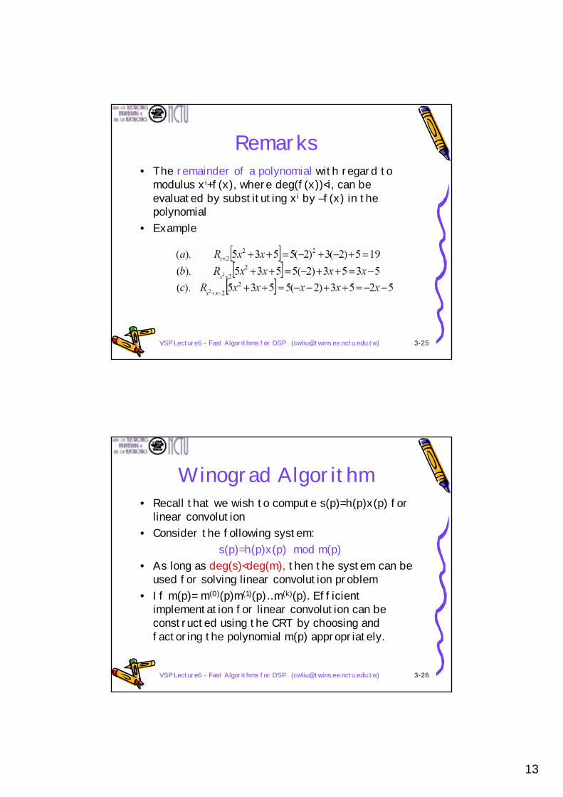
Remarks• The remainder of a polynomial with regard to
modulus xi+f(x), where deg(f(x))<i, can be evaluated by substituting xi by –f(x) in the polynomial
• Example
VSP Lecture6 - Fast Algorithms for DSP ([email protected]) 3-26
Winograd Algorithm• Recall that we wish to compute s(p)=h(p)x(p) for
linear convolution• Consider the following system:
s(p)=h(p)x(p) mod m(p)• As long as deg(s)<deg(m), then the system can be
used for solving linear convolution problem• If m(p)= m(0)(p)m(1)(p)…m(k)(p). Efficient
implementation for linear convolution can be constructed using the CRT by choosing and factoring the polynomial m(p) appropriately.
14
VSP Lecture6 - Fast Algorithms for DSP ([email protected]) 3-27
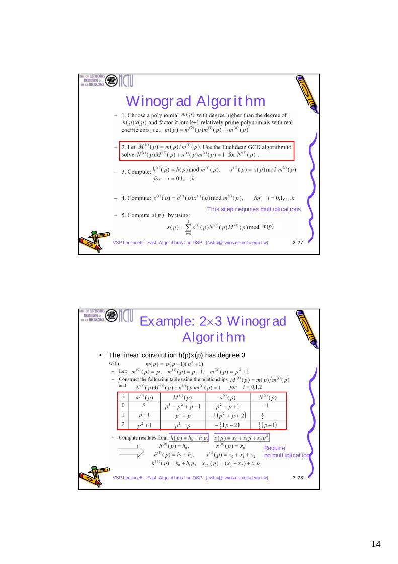
Winograd Algorithm
This step requires multiplications
m(p)
VSP Lecture6 - Fast Algorithms for DSP ([email protected]) 3-28
Example: 2×3 WinogradAlgorithm
• The linear convolution h(p)x(p) has degree 3
Require no multiplication

15
VSP Lecture6 - Fast Algorithms for DSP ([email protected]) 3-29
Example: 2×3 WinogradAlgorithm
Require multiplication
m(p)
VSP Lecture6 - Fast Algorithms for DSP ([email protected]) 3-30
Example: 2×3 WinogradAlgorithm
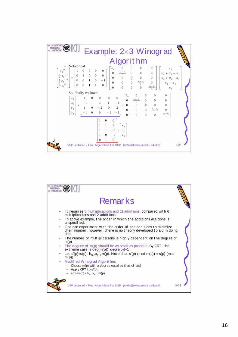
16
VSP Lecture6 - Fast Algorithms for DSP ([email protected]) 3-31
Example: 2×3 WinogradAlgorithm
VSP Lecture6 - Fast Algorithms for DSP ([email protected]) 3-32
Remarks• It requires 5 multiplications and 11 additions, compared with 6
multiplications and 2 additions.• In above example, the order in which the additions are done is
unspecified. • One can experiment with the order of the additions to minimize
their number, however, there is no theory developed to aid in doing this.
• The number of multiplications is highly dependent on the degree of m(p)
• The degree of m(p) should be as small as possible. By CRT, the extreme case is deg(m(p))=deg(s(p))+1
• Let s’(p)=s(p)- hN-1xL-1 m(p). Note that s’(p) (mod m(p)) = s(p) (mod m(p))
• Modified Winograd Algorithm:– Choose m(p) with a degree equal to that of s(p)– Apply CRT to s’(p)– s(p)=s’(p)+ hN-1xL-1 m(p).
17
VSP Lecture6 - Fast Algorithms for DSP ([email protected]) 3-33
Iterated Convolution• To make use of efficient short-length convolution
algorithms iteratively, one can build long convolutions
• These algorithms do not achieve minimal multiplication complexity, but achieve a good balance between multiplications and addition complexity
• Iterated Convolution algorithm– Decompose the long convolution algorithm for short
convolutions– Construct fast convolution algorithm for short
convolutions– Use the short convolution algorithms to iteratively (or
hierarchically) implement the long convolution
VSP Lecture6 - Fast Algorithms for DSP ([email protected]) 3-34
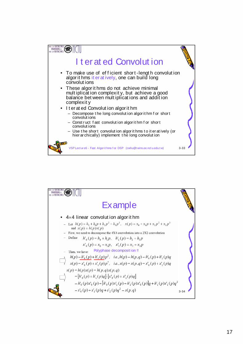
Example• 4×4 linear convolution algorithm
Polyphase decomposition !!
18
VSP Lecture6 - Fast Algorithms for DSP ([email protected]) 3-35
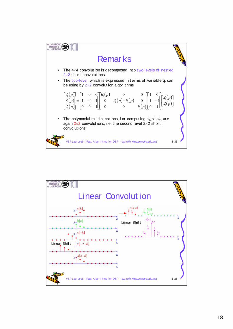
Remarks• The 4×4 convolution is decomposed into two levels of nested
2×2 short convolutions• The top-level, which is expressed in terms of variable q, can
be using by 2×2 convolution algorithms
• The polynomial multiplications, for computing s’0,s’1,s’2, are again 2×2 convolutions, i.e. the second level 2×2 short convolutions
( )( )( )
( )( ) ( )
( )
( )( )⎥⎦
⎤⎢⎣
⎡′′
⎥⎥⎥
⎦
⎤
⎢⎢⎢
⎣
⎡−
⎥⎥⎥
⎦
⎤
⎢⎢⎢
⎣
⎡
′′−′
′
⎥⎥⎥
⎦
⎤
⎢⎢⎢
⎣
⎡−=
⎥⎥⎥
⎦
⎤
⎢⎢⎢
⎣
⎡
′′′
pxpx
phphph
ph
pspsps
1
0
1
10
0
2
1
0
1011
01
000000
100111001
VSP Lecture6 - Fast Algorithms for DSP ([email protected]) 3-36
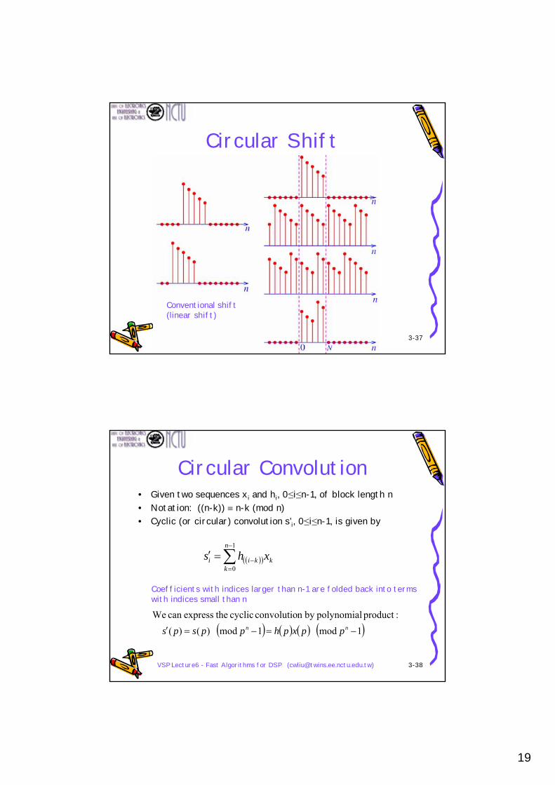
Linear Convolution
Linear Shift
Linear Shift
19
VSP Lecture6 - Fast Algorithms for DSP ([email protected]) 3-37
Circular Shift
Conventional shift(linear shift)
VSP Lecture6 - Fast Algorithms for DSP ([email protected]) 3-38
Circular Convolution• Given two sequences xi and hi, 0≤i≤n-1, of block length n• Notation: ((n-k)) ≡ n-k (mod n)• Cyclic (or circular) convolution s’i, 0≤i≤n-1, is given by
( )( )∑−
=−=′
1
0
n
kkkii xhs
( ) ( ) ( ) ( )1mod 1mod )()( :product polynomialby n convolutio cyclic theexpresscan We
−=−=′ nn ppxphppsps
Coefficients with indices larger than n-1 are folded back into termswith indices small than n
20
VSP Lecture6 - Fast Algorithms for DSP ([email protected]) 3-39
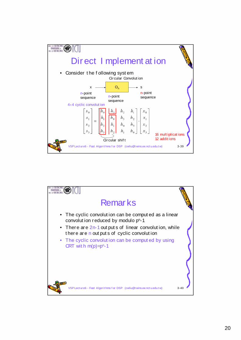
Direct Implementation• Consider the following system
Ohx sn-point sequence n-point
sequence
n-point sequence
4×4 cyclic convolution
16 multiplications12 additions
Circular Convolution
Circular shift
VSP Lecture6 - Fast Algorithms for DSP ([email protected]) 3-40
Remarks• The cyclic convolution can be computed as a linear
convolution reduced by modulo pn-1• There are 2n-1 outputs of linear convolution, while
there are n outputs of cyclic convolution• The cyclic convolution can be computed by using
CRT with m(p)=pn-1
21
VSP Lecture6 - Fast Algorithms for DSP ([email protected]) 3-41
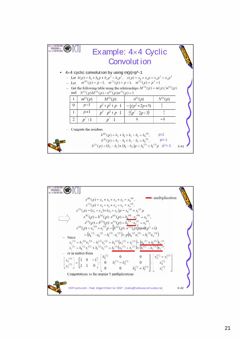
Example: 4×4 Cyclic Convolution
• 4×4 cyclic convolution by using m(p)=p4-1
p=1p=-1
p2=-1
VSP Lecture6 - Fast Algorithms for DSP ([email protected]) 3-42
Example
22
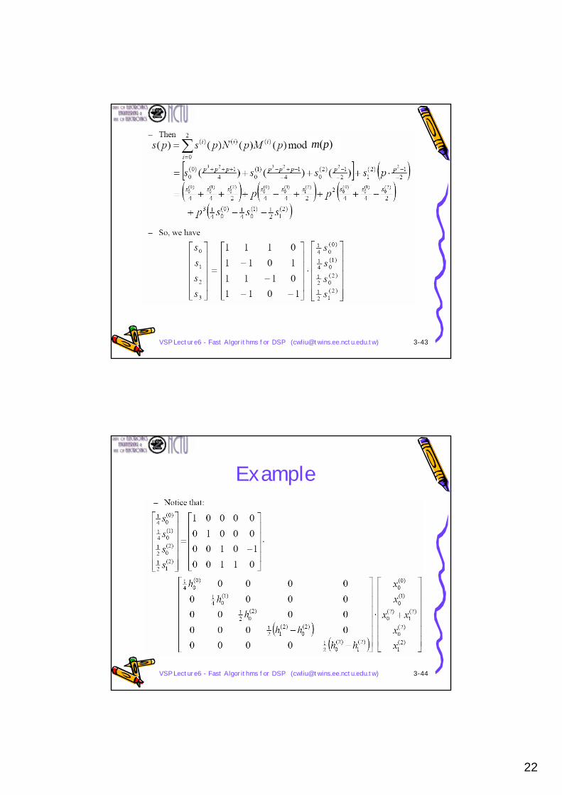
VSP Lecture6 - Fast Algorithms for DSP ([email protected]) 3-43
Examplem(p)
VSP Lecture6 - Fast Algorithms for DSP ([email protected]) 3-44
Example
23
VSP Lecture6 - Fast Algorithms for DSP ([email protected]) 3-45
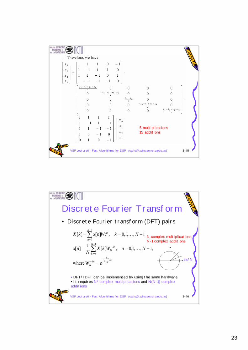
5 multiplications15 additions
VSP Lecture6 - Fast Algorithms for DSP ([email protected]) 3-46
Discrete Fourier Transform• Discrete Fourier transform (DFT) pairs
knN
jknN
N
k
knN
N
n
knN
eW
NnWkXN
nx
NkWnxkX
π2
1
0
1
0
where
,1,,1,0 ,][1][
1,,1,0 ,][][
−−
−
=
−
−
=
=
−==
−==
∑
∑
K
K
• DFT/IDFT can be implemented by using the same hardware• It requires N2 complex multiplications and N(N-1) complex additions
N complex multiplicationsN-1 complex additions
2π/N
24
VSP Lecture6 - Fast Algorithms for DSP ([email protected]) 3-47
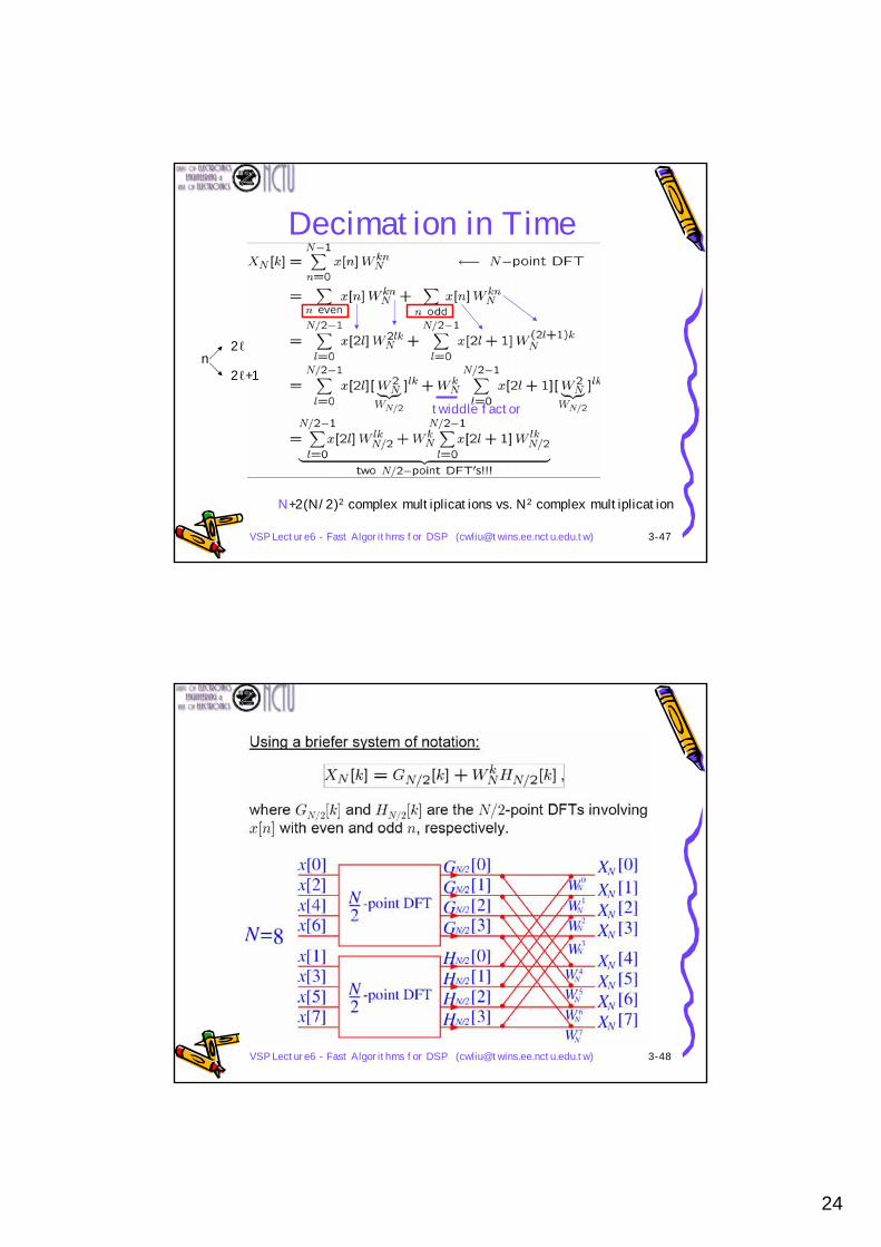
Decimation in Time
N+2(N/2)2 complex multiplications vs. N2 complex multiplication
twiddle factor
n2ℓ
2ℓ+1
VSP Lecture6 - Fast Algorithms for DSP ([email protected]) 3-48
25
VSP Lecture6 - Fast Algorithms for DSP ([email protected]) 3-49
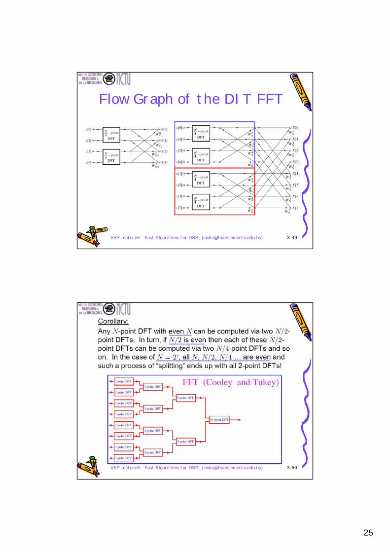
Flow Graph of the DIT FFT
VSP Lecture6 - Fast Algorithms for DSP ([email protected]) 3-50
26
VSP Lecture6 - Fast Algorithms for DSP ([email protected]) 3-51
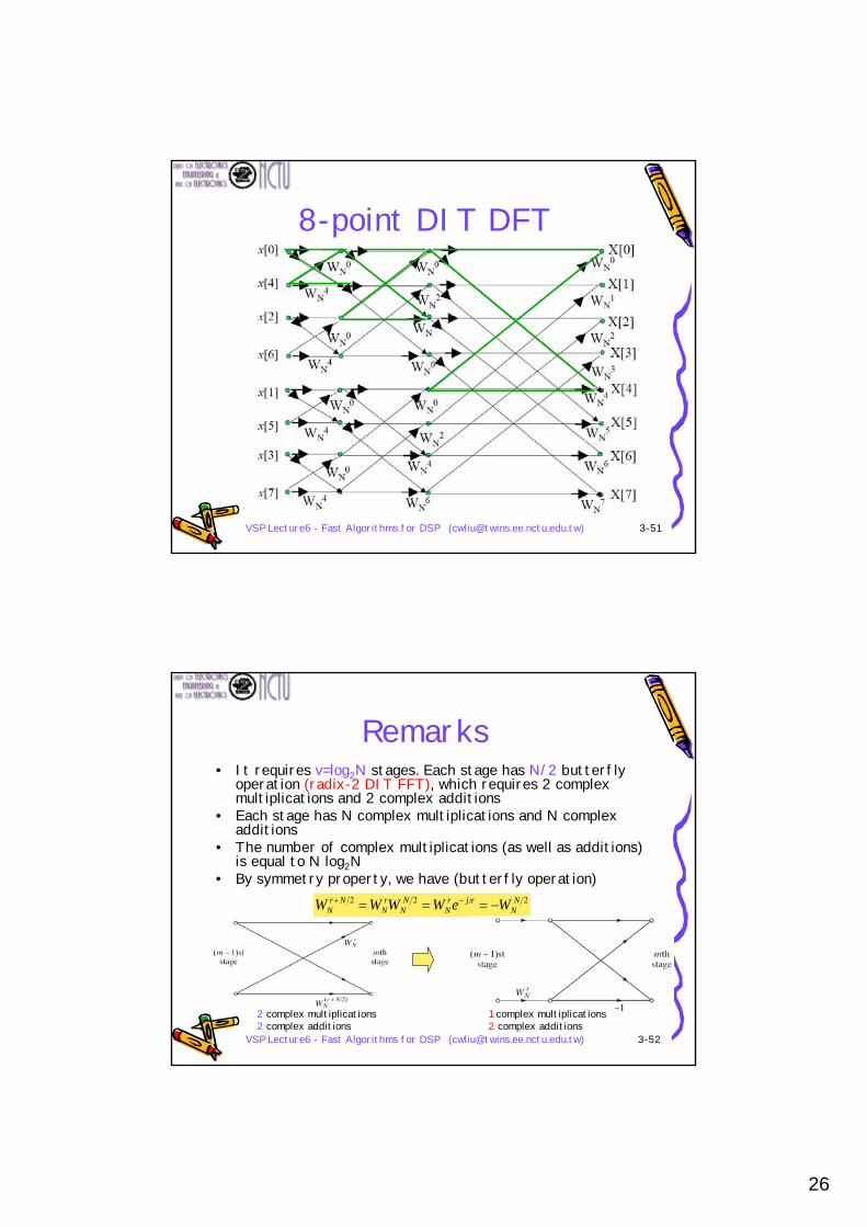
8-point DIT DFT
VSP Lecture6 - Fast Algorithms for DSP ([email protected]) 3-52
Remarks• It requires v=log2N stages. Each stage has N/2 butterfly
operation (radix-2 DIT FFT), which requires 2 complex multiplications and 2 complex additions
• Each stage has N complex multiplications and N complex additions
• The number of complex multiplications (as well as additions) is equal to N log2N
• By symmetry property, we have (butterfly operation)222 N
Njr
NN
Nr
NNr
N WeWWWW −=== −+ π
2 complex multiplications2 complex additions
1 complex multiplications2 complex additions
27
VSP Lecture6 - Fast Algorithms for DSP ([email protected]) 3-53
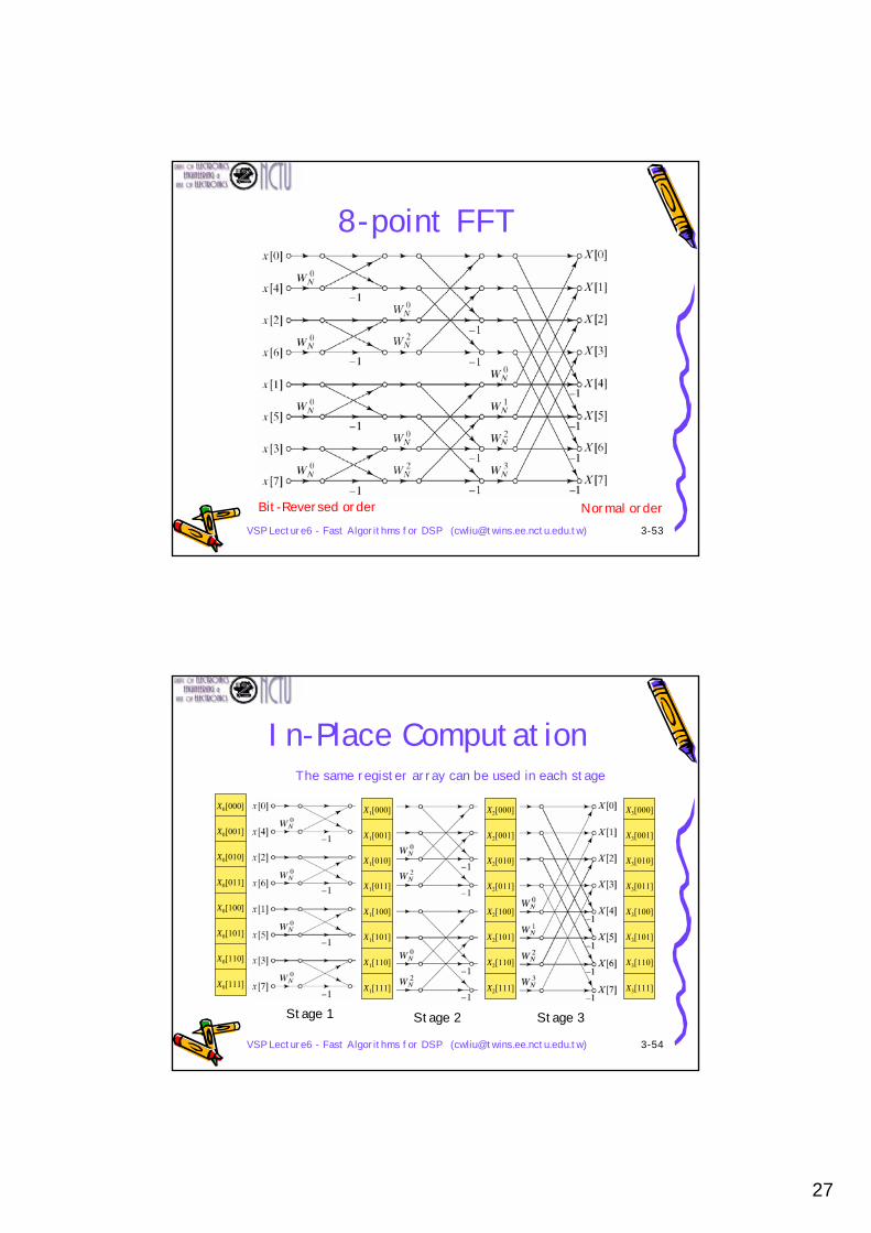
8-point FFT
Normal orderBit-Reversed order
VSP Lecture6 - Fast Algorithms for DSP ([email protected]) 3-54
In-Place Computation
Stage 1
X0[000]
X0[001]
X0[010]
X0[011]
X0[100]
X0[101]
X0[110]
X0[111]
X1[000]
X1[001]
X1[010]
X1[011]
X1[100]
X1[101]
X1[110]
X1[111]
X2[000]
X2[001]
X2[010]
X2[011]
X2[100]
X2[101]
X2[110]
X2[111]
Stage 3Stage 2
X3[000]
X3[001]
X3[010]
X3[011]
X3[100]
X3[101]
X3[110]
X3[111]
The same register array can be used in each stage
28
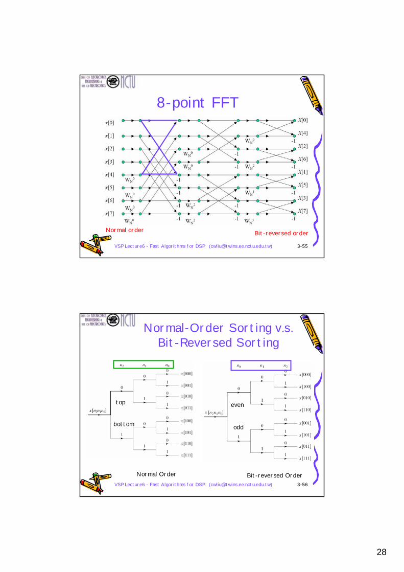
VSP Lecture6 - Fast Algorithms for DSP ([email protected]) 3-55
8-point FFT
Normal order Bit-reversed order
VSP Lecture6 - Fast Algorithms for DSP ([email protected]) 3-56
Normal-Order Sorting v.s. Bit-Reversed Sorting
Normal Order Bit-reversed Order
even
odd
top
bottom

29
VSP Lecture6 - Fast Algorithms for DSP ([email protected]) 3-57
DFT v.s. Radix-2 FFT• DFT: N2 complex multiplications and N(N-1)
complex additions• Recall that each butterfly operation requires one
complex multiplication and two complex additions• FFT: (N/2) log2N multiplications and N log2N
complex additions
• In-place computations: the input and the output nodes for each butterfly operation are horizontally adjacent only one storage arrays will be required
VSP Lecture6 - Fast Algorithms for DSP ([email protected]) 3-58
Decimation in Frequency (DIF)• Recall that the DFT is
• DIT FFT algorithm is based on the decomposition of the DFT computations by forming small subsequences in time domain index “n”: n=2ℓ or n=2ℓ+1
• One can consider dividing the output sequence X[k], in frequency domain, into smaller subsequences: k=2r or k=2r+1:
[ ] 10 ,][1
0−≤≤= ∑
−
=
NkWnxkXN
n
nkN
Substitution of variables
30
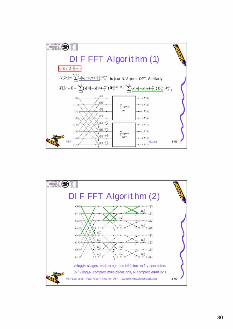
VSP Lecture6 - Fast Algorithms for DSP ([email protected]) 3-59
DIF FFT Algorithm (1)
is just N/2-point DFT. Similarly,
VSP Lecture6 - Fast Algorithms for DSP ([email protected]) 3-60
DIF FFT Algorithm (2)
v=log2N stages, each stage has N/2 butterfly operation.
(N/2)log2N complex multiplications, N complex additions

31
VSP Lecture6 - Fast Algorithms for DSP ([email protected]) 3-61
Remarks• The basic butterfly operations for DIT FFT and DIF FFT
respectively are transposed-form pair.
• The I/O values of DIT FFT and DIF FFT are the same• Applying the transpose transform to each DIT FFT
algorithm, one obtains DIF FFT algorithm
DIF BF unitDIT BF unit
VSP Lecture6 - Fast Algorithms for DSP ([email protected]) 3-62
Fast Convolution with the FFT• Given two sequences x1 and x2 of length N1 and N2
respectively– Direct implementation requires N1N2 complex
multiplications• Consider using FFT to convolve two sequences:
– Pick N, a power of 2, such that N≥N1+N2-1– Zero-pad x1 and x2 to length N– Compute N-point FFTs of zero-padded x1 and x2, then we
obtain X1 and X2– Multiply X1 and X2– Apply the IFFT to obtain the convolution sum of x1 and
x2– Computation complexity: 2(N/2) log2N + N + (N/2)log2N

32
VSP Lecture6 - Fast Algorithms for DSP ([email protected]) 3-63
Implementation Issues• Radix-2, Radix-4, Radix-8, Split-Radix,Radix-22, …, • I/O Indexing• In-place computation
– Bit-reversed sorting is necessary– Efficient use of memory– Random access (not sequential) of memory. An address
generator unit is required.– Good for cascade form: FFT followed by IFFT (or vice
versa)• E.g. fast convolution algorithm
• Twiddle factors– Look up table– CORDIC rotator
VSP Lecture6 - Fast Algorithms for DSP ([email protected]) 3-64
Algorithm Strength Reduction• Motivation
– The number of strong operations, such as multiplications, is reduced possibly at the expense of an increase in the number of weaker operations, such as additions.
• Reduce computation complexity• Example: Complex multiplication
– (a+jb)(c+jd)=e+jf, a,b,c,d,e,f ∈ R– The direct implementation requires 4 multiplications and 2
additions
– However, the number of multiplication can be reduced to 3 at the expense of 3 extra additions by using the identities
⎥⎦
⎤⎢⎣
⎡⎥⎦
⎤⎢⎣
⎡ −=⎥
⎦
⎤⎢⎣
⎡ba
cddc
fe
)()()()(
baddcbbcadbaddcabdac
−++=+−+−=− 3 multiplications
5 additions
33
VSP Lecture6 - Fast Algorithms for DSP ([email protected]) 3-65
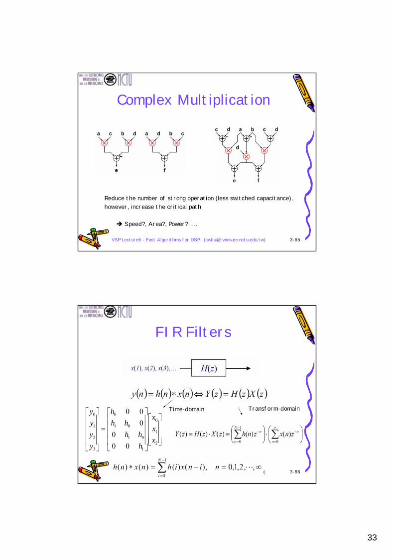
Complex Multiplication
Reduce the number of strong operation (less switched capacitance), however, increase the critical path
Speed?, Area?, Power? ….
VSP Lecture6 - Fast Algorithms for DSP ([email protected]) 3-66
FIR Filters
⎥⎥⎥
⎦
⎤
⎢⎢⎢
⎣
⎡
⎥⎥⎥⎥
⎦
⎤
⎢⎢⎢⎢
⎣
⎡
=
⎥⎥⎥⎥
⎦
⎤
⎢⎢⎢⎢
⎣
⎡
2
1
0
1
01
01
0
3
2
1
0
000
000
xxx
hhh
hhh
yyyy Transform-domainTime-domain
34
VSP Lecture6 - Fast Algorithms for DSP ([email protected]) 3-67
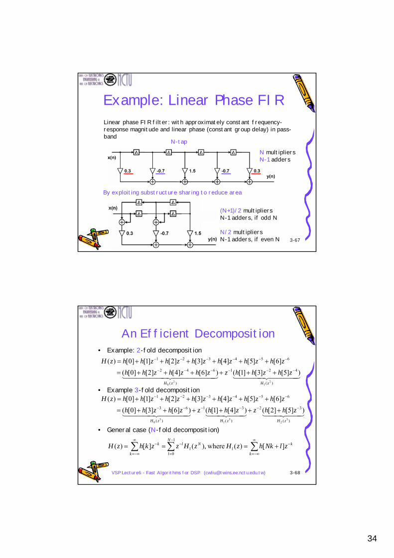
Example: Linear Phase FIRLinear phase FIR filter: with approximately constant frequency-response magnitude and linear phase (constant group delay) in pass-band
N-tap
N multipliersN-1 adders
(N+1)/2 multipliersN-1 adders, if odd N
N/2 multipliersN-1 adders, if even N
By exploiting substructure sharing to reduce area
VSP Lecture6 - Fast Algorithms for DSP ([email protected]) 3-68
An Efficient Decomposition• Example: 2-fold decomposition
• Example 3-fold decomposition
• General case (N-fold decomposition)
4444 34444 21444444 3444444 21)(
421
)(
642
654321
21
20
)]5[]3[]1[()]6[]4[]2[]0[( ]6[]5[]4[]3[]2[]1[]0[)(
zHzH
zhzhhzzhzhzhhzhzhzhzhzhzhhzH
−−−−−−
−−−−−−
++++++=
++++++=
44 344 2144 344 214444 34444 21)(
32
)(
31
)(
63
654321
32
31
30
)]5[]2[()]4[]1[()]6[]3[]0[( ]6[]5[]4[]3[]2[]1[]0[)(
zHzHzH
zhhzzhhzzhzhhzhzhzhzhzhzhhzH
−−−−−−
−−−−−−
++++++=
++++++=
∑∑∑∞
−∞=
−−
=
−∞
−∞=
− +===k
kl
N
l
Nl
l
k
k zlNkhzHzHzzkhzH ][)( where,)(][)(1
0
35
VSP Lecture6 - Fast Algorithms for DSP ([email protected]) 3-69
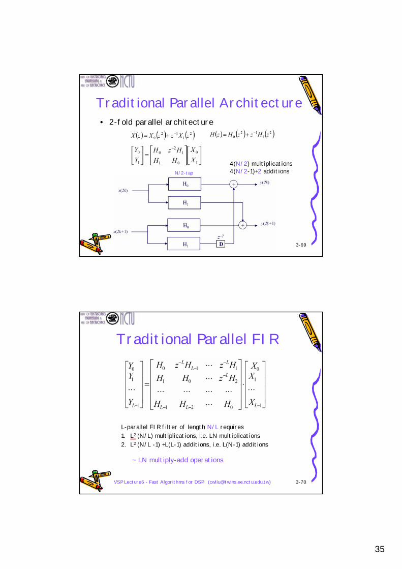
Traditional Parallel Architecture• 2-fold parallel architecture
4(N/2) multiplicationsN/2-tap 4(N/2-1)+2 additions
VSP Lecture6 - Fast Algorithms for DSP ([email protected]) 3-70
Traditional Parallel FIR
L-parallel FIR filter of length N/L requires 1. L2 (N/L) multiplications, i.e. LN multiplications2. L2 (N/L -1) +L(L-1) additions, i.e. L(N-1) additions
~ LN multiply-add operations
36
VSP Lecture6 - Fast Algorithms for DSP ([email protected]) 3-71
VSP Lecture6 - Fast Algorithms for DSP ([email protected]) 3-72
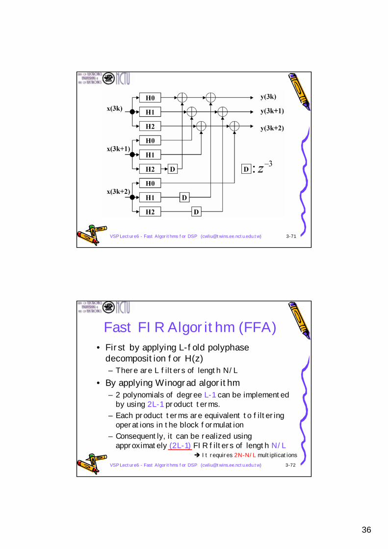
Fast FIR Algorithm (FFA)• First by applying L-fold polyphase
decomposition for H(z)– There are L filters of length N/L
• By applying Winograd algorithm– 2 polynomials of degree L-1 can be implemented
by using 2L-1 product terms.– Each product terms are equivalent to filtering
operations in the block formulation– Consequently, it can be realized using
approximately (2L-1) FIR filters of length N/LIt requires 2N-N/L multiplications