fast algorithms for hierarchically semiseparable matricescrd-legacy.lbl.gov/~xiaoye/fasthss.pdfhere,...

NUMERICAL LINEAR ALGEBRA WITH APPLICATIONSNumer. Linear Algebra Appl. 2010; 17:953–976Published online 22 December 2009 in Wiley Online Library (wileyonlinelibrary.com). DOI: 10.1002/nla.691

Fast algorithms for hierarchically semiseparable matrices

Jianlin Xia1,∗,†, Shivkumar Chandrasekaran2, Ming Gu3 and Xiaoye S. Li4

1Department of Mathematics, Purdue University, West Lafayette, IN 47907, U.S.A.2Department of Electrical and Computer Engineering, University of California, Santa Barbara, CA 93106, U.S.A.

3Department of Mathematics, University of California, Berkeley, CA 94720, U.S.A.4Lawrence Berkeley National Laboratory, MS 50F-1650, One Cyclotron Rd., Berkeley, CA 94720, U.S.A.

SUMMARY

Semiseparable matrices and many other rank-structured matrices have been widely used in developingnew fast matrix algorithms. In this paper, we generalize the hierarchically semiseparable (HSS) matrixrepresentations and propose some fast algorithms for HSS matrices. We represent HSS matrices in termsof general binary HSS trees and use simplified postordering notation for HSS forms. Fast HSS algorithmsincluding new HSS structure generation and HSS form Cholesky factorization are developed. Moreover,we provide a new linear complexity explicit ULV factorization algorithm for symmetric positive definiteHSS matrices with a low-rank property. The corresponding factors can be used to solve the HSS systemsalso in linear complexity. Numerical examples demonstrate the efficiency of the algorithms. All thesealgorithms have nice data locality. They are useful in developing fast-structured numerical methods forlarge discretized PDEs (such as elliptic equations), integral equations, eigenvalue problems, etc. Someapplications are shown. Copyright q 2009 John Wiley & Sons, Ltd.

Received 10 January 2009; Revised 11 November 2009; Accepted 13 November 2009

KEY WORDS: HSS matrix; postordering HSS tree; low-rank property; fast HSS algorithms; generalizedHSS Cholesky factorization

1. INTRODUCTION

Rank-structured matrices have attracted much attention in recent years. These matrices have beenshown very effective in solving linear systems [1–4], least squares problems [5], eigenvalueproblems [6–11], PDEs [12–15], integral equations [16–18], etc. Examples of rank-structuredmatrices include H-matrices [19–21], H2-matrices [22–24], quasiseparable matrices [25], andsemiseparable matrices [26–28]. It has been noticed that in the factorizations of some discretizedPDEs and integral equations, dense intermediate matrices have off-diagonal blocks with smallnumerical ranks. By exploiting this low-rank property, fast numerical methods can be developed.The property is also observed in some eigenvalue problems [6–8].∗Correspondence to: Jianlin Xia, Department of Mathematics, Purdue University, West Lafayette, IN 47907, U.S.A.†E-mail: [email protected]

Contract/grant sponsor: NSF; contract/grant numbers: CCF-0515034, CCF-0830764

Copyright q 2009 John Wiley & Sons, Ltd.

954 J. XIA ET AL.

Here, we consider a type of semiseparable structures called hierarchically semiseparable (HSS)matrices proposed in [1, 2, 29]. HSS structures have been used to develop fast direct or iterativesolvers for both dense and sparse linear systems [1, 2, 15, 29–31]. For dense matrices with thelow-rank property and represented in HSS forms, the linear system solution needs only linearcomplexity based on implicit ULV-type factorizations, where U and V are orthogonal matricesand L is lower-triangular [2, 29]. HSS matrices can also be used in many other applicationswhere the low-rank property exists. The HSS representation features a nice hierarchical multi-leveltree structure (HSS tree), and is efficient in capturing the semiseparable low-rank property. HSSstructures are closely related to H-matrices [19–21] and H2-matrices [22–24], and is a specialcase of the representations in the fast multipole method [18, 32, 33]. It is also a generalization ofthe sequentially semiseparable representation [5, 26].

In the meantime, the implementation of the current HSS algorithms is still not very convenient,partly due to the tedious notation and the level-wise (global) tree traversal scheme. Moreover, someexisting HSS algorithms can be highly improved, such as the structure construction and systemsolution, especially for symmetric problems.

Thus in this paper, we present simplifications and generalizations of HSS representations,which are easier to use and have better data locality. We also develop some HSS algorithms withbetter efficiency. With the improved HSS representation, most HSS algorithms can be done moreconveniently by traversing postordering HSS trees. Our generalizations of HSS structures alsoallow more flexibility in dealing with arbitrary HSS tree patterns.

The algorithms we propose can be used to provide nearly linear complexity direct solvers forsparse-discretized PDEs [15], such as elliptic equations and others [12–14, 34, 35]. Note that thesedense HSS techniques apply to discretized PDEs in one-dimensional (1D) domains, but can beused in sparse matrix schemes to work on 2D problems. For example, with the nested dissectionordering of a sparse discretized PDE followed by a multifrontal factorization, we can use HSSmatrices to approximate the dense intermediate fill-in [15]. Such a scheme can also possibly beused to solve or to precondition higher dimensional problems.

In addition, the postordering HSS tree notation we use simulates the assembly tree structure[36–38] in sparse matrix solutions and has a good potential to be parallelized. The ideas presentedhere are also useful for developing new HSS algorithms.

1.1. Review of HSS matrices

We first briefly review the standard HSS structure and give some concise definitions based on thediscussions in [1, 2, 15, 29–31].

The low-rank property is concerned with the ranks or numerical ranks of certain types of off-diagonal blocks. Here, by numerical ranks we mean the ranks obtained by rank revealing QRfactorizations or �-accurate SVD (SVD with an absolute or relative tolerance � for the singularvalues). The off-diagonal blocks used in HSS representations are called HSS blocks as shown inFigure 1(i), (ii). They are block rows or columns without diagonal parts and are hierarchicallydefined for different levels of splittings of the matrix.

Definition 1.1 (HSS blocks)

For an N×N matrix H and a partition sequence {mk; j }2kj=1 satisfying∑2k

i=1mk; j =N , partition H

into 2k block rows so that block row j has row dimension mk; j . Similarly, partition the columns.Denote the mk; j ×mk; j intersection block of block row j and block column j by Dk;i . Then,

Copyright q 2009 John Wiley & Sons, Ltd. Numer. Linear Algebra Appl. 2010; 17:953–976DOI: 10.1002/nla

FAST ALGORITHMS FOR HSS MATRICES 955

(1;2)(1;1)

(2;3)(2;2) (2;4)(2;1)

Figure 1. Two levels of HSS off-diagonal blocks: (i) first-level HSS blocks; (ii) second-level HSS blocks;and (iii) corresponding binary tree.

block row (column) j with Dk; j removed is called the j-th HSS block row (column) at the k-thlevel (bottom level) partition. Upper level HSS blocks are similarly defined using the partitionsequences {mi; j }2ij=1, which are given recursively by

mi−1; j =mi;2 j−1+mi;2 j , j =1,2, . . . ,2i−1−1,2i−1, i=k,k−1, . . . ,2,1.

Thus, the j th HSS block row at level i has dimensions mi; j ×(N−mi; j ). Clearly, these blockscan be associated with a binary tree. For example, we can have a binary tree as shown in Figure 1(iii)corresponding to Figure 1(i), (ii), where each tree node is associated with an HSS block row andcolumn. Later, we use (i; j) to denote the j-th node at level i of the tree.

Definition 1.2 (HSS tree and HSS representation)For a matrix H and its HSS blocks as defined in Definition 1.1, let T be a perfect binary tree whereeach node is associated with an HSS block row (column). H is said to have an HSS representationif there exists matrices Di; j , Ui; j , Vi; j , Ri; j , Wi; j , Bi; j, j±1 associated with each tree node (i; j)which satisfy the recursions

Di−1; j =(

Di;2 j−1 Ui;2 j−1Bi;2 j−1,2 j VTi;2 j

Ui;2 j Bi;2 j,2 j−1VTi;2 j−1 Di;2 j

),

Ui−1; j =(Ui;2 j−1Ri;2 j−1

Ui;2 j Ri;2 j

), Vi−1; j =

(Vi;2 j−1Wi;2 j−1

Vi;2 jWi;2 j

),

j=1,2, . . . ,2i−1−1,2i−1, (1)

i=k, k−1, . . . ,2,1,

so that D0;1≡H , corresponding to the root of T. The matrices in (1) are called generators of H .If node (i; j) of T is associated with the generators Di; j , Ui; j , Vi; j , Ri; j , Wi; j , Bi; j, j±1, we sayT is an HSS tree of H .


956 J. XIA ET AL.

B1;1,2

B1;2,1(1;2)

W2;2

R2;2R2;1

W2;1

B2;1,2

B2;2,1

(1;1)

(2;3)(2;2) (2;4)(2;1)

U2;2, V2;2U2;1, V2;1

W2;4

R2;4R2;3

W2;3

B2;4,3

B2;3,4

U2;4, V2;4U2;3, V2;3D2;1 D2;2 D2;3 D2;4

Figure 2. HSS tree for (2).

Note that due to this hierarchical structure, only R, W generators and bottom level D, U , Vgenerators need to be stored. As an example, a block 4×4 HSS matrix looks like

m2;1m2;2m2;3m2;4

⎛⎜⎜⎜⎜⎜⎝

(D2;1 U2;1B2;1,2V T

2;2U2;2B2;2,1V T

2;1 D2;2

) (U2;1R2;1U2;2R2;2

)B1;1,2(WT

2;3VT2;3 WT

2;4VT2;4)

(U2;3R2;3U2;4R2;4

)B1;2,1(WT

2;1VT2;1 WT

2;2VT2;2)

(D2;3 U2;3B2;3,4V T

2;4U2;4B2;4,3V T

2,3 D2;4

)⎞⎟⎟⎟⎟⎟⎠ ,

(2)

which corresponds to the second-level block partition in Figure 1. The hierarchical structure ofHSS matrices can be seen by writing (2) in terms of the first-level block partition

m1;1≡m2;1+m2;2m1;2≡m2;3+m2;4

(D1;1 U1;1B1;1,2V T

1;2U1;2B1;2,1V T

1;1 D1;2

). (3)

The corresponding HSS tree of H is shown in Figure 2.HSS trees can be used to conveniently represent HSS matrices. As an example, the (2,3) block

of (2) can be identified by the directed path connecting the second and third nodes at level 2:

U2;2(2;2) R2;2−→(1;1) B1;1,2−→(1;2) WT

2;3−→V T2;3

(2;3),where U and R generators are used for outgoing directions, and V and W generators are used forincident directions. HSS trees also allow the operations on HSS matrices to be done convenientlyvia tree operations.

In addition, we can see that the second-level HSS block rows in (2) are given by

U2;1(B2;1,2 R2;1B1;1,2)diag(V T2;2,V

T1;2), U2;2(B2;2,1 R2;2B1;1,2)diag(V T

2;2,VT1;2), etc.,

where each U2;i is an appropriate column basis matrix and diag(V T2;2,V

T1;2) (denoting a diagonal

matrix formed with diagonal blocks V T2;2 and V T

1;2) is a row basis.The effectiveness of HSS structures relies on the low-rank property.

Definition 1.3 (low-rank property)A matrix with given partition sequences as in Definition 1.1 is said to have the low-rank property(in terms of HSS blocks) if all its HSS blocks have small ranks or numerical ranks.



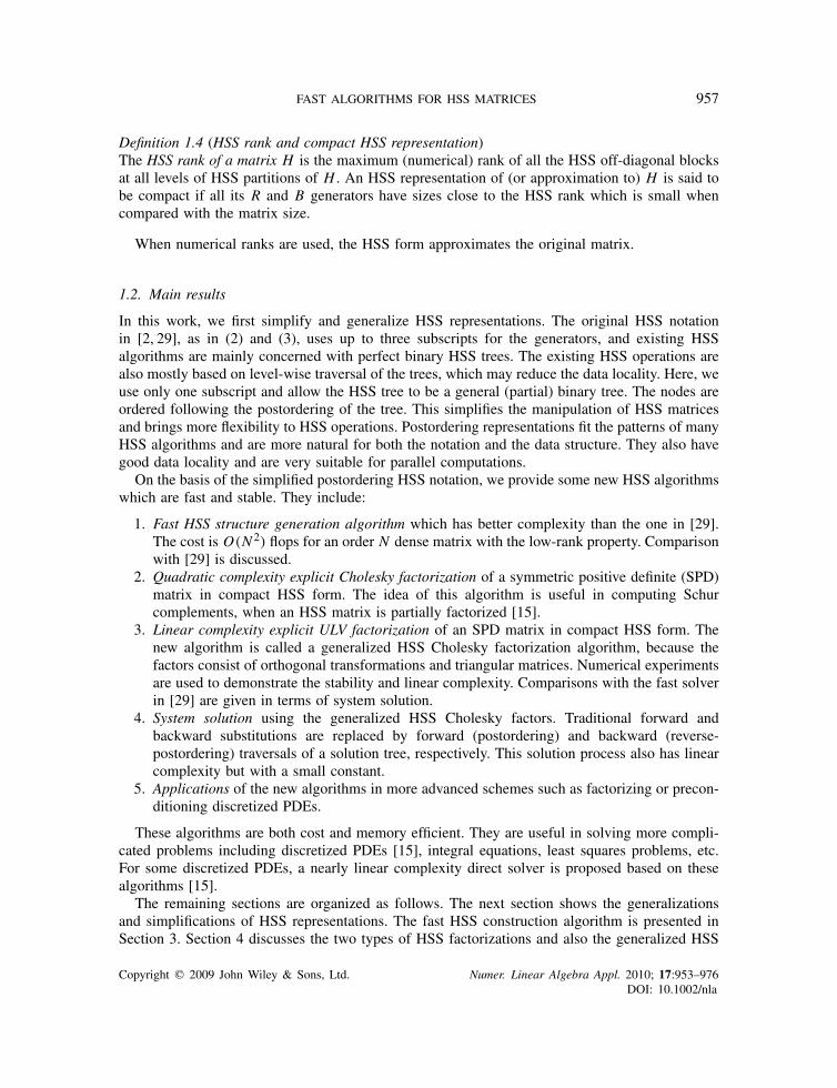
Definition 1.4 (HSS rank and compact HSS representation)The HSS rank of a matrix H is the maximum (numerical) rank of all the HSS off-diagonal blocksat all levels of HSS partitions of H . An HSS representation of (or approximation to) H is said tobe compact if all its R and B generators have sizes close to the HSS rank which is small whencompared with the matrix size.

When numerical ranks are used, the HSS form approximates the original matrix.

1.2. Main results

In this work, we first simplify and generalize HSS representations. The original HSS notationin [2, 29], as in (2) and (3), uses up to three subscripts for the generators, and existing HSSalgorithms are mainly concerned with perfect binary HSS trees. The existing HSS operations arealso mostly based on level-wise traversal of the trees, which may reduce the data locality. Here, weuse only one subscript and allow the HSS tree to be a general (partial) binary tree. The nodes areordered following the postordering of the tree. This simplifies the manipulation of HSS matricesand brings more flexibility to HSS operations. Postordering representations fit the patterns of manyHSS algorithms and are more natural for both the notation and the data structure. They also havegood data locality and are very suitable for parallel computations.

On the basis of the simplified postordering HSS notation, we provide some new HSS algorithmswhich are fast and stable. They include:

1. Fast HSS structure generation algorithm which has better complexity than the one in [29].The cost is O(N 2) flops for an order N dense matrix with the low-rank property. Comparisonwith [29] is discussed.

2. Quadratic complexity explicit Cholesky factorization of a symmetric positive definite (SPD)matrix in compact HSS form. The idea of this algorithm is useful in computing Schurcomplements, when an HSS matrix is partially factorized [15].

3. Linear complexity explicit ULV factorization of an SPD matrix in compact HSS form. Thenew algorithm is called a generalized HSS Cholesky factorization algorithm, because thefactors consist of orthogonal transformations and triangular matrices. Numerical experimentsare used to demonstrate the stability and linear complexity. Comparisons with the fast solverin [29] are given in terms of system solution.

4. System solution using the generalized HSS Cholesky factors. Traditional forward andbackward substitutions are replaced by forward (postordering) and backward (reverse-postordering) traversals of a solution tree, respectively. This solution process also has linearcomplexity but with a small constant.

5. Applications of the new algorithms in more advanced schemes such as factorizing or precon-ditioning discretized PDEs.

These algorithms are both cost and memory efficient. They are useful in solving more compli-cated problems including discretized PDEs [15], integral equations, least squares problems, etc.For some discretized PDEs, a nearly linear complexity direct solver is proposed based on thesealgorithms [15].

The remaining sections are organized as follows. The next section shows the generalizationsand simplifications of HSS representations. The fast HSS construction algorithm is presented inSection 3. Section 4 discusses the two types of HSS factorizations and also the generalized HSS


958 J. XIA ET AL.

solver. Numerical experiments are included. Some applications of these HSS algorithms are shownin Section 5. Section 6 gives some concluding remarks.

2. GENERALIZATIONS OF HSS REPRESENTATIONS

In this section, we first simplify the HSS notation and then introduce partial HSS forms.

2.1. Postordering HSS representation

Tree structures are very useful in numerical problems like direct solutions of sparse linear systemswhere they appear as assembly trees [36–38]. In an assembly tree, the nodes are often orderedfollowing the postordering, which gives the actual elimination order. Similarly in the situation ofHSS operations, it often needs to traverse HSS trees. A postordering of the HSS tree nodes bringsmore flexibility and convenience.

For example, the nodes of the HSS tree in Figure 2 can be relabeled in the postordering formas in Figure 3(i). Accordingly, the generators are relabeled with only one index each. We callthis HSS notation the postordering HSS notation. Accordingly, the HSS off-diagonal blocks atdifferent levels are also ordered and associated with the tree nodes. With the postordering notation,the matrix (2) now looks like

⎛⎜⎜⎜⎜⎜⎝

D1 U1B1VT2 U1R1B3W

T4 V

T4 U1R1B3W

T5 V

T5

U2B2VT1 D2 U2R2B3W

T4 V

T4 U2R2B3W

T5 V

T5

U4R4B6WT1 V

T1 U4R4B6W

T2 V

T2 D4 U4B4V

T5

U5R5B6WT1 V

T1 U5R5B6W

T2 V

T2 U5B5V

T4 D5

⎞⎟⎟⎟⎟⎟⎠ . (4)

The postordering HSS notation simplifies the HSS representation and is convenient in HSSstructure transformations, data manipulations, parallelization, etc. Moreover, the postordering HSSrepresentation keeps good data locality by limiting direct communications to be between parentand child nodes only.

B3

B66

W2

R2R1

W1

B1

B2

3

42 51

U2, V2U1, V1

W5

R5R4

W4

B4

B5

U5, V5U4, V4

D1 D2 D4 D5

7 7

B3

B663

4 5

U3, V3W5

R5R4

W4

B4

B5

U5, V5U4, V4

D3

D4 D5

7

B3

B66

W2

R2

3

42 5

U2, V2

W5

R5R4

W4

B4

B5

U5, V5U4, V4

D2 D4 D5

Figure 3. Examples of a postordering HSS tree and partial HSS trees: (i) postordering form of Figure 2;(ii) full HSS tree; and (iii) general partial HSS tree.



2.2. Partial HSS form

In Figure 3(i), the HSS tree is a perfect binary tree, that is, the tree has 2l+1−1 nodes if it hasl levels (the root is at level 0). But HSS trees can be more general. For example, if we mergethe first two block rows and columns of the matrix (4), we get an HSS form corresponding toFigure 3(ii). We may have even more general cases like Figure 3(iii).

An HSS tree which is not perfect is said to be a partial HSS tree, and the corresponding HSSmatrix is in partial HSS form. In various HSS operations like solving HSS systems, it is often moreconvenient and practical to use partial HSS trees [15]. Thus, we consider operations on generalpartial HSS matrices, not necessarily restricted to complete HSS matrices as in [29]. However, atree in Figure 3(iii) can be transformed to Figure 3(ii) by merging certain nodes and edges, so itusually suffices to consider partial HSS trees which are full binary trees. That is, each non-leafnode i has two children c1 and c2 with c1<c2, called the left and right children of i , respectively.Furthermore, it suffices to use full binary trees due to the following simple fact.

Theorem 2.1For any integer k>0, there always exists a full binary tree with exactly k leaf nodes and 2k−1nodes in total.

ProofA straightforward proof is to construct an unbalanced full binary tree where each right (or left)node is only a leaf node . Such a tree with k leaves has exactly k−1 non-leaf nodes. A generallybetter choice is to recursively construct a tree, which is as balanced as possible or has as smalldepth as possible. �

3. FAST AND STABLE CONSTRUCTION OF HSS REPRESENTATIONS

For a dense matrix H and a partition sequence {mi }, there always exists a full HSS tree accordingto Theorem 2.1. We assume that an HSS tree corresponding to {mi } is also given. The paper [29]provides an HSS construction algorithm based on (�-accurate) SVDs. That method traverses HSStrees by levels and, in general, can only generate HSS matrices with perfect HSS trees. Here, weprovide a new algorithm which follows a general postordering (partial) HSS tree. It is fully stableand costs much less than the one in [29]. We compress the HSS off-diagonal blocks associated withthe tree nodes. Here, by compression we mean a QR factorization or SVD of a low-rank block,or a rank-revealing QR or �-accurate SVD of a numerically low-rank block when approximationsare used.

3.1. A block 4×4 example

We first demonstrate the procedure of constructing a 4×4 block HSS form (4) for H using thepostordering HSS tree in Figure 3. Initially, we partition the matrix H into a 4×4 block form

H =

⎛⎜⎜⎜⎜⎝

D1 T12 T14 T15

T21 D2 T24 T25

T41 T42 D4 T45

T51 T52 T54 D5

⎞⎟⎟⎟⎟⎠ ,


960 J. XIA ET AL.

where the subscripts follow the node ordering, that is Tij denotes the block corresponding to nodesi and j . Moreover, we use Ti,: (T:,i ) to denote the HSS block row (column) corresponding to nodei . As an example, the HSS block rows corresponding to nodes 1 and 3 are T1,: ≡(T12 T14 T15) and

T3,: ≡(T14 T15

T24 T25

),

respectively. The HSS construction is done following the traversal of the HSS tree. We demonstratethe first few steps.

(a) Node 1. At the beginning, we compress the HSS off-diagonal block row and columncorresponding to node 1 by QR factorizations

T1,:(≡(T12 T14 T15)) =U1(T12 T14 T15),

T T:,1(≡(T T21 T T

41 T T51)) = V1(T

T21 T T

41 T T51),

where Tij denotes a temporary matrix (so does Tij below).(b) Node 2. Now, compress the HSS block row and column for node 2. Parts of these blocks have

been compressed in the previous step. As U and V matrices are bases of appropriate off-diagonalblocks, the compression of those blocks can be done without these basis matrices. For example,this can be justified by writing

T2,: =(T21VT1 T24 T25)=(T21 (T24 T25))

(V T1

I

).

Thus, V T1 can be ignored in further compressions. This is essential in saving the cost. Compute

QR factorizations

(T21 T24 T25) =U2(B2 T24 T25),

(T T12 T T

42 T T52) = V2(B

T1 T T

42 T T52).

Then H becomes

H =

⎛⎜⎜⎜⎜⎜⎝

D1 U1B1VT2 U1T14 U1T15

U2B2VT1 D2 U2T24 U2T25

T41VT1 T42V

T2 D4 T45

T51VT1 T52V

T2 T54 D5

⎞⎟⎟⎟⎟⎟⎠ .

(c) Node 3. The HSS block row and column corresponding to node 3 can be obtained by mergingappropriate pieces of the HSS blocks of nodes 1 and 2 (Figure 1). We identify and compress them(ignoring any U , V -bases)(

T14 T15

T24 T25

)=(R1

R2

)(T34 T35),

(T T41 T T

51

T T42 T T

52

)=(W1

W2

)(T T

43 T T53).

H then has a more compact form.



Similarly, we can continue the compression of the HSS blocks, but with appropriate U , V -basesignored in the QR factorizations.

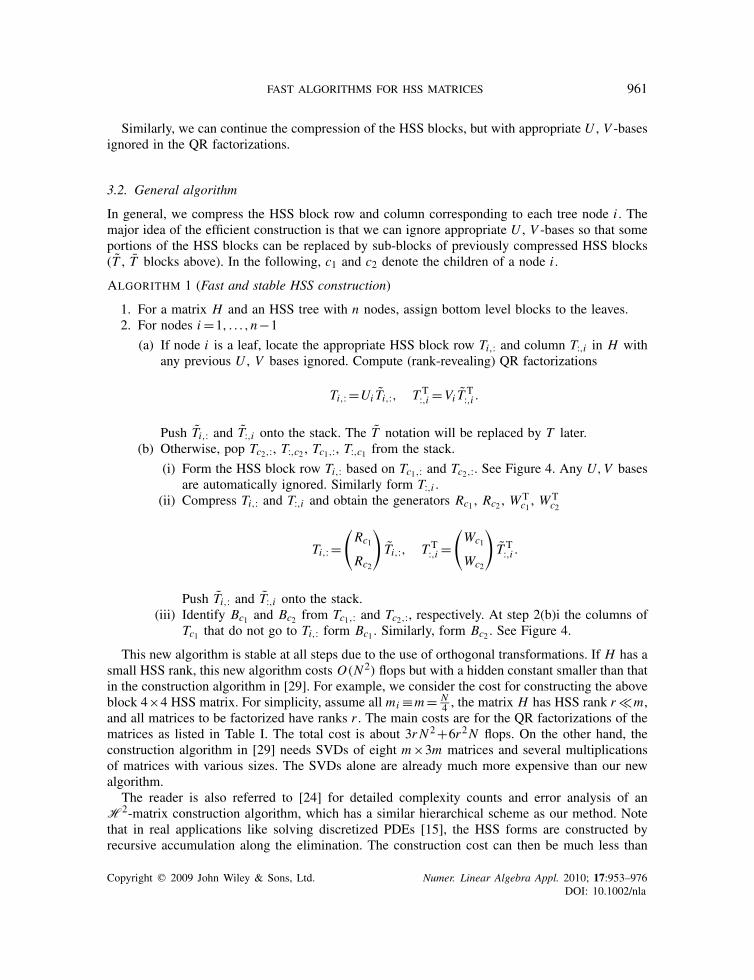
3.2. General algorithm

In general, we compress the HSS block row and column corresponding to each tree node i . Themajor idea of the efficient construction is that we can ignore appropriate U , V -bases so that someportions of the HSS blocks can be replaced by sub-blocks of previously compressed HSS blocks(T , T blocks above). In the following, c1 and c2 denote the children of a node i .

ALGORITHM 1 (Fast and stable HSS construction)

1. For a matrix H and an HSS tree with n nodes, assign bottom level blocks to the leaves.2. For nodes i=1, . . . ,n−1

(a) If node i is a leaf, locate the appropriate HSS block row Ti,: and column T:,i in H withany previous U , V bases ignored. Compute (rank-revealing) QR factorizations

Ti,: =Ui Ti,:, T T:,i =Vi TT:,i .

Push Ti,: and T:,i onto the stack. The T notation will be replaced by T later.(b) Otherwise, pop Tc2,:, T:,c2 , Tc1,:, T:,c1 from the stack.

(i) Form the HSS block row Ti,: based on Tc1,: and Tc2,:. See Figure 4. Any U,V basesare automatically ignored. Similarly form T:,i .

(ii) Compress Ti,: and T:,i and obtain the generators Rc1 , Rc2 , WTc1 , W

Tc2

Ti,: =(Rc1

Rc2

)Ti,:, T T:,i =

(Wc1

Wc2

)T T:,i .

Push Ti,: and T:,i onto the stack.(iii) Identify Bc1 and Bc2 from Tc1,: and Tc2,:, respectively. At step 2(b)i the columns of

Tc1 that do not go to Ti,: form Bc1 . Similarly, form Bc2 . See Figure 4.

This new algorithm is stable at all steps due to the use of orthogonal transformations. If H has asmall HSS rank, this new algorithm costs O(N 2) flops but with a hidden constant smaller than thatin the construction algorithm in [29]. For example, we consider the cost for constructing the aboveblock 4×4 HSS matrix. For simplicity, assume all mi ≡m= N

4 , the matrix H has HSS rank r �m,and all matrices to be factorized have ranks r . The main costs are for the QR factorizations of thematrices as listed in Table I. The total cost is about 3r N 2+6r2N flops. On the other hand, theconstruction algorithm in [29] needs SVDs of eight m×3m matrices and several multiplicationsof matrices with various sizes. The SVDs alone are already much more expensive than our newalgorithm.

The reader is also referred to [24] for detailed complexity counts and error analysis of anH2-matrix construction algorithm, which has a similar hierarchical scheme as our method. Notethat in real applications like solving discretized PDEs [15], the HSS forms are constructed byrecursive accumulation along the elimination. The construction cost can then be much less than


962 J. XIA ET AL.

Figure 4. Forming Ti,: and identifying Bc1 and Bc2 .

Table I. Matrices for QR factorizations in the construction of the block 4×4 HSS matrix example.

Matrix size m×3m r×(2r+r) 2r×2m m×(m+r) m×2r 2m×rNumber of matrices 2 2 2 2 2 2

O(N 2). It is also possible to generalize HSS constructions to higher dimensional problems usingthe techniques in [24].

4. FAST QUADRATIC COMPLEXITY AND LINEAR COMPLEXITY HSSFACTORIZATIONS

In this section, we discuss explicit factorizations of HSS matrices. For simplicity, we only considerSPD matrices. We look at two types of factorizations: the Cholesky factorization of an SPD HSSmatrix and a generalized HSS Cholesky factorization.

4.1. Fast Cholesky factorization of SPD HSS matrices

Given the HSS form of an SPD matrix, we can conveniently compute its HSS form Choleskyfactor. As the matrix is symmetric, the generators satisfy

DTi =Di , Ui =Vi , Ri =Wi , and Bi = BT

j for siblings i and j.

Assume H has an HSS tree like Figure 3(i) but with more nodes. The factorization consists of twomajor operations, eliminating the principal diagonal block and updating the Schur complement.Correspondingly, there are two operations on the HSS tree: removing a node and updating theremaining ones.

First, we look at the situation of eliminating node 1. Factorize D1= L1LT1 and compute the

Schur complement H as follows:

H =(L1 0

l1 I

)(LT1 lT1

0 H

),



where

lT1 = (U1B1UT2 U1R1B3R

T4U

T4 U1R1B3R

T5U

T5 . . .),

H =

⎛⎜⎜⎜⎜⎜⎜⎝

D2 U2 R2B3RT4U

T4 U2 R2B3R

T5U

T5 . . .

U4R4BT3 R

T2U

T2 D4 U4 B4U

T5 . . .

U5R5BT3 R

T2U

T2 U5 B

T4U

T4 D5

......

. . .

⎞⎟⎟⎟⎟⎟⎟⎠

,

with U1= L−11 U1 and

D2 = D2−U2BT1 U

T1 U1B1U

T2 , R2= R2−BT

1 UT1 U1R1

D4 = D4−U4R4BT3 R

T1 U

T1 U1R1B3R

T4U

T4 , B4= B4−R4B

T3 R

T1 U

T1 U1R1B3R

T5 , . . .

We can see that the Schur complement H takes a form similar to the original matrix but with itsfirst block row and column removed.

In general, the update of the generators can be clearly seen by using appropriate paths in thetree. Following the postordering of the nodes i=1, . . . ,n, we can perform two steps to removeeach node i during the elimination. At the first step, eliminate node i by computing

Di = Li LTi , Di = Li , Ui = L−1

i Ui .

At the second step, compute the Schur complement by updating the remaining nodes. This means,we consider each node j = i+1, . . . ,n according to the rules below.

1. If node j is a leaf node, locate the path connecting j and i : j →···→ i→···→ j , and updateDj as

D j =Dj −Uj R j . . . RTi U

Ti Ui Ri . . . R

Tj U

Tj .

2. If node j is a left child, locate the path connecting j to i and then to s, the sibling of j :j →···→ i → . . .→s, and update Bj as

B j = Bj −R j . . . RTi U

Ti Ui Ri . . . R

Ts .

3. If node j is the right child of p which is an ascendant of i , locate the path connecting j toi and then to s, the sibling of j : j →···→ i →···→s, and update R j as

R j = R j −BTs . . . RT

i UTi Ui Ri . . . Rs .

Nodes of the HSS tree are removed along the progress of the elimination. This algorithm givesan explicit HSS form of the Cholesky factor. The idea is also useful for finding Schur complementsin partial HSS factorizations [15]. This algorithm costs O(N 2) flops where N is the dimensionof H . As our main concern is the linear complexity factorization below, we skip the detailed flopcount.


964 J. XIA ET AL.

4.2. Linear complexity generalized Cholesky factorization of HSS matrices

There exist O(N ) complexity algorithms for solving a compact HSS system [29]. The HSS solverin [29] computes an implicit ULV factorization. However, sometimes an explicit factorization ofan HSS matrix may be convenient. Furthermore, various simplifications and improvements can bemade. Here, we provide an improved linear complexity factorization scheme. As our algorithmcomputes an explicit ULV factorization instead of the traditional Cholesky factorization, we callit a generalized HSS Cholesky factorization. In the following, we factorize a compact SPD HSSmatrix H such as the one represented by the HSS tree in Figure 3(i).

4.2.1. Introducing zeros into off-diagonal blocks. We consider to partially eliminate node i in theHSS tree. The generator Ui is a basis matrix for the i-th off-diagonal block row. It is directlyavailable for any leaf node i , and can be formed recursively for a non-leaf node. By bringing zerosinto Ui , we can quickly introduce zeros into the HSS blocks corresponding to i .

Assume that Ui has size mi ×ki . In a compact HSS form, we should have mi�ki . Here, weleave the case mi =ki to Subsection 4.2.3 and assume mi>ki . In such a situation, we can introducea QL factorization with an orthogonal transformation Qi such that

Ui =Qi

(0

Ui

), Ui :ki ×ki . (5)

Multiply QTi to the entire block row i . Then the first mi −ki rows of the off-diagonal block

become zeros. See Figure 5 for a pictorial representation. Similarly, we apply Qi on the right tothe off-diagonal column corresponding to node i . As the HSS form is symmetric, this will alsointroduce mi −ki zero columns in the i-th off-diagonal block column. The diagonal block is nowchanged to

Di =QTi Di Qi . (6)

D1

D2

D4

D5

Q1T

U1

U3

D1

D2

D4

D5

Figure 5. A pictorial representation for introducing zeros into the off-diagonal block rows of an HSSmatrix. Dark blocks represent the nonzero portions of the generators in the block upper triangular part.

The nonzero pattern for the block lower triangular part comes from symmetry and is not shown.



Figure 6. Partial factorization of a diagonal block and merging generators of siblings: (i) partial factor-ization; (ii) after partial elimination; and (iii) merging blocks.

4.2.2. Partially factorizing diagonal blocks. We partition the diagonal block Di conformally andpartially factorize it

Di =(mi −ki ki

mi −ki Di;1,1 Di;1,2ki Di;2,1 Di;2,2

)=(

Li 0

Di;2,1L−Ti I

)(LTi L−1

i Di;1,20 Di

), (7)

where Di is the Schur complement

Di =Di;2,2−Di;2,1L−Ti L−1

i Di;1,2. (8)

See Figure 6(i). We see that the block Di;1,1 can then be eliminated (Figure 6(ii)).

4.2.3. Merging child blocks. At this point, Ui is a square matrix (corresponding to the situationmi =ki mentioned in Subsection 4.2.1). We then merge sibling blocks and move to the parentnode (instead of doing level-wise elimination as in [29]). For notational convenience, we use i tomean a parent node, with its children c1 and c2 partially eliminated as above. Then, we can mergeblocks to obtain upper level generators

Di =(

Dc1 Uc1Bc1UTc2

Uc2BTc1U

Tc1 Dc2

), Ui =

(Uc1Rc1

Uc2Rc2

). (9)

We emphasize that these Di and Ui are the generators of the reduced HSS matrix, instead of theoriginal H .

Now, we can remove nodes c1 and c2 from the HSS tree. We repeat these steps followingthe postordering of the tree to eliminate other nodes, until we reach the root n where we canfactorize its reduced-size Dn generator directly. Note that a node only communicates with itsparent (and children). This is essential for the linear complexity of the factorization and is usefulfor parallelization.


966 J. XIA ET AL.

4.2.4. Algorithm and complexity. We organize the steps in the following algorithm.

ALGORITHM 2 (Generalized HSS Cholesky factorization)

1. Let H be an SPD HSS matrix with n nodes in the HSS tree. Allocate space for a stack.2. For each node i=1,2, . . . ,n−1

(a) If i is a non-leaf node

(i) Pop Dc2 , Uc2 , Dc1 , Uc1 from the stack, where c1,c2 are the children of i .(ii) Obtain Di and Ui with (9).

(b) Compress Ui with (5). Push Ui onto the stack.(c) Update Di with (6). Factorize Di with (7) and obtain the Schur complement Di as in

(8). Push Di onto the stack.

3. For the root node n, form Dn and compute the Cholesky factorization Dn = LnLTn .

Remark 1For each step, we can also replace the compression step (5) and the partial Cholesky factorizationstep (7) by a different process. That is, we first compute a full Cholesky factorization Di = Li LT

i

and then QR factorize L−1i Ui . This way, Di is updated to an identity matrix and remains so that

step (6) is avoided, which can save some work.

Note that the factors after the generalized Cholesky factorization include lower triangularmatrices Li , orthogonal transformations Qi in the compressions, and applicable permutations Piduring the merge step. They together form the generalized HSS Cholesky factor. To clearly seethe roles of these matrices in the actual factorization, we look at an example with three nodes inthe tree. The off-diagonal compression and the partial diagonal factorization leads to

H =(Q1 0

0 Q2

)L3

⎛⎜⎜⎜⎜⎜⎝

(I 0

0 D1

) (0 0

0 U1B1UT2

)(0 0

0 U2BT1 U

T1

) (I 0

0 D2

)⎞⎟⎟⎟⎟⎟⎠ LT

3

(QT

1 0

0 QT2

),

where the notation I for identity matrices and 0 for zero matrices may have different sizes, and

L3=diag

((L1 0

T1 I

),

(L2 0

T2 I

))with T1=D1;2,1L−T

1 , T2=D2;2,1L−T2 . (10)

The merge process then uses a permutation matrix P3 to bring together appropriate dense blocksto form D3 as shown in (9) (there is no U3 as there are only two bottom-level blocks here). Thenanother factorization step D3= L3LT

3 follows. Thus,

H = LH LTH with LH =Q3 L3P3

(I 0

0 L3

). (11)

The matrix LH is the actual generalized HSS Cholesky factor formed by {Li }, {Ti }, {Qi }, and{Pi }. This procedure is recursive and we can easily generalize the example. In addition, Qi andPi can be stored in terms of (Householder) vectors and scalars (matrix dimensions), respectively.



Table II. Flop counts of some basic matrix operations, with low-order terms dropped.

Operation Flops

Cholesky factorization of an n×n matrix n3/3Inverse of an n×n lower triangular matrix times an n×k matrix n2kQR factorization of an m×k tall matrix (m>k) 2k2(m− k

3 )

Product of Q and an m×n vector 2nk(2m−k)Product of a general m×n matrix and an n×k matrix 2mnk

Table III. Sizes of the generators in Algorithm 2, where i and j are siblings.

Generator Ui Ri BiSize mi ×ki ki ×kp ki ×k j

The algorithm has linear complexity as shown in the following theorem.

Theorem 4.1Assume that an N×N SPD matrix H is in compact HSS form with a full HSS tree. Moreover,assume that the bottom-level HSS block row dimensions are O(r), where r is the HSS rank ofH . Then the generalized Cholesky factorization of H with Algorithm 2 has complexity O(r2N )

flops.

ProofTo show the complexity, we use the flop counts of some basic matrix operations as listed inTable II. They can be found, say, in [39, 40].

Consider node i of the HSS tree corresponding to each step i of Algorithm 2. Assume node i(except the root) has a sibling j , a parent p, and two children c1 and c2 if applicable. We furtherassume the Ui basis being compressed in (5) has dimension mi ×ki . Note that for a non-leaf i , thematrices Di and Ui are generators of a reduced HSS matrix after an intermediate merge process(9), and is not a generator of the original H . This means, each Ui in the compression step (5) hasrow dimension mi =O(r). Also, let Ri and Bi have dimensions as indicated in Table III. Clearly,all ki =O(r).

The major operations in the factorization are as follows.

• For a non-leaf i , the merge step (9) needs four matrix-matrix products Uc1Bc1 , (Uc1Bc1)UTc2 ,

Uc1Rc1 , and Uc2Rc2 , with costs 2mc1kc1kc2 , 2mc1kc2mc2 , 2mc1kc1ki , and 2mc2kc2ki , respec-tively.

• For each i , the compression (QR) step (5) costs 2k2i (mi − ki3 ).

• For each i , the diagonal update (6) costs 4miki (2mi −ki ) due to two products involving Qi .• For each i , the partial factorization in (7) costs 1

3 (mi −ki )3, (mi −ki )2ki , and (mi −ki )k2i ,which are for factorizing the pivot block, updating the lower triangular part, and computingthe Schur complement, respectively.

These counts are summarized in the third column of Table IV.To simplify the calculations, we assume each bottom-level Ui has the same row dimension m.

The counts are then simplified as in the third column of Table IV. The HSS tree has N/m leaf


968 J. XIA ET AL.

Table IV. Cost of generalized HSS Cholesky factorization (leading terms only).

Node Operation Flops Number of nodes

Leaf Compression (5) 2k2i (mi − ki3 ) =O(mr2) ×N/m

node i Diagonal update (6) 4miki (2mi −ki ) =O(m2r)Factorization (7) 1

3 (mi −ki )3+(mi −ki )

2ki+(mi −ki )k

2i =O((m−r)3)

Non-leaf Merge step (9) 2(mc1kc1kc2 +mc1kc2mc2 ×(N/m−1)node i +mc1kc1ki +mc2kc2ki ) =O(r3)

Diagonal update (6) 4miki (2mi −ki ) =O(r3)Compression (5) 2k2i (mi − ki

3 ) =O(r3)

Factorization (7) 13 (mi −ki )

3+(mi −ki )2ki

+(mi −ki )k2i =O(r3)

Table V. Computation time (in seconds) of the generalized HSS Cholesky factorization and system solution(denoted NEW), when compared with DPOTRF, where × means insufficient memory.

Matrix size 256 512 1024 2048 4096 8192 16 384

DPOTRF 0.074 0.765 11.339 105.068 845.855 6857.316 ×NEW Factorization 0.068 0.076 0.104 0.172 0.280 0.520 0.953

Solution 0.003 0.006 0.013 0.029 0.054 0.109 0.227

Matrix size 32 768 65 536 131 072 262 144 524 288 1 048 576

DPOTRF × × × × × ×NEW Factorization 1.855 3.773 7.453 14.914 32.797 59.547

Solution 0.457 0.871 1.746 3.566 7.211 13.875

nodes, and N/m−1 non-leaf nodes. Therefore, the total cost is

[O(mr2)+O(m2r)+O((m−r)3)]× N

m+O(r3)× N

m=O(r2N ),

as m=O(r). �

Numerical experiments for the algorithm are displayed in Table V of Subsection 4.4 togetherwith system solution results.

4.3. HSS linear system solver with the generalized HSS Cholesky factor

After we compute generalized Cholesky HSS factorization, we can solve HSS systems withsubstitutions. Assume we solve the system Hx=b, where H = LH LT

H and the generalized Choleskyfactor LH is formed by {Li }, {Ti }, {Qi }, {Pi } as obtained in Algorithm 2. Just like the traditionaltriangular system solution, our new HSS solver also has two stages, forward substitution andbackward substitution, for the following two systems, respectively

LH y = b, (12)

LTH x = y. (13)



Here, the substitutions are done along the HSS tree, following the postordering (or bottom-up,forward) and reverse-postordering (or top-down, backward) traversals, respectively.

4.3.1. Forward substitution. We solve (12) first. If we have, say, an explicit expression like (11),then we can explicitly write

y=(I 0

0 L−13

)PT3 L

−13

(QT

1 0

0 QT2

)b (14)

which involves matrix–vector multiplications and standard triangular system solution. But ingeneral, we do this implicitly with the HSS factorization tree whose structure has good data locality.The solution vector y is obtained in the following way.

We use the space of b for y. First, partition b conformally according to the bottom-level blocksizes or the partition sequence {mi }. Denote the vector pieces by {yi }. Associate yi with eachleaf i .

Next, apply QTi to yi (see (14))

yi =QTi yi =

mi −ri

ri

(yi;1yi;2

),

where yi is partitioned according to (5) and (7). Then, we solve for

yi =(Li 0

Ti I

)−1

yi =(

yi;1yi;2−Ti yi;1

)≡mi −ri

ri

(yi;1yi;2

), (15)

where yi;1= L−1i yi;1. The vector piece yi is now replaced by yi;1, and yi;2 is passed to the parent

node p of i . That is, yi;2 is the contribution from i to p. Thus, if i and j are the left and rightchildren of p, respectively, then essentially

yp =(yi;2y j;2

).

The formation of yp eventually finishes the operation

PTp

(yi

y j

)

(see (14)). Note that no extra storage is necessary for yp as it can use the original storage of itschild solution vector pieces yi and y j , except that pointers are used for the locations.

We repeat this procedure along the postordering HSS factorization tree, until finally, for the rootnode n we are ready to apply L−1

n to the generated yn . All solution vector pieces are stored in thespace of b, and at the end of the procedure b is transformed into y.


970 J. XIA ET AL.

4.3.2. Backward substitution. In this stage, we solve (12). Associate with each node of the HSSfactorization tree a solution piece xi which is initially yi . For the root n, we first get

xn = L−Tn yn ≡mc1 −rc1

mc2 −rc2

(xc1

xc2

),

where the partition essentially applies the permutation Pn . Next for each node i<n, compute

xi =(Li 0

Ti I

)−T(yi

xi

)=(L−Ti (yi −T T

i xi )

xi

), (16)

where xi is inherited from p, the parent of i . Now set xi =Qi xi . The formation of xi is thencompleted. Partition xi according to the children c1 and c2 of i as

xi =mc1 −rc1

mc2 −rc2

(xc1

xc2

).

Then, the procedure repeats along the reverse postordering of the HSS factorization tree.After the backward substitution, the vector y is transformed into the solution x . That is, by

using b as the solution storage, it automatically becomes x after the two substitutions. If H is acompact N×N HSS matrix with HSS rank r , it is easy to verify that the cost of the above solveris O(r N ). Therefore, the overall complexity for solving Hx=b is linear in N .

4.4. Performance of the generalized Cholesky factorization and system solution

We implement the generalized HSS Cholesky factorization and solution algorithms in Fortran 90and test them on some nearly random SPD HSS matrices with sizes from 256 to 1,048,576. Thesematrices have small HSS ranks r , and the bottom HSS block rows have the same row dimensionm. For convenience, we choose m≡2r so that the factorization associated with each node startswith a compression step instead of merging. Results for m=16 are reported. We ran the code ona Sun UltraSPARC-II 248Mhz server. The CPU timing is shown in Table V. We also include thetiming for the standard Cholesky factorization routine, DPOTRF from LAPACK [41], applied tothe original dense matrices. The results are consistent with the complexity. The HSS algorithm isalso memory efficient. The generalized HSS Cholesky factors are then used to solve linear systems.The timing is also included in Table V.

Now, we consider the stability of the overall procedure for solving SPD HSS systems usingthe generalized HSS factorization and solution. This overall procedure has similar stability as thesolver in [29], that is, it is stable when ‖Ri‖<1 for a submultiplicative norm. We can verify thatthe construction algorithm in Section 3 provides HSS matrices satisfying this condition for the2-norm. The claimed stability is due to the use of orthogonal and triangular transformations. Forsome test matrices in Table V, we report the experimental backward errors in Table VI, whichindicate the backward stability of the overall procedure.

4.5. Comparison with the implicit U LV solver in [29]Both the generalized HSS factorization Algorithm 2 and the implicit ULV algorithm in [29](denoted Implicit ULV) are based on partial factorizations and off-diagonal compressions.



Table VI. Backward errors of the generalized HSS solver corresponding to Table V.

Matrix size 256 512 1024 2048 4096

‖Hx−b‖1�mach(‖H‖1‖x‖1+‖b‖1) 0.38 0.47 0.39 0.53 0.62

Table VII. Computational costs (flops/N ) of the generalized HSS Cholesky factorization and systemsolution (denoted NEW), when compared with the implicit ULV solver in [29] (denoted Implicit ULV),

where N is the order of each HSS matrix F .

N 560 1023 1477 2777 4249 6143 10 038

flops

NImplicit ULV 1.37E5 1.48E5 1.53E5 1.57E5 1.59E5 1.60E5 1.61E5

NEW Factorization 4.41E4 4.73E4 4.88E4 4.99E4 5.04E4 5.07E4 5.09E4Solution 1.24E3 1.32E3 1.35E3 1.37E3 1.38E3 1.39E3 1.39E3

Although these two algorithms both have linear complexity for compact HSS matrices, there aresome major differences between them.

1. Implicit ULV uses level-wise traversal of the HSS tree. On the other hand, Algorithm 2uses local traversal of the HSS tree following the postordering, and all the operations are donewith local communications between nodes and their parents (see the loop in Algorithm 2).The new algorithm thus has better data locality, and is easier to implement and analyze ingeneral.

2. Implicit ULV is designed to work on general (nonsymmetric) matrices and does notspecifically preserve symmetry for symmetric problems. In terms of the detailed total flopcounts, Implicit ULV costs about 46r2N flops, with an assumption m=2r [29]. Underthe same assumption, Algorithm 2 with the idea in Remark 1 costs no more than 20r2Nflops.

3. In system solutions, there is also a major difference in updating the right-hand side vectorb after the partial factorization of a diagonal block. When the generalized HSS Choleskyfactor is used in system solution, the update of b is only done through local communicationbetween a node and its parent. See (15) and (16). On the other hand, Implicit ULV usesan HSS matrix–vector multiplication algorithm to update the right-hand side. This couldinvolve all the rest uneliminated variables. This multiplication algorithm needs to be carefullyimplemented to reuse information at different levels. Otherwise, the total complexity can bemore than O(N ). See [29] for more details.

4. Moreover, for systems with many right-hand sides, the new explicit algorithm is even moreefficient, because the solution stage is usually much faster than the one-time factorizationstage. Thus, when used as preconditioners, the new algorithm is especially more efficientthan Implicit ULV .

A numerical comparison of the two algorithms is given in Table VII of the next section in termsof a practical application.


972 J. XIA ET AL.

5. APPLICATIONS

The algorithms developed in this work can be applied to dense matrices in more complicatedproblems and to quickly obtain approximate solutions or to precondition difficult problems. As anexample, the generalized HSS Cholesky algorithm is used to factorize dense Schur complementsin the direct solution of some sparse discretized PDEs [15]. The main idea of the solver in [15] isas follows.

First, it has been noticed that during the direct factorization of some discretized PDEs likeelliptic equations, the fill-in has the low-rank property [12–14, 34, 35]. Thus, we can approximatethe intermediate dense matrices by HSS matrices [15].

Second, this low-rank property can be revealed by organizing the factorization carefully. Thediscretized matrix is first ordered to reduce fill-in, which corresponds to the reordering of themesh points in the discretization. Nested dissection [42] is used in [15], and the mesh points arerecursively put into different levels of separators. These separators are then eliminated bottom up.The elimination is conducted with a supernodal version of the multifrontal method [43–45]. Allseparators are ordered following an assembly tree. The multifrontal method reorganizes the overallsparse elimination into partial factorizations of many smaller dense intermediate matrices calledfrontal matrices. The Schur complement from the partial factorization of a frontal matrix is calledan update matrix. Following the traversal of the assembly tree, lower level update matrices areassembled (called extend-add) into the parent frontal matrix in the tree.

Thus, when the multifrontal method is used to solve those discretized PDEs with the low-rankproperty, the intermediate frontal and update matrices can be approximated by HSS matrices.At certain elimination level, simple HSS approximations are constructed with Algorithm 1. Atlater elimination levels, the HSS form frontal and update matrices are obtained with recursiveaccumulation. The partial factorizations and extend-add operations are then done in HSS forms.This leads to a structured approximate multifrontal method, as illustrated in Figure 7. Such astructured multifrontal method reduces the factorization cost from O(n3/2) to nearly O(rn), andthe storage from O(n logn) to O(n logr), where r is the maximum of all applicable HSS ranks,and n is size of the sparse matrix.

For problems such as elliptic equations and linear elasticity equations in 2D domains, thelow-rank property has been observed and leads to efficient direct-structured factorization [15].

UjFj

UpFp

FiUi

Figure 7. Illustration of the structured multifrontal method in [15], where F and U represent HSS formfrontal and update matrices, respectively, a solid dark arrow represents the partial factorization, and a

broken arrow represents the pass of child contributions to the parent along the assembly tree.



Table VIII. Preconditioning a system Fx=b with F from Table VII and N =6143, where a relativeresidual accuracy 10−16 is used, and the storage means the number of double precision nonzero entries.

Dense F With F as the preconditioner

Storage Storage of F 3.77E7 Storage of F 2.12E6Cost of F times a vector 7.55E7 Cost of preconditioning by F 8.52E6

Solving Fx=b Number of CG iterations 1375 Number of PCG iterations 96Total CG cost 1.04E11 Total PCG cost 8.07E9

Condition number �2(F) 7.89E8 �2(F−1F) 1.70E2

Here, we do not show the details of factorizing those 2D examples, and instead, we consider thepreconditioning of an ill-conditioned 3D problem with a large jump in the coefficient [46]

−∇ ·(a∇u) = f in �=(−1,1)3≡(−1,1)×(−1,1)×(−1,1),

u=gD on �D, u=gN on �N ,

a(x) = 1 if x ∈(−0.5,0)3 or (0,0.5)3, a(x)=� otherwise,

(17)

where �D and �N are Dirichlet and Neumann boundaries, respectively, and appropriate boundaryconditions are defined as in [46]. When the parameter � is small, classical iterative methodsincluding multigrid deteriorate quickly. Here we use �=10−7. The problem is discretized by anadaptive finite element method in the package iFEM [47].

As the current paper focuses on dense HSS operations, we demonstrate the performance of thegeneralized HSS Cholesky factorization and solution algorithms in preconditioning intermediatematrices in the multifrontal method for solving (17). Each exact frontal matrix F corresponding tothe last separator in nested dissection is calculated and is used as our model matrix. F is dense anddoes not necessarily have significant low-rank property. Thus, we construct an HSS approximationmatrix F by manually setting an upper bound r for the numerical ranks during the off-diagonalcompression. In the following tests, r is about 50, and so are the bottom-level HSS block rowdimensions. Then, HSS factorizations and solutions are tested on these HSS matrices F .

Both the implicit ULV solver in [29] and the generalized HSS factorization/solution are usedto solve the HSS systems. See Table VII for the computational costs. Flop counts instead of timingare used when only a Matlab code for the implicit ULV solver in [29] is available. The Matlabtiming results compare similarly. On the other hand, the Fortran timing of our new algorithms isillustrated for another example in Table V. The flop counts are roughly certain constants timesN . Furthermore, the generalized HSS factorization/solution algorithms are more efficient than theimplicit ULV solver.

We then consider the effectiveness of precondition F with F . For N =6143, Table VIII listssome statistics of using F (in its factorized form) as a preconditioner in the conjugate gradientmethod (CG) for solving Fx=b. The preconditioned matrix has significantly better condition.

This example is used to illustrate the potential of our HSS algorithms for difficult problems. Infuture work, we expect to conduct more comprehensive comparisons with other advanced solvers,and to exploit the possibility of direct solutions of complicated 3D problems with HSS techniques.Moreover, the reader is referred to [15] for more details on the structured multifrontal methodusing HSS matrices.


974 J. XIA ET AL.

6. CONCLUDING REMARKS

We present generalizations of HSS representations and some new HSS algorithms in this work.Existing work involving HSS matrices in [1, 2, 29, 30] can potentially benefit from the simplifiedHSS representation. Furthermore, the new HSS generation and matrix factorization algorithmshave better performance than existing ones. These new algorithms have been used in a nearlylinear complexity direct solver for sparse-discretized PDEs [15]. Together with additional HSSalgorithms in [2, 15], an entire set of HSS operations can be defined. These HSS operationsare useful for many other problems where semiseparable structures can be used or the low-rankproperty exists. In addition, existing rank-structured methods for problems such as Toeplitz systems[3] and companion eigenproblems [7] can be possibly improved by using this work to obtain betterperformance and scalability.

ACKNOWLEDGEMENTS

The authors are very grateful to the anonymous referees for their valuable comments. The authors wouldalso like to thank Long Chen for some test codes and data. The work of Ming Gu was supported in partby NSF grants CCF-0515034 and CCF-0830764.

REFERENCES

1. Chandrasekaran S, Gu M, Lyons W. A fast adaptive solver for hierarchically semiseparable representations.CALCOLO 2005; 42:171–185.

2. Chandrasekaran S, Gu M, Pals T. Fast and stable algorithms for hierarchically semi-separable representations.Technical Report, Department of Mathematics, University of California, Berkeley, 2004.

3. Chandrasekaran S, Gu M, Sun X, Xia J, Zhu J. A superfast algorithm for Toeplitz systems of linear equations.SIAM Journal on Matrix Analysis and Applications 2007; 29:1247–1266.

4. Delvaux S, Van Barel M. A QR-based solver for rank structured matrices. SIAM Journal on Matrix Analysisand Applications 2008; 30:464–490.

5. Chandrasekaran S, Dewilde P, Gu M, Pals T, Sun X, van der Veen AJ, White D. Fast stable solvers forsequentially semi-separable linear systems of equations and least squares problems. Technical Report, Universityof California, Berkeley, CA, 2003.

6. Bini DA, Gemignani L, Pan VY. Fast and stable QR eigenvalue algorithms for generalized companion matricesand secular equations. Numerische Mathematik 2005; 100:373–408.

7. Chandrasekaran S, Gu M, Xia J, Zhu J. A fast QR algorithm for companion matrices. Operator Theory: Advancesand Applications, vol. 179. Birkhauser: Basel, 2007; 111–143.

8. Eidelman Y, Gohberg I, Olshevsky V. The QR iteration method for Hermitian quasiseparable matrices of anarbitrary order. Linear Algebra and its Applications 2005; 404:305–324.

9. Laub AJ, Xia J. Statistical condition estimation for the roots of polynomials. SIAM Journal on Scientific Computing2008; 31:624–643.

10. Laub AJ, Xia J. Fast condition estimation for a class of structured eigenvalue problems. SIAM Journal on MatrixAnalysis and Applications 2009; 30:1658–1676.

11. Van Barel M, Vandebril R, Mastronardi N, Delvaux S, Vanberghen Y. Rank structured matrix operations. Workshopon State-of-the-Art in Scientific and Parallel Computing, PARA06, Umea, Sweden, June 2006.

12. Bebendorf M, Hackbusch W. Existence of H-matrix approximants to the inverse FE-matrix of elliptic operatorswith L∞-Coefficients. Numerische Mathematik 2003; 95:1–28.

13. Grasedyck L, Kriemann R, Le Borne S. Parallel black box domain decomposition based H -LU preconditioning.Technical Report 115, Max Planck Institute for Mathematics in the Sciences, Leipzig, 2005.

14. Grasedyck L, Kriemann R, Le Borne S. Domain-decomposition based H -LU preconditioners. In DomainDecomposition Methods in Science and Engineering XVI, Widlund OB, Keyes DE (eds). Lecture Notes inComputational Science and Engineering, vol. 55. Springer: Berlin, 2006; 661–668.



15. Xia J, Chandrasekaran S, Gu M, Li XS. Superfast multifrontal method for structured linear systems of equations.SIAM Journal on Matrix Analysis and Applications 2009; 31:1382–1411.

16. Gohberg I, Kailath T, Koltracht I. Linear complexity algorithms for semiseparable matrices. Integral Equationsand Operator Theory 1985; 8:780–804.

17. Martinsson PG, Rokhlin V. A fast direct solver for boundary integral equations in two dimensions. Journal ofComputational Physics 2005; 205:1–23.

18. Rokhlin V. Rapid solution of integral equations of scattering theory in two dimensions. Journal of ComputationalPhysics 1990; 86:414–439.

19. Hackbusch W. A Sparse matrix arithmetic based on H-matrices. Part I: introduction to H-matrices. Computing1999; 62:89–108.

20. Hackbusch W, Grasedyck L, Borm S. An introduction to hierarchical matrices. Mathematica Bohemica 2002;127:229–241.

21. Hackbusch W, Khoromskij BN. A sparse H-matrix arithmetic. Part-II: Application to multi-dimensional problems.Computing 2000; 64:21–47.

22. Borm S, Grasedyck L, Hackbusch W. Introduction to hierarchical matrices with applications. Engineering Analysiswith Boundary Elements 2003; 27:405–422.

23. Hackbusch W, Khoromskij B, Sauter S. On H2-matrices. In Lectures on Applied Mathematics, Bungartz H,Hoppe RHW, Zenger C (eds). Springer: Berlin, 2000; 9–29.

24. Hackbusch W, Borm S. Data-sparse approximation by adaptive H2-matrices. Computing 2002; 69:1–35.25. Eidelman Y, Gohberg I. On a new class of structured matrices. Integral Equations and Operator Theory 1999;

34:293–324.26. Chandrasekaran S, Dewilde P, Gu M, Pals T, Sun X, van der Veen AJ, White D. Some fast algorithms for

sequentially semiseparable representations. SIAM Journal on Matrix Analysis and Applications 2005; 27:341–364.27. Vandebril R, Van Barel M, Mastronardi N. A note on the representation and definition of semiseparable matrices.

Numerical Linear Algebra with Applications 2005; 12:839–858.28. Vandebril R, Van Barel M, Golub G, Mastronardi N. A bibliography on semiseparable matrices. CALCOLO

2005; 42:249–270.29. Chandrasekaran S, Gu M, Pals T. A fast ULV decomposition solver for hierarchically semiseparable representations.

SIAM Journal on Matrix Analysis and Applications 2006; 28:603–622.30. Dewilde P, Chandrasekaran S. A hierarchical semi-separable Moore–Penrose equation solver. Operator Theory:

Advances and Applications 2006; 167:69–85.31. Sheng Z, Dewilde P, van der Meijs N. Iterative solution methods based on the hierarchically semi-separable

representation. Proceedings of 17th Annual Workshop on Circuits, Systems and Signal Processing (ProRISC),Veldhoven, NL, November 2006; 343–349.

32. Carrier J, Greengard L, Rokhlin V. A fast adaptive multipole algorithm for particle simulations. SIAM Journalon Scientific and Statistical Computing 1988; 9:669–686.

33. Greengard L, Rokhlin V. A fast algorithm for particle simulations. Journal of Computational Physics 1987;73:325–348.

34. Chandrasekaran S, Dewilde P, Gu M. On the numerical rank of the off-diagonal blocks of Schur complementsof discretized elliptic PDEs. Preprint, 2009.

35. Martinsson PG. A fast direct solver for a class of elliptic partial differential equations. Journal of ScientificComputing 2009; 38:316–330.

36. Eisenstat SC, Liu JWH. The theory of elimination trees for sparse unsymmetric matrices. SIAM Journal onMatrix Analysis and Applications 2005; 26:686–705.

37. Gilbert JR, Liu JWH. Elimination structures for unsymmetric sparse LU factors. SIAM Journal on Matrix Analysisand Applications 1993; 14:334–352.

38. Liu JWH. The role of elimination trees in sparse factorization. SIAM Journal on Matrix Analysis and Applications1990; 18:134–172.

39. Demmel J. Applied Numerical Linear Algebra. SIAM: Philadelphia, PA, 1997.40. Golub G, Loan CV. Matrix Computations. The John Hopkins University Press: San Francisco, CA, 1989.41. Anderson E, Bai Z, Bischof C, Blackford S, Demmel J, Dongarra J, Du Croz J, Greenbaum A, Hammarling S,

McKenney A, Sorensen D. LAPACK Users’ Guide (3rd edn). SIAM: Philadelphia, PA, 1999.42. George JA. Nested dissection of a regular finite element mesh. SIAM Journal on Numerical Analysis 1973;

10:345–363.


976 J. XIA ET AL.

43. Duff IS, Reid JK. The multifrontal solution of indefinite sparse symmetric linear equations. ACM Transactionson Mathematical Software 1983; 9:302–325.

44. Eisenstat SC, Liu JWH. A tree-based dataflow model for the unsymmetric multifrontal method. ElectronicTransactions on Numerical Analysis 2005; 21:1–19.

45. Liu JWH. The multifrontal method for sparse matrix solution: theory and practice. SIAM Review 1992; 34:82–109.46. Chen L, Xu J, Zhu Y. Local multilevel preconditioners for elliptic equations. Preprint, 2009.47. Chen L. iFEM: An innovative finite element methods package in MATLAB. 2009; submitted.


fast algorithms for hierarchically semiseparable matricescrd-legacy.lbl.gov/~xiaoye/fasthss.pdfhere,...

Documents