Fast Algorithms for the Maximum Clique Problem on MassiveGraphs with Applications to Overlapping Community Detection

Bharath Pattabiraman∗‡, Md. Mostofa Ali Patwary∗, Assefaw H. Gebremedhin†‡,Wei-keng Liao∗, and Alok Choudhary∗

December 1, 2014

AbstractThe maximum clique problem is a well known NP-Hard problem with applications in data min-

ing, network analysis, information retrieval and many other areas related to the World Wide Web.There exist several algorithms for the problem with acceptable runtimes for certain classes of graphs,but many of them are infeasible for massive graphs. We present a new exact algorithm that employsnovel pruning techniques and is able to find maximum cliques in very large, sparse graphs quickly.Extensive experiments on different kinds of synthetic and real-world graphs show that our new al-gorithm can be orders of magnitude faster than existing algorithms. We also present a heuristic thatruns orders of magnitude faster than the exact algorithm while providing optimal or near-optimalsolutions. We illustrate a simple application of the algorithms in developing methods for detectionof overlapping communities in networks.

1 Introduction

A clique in an undirected graph is a subset of vertices in which every two vertices are adjacent to eachother. The maximum clique problem seeks to find a clique of the largest possible size in a given graph.

The maximum clique problem, and the related maximal clique and clique enumeration problems,find applications in a wide variety of domains, many intimately related to the World Wide Web. A fewexamples include: information retrieval [2], community detection in networks [18, 46, 52], spatial datamining [59], data mining in bioinformatics [56], disease classification based on symptom correlation [7],pattern recognition [49], analysis of financial networks [5], computer vision [25], and coding theory [8].More examples of application areas can be found in [22, 48].

To get a sense for how clique computation arises in the aforementioned contexts, consider a genericdata mining or information retrieval problem. A typical objective here is to retrieve data that are consid-ered similar based on some metric. Constructing a graph in which vertices correspond to data items andedges connect similar items, a clique in the graph would then give a cluster of similar data.

The maximum clique problem is NP-Hard [19]. Most exact algorithms for solving it employ someform of branch-and-bound approach. While branching systematically searches for all candidate solu-tions, bounding (also known as pruning) discards fruitless candidates based on a previously computed∗Northwestern University, Evanston, IL 60208. †Washington State University, Pullman, WA 99163. ‡Corresponding au-

thors: bpa342@eecs.northwestern.edu, assefaw@eecs.wsu.edu.

1

arX

iv:1

411.

7460

v1 [

cs.D

S] 2

7 N

ov 2

014

bound. The algorithm of Carraghan and Pardalos [9] is an early example of a simple and effectivebranch-and-bound algorithm for the maximum clique problem. More recently, Ostergard [45] intro-duced an improved algorithm and demonstrated its relative advantages via computational experiments.Tomita and Seki [54], and later, Konc and Janezic [31] use upper bounds computed using vertex coloringto enhance the branch-and-bound approach. Other examples of branch-and-bound algorithms for theclique problem include the works of Bomze et al [6], Segundo et al. [53] and Babel and Tinhofer [3].Prosser [50] in a recent work compares various exact algorithms for the maximum clique problem.

In this paper, we present a new exact branch-and-bound algorithm for the maximum clique problemthat employs several new pruning strategies in addition to those used in [9], [45], [54] and [31], makingit suitable for massive graphs. We run our algorithms on a large variety of test graphs and compare itsperformance with the algorithms by Carraghan and Pardalos [9], Ostergard [45], Tomita et al. [54][55],Konc and Janezic [31], and Segundo et al. [53]. We find our new exact algorithm to be up to orders ofmagnitude faster on large, sparse graphs and of comparable runtime on denser graphs. We also presenta hew heuristic, which runs several orders of magnitude faster than the exact algorithm while providingsolutions that are optimal or near-optimal for most cases. The algorithms are presented in detail inSection 3 and the experimental evaluations and comparisons are presented in Section 4.

Both the exact algorithm and the heuristic are well-suited for parallelization. We discuss a simpleshared-memory parallelization and present performance results showing its promise in Section 5. We alsoinclude (in Section 6) an illustration on how the algorithms can be used as parts of a method for detectingoverlapping communities in networks. We have made our implementations publicly available1.

2 Related Previous Algorithms

Given a simple undirected graph G, the maximum clique can clearly be obtained by enumerating allof the cliques present in it and picking the largest of them. Carraghan and Pardalos [9] introduced asimple-to-implement algorithm that avoids enumerating all cliques and instead works with a significantlyreduced partial enumeration. The reduction in enumeration is achieved via a pruning strategy whichreduces the search space tremendously. The algorithm works by performing at each step i, a depth firstsearch from vertex vi, where the goal is to find the largest clique containing the vertex vi. At each depthof the search, the algorithm compares the number of remaining vertices that could potentially constitutea clique containing vertex vi against the size of the largest clique encountered thus far. If that number isfound to be smaller, the algorithm backtracks (search is pruned).

Ostergard [45] devised an algorithm that incorporated an additional pruning strategy to the one byCarraghan and Pardalos. The opportunity for the new pruning strategy is created by reversing the orderin which the search is done by the Carraghan-Pardalos algorithm. This allows for an additional pruningwith the help of some auxiliary book-keeping. Experimental results in [45] showed that the Ostergardalgorithm is faster than the Carraghan-Pardalos algorithm on random and DIMACS benchmark graphs[28]. However, the new pruning strategy used in this algorithm is intimately tied to the order in whichvertices are processed, introducing an inherent sequentiality into the algorithm.

A number of existing branch-and-bound algorithms for maximum clique also use a vertex-coloringof the graph to obtain an upper bound on the maximum clique. A popular and recent method based on

1http://cucis.ece.northwestern.edu/projects/MAXCLIQUE/

2

Algorithm 1: Algorithm for finding the maximum clique of a given graph. Input: Graph G = (V,E), lowerbound on clique lb (default, 0). Output: Size of maximum clique.

1: procedure MAXCLIQUE(G = (V,E), lb)2: max← lb3: for i : 1 to n do4: if d(vi) ≥ max then . Pruning 15: U ← ∅6: for each vj ∈ N(vi) do7: if j > i then . Pruning 28: if d(vj) ≥ max then . Pruning 39: U ← U ∪ vj

10: CLIQUE(G,U, 1)

Subroutine

1: procedure CLIQUE(G = (V,E), U , size)2: if U = ∅ then3: if size > max then4: max← size5: return6: while |U | > 0 do7: if size+ |U | ≤ max then . Pruning 48: return9: Select any vertex u from U

10: U ← U \ u11: N ′(u) := w|w ∈ N(u) ∧ d(w) ≥ max .

Pruning 512: CLIQUE(G,U ∩N ′(u), size+ 1)

this idea is the MCQ algorithm of Tomita and Seki [54]. More recently, Konc and Janezic [31] presentedan improved version of MCQ, known as MaxCliqueDyn (with the variants MCQD and MCQD+CS), thatinvolves the use of tighter, computationally more expensive upper bounds applied on a fraction of thesearch space. Another improved version of MCQ is BBMC by San Segundo et al. [53], which makesuse of bit strings to sort vertices in constant time as well as to compute graph transitions and boundsefficiently.

3 The New Algorithms

We describe in this section new algorithms that overcome the shortcomings mentioned earlier; the newalgorithms use additional pruning strategies, maintain simplicity, and avoid a sequential computationalorder. We begin by first introducing the following notations. We identify the n vertices of the input graphG = (V,E) as v1, v2, . . . , vn. The set of vertices adjacent to a vertex vi, the set of its neighbors, isdenoted by N(vi). And the degree of the vertex vi, the cardinality of N(vi), is denoted by d(vi). In ouralgorithm, the degree is computed once for each vertex at the beginning.

3.1 The Exact Algorithm

Recall that the maximum clique in a graph can be found by computing the largest clique containing eachvertex and picking the largest among these. A key element of our exact algorithm is that during the searchfor the largest clique containing a given vertex, vertices that cannot form cliques larger than the currentmaximum clique are pruned, in a hierarchical fashion. The method is outlined in detail in Algorithm 1.Throughout, the variable max stores the size of the maximum clique found thus far. Initially it is set tobe equal to the lower bound lb provided as an input parameter. It gives the maximum clique size whenthe algorithm terminates.

To obtain the largest clique containing a vertex vi, it is sufficient to consider only the neighbors of

3

Algorithm 2: Heuristic for finding the maximum clique in a graph. Input: Graph G = (V,E). Output: Approxi-mate size of maximum clique.

1: procedure MAXCLIQUEHEU(G = (V,E))2: for i : 1 to n do3: if d(vi) ≥ max then4: U ← ∅5: for each vj ∈ N(vi) do6: if d(vj) ≥ max then7: U ← U ∪ vj8: CLIQUEHEU(G,U, 1)

Subroutine

1: procedure CLIQUEHEU(G = (V,E), U , size)2: if U = ∅ then3: if size > max then4: max← size5: return6: Select a vertex u ∈ U of maximum degree in G7: U ← U \ u8: N ′(u) := w|w ∈ N(u) ∧ d(w) ≥ max9: CLIQUEHEU(G,U ∩N ′(u), size+ 1)

vi. The main routine MAXCLIQUE thus generates for each vertex vi ∈ V a set U ⊆ N(vi) (neighborsof vi that survive pruning) and calls the subroutine CLIQUE on U . The subroutine CLIQUE goes throughevery relevant clique containing vi in a recursive fashion and returns the largest. We use size to maintainthe size of the clique found at any point through the recursion. Since we start with a clique of just onevertex, the value of size is set to one initially, when CLIQUE is called (Line 10, MAXCLIQUE).

Our algorithm consists of several pruning steps. Pruning 1 (Line 4, MAXCLIQUE) filters verticeshaving strictly fewer neighbors than the size of the maximum clique already computed. These verticescan be ignored, since even if a clique were to be found, its size would not be larger than max. Whileforming the neighbor list U for a vertex vi, we include only those of vi’s neighbors for which the largestclique containing them has not been found (Pruning 2; Line 7, MAXCLIQUE), to avoid recomputingpreviously found cliques. Pruning 3 (Line 8, MAXCLIQUE) excludes vertices vj ∈ N(vi) that havedegree less than the current value of max, since any such vertex could not form a clique of size largerthan max. Pruning 4 (Line 7, CLIQUE) checks for the case where even if all vertices of U were addedto get a clique, its size would not exceed that of the largest clique encountered so far in the search, max.Pruning 5 (Line 11, CLIQUE) reduces the number of comparisons needed to generate the intersection setin Line 12. Note that the routine CLIQUE is similar to the Carraghan-Pardalos algorithm [9]; Pruning 5accounts for the main difference. Also, Pruning 4 is used in most existing algorithms, whereas Prunings1, 2, 3 and 5 are not.

3.2 The Heuristic

The exact algorithm examines all relevant cliques containing every vertex. Our heuristic, shown inAlgorithm 2, considers only one neighbor with maximum degree at each step instead of recursivelyconsidering all neighbors from the set U , and thus is much faster. The vertex with maximum degree ischosen for this intuitive reason: in a relatively fairly connected subgraph, a vertex with the maximumdegree is more likely to be a member of the largest clique containing that vertex compared to any other.

4

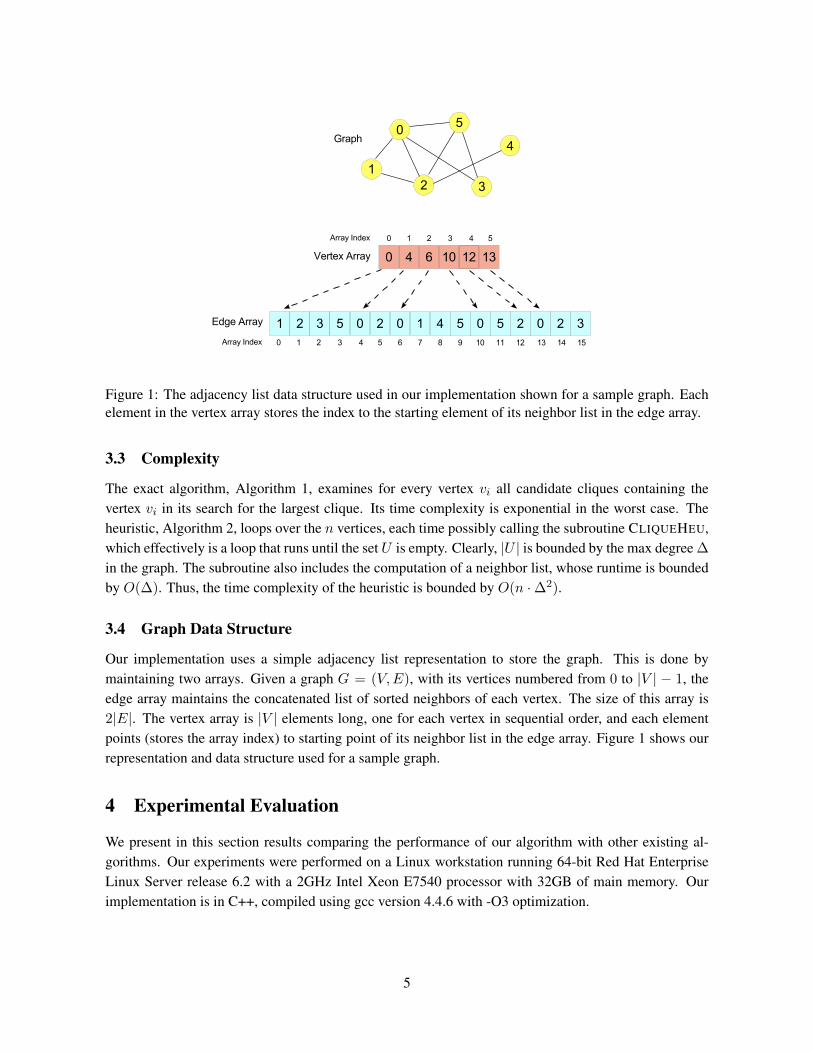
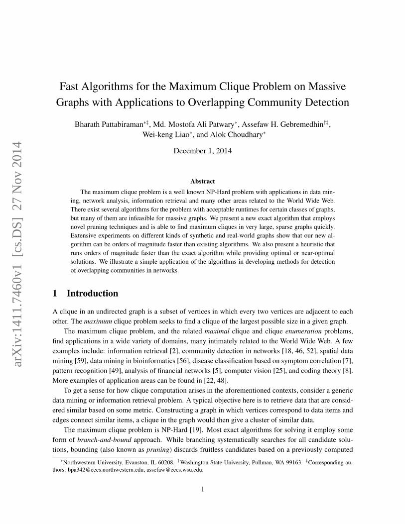
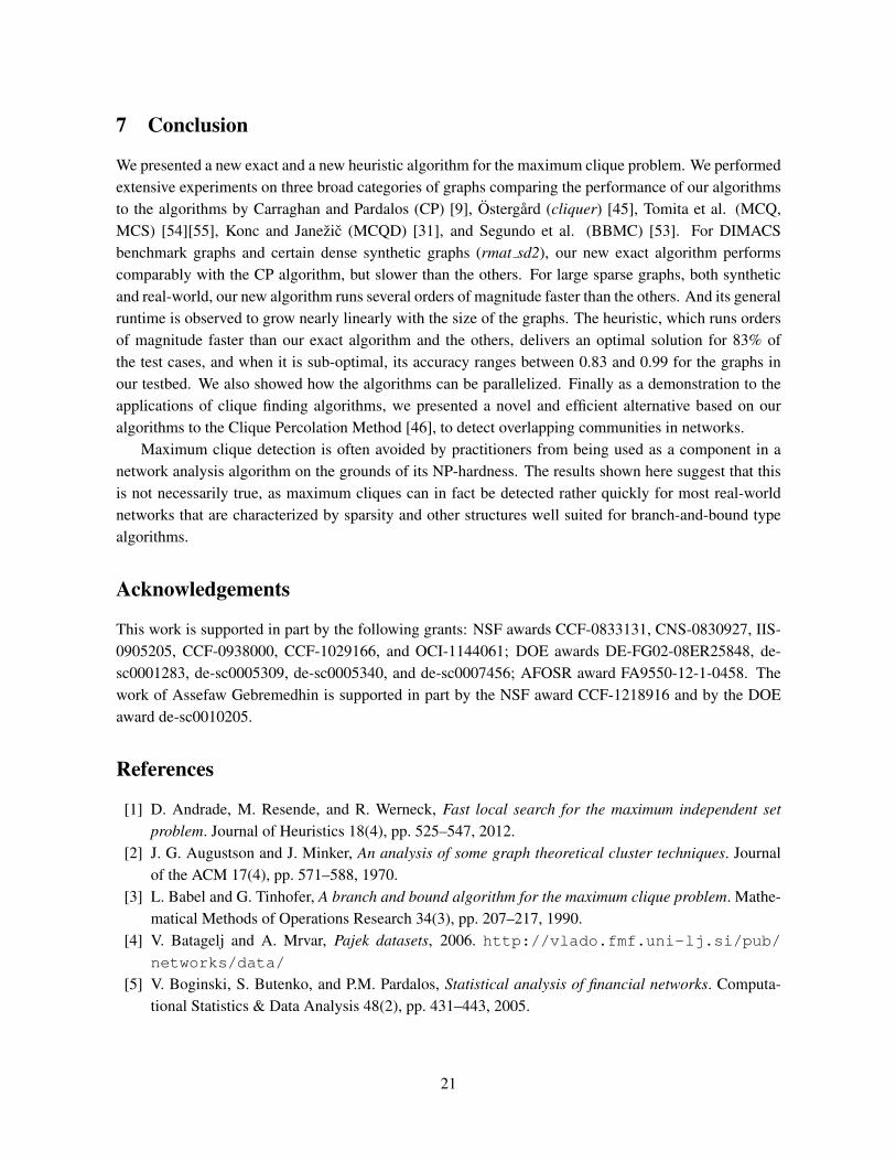
Figure 1: The adjacency list data structure used in our implementation shown for a sample graph. Eachelement in the vertex array stores the index to the starting element of its neighbor list in the edge array.

3.3 Complexity

The exact algorithm, Algorithm 1, examines for every vertex vi all candidate cliques containing thevertex vi in its search for the largest clique. Its time complexity is exponential in the worst case. Theheuristic, Algorithm 2, loops over the n vertices, each time possibly calling the subroutine CLIQUEHEU,which effectively is a loop that runs until the set U is empty. Clearly, |U | is bounded by the max degree ∆

in the graph. The subroutine also includes the computation of a neighbor list, whose runtime is boundedby O(∆). Thus, the time complexity of the heuristic is bounded by O(n ·∆2).

3.4 Graph Data Structure

Our implementation uses a simple adjacency list representation to store the graph. This is done bymaintaining two arrays. Given a graph G = (V,E), with its vertices numbered from 0 to |V | − 1, theedge array maintains the concatenated list of sorted neighbors of each vertex. The size of this array is2|E|. The vertex array is |V | elements long, one for each vertex in sequential order, and each elementpoints (stores the array index) to starting point of its neighbor list in the edge array. Figure 1 shows ourrepresentation and data structure used for a sample graph.

4 Experimental Evaluation

We present in this section results comparing the performance of our algorithm with other existing al-gorithms. Our experiments were performed on a Linux workstation running 64-bit Red Hat EnterpriseLinux Server release 6.2 with a 2GHz Intel Xeon E7540 processor with 32GB of main memory. Ourimplementation is in C++, compiled using gcc version 4.4.6 with -O3 optimization.

5

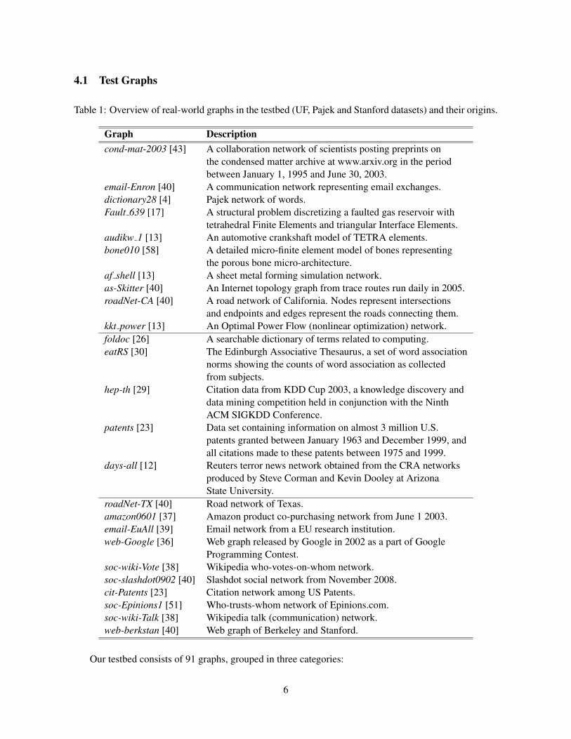
4.1 Test Graphs

Table 1: Overview of real-world graphs in the testbed (UF, Pajek and Stanford datasets) and their origins.

Graph Descriptioncond-mat-2003 [43] A collaboration network of scientists posting preprints on

the condensed matter archive at www.arxiv.org in the periodbetween January 1, 1995 and June 30, 2003.

email-Enron [40] A communication network representing email exchanges.dictionary28 [4] Pajek network of words.Fault 639 [17] A structural problem discretizing a faulted gas reservoir with

tetrahedral Finite Elements and triangular Interface Elements.audikw 1 [13] An automotive crankshaft model of TETRA elements.bone010 [58] A detailed micro-finite element model of bones representing

the porous bone micro-architecture.af shell [13] A sheet metal forming simulation network.as-Skitter [40] An Internet topology graph from trace routes run daily in 2005.roadNet-CA [40] A road network of California. Nodes represent intersections

and endpoints and edges represent the roads connecting them.kkt power [13] An Optimal Power Flow (nonlinear optimization) network.foldoc [26] A searchable dictionary of terms related to computing.eatRS [30] The Edinburgh Associative Thesaurus, a set of word association

norms showing the counts of word association as collectedfrom subjects.

hep-th [29] Citation data from KDD Cup 2003, a knowledge discovery anddata mining competition held in conjunction with the NinthACM SIGKDD Conference.

patents [23] Data set containing information on almost 3 million U.S.patents granted between January 1963 and December 1999, andall citations made to these patents between 1975 and 1999.

days-all [12] Reuters terror news network obtained from the CRA networksproduced by Steve Corman and Kevin Dooley at ArizonaState University.

roadNet-TX [40] Road network of Texas.amazon0601 [37] Amazon product co-purchasing network from June 1 2003.email-EuAll [39] Email network from a EU research institution.web-Google [36] Web graph released by Google in 2002 as a part of Google

Programming Contest.soc-wiki-Vote [38] Wikipedia who-votes-on-whom network.soc-slashdot0902 [40] Slashdot social network from November 2008.cit-Patents [23] Citation network among US Patents.soc-Epinions1 [51] Who-trusts-whom network of Epinions.com.soc-wiki-Talk [38] Wikipedia talk (communication) network.web-berkstan [40] Web graph of Berkeley and Stanford.

Our testbed consists of 91 graphs, grouped in three categories:

6

1) Real-world graphs. Under this category, we consider 10 graphs downloaded from the University ofFlorida (UF) Sparse Matrix Collection [13], 5 graphs from Pajek data sets [4], and 10 graphs from theStanford Large Network Dataset Collection [35]. The graphs originate from various real-world applica-tions. Table 1 gives a quick overview of the graphs and their origins.2) Synthetic Graphs. In this category we consider 15 graphs generated using the R-MAT algorithm

[10]. The graphs are subdivided in three categories depending on the structures they represent:a) Random graphs (5 graphs) – Erdos-Renyi random graphs generated using R-MAT with the parame-ters (0.25, 0.25, 0.25, 0.25). We denoted these with prefix rmat er.b) Skewed Degree, Type 1 graphs (5 graphs) – graphs generated using R-MAT with the parameters

(0.45, 0.15, 0.15, 0.25). These are denoted with prefix rmat sd1.c) Skewed Degree, Type 2 graphs (5 graphs) – graphs generated using R-MAT with the parameters

(0.55, 0.15, 0.15, 0.15). These are denoted with prefix rmat sd2.3) DIMACS graphs. This last category consists of 51 graphs selected from the Second DIMACS

Implementation Challenge [28]. Among these, 5 graphs are considered for discussion in the next fewsections, while the results for the rest are reported in Table 10 in the Appendix.

The DIMACS graphs are an established benchmark for the maximum clique problem, but they areof rather limited size and variation. In contrast, the real-work networks included in category 1 of thetestset and the synthetic (RMAT) graphs in category 2 represent a wide spectrum of large graphs posingvarying degrees of difficulty for the algorithms. The rmat er graphs have normal degree distribution,whereas the rmat sd1 and rmat sd2 graphs have skewed degree distributions and contain many denselocal subgraphs. The rmat sd1 and rmat sd2 graphs differ primarily in the magnitude of maximumvertex degree they contain; the rmat sd2 graphs have much higher maximum degree. Table 2 lists basicstructural information (the number of vertices, number of edges and the maximum degree) about 45 ofthe test graphs (25 real-world, 15 synthetic and 5 DIMACS).

4.2 Algorithms for Comparison

The algorithms we consider for comparison are the ones by:

• Carraghan-Pardalos [9]. We used our own implementation of this algorithm.

• Ostergard algorithm [45]. We used the publicly available cliquer source code [44].

• Konc and Janezic [31]. We used the code MaxCliqueDyn or MCQD, available athttp://www.sicmm.org/˜konc/maxclique/. Among the variants available in MCQD, wereport results on MCQD+CS (which uses improved coloring and dynamic sorting), since it is thebest-performing variant. The MaxCliqueDyn code was not capable of handling large input graphsand had to be aborted for many instances. For those that it successfully ran, we had to first modifythe graph reader to make it able to handle graphs with multiple connected components.

• Tomita and Seki (MCQ) [54].

• Tomita et al. (MCS) [55].

• San Segundo et al. (BBMC) [53].

For MCQ, MCS, and BBMC, we used the publicly available Java implementation, MCQ1, MCSa1, andBBMC1 respectively, by Prosser [50] available at http://www.dcs.gla.ac.uk/˜pat/maxClique/.

7

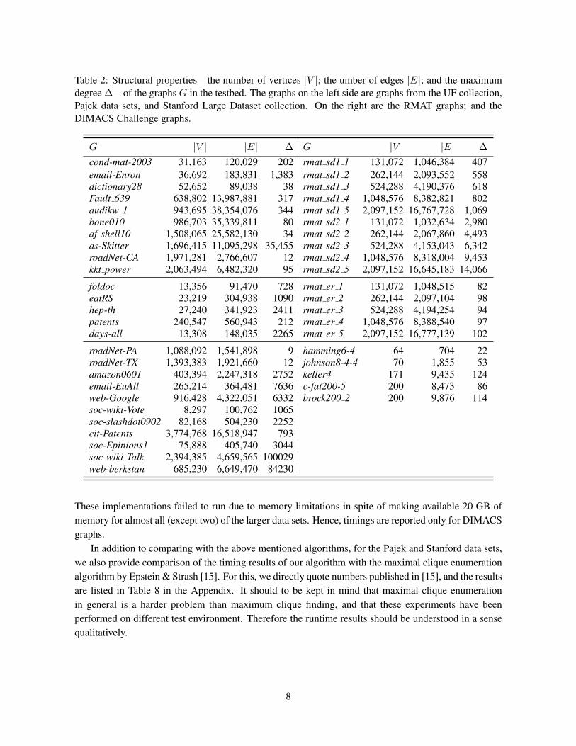
Table 2: Structural properties—the number of vertices |V |; the umber of edges |E|; and the maximumdegree ∆—of the graphs G in the testbed. The graphs on the left side are graphs from the UF collection,Pajek data sets, and Stanford Large Dataset collection. On the right are the RMAT graphs; and theDIMACS Challenge graphs.

G |V | |E| ∆ G |V | |E| ∆

cond-mat-2003 31,163 120,029 202 rmat sd1 1 131,072 1,046,384 407email-Enron 36,692 183,831 1,383 rmat sd1 2 262,144 2,093,552 558dictionary28 52,652 89,038 38 rmat sd1 3 524,288 4,190,376 618Fault 639 638,802 13,987,881 317 rmat sd1 4 1,048,576 8,382,821 802audikw 1 943,695 38,354,076 344 rmat sd1 5 2,097,152 16,767,728 1,069bone010 986,703 35,339,811 80 rmat sd2 1 131,072 1,032,634 2,980af shell10 1,508,065 25,582,130 34 rmat sd2 2 262,144 2,067,860 4,493as-Skitter 1,696,415 11,095,298 35,455 rmat sd2 3 524,288 4,153,043 6,342roadNet-CA 1,971,281 2,766,607 12 rmat sd2 4 1,048,576 8,318,004 9,453kkt power 2,063,494 6,482,320 95 rmat sd2 5 2,097,152 16,645,183 14,066

foldoc 13,356 91,470 728 rmat er 1 131,072 1,048,515 82eatRS 23,219 304,938 1090 rmat er 2 262,144 2,097,104 98hep-th 27,240 341,923 2411 rmat er 3 524,288 4,194,254 94patents 240,547 560,943 212 rmat er 4 1,048,576 8,388,540 97days-all 13,308 148,035 2265 rmat er 5 2,097,152 16,777,139 102

roadNet-PA 1,088,092 1,541,898 9 hamming6-4 64 704 22roadNet-TX 1,393,383 1,921,660 12 johnson8-4-4 70 1,855 53amazon0601 403,394 2,247,318 2752 keller4 171 9,435 124email-EuAll 265,214 364,481 7636 c-fat200-5 200 8,473 86web-Google 916,428 4,322,051 6332 brock200 2 200 9,876 114soc-wiki-Vote 8,297 100,762 1065soc-slashdot0902 82,168 504,230 2252cit-Patents 3,774,768 16,518,947 793soc-Epinions1 75,888 405,740 3044soc-wiki-Talk 2,394,385 4,659,565 100029web-berkstan 685,230 6,649,470 84230

These implementations failed to run due to memory limitations in spite of making available 20 GB ofmemory for almost all (except two) of the larger data sets. Hence, timings are reported only for DIMACSgraphs.

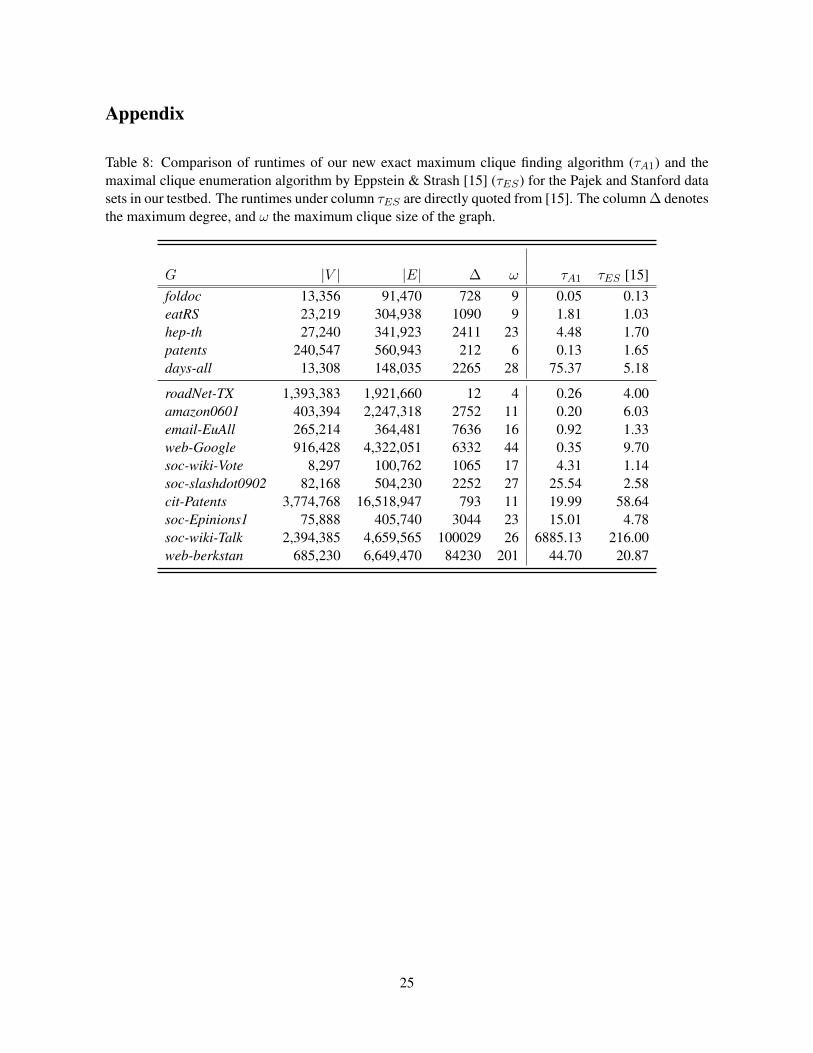
In addition to comparing with the above mentioned algorithms, for the Pajek and Stanford data sets,we also provide comparison of the timing results of our algorithm with the maximal clique enumerationalgorithm by Epstein & Strash [15]. For this, we directly quote numbers published in [15], and the resultsare listed in Table 8 in the Appendix. It should to be kept in mind that maximal clique enumerationin general is a harder problem than maximum clique finding, and that these experiments have beenperformed on different test environment. Therefore the runtime results should be understood in a sensequalitatively.

8

4.3 Results

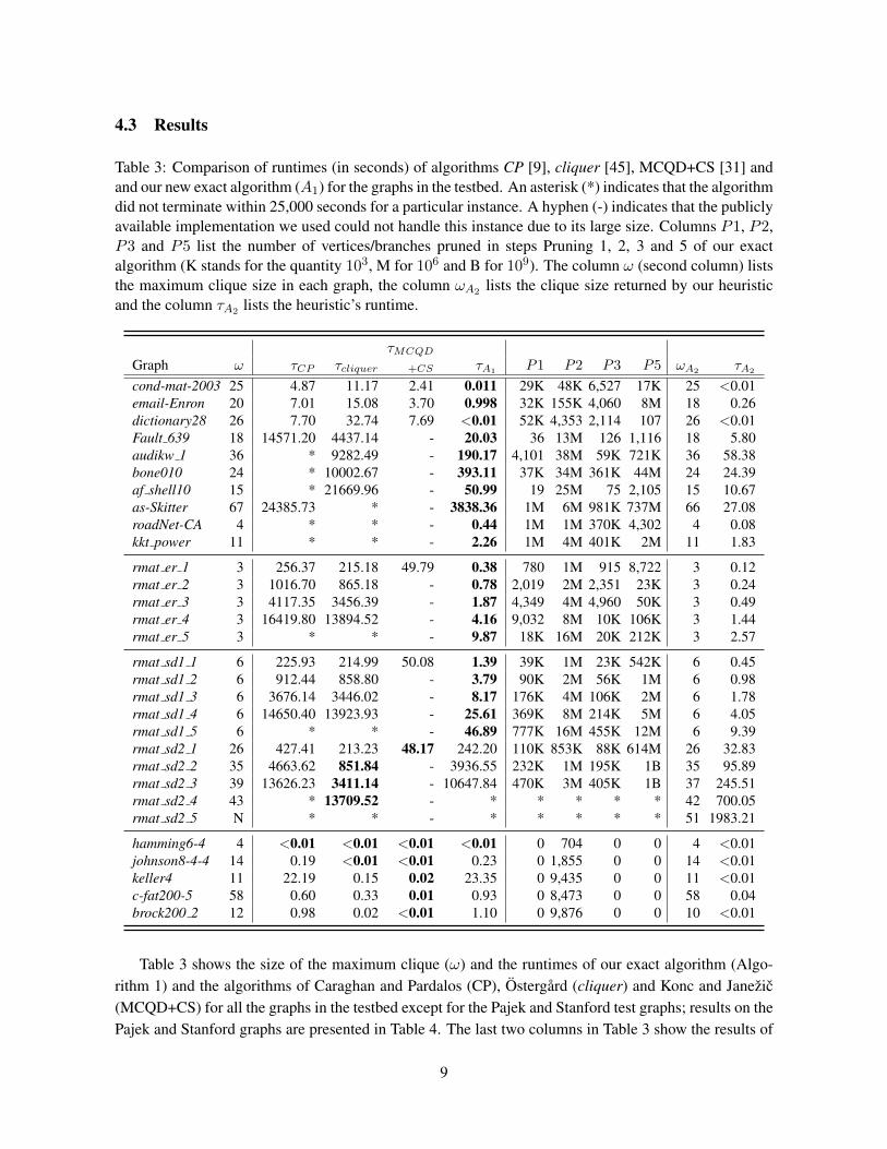
Table 3: Comparison of runtimes (in seconds) of algorithms CP [9], cliquer [45], MCQD+CS [31] andand our new exact algorithm (A1) for the graphs in the testbed. An asterisk (*) indicates that the algorithmdid not terminate within 25,000 seconds for a particular instance. A hyphen (-) indicates that the publiclyavailable implementation we used could not handle this instance due to its large size. Columns P1, P2,P3 and P5 list the number of vertices/branches pruned in steps Pruning 1, 2, 3 and 5 of our exactalgorithm (K stands for the quantity 103, M for 106 and B for 109). The column ω (second column) liststhe maximum clique size in each graph, the column ωA2 lists the clique size returned by our heuristicand the column τA2 lists the heuristic’s runtime.

τMCQD

Graph ω τCP τcliquer +CS τA1P1 P2 P3 P5 ωA2

τA2

cond-mat-2003 25 4.87 11.17 2.41 0.011 29K 48K 6,527 17K 25 <0.01email-Enron 20 7.01 15.08 3.70 0.998 32K 155K 4,060 8M 18 0.26dictionary28 26 7.70 32.74 7.69 <0.01 52K 4,353 2,114 107 26 <0.01Fault 639 18 14571.20 4437.14 - 20.03 36 13M 126 1,116 18 5.80audikw 1 36 * 9282.49 - 190.17 4,101 38M 59K 721K 36 58.38bone010 24 * 10002.67 - 393.11 37K 34M 361K 44M 24 24.39af shell10 15 * 21669.96 - 50.99 19 25M 75 2,105 15 10.67as-Skitter 67 24385.73 * - 3838.36 1M 6M 981K 737M 66 27.08roadNet-CA 4 * * - 0.44 1M 1M 370K 4,302 4 0.08kkt power 11 * * - 2.26 1M 4M 401K 2M 11 1.83

rmat er 1 3 256.37 215.18 49.79 0.38 780 1M 915 8,722 3 0.12rmat er 2 3 1016.70 865.18 - 0.78 2,019 2M 2,351 23K 3 0.24rmat er 3 3 4117.35 3456.39 - 1.87 4,349 4M 4,960 50K 3 0.49rmat er 4 3 16419.80 13894.52 - 4.16 9,032 8M 10K 106K 3 1.44rmat er 5 3 * * - 9.87 18K 16M 20K 212K 3 2.57

rmat sd1 1 6 225.93 214.99 50.08 1.39 39K 1M 23K 542K 6 0.45rmat sd1 2 6 912.44 858.80 - 3.79 90K 2M 56K 1M 6 0.98rmat sd1 3 6 3676.14 3446.02 - 8.17 176K 4M 106K 2M 6 1.78rmat sd1 4 6 14650.40 13923.93 - 25.61 369K 8M 214K 5M 6 4.05rmat sd1 5 6 * * - 46.89 777K 16M 455K 12M 6 9.39rmat sd2 1 26 427.41 213.23 48.17 242.20 110K 853K 88K 614M 26 32.83rmat sd2 2 35 4663.62 851.84 - 3936.55 232K 1M 195K 1B 35 95.89rmat sd2 3 39 13626.23 3411.14 - 10647.84 470K 3M 405K 1B 37 245.51rmat sd2 4 43 * 13709.52 - * * * * * 42 700.05rmat sd2 5 N * * - * * * * * 51 1983.21

hamming6-4 4 <0.01 <0.01 <0.01 <0.01 0 704 0 0 4 <0.01johnson8-4-4 14 0.19 <0.01 <0.01 0.23 0 1,855 0 0 14 <0.01keller4 11 22.19 0.15 0.02 23.35 0 9,435 0 0 11 <0.01c-fat200-5 58 0.60 0.33 0.01 0.93 0 8,473 0 0 58 0.04brock200 2 12 0.98 0.02 <0.01 1.10 0 9,876 0 0 10 <0.01

Table 3 shows the size of the maximum clique (ω) and the runtimes of our exact algorithm (Algo-rithm 1) and the algorithms of Caraghan and Pardalos (CP), Ostergard (cliquer) and Konc and Janezic(MCQD+CS) for all the graphs in the testbed except for the Pajek and Stanford test graphs; results on thePajek and Stanford graphs are presented in Table 4. The last two columns in Table 3 show the results of

9

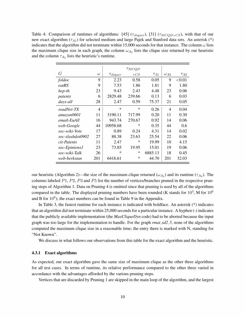
Table 4: Comparison of runtimes of algorithms: [45] (τcliquer), [31] (τMCQD+CS), with that of ournew exact algorithm (τA1) for selected medium and large Pajek and Stanford data sets. An asterisk (*)indicates that the algorithm did not terminate within 15,000 seconds for that instance. The column ω liststhe maximum clique size in each graph, the column ωA2 lists the clique size returned by our heuristicand the column τA2 lists the heuristic’s runtime.

τMCQD

G ω τcliquer +CS τA1 ωA2 τA2

foldoc 9 2.23 0.58 0.05 9 <0.01eatRS 9 7.53 1.86 1.81 9 1.80hep-th 23 9.43 2.43 4.48 23 0.06patents 6 2829.48 239.66 0.13 6 0.03days-all 28 2.47 0.59 75.37 21 0.05

roadNet-TX 4 * * 0.26 4 0.04amazon0601 11 3190.11 717.99 0.20 11 0.30email-EuAll 16 943.74 270.67 0.92 14 0.06web-Google 44 10958.68 * 0.35 44 0.6soc-wiki-Vote 17 0.89 0.24 4.31 14 0.02soc-slashdot0902 27 88.38 23.63 25.54 22 0.06cit-Patents 11 2.47 * 19.99 10 4.15soc-Epinions1 23 73.85 19.95 15.01 19 0.06soc-wiki-Talk 26 * * 6885.13 18 0.45web-berkstan 201 6416.61 * 44.70 201 32.03

our heuristic (Algorithm 2)—the size of the maximum clique returned (ωA2) and its runtime (τA2). Thecolumns labeled P1, P2, P3 and P5 list the number of vertices/branches pruned in the respective prun-ing steps of Algorithm 1. Data on Pruning 4 is omitted since that pruning is used by all of the algorithmscompared in the table. The displayed pruning numbers have been rounded (K stands for 103, M for 106

and B for 109); the exact numbers can be found in Table 9 in the Appendix.In Table 3, the fastest runtime for each instance is indicated with boldface. An asterisk (*) indicates

that an algorithm did not terminate within 25,000 seconds for a particular instance. A hyphen (-) indicatesthat the publicly available implementation (the MaxCliqueDyn code) had to be aborted because the inputgraph was too large for the implementation to handle. For the graph rmat sd2 5, none of the algorithmscomputed the maximum clique size in a reasonable time; the entry there is marked with N, standing for“Not Known”.

We discuss in what follows our observations from this table for the exact algorithm and the heuristic.

4.3.1 Exact algorithms

As expected, our exact algorithm gave the same size of maximum clique as the other three algorithmsfor all test cases. In terms of runtime, its relative performance compared to the other three varied inaccordance with the advantages afforded by the various pruning steps.

Vertices that are discarded by Pruning 1 are skipped in the main loop of the algorithm, and the largest

10

0

20

40

60

80

100

120

140

cond-­‐mat-­‐2003

email-­‐Enron

dic6onary28

Fault_639

audikw_1

bone010

af_shell10

as-­‐SkiCer

roadNet-­‐CA

kkt_power

Normalized

prune

d ver0ces (%)

P1 P2 P3 P4 P5

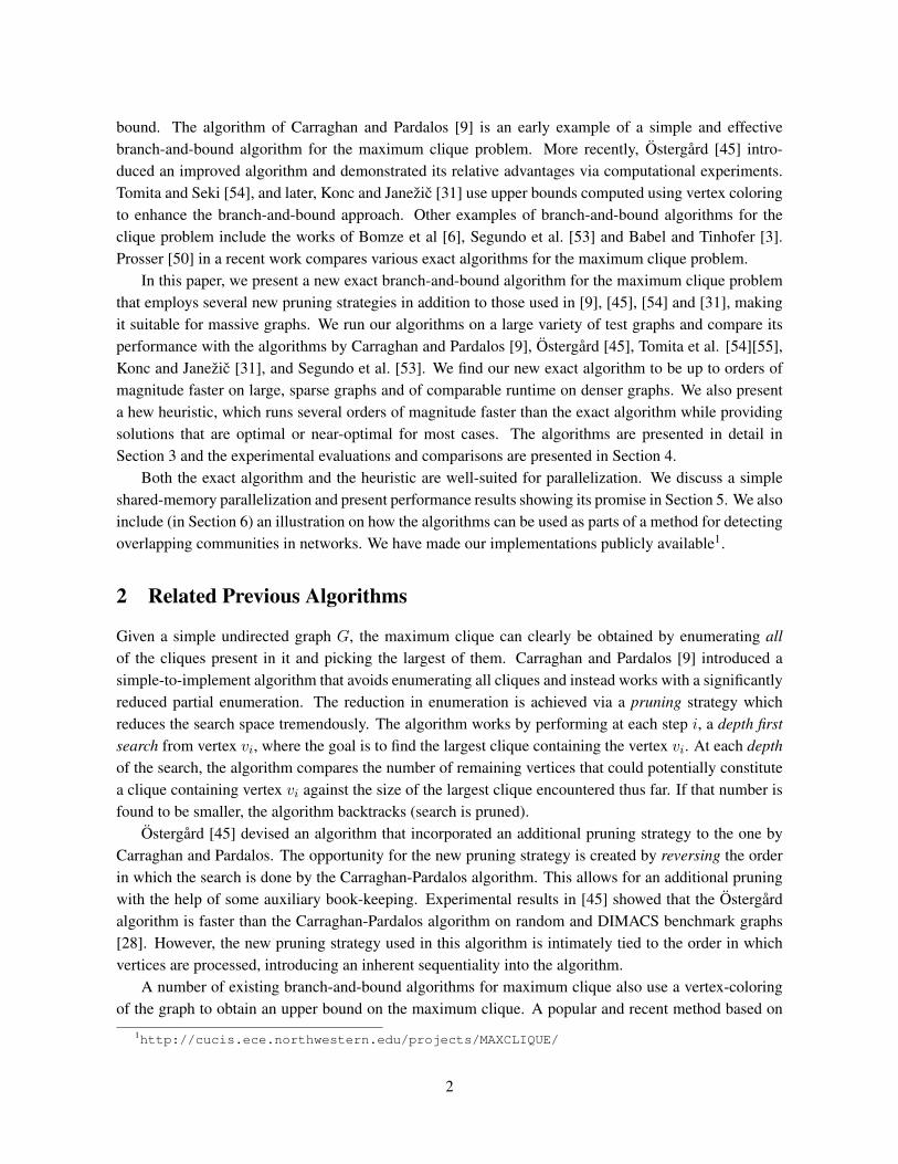
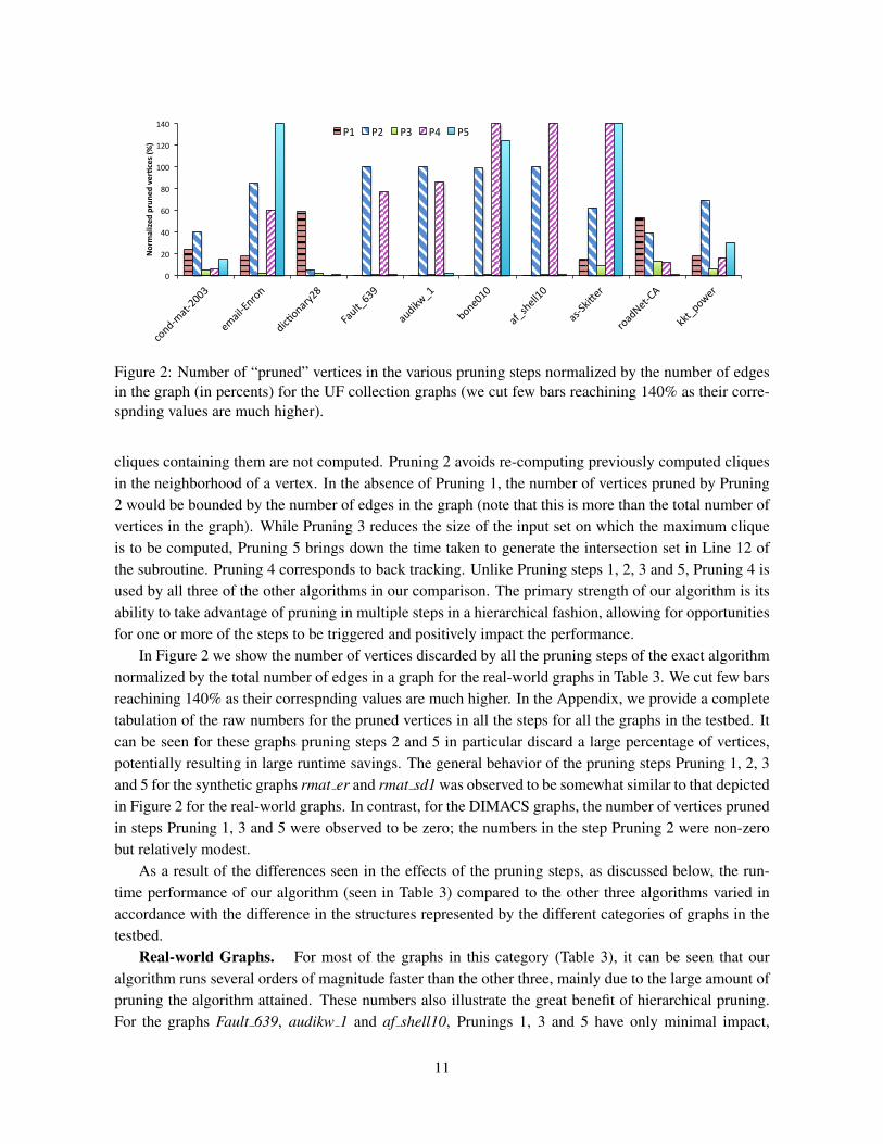
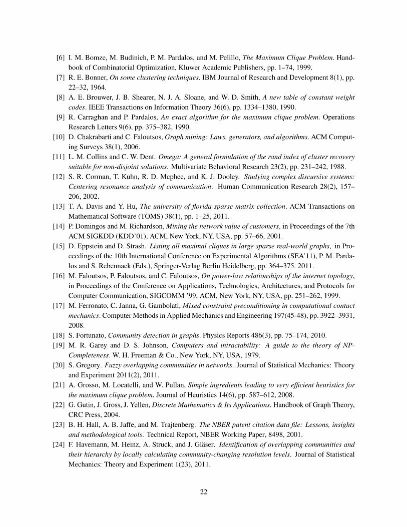
Figure 2: Number of “pruned” vertices in the various pruning steps normalized by the number of edgesin the graph (in percents) for the UF collection graphs (we cut few bars reachining 140% as their corre-spnding values are much higher).

cliques containing them are not computed. Pruning 2 avoids re-computing previously computed cliquesin the neighborhood of a vertex. In the absence of Pruning 1, the number of vertices pruned by Pruning2 would be bounded by the number of edges in the graph (note that this is more than the total number ofvertices in the graph). While Pruning 3 reduces the size of the input set on which the maximum cliqueis to be computed, Pruning 5 brings down the time taken to generate the intersection set in Line 12 ofthe subroutine. Pruning 4 corresponds to back tracking. Unlike Pruning steps 1, 2, 3 and 5, Pruning 4 isused by all three of the other algorithms in our comparison. The primary strength of our algorithm is itsability to take advantage of pruning in multiple steps in a hierarchical fashion, allowing for opportunitiesfor one or more of the steps to be triggered and positively impact the performance.

In Figure 2 we show the number of vertices discarded by all the pruning steps of the exact algorithmnormalized by the total number of edges in a graph for the real-world graphs in Table 3. We cut few barsreachining 140% as their correspnding values are much higher. In the Appendix, we provide a completetabulation of the raw numbers for the pruned vertices in all the steps for all the graphs in the testbed. Itcan be seen for these graphs pruning steps 2 and 5 in particular discard a large percentage of vertices,potentially resulting in large runtime savings. The general behavior of the pruning steps Pruning 1, 2, 3and 5 for the synthetic graphs rmat er and rmat sd1 was observed to be somewhat similar to that depictedin Figure 2 for the real-world graphs. In contrast, for the DIMACS graphs, the number of vertices prunedin steps Pruning 1, 3 and 5 were observed to be zero; the numbers in the step Pruning 2 were non-zerobut relatively modest.

As a result of the differences seen in the effects of the pruning steps, as discussed below, the run-time performance of our algorithm (seen in Table 3) compared to the other three algorithms varied inaccordance with the difference in the structures represented by the different categories of graphs in thetestbed.

Real-world Graphs. For most of the graphs in this category (Table 3), it can be seen that ouralgorithm runs several orders of magnitude faster than the other three, mainly due to the large amount ofpruning the algorithm attained. These numbers also illustrate the great benefit of hierarchical pruning.For the graphs Fault 639, audikw 1 and af shell10, Prunings 1, 3 and 5 have only minimal impact,

11

0

0.5

1

real-­‐world rmat_er rmat_sd1 rmat_sd2 DIMACS

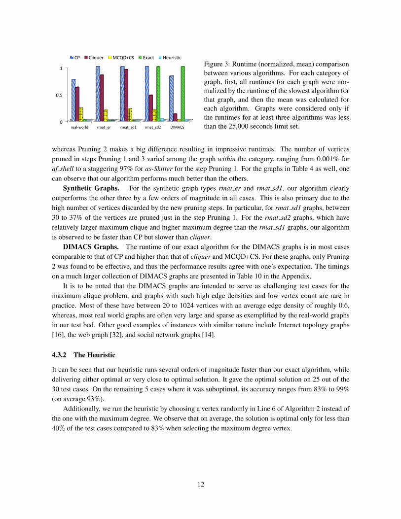
CP Cliquer MCQD+CS Exact HeurisCc Figure 3: Runtime (normalized, mean) comparisonbetween various algorithms. For each category ofgraph, first, all runtimes for each graph were nor-malized by the runtime of the slowest algorithm forthat graph, and then the mean was calculated foreach algorithm. Graphs were considered only ifthe runtimes for at least three algorithms was lessthan the 25,000 seconds limit set.

whereas Pruning 2 makes a big difference resulting in impressive runtimes. The number of verticespruned in steps Pruning 1 and 3 varied among the graph within the category, ranging from 0.001% foraf shell to a staggering 97% for as-Skitter for the step Pruning 1. For the graphs in Table 4 as well, onecan observe that our algorithm performs much better than the others.

Synthetic Graphs. For the synthetic graph types rmat er and rmat sd1, our algorithm clearlyoutperforms the other three by a few orders of magnitude in all cases. This is also primary due to thehigh number of vertices discarded by the new pruning steps. In particular, for rmat sd1 graphs, between30 to 37% of the vertices are pruned just in the step Pruning 1. For the rmat sd2 graphs, which haverelatively larger maximum clique and higher maximum degree than the rmat sd1 graphs, our algorithmis observed to be faster than CP but slower than cliquer.

DIMACS Graphs. The runtime of our exact algorithm for the DIMACS graphs is in most casescomparable to that of CP and higher than that of cliquer and MCQD+CS. For these graphs, only Pruning2 was found to be effective, and thus the performance results agree with one’s expectation. The timingson a much larger collection of DIMACS graphs are presented in Table 10 in the Appendix.

It is to be noted that the DIMACS graphs are intended to serve as challenging test cases for themaximum clique problem, and graphs with such high edge densities and low vertex count are rare inpractice. Most of these have between 20 to 1024 vertices with an average edge density of roughly 0.6,whereas, most real world graphs are often very large and sparse as exemplified by the real-world graphsin our test bed. Other good examples of instances with similar nature include Internet topology graphs[16], the web graph [32], and social network graphs [14].

4.3.2 The Heuristic

It can be seen that our heuristic runs several orders of magnitude faster than our exact algorithm, whiledelivering either optimal or very close to optimal solution. It gave the optimal solution on 25 out of the30 test cases. On the remaining 5 cases where it was suboptimal, its accuracy ranges from 83% to 99%(on average 93%).

Additionally, we run the heuristic by choosing a vertex randomly in Line 6 of Algorithm 2 instead ofthe one with the maximum degree. We observe that on average, the solution is optimal only for less than40% of the test cases compared to 83% when selecting the maximum degree vertex.

12

0.00

0.00

0.01

0.10

1.00

10.00

rmat_er_1

rmat_er_2

rmat_er_3

rmat_er_4

rmat_er_5

Time (sec) in log-­‐scale

exact heuris5c edges

0.00

0.00

0.01

0.10

1.00

10.00

100.00

rmat_sd1_1

rmat_sd1_2

rmat_sd1_3

rmat_sd1_4

rmat_sd1_5

Time (sec) in log-­‐scale

exact heuris6c edges

1.E-­‐04 1.E-­‐03 1.E-­‐02 1.E-­‐01 1.E+00 1.E+01 1.E+02 1.E+03 1.E+04 1.E+05

rmat_sd2_1

rmat_sd2_2

rmat_sd2_3

rmat_sd2_4

rmat_sd2_5

Time (sec) in log-­‐scale

exact heuris9c edges

1.E-­‐05 1.E-­‐04 1.E-­‐03 1.E-­‐02 1.E-­‐01 1.E+00 1.E+01 1.E+02 1.E+03 1.E+04

dic/onary28

cond-­‐mat-­‐2003

roadNet-­‐CA

email-­‐Enron

kkt_power

Fault_639

af_shell10

audikw_1

bone010

as-­‐SkiJer

Time (sec) in log-­‐scale

exact heuris/c edges

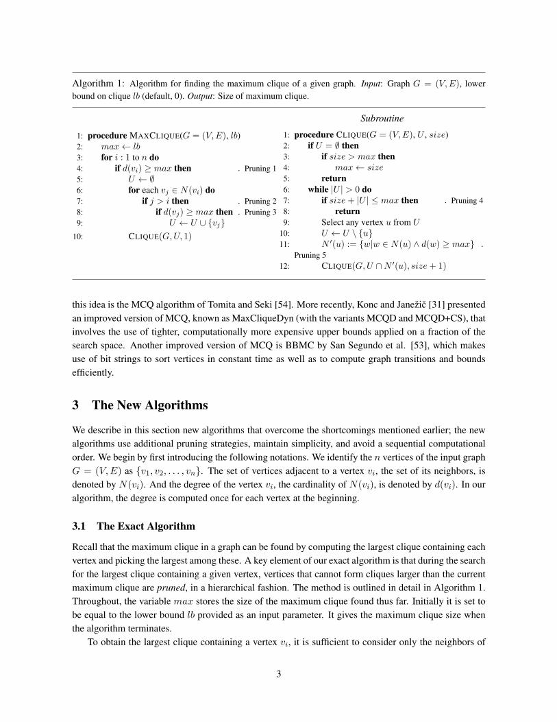
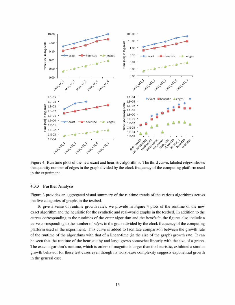
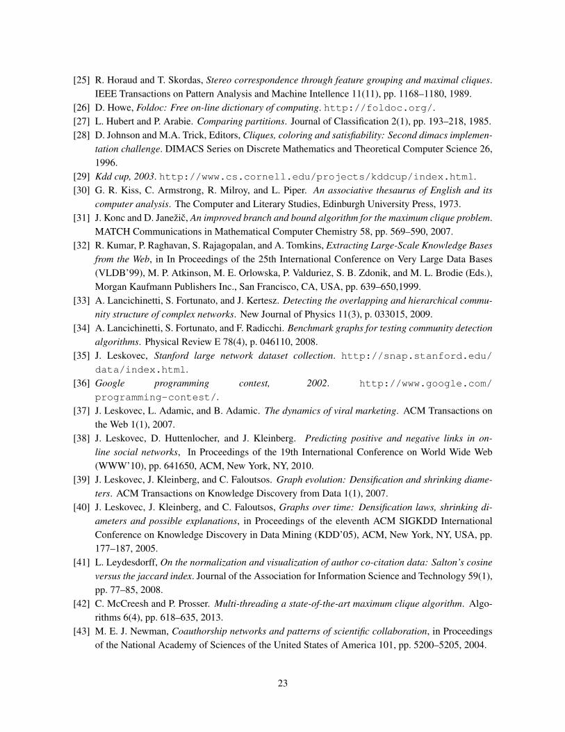
Figure 4: Run time plots of the new exact and heuristic algorithms. The third curve, labeled edges, showsthe quantity number of edges in the graph divided by the clock frequency of the computing platform usedin the experiment.

4.3.3 Further Analysis

Figure 3 provides an aggregated visual summary of the runtime trends of the various algorithms acrossthe five categories of graphs in the testbed.

To give a sense of runtime growth rates, we provide in Figure 4 plots of the runtime of the newexact algorithm and the heuristic for the synthetic and real-world graphs in the testbed. In addition to thecurves corresponding to the runtimes of the exact algorithm and the heuristic, the figures also include acurve corresponding to the number of edges in the graph divided by the clock frequency of the computingplatform used in the experiment. This curve is added to facilitate comparison between the growth rateof the runtime of the algorithms with that of a linear-time (in the size of the graph) growth rate. It canbe seen that the runtime of the heuristic by and large grows somewhat linearly with the size of a graph.The exact algorithm’s runtime, which is orders of magnitude larger than the heuristic, exhibited a similargrowth behavior for these test-cases even though its worst-case complexity suggests exponential growthin the general case.

13

5 Parallelization

We demonstrate in this section how our exact algorithm can be parallelized and show performance resultson a shared-memory platform. The heuristic can be parallelized following a similar procedure.

As explained in Section 3, the ith iteration of the for loop in the exact algorithm (Algorithm 1) com-putes the size of the largest clique that contains the vertex vi. Since our algorithm does not imposeany specific order in which vertices have to be processed, these iterations can in principle be performedconcurrently. During such a concurrent computation, however, different processes might discover max-imum cliques of different sizes—and for the pruning steps to be most effective, the current globallylargest maximum clique size needs to be communicated to all processes as soon as it is discovered. In ashared-memory programming model, the global maximum clique size can be stored as a shared variableaccessible to all the processing units, and its value can be updated by the relevant processor at any giventime. In a distributed-memory setting, more care needs to be exercised to keep the communication costlow.

We implemented a shared-memory parallelization based on the procedure described above usingOpenMP. Since the global value of the maximum clique is shared by all processing units, we embed thestep that updates the maximum clique, i.e. Line 4 of Algorithm 1, into a critical section (an OpenMPfeature that enforces a lock, thus allowing only one thread at a time to make the update). Further, weuse dynamic load scheduling, since different vertices might return different sizes of maximum cliqueresulting in different work loads.

We performed experiments on the same graphs listed in the testbed described in Section 4. For these,we used a Linux workstation with six 2.00GHz Intel Xeon E7540 processors. Each processor has sixcores, each with 32KB of L1 and 256KB of L2 cache, and each processor shares an 18MB L3 cache.

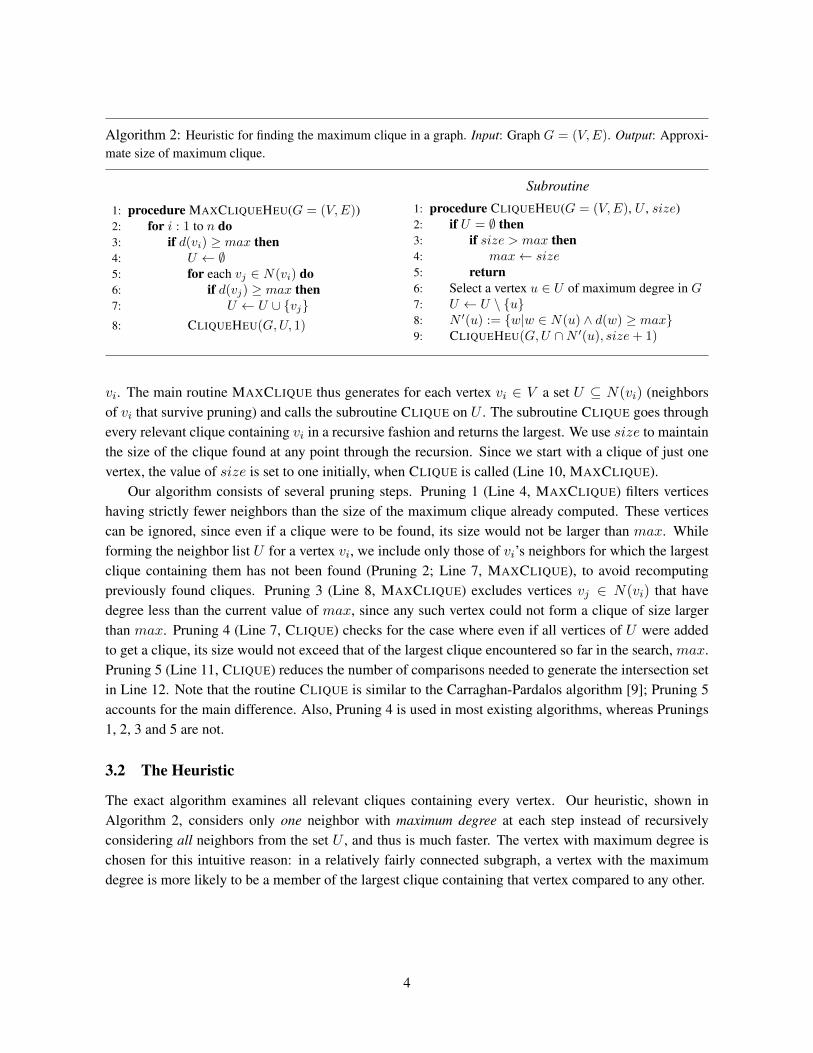
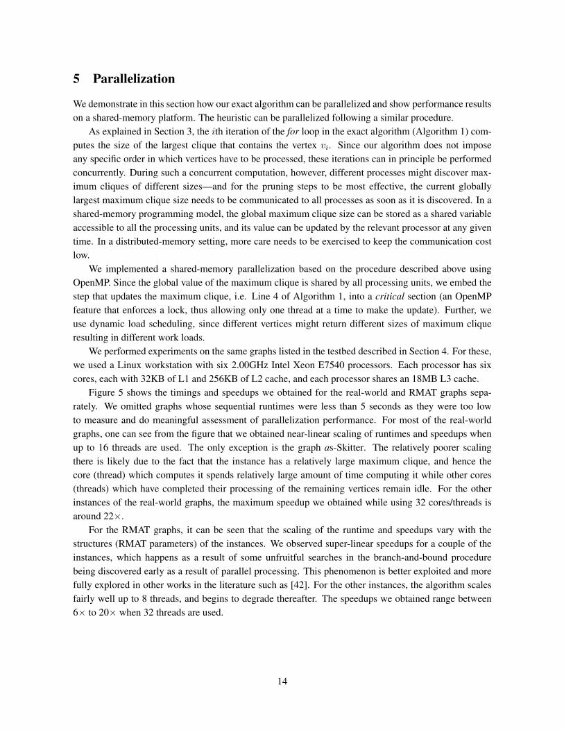
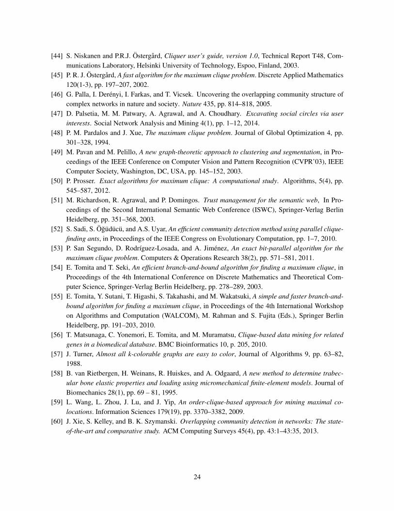
Figure 5 shows the timings and speedups we obtained for the real-world and RMAT graphs sepa-rately. We omitted graphs whose sequential runtimes were less than 5 seconds as they were too lowto measure and do meaningful assessment of parallelization performance. For most of the real-worldgraphs, one can see from the figure that we obtained near-linear scaling of runtimes and speedups whenup to 16 threads are used. The only exception is the graph as-Skitter. The relatively poorer scalingthere is likely due to the fact that the instance has a relatively large maximum clique, and hence thecore (thread) which computes it spends relatively large amount of time computing it while other cores(threads) which have completed their processing of the remaining vertices remain idle. For the otherinstances of the real-world graphs, the maximum speedup we obtained while using 32 cores/threads isaround 22×.

For the RMAT graphs, it can be seen that the scaling of the runtime and speedups vary with thestructures (RMAT parameters) of the instances. We observed super-linear speedups for a couple of theinstances, which happens as a result of some unfruitful searches in the branch-and-bound procedurebeing discovered early as a result of parallel processing. This phenomenon is better exploited and morefully explored in other works in the literature such as [42]. For the other instances, the algorithm scalesfairly well up to 8 threads, and begins to degrade thereafter. The speedups we obtained range between6× to 20× when 32 threads are used.

14

0.50 1.00 2.00 4.00 8.00

16.00 32.00 64.00 128.00 256.00 512.00 1024.00 2048.00 4096.00

1 2 4 8 16 32 Ru

n$me (in

second

s)

No. of threads

1

2

4

8

16

32

1 2 4 8 16 32

Speedu

p

No. of threads

Fault_639 audikw_1 bone010 af_shell10 as-­‐Ski=er Ideal

0.50 1.00 2.00 4.00 8.00

16.00 32.00 64.00 128.00 256.00 512.00 1024.00 2048.00 4096.00 8192.00

16384.00 1 2 4 8 16 32

Run$

me (in

second

s)

No. of threads

1.00

2.00

4.00

8.00

16.00

32.00

1 2 4 8 16 32

Speedu

p

No. of threads

rmat_er_5

rmat_sd1_3

rmat_sd1_4

rmat_sd1_5

rmat_sd2_1

rmat_sd2_2

rmat_sd2_3

Ideal

Figure 5: Performance (timing and speedup plots) of shared-memory parallelization on graphs in thetest-bed. The top set of figures show performance on the real-world graphs, whereas the bottom set showresults for the RMAT graphs. Graphs whose sequential runtime is less than 5 seconds were omitted.

6 Clique Algorithms and Community Detection

In this section we demonstrate how clique finding algorithms can be used for detecting overlappingcommunities in networks.

Background. Most community detection algorithms are designed to identify mutually independentcommunities in a given network and therefore are not suitable for detecting overlapping communities.Yet, in many real-world networks, it is natural to find vertices (or members) that belong to more than onegroup (or community) at the same time.

Palla et al. [46] introduced the Clique Percolation Method (CPM) as one effective approach fordetecting overlapping communities in a network. The basic premise in CPM is that a typical communityis likely to be made up of several cliques that share many of their vertices. We recall a few notionsdefined in [46] to make this more precise. A clique of size k is called a k-clique, and two k-cliques arecalled adjacent if they share k − 1 nodes. A k-clique community is a union of all k-cliques that can be

15

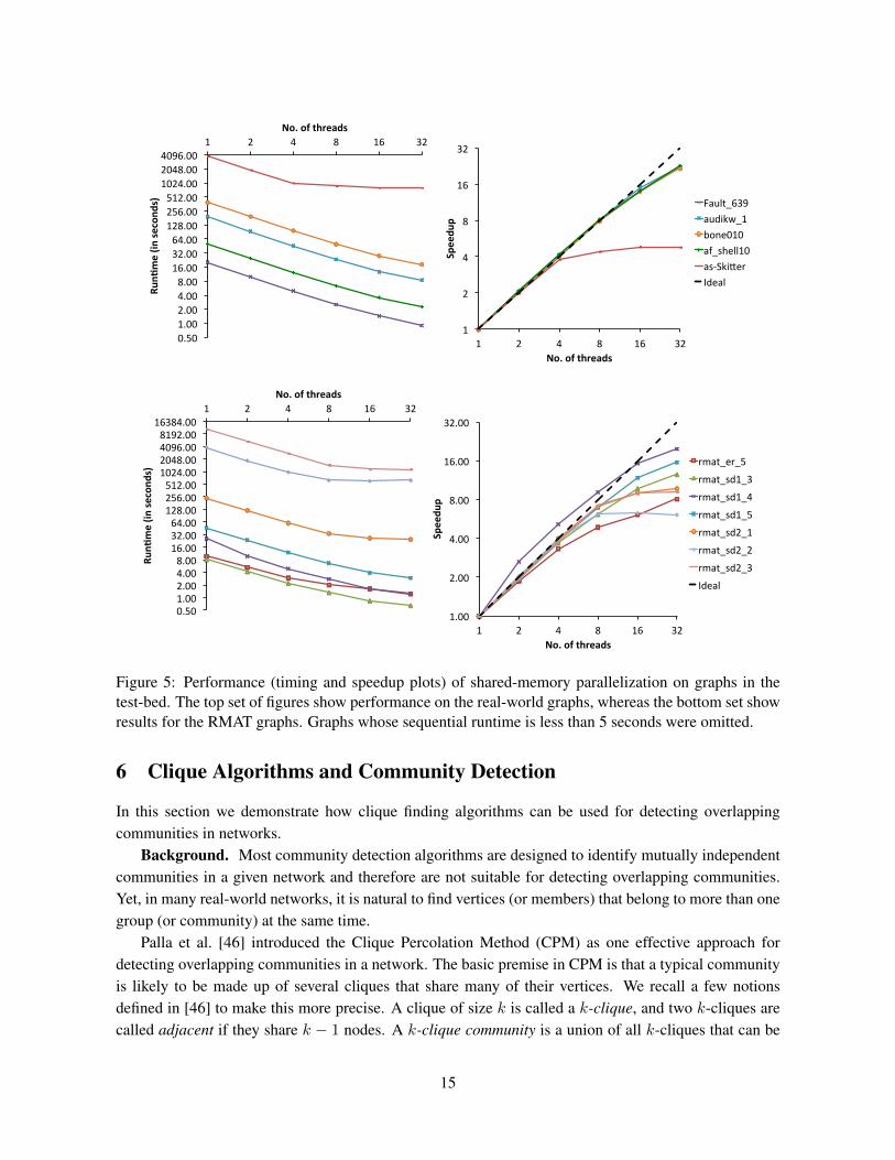
Figure 6: Illustration of overlapping community detection by the Clique Percolation Method (CPM) al-gorithm on a sample graph. Steps involved are 1) Detecting the k-cliques 2) Forming the clique-graph 3)Merging members of the connected components in the clique-graph to obtain the k-clique communities.In this example, node 2 is shared by the two communities formed, resulting in an overlapping structure.

reached from each other through a series of adjacent k-cliques. With these notions at hand, Palla et al.devise a method to extract such k-clique communities of a network. Note that, by definition, k-cliquecommunities allow for overlaps, i.e. common vertices can be shared by the communities.

The CPM algorithm is illustrated in Figure 6. Given a graph, we first extract all cliques of size k; forthis example we choose k=3. This is followed by generating the clique graph, where each k-clique inthe original graph is represented by a vertex. An edge is added between any two k-cliques in the cliquegraph that are adjacent. For the case k=3, this means an edge is added between any two 3-cliques in theclique graph that share two common vertices (of the original graph). The connected components in theclique graph represent a community, and the actual members of the community are obtained by gatheringthe vertices of the individual cliques that form the connected component. In our example in Figure 6, weobtain two communities, which share a common vertex (vertex 2), forming an overlapping communitystructure.

A large clique of size q ≥ k contains(qk

)different k-cliques. An algorithm that tries to locate the

k-cliques individually and examine the adjacency between them can therefore be very very slow for largenetworks. Palla et al. make two observations that help one come up with a better strategy. First, a cliqueof size q is clearly a k-clique connected subset for any k ≤ q. Second, two large cliques that share at leastk−1 nodes form one k-clique connected component as well. Leveraging these, the strategy of Palla et al.avoids searching for k-cliques individually and instead first locates the large cliques in the network and

16

then looks for the k-clique connected subsets of given k (that is, the k-clique communities) by studyingthe overlap between them. More specifically, their algorithm first constructs a symmetric clique-cliqueoverlap matrix, in which each row represents a large (to be precise a maximal) clique, each matrix entryis equal to the number of common nodes between the two corresponding cliques, and each diagonal entryis equal to the size of the clique. The k-clique communities for a given k are then equivalent to connectedclique components in which the neighboring cliques are linked to each other by at least k − 1 commonnodes. Palla et al. then find these components by erasing every off-diagonal entry smaller than k − 1

and every diagonal entry smaller than k in the matrix, replacing the remaining elements by one, and thencarrying out a component analysis of this matrix. The resulting separate components are equivalent tothe different k-clique communities.

Our Method. We devised an algorithm based on a similar idea as the procedure above, but using avariant of our heuristic maximum clique-algorithm (Algorithm 2) for the core clique detection step.

The standard CPM in essence presupposes finding all maximal cliques in a network. The number ofmaximal cliques in a network can in general be exponential in the number of nodes n in the network. Inour method, we work instead with a smaller set of maximal cliques. In particular, the basic variant ofour method considers exactly one clique per vertex, the largest of all the maximal cliques that it belongsto. Clearly, this can be too restrictive a requirement and may fail to add deserving members to a k-clique community. To allow for more refined solutions, we include a parameter c in the method thattells us how many additional cliques per vertex would be considered. The case c = 0 corresponds to noadditional cliques than the largest maximal clique containing the vertex. The case c ≥ 1 correspondsto c additional maximal cliques (each of size at least k) per vertex. Hence, in total, n(c + 1) cliqueswill be collected. For a particular vertex v, the largest maximal clique containing it can be heuristicallyobtained by exploring the neighbor of v with maximum degree in the corresponding step in Algorithm 2.In contrast, to obtain the other maximal cliques involving v (case c ≥ 1), we explore a randomly chosenneighbor of v, regardless of its degree value.

Test on Synthetic Networks. We tested our algorithm on the LFR benchmarks2 proposed in [34].These benchmarks have the attractive feature that they allow for generation of synthetic networks withknown communities (ground truth). We generated graphs with n = 1000 nodes, average degree K = 10,and power law exponents τ1 = 2 and τ2 = 1 in the LFR model. We set the maximum degree Kmax to50, and the minimum and maximum community sizes Cmin and Cmax to 20 and 50, respectively. Weused two far-apart values each for the mixing parameter µ, the fraction of overlapping nodes On, andthe number of communities each overlapping node belongs to Om. Specifically, for µ we used 0.1 and0.3, for On we used 10% and 50%, and for Om we used 2 and 8. All together, these combinations ofparameters resulted in eight graphs in the testbed.

We evaluated the performance of our algorithm against the ground truth using Omega Index [11],which is the overlapping version of the Adjusted Rand Index (ARI) [27]. Intuitively, Omega Indexmeasures the extent of agreement between two given sets of communities, by looking at node pairs thatoccur the same number of times (possibly none) in both. We used three values for the parameter c of ourmethod: 0, 2, and 5. Recall that c set to zero corresponds to picking only the largest clique for each node.As c is increased, more and more large cliques (each of size at least k) are considered for each node.

2http://sites.google.com/site/andrealancichinetti/files

17

We compare the performance of our method with that of CFinder3, an implementation of CPM [46]. Weused the command line utility provided in the package for all experiments. For this study, we used aMacBook Pro running OS X v.10.9.2 with 2.66GHz Intel Core i7 processor with 2 cores, 256KB of L2cache per core, 4MB of L3 cache and 8GB of main memory.

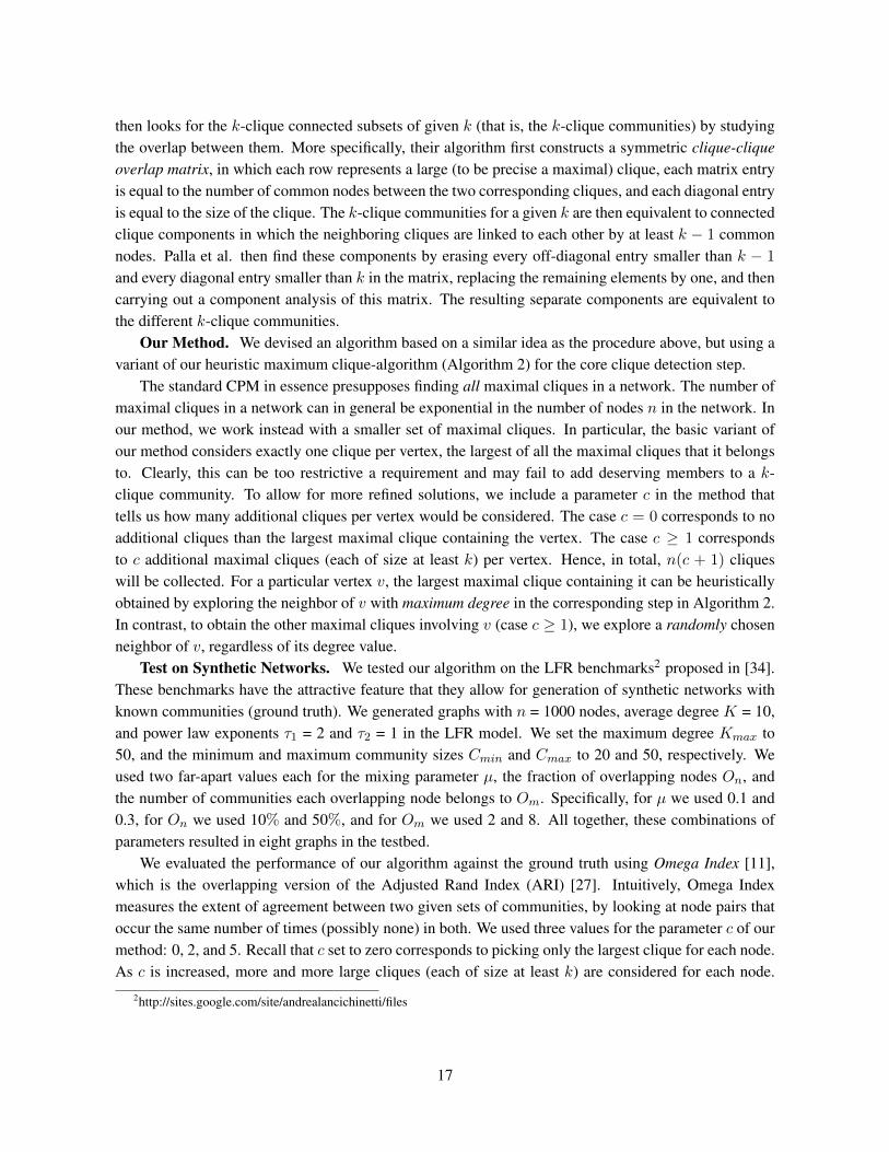
Table 5: Results of communities detected using our new method and CFinder on LFR benchmarks [34].All networks have n = 1000 nodes, and the parameters used to generate the netwroks are listed in thefirst three columns: µ is the mixing parameter, Om is the number of communities each overlapping nodeis assigned to On is the fraction of overlapping nodes. C(GT ) is the number of communities in the inputgraph (ground truth). C denotes the number of communities, S the number of shared nodes, and Ω theomega index.

CFinder Our Methodc = 0 c = 2 c = 5

µ Om On C(GT ) C S Ω C S Ω C S Ω C S Ω

0.1 2 10% 34 37 55 0.842 60 64 0.758 49 76 0.825 40 59 0.8400.1 2 50% 44 62 153 0.402 87 116 0.280 83 158 0.363 68 158 0.3950.1 8 10% 51 58 30 ∼0.0 76 46 ∼0.0 65 39 ∼0.0 61 35 ∼0.00.1 8 50% 130 74 68 0.030 74 56 0.020 79 66 0.028 79 72 0.0300.3 2 10% 35 50 53 0.612 69 67 0.461 64 73 0.577 55 60 0.6050.3 2 50% 44 60 95 0.193 92 93 0.109 85 102 0.152 77 106 0.1690.3 8 10% 48 64 35 0.304 79 59 0.239 74 55 0.293 69 46 0.3010.3 8 50% 142 57 43 0.019 58 46 0.013 61 49 0.017 59 45 0.018

Table 5 shows the experimental results we obtained. The first three columns of the Table list thevarious parameters used to generate each test network. The fourth column lists the number of groundtruth communities (C(GT )) in each network. The remaining columns in the table show performancein terms of the number of communities detected (C), total number of shared nodes (S) and the OmegaIndex (Ω) for CFinder and our method with different values for the parameter c. In our experiments, forCFinder as well as all variants of our algorithm, we found that the value of k = 4 gives the best OmegaIndex value relative to the ground truth. All results reported in Table 5 are therefore for k = 4.

In general we observe that there is a close correlation between our method and CFinder in terms ofall three of the quantities C, S and Ω. It can be seen that as we increase the value of c in our method,the Omega Index values get closer and closer to that of CFinder. For our algorithm run with c = 0, theOmega Index is about 75% of that of CFinder. When run with c = 2, it is about 92% and for c = 5, it isabout 99%. When we increased the value of c even further to 10, we observed that the Omega Index wasalmost identical to that obtained by CFinder. From this, one can see that we can get almost exactly thesame results as the CPM method using our algorithm which uses only a small set of maximal cliques, asopposed to all the maximal cliques in the graph.

Table 6 shows the time taken by CFinder and our method run with c = 0, 2 and 5. For our method,the table lists the total run time τ as well as the time τc spent on just the clique detection part and theratio τc/τ expressed in percents (τc%). The remaining time τ − τc is spent on building the clique-cliqueoverlap matrix, eliminating cliques, component analysis and generating the communities. As a sidenote, we point out that our immediate goal in the implementation of these later phases has been quick

3http://www.cfinder.org

18

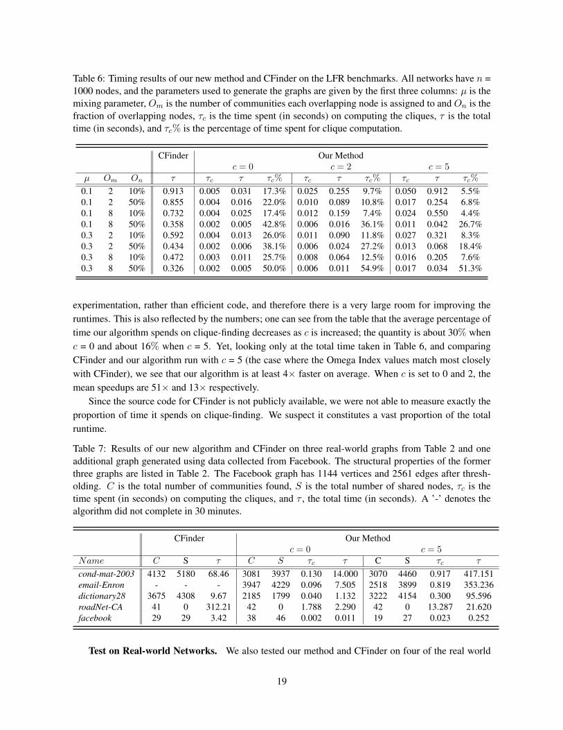
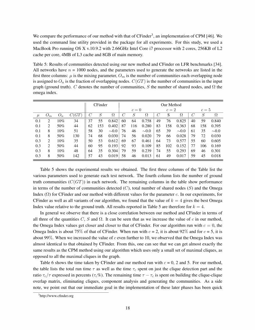
Table 6: Timing results of our new method and CFinder on the LFR benchmarks. All networks have n =1000 nodes, and the parameters used to generate the graphs are given by the first three columns: µ is themixing parameter, Om is the number of communities each overlapping node is assigned to and On is thefraction of overlapping nodes, τc is the time spent (in seconds) on computing the cliques, τ is the totaltime (in seconds), and τc% is the percentage of time spent for clique computation.

CFinder Our Methodc = 0 c = 2 c = 5

µ Om On τ τc τ τc% τc τ τc% τc τ τc%

0.1 2 10% 0.913 0.005 0.031 17.3% 0.025 0.255 9.7% 0.050 0.912 5.5%0.1 2 50% 0.855 0.004 0.016 22.0% 0.010 0.089 10.8% 0.017 0.254 6.8%0.1 8 10% 0.732 0.004 0.025 17.4% 0.012 0.159 7.4% 0.024 0.550 4.4%0.1 8 50% 0.358 0.002 0.005 42.8% 0.006 0.016 36.1% 0.011 0.042 26.7%0.3 2 10% 0.592 0.004 0.013 26.0% 0.011 0.090 11.8% 0.027 0.321 8.3%0.3 2 50% 0.434 0.002 0.006 38.1% 0.006 0.024 27.2% 0.013 0.068 18.4%0.3 8 10% 0.472 0.003 0.011 25.7% 0.008 0.064 12.5% 0.016 0.205 7.6%0.3 8 50% 0.326 0.002 0.005 50.0% 0.006 0.011 54.9% 0.017 0.034 51.3%

experimentation, rather than efficient code, and therefore there is a very large room for improving theruntimes. This is also reflected by the numbers; one can see from the table that the average percentage oftime our algorithm spends on clique-finding decreases as c is increased; the quantity is about 30% whenc = 0 and about 16% when c = 5. Yet, looking only at the total time taken in Table 6, and comparingCFinder and our algorithm run with c = 5 (the case where the Omega Index values match most closelywith CFinder), we see that our algorithm is at least 4× faster on average. When c is set to 0 and 2, themean speedups are 51× and 13× respectively.

Since the source code for CFinder is not publicly available, we were not able to measure exactly theproportion of time it spends on clique-finding. We suspect it constitutes a vast proportion of the totalruntime.

Table 7: Results of our new algorithm and CFinder on three real-world graphs from Table 2 and oneadditional graph generated using data collected from Facebook. The structural properties of the formerthree graphs are listed in Table 2. The Facebook graph has 1144 vertices and 2561 edges after thresh-olding. C is the total number of communities found, S is the total number of shared nodes, τc is thetime spent (in seconds) on computing the cliques, and τ , the total time (in seconds). A ’-’ denotes thealgorithm did not complete in 30 minutes.

CFinder Our Methodc = 0 c = 5

Name C S τ C S τc τ C S τc τ

cond-mat-2003 4132 5180 68.46 3081 3937 0.130 14.000 3070 4460 0.917 417.151email-Enron - - - 3947 4229 0.096 7.505 2518 3899 0.819 353.236dictionary28 3675 4308 9.67 2185 1799 0.040 1.132 3222 4154 0.300 95.596roadNet-CA 41 0 312.21 42 0 1.788 2.290 42 0 13.287 21.620facebook 29 29 3.42 38 46 0.002 0.011 19 27 0.023 0.252

Test on Real-world Networks. We also tested our method and CFinder on four of the real world

19

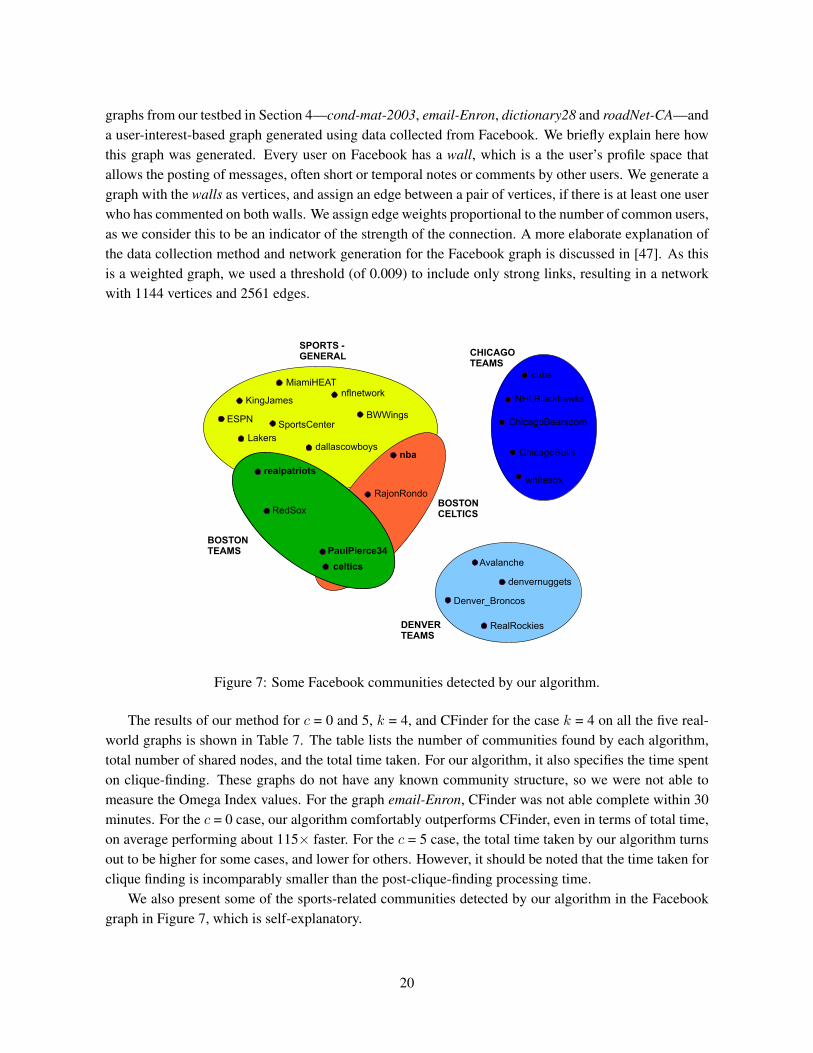
graphs from our testbed in Section 4—cond-mat-2003, email-Enron, dictionary28 and roadNet-CA—anda user-interest-based graph generated using data collected from Facebook. We briefly explain here howthis graph was generated. Every user on Facebook has a wall, which is a the user’s profile space thatallows the posting of messages, often short or temporal notes or comments by other users. We generate agraph with the walls as vertices, and assign an edge between a pair of vertices, if there is at least one userwho has commented on both walls. We assign edge weights proportional to the number of common users,as we consider this to be an indicator of the strength of the connection. A more elaborate explanation ofthe data collection method and network generation for the Facebook graph is discussed in [47]. As thisis a weighted graph, we used a threshold (of 0.009) to include only strong links, resulting in a networkwith 1144 vertices and 2561 edges.

ESPN

Lakers

realpatriots

dallascowboysnba

MiamiHEATnflnetwork

KingJames

BWWingsSportsCenter

PaulPierce34

celtics

RajonRondo

SPORTS - GENERAL

BOSTON CELTICS

BOSTON TEAMS

RedSox

Avalanche

Denver_Broncos

RealRockies

NHLBlackhawks

ChicagoBulls

ChicagoBearscom

cubs

whitesox

denvernuggets

CHICAGO TEAMS

DENVER TEAMS

Figure 7: Some Facebook communities detected by our algorithm.

The results of our method for c = 0 and 5, k = 4, and CFinder for the case k = 4 on all the five real-world graphs is shown in Table 7. The table lists the number of communities found by each algorithm,total number of shared nodes, and the total time taken. For our algorithm, it also specifies the time spenton clique-finding. These graphs do not have any known community structure, so we were not able tomeasure the Omega Index values. For the graph email-Enron, CFinder was not able complete within 30minutes. For the c = 0 case, our algorithm comfortably outperforms CFinder, even in terms of total time,on average performing about 115× faster. For the c = 5 case, the total time taken by our algorithm turnsout to be higher for some cases, and lower for others. However, it should be noted that the time taken forclique finding is incomparably smaller than the post-clique-finding processing time.

We also present some of the sports-related communities detected by our algorithm in the Facebookgraph in Figure 7, which is self-explanatory.

20

7 Conclusion

We presented a new exact and a new heuristic algorithm for the maximum clique problem. We performedextensive experiments on three broad categories of graphs comparing the performance of our algorithmsto the algorithms by Carraghan and Pardalos (CP) [9], Ostergard (cliquer) [45], Tomita et al. (MCQ,MCS) [54][55], Konc and Janezic (MCQD) [31], and Segundo et al. (BBMC) [53]. For DIMACSbenchmark graphs and certain dense synthetic graphs (rmat sd2), our new exact algorithm performscomparably with the CP algorithm, but slower than the others. For large sparse graphs, both syntheticand real-world, our new algorithm runs several orders of magnitude faster than the others. And its generalruntime is observed to grow nearly linearly with the size of the graphs. The heuristic, which runs ordersof magnitude faster than our exact algorithm and the others, delivers an optimal solution for 83% ofthe test cases, and when it is sub-optimal, its accuracy ranges between 0.83 and 0.99 for the graphs inour testbed. We also showed how the algorithms can be parallelized. Finally as a demonstration to theapplications of clique finding algorithms, we presented a novel and efficient alternative based on ouralgorithms to the Clique Percolation Method [46], to detect overlapping communities in networks.

Maximum clique detection is often avoided by practitioners from being used as a component in anetwork analysis algorithm on the grounds of its NP-hardness. The results shown here suggest that thisis not necessarily true, as maximum cliques can in fact be detected rather quickly for most real-worldnetworks that are characterized by sparsity and other structures well suited for branch-and-bound typealgorithms.

Acknowledgements

This work is supported in part by the following grants: NSF awards CCF-0833131, CNS-0830927, IIS-0905205, CCF-0938000, CCF-1029166, and OCI-1144061; DOE awards DE-FG02-08ER25848, de-sc0001283, de-sc0005309, de-sc0005340, and de-sc0007456; AFOSR award FA9550-12-1-0458. Thework of Assefaw Gebremedhin is supported in part by the NSF award CCF-1218916 and by the DOEaward de-sc0010205.

References

[1] D. Andrade, M. Resende, and R. Werneck, Fast local search for the maximum independent setproblem. Journal of Heuristics 18(4), pp. 525–547, 2012.

[2] J. G. Augustson and J. Minker, An analysis of some graph theoretical cluster techniques. Journalof the ACM 17(4), pp. 571–588, 1970.

[3] L. Babel and G. Tinhofer, A branch and bound algorithm for the maximum clique problem. Mathe-matical Methods of Operations Research 34(3), pp. 207–217, 1990.

[4] V. Batagelj and A. Mrvar, Pajek datasets, 2006. http://vlado.fmf.uni-lj.si/pub/networks/data/

[5] V. Boginski, S. Butenko, and P.M. Pardalos, Statistical analysis of financial networks. Computa-tional Statistics & Data Analysis 48(2), pp. 431–443, 2005.

21

[6] I. M. Bomze, M. Budinich, P. M. Pardalos, and M. Pelillo, The Maximum Clique Problem. Hand-book of Combinatorial Optimization, Kluwer Academic Publishers, pp. 1–74, 1999.

[7] R. E. Bonner, On some clustering techniques. IBM Journal of Research and Development 8(1), pp.22–32, 1964.

[8] A. E. Brouwer, J. B. Shearer, N. J. A. Sloane, and W. D. Smith, A new table of constant weightcodes. IEEE Transactions on Information Theory 36(6), pp. 1334–1380, 1990.

[9] R. Carraghan and P. Pardalos, An exact algorithm for the maximum clique problem. OperationsResearch Letters 9(6), pp. 375–382, 1990.

[10] D. Chakrabarti and C. Faloutsos, Graph mining: Laws, generators, and algorithms. ACM Comput-ing Surveys 38(1), 2006.

[11] L. M. Collins and C. W. Dent. Omega: A general formulation of the rand index of cluster recoverysuitable for non-disjoint solutions. Multivariate Behavioral Research 23(2), pp. 231–242, 1988.

[12] S. R. Corman, T. Kuhn, R. D. Mcphee, and K. J. Dooley. Studying complex discursive systems:Centering resonance analysis of communication. Human Communication Research 28(2), 157–206, 2002.

[13] T. A. Davis and Y. Hu, The university of florida sparse matrix collection. ACM Transactions onMathematical Software (TOMS) 38(1), pp. 1–25, 2011.

[14] P. Domingos and M. Richardson, Mining the network value of customers, in Proceedings of the 7thACM SIGKDD (KDD’01), ACM, New York, NY, USA, pp. 57–66, 2001.

[15] D. Eppstein and D. Strash. Listing all maximal cliques in large sparse real-world graphs, in Pro-ceedings of the 10th International Conference on Experimental Algorithms (SEA’11), P. M. Parda-los and S. Rebennack (Eds.), Springer-Verlag Berlin Heidelberg, pp. 364–375. 2011.

[16] M. Faloutsos, P. Faloutsos, and C. Faloutsos, On power-law relationships of the internet topology,in Proceedings of the Conference on Applications, Technologies, Architectures, and Protocols forComputer Communication, SIGCOMM ’99, ACM, New York, NY, USA, pp. 251–262, 1999.

[17] M. Ferronato, C. Janna, G. Gambolati, Mixed constraint preconditioning in computational contactmechanics. Computer Methods in Applied Mechanics and Engineering 197(45-48), pp. 3922–3931,2008.

[18] S. Fortunato, Community detection in graphs. Physics Reports 486(3), pp. 75–174, 2010.[19] M. R. Garey and D. S. Johnson, Computers and intractability: A guide to the theory of NP-

Completeness. W. H. Freeman & Co., New York, NY, USA, 1979.[20] S. Gregory. Fuzzy overlapping communities in networks. Journal of Statistical Mechanics: Theory

and Experiment 2011(2), 2011.[21] A. Grosso, M. Locatelli, and W. Pullan, Simple ingredients leading to very efficient heuristics for

the maximum clique problem. Journal of Heuristics 14(6), pp. 587–612, 2008.[22] G. Gutin, J. Gross, J. Yellen, Discrete Mathematics & Its Applications. Handbook of Graph Theory,

CRC Press, 2004.[23] B. H. Hall, A. B. Jaffe, and M. Trajtenberg. The NBER patent citation data file: Lessons, insights

and methodological tools. Technical Report, NBER Working Paper, 8498, 2001.[24] F. Havemann, M. Heinz, A. Struck, and J. Glaser. Identification of overlapping communities and

their hierarchy by locally calculating community-changing resolution levels. Journal of StatisticalMechanics: Theory and Experiment 1(23), 2011.

22

[25] R. Horaud and T. Skordas, Stereo correspondence through feature grouping and maximal cliques.IEEE Transactions on Pattern Analysis and Machine Intellence 11(11), pp. 1168–1180, 1989.

[26] D. Howe, Foldoc: Free on-line dictionary of computing. http://foldoc.org/.[27] L. Hubert and P. Arabie. Comparing partitions. Journal of Classification 2(1), pp. 193–218, 1985.[28] D. Johnson and M.A. Trick, Editors, Cliques, coloring and satisfiability: Second dimacs implemen-

tation challenge. DIMACS Series on Discrete Mathematics and Theoretical Computer Science 26,1996.

[29] Kdd cup, 2003. http://www.cs.cornell.edu/projects/kddcup/index.html.[30] G. R. Kiss, C. Armstrong, R. Milroy, and L. Piper. An associative thesaurus of English and its

computer analysis. The Computer and Literary Studies, Edinburgh University Press, 1973.[31] J. Konc and D. Janezic, An improved branch and bound algorithm for the maximum clique problem.

MATCH Communications in Mathematical Computer Chemistry 58, pp. 569–590, 2007.[32] R. Kumar, P. Raghavan, S. Rajagopalan, and A. Tomkins, Extracting Large-Scale Knowledge Bases

from the Web, in In Proceedings of the 25th International Conference on Very Large Data Bases(VLDB’99), M. P. Atkinson, M. E. Orlowska, P. Valduriez, S. B. Zdonik, and M. L. Brodie (Eds.),Morgan Kaufmann Publishers Inc., San Francisco, CA, USA, pp. 639–650,1999.

[33] A. Lancichinetti, S. Fortunato, and J. Kertesz. Detecting the overlapping and hierarchical commu-nity structure of complex networks. New Journal of Physics 11(3), p. 033015, 2009.

[34] A. Lancichinetti, S. Fortunato, and F. Radicchi. Benchmark graphs for testing community detectionalgorithms. Physical Review E 78(4), p. 046110, 2008.

[35] J. Leskovec, Stanford large network dataset collection. http://snap.stanford.edu/data/index.html.

[36] Google programming contest, 2002. http://www.google.com/

programming-contest/.[37] J. Leskovec, L. Adamic, and B. Adamic. The dynamics of viral marketing. ACM Transactions on

the Web 1(1), 2007.[38] J. Leskovec, D. Huttenlocher, and J. Kleinberg. Predicting positive and negative links in on-

line social networks, In Proceedings of the 19th International Conference on World Wide Web(WWW’10), pp. 641650, ACM, New York, NY, 2010.

[39] J. Leskovec, J. Kleinberg, and C. Faloutsos. Graph evolution: Densification and shrinking diame-ters. ACM Transactions on Knowledge Discovery from Data 1(1), 2007.

[40] J. Leskovec, J. Kleinberg, and C. Faloutsos, Graphs over time: Densification laws, shrinking di-ameters and possible explanations, in Proceedings of the eleventh ACM SIGKDD InternationalConference on Knowledge Discovery in Data Mining (KDD’05), ACM, New York, NY, USA, pp.177–187, 2005.

[41] L. Leydesdorff, On the normalization and visualization of author co-citation data: Salton’s cosineversus the jaccard index. Journal of the Association for Information Science and Technology 59(1),pp. 77–85, 2008.

[42] C. McCreesh and P. Prosser. Multi-threading a state-of-the-art maximum clique algorithm. Algo-rithms 6(4), pp. 618–635, 2013.

[43] M. E. J. Newman, Coauthorship networks and patterns of scientific collaboration, in Proceedingsof the National Academy of Sciences of the United States of America 101, pp. 5200–5205, 2004.

23

[44] S. Niskanen and P.R.J. Ostergard, Cliquer user’s guide, version 1.0, Technical Report T48, Com-munications Laboratory, Helsinki University of Technology, Espoo, Finland, 2003.

[45] P. R. J. Ostergard, A fast algorithm for the maximum clique problem. Discrete Applied Mathematics120(1-3), pp. 197–207, 2002.

[46] G. Palla, I. Derenyi, I. Farkas, and T. Vicsek. Uncovering the overlapping community structure ofcomplex networks in nature and society. Nature 435, pp. 814–818, 2005.

[47] D. Palsetia, M. M. Patwary, A. Agrawal, and A. Choudhary. Excavating social circles via userinterests. Social Network Analysis and Mining 4(1), pp. 1–12, 2014.

[48] P. M. Pardalos and J. Xue, The maximum clique problem. Journal of Global Optimization 4, pp.301–328, 1994.

[49] M. Pavan and M. Pelillo, A new graph-theoretic approach to clustering and segmentation, in Pro-ceedings of the IEEE Conference on Computer Vision and Pattern Recognition (CVPR’03), IEEEComputer Society, Washington, DC, USA, pp. 145–152, 2003.

[50] P. Prosser. Exact algorithms for maximum clique: A computational study. Algorithms, 5(4), pp.545–587, 2012.

[51] M. Richardson, R. Agrawal, and P. Domingos. Trust management for the semantic web, In Pro-ceedings of the Second International Semantic Web Conference (ISWC), Springer-Verlag BerlinHeidelberg, pp. 351–368, 2003.

[52] S. Sadi, S. Oguducu, and A.S. Uyar, An efficient community detection method using parallel clique-finding ants, in Proceedings of the IEEE Congress on Evolutionary Computation, pp. 1–7, 2010.

[53] P. San Segundo, D. Rodrıguez-Losada, and A. Jimenez, An exact bit-parallel algorithm for themaximum clique problem. Computers & Operations Research 38(2), pp. 571–581, 2011.

[54] E. Tomita and T. Seki, An efficient branch-and-bound algorithm for finding a maximum clique, inProceedings of the 4th International Conference on Discrete Mathematics and Theoretical Com-puter Science, Springer-Verlag Berlin Heidelberg, pp. 278–289, 2003.

[55] E. Tomita, Y. Sutani, T. Higashi, S. Takahashi, and M. Wakatsuki, A simple and faster branch-and-bound algorithm for finding a maximum clique, in Proceedings of the 4th International Workshopon Algorithms and Computation (WALCOM), M. Rahman and S. Fujita (Eds.), Springer BerlinHeidelberg, pp. 191–203, 2010.

[56] T. Matsunaga, C. Yonemori, E. Tomita, and M. Muramatsu, Clique-based data mining for relatedgenes in a biomedical database. BMC Bioinformatics 10, p. 205, 2010.

[57] J. Turner, Almost all k-colorable graphs are easy to color, Journal of Algorithms 9, pp. 63–82,1988.

[58] B. van Rietbergen, H. Weinans, R. Huiskes, and A. Odgaard, A new method to determine trabec-ular bone elastic properties and loading using micromechanical finite-element models. Journal ofBiomechanics 28(1), pp. 69 – 81, 1995.

[59] L. Wang, L. Zhou, J. Lu, and J. Yip, An order-clique-based approach for mining maximal co-locations. Information Sciences 179(19), pp. 3370–3382, 2009.

[60] J. Xie, S. Kelley, and B. K. Szymanski. Overlapping community detection in networks: The state-of-the-art and comparative study. ACM Computing Surveys 45(4), pp. 43:1–43:35, 2013.

24

Appendix

Table 8: Comparison of runtimes of our new exact maximum clique finding algorithm (τA1) and themaximal clique enumeration algorithm by Eppstein & Strash [15] (τES) for the Pajek and Stanford datasets in our testbed. The runtimes under column τES are directly quoted from [15]. The column ∆ denotesthe maximum degree, and ω the maximum clique size of the graph.

G |V | |E| ∆ ω τA1 τES [15]foldoc 13,356 91,470 728 9 0.05 0.13eatRS 23,219 304,938 1090 9 1.81 1.03hep-th 27,240 341,923 2411 23 4.48 1.70patents 240,547 560,943 212 6 0.13 1.65days-all 13,308 148,035 2265 28 75.37 5.18

roadNet-TX 1,393,383 1,921,660 12 4 0.26 4.00amazon0601 403,394 2,247,318 2752 11 0.20 6.03email-EuAll 265,214 364,481 7636 16 0.92 1.33web-Google 916,428 4,322,051 6332 44 0.35 9.70soc-wiki-Vote 8,297 100,762 1065 17 4.31 1.14soc-slashdot0902 82,168 504,230 2252 27 25.54 2.58cit-Patents 3,774,768 16,518,947 793 11 19.99 58.64soc-Epinions1 75,888 405,740 3044 23 15.01 4.78soc-wiki-Talk 2,394,385 4,659,565 100029 26 6885.13 216.00web-berkstan 685,230 6,649,470 84230 201 44.70 20.87

25

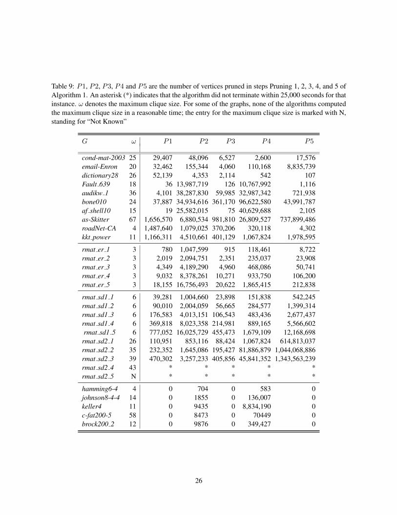
Table 9: P1, P2, P3, P4 and P5 are the number of vertices pruned in steps Pruning 1, 2, 3, 4, and 5 ofAlgorithm 1. An asterisk (*) indicates that the algorithm did not terminate within 25,000 seconds for thatinstance. ω denotes the maximum clique size. For some of the graphs, none of the algorithms computedthe maximum clique size in a reasonable time; the entry for the maximum clique size is marked with N,standing for “Not Known”

G ω P1 P2 P3 P4 P5

cond-mat-2003 25 29,407 48,096 6,527 2,600 17,576email-Enron 20 32,462 155,344 4,060 110,168 8,835,739dictionary28 26 52,139 4,353 2,114 542 107Fault 639 18 36 13,987,719 126 10,767,992 1,116audikw 1 36 4,101 38,287,830 59,985 32,987,342 721,938bone010 24 37,887 34,934,616 361,170 96,622,580 43,991,787af shell10 15 19 25,582,015 75 40,629,688 2,105as-Skitter 67 1,656,570 6,880,534 981,810 26,809,527 737,899,486roadNet-CA 4 1,487,640 1,079,025 370,206 320,118 4,302kkt power 11 1,166,311 4,510,661 401,129 1,067,824 1,978,595

rmat er 1 3 780 1,047,599 915 118,461 8,722rmat er 2 3 2,019 2,094,751 2,351 235,037 23,908rmat er 3 3 4,349 4,189,290 4,960 468,086 50,741rmat er 4 3 9,032 8,378,261 10,271 933,750 106,200rmat er 5 3 18,155 16,756,493 20,622 1,865,415 212,838

rmat sd1 1 6 39,281 1,004,660 23,898 151,838 542,245rmat sd1 2 6 90,010 2,004,059 56,665 284,577 1,399,314rmat sd1 3 6 176,583 4,013,151 106,543 483,436 2,677,437rmat sd1 4 6 369,818 8,023,358 214,981 889,165 5,566,602rmat sd1 5 6 777,052 16,025,729 455,473 1,679,109 12,168,698

rmat sd2 1 26 110,951 853,116 88,424 1,067,824 614,813,037rmat sd2 2 35 232,352 1,645,086 195,427 81,886,879 1,044,068,886rmat sd2 3 39 470,302 3,257,233 405,856 45,841,352 1,343,563,239rmat sd2 4 43 * * * * *rmat sd2 5 N * * * * *

hamming6-4 4 0 704 0 583 0johnson8-4-4 14 0 1855 0 136,007 0keller4 11 0 9435 0 8,834,190 0c-fat200-5 58 0 8473 0 70449 0brock200 2 12 0 9876 0 349,427 0

26

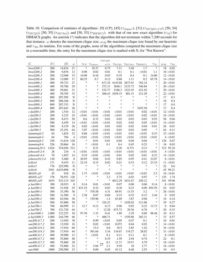
Table 10: Comparison of runtimes of algorithms: [9] (CP), [45] (τcliquer), [31] (τMCQD+CS), [50, 54](τMCQ1), [50, 55] (τMCSa1), and [50, 53] (τBBMC1). with that of our new exact algorithm (τA1) forDIMACS graphs. An asterisk (*) indicates that the algorithm did not terminate within 7,200 seconds forthat instance. ω denotes the maximum clique size, ωA2 the maximum clique size found by our heuristicand τA2, its runtime. For some of the graphs, none of the algorithms computed the maximum clique sizein a reasonable time; the entry for the maximum clique size is marked with N, for “Not Known”.

τMCQD

G |V | |E| ω τCP τcliquer +CS τMCQ1 τMCSa1 τBBMC1 τA1 ωA2 τA2

brock200 1 200 14,834 21 * 10.37 0.75 7.11 5.48 1.7 * 18 0.02brock200 2 200 9,876 12 0.98 0.02 0.01 0.1 0.1 <0.01 1.1 10 <0.01brock200 3 200 12,048 15 14.09 0.16 0.03 0.35 0.4 0.1 14.86 12 <0.01brock200 4 200 13,089 17 60.25 0.7 0.12 0.88 1.11 0.2 65.78 14 <0.01brock400 1 400 59,723 27 * * 671.24 4145.68 2873.91 762.14 * 20 <0.01brock400 2 400 59,786 29 * * 272.31 2848.1 2123.73 546.84 * 20 <0.01brock400 3 400 59,681 31 * * 532.77 2186.3 1523.55 431.92 * 20 <0.01brock400 4 400 59,765 33 * * 266.43 1038.33 881.31 211.29 * 22 <0.01brock800 1 800 207,505 N * * * * * * * 17 0.3brock800 2 800 208,166 N * * * * * * * 18 0.4brock800 3 800 207,333 N * * * * * * * 17 0.4brock800 4 800 207,643 26 * * * * * 3455.58 * 17 0.4c-fat200-1 200 1,534 12 <0.01 <0.01 <0.01 <0.01 <0.01 0.02 <0.01 12 <0.01c-fat200-2 200 3,235 24 <0.01 <0.01 <0.01 <0.01 <0.01 0.02 <0.01 24 <0.01c-fat200-5 200 8,473 58 0.6 0.33 0.01 0.03 0.03 0.03 0.93 58 0.04c-fat500-1 500 4,459 14 <0.01 <0.01 <0.01 0.02 0.02 0.05 <0.01 14 <0.01c-fat500-2 500 9,139 26 0.02 <0.01 0.01 0.02 0.02 0.04 0.01 26 0.01c-fat500-5 500 23,191 64 3.07 <0.01 <0.01 0.03 0.03 0.05 * 64 0.11hamming6-2 64 1,824 32 0.68 <0.01 <0.01 <0.01 0.01 <0.01 0.33 32 <0.01hamming6-4 64 704 4 <0.01 <0.01 <0.01 <0.01 <0.01 <0.01 <0.01 4 <0.01hamming8-2 256 31,616 128 * 0.01 0.01 0.04 0.04 0.04 * 128 0.67hamming8-4 256 20,864 16 * <0.01 0.1 0.4 0.45 0.23 * 16 0.03hamming10-2 1,024 518,656 512 * 0.31 - 0.36 0.371 0.13 * 512 95.24johnson8-2-4 28 210 4 <0.01 <0.01 <0.01 <0.01 <0.01 <0.01 <0.01 4 <0.01johnson8-4-4 70 1,855 14 0.19 <0.01 <0.01 0.01 0.02 0.01 0.23 14 <0.01johnson16-2-4 120 5,460 8 20.95 0.04 0.42 0.85 0.95 0.41 22.07 8 <0.01keller4 171 9,435 11 22.19 0.15 0.02 0.21 0.33 0.12 23.35 11 <0.01keller5 776 225,990 N * * * * * * * 22 0.6keller6 3361 4,619,898 N * * * * * * * 45 99.21MANN a9 45 918 16 1.73 <0.01 <0.01 <0.01 <0.01 <0.01 2.5 16 <0.01MANN a27 378 70,551 126 * * 3.3 5.75 6.03 0.97 * 125 1.74MANN a45 1035 533,115 345 * * * 4612.29 3431.67 250.12 * 341 59.96p hat300-1 300 10,933 8 0.14 0.01 <0.01 0.07 0.08 0.06 0.14 8 <0.01p hat300-2 300 21,928 25 831.52 0.32 0.03 0.38 0.23 0.09 854.59 24 0.03p hat300-3 300 33,390 36 * 578.58 4.31 69.91 13.53 3.2 * 26 <0.01p hat500-1 500 31,569 9 2.38 0.07 0.04 0.33 0.35 0.12 2.44 9 0.02p hat500-2 500 62,946 36 * 159.96 1.2 63.89 3.87 0.96 * 34 0.14p hat500-3 500 93,800 50 * * 324.23 * 1428.02 311.06 * 39 0.27p hat700-1 700 60,999 11 12.7 0.12 0.13 0.96 0.92 0.23 12.73 9 0.04p hat700-2 700 121,728 44 * * 12.28 675.72 29.36 6.76 * 26 0.15p hat1000-1 1,000 122,253 10 97.39 1.33 0.41 1.89 2.29 0.69 98.48 10 0.11p hat1000-2 1,000 244,799 46 * * 406.71 * 1359.88 382.31 * 33 0.57san200 0.7 1 200 13,930 30 * 0.99 <0.01 0.05 0.47 0.1 * 16 0.01san200 0.7 2 200 13,930 18 * 0.02 <0.01 0.072 0.04 0.03 * 14 <0.01san200 0.9 2 200 17,910 60 * 13.4 0.8 18.5 5.85 1.42 * 34 <0.01san200 0.9 3 200 17,910 44 * 561.64 3.16 134.67 119.27 28.02 * 31 <0.01san400 0.5 1 400 39,900 13 * <0.01 0.1 0.11 0.11 0.1 * 8 <0.01san400 0.7 1 400 55,860 40 * * 0.35 1.59 2.94 0.74 * 22 0.1san400 0.7 2 400 55,860 30 * * 0.1 12.71 19.51 4.79 * 18 <0.01san400 0.7 3 400 55,860 22 * 5.04 2.1 9.59 10 2.77 * 16 <0.01san1000 1000 250,500 15 * 0.09 0.45 43.12 8.48 2.55 * 10 0.5

27